Innovative Approach for Urban Stream Restoration

Undergraduate Thesis CHBE 494

Kosta Sainis

Thesis Advisor Dr. Royann Petrell

Submitted: April 7, 2006

University of British Columbia Chemical and Biological Engineering

i

EXECUTIVE SUMMARY

The novelty of this study is the design of a stream which is able to manage stormwater as

well as provide fish habitat. A design methodology which can be used to develop a pond

and stream system suitable for the University of British Columbia South Campus

Neighbourhood and fish habitat was developed.

Federal and provincial guidelines recommend that post development runoff volumes

roughly equal pre-development runoff volume, and that the total runoff volume is limited

to 10% or less of the total rainfall volume. With the addition of the pond and stream

system, post development runoff volumes differed from pre development runoff volumes

by an average of 15%. Although the post development runoff volumes did not equal the

predevelopment runoff volumes, the 6% decrease in runoff volume is a significant step

towards achieving post development runoff volumes, which roughly equal

predevelopment runoff volumes. The pond and stream system was unable to limit the

total runoff volume to 10% or less of the total rainfall volume. The pond and stream

system was only able to limit the total runoff volume to approximately 78% of the total

rainfall volume. This guideline may have been difficult to achieve since the pond and

stream system is only taking runoff from a small area of rooftops in comparison to the

large area, which makes up the South Campus Neighbourhood.

The implication of this study is that an urban stream, which is able to manage stormwater

as well as conform to fish habitat criteria, will flow through the University of British

Columbia campus. This will restore the fish-bearing stream, which once flowed through

campus. The vision is that fish will one day utilize the stream as habitat and spawning

areas. Implementation of such a stream and pond system will also help the University of

British Columbia to strive towards meeting federal and provincial stormwater

management guidelines. On a larger scale, the research promotes sustainability through

fish habitat conservation and efficient use of water resources.

ii

TABLE OF CONTENTS EXECUTIVE SUMMARY……………………………………………………………...i LIST OF FIGURES…………………………………………………………………….iv LIST OF TABLES……………………………………………………………………...vi 1.0 INTRODUCTION………………………………………………………………...…1 2.0 THESIS OBJECTIVES…………………………………………………………...…5 3.0 BACKGROUND AND DESIGN INFORMATION

3.1 Cutthroat Trout Life History Strategy and Habitat Requirements…………....7

3.2 Riffle Pool Streams…………………………………………………………...9

3.3 Stream Design Hydraulic Equations………………………………………...16

3.4 Major Urban Stream Issues……………………………………………….…28

3.5 Design of Piping Distribution System…………………………………….…35

4.0 DESIGN METHOLOGY AND SAMPLE SYSTEMS……………………….….37

PHASE 1: SITE ANALYSIS AND CONCEPTUAL MODEL DEVELOPMENT….....39

Phase 1.1 Site Description…………………………………………………….....39

Phase 1.2 Stream and Pond Placement Considerations…………………….…...40

Phase 1.3 Chosen Pond and Stream Placement………………………………....42

Phase 1.4 Location and Placement of riffle pool and cascade pool sequences....44

PHASE 2 CONCEPTUAL MODEL DEVELOPMENT…………………………….…47

PHASE 3 POND DESIGN AND DIMENSIONING……………………………….….53

PHASE 4 STREAM DESIGN AND DIMENSIONING…………………………….…59

PHASE 5 PIPING SYSTEM DESIGN………………………………………………...69

iii

5.0 RESULTS AND DISCUSSION…………………………………………………....72

6.0 CONCLUSION AND RECOMMENDATIONS…………………………….…....77

7.0 RESEARCH IMPLICATIONS…………………………………………………....79

ACKNOWLEDGEMENTS……………………………………………………………80

REFERENCES………………………………………………………………………….81

APPENDICES…………………………………………………………………………..84

APPENDIX A: TOPOGRAPHY MAP OF SOUTH CAMPUS………………...85 APPENDIX B: AERIAL PHOTOGRAPH OF SOUTH CAMPUS……………86 APPENDIX C: SOUTH CAMPUS LAND USE PLAN………………………...87 APPENDIX D: RATIONAL FORMULA RUNOFF COEFFICIENT, C TBL…88 APPENDIX E: PONDS, STREAM, AND CULVERT PLACMENT…………..89 APPENDIX F: SOUTH CAMPUS SUBDIVISION PLAN……………………..90 APPENDIX G: SAMPLE BOREHOLE RESULT……………………………...92 APPENDIX H: SAMPLE POND DIMENSION CALCULATIONS…………...93 APPENDIX I: UBC RAINFALL IDF CURVES……………………………......96 APPENDIX J: TYPICAL VEGETATION FOUND NEAR PONDS…………...97 APPENDIX K: RANDOMIZATION OF CASSCADE POOL & RIFFLE POOLS …………………………………………………………………………………...99 APPENDIX L: RANDOMIZATION OF DEGREE OF MEANDERING …………………………………………………………………………………..100 APPENDIX M: TOPOGRAPHY MAP OF SOUTH CAMPUS AREA……….101 APPENDIX N: SLOPE CALCULATIONS……………………………………102 APPENDIX O: UNDERCUT STREAM BANK………………………………102 APPENDIX P: WIDTH OF STREAM WITH ADDITIONAL FREEBOARD..103

iv

APPENDIX Q: DEPTH TO WIDTH RATIO CALCULATION EXAMPLE…103 APPENDIX R: DETERMINATION OF MANNING’S COEFFICIENT USING METHOD OUTLINED BY Arcement and Schneider 2005…………………...104 APPENDIX S: STREAM FLOWRATE VERSUS DISTANCE DOWNSTREAM ………………………………………………………………………………….108 APPENDIX T: STREAM DIMENSIONING DATA………………………….109 APPENDIX U: PIPE DISCHARGING INTO POND CROSS SECTION…….114 APPENDIX V: GUIDLINE CONFORMATION CALCULATIONS…………115 APPENDIX W: POND ROOFTOP DATA AND CALCULATIONS………...120 APPENDIX X: TIME IT TAKES FOR POND FILLING……………………..121

v

LIST OF FIGURES Figure 1 Aerial view of the proposed site for the University of British Columbia South Campus Neighbourhood………………………………………………………………….3 Figure 2 Proposed South Campus Neighbourhood Plan………………………………...4 Figure 3 Adult male and female cutthroat trout (Salmo clarki)…………………………7 Figure 4 The typical lifecycle of an anadromous cutthroat trout (Salmo clarki) and other salmonid species………………………………………………………………………....8 Figure 5 A typical stream with riffle pool sequence morphology………………………10 Figure 6 Cross sectional view of a stream………………………………………………13 Figure 7. A straight channeled stream typically seen in urban areas and a meandering, sinuous stream typically seen in natural environments………………………………….15 Figure 8 Routes in which water flow enters a stream…………………………………..18 Figure 9 Critical velocity with respect to stream bed material (sediment) diameter……23 Figure 10 Critical shear stresses according to shields…………………………………...25 Figure 11 Critical shear stress on banks…………………………………………………27 Figure 12 Area susceptible to erosion…………………………………………………..29 Figure 13 A natural riffle pool morphology stream lined with riparian vegetation…….32 Figure 14 The initial application of a geotextile along a stream bank…………………..33 Figure 15 The application of rip-rap along a stream bank to help prevent erosion……...34 Figure 16 Simplified concept behind a piping distribution system……………………...36 Figure 17 Recommended pond and stream placement…………………………………..42 Figure 18 South Campus Land Use Plan and recommended stream and pond locations..43 Figure 19 Recommended location of cascade pool and riffle pool sequences…………..45 Figure 20 Conceptual ponds and stream model…………………………………………47

vi

Figure 21 Pond Dimensions……………………………………………………………..55 Figure 22 Pond cross section…………………………………………………………….56 Figure 23 Emergency Spillway………………………………………………………….57 Figure 24 Cross sectional view of stream……………………………………………….62 Figure 25 Sample tabulation of stream at Section A……………………………………65 Figure 26 Critical velocity with respect to streambed material diameter……………….67

vii

LIST OF TABLES Table 1 Maximum swim speeds and jump height of adult and juvenile cutthroat trout (Salmo clarki)…………………………………………………………………………….9 Table 2 Typical channel and aquatic characteristics associated with the major morphological types: Step-pool, cascade-pool and riffle pool, and riffle pools with sand beds……………………………………………………………………………………...11 Table 3 Various stream cross sections and shapes………………………………………21

Table 4 Manning’s Roughness coefficients……………………………………………..64

1

1.0 INTRODUCTION Several natural streams in British Columbia have vanished or have been severely altered

(DFO 2005). Urbanization is one of the primary factors contributing to this decline

(Hunter 1991). The demand for urban development increases with human population

growth (Huth 1978). Unfortunately fish populations and stream habitat has diminished as

a result (DFO 2005). As well, water table levels have dropped forcing issues with

summer time irrigation and increased stormwater management costs in some areas

(Finkenbine 1998). Now is the time to incorporate streams with development plans to

mitigate losses, reduce costs, and help restore valuable fisheries resources for future

generations.

Interestingly, a stream suitable for fish has fewer issues related to water table levels

(Moyle and Chech 2004). A stream properly designed to receive stormwater directly and

indirectly, may lower stormwater management costs (MWLAP 2004). To improve fish

habitat in an existing stream, existing stream rehabilitation techniques can be used for

planning and implementation (Johnston and Slaney 1996). Restoration of an extinct

stream however, requires alternative techniques since water supply is no longer available

(Johnston and Slaney 1996). Urban stream restoration is an increasingly popular method

of reintroducing stream habitat (Hunter 1991). Although many methods of urban stream

restoration have been developed, few have been designed to suit fish habitat or collect

clean runoff as a means to sustain stream flow.

2

At the University of British Columbia, there is now the unique opportunity to restore a

stream that once flowed through it (Figure 1). This stream is part of the South Campus

neighbourhood, which is planned to be developed into a residential community in early

2006 (UBC 2004) (Figure 2). The South Campus neighbourhood makes up 22 ha of land

and lies in the Northeast Sub-area (Alpin and Martin 2005) (Figure 1 and 2). This area is

bounded by 16th Avenue to the north, Pacific Spirit Regional Park to the east, and Future

Reserve and Bio Sciences land to the south and the west (Alpin and Martin 2005) (Figure

1 and 2). Approximately 3.4 ha of the land have been allocated to useable neighbourhood

space (Alpin and Martin 2005).

High amounts of runoff volume are associated with the impermeable surfaces of urban

areas (MWLAP 2004). Current stormwater runoff guidelines for new areas of

development recommend that post development runoff volumes roughly equal pre-

development runoff volumes (MWLAP 2004). In addition, the British Columbia Ministry

of Environment states that an appropriate performance target for managing runoff volume

is to limit the total runoff volume to 10% (or less) of the total rainfall volume (BC

Ministry Environment 2002). Common best management practices which help to achieve

these goals include: ponds, stream restoration, and infiltration basins (MWLAP 2004).

Simon Fraser University is currently the leading university in British Columbia which

takes into consideration these guidelines and practices. These guidelines and practices

have been incorporated in their official community plan for new development since 1996

(SFU 2006). It is time that the University of British Columbia strive to meet these

guidelines; innovation would be expected of a university setting.

3

The innovative approach that is the focus of this thesis is to examine whether a

combination of common stormwater practices (i.e. ponds) and uncommon practices

(designing streams suited to fish habitat) can meet the stormwater guidelines.

Figure 1. Aerial view of the proposed site for the University of British Columbia South Campus Neighbourhood. The South Campus Neighbourhood lies within the broken black bordered line. The area within the yellow bordered line is the Northeast Sub-area of the University of British Columbia. The red line is the possible location of the fish bearing stream which once passed through this area. (Alpin and Martin 2005)

4

Figure 2. Proposed South Campus Neighbourhood Plan. Specific development on this site is not finalized.(Alpin and Martin 2005)

5

2.0 THESIS OBJECTIVES The overall objective is to develop a design methodology that can be used to design a

pond and stream system suitable for South Campus and fish habitat. If the stormwater

system is designed to meet recommended federal and provincial guidelines then the

following guidelines must be met:

That post development runoff volumes roughly equal pre-development runoff

volumes (MWLAP 2004).

The total runoff volume will be limited to 10% (or less) of the total rainfall

volume (BC Ministry of Environment 2002).

Based on the developed design methodology, the degree in which the above guidelines

can be met will be determined.

Sub-objectives include:

Development of a stream model supported by rooftop runoff through the

application fluid mechanics and consideration of fish habitat criteria.

Design the stream taking into consideration major urban stream issues such as

overflow, erosion, and periods of high and low flow.

Determine how to manage variable rooftop runoff flow of good water quality

without compromising critical stream velocities or jeopardizing fish habitat

6

criteria. This includes investigating the possible use of ponds to help manage

variable rooftop runoff flow.

Design of a piping distribution system for the new residential complex that will

receive rooftop runoff and effectively contribute to stream flow.

The stream will be restricted to the following constraints:

• Stream width will be no more than 2-3 m wide to accommodate space issues.

• The stream morphology will be dictated by the type most closely associated with

the land slope and flow conditions.

• The target fish species is cutthroat trout (Salmo clarki) because they are

associated with the land, slope, and flow conditions present of the system. In

addition, cutthroat trout utilize similar habitat to other salmonids such as coho

(Oncorhynchus kisutch) and chum (Oncorhynchus keta). Thus designing the

stream to suit cutthroat trout will ensure the stream meets habitat criteria of

several salmonid species.

• The runoff used to develop this methology will only come from rooftops because

this runoff unlike runoff from roads and parking areas is considered to be of

suitable quality for fish (MWLAP 2004).

7

3.0 BACKGROUND AND DESIGN INFORMATION

A literature review was conducted to attain the background information needed to

successfully design a stream similar to the one that once flowed through the South

Campus neighbourhood. To design a stream for the target fish species, knowing the life

history strategy and habitat is important (Hunter 1991). Thus, this section begins with

information on the life history strategy and habitat requirements of cutthroat trout.

Discussion then focuses on riffle pool and cascade pool streams which cutthroat trout

often reside in. Next commonly used hydraulic equations for stream design are reviewed,

followed by the major issues associated with urban streams. Finally basic design of a

piping distribution system which collects rooftop runoff and supplies flow to the stream

is investigated.

3.1 Cutthroat Trout Life History Strategy and Habitat Requirements Cutthroat trout (Salmo clarki) belong to the family Salmoninae which includes all salmon

and trout species (Moyle and Cech 2004). Cutthroat trout can be readily identified by

their blunt head, small black spots on their head and body which extends below the lateral

line, red to yellow streaks on the underside the jaw, faint to no red on the sides when

spawning, weights between 0.3 and 0.5 kg, and an average length of 45 cm (Moyle and

Cech 2004) (Figure 3).

Figure 3. Adult male and female cutthroat trout (Salmo clarki)

8

Cutthroat trout have anadromous and non-anadromous forms (DFO 2005). Anadromous

forms are born in freshwater systems, migrate to oceans to feed and grow, and later return

to freshwater systems to spawn (Moyle and Cech 2004). Figure 4 illustrates the typical

lifecycle of an anadromous salmonid.

Figure 4. The typical lifecycle of an anadromous cutthroat trout (Salmo clarki) and other salmonid species. (USDA 2005)

Non-anadromous forms spend their entire lifecycle in freshwater systems (Moyle and

Cech 2004). Cutthroat trout spawn between the months of February and May at the age of

three or four (DFO 2005). This is advantageous since February through May are months

of high rainfall at the University of British Columbia (Finkenbine 1998). This ensures

sufficient flow will be present in streams for cutthroat trout to spawn.

9

Stream temperature should not exceed 24oC for optimal reproduction and growth of

cutthroat trout (Moyle and Chech 2004). Cutthroat trout require a minimum stream depth

of 0.06 m, velocity between 0.11 to 0.72 m/s, substrate size of 6-102 mm, and a mean

redd area of 0.09-0.0 m2 for optimal spawning conditions (Hogan and Ward 1997). The

maximum swim speed and jumping height of cutthroat trout vary depending on its

current life stage (Hogan and Ward 1997). Table 1, summarizes the maximum sustained,

prolonged, and burst swimming speeds, as well as the maximum jumping height for

cutthroat trout at various stages in its lifecycle.

Table 1. Maximum swim speeds and jump height of adult and juvenile cutthroat trout (Salmo clarki). (Dane 1978)

Species Lifestage Maximum Swim Seed (m/s) Maximum Cutthroat Sustained Prolonged Burst Jump Height (m) adults 0.9 1.8 4.3 1.5 juveniles (125 mm) 0.4 0.7 1.1 0.6 juveniles (50 mm) 0.1 0.3 0.4 0.3

When designing a stream, it is important that these velocities and jumping heights are

taken into consideration to ensure fish are able to readily travel through the stream

(Hogan and Ward 1997). Cutthroat trout are often found in streams with riffle pool and

cascade pool morphology (Hogan and Ward 1997). These streams are suited to

accommodate cutthroat trout at the various stages of its lifecycle (Hogan and Ward 1997).

Riffle pool and cascade pool streams are discussed in the following section.

3.2 Riffle Pool and Cascade Pool Streams Riffle pool or cascade pool morphology streams are an ideal choice for an urban stream

taking fish habitat criteria into consideration. This is because they are relatively small in

10

size, making them ideal when space is limited (Hogan and Ward 1997). In addition, they

suit a variety of fish species (Hogan and Ward 1997). Riffles and cascades are shallow

areas of stream which provide aeration and increased current velocity (Hunter 1991)

(Figure 5). Pools are deeper areas with slower current velocity and are often used by fish

as refuge (Hunter 1991) (Figure 5).

Figure 5. A typical stream with riffle pool sequence morphology. Trout particularly like riffle and cascade pool sequences because its morphology suits

various stages of their life cycle (Hunter 1991). The reduced velocities in pools provide

an ideal refuge area for juvenile trout, while riffles or cascades continually carry food to

them (Hunter 1991). Deeper pools also provide refuge from predators, cooler

temperatures, and are essential to the over winter survival of trout (Moyle and Cech

2004).

11

Riffle pool and cascade pool morphologies are one of three major stream morphology

types (Hogan and Ward 1997). These include step-pools, cascade and riffle pools, and

riffle pools with sand beds (Hogan and Ward 1997). Channel and aquatic characteristics

of each stream morphology type is outlined in Table 2.

Table 2. Typical channel and aquatic characteristics associated with the major morphological types: Step-pool, cascade-pool and riffle pool, and riffle pools with sand beds. (Hogan and Ward 1997)

12

Key stream parameters to consider when designing a stream include bankfull width,

bankfull depth, dominant sediment size, and channel gradient (Hogan and Ward 1997).

Bankfull width is used as the base unit when stream dimensions are being determined

(Newbury et al. 1997). It is defined as the distance between the edges of a stream where

vegetation begins to grow (Newbury et al. 1997) (Figure 6). Bankfull width is used to

determine the spacing between cascades/riffles and pools in a cascade pool and riffle pool

sequenced stream (Newbury et al. 1997). Optimal pool to cascade/riffle spacing is

typically 6 to 8 times the bankfull width (Newbury et al. 1997). Bankfull depth is the

water surface elevation needed to fill the channel to the point in which water does not

spill into the flood plain (Newbury et al. 1997) (Figure 6). Bankfull depth is an important

parameter used to determine how much flow a stream can effectively handle (Newbury et

al. 1997). Dominant stream bed material size (or sediment size) is important since certain

sizes of stream bed materials are ideal for salmon spawning (Moyle and Cech 2004). The

ideal stream bed material for cutthroat trout is gravel with a diameter ranging from 6-

102mm (Hogan and Ward 1997). Stream bed material smaller than this size, may be

abrasive to fish eggs and damaging to gills (Moyle and Cech 2004). Designing a stream

to maintain a particular sediment size, while discharging smaller sediment sizes, is

discussed in the next section. Channel gradient is important since it plays a significant

role in stream velocity and discharge rate (Johnston and Slaney 1996). When designing

the stream a channel gradient of less than approximately 4% will be used to maintain

cascade pool or riffle pool stream morphology. A gradient of less than 4% is typical of

cascade pool streams, while a gradient of less than 2% is typical of riffle pool streams

(Hogan and Ward 1997).

13

Figure 6. Cross sectional view of a stream. Wb indicates bankfull width, the distance between the edges of a stream where vegetation begins to grow (floodplain). Db indicates bankfull depth, the water surface elevation needed to fill the channel to a point in which water does not fill into the floodplain. (Johnston and Slaney 1996) Water does not have the tendency to flow in a straight line (Hunter 1991). This is why

natural streams are often meandering and sinuous (Hunter 1991) (Figure 7). Meandering

streams increase the effective length of a channel and dissipates the force of the streams

energy over long distances (Newbury et al. 1997). This increases stream stability

(Newbury et al. 1997). In addition, strategically placing pools on the outside of stream

bends will reduce the flow velocity which impacts a streams bank (Figure 5 and 7). This

helps reduce erosion created by stream flow (Hunter 1991) (Figure 7). The average

wavelength of meanders is 12 times the bankfull width and the average radius of

curvature is 2.3 times the bankfull width (Leopold et al. 1964). Urban streams have the

tendency to become channelized (Figure 7). This causes the stream to act as a straight and

wide drainage ditch (Hunter 1991). Channelization increases stream velocity, deepens

14

stream beds through scouring, increases erosion, increases sedimentation, and induces

downstream flooding (Hunter 1991). These adverse effects of channelization create

unsuitable fish habitat (Hunter 1991). To prevent channelization and to design a stream

similar to a natural stream, it will be important to vary the radius of curvature, meander

length, and distances between pools and cascades/riffles (Newbury et al. 1997). This can

be done through the use of a random generator. Specific stream dimensions can be

determined with the use of hydraulic equations which are discussed in the next section.

15

Figure 7. A straight channeled stream typically seen in urban areas and a meandering, sinuous stream typically seen in natural environments. The meandering stream creates greater habitat diversity and is more suited to fish. (Hunter 1991)

16

3.3 Stream Design Hydraulic Equations

One of the most commonly used equations in stream design is the Manning equation. The

Manning equation is a semi-empirical equation which allows open channel flows to be

simulated (Lencastre 1987). The Manning equation typically takes the following form

(Lencastre 1987):

n

SARQ 121

32

= , (SI Units) Equation 1

Where,

Q, is flowrate in m3/s. Often this flow is taken for a given frequency of occurrence.

A, is the cross sectional area of the stream in m2.

S, is the channel bottom slope.

R, is the hydraulic radius of the channel (m), and can be defined as the channel area divided by the wetted perimeter.

n, is roughness coefficients which vary depending on the channel conditions. These coefficients are typically unitless.

17

The Rational formula is often used to estimate peak discharge rates in areas less than

25km2 (Schwab et al.1981). The formula takes the following form (Schwab et al.1981):

ciAQ = Equation 2

Where,

c, is runoff coefficient which expresses the portion of rainfall which is available as peak runoff. The runoff coefficient varies depending on the permeability of the surrounding area. Impermeable areas will have a value of 1, while highly permeable areas will approach a value close to 0. Typical values are 0.8 for developed areas and 0.3 for undeveloped areas (Schwab et al.1981).

i, is rainfall intensity expressed in m/s.

Q, is flowrate in m3/s. Often this flow is taken for a given frequency of occurrence.

A, is the area of the catchment of interest in m2.

Total flowrate ( totalQ ), can be determined from the following formula:

nevaporatioiltrationallratotal QQQQ −+= infinf Equation 3

Where,

totalQ , is total flowrate which will contribute to stream flow.

allraQ inf , is flow attained from rainfall or storm events. For the design of the stream, this

will include rainfall collected from rooftops as well as rain which directly enters the

stream.

18

iltrationQinf , is flow attained from ground water sources (Figure 8). During storm events,

water infiltrates permeable areas and is stored (Schwab et al. 1981). This water is then

able to seep through soil and contribute to stream flow (Schwab et al. 1981). The rate in

which this water enters the stream depends on how much water is stored, and the current

stream flow level (Schwab et al. 1981). Lower areas will tend to contribute flow at a

slower rate since soil is generally less porous than soil at higher levels (Coduto 1999).

The greater the soil porosity, the easier it is for water to flow through the soil, and the

faster the rate of flow contribution (Coduto 1999). It is important to note that flow may

also be lost due to infiltration (Coduto 1999).

nlevaporatioQ , is flow lost due to evaporation. During winter months when temperature is

relatively low, flow lost to evaporation can be considered zero.

Figure 8. Routes in which water flow enters a stream. 1, represents flow from upstream tributary sources. 2, represents flow contribution from surface runoff. 3, represents flow contribution from the ground water table. This soil is considerably more porous than bedrock material, thus flow through this soil is relatively fast. 4, represents flow which percolates through less porous bedrock material. 5, represents flow collected from rooftop runoff and distributed to the stream through a piping system. (Naturegrid 2005)

19

Manning’s roughness coefficient (n) is typically determined using the following formula

(Cowan 1956):

n = (no + n1+ n2 + n3 + n4) m5 Equation 4

Where n values account for,

no , basic straight, uniform, smooth channel

n1 , corrects for surface irregularities

n2 , channel cross section shape and size

n3 , obstructions

n4, vegetation and flow conditions

m5 , meandering channel

Values for n and m are tabulated in various publications for various channel materials.

The Manning roughness coefficient for gravel ranges from 0.02-0.03 (Finnemore and

Franzini 2002). There is no exact method for determining roughness coefficient values

(Martin 1996). Three factors which have been determined to have the greatest influence

on Manning’s roughness coefficient are surface roughness, vegetation, and channel

irregularity (Ven Te 1981). Surface roughness is influenced by the size and shape of

stream bed materials lining a streams wetted perimeter (Ven Te 1981). Smaller stream

bed materials have smaller roughness coefficients, and are thus relatively unaffected by

changes in flow (Ven Te 1981). Larger sediments such as gravel and boulders will have

higher roughness coefficient values (Martin 1996). The lower the flow, the greater the

20

roughness coefficient value becomes (Martin 1996). Vegetation roughness slows down

flow and may reduce capacity (Ven Te 1981). Vegetation roughness coefficients vary

with vegetation type, height, distribution, and density (Martin 1996). The time of year

will also vary the vegetation roughness coefficient (Martin 1996). Channel irregularities

occur due to stream cross-section variation, wetted perimeter irregularities, and the size

and shape along a given channel length (Martin 1996). Examples of irregularities include,

sand bars, ripples, and depression (Martin 1996). Other factors which affect roughness

coefficient values are changes in season, channel alignment, silting, scouring, bed load,

and suspended material (Martin 1996).

Four general approaches are used to determine Manning’s roughness coefficient (Ven Te

1981). These approaches are outlined in the Masters work of Dr. Martin of the University

of British Columbia. Dr. Martin summarized the approaches as follows (Martin 1996):

• Fist attempt to understand the factors which influence the values of n. Doing so will eliminate a significant amount of guess work.

• Next consult a table of typical n values for various channel shapes and sizes. • Familiarize oneself with the appearance of typical channels with well known

roughness coefficients. • To determine n, analytically from a known velocity distribution in the channel

cross-section and on the data of either velocity or roughness measurement (Ven Te 1981). In actuality, n is found through experimental measurements of the mean properties of flow. These mean properties of flow are velocity, hydraulic radius, and slope.

Several recent studies have been conducted to investigate Manning’s roughness

coefficient (Martin 1996). The Masters work of Dr. Martin of the University of British

Columbia outlines several theories on determining roughness coefficient, n. To learn

more on these theories it is recommended that this work is read.

21

Application of the Manning equation can be used to determine the cross-sectional area of

a stream and thus its shape. Typical stream shapes are displayed in Table 3.

Table 3. Various stream cross sections and shapes. Application of Manning’s equation to determine cross-sectional area can be used to design stream size and shape. (Lencastre 1987)

When constructing a stream, it is important to try to achieve dynamic equilibrium (Hunter

1991). Dynamic equilibrium is achieved when the amount of water and sediment that

exits a stream is equal to the amount that has entered it (Hunter 1991). The movement of

water and sediment dictates stream morphology (Lane 1955). To maintain dynamic

equilibrium, the morphology of a stream will change as conditions change (Hunter 1991).

Sediment movement is particularly important when trying to achieve a stream bed suited

to fish spawning (Moyle and Cech 2004). Optimal stream bed material is gravel ranging

from 6 – 102mm in diameter (Hogan and Ward 1997). Substrate much smaller than

22

gravel is undesirable since it is abrasive to fish eggs and gills (Moyle and Cech 2004). To

attain an optimal stream bed for fish spawning, it is necessary to have smaller sediment

discharged downstream while maintaining a gravel bed (Hunter 1991). In addition, when

dimensioning an unlined channel consisting of non-cohesive materials, it is important that

it is stable in relation to the hydrodynamic forces generated by the flow (Neill 1967).

Lighter particles are generally dislodged from the stream bottom and transported

downstream, while heavier particles remain on the stream bed (Neill 1967). The

conditions in which non-cohesive materials begin to move from the stream bed or bank is

referred to as critical conditions (Neill 1967). Two important parameters are critical

velocity and critical shear stress (Neill 1967). The equation used to dimension streams

with non-cohesive and uniform stream bed material is expressed as the following (Neill

1967):

20.0

42

105.21

−− ⎟

⎠⎞

⎜⎝⎛×=

⎟⎠⎞⎜

⎝⎛ − h

d

d

U

s

crit

γγ

, Equation 5

Where,

Ucrit, is taken as the mean velocity of flow in m/s.

d, is the diameter of stream bed material in mm.

h, is the mean depth of flow in m.

,sγ is the specific weight of substrate in kg/m3.

,γ is the specific weight of substrate in kg/m3.

23

Equation 4 allows critical velocity to be determined. Critical velocity is the velocity

which will begin to move a given substrate material on a stream bed. Figure 9, outlines

the critical velocities for various sizes of stream bed material.

Figure 9. Critical velocity with respect to stream bed material (sediment) diameter. Depending on the velocity and the size of stream bed material, erosion, transport, or sedimentation may occur. (Lane 1955)

24

Critical shear stress can be used to determine stream bed and bank stability. The shear

stress exerted by flow at a stream bed, for two-dimensional flow, in a rectangular channel,

of undefined width, is given by the following equation (Lencastre 1987):

hio γτ = , Equation 6

Where,

oτ , is critical shear stress in N/m2.

,γ is specific weight of substrate in kg/m3.

h, is mean depth of flow in m.

i, is channel slope.

The maximum shear stress at the bottom of a stream is given by (Lencastre 1987):

Rio γτ = , Equation 7

Where,

oτ , is critical shear stress on the stream bed in N/m2.

,R Reynolds number (ratio of inertial forces over viscous forces), unitless.

h, is mean depth of flow in m.

i, is channel slope.

Figure 10, illustrates Shields curve. Shields curve describes the relationship between

critical shear stress and the mean diameter of material.

25

Figure 10. Critical shear stresses according to shields. (Lane 1955)

26

Bank stability analysis is similar to the analysis of stream bed material. The critical shear

stress for rectilinear flow of a particle on a bank slope is expressed in terms of critical

shear stress for a bed particle (Lane 1955). This is shown in the following equation (Lane

1955):

( ) ( )critocritto K ττ = , Equation 8

Where,

( )toτ , is critical shear stress on channel side slopes in N/m2.

oτ , is critical shear stress in N/m2.

K, is the Manning – Strickler coefficient of roughness in m1/3/s.

Values for K, can be attained from Figure 11.

27

Figure 11. Critical shear stress on banks. The Angle of the slide slope with respect to the Manning – Strickler coefficient of roughness. (U.S. Soil Conservation Service 1974)

K, the Manning – Strickler coefficient of roughness, can be determined from the following formula (U.S. Soil Conservation Service 1974):

ψφφ 2

2

tantan1cos −=K , Equation 9

Where,

,φ is slope angle to the horizontal.

,ψ is the angle of repose.

28

3.4 Major Urban Stream Issues Several major issues are associated with urban streams. These include variable flow,

flooding, maintenance of dry season flow, erosion, and space availability (Hunter 1991).

Variable Flow:

Urban streams experience greater variable flow than natural streams (Sherwood 1994).

This is due to a decreased amount of permeable surfaces and water storage capacity

(Sherwood 1994). During storm events, urban streams experience high rates of discharge

due to the lack of available permeable surfaces (Sherwood 1994). Stormwater runs off

these permeable surfaces and directly into the streams (Schwab et al. 1981). Natural

streams do not experience these high discharge rates due to the availability of permeable

area (Sherwood 1994). In addition, natural streams are able to maintain a higher level of

base flow since water is able to slowly percolate into the stream from groundwater

sources after a storm event (Sherwood 1994). Maintaining a particular flow velocity in a

stream is difficult during highly variable flow due to varying flow constantly changing

the effective area of a stream (Ven Te 1981). This often leads to erosion during low flow

when non vegetated sections of the stream become exposed and susceptible to wind scour

(Figure 12).

29

Figure 12. Area susceptible to erosion. As flow varies, area of un-vegetated stream are exposed. During extended dry periods, this area is susceptible to wind scour and erosion.

Flooding:

Flooding is of concern since urban streams flow through densely populated areas (Hunter

1991). Adverse effects of flooding include property damage and risk to human safety

(Freeman 1994). The Manning equation (Equation1) is typically used to design streams

which minimize flooding (Freeman 1994). Often urban streams incorporate spill zones

(Freeman 1994). These are designated areas where the stream is able to overflow during

periods of high flow (Freeman 1994).

Spill zones typically take the form of a field or pond which acts as an equalization basin

for stream flow (Freeman 1994). Fields are orientated in a manner in which overflow can

30

periodically flow onto the field (Freeman 1994). The slope of the field then allows flow

to reenter the stream as flows decrease (Freeman 1994).

Maintaining Dry Season Flow:

Maintenance of flow during dry season can be difficult. An urban streams incorporating

fish habitat should be excavated to a depth in which ground water is able to maintain a

minimal level of flow (Hunter 1991). The addition of a pond which collects water during

wet periods and discharges flow into a stream during dry periods may also be used. In

natural riffle pool sequences, pools are often deep enough that they do not dry out during

dry periods (Newbury et al. 1997). Pools then provide refuge for fish during periods in

which shallow cascades or riffles no longer have flow (Newbury et al. 1994). When flow

in cascades and riffles increase due to a storm event, fish are then able to continue

moving through a stream (Newbury et al.1994). In addition, ground water levels are

typically recharged during wet periods and slowly discharge into streams during dry

periods allowing a base flow to be maintained.

Erosion Issues:

Erosion is a concern because it may cause streams to encroach on structures in an urban

community (Donat 1995). To mitigate the effects of erosion it is important to attempt to

maintain a stream in dynamic equilibrium (Hunter 1991). Bioengineering techniques are

often used to achieve this (Hunter 1991). Three of the most commonly used

31

bioengineering techniques to mitigate erosion are riparian vegetation, geotextiles, and

riprap (Donat 1995).

Riparian vegetation is vegetation adjacent to the normal high waterline in a stream and is

influenced by the stream (Newbury et al. 1994) (Figure 13).Riparian vegetation helps to

mitigate erosion through the following (Donat 1995):

• Soil reinforcement by roots increases shear strength

• Anchors topsoil into firm strata

• Dynamic forces created by wind led into slope via vegetation

• Interception by foliage

• Increased infiltration capacity due to increased ground surface roughness and

permeability

• Water-uptake by roots lowers pore water pressure

32

Figure 13. A natural riffle pool morphology stream lined with riparian vegetation. This vegetation reduces the effects of erosion.

Geotextiles are primarily used to stabilize loose top soil until vegetation is able to take

over (Donat 1995) (Figure 14). Typical geotextiles are made out of biodegradable

material such as reed, flax, and synthetic cellulose fibers (Donat 1995). Advantages of

geotextiles are that they are immediately effective, have standardized materials, and can

be easily combined with other techniques (Donat 1995). Disadvantages include cost and

limited use (Donat 1995).

33

Figure 14. The initial application of a geotextile along a stream bank.

Riprap utilizes permanent rock cover to stabilize stream banks and provide in-stream

channel stability (Donat 1995) (Figure 15). This rock is placed on stream banks which

may be susceptible to erosion (Donat 1995). The rock material typically used however, is

relatively resistant to scour and erosion effects (Donat 1995). The advantage of riprap is

that it is easy to apply, inexpensive, requires little maintenance, and can be used to

improve existing structures (Donat 1995). Disadvantages are that construction is only

possible during dormant seasons, stabilization only occurs only after the incorporation of

plant rooting, and wall structures are difficult to create if needed (Donat 1995).

34

Figure 15. The application of rip-rap along a stream bank to help prevent erosion.

Space Availability:

An urban stream incorporating fish habitat criteria is difficult to construct due to space

limitations. Urban areas are often densely populated with little green space (Huth 1978).

This often causes urban streams to suffer from channelization (Hunter 1991). Most urban

streams utilize large recreational fields as areas for overflow and ponds to help equalize

flow (Freeman 1994). Space limitations make it difficult to incorporate these structures

(Freeman 1994). To mitigate the dilemma of space availability a piping distribution

system which selectively collects rooftop runoff will be investigated.

35

3.5 Design of Piping Distribution System

Design of a piping distribution system which selectively collects rooftop stormwater

runoff and provides stream flow will help mitigate flooding and space availability issues.

No work on the design specifics of a piping distribution system which receives rooftop

stormwater runoff and provides flow to a stream was able to be found.

The feasibility of a piping system which collects rooftop runoff and diverts it into a

stream will be investigated. How much flow can be collected from rooftop runoff can be

determined using a UBC rainfall chart. The area of rooftops in which stormwater will be

collected can be determined. The stream can then be designed to manage various flows

from various storm events through application of Manning’s equation (Equation 1) and a

University of British Columbia rainfall chart. Pipe size will ensure only a certain amount

of flow will be collected from rooftop runoff. This will help insure stream overflow never

occurs. A simplified schematic is illustrated in Figure 16.

36

Runoff is first collected from rooftops during a storm event and collected in a piping distribution system which diverts flow to a stream.

Runoff transported in the piping system is then discharged into the stream contributing to flow.

Collected runoff will be discharged by the piping distribution system along various portions of the stream.

Figure 16. Simplified concept behind a piping distribution system which will fist collect stormwater rooftop runoff, transport this runoff through a pipe, and distribute it along various areas sections of a stream.

37

4.0 DESIGN METHODOLOGY AND SAMPLE SYSTEMS

To achieve the objectives the following four phases were completed:

Phase 1: Site Analysis

Phase 2: Conceptual Model Development

Phase 3: Pond Design and Dimensioning

Phase 4: Stream Design and Dimensioning

Phase 5: Piping Distribution System Design

Phase 1 involved site analysis and the development of a conceptual model. This phase

was used to determine ideal stream placement. To determine this, a site analysis was

conducted. This analysis included a brief site description and a review of stream and

pond placement considerations. If the original lost stream was not able to be restored

based on these considerations, an ideal stream placement would be recommended.

Phase 2 involved the development of a conceptual model that describes the pond and

stream system layout, as well as the flow inputs and outputs. Methods to determine if the

federal and provincial stormwater guidelines are achieved are also outlined.

Phase 3 involved pond design and dimensioning. After Phase 1, it was found that two

areas were suited for the placement of ponds. Details on the design and dimensioning of

these ponds are discussed.

38

Phase 4 involved stream design and dimensioning. Details on the design and

dimensioning of the stream and how it conforms to fish habitat are discussed.

Phase 5 involved the development of a piping distribution system. The general design of

a piping distributions system which conveys stormwater into the two ponds is discussed.

39

PHASE 1: SITE ANALYSIS AND CONCEPTUAL MODEL DEVELOPMENT

Phase 1.1 Site Description

The South Campus Neighbourhood encompasses approximately 301 000m2 of land and

lies in the Northeast Sub-area (Alpin and Martin 2005). The area is bounded by 16th

Avenue to the north, Pacific Spirit Regional Park to the east, and Future Reserve and Bio

Sciences land to the south and to the west (Alpin and Martin 2005). The neighbourhood

has been designed for an estimated population of 5000 people (Alpin and Martin 2005).

Of the 301 000m2 of land, approximately 240 000m2 is allocated to residential use, 30

000m2 to commercial use, and 34 000m2 to open space (Alpin and Martin 2005). The

topography of the land slopes towards the southeast (Appendix A). The general surficial

geology of the area is described as Vashon Glacial deposits (GeoPacific Consultants Ltd

2006). The topsoil encompasses a depth from 0 to 0.6m (GeoPacific Consultants Ltd

2006). Below this topsoil layer lies till which is described as a brown, orange staining silt

matrix, with trace fine sand, trace gravel clasts, and trace cobbles (GeoPacific

Consultants Ltd 2006). This till layer lies approximately 3.5m below the ground surface.

Below this till later is predominantly sand (GeoPacific Consultants Ltd 2006).

Due to the intrusion of current development and the inability to alter the already zoned

South Campus Neighbourhood plan, it was not viable to restore the lost stream. Thus, an

alternative stream path would have to be developed. A variety of optional stream

locations were reviewed. Stream and pond placement considerations are outlined next in

Phase 1.2.

40

Phase 1.2 Stream and Pond Placement Considerations

To determine the optimal stream and pond locations, several factors were considered.

Key factors included:

• Natural topography of the area

• The number of roads the stream would cross

• Cost

• Space limitations

Several stream and pond locations were considered. Many of these options were not

feasible due to the limitations of the considerations listed above. For instance, the natural

topography of the area slopes towards the southeast (Appendix A). This made it

unfeasible to place the stream flowing in a southwest direction since it is difficult for a

stream to flow against the natural gradient of the land (Hunter 1991). The excavation

costs to create a slope which would allow the flow to move in a southwest direction

would be high (Hunter 1991). In addition, if the stream flowed in the southwest direction

several roads would have to be crossed. To cross these roads culverts would have to be

built. The costs associated with culvert placement are high (MELP and MF 1999). To

minimize these costs the number of roads a stream crosses should be minimized (MELP

and MF 1999). In addition, due to the South Campus Neighbourhood Plan, space

available for pond and stream placement was limited. The area located west of the

development is currently used for agricultural research (Appendix B). This makes

41

placement of a stream through this area difficult. Within the South Campus

Neighbourhood Plan, pond and stream location was limited to designated green space and

greenways (Appendix C).

42

Phase 1.3 Chosen Pond and Stream Placement

The determined optimal stream and pond locations are outlined in Figure 17 below.

Figure 17. Recommended pond and stream placement. The red ovals indicate pond locations. The red arrows indicate the direction of stream flow. The actual flow path is not a straight line. It will meander with moderate sinuosity to simulate a natural stream.

The total distance of the ponds and stream system is approximately 2.2km.The ponds are

situated in areas designated as green space. The upstream pond lies in the SC2H area of

development, while the second pond lies in the SC3G area of development (Figure 18).

These areas provide adequate space for pond placement. This open area will allow

adequate wind to pass over the pond to allow surface disturbance and pond aeration. The

uppermost portion of the stream starts from Pond 1, travels down designated greenways,

collects flow from Pond 2, and proceeds towards the border of Pacific Spirit Regional

43

Park. The stream then flows down the edge of the park before discharging into the ocean.

The described flow path is illustrated in Figure 18 below.

Figure 18. South Campus Land Use Plan and recommended stream and pond locations. The blue ovals indicate pond locations. Pond 1 is located in the designated greenway section SC2H. Pond 2 is located in the designated greenway section SC3G. The blue arrows indicate the recommended initial path of the stream. The two yellow stars indicate where culverts will need to be located to allow the stream to cross roads. This path was chosen because it allows the stream to follow the natural topography of the

land which slopes towards the east and to the south. In addition, the recommended path

minimizes the number of roads the stream will cross. Through this path, two roads will be

crossed within the South Campus Neighbourhood, thus two culverts will need to be

44

constructed. This flow path is particularly advantageous since it flows along the edge of

Pacific Spirit Regional Park. The stream is then able to collect nutrients from the

surrounding park forests and carry essential nutrients to young salmon located

downstream.

Phase 1.4 Location and Placement of Riffle Pool and Cascade Pool Sequences The slope of the land is a key parameter in determining whether sections of stream would

consist of cascade pool or riffle pool morphology. The upstream portion of the stream

located between the two ponds has a steep slope ranging from 3.3 to 5%. This section is

ideal for cascade pool sequences (Hogan and Ward 1997). The portion of the stream

between Pond 2 and the border of Pacific Spirit Regional Park has a gentle slope of

approximately 2%. This portion of the stream is ideal for riffle pool morphology (Hogan

and Ward 1997). The portion of the stream traveling along the border of Pacific Spirit

Regional Park has a slope ranging from 2 to 4.8%. This slope range is ideal for cascade

pool morphology (Hogan and Ward 1997). Figure 19 illustrates the recommended

location of cascade pool and riffle pool sequences.

45

Figure 19. Recommended location of cascade pool and riffle pool sequences. The blue arrows indicate portions of stream which will have cascade pool morphology. The pink arrow indicates the portion of the stream which will have riffle pool morphology.

Based on the chosen stream and pond locations, a conceptual model was developed. This

model outlines the general concept behind the stormwater management system which

will be developed. The stream model will be designed to be supported by rooftop runoff

through the application of fluid mechanics and fish habitat considerations. The

conceptual model is displayed in the next section.

46

PHASE 2 CONCEPTUAL MODEL DEVELOPMENT

Based on the information attained from the completion of Phase 1, a conceptual model

was developed. This model describes the pond and stream system layout and flow inputs

and outputs. The model was divided into two reaches illustrated in Figure 20.

47

Figure 20. Conceptual ponds and stream model. The area was divided into two reaches. Reach 1 is outlined by the red box and encompasses Pond 1, the surrounding rooftops whose stormwater is diverted to Pond 1, and the initial cascade pool portion of the stream. Reach 2 is outlined by the blue box and includes Pond 2, surrounding rooftops whose stormwater is diverted to Pond 2, the riffle pool portion of the stream, and the final cascade portion of the stream.

48

Reach 1

49

Reach 2

50

Based on the conceptual model, the pond and stream system can be used to estimate the degree in which the following recommended federal and provincial guidelines can be met:

Post development runoff volumes should roughly equal pre-development runoff volumes (MWLAP 2004).

The total runoff volume will be limited to 10% (or less) of the total rainfall

volume (BC Ministry of Environment 2002). The pre-developed and post development runoff volumes can be determined through the application of the Rational Formula (Schwab et al.1981):

ciAQ = Equation 2

Where,

c, is runoff coefficient.

i, is rainfall intensity expressed in m/s.

Q, is flowrate in m3/s. Often this flow is taken for a given frequency of occurrence.

A, is the area of the catchment of interest in m2.

The runoff coefficient will be determined with the use of the table presented in Appendix

D. Note that the system is designed to manage the maximum storm even which lasts for

15mintues and occurs once every 10 years. In addition, the south campus area will be

considered to have a moderate slope. The runoff coefficient for post development will be

0.85 and the runoff coefficient for predevelopment will be 0.67. The catchment area of

interest is the South Campus Neighbourhood which has an area of 301 000m2.

51

To determine if post development runoff volumes roughly equal pre-development runoff volumes the following approach can be used:

ntRunoffedevelopmeCStreamOutSffpmentRunofPostDevelo QQQ Pr≈− Where,

QPostDevelopmentRunoff, is the flowrate of runoff after the construction of the South Campus Neighbourhood takes place. Units: m3/s. QStreamOutSC, is the flowrate of the stream leaving the South Campus Neighbourhood in m3/s. QPredevelopmentRunoff, is the flowrate of runoff before the construction of the South Campus Neighbourhood takes place. Units: m3/s.

It is important to note that any flow which discharges into the stream is not considered runoff since the stream is considered a natural system (MWLAP 2004). This is why QStreamOutSC is subtracted from the total runoff created by the post development runoff.

The rational formula assumes that the ground is saturated and can be used to determine runoff volume. The system is designed for the maximum 15mintute storm which occurs once every 10 years. Thus, multiplying the post development runoff flowrates, stream flowrates, and predevelopment flowrates by 15 minutes (900 seconds) will give the corresponding volumes.

sQsQsQ ntRunoffedevelopmeCStreamOutSffpmentRunofPostDevelo 900900900 Pr ×≈×−×

ntRunoffedevelopmeCStreamOutSffpmentRunofPostDevelo VVV Pr≈−

Or

ntRunoffedevelopmemfwithStreapmentRunofPostDevelo VV Pr≈

Where,

V is volume in m3.

A direct comparison can then be made between the post development runoff volume with

the addition of the stream, and the predevelopment runoff volume.

52

To determine if the total runoff volume, with the addition of the pond and stream system, will less than or equal to 10% of the total rainfall volume the following approach will be used:

Volume dTransporte Stream - Volume Runoff CampusSouth Volume Runoff Total =

Or

StreamumesRunoffVolSouthCampu fVolumeTotalRunof V VV −= Also,

900sciA Volume Rainfall Total ×=

Where,

c, runoff coefficient will equal 1, since want total rainfall volume.

i, is the design rainfall intensity of sm /1072.9 6−× .

A, is the area of the South Campus Neighbourhood which is 301 000m2.

If,

%10VV allTotalRainFfVolumeTotalRunof ×≤

Then the guideline is achieved.

If,

%10VV allTotalRainFfVolumeTotalRunof ×>

Then the guideline is not achieved.

53

PHASE 3: POND DESIGN AND DIMENSIONING

Key factors to consider when designing and dimensioning a pond include the following:

Available area for pond placement and sizing.

Soil type within the pond. Which in turn affects:

The infiltration rate of water within the pond

The depth of the pond

The side slopes of the pond

Flood and Erosion Protection

Bank freeboard

Emergency spillway

Placement of the pipe delivering rooftop runoff

Vegetation to enhance aesthetics and bank stability

Pond 1 lies in the UNOS area SC2H and Pond 2 lies in UNOS area SC3G (Appendix E).

These designated green spaces provide adequate area for Pond placement. UNOS area

SC2H encompasses 4320.7m2 of land, while UNOS area SC3G encompasses 6796.7m2

of land (Appendix F). These areas provide adequate open space for wind to cause surface

disturbance on the ponds water surfaces. This ensures adequate pond aeration (Yoo and

Boyd 1994). In addition, in the rare occurrence of pond overflow, water will be able to

briefly flow into this area before proceeding back into the pond or infiltrating into the

ground.

54

Soil testing in the proposed pond placement locations has not been conducted. It will be

assumed that the soil in the proposed pond locations are similar to the bore hole test

findings conducted by GeoPacific Consultants Ltd on the SC3D lot of the South Campus

Neighbourhood (Appendix G). The upper 3.5-4m of soil is primarily composed of silt.

Beneath this silt layer is sand which has a typical hydraulic conductivity between 5 to

50m/day (Lencastre 1987). If the pond was excavated to a depth were sand was dominant,

the infiltration rate would be too high and the pond would have difficulty filling (Yoo and

Boyd 1994). To ensure infiltration rates are not too high, it is recommended that the pond

be excavated within the silt layer of soil. The typical hydraulic conductivity of soils

made up of silt is between 0.1 to 0.5 m/day (Lencastre 1987). Since the silt is described

as a silt matrix and based on field observations where standing water was present, an

estimated hydraulic conductivity of 0.02m/day will be used for the initial stream design.

This hydraulic conductivity lies between typical values for clay and silt (Lencastre 1987).

Soil testing will need to be conducted to determine the actual hydraulic conductivity of

soil at the pond location.

For the pond model, the ponds will be a depth of 1.5m. This will ensure the soil within

the pond is made up of silt and not sand which lies at greater depths. To create

aesthetically pleasing and natural looking ponds, the ponds will be oval in shape. To

ensure slope stability, slopes made predominantly of silt should have at least a slope of

5:1 (Yoo 1994). For the initial pond model the base of the ponds will be oval in shape

with a width of 1.5m and length of 5m. At slopes of 5:1 and a depth of 1.5m, the surface

of the ponds will then have a length of 20m and a width of 16.5m. At these dimensions

55

the ponds will be able to hold an approximate volume of 152m3 and will encompass a

surface area approximately 260m2. Appendix H outlines the calculations involved in

pond design and dimensioning. Figure 20 below illustrates the pond dimensions.

Figure 21. Pond dimensions. Aerial view of pond. The base of the ponds have a length of 5m and a width of 1.5m. The total length of the pond is 20m and the total width is 16.5m. The side slopes of the pond are 5:1. Since the sediment within the pond is primarily silt, the 5:1 side slopes will provide adequate stability.

Bank freeboard is the addition of additional height to the banks of the ponds (Yoo and

Boyd 1994). This extra bank helps protect against instances of overflow. Freeboard is

often made up of soil excavated out of the pond (Yoo and Boyd). It is recommended that

the bank freeboard have a height of at least 0.6m (Yoo and Boyd1994). The slope of the

freeboard will be towards the pond at a slope of 5:1, since a slope of 5:1 is recommended

56

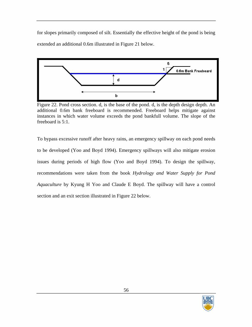
for slopes primarily composed of silt. Essentially the effective height of the pond is being

extended an additional 0.6m illustrated in Figure 21 below.

Figure 22. Pond cross section. d, is the base of the pond. d, is the depth design depth. An additional 0.6m bank freeboard is recommended. Freeboard helps mitigate against instances in which water volume exceeds the pond bankfull volume. The slope of the freeboard is 5:1.

To bypass excessive runoff after heavy rains, an emergency spillway on each pond needs

to be developed (Yoo and Boyd 1994). Emergency spillways will also mitigate erosion

issues during periods of high flow (Yoo and Boyd 1994). To design the spillway,

recommendations were taken from the book Hydrology and Water Supply for Pond

Aquaculture by Kyung H Yoo and Claude E Boyd. The spillway will have a control

section and an exit section illustrated in Figure 22 below.

57

Figure 23. Emergency spillway. The emergency spillway consists of a level control section 6m in length. Excess flow will then discharge through the exit section and into the stream. The control section of the emergency spillway will be a flat section at least 6m in length

and will be lined with natural grass (Yoo 1994). The maximum depth of flow in this

section will be at least 0.3m (Yoo 1994). The cross section of the spillway will be

rectangular in shape, although an additional freeboard of 0.3m at a slope of 5:1 towards

the control section will be added (Yoo 1994). Flow from the control section of the

spillway will then discharge into the exit section. The exit section will be lined with

natural grass and have a gentle slope of 5:1 until it discharges into the stream system. The

width of the control section and exit section will be the same as the initial width of the

most upstream portion of the stream which is determined in Phase 3.

The pipe which discharges rooftop runoff will need to be appropriately sized. At this time

proper pipe sizing has not been conducted due to the unavailability of South Campus

Neighbourhood rooftop data. Details on pipe sizing will be conducted in Phase 5. The

depth the pipe enters the pond is dependent on a variety of factors and will be further

58

investigated in Phase 4. The pipe should extend no further than 1/3 the length of pipe into

the pond (Schwab et al. 1981). The area of pond directly influenced by the pipe discharge

should be lined with riprap to prevent murky water created by silt disturbance (Schwab et

al. 1981). The Vancouver Building Code designs rooftop drainage systems to be able to

handle a rainfall event of 15minutes which may occur once every 10 years (BC Building

Code 2000). This corresponds to a rainfall intensity of 35mm/hr (Appendix I). The pipe

which collects rooftop runoff will be designed to handle a flowrate of at least 35mm/hr.

Vegetation along the banks of the ponds will increase aesthetics and bank stability (Donat

1995). It is important that this vegetation be able to survive during wet and dry periods

(Adams 1997). Vegetation will also provide oxygen to the ponds which will mitigate the

formation of anoxic conditions (Adams 1997). Ideal vegetation commonly seen near

ponds include: Irises, Narrow Leaf Cattail, Softrush, and Stem Bullrush (Adams 1997).

These are displayed in Appendix J.

59

PHASE 4: STREAM DESIGN AND DIMENTIONING

The novelty of this study is to design a stream suited to fish habitat requirements as well

as being able to manage stormwater. The stream will manage stormwater by conveying

overflow from each pond downstream towards the Pacific Ocean. To ensure the stream

conforms to the target species habitat requirements, design took into consideration the

following:

Fish Habitat Considerations

Proper placement and spacing of cascade pool and riffle pool sequences.

Randomization of cascade, riffle and pool spacing. This ensures a natural looking

stream. Spacing typically varies from 6 to 8 times the bankfull width (Newbury et

al. 1997).

Degree of meandering (typically 8 to 12 times the bankfull width) and radius of

curvature (Leopold et al. 1964).

The bankfull width to cascade/riffle depth ratio should lie between 5 to 1 and 10

to 1 to maintain good habitat (Hunter 1991).

In stream pools will hold a minimum volume of 1m3 (Hunter 1991). This will

ensure adequate depth for fish refuge and ensure pond areas do not dry out easily

during dry periods.

Stream velocities will not exceed the critical swimming velocity of ~1m/s (Dane

1978).

60

Stream velocities maintain cobble and gravel on the stream bed. Cobble and

gravel are characteristic stream bed material found in natural cascade pool and

riffle pool sequences (Hogan and Ward 1997). Smaller sediment which is abrasive

to fish gills and eggs will be transported out of the stream system.

If possible a summer time depth of 0.06m should be maintained (Whyte et al.

1991).

Sufficient bank side vegetation for food, cover, and slope stability (Hunter 1991).

Additional Considerations

The flowrate should increase from upstream to downstream.

To ensure downstream portions of the stream are able to handle upstream flow

contributions, the width of the stream will gradually increase from upstream to

downstream.

To mitigate the effects of periods of high flow, the stream banks will have an

additional freeboard bank height of 0.3m which slopes towards the stream at a 3:1

slope.

The location of riffle and cascade pool stream morphology was discussed in Phase 1 and

is illustrated in Figure 19. Typical cascades and riffles are spaced 6 to 8 times the

bankfull width apart from instream ponds (Leopold et al. 1964). To ensure a natural

looking stream, a randomization function was utilized using Microsoft Excel. The results

are displayed in Appendix K. To achieve sufficiently sinuous stream, the degree of

61

meandering typically occurs at 8 to 12 times the bankfull width with a curvature of radius

at approximately 2.3 (Leopold et al. 1964). The degree of meandering would normally be

determined with the use of a random generator to simulate a natural environment. Since

space is limited it may not be feasibly to randomize meandering. Appendix L displays the

results of a random generator for meandering. The degree of meandering and curvature of

radius will be determined after a survey has been done along the edge of Pacific Spirit

Regional Park to best determine how much space is available for meandering.

The stream was divided into fourteen sections based on the contour lines on a topography

map of the south campus area. These fourteen sections were labeled A to N and are

displayed in Appendix M. The slope of each section was determined (Appendix N).

Areas with slopes less then 2% were designed to have riffle pool morphology, while

slopes between 2% and 5% were designed to have cascade pool morphology. Riffle

portions of the stream will have a stream bed primarily made up of gravel which has a

diameter ranging from 2 to 64mm (Arcement and Schneider 2005). Cascade portions of

the stream will have a stream bed primarily made up of cobble and gravel. Cobble varies

in diameter from 64mm to 256mm (Arcement and Schnieder).

The chosen channel morphology is flat bottomed with vertical sides (Figure 23). This

type of morphology will become more rounded as the stream matures. It will also

promote the formation of undercut banks which are ideal for fish refuge (Appendix O).

An additional freeboard bank height of 0.3m sloping towards the stream will be placed on

62

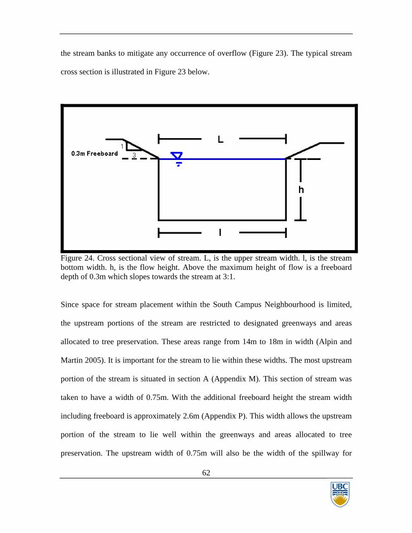
the stream banks to mitigate any occurrence of overflow (Figure 23). The typical stream

cross section is illustrated in Figure 23 below.

Figure 24. Cross sectional view of stream. L, is the upper stream width. l, is the stream bottom width. h, is the flow height. Above the maximum height of flow is a freeboard depth of 0.3m which slopes towards the stream at 3:1. Since space for stream placement within the South Campus Neighbourhood is limited,

the upstream portions of the stream are restricted to designated greenways and areas

allocated to tree preservation. These areas range from 14m to 18m in width (Alpin and

Martin 2005). It is important for the stream to lie within these widths. The most upstream

portion of the stream is situated in section A (Appendix M). This section of stream was

taken to have a width of 0.75m. With the additional freeboard height the stream width

including freeboard is approximately 2.6m (Appendix P). This width allows the upstream

portion of the stream to lie well within the greenways and areas allocated to tree

preservation. The upstream width of 0.75m will also be the width of the spillway for

63

Pond 1 and Pond2. At the recommended width to depth ratio of 5:1, the depth of the

stream in Section A was determined to be 0.15m (Appendix Q). This depth is well above

the minimum required depth of 0.06m during summer periods.

In each section, the average flow rate of the stream was determined through application

of the Manning’s equation displayed below.

Units)SI(,121

32

nSARQ = Equation 1

Where,

Q, is flowrate of the stream in m3/s.

A, is cross sectional area of the stream in m2.

S, is channel slope.

R, is the hydraulic radius of the channel (m), and can be defined as

the channel area divided by the wetted perimeter.

n, is roughness coefficients which vary depending on the channel

conditions.

The Manning’s equation was not applied to the pond portions of the stream. This is

because the ponds are considered deep and essentially have a velocity of zero in

comparison to the cascade and riffle portions of the stream.

64

The Manning’s coefficient was determined using the procedures outlines in Appendix R.

The method outlined by Arcement and Schneider, takes into consideration channel

irregularities, variation in channel cross-section, effects of obstruction, effects of

vegetation, and the degree of meandering. The table below illustrates the contribution of

each of these effects to the Manning’s Roughness coefficient. For many of these

coefficient values, a range was given. The lower and upper ranges of these values were

taken to determine the lower and upper Manning’s roughness coefficient values for

gravel and cobble lined streams. This allowed a sensitivity analysis to be conducted to

determine the effect of Manning’s roughness coefficient on stream flowrate.

Table 4. Manning’s Roughness Coefficients. The upper and lower Manning’s coefficient values for gravel and cobble are highlighted below.

Manning's Roughness Gravel Cobble

Coefficients Low Upper Low Upper

nb: base value 0.028 0.035 0.030 0.050

n1: channel irregularities 0.001 0.005 0.001 0.005

n2: variation in channel x-sec 0 0 0 0

n3 effect of obstruction 0.005 0.015 0.005 0.015

n4 effect of vegetation 0.002 0.010 0.005 0.010

m: degree of meandering 1.150 1.150 1.150 1.150

n=(nb+n1+n2+n3+n4)m 0.041 0.075 0.047 0.092

Gravel attained a lower Manning’s coefficient value of 0.041 and an upper value of 0.075.

Cobble had a lower Manning’s coefficient value of 0.047 and an upper value of 0.092.

65

The average flowrate of each stream section was then determined using the upper and

lower Manning’s coefficients. Important parameters of each stream section were

tabulated in Microsoft Excel. Figure 24 below illustrates and example of this tabulation.

Figure 25. Sample tabulation of stream section A. The chart to the left utilizes the lower end Manning’s coefficient value, while the chart to the right utilizes the upper end Manning’s coefficient value. The effects of varying Manning’s coefficient on flowrate could then be directly compared.

To ensure the downstream portions of stream had a higher flowrate than the upstream

sections, stream depths and widths were varied accordingly with the design

considerations in mind (Appendix S). Pool depth was varied to ensure a volume of at

least 1m3. The recommended stream dimensions are outlined in Appendix T. Note that

these dimensions will change depending on the current conditions.

66

It is important to note that any additional input of flow into the stream will increase the

overall stream flow. For example, in section D the riffle pool portion of the stream will

receive flow from the Pond 2 spillway during periods of pond overflow. The stream must

be designed to be able to handle this additional flow. Thus the rate of flow in section D

includes the additional flow from the Pond 2 spillway. This addition increases the overall

dimensions of the stream. If at any section additional flow is diverted into the stream, the

dimensions of the section and those downstream of it must be adjusted to be able to

manage the additional flow.

Using the lower end Manning’s roughness coefficient the furthest upstream flowrate is

0.10m3/s with a velocity of 0.87m/s (Appendix T). The furthest downstream portion has a

flowrate of 0.70m3/s and a velocity of 1.30m/s (Appendix T). Using the upper end

Manning’s roughness coefficient, the furthest upstream flowrate is 0.05m3/s with a

velocity of 0.45m/s (Appendix T). The furthest downstream portion has a flowrate of

0.36m3/s and a velocity of 0.66m/s (Appendix T). The streambed will be lined with

gravel in the riffle pool section and predominantly cobble in the cascade-pool sections

since these sediments are ideal for salmon spawning. Cobble has a diameter of 64mm to

256mm and gravel has a diameter ranging from 2mm to 64mm. Ideal substrate size for

cutthroat is 6mm to 102mm (Whyte et al. 1991).

The upstream and downstream velocities determined using the lower and upper end

Manning’s roughness coefficients will promote the sedimentation of gravel and cobble.

67

Smaller streambed material will either be transported or eroded away. This is illustrated

in Figure 25 below.

Figure 26. Critical velocity with respect to streambed material (sediment) diameter. The vertical green lines indicate the range of gravel size from 2mm to 64mm. The vertical red lines indicate the range of cobble size from 64mm to 256mm. The horizontal pink lines indicated the highest velocity of 130cm/s and the lowest velocity of 87cm/s attained using the lower end value of Manning’s roughness coefficient. The horizontal blue lines indicate the highest velocity of 66cm/s and the lowest velocity of 45cm/s attained using

68

the upper end value of Manning’s roughness coefficient. Where the horizontal lines cross with the vertical lines, indicate the transport zone the stream bed is experiencing.

Figure 26 indicates that the majority of gravel and cobble material will undergo

sedimentation and remain on the streambed. Smaller diameter sediment will be

transported or eroded downstream. When velocities reach greater than 16cm/s the smaller

diameter gravel material erode or transport downstream. From the figure it appears that

over time the stream bed will predominantly be made of sediment with a diameter greater

than 10mm. This is ok since the majority of the stream is cobble pool sequence and since

ideal sediment size for the target species is between 6mm and 102mm.

69

PHASE 5: PIPING DISTRIBUTION SYSTEM DESIGN

A detailed design of the piping distribution system was unable to be conducted. This was

due to time limitations and the inability to receive information on the buildings which

will be constructed on the South Campus Neighbourhood. It will be assumed that the

buildings on South Campus conform to the British Columbia Building Code and are thus

designed to handle a one in 10 year storm event which lasts 15minutes. This corresponds

to a flowrate of 35mm/hr or 61072.9 −× m/s. Focus will be placed on the important design

considerations of a pipe which collects stormwater at a rate of 61072.9 −× m/s and

conveys flow into the ponds.

Four important design considerations which will be discussed include:

Outlet Type

Pipe Depth

Pipe Size

General Design and Layout Procedures

The two major types of outlets include gravity and pump outlets (Schwab et al. 1981).

Pump outlets require the use of a pump to convey water through the outlet and are

typically used when the water level at the outlet is greater than the bottom of the pipe

outlet for an extended period of time (Schwab et al. 1981). Gravity outlets are more

70

common and simply use the force of gravity to transport water (Schwab et al. 1981).

Common design recommendations include:

A minimum distance of 30cm between the pipe outlet and water level of the pond.

The length of the outlet should not extend over 1/3 of the pipe length.

The pipe should be made out of a metal material and have a minimum length of

5m.

The addition of a flap, grid, or tide gate on the outlet to prevent rodents from

entering the pipe.

(Schwab et al. 1981)

These design recommendations are illustrated in Appendix U.

A properly designed outlet should provide a free outlet with minimum maintenance,

discharge outflow without erosion or damage to pipe, keep out rodents and small animals,

prevent the end of the outlet from excessive freezing and thawing, and prevent the

entrance of during periods of high flow (Schwab et al. 1981).

.

The depth of the pipe depends on soil permeability, outlet depth, lateral spacing, depth to

the impermeable layer in the subsoil, and limitations of excavation equipment. Pipe depth

is defined as the distance from the surface to the bottom of the pipe. The cover over the

pipe should be at least 60cm (Schwab et al. 1981). This will protect the pipe from heavy

71

surface loads. If the pipe is placed at a depth below an impermeable layer, then

backfilling should be done with permeable soil. (Schwab et al. 1981)

The size of the pipe will vary depending the drainage coefficient (term used for velocity),

drainage area, pipe roughness, and the slope of the terrain. Basic drain size can be

determined using the following formula:

1875.0375.0)(7.51 −××××= snADd c

Where,

d, is inside drain diameter in mm

Dc, is drainage coefficient in mm/d

A, is drainage area in hectares

n, is Manning’s roughness coefficient

s, is the drain slope

(Schwab et al. 1981)

A nomograph is often used in pipe sizing but will not be discussed.

When designing the layout of a pipe distribution system, the system needs to be

coordinated with existing and proposed drains. Procedures include preliminary surveys of

the area, soil investigation to determine practicality and economic feasibility, and the use

of topography maps. In general, the British Columbia Building Code for pipe

distributions systems and drainage will need to be followed.

72

5.0 RESULTS AND DISCUSSION With the addition of the pond and stream system, post development runoff volumes

differed from pre development runoff volumes by an average of 15% (Appendix V).

Without the pond and stream system, the post development runoff volumes differed from

the pre development runoff volumes by 21% (Appendix V). Thus, the addition of the

pond and stream system will decrease the level of runoff volume by approximately 6%.

These values were determined by averaging the results attained using the lower and upper

Manning’s coefficients. This 6% improvement corresponds to a reduced runoff volume of

134m3 during a 15minute, one in 10 year storm event. Although the post development

runoff volumes did not equal the predevelopment runoff volumes, the 6% decrease in

runoff volume is a significant step towards achieving post development runoff volumes

which roughly equal predevelopment runoff volumes.

The pond and stream system was unable to limit the total runoff volume to 10% or less of

the total rainfall volume. The pond and stream system was only able to limit the total

runoff volume to approximately 78% of the total rainfall volume (Appendix V). This

guideline may have been difficult to achieve since the pond and stream system is only

taking runoff from a small area of rooftops in comparison to the large area which makes

up the South Campus Neighbourhood. If only the immediate area surrounding the pond

and stream system were considered, then the total runoff volume would be closer to the

goal of 10% or less of the total rainfall volume.

73

A pond and stream model, which is supported by rooftop runoff, was able to be

developed through the use of fluid mechanics and the consideration of fish habitat. The

consideration of fish habitat made this study a novel approach towards better stormwater

management.

The use of two ponds to collect rooftop runoff enhanced the stormwater management

capabilities of the pond and stream system. This is because the ponds are able to handle a

large volume of rooftop runoff before discharging flow into the stream system. It was

found that Pond 1 could manage 17 150m2 rooftop area and Pond 2 can manage 7891m2

rooftop area (Appendix W). This was done by assuming the ponds were full from a storm

event, and proceeding to fill from the occurrence of a 15minute storm event which occurs

once every 10years. The flowrate into the Pond 1 spillway had to be less than the

upstream portion of the stream, while the flowrate into the Pond 2 spillway had to be less

than the flowrate in Section D of the stream. The corresponding area of rooftops the pond

and stream system could handle were then determined (Appendix W). The actual area of

the rooftops which will reside in the South Campus Neighbourhood is unknown. These

areas are large considering a typical lot in the area is 5 000m2. The addition of ponds

should greatly reduce the demand on any artificial stormwater structure which may be in

place. The ponds are able to hold a volume of 152m3. At an average rainfall intensity of

0.017m/day for the month of November, it was found that each pond would take

approximately 10 days of steady rain to fill (Appendix X). Any excess volume would be

discharged into the spillway. The pond will also lose volume through infiltration.

Infiltration is dependent on the hydraulic conductivity of a soil. If the hydraulic

74

conductivity of the pond material is too high, the pond will be unable to maintain a base

flow. The ponds were designed to have a depth of 1.5m since this depth remained in the

silt matrix layer of the soil. If the depth proceeded past approximately 2-3m, then the

pond would reach the sandy layers of soil and loss through seepage would be fast. Phase

3 further describes in detail the design and dimensioning of the ponds.

Stream design took into consideration major urban stream issues such as overflow,

erosion, and periods of high and low flow. The design of the stream did not consider

infiltration. This was to design the stream under a conservative approach to take

maximum flow conditions into consideration. To mitigate rare occurrences of overflow,

the stream banks were designed to have an additional freeboard height of 0.3m sloping at

3:1 towards the stream. The stream was designed to prevent erosion by designing the

stream for velocities which promote the sedimentation of cobble and gravel, which are

suited to the target fish species. Smaller particles which may be abrasive to fish eggs or

gills would be transported down stream. In addition, vegetation should be planted on the

stream banks to further protect against erosion. The stream will experience variable

periods of high flow during the winter months and low flow during the summer months.

To determine how variable the flow is, it will be important to excavate into the stream

location to determine how much base flow may be possible through ground water

seepage. The final stream design had a maximum width of 1.8 meters at the downstream

portion of the stream and a depth to width ratio of 1:6 (Appendix T). This lies well within

the requirement for good habitat which typically has a depth to width ratio of 1:5 to 1:10.

Thus, the stream could become larger to accommodate the input of additional flow if

75

needed. If the stream is sized to become larger, the designer needs to consider space

availability and whether or not the culvert which crosses Southwest Marine Drive can

handle the flow. The stream becomes wider from upstream to downstream and the

flowrate through the stream increases from the upstream to downstream (Appendix T).

This ensures the downstream portions of the stream are able to handle the flow

contribution from the upstream portion. Any additional flow from sources not considered

to have good water quality will have to be treated. The method of treatment will warrant

investigation and vary depending on the type of contaminants which may be present.

Stream velocities using the lower end Manning’s coefficient ranged from 0.87m/s to

1.29m/s (Appendix T). Stream velocities using the higher end Manning’s coefficient

ranged from 0.45m/s to 0.66m/s (Appendix T). Stream velocities at using the low end

Manning’s coefficient slightly exceeded the maximum swim velocity of 1m/s for

cutthroat trout. It is recommended that the stream be designed to have a Manning’s

coefficient closer to the higher end Manning’s coefficient. The higher end Manning’s

coefficient provided ideal stream velocities for the target species. Manning’s roughness

coefficient can be increased through increased stream complexity. This includes the

addition of structures such as large woody debris and vegetation.

A survey along Pacific Spirit Regional Park will need to be conducted to determine how

much space is available for meandering. The random generated chart in Appendix L can

be used, although it is recommended that meandering be varied based on field

76

observations due to the limited space availability. Additional details on stream design and

dimensioning are discussed in the Phase 4 portion of the report.

Unfortunately due to the inability to receive sufficient information on the buildings which

will be constructed on the South Campus Neighbourhood, a piping distribution system

was unable to be developed at this time.

It is difficult to predict whether the stream will be able to maintain a base flow

throughout the year. During the months of high precipitation (October to May), it is

expected that the stream will be able to maintain a base flow. This cannot be guaranteed

during the summer months. Since little precipitation is received during the summer

months, it is likely that the ponds will become completely dry. This will be acceptable

since it will prevent any type of mosquito problem which may occur. It is recommended

that if the stream system is applied, it be allowed to function under continual monitoring

to determine seepage rates into the stream and how well the system is functioning. Once

the system is determined to be functioning properly then fish may be reintroduced.

77

6.0 CONCLUSION AND RECOMMENDATIONS

A design methodology which can be used to develop a pond and stream system suitable

for South Campus and fish habitat was developed. This methodology may be used as a

template whenever the restoration of a stream is being considered as an option to manage

urban stormwater runoff.

With the addition of the pond and stream system, post development runoff volumes

differed from pre development runoff volumes by an average of 15%. Although the post

development runoff volumes did not equal the predevelopment runoff volumes, the 6%

decrease in runoff volume is a significant step towards achieving post development

runoff volumes which roughly equal predevelopment runoff volumes. The pond and

stream system was unable to limit the total runoff volume to 10% or less of the total

rainfall volume. The pond and stream system was only able to limit the total runoff

volume to approximately 78% of the total rainfall volume. This guideline may have been

difficult to achieve since the pond and stream system is only taking runoff from a small

area of rooftops in comparison to the large area which makes up the South Campus

Neighbourhood.

The pond and stream model was able to be developed through the application of fluid

mechanics and the consideration of fish habitat. In addition, major urban stream issues

were addressed. Unfortunately a proper piping distribution system which will discharge

rooftop runoff into the ponds was able to be developed. This is something which can be

developed in the future once the required information is available.

78

It is important to note that this study provides a methodology outlining key design

considerations when attempting to design a pond and stream system which manages

stormwater runoff while taking fish habitat criteria into consideration. Before the

methodology is carried out, the following recommendations for future work should be

considered:

Excavation at various locations along the stream path to determine how much

base flow can be achieved.

Percolation tests need to be conducted to determine the hydraulic conductivity of

the soil. More accurate seepage rates can then be attained.

Survey of the land bordering Pacific Spirit Regional Park. This will determine the

amount of available space for stream meandering.

Once the necessary building structure information is attained, a proper piping

distribution system can be constructed to convey stormwater runoff from

rooftops to the ponds.

If the stream is put in place, allow it to run for a few years. During this time

periodic monitoring will allow seepage rates into the stream to be determined.

Detailed cost analysis to determine the feasibility and possible cost savings of

implementation of this methodology.

Implementation of such a project involves the considerations of all stakeholders,

which may be influence. A multidisciplinary approach is necessary to achieve

success and ensure all concerns are addressed.

79

RESEARCH IMPLICATIONS The possible implication of this study is that an urban stream which manages both

stormwater and fish habitat criteria flow through the University of British Columbia

campus, restoring the fish bearing stream which previously existed. The aim is for fish to

one day utilize the stream as habitat and spawning areas. Implementation of the stream

and pond system will also help the University of British Columbia to strive towards

meeting federal and provincial stormwater management guidelines. On a larger scale, the

research promotes sustainability through fish habitat conservation, reduced peak runoff

flows, and efficient use of water resources.

80

ACKNOWLEDGEMENTS

I would like to thank the following people for their contributions towards this study. Dr. Petrell – Thesis Advisor - For her time, contribution, patience, and faith in me to undertake this project. Brenda Sawanda – UBC Sustainability Office - For her contribution and enthusiasm for the project. David Grigg – Associate Director Infrastructure and Services Planner UBC - For his time and input into the project. Bianca Gunther – Geography - For her contribution through her GPS and mapping abilities. Rob Little and Carolina Silva – Economic Analysis - For conducting cost analysis on the feasibility of the project.

81

REFERENCES Arcement GJ and Schneider VR. 2005. Guide for Selecting Manning’s Roughness Coefficients for Natural Channels and Flood Plains. United States Geological Survey Water-supply Paper 2339. 67 pp Adams M. 1997. Fish Habitat Enhancement: A manual for Freshwater Estuarine and Park Habitat. Department of Fisheries and Oceans. 324 pp Aplin and Martin Consultants LTD. 2005. A Sustainable Drainage Strategy for the South Campus Neighbourhood. 30 pp British Columbia Building Code. 2000. City of Vancouver. Pp British Columbia Ministry of Environment. 2002. Stormwater Planning Guidbook: Policies for Integration of Land Use Planning and Stormwater Management Chapter 4. 17pp Coduto D.P. 1999. Geotechnical Engineering: Principles and Practices. Prentice Hall. Upper Saddle River. 759 pp Cowan W. L. 1956. Estimating hydraulic roughness coefficients. Agricultural Engineering, Vol 37, no. 7, pp 473-475 Dane B.G. 1978. A review and resolution of fish passage problems at culvert sites in British Columbia 4th Edition. Department of Fisheries and Environment, Pacific Region, Fisheries and Marine Service Technical Report No. 810. pp 126 Department of Fisheries and Oceans (DFO). 2005. http://www.dfo-mpo.gc.ca/ Accessed November 2005 Donat M. 1995. Bioengineering Techniques for Streambank Restoration: A Review of Central European Practices. Finkenbine J. 1998. The impact of urbanization on stream habitat in Lower Mainland British Columbia. University of British Columbia Finnemore E.J. and Franzini J.B. Fluid Mechanics with Engineering Applications 10th Edition. McGraw Hill. New York. 790 pp

82

Freeman, G.E.1994. The Scientific Assessment and Strategy Team Contributions Assessing the 1993 Flood on the Mississippi and Missouri River Basins. Water International, 19 (1994) 177-185, International Water Resources Assoc., USA. Hogan D.L. and Ward B.R. 1997. Watershed Geomorphology and Fish Habitat. Fish Habitat Rehabilitation Procedures. Chapter 2 pp 2-1: 2-18 Hunter C.J. 1991. Better Trout Habitat: A Guide to Stream Restoration and Management. Island Press. New York. 320 pp Huth M.J. 1978. The urban habitat: past, present, and future. Nelson-Hall Chicago Johnston N.T. and Slaney P.A. 1996. Fish Habitat Assessment Procedures. Watershed Restoration Technical Circular No. 8 Ministry of Environment, Lands and Parks and Ministry of Forests. pp 97 Lane EW. 1955. Design of Stable Channels. Trans. A.S.C.E., Vol. 120 Lencastre A. 1987. Handbook of Hydraulic Engineering. Ellis Horwood Limited. 540 pp Leopold L.B., Wolman M.G., and Miller J.P. 1964. Fluvial processes in geomorphology. Freeman, San Francisco, CA. 522pp Martin V. 1996. Velocity Structure in Gravel Rivers. University of British Columbia Graduate Thesis. pp 29-35 Ministry of Environment, Lands, and Parks and Ministry of Forests (MELP and MF). 1999. Fish Passage-Culvert Inspection Procedures. 50pp Ministry of Water, Land, and Air Protection (MWLAP) British Columbia. 2004. Standards and Best Practices for Instream Works. 174pp Moyle P.B., Cech JJ. 2004. Fishes: An Introduction to Ichthyology 3rd Edition. Prentice Hall Inc. 590 pp Murray and Associates. 2005. South Campus Neighbourhood Subdivision Plan. 1pp Naturegrid. 2005. http://www.naturegrid.org.uk/rivers/watercyclepages/riverbasin-stages.html Accessed November 2005 Neill C.R. 1967. Mean Velocity Criterion for Scour of Course Uniform Bed Material. Proc., 12th Congress of IAHR, Fort Collins.

83

Newbury R., Gaboury M. Bates D. 1997. Restoring Habitats in Channelized or Uniform Streams Using Riffle and Pool Sequences. Fish Habitat Rehabilitation Procedures. Chapter 12 pp 1-22 Petrell R. 2005. Consultation through weekly meetings. September 2005 to April 2006 Sherwood J.M. 1994. Estimation of peak-frequency relations, flood hydrographs, and volume – duration – frequency relations of ungaged small urban streams in Ohio. U.S. Geological Survey water – supply paper: 2431 Simon Fraser University (SFU). 2006. Watercourse and Stormwater Management Plan for Burnaby Mountain. http://www.univercity.ca/bmcp/swmexecutivesummary.html Accessed February 2006 Schwab G.O., Frevert R.K., Edminster T.W., Barnes K.K. 1981. Soil and Water Conservation Engineering 3rd Edition. John Wiley & Sons Inc. New York. 525 pp University of British Columbia (UBC). 2004. South Campus Northeast Sub-Area Neighbourhood Plan. pp 53 U.S. Soil Conservation Service. 1974. Handbook of Channel Design for Soil and Water Conservation. USDA Forest Service. 2005. http://www.fs.fed.us/ Accessed November 2005 Ven Te C. 1981. Open-channel Hydraulics. McGraw-Hill. New York. 123 pp

Yoo KH and Boyd CE. 1994. Hydrology and Water Supply for Pond Aquaculture. Chapman and Hall. New York. 483 pp

Ministry of Environment (MOE). 1991. Manual of Operational Hydrology in British Columbia Second Edition. Pg 149

84

APPENDICES

85

APPENDIX A: TOPOGRAPHY MAP OF SOUTH CAMPUS The blue lines outline the roads which boarder and lie within the South Campus Neighbourhood plan. The contour lines of the map indicate that the land slopes in a southeasterly direction. This played a factor when deciding the ideal stream location. The red ovals indicate pond locations, while red arrows indicate the recommended path of stream flow. Contour lines on the map are space by increments of 5feet.

86

APPENDIX B: AERIAL PHOTOGRAPH OF SOUTH CAMPUS The yellow line outlines the south campus area of the University of British Columbia. The broken black line outlines the South Campus Neighbourhood. The red oval indicates the area to the west of the South Campus Neighbourhood. This area is currently used for agricultural research making it difficult to allow a stream to flow through this area.

(Alpin and Martin 2005)

87

APPENDIX C: SOUTH CAMPUS LAND USE PLAN The land use plan for the South Campus Neighbourhood. The stream was limited to areas designated as greenways (including UNOS areas) and land allocated to tree preservation and management.

88

APPENDIX D: RATIONAL FORMULA RUNOFF COEFFICIENT, C TABLE The terrain of south campus was considered moderate and the design rainfall intensity is a 15minute storm event, which occurs once every 10 years. Predevelopment is forested and will then have a runoff coefficient of 0.67. Post development is urbanized and will thus have a runoff coefficient of 0.85.

(MOE 1991)

89

APPENDIX E: PONDS, STREAM, AND CULVERT PLACMENT Pond 1 lies in the UNOS area SC2H and Pond 2 lies in UNOS area SC3G. Each pond is indicated by a blue oval. The yellow stars indicate locations where culverts are needed to allow the stream to cross roads. The arrows illustrate the flow path of the stream.

90

APPENDIX F: SOUTH CAMPUS NEIGHBOURHOOD SUBDIVISION PLAN Pond 1 lies in the UNOS area SC2H and Pond 2 lies in UNOS area SC3G. These designated green spaces provide adequate area for Pond placement. UNOS area SC2H encompasses 4320.7m2 of land, while UNOS area SC3G encompasses 6796.7m2 of land. (Murray and Associates 2005)

91

92

APPENDIX G: SAMPLE BOREHOLE RESULT This is a typical borehole result done in the SC3D plot of the South Campus Neighbourhood. Till primarily composed of silt reaches depths of approximately 3.5m. Below this depth lies sand.

(GeoPacific Consultants Ltd 2005)

93

APPENDIX H: SAMPLE POND DIMENSION CALCULATIONS The ponds will have the following dimensions:

Figure 20. Pond dimensions. Aerial view of pond. The base of the ponds have a length of 5m and a width of 1.5m. The total length of the pond is 20m and the total width is 16.5m. The side slopes of the pond are 5:1. Since the sediment within the pond is primarily silt, the 5:1 side slopes will provide adequate stability.

Calculation 1: Surface area of the pond base and surface. The surface area of the pond base and surface is oval in shape. The equation for the surface area of an oval is:

Π××= 2W

2L Surface Pond of Area Surface

Where, L, is the length of the pond surface or base W, is the width of the pond surface or base Π , is Pi

94

Thus,

2260 25.16

220m Surface Pond of Area Surface mm

=Π××=

29.5 25.1

25m Base Pond of Area Surface mm

=Π××=

The ponds are essentially oval frustums. To simplify calculations, oval frustums can be looked at as horizontally compressed circular frustums. An oval and circular frustum are displayed below.

To determine pond volume and the wetted surface area, the oval frustum must be reformed into a circular frustum. This is done by determining the surface area of the top and bottom of the oval ponds. To determine the corresponding circular frustum the following can be followed: Determine the surface area of the upper and lower oval frustum. Place this area in the equation for the area of a circle.

1.37m equal willandmanner.similar ain determined be alsocan pond theof base for ther

circle.upper frustums circle ingcorrespond theof radius theis 9.1mR r,for Solve

260r Circle Area260m Frustum Upper of Area Surface

22

2

=

=Π=

=

m

95

The volume of the circular frustum can then be determined.

( ) [ ] 32222FrustumCircular 152)37.1()37.108.9()08.9(

3)5.1(

3Volume mmmmmmrRrRh

=+×+Π

=++Π

=

The Area of the sides within a circular frustum is given by:

)( RlrlArea +Π= Since depth of the pond is known to be 1.5m, l, can be determined.

Note: d is depth = 1.5m, r is the pond base radius, R is the upper pond circle radius, l is the length of the sides. X needs to be found to determine l. mrRx 71.7=−= Thus, mmmxdl 85.7)71.7()5.1()( 2222 =+=+=

2258)85.708.985.737.1()( mmmmmRlrlArea =×+×Π=+Π= Typically want to know the total surface area the rain touches, thus must add the surface area of the base to the surface area of the sides. Thus 258m2 + 5.90m2 = 264m2

APPENDIX I: UBC RAINFALL IDF CURVES

96

The British Columbia Building Code states that rooftop drains are designed to handle a storm event which last 15 minutes and occurs once every 10 years. This corresponds to a rainfall intensity of approximately 35mm/hr, which is the intensity the pipe, which drains into the pond, will be designed to handle. The green arrows on the graph below indicate this.

(British Columbia Ministry of Environment 2002)

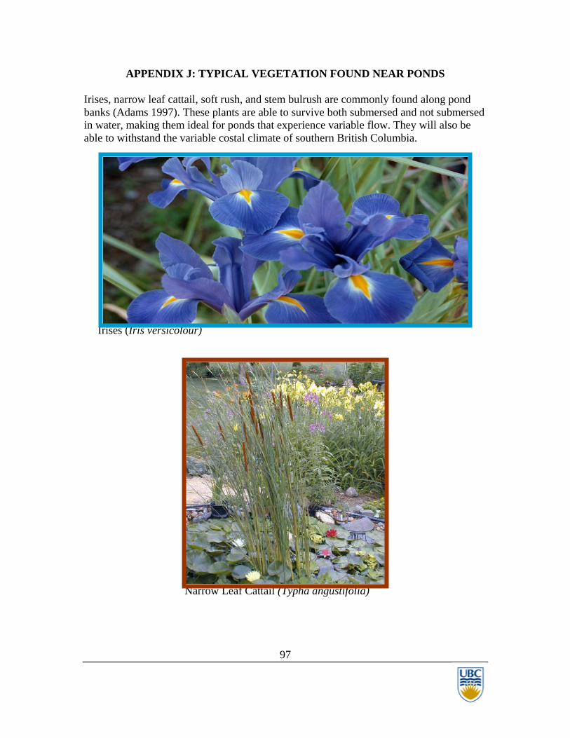
97

APPENDIX J: TYPICAL VEGETATION FOUND NEAR PONDS Irises, narrow leaf cattail, soft rush, and stem bulrush are commonly found along pond banks (Adams 1997). These plants are able to survive both submersed and not submersed in water, making them ideal for ponds that experience variable flow. They will also be able to withstand the variable costal climate of southern British Columbia.

Irises (Iris versicolour)

Narrow Leaf Cattail (Typha angustifolia)

98

SSoft rush (Juncus effuses)

Soft Stem Bulrush (Scirpus validus)

99

APPENDIX K: RANDOMIZATION OF CASSCADE POOL & RIFFLE POOLS The following table displays the results of the randomization trials. The results cut off when the section length is achieved. For example in section A will begin with a riffle 5.3m in length followed by a pool 6m in length. The excel function used was: =Int(RANDBETWEEN(60,85)/10)*Bankfull Width

Section A B C D E F G H I J K L M N Bankfull Width (m) 0.75 0.80 0.85 0.90 1.22 1.30 1.42 1.50 1.55 1.60 1.65 1.70 1.75 1.80Section Length (m) 91 61 61 152 114 64 91 110 91 125 128 146 134 114

cascade/riffle to pool spacing 5.3 5.6 5.1 5.4 7.3 7.8 8.5 9.0 10.9 12.8 9.9 10.2 10.5 10.8Note: 6-8 Time Bankfull Width 6.0 4.8 6.8 6.3 8.5 9.1 11.4 10.5 9.3 12.8 11.6 11.9 10.5 14.4 4.5 4.8 6.0 6.3 9.8 7.8 9.9 12.0 10.9 12.8 11.6 10.2 12.3 14.4 5.3 5.6 5.1 5.4 7.3 7.8 8.5 10.5 9.3 9.6 13.2 11.9 10.5 10.8 6.0 4.8 6.0 5.4 8.5 9.1 8.5 9.0 12.4 9.6 9.9 13.6 12.3 10.8 5.3 6.4 5.1 5.4 8.5 9.1 9.9 10.5 12.4 12.8 13.2 10.2 12.3 14.4 4.5 4.8 5.1 5.4 8.5 7.8 9.9 10.5 9.3 12.8 9.9 10.2 10.5 10.8 4.5 4.8 6.0 5.4 9.8 11.4 10.5 10.9 12.8 9.9 10.2 10.5 10.8 4.5 5.6 6.0 7.2 9.8 11.4 9.0 10.9 11.2 9.9 13.6 14.0 10.8 5.3 6.4 6.0 7.2 8.5 9.9 9.0 11.2 11.6 10.2 12.3 4.5 4.8 6.8 6.3 9.8 9.0 9.6 11.6 11.9 10.5 5.3 6.4 6.0 6.3 7.3 11.2 11.9 6.0 5.4 7.3 11.9 4.5 6.3 7.3 4.5 6.3 5.3 5.4 6.0 7.2 5.3 7.2 7.2 5.4 5.4 5.4 5.4 6.3 7.2

100

APPENDIX L: RANDOMIZATION OF DEGREE OF MEANDERING

The values indicate the length of a stream in a given section before a meandering should occur. Typically cascades pool morphology streams meander at a smaller curvature of radius. The excel function used was: =Int(RANDBETWEEN(80,125)/10)*Bankfull Width

Section A B C D E F G H I J K L M N Bankfull Width (m) 0.75 0.80 0.85 0.90 1.22 1.30 1.42 1.50 1.55 1.60 1.65 1.70 1.75 1.80Section Length (m) 91 61 61 152 114 64 91 110 91 125 128 146 134 114

Stream Meander Length 6.8 7.2 9.4 9.0 9.8 14.3 15.6 12.0 12.4 12.8 18.2 17.0 14.0 14.4Note: 8-12 Time Bankfull Width 6.8 9.6 8.5 8.1 14.6 10.4 17.0 12.0 12.4 17.6 16.5 13.6 17.5 18.0 6.0 7.2 6.8 9.0 9.8 13.0 14.2 18.0 17.1 19.2 16.5 15.3 21.0 18.0 6.8 6.4 6.8 7.2 12.2 13.0 15.6 18.0 15.5 16.0 16.5 15.3 17.5 14.4 7.5 8.8 7.7 9.0 14.6 14.3 17.0 16.5 15.5 19.2 13.2 15.3 17.5 21.6 7.5 6.4 7.7 10.8 9.8 13.0 12.8 15.0 12.4 16.0 14.9 17.0 15.8 18.0 7.5 8.0 9.4 9.0 12.2 13.0 14.2 15.0 15.5 17.6 14.9 13.6 15.8 14.4 6.8 6.4 7.7 9.0 11.0 14.3 17.0 12.0 14.0 16.0 18.2 20.4 19.3 14.4 8.3 9.6 9.4 10.8 11.0 10.4 15.6 15.0 12.4 14.4 16.5 20.4 19.3 18.0 8.3 8.0 6.8 8.1 14.6 13.0 14.2 12.0 12.4 14.4 16.5 20.4 17.5 21.6 6.8 8.0 10.2 7.2 14.6 10.4 11.4 18.0 17.1 19.2 14.9 17.0 21.0 19.8 7.5 7.2 9.4 7.2 11.0 11.7 17.0 12.0 17.1 17.6 13.2 17.0 19.3 18.0 7.5 6.4 9.4 9.9 13.4 13.0 12.8 15.0 17.1 19.2 16.5 13.6 17.5 16.2 8.3 8.0 6.8 9.0 13.4 14.3 11.4 18.0 12.4 12.8 13.2 20.4 14.0 16.2 9.0 8.8 6.8 9.0 14.6 14.3 12.8 15.0 12.4 19.2 13.2 20.4 19.3 19.8 7.5 7.2 8.5 7.2 12.2 15.6 11.4 12.0 15.5 12.8 19.8 20.4 15.8 18.0 9.0 8.8 7.7 9.0 14.6 11.7 11.4 13.5 18.6 14.4 18.2 17.0 21.0 16.2 6.8 8.8 6.8 7.2 13.4 10.4 11.4 16.5 15.5 14.4 18.2 17.0 21.0 21.6 6.0 7.2 6.8 8.1 9.8 15.6 15.6 16.5 14.0 16.0 19.8 18.7 21.0 19.8 9.0 6.4 10.2 10.8 11.0 15.6 12.8 12.0 14.0 16.0 13.2 18.7 17.5 14.4 6.8 8.0 7.7 8.1 13.4 11.7 11.4 15.0 12.4 16.0 16.5 20.4 15.8 19.8 8.3 8.0 10.2 9.9 11.0 13.0 12.8 13.5 14.0 12.8 19.8 17.0 21.0 16.2 8.3 6.4 6.8 7.2 12.2 14.3 11.4 13.5 14.0 16.0 16.5 13.6 21.0 16.2 7.5 8.8 6.8 8.1 12.2 13.0 11.4 13.5 18.6 12.8 19.8 18.7 15.8 21.6 6.8 6.4 6.8 9.0 13.4 10.4 15.6 18.0 12.4 16.0 14.9 17.0 17.5 21.6 6.0 6.4 8.5 10.8 9.8 10.4 15.6 18.0 12.4 17.6 13.2 17.0 14.0 16.2 8.3 8.8 8.5 9.0 13.4 14.3 12.8 16.5 14.0 17.6 16.5 17.0 17.5 16.2

101

APPENDIX M: TOPOGRAPHY MAP OF SOUTH CAMPUS AREA The stream was divided into 14 sections based on 10feet spacing of contour lines.

102

APPENDIX N: SLOPE CALCULATIONS

The channel slope was determined using a topography map of the south campus. The following formula was used to determine the slope of a given area:

%100LinesContour Between Distance

LinesContour Between DifferenceElevation ×=Slope

For example the slope in section A will be given by,

%3.3%100m91m 3A Section in Slope =×=

APPENDIX O: UNDERCUT STREAM BANK

Undercut stream bank, ideal for fish refuge. The undercut bank provides shade and cover for fish.

103

APPENDIX P: WIDTH OF STREAM WITH ADDITIONAL FREEBOARD

This illustration shows how the full bank width increases with the addition of freeboard. In this scenario, the addition of 0.3m freeboard adds 0.9m to the width of the stream on each side. This increases the total full bank width from 0.75m to approximately 2.6m.

APPENDIX Q: DEPTH TO WIDTH RATIO CALCULATION EXAMPLE Given a width of 0.75m and a depth to width ratio of 1:5, the corresponding width is simply 0.75m/5 = 0.15m.

104

APPENDIX R: DETERMINATION OF MANNING’S COEFFICIENT USING METHOD OUTLINED BY Arcement and Schneider 2005. The method outlined by Arcement and Schneider is an alteration of Cowan’s (1956) procedure. The equation used to determine Manning’s coefficient is:

n = (no + n1+ n2 + n3 + n4) m5 Equation 4

Where n values account for,

no , basic straight, uniform, smooth channel

n1 , corrects for surface irregularities

n2 , channel cross section shape and size

n3 , obstructions

n4, vegetation and flow conditions

m5 , meandering channel

A series of tables are given with varying values of n and m5, depending on the channel

characteristics. The following tables are taken directly from the article and illustrate what

choices must be made to determine a proper Manning’s coefficient. The chosen values

are then entered into Equation 4 to attain a Manning’s coefficient for the stream.

105

no , basic straight, uniform, smooth channel

n1 , corrects for surface irregularities

106

n2 , channel cross section shape and size

n3 , obstructions

107

n4, vegetation and flow conditions

m5 , meandering channel

108

APPENDIX S: STREAM FLOWRATE VERSUS DISTANCE DOWNSTREAM These charts illustrate an increase in flowrate the further downstream one proceeds.

Stream Flowrate versus Downstream DistanceUpper Manning's Coefficient

00.050.1

0.150.2

0.250.3

0.350.4

0 200 400 600 800 1000 1200 1400 1600

Distance Downstream, m

Flow

Rat

e Q

, m3 /s

Stream Flowrate versus Downstream DistanceLower Manning's Coefficient

00.10.20.30.40.50.60.70.8

0 200 400 600 800 1000 1200 1400 1600

Distance Downstream (m)

Flow

Rat

e Q

, (m

3 /s)

109

APPENDIX T: STREAM DIMENSIONING DATA The following tables illustrate the tabulated and calculated parameters of each stream section. It was designed with the following design considerations in mind: Proper placement and spacing of cascade pool and riffle pool sequences.

Randomization of cascade, riffle and pool spacing. This ensures a natural looking

stream. Spacing typically varies from 6 to 8 times the bankfull width.

Degree of meandering (typically 8 to 12 times the bankfull width) and radius of

curvature.

The bankfull width to cascade/riffle depth ratio should lie between 5 to 1 and 10

to 1 to maintain good habitat.

In stream pools will hold a minimum volume of 1m3 (Hunter 1991). This will

ensure adequate depth for fish refuge and ensure pond areas do not dry out easily

during dry periods.

Stream velocities will not exceed the critical swimming velocity of ~1m/s (Dane

1978).

Stream velocities maintain cobble and gravel on the streambed. Cobble and gravel

are characteristic streambed material found in natural cascade pool and riffle pool

sequences (Hogan and Ward 1997). Smaller sediment, which is abrasive to fish,

gills and eggs will be transported out of the stream system.

The flow rate must increase from the upstream to downstream to allow the stream

to downstream portions of the stream to be able to handle upstream portions.

Sufficient bank side vegetation for food, cover, and slope stability.

110

111

112

113

114

APPENDIX U: PIPE DISCHARGING INTO POND CROSS SECTION Discharge pipe design and recommendations.

115

APPENDIX V: GUIDLINE CONFORMATION CALCULATIONS

To determine if post development runoff volumes roughly equal pre-development runoff volumes the following approach will be used:

ntRunoffedevelopmeCStreamOutSffpmentRunofPostDevelo QQQ Pr≈− Where,

QPostDevelopmentRunoff, is the flowrate of runoff after the construction of the South Campus Neighbourhood takes place in m3/s. QStreamOutSC, is the flowrate of the stream leaving the South Campus Neighbourhood in m3/s. QPredevelopmentRunoff, is the flowrate of runoff before the construction of the South Campus Neighbourhood takes place in m3/s.

It is important to note that any flow which discharges through the stream is not considered runoff since the stream is considered a natural system (MWLAP 2004). This is why QStreamOutSC removes the total runoff created by the post development runoff.

The rational formula assumes that the ground is saturated and can then be used to determine runoff volume. The system is designed for the maximum 15mintute storm that occurs once every 10 years ( sm /1072.9 6−× ). Thus, multiplying the post development, stream, and predevelopment flowrates by 15 minutes (900 seconds) will give the corresponding volumes.

sQsQsQ ntRunoffedevelopmeCStreamOutSffpmentRunofPostDevelo 900900900 Pr ×≈×−×

siAcsQsAic hoodsNeighbourSouthCampuntedevelopmeCStreamOutShoddsNeighbourSouthCampupmentPostDevelo 900900900 Pr ×≈×−×××

)900301000)/1072.9(67.0()900/17.0()900301000)/1072.9(85.0( 26326 smsmssmsmsm ××××≈×−×××× −−

Thus,

ntRunoffedevelopmemfwithStreapmentRunofPostDevelo VV Pr≈

33 17642152 mm =

%Difference= %182152

17642152%100 3

33Pr =

−=×

−

mmm

VVV

mfwithStreapmentRunofPostDevelo

ntRunoffedevelopmemfwithStreapmentRunofPostDevelo

116

If the stream is not included then,

sQsQ ntRunoffedevelopmeffpmentRunofPostDevelo 900900 Pr ×≈×

siAcsAic hoodsNeighbourSouthCampuntedevelopmehoddsNeighbourSouthCampupmentPostDevelo 900900 Pr ×≈×××

)900301000)/1072.9(67.0()900301000)/1072.9(85.0( 2626 smsmsmsm ××××≈×××× −−

Thus,

ntRunoffedevelopmereamfWithOutStpmentRunofPostDevelo VV Pr≈

33 17642238 mm ≠

% Difference = %21%1002238

17642238%100 3

33Pr =×

−=×

−

mmm

VVV

mfwithStreapmentRunofPostDevelo

ntRunoffedevelopmemfwithStreapmentRunofPostDevelo

Percent runoff improvement with the addition of the stream system is then 21%-18%, which equals 3% improvement in runoff. The post development volume runoff with the stream system differs from the predevelopment runoff volume by 18%.

Note: Qstreamout is taken at the upstream portion of Section E, since this is the best representative flowrate out of the South Campus Neighbourhood. 0.17m3/s is the flowrate of Section E at the high Manning’s coefficient.

Using the low Manning’s coefficient, Qstreamout is 0.24m3/s. Applying the same method

above at this flowrate:

ntRunoffedevelopmemfwithStreapmentRunofPostDevelo VV Pr≈

33 17642022 mm ≠

% Difference = 12.8%

Thus, 21%-12.8% = 8.2% runoff improvement

Average % Difference = (18%+12.8%)/2=15.3%

117

Average Improvement = (3%+8.2%)/2 = 6%

Average Reduced Runoff Volume = %Improvement

33eampmentNoStrPostDevelo 134223806.0V nt %Improveme Volume Runoff Reduced Average mm =×=×=

To determine if the total runoff volume, with the addition of the stream and pond system, will be less than or equal to 10% of the total rainfall volume, the approach will be used:

Volume Stream - Volume Runoff CampusSouth Volume Runoff Total =

Or

StreamumesRunoffVolSouthCampu fVolumeTotalRunof V VV −=

)900ESection in t Coefficien sManning'Higher or Lower at Velocity ()900(V fVolumeTotalRunof ssAic ×−×××= At Low Manning’s coefficient,

)900/24.0()900301000)/1072.9(85.0(V 326 fVolumeTotalRunof ssmsmsm ×−××××= −

= fVolumeTotalRunofV 2022m3

At High Manning’s coefficient,

)900/17.0()900301000)/1072.9(85.0(V 226 fVolumeTotalRunof ssmsmsm ×−××××= −

= fVolumeTotalRunofV 2085m3

Also,

900sciA Volume Rainfall Total ×=

Where,

c, runoff coefficient will equal 1 since want total rainfall volume.

118

i, is the design rainfall intensity of sm /1072.9 6−× .

A, is the area of the South Campus Neighbourhood which is 301 000m2.

900s000m 301m/s)10(9.72 Volume Rainfall Total 2-6 ×××=

Total Rainfall Volume = 2633m3

33 2632238m0.10 Volume Rainfall Total of 10% m≈×=

At Low Manning’s Coefficient:

= fVolumeTotalRunofV 2022m3 >> 3263 Volume Rainfall Total of 10% m≈

Thus, guideline could not be met.

At High Manning’s Coefficient:

= fVolumeTotalRunofV 2085m3 >> 3263 Volume Rainfall Total of 10% m≈

Thus, guideline could not be met.

Actual Percent of Rainfall Volume:

At Low Manning’s Coefficient:

%77%10026332022%100

VV

Volume Rainfall of % Actual 3

3

allVolumeTotalRainf

fVolumeTotalRunof ≈×=×=mm

At High Manning’s Coefficient:

%79%10026332085%100

VV

Volume Rainfall of % Actual 3

3

allVolumeTotalRainf

fVolumeTotalRunof ≈×=×=mm

119

Average % of Rainfall Volume = (77%+79%)/2 = 78%

Note:

%10VV allTotalRainFfVolumeTotalRunof ×≤

Then the guideline is achieved.

If,

%10VV allTotalRainFfVolumeTotalRunof ×>

Then the guideline is not achieved.

120

APPENDIX W: POND ROOFTOP DATA AND CALCULATIONS

Governing Pond Q Formula Q = Qpond + Qrooftops Q1 0.170 m3/s Q2 0.080 m3/s

POND 1 POND 2 Qpond = Apond*c*(iRain-iSoilPermeability) Qpond = Apond*c*(iRain-iSoilPermeability)

Apond 460.0 m2 Apond 460.0 m2 c 1 c 1 i 7.17E-06 m/s i 7.17E-06 m/s

Qpond 0.003 m3/s Qpond 0.003 m3/s Rooftop Area 1 Rooftop Area 2 Qrooftop = ciA

Qrooftop = ciA

Arooftop 17150 m2 Arooftop 7891 m2 c 1 c 1 i 9.72E-06 m/s i 9.72E-06 m/s

Qrooftop 0.167 m3/s Qrooftop 0.077 m3/s

Note: The flowrate into the Pond 1 spillway had to be less than the upstream portion of the stream, while the flowrate into the Pond 2 spillway had to be less than the flowrate in Section D of the stream. The rooftop areas were then determined using the solver function in excel and setting Q1 and Q2 lower than the section of stream they spill into.

121

APPENDIX X: TIME IT TAKES FOR POND FILLING

The red line is the volume of the pond. Rainfall intensity is the average rainfall that occurs over the month of November, 0.017m/day.