inner-outer factorization of nonlinear operators*

JOURNAL OF FUNCTIONAL ANALYSIS 104, 363413 (1992)

Inner-Outer Factorization of Nonlinear Operators*

JOSEPH A. BALL

Department of Mathematics, Virginia’ Tech, Blacksburg, Virginia 24061

AND

J. WILLIAM HELTON

Department of Mathematics, University of California at San Diego, La Jolla, California 92093

Communicated by Ralph S. Phillips

Received November 26, 1989; revised April 9, 1991

A fundamental result in the theory of Hardy spaces of analytic matrix and operator valued functions on the unit disk is inner-outer factorization. For the case of rational matrix functions, explicit formulas for the inner and outer factors have recently been obtained; in these formulas the functions are presented in terms of a collection of finite matrices as the transfer function of a linear system. The key ingredient in the construction is the solution of a linear matrix equation (called a Stein equation). In this paper we obtain extensions of these results to the setting of input-output maps of nonlinear discrete-time systems. A particaular computable class of examples is presented for illustration. 0 1992 Academic Press, Inc.

1. INTRODUCTION

A basic tool in linear analysis is the inner-outer factorization of a matrix valued function analytic on the disk. Here one starts with a matrix valued analytic function M on the disk and factors it as a product M= OQ, where Q is invertible outer and 8 is inner, that is, Q, Q-l, 0 are matrix valued functions analytic on the disk and the boundary values O(e”) of 0 are unitary. A more general type of factorization allows 0 to be J-inner, that is O(eie)* JO(@) =.I and O(t)* JO(l) <.I for 5 inside the unit disk, where J is a signature matrix (.I= J-’ = J*).

Factorizations of this type have many applications; for example, they

* Research on this paper was supported in part by the Air Force Oftice of Scientific Research and the National Science Foundation.

363 0022-1236192 $3.00

Copyright 0 1992 by Academic Press, Inc. All rights or reproducf~on in any form reserved.

364 BALL AND HELTON

can be used to produce Wiener-Hopf factorizations and solutions to NevanlinnaaPick interpolation, Nehari type approximation, and commutant lifting problems. The book [H] is devoted to this topic and its applications to control.

The computational and practical side of this subject is heavily influenced by the original form of presentation of the function M to be factored. Commonly M is presented in “state space” form. By state space form we mean the situation, where one is given a system of differential or difference equations

X k+l=-k+BuI,, yk = Cx, + Du, (1.1)

with initial condition x0 = 0 and M is the transfer function of this system. More precisely, the system induces a linear operator from input sequences to output sequences, which is a convolution with Fourier transform equal to multiplication by the function M. The majority of available software which is capable of producing J-inner outer factors starts with state space formulas for M and produces state space formulas for the answer (e.g., commercial software is [MATL, Pos]). It is based on formulas first derived by Glover for continuous time and then derived in a different way by Ball-Ran for both continuous and discrete time (cf. [G, F, BRl, BR2]).

The objective of this paper is to give state space formulas for “J-inner- outer” factorization of stable nonlinear systems. Thus instead of starting with a linear system (l.l), we start with a nonlinear stable system. Its input-output map is a nonlinear operator M on sequences and the objective is to write M as a composition of two operators M= 80 Q, where 0 is “energy conserving” and Q is stable with stable inverse. The Formal Recipe in Section 2 gives formulas at a general level for such a factorization. It is followed by an example where the general formulas become more explicit and can be solved to give a reasonable solution to the problem.

The organization of the paper is as follows. In Section 2 we state the problem and present our solution in the form of a formal recipe. The main theorem of the paper, Theorem 5.1, gives necessary conditions and sufficient conditions for the formal recipe to yield an inner-outer factorization. Sections 3, 4, and 5 lay out the proof of Theorem 5.1 and actually prove more. Section 3 treats the nonlinear generalization of the linear construction of building a rational function (system) having prescribed poles and zeros. Section 4 then imposes the energy conserving constraint. Section 6 treats the key equations which the formal recipe says we must solve.

Our earlier paper [BH2] took a much more abstract approach to the problem. In the linear case [NF, RR] it has long been known that inner-outer factorization is equivalent to Beurling-Lax-Halmos represen-

INNER-UTER FACTORIZATION 365

tations of shift invariant subspaces of Z*(O, co). The article [BH2] gave such a representation for shift invariant submanifolds of Z*[O, 001. While this is equivalent to inner-outer factorization, it does not yield explicit formulas. The results of this paper were announced in [BH4, BH5].

Another approach (see [BFHTl, BFHT2, FTl, FT2]) starts with power series expansions for the given nonlinear operator and produces approximate local factors from that. Indeed we are indebted to C. Foias for helpful discussions during early stages of this work.

We do not discuss in this paper applications of nonlinear J-inner-outer factorization to control problems and nonlinear interpolation and approximation problems. For some discussion in this direction, see the last section of [BH2]; the approach is modeled on the linear theory as presented in [BHl]. In these applications, the J-inner factor is used to define a linear fractional transformation which parametrizes all solutions of an interpolation problem; the well-posedness of this map in the nonlinear case is the subject of [BH3].

The results of this paper were arrived at in an attempt to find nonlinear analogues of the ideas and techniques behind the state space formulas for inner factors from [BR3, BGRl, BGR2] as a natural continuation of the work of [BH2]. We have since come upon other approaches and overlap of our results with existing results in the engineering literature. Indeed the basic critical point equation (CRIT) (see Section 2) is closely related to a particular form of the Hamilton-Jacobi-BellmanIsaacs equation and the form of the equations in the prescription in Theorem 2.1 is reminiscent of the dynamic programming approach in the theory of optimal control and differential games. For further discussion of these connections and more details on applications to control theory, see [BH6, BH7].

2. THE BASIC MATHEMATICS PROBLEM

By a system F, G we mean a system of equations

x,+~=Fb,, 4

Y, = Gk, 4, (2.1)

where x, and x, + i are in the space x = Rd, u, is in the input space U = RN and .yn in the output space Y = RN. Such systems act on sequences 1 uo, Ul, ... } of vectors from U = RN; we denote such sequences by Zs or if they are square summable by l$+. Then the input-output map (IO map) for (F, G) denoted by %q: 1; --+ 1; maps u E 12 to y E 1; according to the recursion (2.1), where we take the initial state x0= qEX. Note that any %”

580/104.'2-9

366 BALL AND HELTON

generated by a recursion as in (2.1) is causal, i.e., for all u E 1,’ and n = 0, 1, 2 . . .

p,(~q(u,o) = PwqP,u),

where P, is the projection map

P,: (u,, Ul, u*) -+ (u,, U] 7 “‘7 u,,, 0, . ..I

of f$ onto l,[O, n]. We shall assume that the state space x has a distinguished element,

labeled O,, which is the unique equilibrium point for any system (F, G). This amounts to the conditions

0, = w,, 0)

0 = G(O,, 0).

For brevity we shall write simply 0 rather than 0, for the state space equilibrium point, as the meaning will always be clear from the context.

We shall need to manipulate systems in several ways. Given two systems (F’, G’) and (F*, G’) with state spaces x1 and xz the composite system (R’, G) = (F’, G’) o (F*, G*) is the system with state space x1 x x2 defined by

Qx,, ~2, u) = (F’b,, G*(x,, u)), P*(x,, ~1)

G(x,, x2, u) = G’(x,, G2(x,, u)).

This is the system arising from feeding in the outputs of (F*, G*) as inputs for the system (F’, G’). This results in the IO map from the composite system (F’, G’)o (F*, G2) being the composition of the IO maps for (F’, G’) and (F*, G*):

9 (q,.q2,(u)= WI,, ([~;‘I,, (u)).

The system (F”, G’) inverse to (F, G) is defined so that the composite (F”, G’) 0 (F, G) is the identity map on I$. To define such a system (F”, G’), we assume that for each fixed x E x, for each y E Y there is a unique u E U, denoted as G’(x, v) for which G(x, u) = y, i.e.,

G(x, @(x, Y)) = Y

G’(x, G(x, u)) = u.

The inverse system (F”, G’) of (F, G) is then

F” (x, v) = W, G’(x, Y))

G’(x, y) = G’(x, Y),

with the same state space x as for (F, G).

INNER+UTER FACTORIZATION 367

A system (F, G) will be called stable if for all q E x we have Yq: 1 i+ + Zf$ and if F and G are smooth. A stable system will be called outer provided that for each q the map 9q is invertible (on I$+ ) and the inverse 9; ’ is a causal stable map. A stable system will be called inner provided that for all u~Z2,+

IM(u)ll /y = Ilull /f$+. (2.2)

More generally we shall have serious interest in J-inner systems, namely, let J= (2 _4,), where p + q = N. Then a stable J-phase system is a stable system for which

(J%(u), %W,~ = (Ju, uh~. (2.3)

Also J-passivity means that

(Jp,&(u), P,%,(u)> d (Jf’,u, P,u>.

holds for all n 2 0. For linear systems stable J-passive systems are precisely those for which the frequency response function 0 is analytic and J-contractive on the unit disk and J-unitary valued on the unit circle (often called “stable J-inner” in the literature), while the frequency response function for a stable J-phase system is analytic on the unit disk (but not necessarily J-contractive there) and J-unitary valued on the unit circle.

For the nonlinear situation we shall require a weaker notion of stability as well. We shall say that a system (F, G) is finite-input (FI) stable if the associated IO map .9$ has Fq(u) E I’,” for each sequence u in 1 k+ having finite support (i.e., u = (u,), p o, where U, = 0 for all but finitely many values of n). A FI stable system (F, G) we say is inner if I150(u)III~ = llul/,c for all u in I”,” having finite support. The notions of J-passive and J-inner and J-phase FI-stable systems are defined analogously. A FI stable system (F, G) we say is FI-outer if its inverse (F”, G’) is also FLstable.

A main objective of this paper is to analyze when a stable system (F, G) has an “inner-outer” factorization, namely, when is there an outer system (F”, Go) and a stable J-phase system (F’, Gi) so that (F, G) is the composition

(F, G) = (F’, Gi) 0 (F’, Go)

of (p, Go) with (F’, Gi). In practice we shall be satisfied at this stage of the development of the theory with a FI-stable inner-outer factorization, i.e., we require only that (F’, Gi) be a FI-stable J-phase system, and that (F’, Go) be FI-outer. In applications it is also important to identify when the J-phase system is in fact J-passive. We shall write down equations

368 BALL AND HELTON

which, if solvable, will allow constructions which produce such FI-stable J-phase outer factorizations, and give conditions for the J-phase factor to be J-passive.

One can also view construction of the J-phase factor for a given linear system (or equivalently, rational matrix function) as a null-pole interpolation problem (see [BR3 BGRl, 21); a nonlinear version of this point of view is given in Sections 3 and 4.

As we shall see the key equations which must be solved to produce an inner-outer factorization can be stated in several different ways. These come from analyzing critical point conditions a la Morse theory. They involve differentials (linearizations) of the system F, G in one form or another. The notation

DG(w)Chl (2.4)

stands for the differential of the map G: W + Z at w E W in direction h E T, W, where T, W means the tangent space to W at w-in most cases W is a vector space so T, W= W.

Our key equations are:

Given x E x find solutions u E Z&+ to

D&(u)~ [JtEx(u)] =O. (CRIT)

Here u -+ PX(u) is regarded as a map of ly into 1 F so the transpose of the derivative map D&(u)~ is a linear map of I’,” into 1 p. Denote by u, the solution provided that it is unique. Its image under F0 we denote by

Px = au,).

We need a notation for how a system (F, G) evolves. Namely, if the initial state is x0 and we input (uO, ui , . . . . u no i), then let the state x, at time n be denoted by

X” = T,(x,; uo, U,‘, . ..) u,- ,). (2.5)

Call r, the state evolution map of F. Henceforth stability of F, G means x, converges to an x E 1 for any initial state q and input string { un} E I ‘,‘.

For our general J-phase-outer factorization theorem, we restrict our- selves to systems (F, G) having nice properties. Let us say that the system (F, G) is admissible if:

1. Both F and G are twice continuously differentiable. 2. The inverse system (F”, G’) exists and is also twice continuously

differentiable.


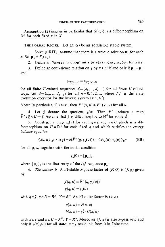
Assumption (2) implies in particular that G(x, .) is a diffeomorphism on RN for each fixed x in X.

THE FORMAL RECIPE. Let (E’, G) be an admissible stable system.

1. Solve (CRIT). Assume that there is a unique solution u, for each x. Set p,=F,(u,).

2. Define an “energy function” on x by e(x) = (JpX, px)[p for x E 1. 3. Define an equivalence relation on x by x z x’ if and only if )L, = p,,

and

for all finite [I-valued sequences d = (d,, . . . . d, ~ i ) for all finite U-valued sequences d = (d,,, . . . . d,- i) for all n = 0, 1,2, . . . . where r,X is the state evolution operator for the inverse system (F”, G’).

Note: In particular, if x z x’, then F” (x, U) z F” (x’, U) for all U.

4. Let jj denote the quotient X/E. Then _ Fx induc_es a map px : j x U -+ 1. Assume that i is diffeomorphic to [Wd for some d.

5. Construct a map y,(u) for each q E 4 and u E U which is a diffeomorphism on U= RN for each fixed q and which satisfies the energy balance equation

(J~,u)~~+e(q)=e(~“(q,y,(u)))+(J~,(u),y,(u)).~

for all q, u, together with the initial condition

Y,(O) = CPJO~

(EB)

where [pL,],, is the first entry of the 12 sequence pq. 6. The answer is: A FI-stable J-phase factor of (F, G) is (f, g) given

by

f(4, u) = Fx (49 Y,(U))

g(q, u) = Y,(U)

with qEj, UEU=R~, Y= RN. An FI-outer factor is (a, b),

a(x, u) = F(x, u)

b(x, u) = rf, 0 G(x, u)

with x E x and u E U = RN, Y = RN. Moreover (f, g) is also J-passive if and only if e(x) 20 for all states XE~ reachable from 0 in finite time.

370 BALL AND HELTON

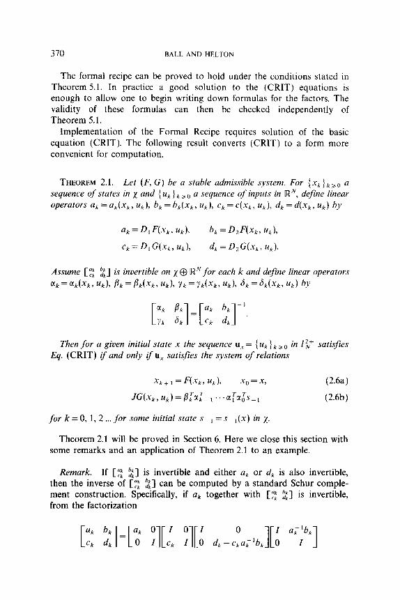
The formal recipe can be proved to hold under the conditions stated in Theorem 5.1. In practice a good solution to the (CRIT) equations is enough to allow one to begin writing down formulas for the factors. The validity of these formulas can then be checked independently of Theorem 5.1.

Implementation of the Formal Recipe requires solution of the basic equation (CRIT). The following result converts (CRIT) to a form more convenient for computation.

THEOREM 2.1. Let (F, G) be a stable admissible system. For {x~}~>” a sequence of states in x and { uk}k 20 a sequence of inputs in RN, define linear operators ak=ak(xk, uk), bk=bk(Xk, uk), ck= c(Xk, uk), dk = d(Xk, uk) by

ak=D,F(XI,, uk)> b, = &F(X,, %),

c,=D,+,, uk), dk = D,G(x,, uk).

Assume [ zi $1 is invertible on x @ RN for each k and define linear operators @k = cLk(xk, uk), flk = Bk(Xk> uk), Yk = Yk(Xk, uk), 6k = hk(Xk, uk) by

Then for a given initial state x the sequence u, = {u~}~>~ in 1 y satisfies Eq. (CRIT) if and only if U, satisfies the system of relations

X k+, =F(xk, uk), x()=x, (2.6a)

JG(Xk,Uk)=p:Cr,T_l...cITcI~S~, (2.6b)

.for k=O, 1, 2 . . . for some initial state s-, ‘s-,(x) in x.

Theorem 2.1 will be proved in Section 6. Here we close this section with some remarks and an application of Theorem 2.1 to an example.

“Ir bk 1s invertible and either ak or dk is also invertible, ,,,“,e~;;,,‘f,,c ;f $k b, ck dJ can be computed by a standard Schur complement construction. Specifically, if ak together with [F; $1 is invertible, from the factorization

INNER-OUTER FACTORIZATION 371

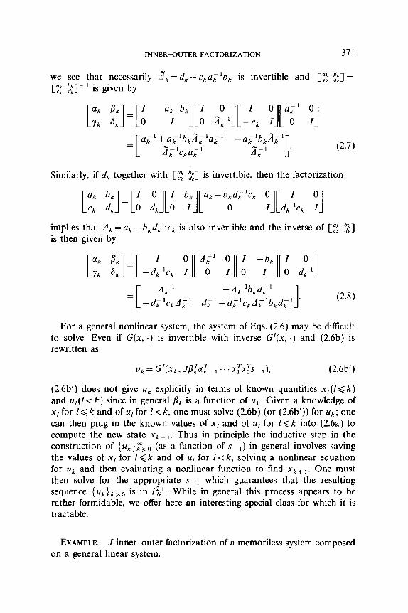
we see that necessarily d, = dk - c,a,‘b, is invertible and [R $1 = C Fi %I-’ is given by

[;: !;I=[:, -a;‘bk][: $I[-‘,, :][“a’ ;I

al’ +aL1bkd”kla-’ k -a;‘b,a,’ = d”; ‘ck a, ’ 1 d”kl

(2.7)

Similarly, if dk together with [:; 21 is invertible, then the factorization

[:; ij=[i :J[:, “;][ak-b~dilck :][d;, ;]

implies that Ak = ak - b,d;‘c, is also invertible and the inverse of [F; 21 is then given by

A,’ -A, ‘b,d;’ = -d;‘ckA;’ 1 d,’ +dklckAklbkdF1 ’ (2.8)

For a general nonlinear system, the system of Eqs. (2.6) may be difficult to solve. Even if G(x, .) is invertible with inverse G’(x, .) and (2.6b) is rewritten as

(2.6b’) does not give uk explicitly in terms of known quantities x,(Z< k) and u,(l< k) Since in general Bk iS a fUnCtiOII of uk. Given a knowledge of x[ for IQ k and of u, for 1 <k, one must solve (2.6b) (or (2.6b’)) for u,; one can then plug in the known values of x, and of U, for I< k into (2.6a) to compute the new state xk+ r. Thus in principle the inductive step in the construction of {z+. } p3 0 (as a function of s ~ 1) in general involves saving the values of x1 for 1 <k and of uI for 1 <k, solving a nonlinear equation for #k and then evaluating a nonlinear function to find xk+ 1. One must then solve for the appropriate sP1 which guarantees that the resulting sequence (~4~)~~~ is in IL+. While in general this process appears to be rather formidable, we offer here an interesting special class for which it is tractable.

EXAMPLE. J-inner-outer factorization of a memoriless system composed on a general linear system.

372 BALL AND HELTON

We consider a system (C) of the form

(Cl .f=Ax+Bu

y = M( cx + Du).

Here the state space x is taken to be R’, the input-output space is taken tobeU=Y=[WN,A:[Wd--,[Wd,B:[WN~(W’,C:iWd~aBN,andD:[WN~[WN are all taken to be linear with D invertible, (A, B) controllable (i.e., span {A’B~ : u E IV, j = 0, 1, 2, . ..} = rWd) and (C, A) observable (i.e., nj,, Ker CA’= (0)), and M: lQN + IR N is taken to be a (possibly nonlinear) diffeomorphism of RN onto itself. The inverse of the linear system

is then given by

(L) T=Ax+Bu y=Cx+Du

(LX) .T=A”x+BD-‘u y= -D-‘Cx+ D-h,

where Ax = A - BD- ‘C. Additional assumptions we impose are

(S) A is stable, i.e., o(A)c D = {z : IzI < l},

and

(D) A x is dichotomous, i.e., A x has no eigenvalues on the unit circle.

Denote by P,“s the Riesz projection for A x associated with the exterior of the unit disk, and denote by A,“, the restriction of A x to its antistable subspace :

A,“,=A” [Imp,“,. (2.9)

We define a nonlinear map W: RN --+ RN by

W(a) = -DM(o)=~JM(o), cJERN (2.10)

and assume

(INV- W) The map W given by (2.10) is a diffeomorphism on RN.

Next, define a map L: Im P,“, + Im P,“, by

L(s)= - f’ (A,“,)- ’ ( +‘)B,,D-’ W-‘((DT)-l B,T,(A,“,r)p’k+l’s), (2.11) ?I=0

INNERCWTER FACTORIZATION 373

where B,,: [WN + Im Pt is given by

B,,=P,“,B (2.12)

and assume in addition that

(INV-L) The map L on Im PC given by (2.11) is a diffeomorphism.

Finally, define an energy function e: Im P,“s + [w by

e(q)= f pJ(Mo Wpl((DT))’ B,‘,(A,“,T))‘““’ L-‘(q))), (2.13) PI=0

where pJ denotes the indefinite quadratic form on RN given by

PAa) = (Jo, o>w.

We then come to the following result.

THEOREM 2.2. Suppose the system Z = (F, G) with

F(x, u) = Ax + Bu

G(x, u) = M( Cx + Du)

is of the form [Memoriless] 0 [Linear] as described above, and assumptions (S), (D), (INV-W) and (INV-L) are all satisfied. Then, for a given XEX=[W“, u,= {ukjkSO is a solution of(CRIT) zfand onZy ~fp, :=F,(u,) is given by

cX= {MO W-‘((DT)-’ BL(A,“,‘)-‘k+“L~‘(PaXsx,,>,,,.

Implementation of the Formal Recipe then leads to a J-inner-outer factorization Z = 0 0 R of Z, where a realization for the J-inner factor 0 is given by

(0) 4=f(q, u)=A,“,q+B,,D-‘M-‘(y,(u))

Y = dq, u) = Y,(U)

with state space equal to Im P,“, while the outer factor R has state space realization given by

Z=a’(x,u)=Ax+Bu

y = bO(x, u) = 7; ,: ~M(Cx+Du) x

with state space equal to P’. Here (q, u) + y&u) (qeIm P,“, and UE WN) is any function from Im P,“, x IWN into [WN satisfying the three conditions:

374 BALL AND HELTON

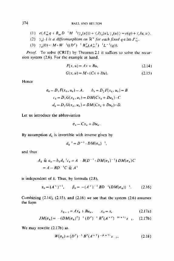
(1) e(A,“,q+B,,D~‘M~‘(~,(u)))+(J;‘,(u),y,(u))=e(q)+(Ju,u). (2) y,( .) is a diffeomorphism on RN for each fixed q E Im Pa:. (3) y,(O) =A40 w-‘((Dq ’ B;;(A,:y’L ‘(4)).

Proof: To solve (CRIT) by Theorem 2.1 it suffices to solve the recursion system (2.6). For the example at hand,

F(x, u) = Ax + Bu, (2.14)

G(x, u) = A40 (Cx + Du). (2.15)

Hence

ak=D,F(xk,uk)=A, b, = D, F(x,, uk) = B

ck = D, G(x,, uk) = DM(Cxk + Du,) 0 C

4 = 4 G(x,, u,)=DM(CX,+DZQ)OD.

Let us introduce the abbreviation

a,=Cx,+Du,.

By assumption dk is invertible with inverse given by

d,‘=D-‘oDM(a,)-‘,

and thus

A, k a,-b,d,‘c,=A-B(D-‘oDM(o,)-‘)DM(o,)C

=A-BD-‘C g A”

is independent of k. Thus, by formula (2.8),

uk=(AX)-l, Bk= -(A”)-‘BD-‘(DM(a,))-‘. (2.16)

Combining (2.14), (2.15), and (2.16) we see that the system (2.6) assumes the form

X k+l=AXk+BUk, x()=x, (2.17a)

JM(o,)= -(DM(o,)~)~’ (DT)-’ B=(A xT)~(k+‘)~~l. (2.17b)

We may rewrite (2.17b) as

W’(CI,)=(D=)-~ BT(A”T)-(k+l’s~,, (2.18)


where W is given by (2.10). Recall that

ck = Cx, + Duk,

where

X k+,=Ax~,+Buk, x()=x.

For Y = bklkao any sequence, let

P(z) = f ZkYk k=O

denote the Fourier transform. Then it is easily seen that

i(z)=(Z-zA)-‘x+z(Z-zA)-‘Bli(z)

and hence

cf(z)=C(Z-zA)-lx+ [D+zC(Z-zA)-‘B] ii(z). (2.19)

Since A is stable and u = u, is required to lie in Ev, we see from (2.19) that necessarily c E I ‘,“. Since A4 is smooth, A4 is Lipschitz on bounded sets and hence the sequence {ZM(flk)}k>O is in Z$+. By (2.17b) this requires that {BT(A”T)~~k+l~~~,}k~o be in I:. If we assume that (A,B) is a controllable pair, then one can show that (BT(A xT)-1, (A” ‘)-‘) is an observable pair, and then { BT(A ’ T)--(k+ ‘) s- i }k30 being in 1 c+ forces that sP1 be in the stable subspace for (A x ‘))‘, i.e., the antistable subspace for A ’ which is Im P,“, .

If we assume that W is invertible (INV- W), we obtain from (2.18) and the above remarks that

CT,= Wp’((D=)-’ B~(A,“,‘)-‘“+“s-~) (2.20)

for some sP1 in Im P,“,. Taking the Fourier transform of (2.20) gives

C(Z-zA)-lx+ [D+zC(Z-zA)-‘B] t;(z)

=n:o Wp’((DT)p’ B,T,(A,“,T)p’“+l’spl)z”.

Thus, if F denotes the transfer function of the system C, that is F(z) = D + z(Z- zA)-‘B, we obtain

F(z)ii(z)= f W-‘((D=)-’ B,T,(A,“,T)-‘“+l’s~l)z”-C(Z-zA)-lx. n=O

376 BALL AND HELTON

The condition that {u,,} E IL+ is the same as tic HZ, in other words, that

f { w-‘((0’) -I B,T,(A,“,‘)-(“+‘)s l)-CA”x} z”EF.l;+. (2.21) n=O

By a direct computation (see [BR3, Theorems 1.2 and 1.33) this condition is equivalent to

Hz0 (A,“,)- (n+l)B,,D-l. { W-‘((DT)-’ B,T,(A,“,7)~‘“+1’s~,)-CA”x} =0

or

-n$o (A,“,)- (,+l)BasD-lW~l((DT)~lB,T,(A,“,T)~(”+l)s~,)=fx, (2.22)

where

r= - f (A,“,)-“+ I) B,,D-‘CA’. j=O

Note that r satisfies the Stein equation

I-- (A,“,)-’ TA = -(A,“,)-’ B,,D-‘C.

From A” =A-BD-‘C we see that

A” -A= -BD-‘C.

Multiplication by P,“, gives

A”P,“,-P,“,A= -P,“,BD-‘C,

so we obtain

P,“,-(A,“,)-‘P,x,A= -(A,“,)-‘B,,D-‘C.

By uniqueness of the solution of the Stein equation (a consequence of the stability of (A,“,)- ’ and A), it follows that r= P,“s . Finally, recalling the definition (2.11) of L(s) and using the assumption (INV-L), we may solve (2.22) for s- , to obtain

s -1 =L-‘(P,“,x). (2.23)

INNERXKJTER FACTORIZATION 377

Note for future reference that L satisfies the nonlinear Stein equation

L- (&yL+i~y= -(A,“,)-’ B,,Dp’Wp’((DT)-’ Ba”,(A,“,T)-l(.)).

(2.24)

Thus

ti,(z)=F(z)-’ [vL-I(p;,)(z)- C(I-zA)-‘xl,

where

Then p,=C,(u,) is given by

pL,= {MO w-‘((DT)-l B,T,(A,“,=)-‘“+“L~‘(P,“,x))}..,.

This completes step 1 of the recipe. Also note that [II,]~ of step 5 is given’ by

[pJo=MO Iv’((DT)-’ B,T,(A,“,T)-’ L-‘(P,“,x)).

We remark that in terms of what follows (in Section 3) this gives the output piece of the desired right pole dynamics for the inner factor. Having solved (CRIT), we are now ready to implement the recipe.

The system inverse to C is

CC-‘) f-(x, y)=(A-BD-‘C)x+lw’MP(y) G’(x, y)= -D-‘Cx+D-‘M-‘(y).

Note L = pxs and IQ; (xl d) = P~;(~~; d) for all n exactly when P,X,x = P,X,x’. The quotient manifold jj = x/w we therefore take to be 2 = Im P; and P,“, as the canonical quotient map. Then

Pyq, y)=A,“,q+B,,D-‘M-‘(y)

&(q, y)= -D-‘Cq+D-‘M-‘(y).

Now it is easily checked that the state space representations for 6I and R

’ We now have the right pole dynamics (y,(O) = [p,lo, f(q, 0) = F” (x, [p,],,) (where q = [xl)) for the desired J-inner factor as in Section 4.

378 BALLANDHELTON

in Theorem 2.1 follow by simply specializing the Formal Recipe to this example.’

The only part of the construction not presented with explicit formulas was the construction of y,(h) satisfying (l), (2), and (3) of Theorem 2.2. That solutions exist is the subject of Theorem 5.1. The proof of this theorem is based on a Morse theoretic lemma, see [BH2, Lemma 3.11 and so construction of y,(u) is in principle as constructive as these lemmas.

A very special case of Example I illustrates what is involved in solving the “energy balance” equations (l), (2), and (3) of Theorem 2.2.

EXAMPLE II. Take the input-output and state space of the system to have dimension one. Also take A=O, B=l, C=l, -l<D<l, and M: R’ + R’, so the system C in Example I is

J-(x, 24) = 24, G(x, u) = M(x - Du).

Then the energy function e is derived via: Set W(q) = M’(q) M(q) and set

V(q)= f D’W’(D’q). /=O

Then (CRIT) is equivalent to V: R + R being an invertible function and the energy function is

e(q) = f [MO Wpl(Dk V’(q))]‘. k=O

Set E,(u, y) = 2.4’ + e(x) - e(F” (4 y)) - Y2,

where

FX(x, y)= -D-‘x-Dp’W’(y).

’ We would like to check that the dynamics CJ,,+ , =f(q,. 0) is stable. The definition off in step 6 combines with previous equations to give

f(q.O)=A,“q++B,,D~‘M-‘(Mn W~‘((DT)-‘B,:(A,“,“)-‘L~‘(q))

=A,“,q+B,,D~‘W-‘((Dr)~‘B,T,(A,:T)L~’(q)).

Note from the Stein equation (2.24),

f(Lq,O)=Lc(A,:r)~‘q.

Thus the dynamics J(., 0) is diffeomorphic to the linear stable dynamics (A,:‘)-’ via the diffeomorphism L-as is to be expected.


We wish to solve E,(u, y,(u)) = 0 for y,(u). Differentiation of this with respect to u leads to

(~w~u)(u~ Y,(U)) yxu)= - (dE,/ay)(u, y,(u))

For each fixed x the substitution A(U) = MP’(y,(u)) leads to the differential equation

dA 224 Z=2W(A)-e’((l/D)[A-x1)(1/o)

with the initial condition on y,(O) yielding

l(O) = w-’ 0 V-‘(x).

Thus solving the energy balance equations for this simple example reduces to solving a first order differential equation with initial condition.

3. BUILDING A SYSTEM WITH PRESCRIBED NULL AND POLE DYNAMICS

In classical complex variables a basic issue is how to build a meromorphic function with prescribed poles and zeros. Important special cases include the case where all poles lie outside the unit disk and are Schwarz reflections of the zeros; this produces inner functions (up to a constant multiple).

The state space versions of such constructions even for matrix valued functions have reached a sophisticated level in recent work of [GKLR, BR3, G, AG, BGRl]. This section extends this approach to nonlinear systems in one sensible way.

a. The General Theorem

The first step is to define nonlinear generalizations of the notion of poles and zeros of (scalar) rational function or null chains of rational matrix functions.

Recall the notation F”, G’ from (2.3) for the system which is inverse to a given system (F, G).

DEFINITION 3.1. Assume that we are given an admissible system (F, G) (see Section 2). Then :

380 BALL AND HELTON

1. The left null dynamics (LND) of (F, G) is F”.

2. The right null dynamics (RND) is the pair of maps C$ ’ : x + x and y x : x --t U defined by

q5 x (x) = F” (x, 0), y x (x) = G’(x, 0).

3. The left pole dynamics (LPD) of (F, G) is F.

4. The right pole dynamics (RPD) is the pair of maps 4: x + x and y:x+ Ydetined by

4(x)= FC’(x, OL Y(X) = G(x, 0).

The reader should observe that LPD (resp. RPD) for (F, G) equals the LND (resp. RND) for (I;“, G’).

A system (F, G) as in (3.1) is said to realize the mapping W: 1; -+ Zz if W is the IO map F0 for (F, G) with 0 initial condition. The problem of constructing (F, G) from the IO map W is the realization problem in systems theory. If W is causal then the well-known Nerode construction (see [K]) can be seen to yield a formal realization for a given IO map W, with additional smoothness and nondegeneracy assumptions one can arrange that even (F, G) is an admissible system (see [S, J] for continuous time versions). The goal of this section is to obtain realizations for a system from types of information different from a knowledge of the whole IO map.

We next define notions of null and pole pairs for an IO map in such a way as to guarantee independence of these notions from any particular admissible realization of the IO map.

DEFINITION 3.2. Let W be a causal mapping on I$+ having at least one admissible realization. Then

1. The mapping Fx is a left null dynamics LND for W if F x is the LND for some admissible realization of W.

2. The pair of maps (4 x, y x ) is a right null dynamics for W if ($ x, y x ) is the RND for some admissible realization (F, G) of W.

3. The mapping F is a right pole dynamics for W if F is the RPD for some admissible realization (F, G) of W.

4. The pair of mappings (4, y) is a right pole dynamics RPD for W if (4, y) is the RPD for some admissible realization (F, G) of W.

We say that two nonlinear systems (F, G) and (p, G) are similar if there

INNERXHJTER FACTORIZATION 381

is a state space diffeomorphism S: I+ x preserving the equilibrium points for which

F(x, u) = s-‘F(S(x), u) (3.1)

G(x, u) = G(S(x), u). (3.2)

In this case, pq = Fscq,, so the two systems (F, G) and (F, G) generate the same set of IO maps and & = &. Thus if F” is the LND for an IO map W and Fx : 2 x U + i is similar to F” in the sense that

Fx (x, u) = S-’ 0 F” (S(x)) (3.3)

for a diffeomorphism S: 2 -+ 1 mapping 0 to 0, then px is also a LND for W. Similarly, if (4, y) is a RPD for W and (& 7) is similar to (4, y) in the sense that

&x) = s- V(S(x)h y”(x) = Y(e)) (3.4)

for a diffeomorphism S, then (4, 7) is also a RPD for W. Similar statements obviously hold for RND and LND. In the linear case with observability and controllability assumptions, there are also converses to all these state- ment (e.g., any two LNDs for the same IO map W are similar), but in the nonlinear case these issues are more complicated (see [I]).

A key problem for us is building an IO map W or an admissible system (F, G) with prescribed LND and RPD. Related problems of course include building W or (F, G) from LND and LPD, or what compatibility conditions on LPD, RPD, LND, and RND guarantee there exist a corrsponding system (see [GKvS] for the linear case). Here we shall concentrate on the first problem.

Related notions of zero dynamics have recently been introduced and studied by several authors (see [IM] for a survey). It remains for further work to see how our notions are related to these.

The following is a nonlinear version of at least one direction of one of the main results of [GKLR].

THEOREM 3.1. Suppose we are given smooth maps

F”lXXlJ-+X

41X-+X

y:x+u.

Then there exists an input-output map W with admissible realization (f, g)

5801104%IO

382 BALL AND HELTON

having F” as a LND and (4, y) as a RPD if there exists a diffeomorphism S of x which satisfies the nonlinear Sylvester equation

Sodb) = F” (S(x), Y(X)). (3.5)

For any such S an appropriate choice of (f, g) is any admissible system ,for which

f(x, u)= F” (x, Ax, ~1) (3.6)

g(4 0) = y(S- ‘(x)). (3.7)

Note that essentially the only restriction on g in Theorem 3.1 is its value at points of the form (x, 0) and that g(x, .) be a diffeomorphism on lRN for each fixed XE x. Thus in the nonlinear context there can be many inter- polants associated with the same solution S of the Sylvester eqaution (3.5), contrary to the situation for the linear case [GKLR, BR3].

The role of this theorem in the recipe in Section 2 will be made clear later. The main link is that to perform an inner-outer factorization (F, G) the LND information is obtained immediately as Fx , while the solution to (CRIT) can be used to produce RPD information. In Section 4 we apply a theorem like Theorem 3.1 to obtain an inner system having the given functions as LND and RPD.

Proof of Theorem 3.1. Let (f, g) be given as in the recipe. The inverse system (f x, g ’ ) by definition is the pair of maps such that the system of equations

1=f”(x, Y)

u=g”b, Y)

is equivalent to the system

Z=f(x,~)=F~(x,g(x,u))

y = g(x, u).

Thus, solving the second equation for u in terms of y gives

g ” (x9 Y) = g’k Y).

Substituting this into the first equation gives

f x (x, VI = F” (x, g(x, g’k ~1) = F” (x, Y)

INNERCKJTER FACTORIZATION 383

and hence f x = F” as wanted. Next note that

f(x,O)=F"(x, g(x,O))=F"(x,y(S-'x))

dx, 0) = YWYX)).

Replacing x with S(x) yields the identities

f(S(x),O)=F"(S(x),y(x))=S(~(x))

‘!dS(X)> 0) = Y(X).

Thus

s-'~f(sx,o)=qqx)

g(Sx, 0) = Y(X).

Thus (4, y) is the RPD for the admissible system (x g) defined by

i34 u) = ‘!dS(x), u).

Thus (x g) is similar to (f, g), so (1 2) is also an admissible realization of W. This establishes that (4, y) is a RPD for W. 1

The converse to Theorem 3.1 (namely, the question as to whether every LND and RPD for an IO map arises via the construction in the theorem) is problematical since we do not know that LND and RPD for the same IO map are similar. One can obtain a converse direction by formulating the interpolation problem as that of constructing a system (F, G) with given LND F” and with RPD similar to a given pair (4, y ).

b. The Sylvester Equation

Clearly the key to Theorem 3.1 is a solution of the nonlinear Sylvester equation (3.1). Under some stability assumptions, the problem of finding a solution turns out to be tractable; one has a unique solution together with a representation for the solution.

To localize our nonlinear notions of null and pole dynamics, we need some idea of a “stable” sequence. Recall that we denote by l’,” the space of sequences in Z$ which are square summable in norm. The l? norm is convenient as a measure of energy but other notions of decay at infinity might also be used. Recall from Section 2 that a system (F, G) is said to be stableifuEl$+::y=&(u)EZ~+; a dynamics F by itself is said to be stable if the system (F, I) is stable, where Z is the state readout map

384 BALL AND HELTON

To describe the solution we need some notation. Given an admissible system (F, G) let F, denote the inverse of F for fixed u (it it exists), namely

F,(F(x; u), u) =x, F(F,(x, u), u) = .Y.

We call F reversible if such an F, exists and we call F1 the reverse dynamics. Recall the notation P, in (2.7) for the state evolution map associated with a dynamics F. We write [r; 1, to denote the state evolution map associated with the reverse dynamics [F”], associated with the inverse system.

THEOREM 3.2. Suppose F x, 4, and y are as in Theorem 3.1. Suppose in addition that

Define for each x E x and n = 0, 1, 2 . . . an element x,(x) E x by

x,(x) = [r; 1, (0; yap”(x), yoqw2)(x), . ..) y(x)). (3.8)

Then if

x,(x)= lim x,(x) n+m

(3.8a)

exists for each x E x, then the solution S of the nonlinear Sylvester equation (3.5) is unique and is given by

S(x) =-&Ax), x E x.

An alternative form for the unique solution of (3.5) is the following; this formula has the advantage that it avoids reference to backwards time.

PROPOSITION 3.3. Suppose F”, 4, and y are as in Theorem 3.2. Then the unique solution x + S(x) of the nonlinear Sylvester equation (3.5) is determined by

lim [TX 1, (S(x); y(x), y 0 f+(x), . . . . y 0 d(“- l)(x)) = 0. n-m

Proof of Theorem 3.2. Since [F” 1, is stable and (y o~(“)(x))~=~E I$+ for each x E x by assumption, it follows from the stability of [F” 1, that (x,(x)) defined by (3.8) is convergent to an element x,(x) of x.

To see that x,(x) is a solution of the Sylvester equation (3.5) whenever the limit (3.8a) exists, note first that (3.5) can be rewritten as

CF” I, (SOL> Y(X)) = S(x). (3.9)

INNERCIUTER FACTORIZATION 385

By induction one can show that

x,, I(X) = [F” II kl~d4X)Y Y(X)) (3.10)

with x0(x) = 0. Taking limits in (3.10) and using continuity of [F” 1, then gives that S(x) =x,(x) is a solution of (3.9), and hence also of (3.5).

Conversely, suppose x + S(x) is a solution of (3.5), or equivalently of (3.9). By iteration we obtain

S(x) = CF” I, (Sod(x), Y(X))

= CF” 1, (L-F” II (~~#‘YX)~ Y”&X)), Y(X)) = CC12 (ASP’; YOdb), Y(X)).

By induction one can show in general that

S(x)= Cr; 1, (x”d’“‘(x); y4(n-1)(x), . . . . Y(X)) =.“1”, [r;], (SO@“)(X); YO&~-~)(X), . . . . y(x)). (3.11)

Note by hypothesis d’“‘(x) tends to the equilibrium point 0 and from (3.9) we see that S(0) is also an equilibrium for [IF” II, so by uniqueness of the equilibrium point S(0) = 0. Then by uniform continuity of [F” I,, we conclude from (3.1) that

S(x) = lim [f? I, + , (0, y 0 d’“‘(x), . . . . y(x)) n-rm

=x,(x).

Thus x,(x) is the unique solution. 1

We remark that the condition that the limit (3.8a) defining x,(x) exist can be interpreted as a stability requirement on the reverse dynamics CF” I,, or equivalently, as an antistability requirement on the forward dynamics F x. Indeed, in the linear case where F(x, u) = A ‘x + Bu, the existence of the limit (3.8a) for all x E 1 is equivalent to the matrix A x having all its eigenvalues inside the unit disk.

Proof of Proposition 3.3, Suppose 2, E x is such that lim, _ m Z-,(x) = 0, where

%l(x) = rrx 1, bfm; Y(X), y o d(x), . ..1 y o 4’“- “(4).

This quantity represents the state at time n if the initial state at time 0 is Z,(x) and the string of inputs y(x), . . . . yod(“-l)(x) is fed into the forward dynamics F” (x, u). Equivalently, we recover Z,(x) by initializing at f, and

1,

386 BALL AND HELTON

then feeding y 0 4”’ ’ ) (x), . . . . 7 J d(x), y(x) into the reverse dynamics [F’ thus

Z.,(x) = [ry 1, (a,,(x); y c qP- ‘j(x), . ..) y @$b(X), y(x))

=& tIr; I,, (2,(-x); y o P “(XI, .‘.> Y o b(x), ‘l(x)).

Again by continuity of [F” I1 and since lim,, r* Z,(x) =0 we obtain

g.,(x) = !imz If; 1, (4; Y~JP”(x), . . . . Y(X)),

=x,(x),

where x,(x) is as in Theorem 3.2. Conversely, suppose x,(x) is defined as in Proposition 3.3, namely,

x,(x) = lim x,(x), where

x,(x) = [f?], (0; y 0 qv- “(X), . ..) y(x)). Expressing this relation in terms of the forward dynamics F" rather than the reverse dynamics [F x 1, gives

[fX 1, (x,(x); Y(X), 7” d(x), .‘., Y o d’“- “(X)) = 0.

Taking limits and using continuity of F" then gives

lim [fx 1, (x,(x); y(x), . . . . y 0 f$‘“- ‘j(x)) = 0 “-+CS

and then x,(x) = j?.,(x) is as in Proposition 3.3. m

The S required by Theorem 3.1 is a diffeomorphism while the S produced by Theorem 3.2 need not be invertible. At this level of generality little is known about what conditions on I;", 4, y imply invertibility even in the linear case (see [DD]).

4. LOSSLESS SYSTEMS FROM GIVEN LND AND RND INFORMATION

Our main interest for applications to control theory is the construction of input-output maps preserving some Hermitian form on ZF (see [BH2] ). Let J= JT = J- ’ be some fixed real N x N symmetry matrix and let pJ: I$+ -+ [w be the associated quadratic form


on li+;‘, or pJ(u)= (Ju, U)~N on RN; in the context of the scattering formalism in circuit theory, pJ measures the energy of an input or output signal (see [AV] ). We are interested in IO maps W on Zp which are energy-conserving (with respect to J), i.e., maps W for which

PJ” w(u) = PJt”)

for all u E I’,‘. One way of constructing energy preserving IO maps is to realize them as the IO map of an energy-conserving system (see [AV]). Let e be some energy function e: x + 174 defined on the state space x. We say that a system (f, g) is e-conseruing if there is some energy function e: x + R on the state manifold 1 for which

PJc”) + e(x)=pJk(x? u)) + e(f(xy u)) (4.1)

for all x in x and inputs u E U. We shall usually assume that at least e is continuous and that e(0) = 0, i.e., that the equilibrium state has 0 energy. A system is said to be lossless if it is e-conserving for some e. The following result gives the connection between e-conserving systems and FI-stable J-phase (and possibly also J-passive) IO maps.

THEOREM 4.1. Suppose that (f, g) is an e-conserving admissible system (with respect to J) for some continuous energy function e: I-+ R on the state space x. Suppose in addition that

(1) For each initial state q reachable from the equilibrium state 0 in a finite time, if y = ( Y,,}“>~ is defined by

X ntl =f(xm Oh x0=9

Yn = &L, 0)

then C,“= o II y, I( 2 < 00 and lim, _ o3 e(x,) = 0 and

(2) the equilibrium state 0 has zero energy

e(0) = 0.

Then the IO map 0 = f. associated with (f, g) and O-initial state is FI-stable J-phase. Moreover, if e(q) B 0 for all q E x, then 8 is J-passive as well (so 0 is J-inner).

Proof Let u(u,, . . . . u,, 0, 0, . ..) be a sequence in Ify’ having finite support. Then y = e(u) is given by

xn+ 1 =fbn, 4x), x,=0

Yn = g(x,, %I).

388 BALL AND HELToN

Application of (4.1) gives in general that

Summing from 0 to K and using that e(xO) = 0 gives

4xK+ I) = ; P”f(kr- f PJ(Yk). k=O k=O

(4.2)

Since uk = 0 once k > N, the stability assumption (1) implies that Y= CYA2OG+)N+, and hence 0 is FIstable. Moreover, since by (1) we also have lim, _ 5. e(x,) = 0, taking limits in (4.2) shows that p,(o(u)) = pJ(u), so 0 is a J-phase map. If e(q) 2 0 for all q, then it follows immediately also from (4.2) that 0 is J-passive as well. 1

It is possible to formulate and prove a converse to Theorem 4.1, namely, one can show that any FI-stable J-phase (and J-passive) IO map 6’ has a lossless realization as in Theorem 4.1. As we shall not need this result we shall not pursue this point here.

For the sake of future applications we shall consider in the following theorem the construction of lossless systems which need not be stable (i.e., the state dynamics need not be FI-stable as was assumed in Theorem 4.1). The result is as follows:

THEOREM 4.2. Suppose N = 2 or J= I and that F” and (rp, y) are smooth maps with F”:xx Y-,x, cp:x+x, y:x-+ Y. Then F” is the LND and (cp, y) is the RPD for some admissible lossless system (f, g) if:

( 1) The compatibility condition

cp(x) = FX(x, Y(X))

holds,

(2) There is a continuous energy function e: x -+ IF8 with e(0) = 0 such that for all x E x the function

satisfies

a.&)= (JY, Y)w+~(P~(~, Y))-e(x)

(CRIT) a, has exactly one critical point which is equal to y(x).

(co CRIT) a, has no critical point at infinity in the sense that 11 Va,( y)ll > 6 > 0 for all y in the complement of a bounded neighborhood of Y(X).

(HESS) The Hessian [Hess a,][y(x)] of a, at its unique critical point y(x) has the same signature as J.


In this case, the recipe for the system (ft g) is

f(x, u)= F” (x, g(x, u)),

with g any smooth function for which

(i) g(x, .) is a dlffeomorphism of RN for each x,

(ii) a,(g(x, a)) = (Ju, u)N for all x and a, and

(iii) g(x, 0) = y(x).

Conversely, if there exists an admissible lossless system (f, g) having F” as LND and (f, g) as RPD, then necessarily (1) holds, and the function y + a,(y) for each x E x determined by a suitable energy function e satisfies (CRIT) and (HESS).

The hypothesis N = 2 or J= Z is needed only to guarantee that a key lemma from [BH2] is applicable. This is only for technical convenience; we expect that this hypothesis is not necessary for the lemma, and hence also not necessary for the validity of Theorem 4.2. The converse direction in Theorem 4.1 holds without the hypothesis that N = 2 or J= I.

Proof Suppose (f, g) is a lossless system (with energy function e on the state space) for which F” is the LND and (cp, y) is the RPD. Then necessarily

and

v(x) =f(-T O), Y(X) = g(x, Oh (4.3)

F” (x, dx, u)) =f(x, u). (4.4)

Specializing (4.4) to u =0 and combining with (4.3) then gives the compatibility condition (1) in Theorem 4.2. By definition of (F, G) being e-conservative with respect to J, we have

e(x) + <-k u>N=e(f(x7 u)) + <Jg(x7 u), dx? u))N. (4.5)

Rewrite (4.5) as

axk(xT u))= (h u)N. (4.6)

Since g(x, .) is assumed to be a diffeomorphism of Y = RN for each x E x, by [BH2, Lemma 3.91, (4.6) forces the critical point structure of y -+ a,(y) to be the same as that of u+ (Ju, u)~. By the analysis there we see that y(x) = g(x, 0) must be the unique critical point of a, so (CRIT) holds. Moreover the Hessian of a, at its unique critical point must have the same signature as the Hessian of u + (Ju, u) at u = 0, namely, the same

390 BALL AND HELTON

signature as J, so (HESS) holds. This proves the necessity direction in Theorem 4.1.

Conversely, suppose conditions (1) and (2) in Theorem 4.2 hold. Then by [BH2, Lemma 3.93 there exists a smooth function g(x, U) such that

(i) g(x, .) is a diffeomorphism of Y for each x E x, (ii) g(x, 0) = y(x), and (iii) the identity (4.6) holds.

We then define f(x, u) by

Ax, u) = F” lx, Ax, ~1).

That the system (f, g) is J-lossless with respect to the energy function e is a simple consequence of the identity (4.6).

We next check that (f, g) is an admissible system. Smoothness of g is guaranteed from the construction from [BH2, Lemma 3.93; then f is also smooth on the composition of smooth maps. Since by construction g(x, .) is a diffeomorphism for each fixed x, the inverse function g’ such that

g(x* AX> Y)) = Y

g’(x, g(4 u)) = u

exists and is smooth. As f” (x, y), the system (f”, g’) inverse to (f, g) exists and is smooth. 1

Remark 4.3. If in Theorem 4.2, one wants to build a J-lossless system (f, g) for which in addition to the other requirements, the state dynamics f is FI-stable in the sense of Theorem 4.1, then necessarily, since f(x, 0) = q(x), one must have

(4.7)

for each state x E x. Conversely, if (4.7) holds together with all the assumptions of Theorem 4.2, then one can build as in Theorem 4.2 an admissible J-lossless system (f, g) for which the state dynamics f is FI-stable. Then by Theorem 4.1 the associated IO map 8 =fO is a FI-stable J-phase. Since y is smooth and y(O) = 0, then from (4.7) we also have

(4.8)

for each x E x, This stability assumption enables us to solve (4.5) (with u set


equal to 0) uniquely for the energy function e. Indeed, from f(x, 0) = q(x) and g(x, O)=y(x), (4.5) with u=O gives

e(x)= e(cp(x)) + (JY(x), Y(X)>. (4.9)

This equation can be interpreted to be a nonlinear Stein equation for the function e. Iteration of this gives

4x) = e(cp’*‘(x)) + (Jr 0 rp(x), y. dx) > + (JY(x), y(x)) n-l

= e(cp(“)(x)) + C (Jy 0 cp(j)(x), y 0 cpcJ)(x)). (4.10) j=O

By our stability assumption, lim,, m cp’“‘(x) = 0 and e(0) = 0. Thus (4.9) implies that an energy function e is necessarily given by

e(x) = 5 (Jy 0 q(j)(x), y 0 q(j)(x)). j=O

(4.11)

Conversely, the condition (4.8) guarantees that the expression (4.11) for e is well defined and one can then verify by direct substitution into (4.9) that it defines a solution of (4.9). We conclude that the energy function e required in Theorem 4.2 is uniquely determined by the other data of the problem in the case where cp is stable in the sense of (4.7).

Theorem 4.2 is a crude first theorem on the general problem of constructing a lossless system from given LND and RPD, but it is adequate for our application in the next section. Variations which would also be of interest to sovle are:

1. Given F” , (cp, y ) and e, find an e-conserving system (f, g) which has LND and RPD similar to F” and (cp, y), respectively.

2. Given F” and (cp, y ), find a J-phase IO map W which has F” as a LND and (cp, y) as a RPD.

3. Given F” find an energy function e and an e-conserving system (J g) which has LND equal to (or similar to) F” .

4. Given F” find a J-phase IO map W which has F” as a LND.

The first question can be treated by the likes of Theorem 4.1; the answer to the first question (once one finds an appropriate energy function e) then gives sufficient conditions under which one can answer the second question. The third question is harder and actually closer to inner-outer factorization itself. The relation of the fourth question to the third is just like that between the second and the first.

In the linear cased the LND determines a RPD (up to similarity) via

392 BALL AND HELTON

Schwarz reflection; in the nonlinear case this is not available. In section 5 we will show how to obtain RPD from LND in the context of inner-outer factorization where some additional information is present.

We offer the following simple results concerning the first and third questions.

THEOREM 4.3. Suppose N = 2 or J= I. Suppose F” and (cp, y) are as in Theorem 4.1 and that they meet the stability hypotheses of Theorem 3.2, and let an energy function e on x given be given. Then there is an e-conserving admissible system (f g) with LND equal to F” and RPD similar to (cp, y) if:

(1) there is a diffeomorphism S on x which satisfies the nonlinear Sylvester equation

Socp(x) = F” (S(x), Y(X)), XEX (4.9’)

and

(2) for each x E x the function a, defined by

a,(v) = (JY, Y )N + 4F” (x9 ~1) -4x) (4.10’)

satisfies

(i) a, has exactly one critical point which is equal to y(S’(x)),

(ii) for each neighborhood U of y(S l(x)) there is a 6 > 0 for which IIVa,X( y)Ij 2 6 if y is in the complement of U,

(iii) the Hessien of a, at y(S ‘(x)) has the same signature as J,

(iv) a,(y(S’(x))) = 0 for all XE x.

Conversely for an e-conserving admissible system (f, g) having LND equal to F” and RPD similar to (cp, y) to exist, it is necessary that there exists a diffeomorphism S of x satisfying (4.9), and that the function a, defined by (4.10) satisfy (i), (iii), and (iv).

THEOREM 4.4. Given F” to build a lossless (f, g) with F” as a null pair it is sufficient to find (cp, y ) and e, S satisfying the conditions (1) and (2) of Theorem 4.3.

The proofs of Theorems 4.3 and 4.4 are routine exercises of putting together the ideas in the proofs of Theorems 3.1 and 4.1, and so will be omitted.


5. INNER-OUTER FACTORIZATION: PROOFS

In this section we construct a FI-stable J-lossless factor (f, g) for a given stable system (F, G), that is we verify the validity of the formal recipe of Section 2. The strategy is simple in light of Section 4. First, we show that F” is a LND for the desired (f, g). Then we show that the solution of (CRIT) gives a stable RPD for (h g). Thus Theorems 4.1 and 4.2 construct (f, g). It is in this manner that we prove the main theorem of the paper.

In the nonlinear case the J-phase factor (f, g) in a J-phase-outer factorization (F, G) = (f, g) 0 (a, b) is highly nonunique; in particular it is possible for the state space of the J-phase factor to be arbitrarily large. However, we shall show that under certain conditions on (F, G) the state space i for (f, g) as well as for (a, 6) can be taken to be a quotient space of the state space 1 for (F, G), as is the situation in the linear case. If we do not insist on some sort of controllability and observability we may assume that the state space for (a, b) (and its inverse (ax, b’)) is equal to the state space x for (F, G). Then (f, g) = (F, G) 0 (ax, b’) formally has state space xxx but the states reachable from 0 may be submanifold of x x x. We now formalize the notion of a standard J-phase-outer factorization.

DEFINITION 5.1. Let (f, g) and (a, b) be stable admissible systems for which (f, g) is FI-stable J-lossless and (a, b) is FI-outer. Then the factorization (F, G) = (f, g) 0 (a, b) is said to be a standard J-phase-outer factorization if (F, G) and (a, b) have identical state spaces x and the set of states in x xx reachable from 0 x 0 for the composite system (F, G)o (a x, b’) consists of the submanifold {(x, x): x E x}.

Recall from Section 2 the Formal Recipe for constructing J-phase-outer factorizations.

THEOREM 5.1. Given an admissible stable system (F, G) the Formal Recipe produces an admissible standard FI-stable J-phase-outer factorization

(F, (-3 = (f, 810 (a, b)

provided that:

(CRIT) For all XEX, LWx(u) [J9?x(u)] = 0 has a unique solution u, E 1 i+. Set p, = Px(u,)

(PROP CRIT) The correspondence x -+ c, is proper, i.e., the set {x E x: p, E X} is precompact in x whenever 2” is a compact subset of l’,W, co).

394 BALL AND HELTON

(co CRIT) For each x E 1 there exists an integer p < z so that ,fi)r each neighborhood U of P,,u, = ([a,],,, . . . . [u,]~) E l,[O, p] there is a 6 > 0 for which

if P,u = (u,, u,, . . . . up) is not in U.

(HESS) The bilinear form

(h, k) + (JDFx’,(u)Chl, DFx(u)Ckl> + <JFx(u), D2F.x(uP, kl>

is nondegenerate on 12 x 1: for u = u,, for each x in x.

(Q) The quotient manifold jj defined in the Formal Recipe is diffeomorphic to [W’.

(co G) The derivative D,G(x, u) of G with respect to the input variable u is uniformly bounded above and below on [WN, i.e., for each x E x there exist positive numbers m, and M, such that

for all hE [WN.

m, llhll G lI&Gb, u)Chlll d K llhll

In this case (f, g) can be constructed to have FX as its LND and (4, y”) as its RPD, where

px (4, Y) = CF” lx, ~11, (5.1)

4(q) = CF” (x, C~,lo)l> (5.2)

and

7(q) = CL10 (5.3)

if q = [x] is the equivalence class containing x. Moreover the system (f, g) is J-passive if (Jp,, cl,) 2 0 for each x E x.

Conversely, if (F, G) has an admissible standard stable J-phase-outer factorization

(F, G) = (f, g)o (a, 6)

then necessarily (CRIT) and (HESS) holdfor (F, G), the state manifold 2 for (f, g) can be identified as the quotient space i = ~1% of x with respect to some equivalent relation z on x, and the maps Rx, (4, 7) defined by (5.1)-(5.3) with respect to the equivalence relation x are the LND and RPD respectively for (f, g).


Remark 5.1. The assumption (Q) that i is a smooth manifold diffeomorphic to IWa looks rather presumptions but in fact is reasonably well justified. Indeed, if cp: x + x is defined by

v(x) = F” (A Y,(O))

and if the correspondence x + p, is injective, then it can be shown that cpr”](x) tends to 0 for each x E x. Moreover, as we shall see later cp induces a well-defined map @ on 2 and +( [xl) -+ 0 as n -+ co. If we assume that the original system (F, G) is the discretization of a continuous time system with a small time step size, then iterates of ~JJ move points very little compared to the scaling of the manifold, and a precise theorem well-known among topologists implies that 2 diffeomorphic to IF!? We thank our colleagues M. Friedman and F. Quinn for illuminating discussions concerning this point. 1

Remark 5.2. In addition to the distinction between FI-stable vs stable factors and the technical conditions (PROP CRIT), (cc ), and (00 G), the gap between the necessary and sufficient sides in Theorem 5.1 has to do with the size of the state manifold. Assumption (Q) guarantees that the state manifold can be taken to be a minimal size, but in general a standard J-phase-outer factorization conceivably may exist without its state manifold being diffeomorphic to [Wa or perhaps with its state manifold equal to a larger quotient space of x.

Proof of Theorem 5.1. We first argue the necessity of the conditions (CRIT) and (HESS). Thus suppose the stable admissible system (F, G) has a factorization (F, G) = (f, g) 0 (a, b) with (f, g) an admissible stable energy-conserving J-phase system and with (a, 6) an admissible outer system. Then the system (a x, b’) inverse to (a, b) is also outer and

(f’, G)o(a”,b’)=(f, 8). (5.4)

This implies the factorization of IO maps (with initial state set equal to 0)

Foe [ax lo=fo. (5.5)

Denote by pJ the quadratic form

PAY) = (JYV Y>.

Here we abuse notation and consider pJ as acting on [WN, I’,” or I, [0, n]; the meaning will be clear from the context. Now the IO map f. for the J-phase system satisfies pJo fO = pJ, hence (5.5) implies

(5.6)

396 BALL AND HELTON

Since (a X, h’) is an outer admissible system, [a X lo is a diffeomorphism of Ii? onto itself. Moreover, the compression P,,[a” I,, 1 /,w[O, n] is a diffeomorphism of I,[O, n] onto itself for each n = 0, 1, 2,

Now let x be an arbitrary state in the state space x for the system (F, G). We need consider only states XE x which can be reached from the equilibrium state 0 by feeding in finitely many inputs i?,,, . . . . u”,, i.e., there exists ? E 1; [0, n] for which

As was observed above, there exist a v E 1; [0, n] for which

i=P,[a”],(v,O).

Now if u = (u,, ui, u2, . ..) is any sequence in I$+ we may juxtapose it next to uEINIO,n] to form a sequence (v,u) in 12:

(v, u) = (u,, . . . . u,, uo, Ulr u2> . ..I.

If ?;,,I is the state evolution map associated with ax

C+1(4, a=4 if 9 = x,+ , where 5 = (to, . . . . r,),

tj+l=""(XjT iJ,)> x0=4,

and we set ,? = r,, + ,(O, v), then

[ax lo (v, u) = (f, u) = K Ca x 11 (u))

and

Foe Ca x lo (~7 u) = (v’, F.xo [ax I.: (~11, (5.7)

where

Since we are assuming that the factorization (F, G) = (i g) 0 (a, b) is standard, we may take 2=xX. In general for y= ((y,, y,, . ..)EZ$+. pJ(y) is given as the sum

PJ(Y)= f CJYj3 Yj>UP. j=O

Thus (5.7) gives

~~~Fo~C~“lo(v,u)=~,(v’)+~,~~~~C~”l,(u)


and we also have P.&i u) = PJ(V) + PAU).

The identity (5.6) applied to the element (0, U) E 1:’ therefore becomes

PJ(V’) + ~.roFxo ILax Ii (u) = P,(V) + PJ(U). (5.8)

In all this analysis we consider the initial input string v E I, [0, n] as fixed and u~I2 as variable; note that v’, x are functions only of v and are independent of the choice of u. Define a function H,: If,,? + R by

H,(u) = PAv’) + ~,oFx(u) - PAv). (5.9)

Then (5.8) can be written as

ff,~C~“l.=~,. (5.10)

Since (a x, b’) is outer, we also have that [a x 1, is a smooth diffeomorphism of 12 onto itself. Thus H, and pJ are congruent in the sense that one can go from one to the other by a diffeomorphic change of variable. This implies that H, and pJ must have the same critical point structure on lc+, i.e., there must exist a one-to-one correspondence between critical points of H, and pJ and the critical values and signatures of the Hessians at corresponding points must be the same; this is stated in [BH2, Lemma 1.31 for the case of RN in place of 12, but the proof of this (easy) necessity direction holds for general (even infinite dimensional) manifolds.

The critical point structure of pJ is easily computed. The unique critical point is 0 and the Hessian at 0 is the nondegenerate bilinear form (u, v) + (Ju, v ),c . Thus the map H, defined by (5.9) must have a unique critical point u = u, and the Hessian of H, at u, is nondegenerate. Since the IO map YX depends only on the initial state x and not on the sequence v of initial inputs chosen to reach x, it is clear from the form (5.9) of H, that the critical point u, in fact is uniquely determined by the state x, and hence may be denoted as II,.

From the chain rule

DH,(u)Chl = 2(JF,(u), W(WOh;+

and hence the gradient of H, is given by

VH,(u) = 2 DF,(u)~ [JF,(u)]

and the Hessian of H, is given by

~2H,(u)Ch kl = 2<JDFx(u)Chl, DFx(u)Ckl> + 2(JFx(u), D2Fx’,(u)Ch, kl>.

This completes the proof of necessity of (CRIT) and (HESS).

580/10‘~2-I I

398 BALL AND HELTON

Since we are assuming that the factorization (F, G) = (f; g)a (a, 6) is standard, the state space for the composite system (A g) = (F, G) 0 (ax, h’) can be taken to be the submanifold ((x, x): x E x > of 1 x x which in turn can be identified simply with x via (x, x) --t x. The true state space f for (f, g) can therefore be identified as a quotient space i =x/ x with respect to some equivalence relation z on x.

By a further analysis of (5.8) we can show that necessarily px defined by (5.1) is a LND and ($,I) defined by (5.2) and (5.3) is a RPD for (f, g), where (5.1 t(5.3) are defined using the equivalence relation Z. Indeed, as was remarked above but has not yet been used, the change of variable diffeomorphism [ax 1, in (5.10) or (5.8) must map the unique critical point 0 of pJ to the unique critical point u, of H,., i.e.,

Ca x 1.x (0) = 5.

Thus the critical value Rx = ~Ju,) satisfies

9i” Ca x Ix (0) = Px. (5.11)

But since

V’, G)o(a”, b’)= (f, g), (5.12)

and we are dealing with a standard factorization, (5.12) implies the factorization of IO maps

F.xo [ax l.x=fcxp (5.13)

where [x] is the x equivalence class containing x. Then by (5.11) we have

f[.x,(O) = P.X. (5.14)

In particular, we read off from (5.14) the output at time 0 if the initial state is [x] to be

gtCxl,o)= cPxlo=~(cxl)~ (5.15)

By definition, if the system (F, G) is in the state x at some initial time and the output [Rx& is observed at that same point in time, then the new state .Z is given by

2 = F” (x, C~xlo).

Combining this with (5.11), (5.13), and (5.14) gives

f(Cxl, 0) = [F”k Ccr,lo)l= @([1x1). (5.16)

INNERXWTER FACTORIZATION 399

Conditions (5.15) and (5.16) now imply that (4, 7) is the RPD for (f, g). Again from (5.13) and the definition of I;“, we see that if (f, g) is in state [x] and produces output y, then the new state must be [a], where 2 = F” (x, y); thus

f” ([xl> Y) = CF” CT Y)I = px ([xl, Y). (5.15)

From (5.16) we see that px is the LND for (f, g) as asserted. This completes the proof of necessity in Theorem 5.1.

Now suppose that the stable admissible system (F, G) satisfies (CRIT) and (co CRIT), (HESS), and (Q); we wish to prove that the Formal Recipe produces an at least FI-stable J-phase-outer factorization. Steps 1-4 of the Formal Recipe are well defined. In addition, to the state operator F x :x x Y + x for the inverse (F” , G’) of (F, G), define maps cp: x + x and y:x-+ Y by

and

dx) = F” (x> Clrxld (5.18a)

(5.18b)

The equivalence relation - defined in Step 4 one easily verifies is such that

X%X’, YE Y*F”(x, y)-F”(x’, y)

x-x’ = q?(x) - cp(x’)

x -x’ =a y(x) = y(x’).

Thus the maps px : i -+ Y, 4: 2 + 2, and 7: i -+ Y are well defined. The reader should note that the definition of (f, g) in Step 7 of the Formal Recipe is the same as the construction in Theorem 4.2 of an admissible J-lossless system having LND equal to px and RPD equal to (4, f). Once we verify the hypotheses of Theorems 4.1 and 4.2, it will then follow that the IO map 8 associated with (f, g) is a FI-stable J-phase map. It will then remain only to check that (a, b) is FI-outer, and that (F, G) = (f, g) O (4 b).

We first check that the system (f, g) given by the Formal Recipe satisfies the FI-stability condition (1) in Theorem 4.1. If (f, g) is defined as in the Formal Recipe, q is some initial state and the sequences {x,}, .,, are generated by (f, g) by feeding in O-inputs,

4n+l =.m,, 01,

Y, = ‘!dL 0)

40 = 4

400 BALL AND HELTON

then it is easily seen from the definitions that

qn = 4w9)> Yn = Y(4w4)),

where cp and y are as in (5.18). Hypothesis ( 1) in Theorem 4.1 is thus a consequence of the following lemma.

LEMMA 5.2. Suppose (q, y) is defined as in (5.18) and p, = zF~(u,) is as in (CRIT). Then

IL = (Y(X), Y a cp(x), .“> Y o cp’“‘(x), . ..).

Prooj By definition II, is the unique element of If’ for which

%,~KHux)Chl= 0

for all hel2,t. Then in particular if h E 12 has the form h = (0, k) with first component equal to 0 in IWN and with k E I’,” taken arbitrarily, we have

~b~F.xux)C(O, k)l = 0 (5.19)

for all kel$+. By definition [PJu,)],,= [~r(x)]~=y(x). The new state of the system (F, G) generated by initial state x and initial input [II,],, (or equivalently initial output [p,],) is therefore

2 = F(x, Cu,lo) = F” (~9 Clrxld = F” (x, Y(X)) = v(x).

We therefore have the identity on the level of IO maps

and (5.19) takes the form

~b,~~)(u,)C(O,k)l= o{PJ"~~(x)}(S*ux)[k]=O

for all keii+; we conclude that S*u, = u,(,) by uniqueness in (CRIT). From the delintions we also have

Px = Ec(uJ = (Y(X), %&)(s*ux))

so

s*p.x = Ep(x)(s*%).


Since we already observed S*u, = u,(,) it follows that

P v(x) = s*px

and hence

cp o dx) = CPL,cx,lo = CPXII.

Iteration of this identity gives

Y o P’(x) = ccl 1 x n.

This establishes the lemma. 1

We next check that px, (4, 7) satisfy the conditions of Theorem 4.2.

LEMMA 5.3. Suppose that (F, G) is an admissible stable system satisfying (CRIT), (cc CRIT), (HESS), and (Q) as in Theorem 5.1 and define Fx and (4, p) by (5.1)(5.3) and suppose N62 or J=Z. Then Px and (c&T) satisfy all the hypotheses of Theorem 4.2, so there exists a J-lossless system having LND equal to px and RPD equal to (I@, 7).

Proof: The compatibility condition (1) in Theorem 4.2 is preordained by definition. By Lemma 5.1

(jk$(~)(q))~~O=~xEl~ if q= [xl,

so the energy function e in the Formal Recipe can be expressed as

and a&y) is given by

a,(y)= (JY, y)~+e(F:“(q, Y))-e(q). (5.20)

We then must check that ay satisfies conditions (CRIT), (cc CRIT), and (HESS) in Theorem 4.1. To distinguish these conditions from the corresponding conditions in Theorem 5.1, we label the conditions from Theorem 4.1 which we need a4 to satisfy by (CRIT-a), (cc CRIT-a), and (HESS-a). The basic idea is to show that the condition (CRIT), (co CRIT), or (HESS) on pjo & implies in turn the corresponding condition (CRIT-a), (cc CRIT-a), or (HESS-a) on a,. To do this we must establish the relationship betweenp,o.%$ and ay. This is done in the following sublemma.

402 BALL AND HELTON

SUBLEMMA 5.4. Let n he a ,fixed positive integer and let x E x. Define a function A,: RN x I’,’ + Iw by

A.,(y, z) = pJ” YJG’(.x, y), z). (5.21 )

(Here FY is the IO map associated M’ith the initial state x and the system (F, G), and (F”, G’) is the system inverse of (F, G).) For qE;7 define aq: RN -+ R by (5.20). For ye RN define $(y)~ t’c by

$(Y) =“F”(r;, v), (5.22)

where in general x -+ u, is as in (CRIT). Then

ifq = [xl.

a,(y) = 49) + A,(Y, In/) (5.23)

Proof: Suppose XE x and qE 2 are such that q= [xl. By definition (5.20) we have

a,(y)--(q) = (JY, Y)w+~CF” (x9 Y)I)

= PAY) + PJ(PFX(.qvJ

=P.A(Yt PFX,r,I.))).

The sequence (y, P,,(,,~,) in turn can be represented as

(Y> PF~(x,)) = (Y? @&(.qduF~(.r,,))

=gAG’(x, Y), ut-yr,.J

Formula (5.23) in the sublemma now follows as wanted. 1

The next step in the proof of Lemma 5.3 involves the following sublemma.

SUBLEMMA 5.5. LetthemappingsA,:RNxl~+Rand~:RN+l~ be defined by (5.21) and (5.22) as in Sublemma 5.4. Then:

(i) A,: RN x lp + R has a unique critical point at (y,, $(y,)), where YO = CPJO~

(ii) thesolutionsetofD,A,(y,z)=Ohastheform{(y,Il/(y)):yE[WN),

(iii) for any neighborhood U of (yO, $( y,)) there exists a 6 > 0 so that IlVA,( y, z)ll >/ 6 for all ( y, z) not in U,

(iv) [Hess A,](y,, II/( yo)) is a topologicaffy nondegenerate bilinear form on RNx l’,“, and

INNERXXJTER FACTORIZATION 403

(v) [Hess, A,](y, e(y)) is a topologically nondegenerate bilinear form on 12 for each y E RN.

Proof: By the chain rule applied to (5.21)

DA,(Y, z) = ~{w?W’b, Y), z,>

=~(wFJ(G’k Y), z)o D,G’(x, y) 0

0 Z

Since by assumption (E’, G) is an admissible system, D, G’(x, y) is invertible on IWN, so (y, z) is a critical point for A,( y, z) if and only if (G’(x, y), z) is a critical point for ~~09~. By (CRIT) the critical point for pJo FX is unique and equal to u,. Solving for y from

I. (5.24)

G’k Y) = Cuxlo

gives

Y = G(x, [uxlo) = CPA,.

Thus the unique critical point for A, is (yO, zO) with y, = [p,],, with y,= [p,& and z,,= ([u,]i, [u,]~, . ..). Thus assertion (i) in Sublemma 5.5 follows once we show

UFX(X, [p&) = (CU,ll? CU.Xl2~ -h (5.25)

This follows by an argument like that in the proof of Lemma 5.2. We next consider (ii). For any uO E lRN and z E I$+:“, we may write

E(%7 z) = (C%(%> O)lm =c.x,u&)). (5.26)

If u,, = G’(x, y) for some y E [WN, then

f’(x, 4 = W, @lx, Y))

=F”(x, Y)

and (5.26) becomes

EC@& YX z)= (CK(G’(x> Y), O)l,> h~(x,,.,(~)). (5.27)

Thus for a given fixed y, z is a critical point of the map z + p,o9?JG’(x, y), z) = A,( y, z) if and only if z is a critical point of z -+ pJo ~~X~X,Y~(z). But by (CRIT), z = uFXcx, Yj = G(y) is the unique critical point of this latter map. This establishes (ii).

404 BALL AND HELTON

For (iii) note from (5.24) that

VUY> z) = D,G’(x, y)” 0

0 I 1 ~V{P.,~ %}(G’(x, Y), ~1.

By the assumption (00 G), D,G’(x, y) is bounded above and below, so (y, z) tends to infinity if and only if (G’(x, y), z) tends to infinity and IIVA,(y, z)ll is bounded below if and only if I~V{~,O~.~}(G’(X, y), z)il is bounded below. With these considerations we see that (iii) is equivalent to (co CRIT).

Assertion (iv) follows from assumption (HESS) and the identity (5.24) by using that y + G’(x, y) is a diffeomorphism. Assertion (v) follows from assumption (HESS) applied with initial state equal to F” (x, y), by using the identity (5.27). This completes the proof of Sublemma 5.5. 1

We are now in a position to complete the proof of Lemma 5.3 by showing that (CRIT-a), (GO CRIT-a), and (HESS-a) follow from (CRIT), (co CRIT), and (HESS). By the identity (5.24) in Sublemma 5.4 we may replace y + a,(y) by y + A,( y, $(y)) when analyzing (CRIT-a), (cc CRIT-a), and (HESS-a). Then by the first assertion of Lemma 3.10 from [BH2], (CRIT-a) is a consequence of statements (i) and (ii) in Sublemma 5.5. The second assertion of [BH2, Lemma 3.101 gives that (HESS-a) is a consequence of conditions (iv) and (v) in Sublemma 5.5. To verify (00 CRIT-a), note that

&uv? Il/(Y)Khl= DA,b, ICl(Y))Ck MY)Chll.

But since IC/(r) is the critical point for DA,( y, .), we also have

DALY, KY))CO, kl = 0

for all k E I’,‘, and hence

qJL(Y, $(Y))Chl = ~,A,(.% 4KY))Chl

while

This has the implication that

IIV,~X(Y~ II/(Y))II = IIVA,(Y, $b))ll and hence (co CRIT-a) is a consequence of (co CRIT). This completes the proof of Lemma 5.3.

To complete the proof of Theorem 5.1, note that by Lemmas 5.2 and 5.3


we may apply Theorems 4.1 and 4.2 to conclude that the system (f, g) induces an 10 map which is a FI-stable J-phase map. By direct computation, one can see that

(F, G) = (f, g)o(a, b)

once one makes the identification xz ([xl, x) of the respective state spaces. The proof of Theorem 5.1 is therefore complete once we verify that both (a, 6) and its inverse are FI-stable.

The system (a, b) itself is even stable (in the strong sense that the associated IO map maps I $$ into I ‘,’ ) since by definition a(x, U) = F(x, u), b(x, U) = rl; 0 G(x, U) and the system (F, G) is stable by assumption.

By composing (F”, G’) with (f, g) and then eliminating redundancy in the state space, or more directly by simply inverting (a, b), we compute the inverse (ax, 6’) of (a, b) to be given by

ax (~9 .Y) = F(x, G’h Ye,,) = F” (x, YC,I(Y))

and

h’(x, Y) = G’k YC,,(Y)).

(5.28a)

(5.28b)

From (5.28a) we have

ax (x, 0) = cp(x)

b’(x, 0) = G’(x, y(x)).

As in the proof of Lemma 5.2, FI-stability of (ax, b’) amounts to verilica- tion that { G’(cp(“)(x), y 0 cp(“)(x))},,, is in I$+ for each state x E x. From Lemma 5.2, we see that I+)(~) = S*“p, (where S* is the backward shift on Z$+ ) converges to 0 in If: and hence the set {cp’“‘(x): n = 0, 1,2, . ..} is precompact in x by the assumption (PROP CRIT). Moreover {y~cp(~)(x)}~~~ is in Zv, also by Lemma 5.2. Since (F, G) is smooth, G’(cp’“)(x), .) is Lipschitz on bounded sets of RN uniformly in 12, and hence { G’(cp’“‘(x), y 0 cp’“‘(x) I <+ as required. 1

6. ANALYSIS OF THE CRITICAL POINT EQUATION

The goal of this section is to prove Theorem 2.1, namely to show that computation of a solution to the key equation (CRIT) needed for the computation of J-inner-outer factors reduces to solving the system of recurrence relations (2.9). This gives a systematic state-space approach to

406 BALL AND HELTON

solving (CRIT) and was the basis for our computation of the general [ Memoryless] 0 [Linear] example in Section 2.

To begin we first need to express the input-output map u -+ YJu) and its derivative h + D9Ty(u)[h] more directly in terms of (F, G). A key for doing this is to use an appropriate streamlined notation. For u = (u,,);,, a sequence in 1;) we denote by un the n-tuple obtained by terminating the sequence at time n - 1,

un = (u,, Ul, . ..) u,- ,).

Define r,: x x [X:-l U] + 1 inductively by

f,(x, 240 = u’) = F(x, uo)

TAX, u”)l;(y,- ,(x,.ufl-‘), u,- 1). (6.1)

Thus f,Jx, u”) is the state of the system (F, G) at time n if the initial state is x and inputs uo, ur , . . . . U, _ , are fed in up to time n - 1. With this notation we have:

LEMMA 6.1. Suppose (F, G) is an admissible system. Then the IO map px: 1; -+ 1; associated with initial state x is given by

e(u) = (G(x, u,), G(F(x, u,), ul), . . . . G(T,(x, u’), u,), . ..). (6.2)

The proof of Lemma 6.1 is directly from the definitions. We would like next like to have a convenient representation for the

linear map DYX(u): I’,” -+ 1 v for each x E x and u E 12. As is well known to those working in this area, the linearization DFI(u) of YX at u can be represented as the IO map of a linear, time-varying system. We include a proof for completeness.

LEMMA 6.2. Suppose (F, G) is an admissible system. Then the map D&(u): I’,’ + I’,’ for a given x E x and u E 1; is determined by

DPJu)[h] = r

Sk+l=akSk+bkh, so = 0

rk= cksk + dkhk, (6.3)

INNERCWTER FACTORIZATION 407

ak = DlF(Xk, Uk), b, =&F&c, uk)

ck = D, txk, ukh dk = &G(x,, uk), (6.4)

X k+ I =Ft’(xk, uk), x()=x. (6.5)

Proof. From (6.2) and the chain rule we have r= DS$(u)[h] = (&G(x, wJChJ~

DIG@,, u,)oD,F(x, ~,)Ck,l +D,%,, u,Kh,l, . . . .

D,G(x,, ~,oD~~n(x, Wh”l + D,G(x,, ~,)Ck,l, . ..I.

To show that this is consistent with (6.3) we need only show that

Sk = Dzrk(X, uk)[hk] (6.6)

is consistent with the determination of sk in the first equation of (6.3). For k= 1, it is easily seen that (6.3) and (6.6) give the same value for si. Assume inductively that (6.3) and (6.6) agree for k < K. Then (6.3) gives

s k+ 1 =D,F(-% uk)[skl +&&k, Uk)[hkl (6.7)

while (6.6) gives

s k+1=D2rk+1(X,Uk+1)[hk+‘l

=Duk+l{F(rk(x, Uk), d)Chk+‘l +D,F(x,, Uk)[hk]. (6.8)

By the induction assumption Dzrk(x, uk)[hk] = Sk so (6.8) becomes

S k+, =D,F(xk, uk)cskl +&Fbkv Uk)[hkl

which agrees with (6.7) as required. 1

As DFx(u) is a causal map on I’,‘, its transpose D~Ju)~ is necessarily anticausal. This necessitates representing DFx(u)’ as the IO operator of a linear time-varying system running in backwards time.

LEMMA 6.3. Suppose (F, G) is an admissible system, and XE 1, u E U. Then if 4 E l’,” is such that

tk=O for k>K

408 BALL AND HELTON

and q = D&(u)~ [k], then q is given by

and

qk =O if k>K (6.9)

(6.10)

where ak, b,, ck, dk are given by (6.4) and (6.5).

Proof: One must verify

(r, 4)rp = (h r1),2;‘, (6.11)

where r is determined from h via (6.3), (6.4), and (6.5) and 11 is determined from 5 by (6.9) (6.10), (6.4), and (6.5). To check this one can show by induction that s,, rn are given more explicitly by

n-l

S,= 1 an-l...ak+,bkhk k=O

n-l

r,= c C,U,-,~~~a,+,b,h,+d,,h, k=O

while tj, vi are given by

K

tj= C a,r+,...aT_,cT[l l=j+l

(6.12)

(6.13)

Thus (6.11) becomes

j, 1:: (c,a,-,...a,+,bkhk+d,h,, 5,)

= 2 c (hi, biTa,?+; ...aE ,cT<,+dTtj). j=o /=j+1

This is easily verified by interchanging the order of summation. 1

Lemma 6.3 gives a formula for DFJu) [s] only for sequences 5 E I’,” of finite support. To compute D&(u)~ [g] for 5 not of finite support, one must use a limiting process


Intuitively, one initializes the state at infinity t, to be zero, and then runs the system (6.10) in backwards time. The system (6.10) still generates IO map DFn(u,Or even on sequences 5 E I’,’ of infinite support in the sense that one can compute qk for k < K via (6.10) for some appropriate (but unknown) initialization of the state t, at time K.

We are now prepared to complete the proof of Theorem 2.1.

Proof of Theorem 2.1. We now return to the critical point equation.

(CRIT) D&(u)~ [J&(u)] = 0.

If u = (~4~) is any sequence in I p, then y = ( yk} = J&(u) is given by the recurrence relations

X k+l =ek? Uk), xg=x

Y, = JG(x,, ~1

(6.14)

On the other hand, by Lemma 6.3, 5 = {&} is any input sequence in Zz+ and q = {qk} = DPJu)~ [t] E 1?, then there is a sequence of states sk (k > - 1) so that the equations

qk = b:Sk + d:tk

(6.15)

are satisfied; alternatively, the sequence of states (Sk} and the output sequence { qk} are uniquely determined by (6.14) with the formal initialization s, = 0. Here ak, bk, ck, dk are given by (6.4). Let us now assume C zk $J is invertible for each k and let the inverse be given by

Then (6.15) can equivalently be expressed as

sk = dSk ~ 1 + Ykrqk

tk=~kTSk-,+skTY]k.

(6.16)

(6.17)

Here sk and tk (k > 0) are completely determined from qk and s- i. Next note that (CRIT) is equivalent to (6.14) and (6.17) holding (for some appropriate choice of s _ i ) together with the coupling conditions

Yk = tk, ffk=o. (6.18)

Note that ylk = 0 for k 2 0 implies that (6.17) can be simplified to

T sk=ffksk-l, tfk=b,‘sk-l.

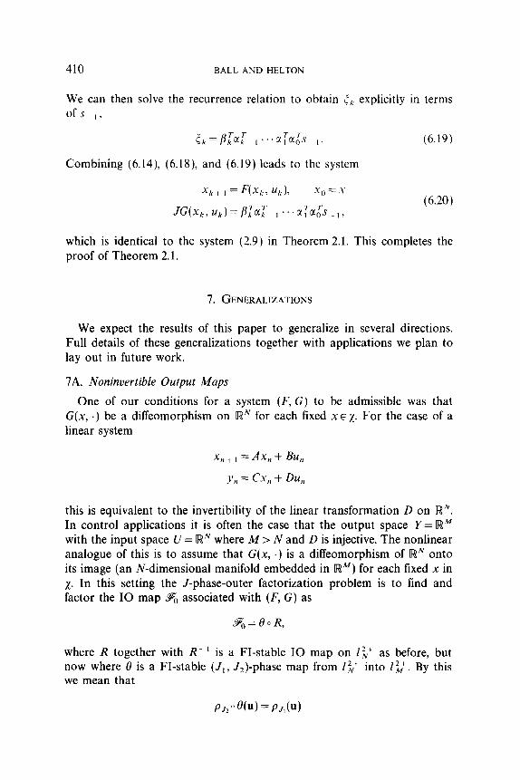
410 BALL AND HELTON

We can then solve the recurrence relation to obtain tk explicitly in terms of S-,,

(,=/?);a;~ , . ..ct.LY,rs ,. (6.19)

Combining (6.14), (6.18), and (6.19) leads to the system

(6.20)

which is identical to the system (2.9) in Theorem 2.1. This completes the proof of Theorem 2.1.

7. GENERALIZATIONS

We expect the results of this paper to generalize in several directions. Full details of these generalizations together with applications we plan to lay out in future work.

7A. Noninvertible Output Maps

One of our conditions for a system (J’, G) to be admissible was that G(x, .) be a diffeomorphism on R”’ for each fixed x E x. For the case of a linear system

X n+,=Ax,+Bu,,

y, = Cx, + Du,

this is equivalent to the invertibility of the linear transformation D on RN. In control applications it is often the case that the output space Y = R” with the input space U = RN where M > N and D is injective. The nonlinear analogue of this is to assume that G(x, .) is a diffeomorphism of RN onto its image (an N-dimensional manifold embedded in R”) for each fixed x in x. In this setting the J-phase-outer factorization problem is to find and factor the IO map & associated with (F, G) as

where R together with R-’ is a FI-stable IO map on I’,” as before, but now where 8 is a FI-stable (J,, J,)-phase map from Zc into lp. By this we mean that

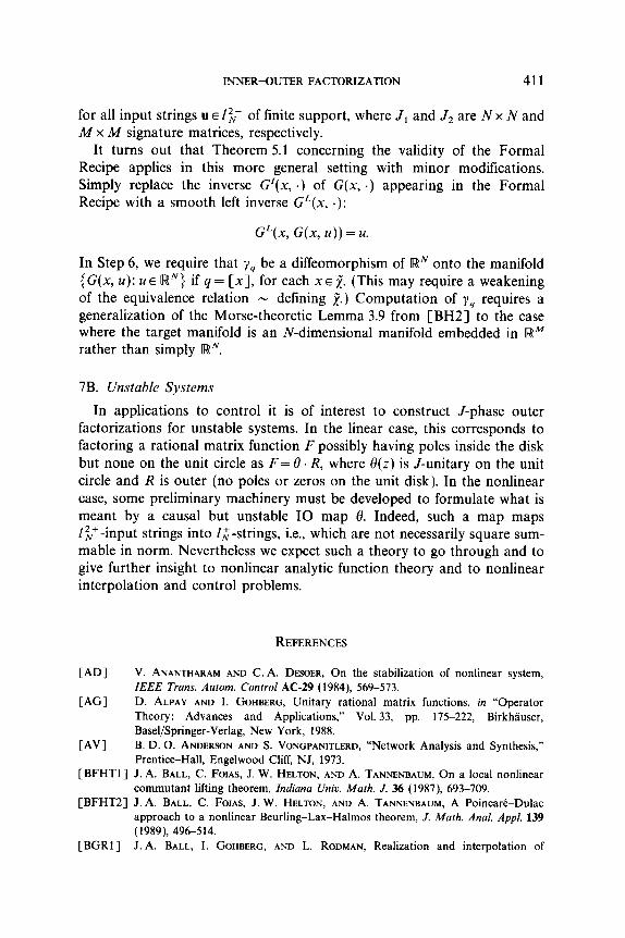
INNER+XJTER FACTORIZATION 411

for all input strings u E i’,” of finite support, where J, and J2 are N x N and A4 x A4 signature matrices, respectively.

It turns out that Theorem 5.1 concerning the validity of the Formal Recipe applies in this more general setting with minor modifications. Simply replace the inverse G’(x, .) of G(x, .) appearing in the Formal Recipe with a smooth left inverse GL(x, .):

GL(x, G(x, u)) = u.

In Step 6, we require that y4 be a diffeomorphism of IWN onto the manifold { G(x, u): UE RN} if q= [xl, for each XE i. (This may require a weakening of the equivalence relation - defining j.) Computation of yq requires a generalization of the Morse-theoretic Lemma 3.9 from [BH2] to the case where the target manifold is an N-dimensional manifold embedded in [W”” rather than simply IWN.

7B. Unstable Systems

In applications to control it is of interest to construct J-phase outer factorizations for unstable systems. In the linear case, this corresponds to factoring a rational matrix function F possibly having poles inside the disk but none on the unit circle as F= (3. R, where 0(z) is J-unitary on the unit circle and R is outer (no poles or zeros on the unit disk). In the nonlinear case, some preliminary machinery must be developed to formulate what is meant by a causal but unstable IO map 8. Indeed, such a map maps Z2,f -input strings into I,+-strings, i.e., which are not necessarily square summable in norm. Nevertheless we expect such a theory to go through and to give further insight to nonlinear analytic function theory and to nonlinear interpolation and control problems.

REFERENCES

CAD1

CAGI

CAW

V. ANANTHARAM AND C. A. DESOER, On the stabilization of nonlinear system, IEEE Trans. Autom. Control AC-29 (1984), 569-513. D. ALPAY AND I. GOHBERG, Unitary rational matrix functions, in “Operator Theory: Advances and Applications,” Vol. 33, pp. 175-222, Birkhauser, Basel/Springer-Verlag, New York, 1988. B. D. 0. ANDERSON AND S. VONGPANITLERD, “Network Analysis and Synthesis,” Prentice-Hall, Engelwood Cliff, NJ, 1973.

[BFHTl] J. A. BALL, C. FOIAS, J. W. HELTON, AND A. TANNENBAUM, On a local nonlinear commutant lifting theorem, Indiana Uniu. Mafh. J. 36 (1987), 693-709.

[BFHT2] J. A. BALL, C. FOIAS, J. W. HELTON, AND A. TANNENBAUM, A Poincari-Dulac approach to a nonlinear Beurling-Lax-Halmos theorem, J. Math. Anal. Appl. 139 (1989), 496514.

[BGRl] J. A. BALL, I. GOHBERG, AND L. RODMAN, Realization and interpolation of

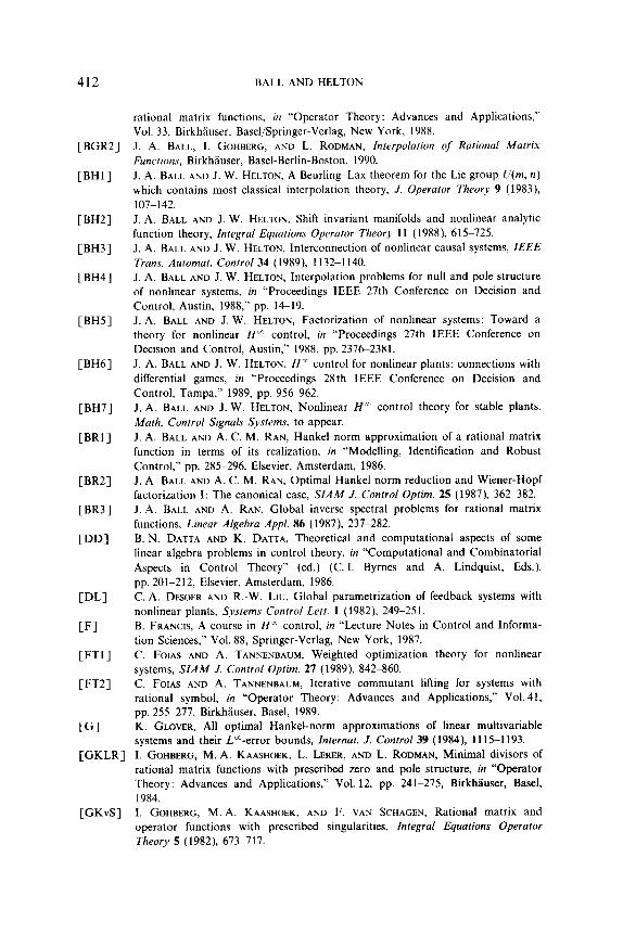
412

[BGRZ]

WHll

[BH21

IBH31

BH4]

BH5]

BH6]

CBH’II

CBRll

CBR21

IBR31

IDDI

W-1

CFI

CFTll

W-21

CGI

[GKLR]

[GKvS]

BALL AND HELTON

rational matrix functions, in “Operator Theory: Advances and Applications,” Vol. 33, Birkhtiuser, Basel/Springer-Verlag, New York, 1988. J. A. BALL, I. GOHBERG, AND L. RODMAN, Interpolation of Rational Matrix Funcrions, Birkhluser, Basel-Berlin-Boston, 1990. J. A. BALL AND J. W. HELTON, A Beurling-Lax theorem for the Lie group U(m, n) which contains most classical interpolation theory, J. Operator Theory 9 (1983), 107-142. J. A. BALL AND J. W. HELTON, Shift invariant manifolds and nonlinear analytic function theory, Integral Equations Operator Theory 11 (1988), 615-725. J. A. BALL AND J. W. HELTON, Interconnection of nonlinear causal systems, ZEEE Trans. Automat. Control 54 (1989), 1132-1140. J. A. BALL AND J. W. HELTON, Interpolation problems for null and pole structure of nonlinear systems, in “Proceedings IEEE 27th Conference on Decision and Control, Austin, 1988,” pp. 1419. J. A. BALL AND J. W. HELTON, Factorization of nonlinear systems: Toward a theory for nonlinear H” control, in “Proceedings 27th IEEE Conference on Decision and Control, Austin,” 1988, pp. 23762381. J. A. BALL AND J. W. HELTON, H” control for nonlinear plants: connections with differential games, in “Proceedings 28th IEEE Conference on Decision and Control, Tampa,” 1989, pp. 956962. J. A. BALL AND J. W. HELTON, Nonlinear H” control theory for stable plants, Math. Control Signals Systems, to appear. J. A. BALL AND A. C. M. RAN, Hankel norm approximation of a rational matrix function in terms of its realization, in “Modelling, Identification and Robust Control,” pp. 285-296. Elsevier, Amsterdam, 1986. J. A. BALL AND A. C. M. RAN, Optimal Hankel norm reduction and Wiener-Hopf factorization 1: The canonical case, SIAM J. Control Optim. 25 (1987), 362-382. J. A. BALL AND A. RAN, Global inverse spectral problems for rational matrix functions, Linear Algebra Appl. 86 (1987), 237-282. B. N. DA~TA AND K. DATTA, Theoretical and computational aspects of some linear algebra problems in control theory, in “Computational and Combinatorial Aspects in Control Theory” (ed.) (C. 1. Byrnes and A. Lindquist, Eds.), pp. 201-212, Elsevier, Amsterdam, 1986. C. A. DESOER AND R.-W. Lru, Global parametrization of feedback systems with nonlinear plants, Systems Control Left. 1 (1982), 249-251. B. FRANCIS, A course in H” control, in “Lecture Notes in Control and lnforma- tion Sciences,” Vol. 88, Springer-Verlag, New York, 1987. C. FOIAS AND A. TANNENBAUM, Weighted optimization theory for nonlinear systems, SIAM J. Control Opfim. 27 (1989), 842-860. C. FOIAS AND A. TANNENBAUM, Iterative commutant lifting for systems with rational symbol, in “Operator Theory: Advances and Applications,” Vol. 41, pp. 255-277. Birkhsuser, Basel, 1989. K. CLOVER, AI1 optimal Hankel-norm approximations of linear multivariable systems and their L”-error bounds, Infernat. J. Control 39 (1984), 1115-1193. I. GOHBERG, M. A. KAASHOEK, L. LERER, AND L. RODMAN, Minimal divisors of rational matrix functions with prescribed zero and pole structure, in “Operator Theory: Advances and Applications,” Vol. 12, pp. 241-275, Birkhiiuser, Base], 1984. I. GOHBERG, M. A. KAASHOEK, AND F. VAN SCHAGEN, Rational matrix and operator functions with prescribed singularities, Integral Equations Operafor Theory 5 (1982), 673-717.

INNER4UTER FACTORIZATION 413

WI

[II

WI

CJI

IKI [MATL]

CNFI

CPOSI CRRI

IS1

J. W. HELTON, ET AL., Opertor theory, analytic functions, matrices and electrical engineering, in “Regional Conference Series in Mathematics,” ISSN 0160-7642, No. 68, Amer. Math. Sot., Providence, RI, 1987. A. ISIDORI, “Nonlinear Control Systems: An Introduction,” Springer-Verlag, Berlin/Heidelberg/New York, 1985. A. ISIDORI AND C. H. Moot, On the nonlinear equivalent of the notion of transmission zeros, in “Modeling and Adaptive Control” (C. I. Byrnes and A. H. Kurzanski, Eds.), Lecture Notes in Control and Information Sciences, Vol. 105, pp. 146158, Springer-Verlag, New York, 1988. B. JAKUBCZYK, Existence and uniqueness of realizations of nonlinear systems, SIAM J. Control Optim. 18 (1980), 455471. T. KAILATH, “Linear Systems,” Prentice-Hall, Englewood Cliffs, NJ, 1980. MATLAB Robust Control Tool Box. B. SZ.-NAGY AND C. FOIAS, “Harmonic Analysis of Operators on Hilbert Space,” North-Holland, Amsterdam, 1970. I. POSTLETHWAITE, University of Oxford. M. ROSENBLUM AND J. R. ROVNYAK, “Hardy Classes and Operator Theory,” Oxford Univ. Press, London, 1985. H. J. SUSSMANN, Existence and uniqueness of minimal realizations of nonlinear systems, Math. Systems Theory 10 (1977), 263-284.

580 lW?-I2

inner-outer factorization of nonlinear operators*

Documents