inna thesis final version ok5 - usirusir.salford.ac.uk/30249/1/kholidasari.inna_thesis_2013.pdf ·...
TRANSCRIPT

THE IMPLICATIONS OF JUDGEMENTAL INTERVENTIONS INTO AN INVENTORY
SYSTEM
Inna KHOLIDASARI
PhD Thesis 2013

THE IMPLICATIONS OF JUDGEMENTAL INTERVENTIONS INTO AN INVENTORY
SYSTEM
Inna KHOLIDASARI
Salford Business School College of Business & Law
University of Salford, Salford, UK
Submitted in Partial Fulfilment of the Requirements Of the Degree of Doctor of Philosophy
September 2013

i
Table of Contents
Table of Contents ............................................................................................................... i
List of Figures .................................................................................................................. vi
List of Tables ................................................................................................................. viii
Abstract ............................................................................................................................. x
Acknowledgements .......................................................................................................... xi
Dedication ....................................................................................................................... xii
Declaration ..................................................................................................................... xiii
Chapter 1. INTRODUCTION ........................................................................................... 1
1.1. Outline ................................................................................................................... 1
1.2. Research background ............................................................................................. 1
1.3. Need for the research ............................................................................................. 4
1.4. Aim and objectives ................................................................................................ 7
1.5. The structure of the thesis ...................................................................................... 8
Chapter 2. AN OVERVIEW OF INVENTORY SYSTEMS ......................................... 10
2.1. Introduction .......................................................................................................... 10
2.2. Demand categorisation ........................................................................................ 12
2.2.1. ABC classification scheme ........................................................................... 13
2.2.2. Demand characteristics ................................................................................. 14
2.3. Forecasting ........................................................................................................... 19
2.3.1. Quantitative methods .................................................................................... 21
2.3.1.1. Simple Moving Average (SMA) ............................................................ 21
2.3.1.2. Exponentially Weighted Moving Average (EWMA) ............................ 22
2.3.1.3. Croston’s method ................................................................................... 22
2.3.1.4. Syntetos-Boylan approximation (SBA) ................................................. 25
2.3.1.5. Teunter-Syntetos-Babai (TSB) method ................................................. 26

ii
2.3.1.6. Bootstrapping method ............................................................................ 27
2.3.2. Qualitative methods ...................................................................................... 29
2.4. Forecasting support systems (FSS) ...................................................................... 30
2.5. Stock control system ............................................................................................ 32
2.6. Conclusions .......................................................................................................... 39
Chapter 3. JUDGEMENTAL ADJUSTMENTS IN AN INVENTORY SYSTEM ....... 40
3.1. Introduction .......................................................................................................... 40
3.2. Judgemental adjustments in SKU classification .................................................. 41
3.3. Judgemental adjustments in forecasting .............................................................. 42
3.3.1. Laboratory studies ......................................................................................... 42
3.3.2. Empirical studies ........................................................................................... 44
3.4. The relevance of human intervention in forecasting ........................................... 46
3.5. Combining forecast procedures ........................................................................... 51
3.6. The robustness of Simple Moving Average (SMA) method ............................... 54
3.7. Judgemental adjustments of inventory parameters .............................................. 56
3.7.1. Laboratory inventory studies ........................................................................ 56
3.7.2. Empirical inventory studies .......................................................................... 58
3.8. Learning and forgetting effects in manufacturing systems .................................. 59
3.9. The need for a new paradigm of inventory management .................................... 64
3.10. Enterprise Resource Planning ............................................................................ 70
3.10.1. MaterialManagement module ..................................................................... 71
3.11. Theoretical framework ....................................................................................... 72
3.12. Conclusions ........................................................................................................ 73
Chapter 4. RESEARCH METHODOLOGY .................................................................. 75
4.1. Introduction .......................................................................................................... 75
4.2. Case organisation ................................................................................................. 75
4.2.1. ERP system in case organisation .................................................................. 77

iii
4.2.2. Empirical data ............................................................................................... 77
4.2.2.1. SKUs classification ................................................................................ 78
4.2.2.2. Forecasting and stock control ................................................................ 79
4.2.3. Judgemental adjustment process ................................................................... 84
4.3. Construction of the database ................................................................................ 87
4.4. Detailed research questions ................................................................................. 93
4.5. Research classification ....................................................................................... 100
4.6. Research methodology ....................................................................................... 101
4.6.1. Research philosophy ................................................................................... 101
4.6.2. Research approach ...................................................................................... 104
4.6.3. Research strategy ........................................................................................ 107
4.6.4. Research choice .......................................................................................... 108
4.6.5. Time horizons ............................................................................................. 109
4.6.6. Research techniques .................................................................................... 110
4.7. Conclusions ........................................................................................................ 110
Chapter 5. EMPIRICAL DATA ANALYSIS AND FINDINGS ................................. 112
5.1. Demand descriptive statistics ............................................................................. 112
5.2. Price of the SKUs .............................................................................................. 114
5.3. Analysis of judgemental adjustments ................................................................ 118
5.3.1. Goodness-of-fit tests and distributional considerations .............................. 120
5.4. Analysis of the justification of adjustments ....................................................... 127
5.5. Simulation experiment ....................................................................................... 133
5.5.1. Conceptual model of simulation ................................................................. 134
5.5.2. Validation and verification of the simulation model .................................. 136
5.5.3. Simulation results ....................................................................................... 138
5.6. The effects of the sign of adjustments on inventory performance ..................... 141
5.7. The effects of the absolute size of adjustments on inventory performance ....... 146
iv
5.7.1. The average of the absolute size of the adjustments ................................... 146
5.7.2. The absolute average size of the adjustments ............................................. 149
5.8. The effects of justification of adjustments on inventory performance .............. 153
5.9. The effect of bias of adjustments on inventory performance ............................ 157
5.10. Learning effects of making adjustments on inventory performance ............... 161
5.11. The combination methods of the OUT level ................................................... 165
5.12. Explanatory Power of SMA-based OUT replenishment level ......................... 168
5.13. Framework for judgmentally adjusted orders .................................................. 171
5.14. Conclusions ...................................................................................................... 173
Chapter 6. CONCLUSION, CONTRIBUTIONS, LIMITATIONS, AND FURTHER
RESEARCH .................................................................................................................. 177
6.1. Introduction ........................................................................................................ 177
6.2. Conclusions ........................................................................................................ 178
6.3. Implications ....................................................................................................... 183
6.3.1. Implications for the OM theory .................................................................. 183
6.3.2. Implications for the OM practice ................................................................ 184
6.4. Limitations ......................................................................................................... 186
6.4.1. Generalisation of theory .............................................................................. 186
6.4.2. Interviews with the manager ....................................................................... 187
6.4.3. Construction of the database and simulation experiment ........................... 187
6.4.4. Goodness-of-fit distribution tests ................................................................ 188
6.5. Further research ................................................................................................. 188
BIBLIOGRAPHY ......................................................................................................... 190
Appendix A: Forecasting methods for fast-moving forecasting ................................... 206
Appendix B: ERP .......................................................................................................... 209
Appendix C: WEEE Directive ...................................................................................... 215
Appendix D: RoHS Directive ....................................................................................... 218

v
Appendix E: The results of goodness of fit test of Final OUT replenishment level
adjustment distribution across SKUs ............................................................................ 220
Appendix F: Results of fitting distribution test on Final OUT replenishment level across
period ............................................................................................................................ 223
Appendix G: Explanation of reason categories ............................................................ 225
Appendix H – List of Code ........................................................................................... 227

vi
List of Figures
Figure 1.1 The incorporation of human judgement into an inventory system .................. 3
Figure 1.2 The organisation of the thesis .......................................................................... 9
Figure 2.1 An overview of a typical inventory system ................................................... 11
Figure 2.2 Williams’ categorisation scheme .................................................................. 15
Figure 2.3 Eaves’ categorisation scheme ........................................................................ 16
Figure 2.4 Syntetos and Boylan categorisation scheme ................................................. 18
Figure 3.1 Classification of methodology in operation management research. .............. 66
Figure 3.2 Theoretical framework of the research .......................................................... 73
Figure 4.1 RAW sheet of original data ........................................................................... 79
Figure 4.2 Data calculation sheet for original data ......................................................... 82
Figure 4.3 Stock control system for A items .................................................................. 83
Figure 4.4 Stock control system for B items .................................................................. 83
Figure 4.5 An example of the adjustment process .......................................................... 86
Figure 4.6 The process of adjustments to the OUT level. .............................................. 86
Figure 4.7 NEW ROP sheet of original data .................................................................. 87
Figure 4.8 Compiling information into a time-series format .......................................... 88
Figure 4.9 Complete database over time ........................................................................ 89
Figure 4.10 Weekly demand data for whole time horizons ............................................ 90
Figure 4.11 Original data of detailed OUT level ............................................................ 91
Figure 4.12 Detailed ROP for whole time horizons ....................................................... 92
Figure 4.13 Complete database for A items ................................................................... 93
Figure 4.14 Philosophical positioning of the research .................................................. 104
Figure 4.15An integrated (semi-deductive) research approach .................................... 105
Figure 4.16The research approach in detail .................................................................. 106

vii
Figure 4.17 Research choices ....................................................................................... 108
Figure 4.18 The research onion of this work ................................................................ 111
Figure 5.1 The distribution of average inter-demand interval for A items. .................. 114
Figure 5.2 Distribution of material price for A items ................................................... 117
Figure 5.3 Distribution of material price for B items ................................................... 117
Figure 5.4 Distribution of the signed size of adjustments for A items ......................... 121
Figure 5.5 Distribution of the absolute size of adjustments for A items ...................... 122
Figure 5.6 Distribution of the relative signed size of adjustments for A items ............ 122
Figure 5.7 Distribution of the relative absolute size of adjustments for A items ......... 123
Figure 5.8 Distribution of the signed size of adjustments for B items ......................... 124
Figure 5.9 Distribution of the absolute size of adjustments for B items ...................... 124
Figure 5.10 Distribution of the relative signed size of adjustments for B items .......... 125
Figure 5.11 Distribution of the relative absolute size of adjustments for B items ....... 125
Figure 5.12 Slope of demand pattern ............................................................................ 128
Figure 5.13 Comparison between trends and reason for judgement made by manager 129
Figure 5.14 Example of inconsistency (the reason for making an adjustment is
‘decreasing demand’ while the demand is increasing over time) .............. 130
Figure 5.15 Example of inconsistency (the reason for making an adjustment is
‘increasing demand’ while the demand is decreasing over time) .............. 130
Figure 5.16 Distribution of adjustments per justification category (A items) .............. 132
Figure 5.17 Distribution of adjustments per justification category (A items) .............. 133
Figure 5.18 Verification and validation of the simulation model ................................. 138
Figure 5.19 A framework to facilitate the process of judgemental adjustments .......... 172

viii
List of Tables
Table 3.1 Comparison of the Traditional and the New Paradigm .................................. 66
Table 3.2 Model assumptions and possible behavioural gaps in inventory and supply
chain management. ...................................................................................... 68
Table 3.3. Function of MM sub-menus. ........................................................................ 71
Table 4.1 Classification of main types of research ....................................................... 100
Table 4.2 Contrasting positivist and interpretivist ........................................................ 103
Table 4.3 Relevant situations for different research methods ...................................... 107
Table 4.4 Dimension of contrast among the three research choices ............................. 109
Table 5.1 Demand data series characteristics for A items ............................................ 113
Table 5.2 Demand data series characteristics for B items ............................................ 113
Table 5.3 Spare parts prices for A items and B items. .................................................. 115
Table 5.4 Theoretical distributions being tested ........................................................... 120
Table 5.5 Adjustment distributions for A items and B items. ...................................... 126
Table 5.6 Number of adjustments per justification category(A items) ......................... 131
Table 5.7 Number of adjustments per justification category(B items) ......................... 132
Table 5.8 The simulation results for A items ................................................................ 140
Table 5.9 The simulation results for B items ................................................................ 140
Table 5.10 The effect of sign adjustments on inventory performance for A items ...... 143
Table 5.11 The results of sign adjustments on inventory performance for B items ..... 143
Table 5.12 The results of absolute of adjustment on the inventory performance analysis
for A items ................................................................................................. 148
Table 5.13 The results of absolute of adjustment on the inventory performance analysis
for B items .................................................................................................. 148

ix
Table 5.14 The results of absolute signed of adjustments on the inventory performance
analysis for A items ................................................................................... 151
Table 5.15 The effects of absolute signed of adjustments for B items ......................... 151
Table 5.16 The results of justification of adjustments on the inventory performance
analysis for A items ................................................................................... 155
Table 5.17 The results of justification of adjustments on the inventory performance
analysis for B items .................................................................................... 155
Table 5.18 The results of the bias of adjustments on the inventory performance analysis
for A items ................................................................................................. 160
Table 5.19 The results of the biased on adjustments on the inventory performance
analysis for B items .................................................................................... 160
Table 5.20 The results of learning-effects analysis based on number of adjustments for
A items ....................................................................................................... 163
Table 5.21 The results of learning-effects analysis based on number of adjustments for
B items ....................................................................................................... 163
Table 5.22 The simulation results for A and B items ................................................... 167
Table 5.23 Data of SMA-based OUT replenishment levels and Final OUT
replenishment levels for material XB0306001 .......................................... 169
Table 5.24. Summary output of regression analysis of material XB0306001 .............. 169
Table 5.25 The descriptive statistic of P value for A and B items ............................... 170
x
Abstract
Physical inventories constitute a considerable proportion of companies’ investments in
today’s competitive environment. The trade-off between customer service levels and
inventory investments is addressed in practice by formal quantitative inventory
management (stock control) solutions. Given the tremendous number of Stock Keeping
Units (SKUs) that contemporary organisations deal with, such solutions need to be fully
automated. However, managers very often judgementally adjust the output of statistical
software (such as the demand forecasts and/or the replenishment decisions) to reflect
qualitative information that they possess. In this research we are concerned with the
value being added (or not) when statistical/quantitative output is judgementally adjusted
by managers. Our work aims to investigate the effects of incorporating human
judgement into such inventory related decisions and it is the first study to do so
empirically. First, a set of relevant research questions is developed based on a critical
review of the literature. Then, an extended database of approximately 1,800 SKUs from
an electronics company is analysed for the purpose of addressing the research questions.
In addition to empirical exploratory analysis, a simulation experiment is performed in
order to evaluate in a dynamic fashion what are the effects of adjustments on the
performance of a stock control system.
The results on the simulation experiment reveal that judgementally adjusted
replenishment orders may improve inventory performance in terms of reduced inventory
investments (costs). However, adjustments do not seem to contribute towards the
increase of the cycle service level (CSL) and fill rate. Since there have been no studies
addressing similar issues to date, this research should be of considerable value in
advancing the current state of knowledge in the area of inventory management. From a
practitioner’s perspective, the findings of this research may guide managers in adjusting
order-up-to levels for the purpose of achieving better inventory performance. Further,
the results may also contribute towards the development of better functionality of
inventory support systems (ISS).

xi
Acknowledgements
I would like to thank the following people and organisations for supporting me in
numerous ways throughout my PhD.
First and foremost, I would like to express my wholehearted gratitude to Prof. Aris A.
Syntetos, my supervisor, for his patience and his constant support and guidance
throughout the period of my Ph.D. study.
I would like to thank the Ministry of National Education and Culture, Government of
Indonesia, for providing the scholarship for my Ph.D and the Salford Business School,
University of Salford for all the support and facilities.
Special thanks to my friends in Maxwell 528, Dima, Wenjia, Asif, Ila, Rossi, Katie,
Afaf and Sira for all their wonderful friendship during the last four years. Many thanks
to my best friend Dave, the one who knows what I need more than myself.
Also, many thanks and love to my family; Ibu, Bapak, Mama, Papa, Dhida, Yanna,
Affan for all their love, encouragement and for always praying for me.
Love to my lovely children Afif and Hanhan for bringing so much happiness and
strength to my life. Finally, I would like to thank, with much respect, my amazing
husband Taufika Ophiyandri for his continuing support, patience, encouragement for all
my work and for his loving care, sacrificing of his valuable time and his commitment to
my achievements.

xii
Dedication
I dedicate this piece of work to my dearest husband Bang Phy & my lovely children Afif and Hanhan

xiii
Declaration
This thesis is submitted under the University of Salford requirements for the award of a
PhD degree by research. Some research findings were published in refereed conference
proceedings prior to the submission of the thesis during the period of PhD studies.
The researcher declares that no portion of the work referred to in the thesis has been
submitted in support of an application for another degree or qualification to the
University of Salford or any other institution.
Inna Kholidasari

1
Chapter 1. INTRODUCTION
1.1. Outline
This research is concerned with the effects of incorporating human judgement into
inventory-related decisions. In particular, we1 focus on the case of service/spare parts
inventories. This introductory chapter describes the motivation behind this research by
placing the study in a business context. Section 1.2 discusses the research background,
followed by the need for the research in Section 1.3. The aim and objectives of the research
are given in Section 1.4. Finally, Section 1.5 focuses on the structure of this thesis.
1.2. Research background
Physical inventories constitute a considerable proportion of companies’ investments in
today’s competitive environment. According to the 22nd Annual State of Logistics Report,
the world is currently sitting on approximately $8 trillion worth of goods held for sale
(Wilson, 2011). About 10% of that value relates to spare parts; according to US Bancorp,
spare parts relate to a $700 billion annual expenditure, constituting about 8% of the US
gross domestic product (Jasper, 2006). Mobley (2002) argues that maintenance costs
typically account for 15-60% of the total value of an end product, validating the figures
presented above with regards to spare parts expenditure. The following statistics are also
relevant: two relatively recent reports by the Aberdeen Group (2005) and Deloitte (2006)
1The use of the word “we” throughout the thesis is purely conventional. The work presented in this PhD thesis is the result of research conducted by the author alone, albeit with support from an academic institution.

2
identify the increasing importance of the spare parts business. As stated in the latter report,
the combined revenues of many of the world's largest manufacturing companies are more
than US$1.5 trillion. Furthermore, on average, service revenues account for more than 25%
of the total business. To the best of our knowledge, such figures have not been published
for the United Kingdom alone, but based on the above it is clear that small improvements
regarding the management of maintenance and of spare parts may be translated into
substantial cost savings, with a considerable contribution to the country’s economy.
Moreover, inventories play an important role in improving the service level and reducing
the operation cost of logistic systems. Companies strive to ensure high customer
satisfaction, and off-the-shelf availability is almost a necessity under current supply chain
arrangements. The trade-off between customer service levels and inventory investment is
addressed in practice by formal quantitative inventory management (stock control)
solutions. Commonly, an inventory system consists of a three-stage process. Firstly, stock-
keeping units (SKUs) are classified into various categories based on some common
characteristics (such as underlying demand patterns, volume of sales, price, importance,
etc.). Next, specific methods are used for each category in order to extrapolate
requirements into the future. Finally, various stock control formulations are employed in
order to convert the forecasts into inventory decisions (when and how much to order).
Given the tremendous number of SKUs that contemporary organisations deal with, the
solutions need to be fully automated. However, although such systems are indeed in
principle fully automated, what most often happens in practice is this: managers intervene
in the system and use their judgement to adjust or decide on various quantitative elements.
For example, they may impose fully subjective (experience-driven) criteria for the purpose
of classifying an SKU, based on demand frequency, demand value, or the criticality of the
items being classified (Silver et al., 1998; Naylor, 1996). Also, managers often set the

3
boundaries of SKU classification in an arbitrary way (e.g. William, 1984; Eaves, 2002),
despite the existence of more logically coherent approaches such as those proposed by
Johnston and Boylan (1996) and Syntetos and Boylan (2005). Even more frequently, they
judgementally adjust a statistical forecast or a replenishment decision. If, for example, the
forecast produced by the system for a particular SKU is 10 units, then a manager may
introduce some qualitative information and amend the forecast to, say, 15 units, thus
overriding the system. Similarly, a replenishment decision of 15 units may be reduced to
reflect additional information available to the manager, about, for example, some increased
competition (due to a competitor reducing their prices) likely to occur in the near future.
The process discussed above is depicted in the following figure (Figure 1.1).
Figure 1.1 The incorporation of human judgement into an inventory system
Although there is a growing body of empirical knowledge in the area of judgementally
adjusting statistical forecasts, there has been little discussion about judgemental
adjustments neither to SKU classification; nor at the moment there a single empirical study
that explores the effects of such judgemental adjustments into replenishment decisions.
This is most important in terms of developing our understanding of the process of training
provision and design of decision support systems. All these issues are discussed later on in
this thesis in more detail.
Inventory system
Forecasting Classification of SKUs
Stock control
Judgement
Stock holding cost
CSL
Judgement Judgement

4
1.3. Need for the research
Because of the tremendous number of SKUs that both manufacturing and service
organisations deal with, it is clear that the inventory task needs to be automated.
Automation here implies fully quantitative models that can run on their own without
human intervention, thus relying upon statistical, generalisable principles. Such models
rely upon past information that is available to the system and thus may not of course
capture contextual knowledge that managers may possess. For example, experts/managers
may know that institutions are in the process of change, or that a product promotion is
about to take place, that certain actions are being undertaken by competitors that will affect
demand for the product, or that a manufacturing problem exists. The impact of these events
is specific, and cannot be included in the model being used. Similarly, a variable that is
difficult to measure may be missing from the model. Judgement may be used when
insufficient data is available to support statistical methods, or situations arise where
exceptional events are known to be occurring in the future. In practice, managers adjust the
output of automated systems by altering some quantities, and this is not necessarily a bad
thing. As Soergel (1983) and Jenks (1983) pointed out, it is judgement alone that can
anticipate one-time events which, if not accounted for, could have severe negative
consequences for the organisation.
Many studies have discussed the effect of human intervention on statistical forecasting
models. For example, Cerullo and Avila (1975) surveyed 110 large companies and found
that 89% used judgemental forecasting alone or a combination of judgement and a formal
model. Klein and Linneman (1984) surveyed 500 of the world’s largest corporations and
found that the overwhelming majority of corporate planners identified severe limitations in
using purely statistical techniques. A survey of corporations in the United States (Sanders
and Manrodt, 1994) found that 57% of respondents always used judgemental methods, and

5
21% did so frequently. Furthermore, 45% of the respondents said that they always adjusted
their statistical forecasts and 37% did so sometimes. In a study of Canadian firms, Klassen
and Flores (2001) reported that 80% of the respondents that used computer-based forecasts
used judgement to adjust them.
A plethora of studies look at this phenomenon in regards to forecasting. However, in terms
of inventory systems, practitioners often adjust the stock replenishment order, not the
forecast. Kolassa et al. (2008) report that judgemental adjustments of stock control
quantities occurs more often than forecast-related adjustments.
A distinction needs to be made at this point between: i) solely employing judgement as a
means of predicting the future, and ii) the use of quantitative methodologies adjusted by
managers in order to reflect qualitative information. In this research we refer to the latter,
and although there are numerous studies that look at this phenomenon when it comes to
forecasting, there are no studies at all that examine: i) the effects of judgementally
adjusting classification rules, ii) the effects of judgementally adjusting replenishment
decisions, and iii) the cumulative effect of adjusting more than one aspect of the system
under concern. In this research we are concerned with the effects of judgement on
replenishment decisions.
This constitutes precisely the purpose of this PhD research, which aims at analysing the
effects of judgemental adjustments into inventory control. Since this research includes
elements of Operations Management (OM)/Operational Research (OR) and behavioral
aspects of decision-making, it should contribute and advance knowledge in the field of
behavioural operations. Croson et al. (2013) argued that research in behavioural operations
analyses decisions and the behaviour of individuals/small groups of individuals to gain a
deeper understanding of operations processes, and make better recommendations on how
to design and improve the operations processes. Furthermore, Bendoly et al. (2006)

6
reported that this field of study should be very much associated with inventory
management and production management; however, this is the first study that attempts to
do so and currently (and as discussed above), to the best of our knowledge, there is not a
single paper in the academic literature that addresses this issue.
We do so by means of analysing an extended empirical database coming from the
electronics industry. Managers in the company under consideration adjust inventory
quantities, often providing a qualitative justification for their action. Linking the effects of
adjustments to the justification provided for such adjustments has never been discussed in
the academic literature before; this linkage (on its own) is perceived as a major
contribution of the thesis.
The fact that this work is based on a single case can be justified partly by the lack of any
previous research in this area, but mostly on the sensitivity of the information required to
perform such a study. Adjustments reflect a manager’s personal opinion and such data
cannot be easily retrieved. In addition, and as will be explained later in this report, the very
construction of the database was a very difficult exercise since the company provided only
fragmented information which needed to be constructively put together.
The company under discussion represents the European logistics operations of a major
international electronics manufacturer. The entire database relates to service parts used for
supporting the final pieces of equipment (such as printers) sold in Europe. This category of
items is very difficult to control as the majority of these items are in very low (intermittent)
demand and tend to be expensive due to high stock investments (Martin et al., 2010). The
researchers under concern reported that the quantitative models and forecasting techniques
described in the literature are not sufficient to control spare/service parts inventories and
new avenues for contribution in this area should emphasise the qualitative aspects of the
problem as well. The same of course is true for all intermittent demand items; although the

7
database available for the purposes of this research relates to service parts, there is a safe
extension of our discussion and findings to all intermittent demand products.
1.4. Aim and objectives
This study aims to explore the effects of incorporating human judgement into inventory
decision-making. From a theoretical perspective there is tremendous scope for contributing
and further advancing the current state of knowledge, since there have been no studies
addressing this issue to date. From a practitioner’s perspective, the findings of this research
result into tangible suggestions and recommendations to inventory managers of service
parts and beyond, in addition to the obvious implications for decision support systems
design and improvement.
The aim of the research is reflected in the following objectives:
1. To critically review the literature on how judgement relates to the main functions of an
inventory system.
2. To assess the implications of judgemental adjustments on real data, focusing on
replenishment orders.
3. To link the performance of adjustments with the managers’ justification for introducing
such adjustments in the first place.
4. To understand for the first time how managers adjust inventory-related decisions.
5. To evaluate the circumstances under which human judgement leads to performance
improvement.
6. To derive a number of insights with regard to practical applications and a number of
suggestions for improving the functionality of software packages.

8
1.5. The structure of the thesis
The remainder of this thesis is organised as follow:
Chapter 2 provides a literature review of issues related to demand categorisation,
forecasting and stock control. Each element of the inventory management system is
presented under a separate section of the chapter. The literature review focuses on the
intermittent demand context since the empirical data used in this research relates to
service/spare parts. Such SKUs are known to be almost invariably characterized by
intermittent demand structures.
In Chapter 3 the issue of judgemental adjustments into an inventory system is discussed.
The relevant part of the forecasting literature is widely reviewed along with the very few
contributions that have emphasized demand categorisation as well as stock control. This
chapter also discusses learning and forgetting effects in the manufacturing domain
(because of its relevance to the focus of this research), and presents a state of the art into
the new paradigm of inventory management. Information about enterprise resource
planning (ERP) systems is also provided as this links to the case organisation. The
company under concern perform inventory management under an ERP solution and in that
respect a clear understanding of how such solutions operate (in particular with regards to
inventory management) is viewed as imperative to provide. Finally, a theoretical
framework for this research is also presented.
Chapter 4 outlines the case organisation, the construction of the empirical database used
for experimentation purposes and the research questions developed to guide the
experimental part of the empirical investigation. The research methodology is also
discussed in detail in this chapter.
In Chapter 5, the empirical data analysis (based on the theory of inventory systems
presented in Chapters 2 and 3, and the research questions generated in Chapter 4) is

9
discussed. A simulation experiment is developed for the purpose of addressing the research
questions.
Finally, Chapter 6 focuses on the conclusions of this research, implications of our work for
real world practices, the limitations associated with our research and important avenues for
further work in this area.
The organisation of this thesis is pictorially represented in Figure 1.2.
Figure 1.2 The organisation of the thesis
Chapter 3: Judgemental adjustments in an
inventory system
Chapter 2: An overview of inventory systems
Chapter 4: Empirical data and research methodology
Chapter 5: Empirical data analysis
Chapter 1: Background and the need for the research
Chapter 6: Conclusions, implications,
limitations and future research

10
Chapter 2. AN OVERVIEW OF INVENTORY SYSTEMS
2.1. Introduction
This chapter sets the context of our investigation by presenting an overview of the typical
operation of an inventory system. Issues related to judgemental adjustments in such a
system are discussed in detail in Chapter 3.
As discussed in the previous chapter, SKU classification, forecasting and inventory control
are important elements of an inventory system. Each element relies upon a set of
appropriate methods in order to produce the final decision. For example, with regards to
forecasting, many quantitative and qualitative models may be used. Managers/practitioners
need to decide on the most appropriate ones by considering the characteristics of demand
patterns. Alternatively, the software package may automatically select such a model.
The overview of inventory systems is depicted in Figure 2.1, followed by explanatory
discussion.

11
Figure 2.1 An overview of a typical inventory system
Demand classification methods have been extensively discussed over the years (by, for
example, Johnston and Boylan, 1996; Eaves, 2002; Syntetos and Boylan, 2005 and Teunter
et al. 2010; we return to this issue in sub-sections 2.2.1 and 2.2.2 to discuss in detail
methods of demand classification). The purpose of demand categorisation2 is to decide on
the appropriate forecasting and inventory control methods to be used for each selected
category to extrapolate requirements into the future and decide on replenishments actions
respectively. With regards to the forecasting task in particular, systems to support or
facilitate such a task (forecasting support systems, or FSS) have also been developed to
improve the performance of forecasting (selection of quantitative methods or indication of
the need for qualitative input). The output of the forecasting process constitutes the input
into stock control systems. For the performance of the entire system is then typically
reflected into two main things: inventory costs and service levels achieved.
2The words ‘categorisation’ and ‘classification’ are used interchangeably in this thesis.
Demand categorisation
Forecasting
Stock control decision
Qualitative methods
Stock control methods
FSS
Quantitative methods
Classification methods
Stock-holding cost CSL
12
In an inventory system, every stage (demand classification, forecasting, and stock control
decision-making) maybe completely automated, or parts of the process may be decided or
adjusted by managers. For example, a manager may impose particular categorisation
criteria and cut-off values, while the forecasting and stock control tasks are fully optimised
by the software in use. Alternatively, the software may be used to determine demand
categorisation and stock control decisions while forecasting operates in a semi-automated
fashion with judgemental adjustments; and all the combinations thereof. Furthermore, both
the tasks of forecasting and inventory control introduce various possibilities for human
intervention. Managers may intervene in the process of selecting the methods, or the
parameters of the methods to be used or both, in addition of course to directly adjusting
directly the forecasts or replenishment decisions themselves. In this research we are
concerned with the intervention in the final output of the system.
2.2. Demand categorisation
A demand classification scheme constitutes an essential element of an inventory system
since it benefits the decision-maker in terms of deciding the appropriate forecasting and
stock control methods to be used on the right products (Boylan et al., 2008; Syntetos et al.,
2009a). Since the organisation deals with a large number of SKUs, with a variety of
characteristics, it is not effective to evaluate them on an individual basis. SKUs with
relatively similar characteristics need to be grouped into categories in order to facilitate
decision making and allow managers to focus their attention on the most important ones.
The following sub-sections discuss issues related to demand categorisation and how
demand categorisation procedures develop, based on demand characteristics.

13
2.2.1. ABC classification scheme
Demand can be classified according to a number of factors, such as the underlying demand
characteristics, criticality, and cost. One common type is the ABC (Pareto) classification
scheme. Silver et al. (1998) explained that a Pareto report lists the SKUs in descending or
ascending order based on demand frequency, demand volumes or demand profit, and then
divides the ranked SKUs into relevant categories. Category A is assumed to consist of the
most important SKUs and therefore requires the highest service level, category B contains
SKUs of moderate importance, and relatively unimportant SKUs are placed in category C
(Lengu, 2012). However, in the spare/service parts context, the C items may become an
important or critical category if managers consider the carrying cost of such items within
the inventory. As the majority of spare/service parts are demanded in relatively low
quantities in every period (less than once per month: Teunter et al., 2010) and because
obsolescence is highly likely, such items may indeed end up being more important than A
items.
ABC classifications based on demand frequency/volume are often used in conjunction with
other criteria; the value (SKU cost × quantity required) criterion is the most commonly
applied one. Originally, the ABC classification was designed for three classes; the method
can, however, be extended to include more. For example, Syntetos et al. (2009a) addressed
the issue of demand classification for the purpose of suggesting forecasting and stock
control policies for increasing service levels and reducing stock-holding costs in an after-
sales business context. This study investigated data from a manufacturing company which
initially classified its products into six categories, based on demand frequency.
ABC classifications typically rely upon a single criterion. However, multi-criteria
classifications have been developed to account for the certainty of supply, the rate of
obsolescence, lead time, cost of review and replenishment, design and manufacturing

14
process technology, and substitutability (see e.g. Flores and Whybark, 1987; Partovi and
Burton, 1993; Buzacott, 1999; Ramanathan, 2006; Ng, 2007; Zhou and Fan, 2007; Chen et
al., 2008). Moreover, various multi-criteria methodologies have been considered, including
weighted linear programming, the analytic hierarchy process (AHP), and operation-related
groups (ORG). An alternative to multi-criteria methodologies is to use multiple way
classification, e.g. a two-way classification by purchase cost and demand value (Teunter et
al., 2010).
2.2.2. Demand characteristics
SKUs can be classified into relevant groups based on the characteristics of demand (for
example, number of orders for a particular period, demand size, and lead time between
demands). We now examine a number of studies which discuss various categorisation
procedures based on demand characteristics.
Williams (1984) proposed classification methods (for constant and variable lead time)
based on the variance of demand during lead time (DDLT). The variance of DDLT is
composed from three factors: the number of orders, the demand size of these orders and the
length of the lead times. By considering the mean lead time ��, the mean demand arrival
rate (Poisson) λ, and the squared coefficient of variation of demand sizes ������, the demand
for constant lead time (variance (L)=0) is categorised as shown in Figure 2.2 (the cutoff
values constitute a managerial input).

15
Figure 2.2 Williams’ categorisation scheme (source: Williams, 1984, pp. 942)
The intermittence of demand is indicated by ����. The higher the ratio, the more intermittent
demand is. ������ indicates the lumpiness of demand. The higher the ratio, the lumpier demand
is. Lumpiness depends on the intermittence and variability of the demand sizes. The
classified into three categories using the parameters ���� and
������: category A, and C - smooth;
category B - slow moving; category D1- sporadic; category D2- highly sporadic.
Two demand categorisation methods for non-constant lead times were developed from this
study. The first is constructed based on the size of the three summand factors discussed
above, and classifies demand into smooth, slow-moving, sporadic, and sporadic with
highly variable lead time. The second method assumes that in any lead time, demand has a
probability of being zero (p) and if it is non-zero, it equals a random variable (y). The
product is classified using p and � (squared coefficient of variation of non-zero demand)
as slow-moving demand if p>0.25 and �≤0.4 and sporadic demand if p>0.7 and c �>0.4.
This study did not intend to develop a generalised solution as the break-point values used
for the categorisation parameters were decided based on the characteristics of the particular
A C
D1
D2
B
Intermittence
0.7
2.8
0.5
���(�)��
Lumpiness

16
sample used in the study. It is therefore questionable whether this classification would be
effective when used to classify SKUs in other datasets. In addition, these break-points are
defined without considering the relative performance of different forecasting methods and
inventory policies.
Eaves (2002) developed a demand pattern classification scheme based on three lead time
demand components discussed above: i) transaction variability, ii) demand size variability,
and iii) lead-time variability. This study used demand data from the Royal Air Force
(RAF) and found that it was not sufficient to distinguish a smooth demand pattern simply
on the basis of transaction variability. Figure 2.3 shows the Eaves categorisation scheme
(that evolved from that developed by Williams, 1984) which divides demand patterns into
smooth (category A), slow-moving (category B), irregular (category C), erratic (category
D1), and highly erratic (category D2). The cutoff values were decided based on the
characteristics of the particular demand dataset and sufficient sub-sample size
considerations. The cut-off points were as follows: transaction variability: 0.74; demand
size variability: 0.10; lead time variability: 0.5.
Figure 2.3 Eaves’ categorisation scheme (source : Eaves, pp. 127)
A C
D1
D2
B
Lead-time variability
0.74
0.53
0.10
Demand size variability
Transaction variability

17
The objective of the demand categorisation methods of the above two studies was to define
the appropriate forecasting and inventory control methods for the resulting categories. The
boundaries of the demand categories were determined arbitrarily by the managers at which
point estimation procedures and stock control methods were selected in order to forecast
future requirements and manage stock efficiently.
Syntetos and Boylan (2005) established a more logical approach than that presented above,
based on the work conducted by Johnston and Boylan (1996). The demand categorisation
procedures suggested rely on the premise that is preferable to first compare alternative
forecasting (and stock control) methods for the purpose of establishing regions of superior
performance and then classify the SKUs based on the results. That is, if the purpose of
demand classification is indeed to select the most appropriate forecasting and stock control
methods, then we should start from these methods and by means of comparing them
identify regions of superior performance. Classification then naturally follows in a
meaningful manner. The work of Johnston and Boylan (1996) considered simulated Mean
Squared Errors for the purpose of comparing alternative forecasting methods (Croston’s
method (Croston, 1972) and Single Exponential Smoothing, SES) resulting in the
identification of the average inter-demand interval as an important classification parameter
(to distinguish between intermittent and non-intermittent demand). Syntetos and Boylan
(2005) took this work further by means of analysing theoretical MSE expressions and
identifying an additional classification parameter that relates to the variability of the
demand sizes, when demand occurs. The rule proposed was empirically validated on 3,000
intermittent demand series from the automotive industry.
The theoretical rule is expressed in terms of the squared coefficient of variation of the
demand sizes ( 2CV ) and the average inter-demand interval (p). The methods compared

18
were: Croston, SES and the Syntetos-Boylan Approximation (Syntetos and Boylan, 2005).
The rule results in a four-quadrant solution presented in Figure 2.4.
Figure 2.4 Syntetos and Boylan categorisation scheme (source: Syntetos et al., 2005, pp. 500 )
There is a direct suggestion now of the forecasting method to be used in each category. In
addition, the cut-off points are the outcome of a generalised analytical comparison (albeit
under specific modeling assumptions).
Kostenko and Hyndman (2006) revisited the categorisation procedure proposed by
Syntetos and Boylan (2005) in terms of some approximate simplifying assumptions that
permitted the easy four-quadrant approach presented above, and suggested a linear
function for separating between Croston and the Syntetos-Boylan Approximation (which is
discussed in detail sub-section 2.3). Heinecke et al. (2013) conducted a simulation
experiment to empirically investigate the performance of the above discussed procedures
using more than 10,000 SKUs from three different industries (electronics, military, and
automotive). The results indicated that the categorisation scheme proposed by Kostenko
Syntetos & Boylan 1
Syntetos & Boylan 2
Croston 3
Syntetos & Boylan 4
p = 1.32 (cut-off value)
CV2 = 0.49
(cut-off value)

19
and Hyndman (2006) performed well but it is questionable whether the small gains in
accuracy improvement worth the additional complexity of the scheme.
Syntetos et al. (2009a) conducted a study on demand categorisation for a European spare
parts logistics network, in order to facilitate decision making with respect to forecasting
and stock control, and to enable managers to focus their attention on the most important
SKUs. This research considered the cumulative demand frequency versus cumulative
demand value (demand value = SKU cost × quantity required) as a demand classification
parameter. This scheme resulted in six categories of items with each category being
associated with a specific treatment in terms of forecasting and stock control.
Syntetos et al. (2010a) suggested that it is important for organisations to classify their
SKUs in order to assign higher service-level targets to some critical-item categories and
identify obsolete SKUs that are very slow moving. In that study, the researchers conducted
a demand categorisation of 2,156 SKUs using the ABC (Pareto) classification based on
their contribution to profit (sales volumes × net profit). The results revealed the scope for
improving the system through increased managerial attention to the best selling items and
also to obsolete SKUs.
2.3. Forecasting
Forecasting is the process of making predictions about events that will happen in the
future. In business, demand forecasting is the basis for all planning and control activities.
In an inventory context, based on the underlying demand patterns of products, forecasting
procedures are generally divided into fast-moving and slow-moving demand methods.
Fast-moving demand is associated with a regular demand for an item (in other words,
demand occurs in almost every period (e.g. production days, weeks, or months)), whereas
slow-moving demand is associated with sporadicity, when some (many) time periods show

20
no demand at all. The latter is also known as an intermittent demand pattern (Silver et al.,
1998; Syntetos and Boylan 2001; 2005; 2006; Willemain et al., 2004).
Many forecasting procedures for fast-moving items have developed and are regarded as
well established methodologies. These are commonly based on the assumption that
demand follows the normal distribution. However, this assumption is inadequate when the
forecasting method is applied to an intermittent demand pattern, since such demand occurs
sporadically, sometimes with a high variability of demand size (i.e. a lumpy demand
pattern). Numerous studies have considered the statistical distribution of intermittent
demand items. Syntetos et al. (2012) conducted goodness-of-fit tests of various statistical
distributions (Poisson, Negative Binomial Distribution [NBD], Stuttering Poisson, Normal,
and Gamma) by employing the Kolmogorov-Smirnov test, and investigated the
implications of particular distributions on the stock control performance. Three empirical
spare parts datasets were used for the empirical analysis and it was found that the Negative
Binomial Distribution (NBD) performs best in an inventory context.
The aim of the forecasting task is to provide the parameters (mean and variance) of a
demand distribution over lead-time (the interval between a replenishment order and its
arrival in the inventory) for facilitating the stock-control decisions. Thus, it is important to
decide on an appropriate forecasting procedure based on the characteristics of the demand.
The empirical dataset used in this research relates to service parts data provided by the
European logistics head office of an electronics manufacturer. Since demand for service
parts arises whenever a component fails or requires replacement, such items are typically
slow-movers or intermittent in nature (Martin et al. 2010; Syntetos et al., 2012). When a
demand occurs, the demand size may be constant or variable, perhaps highly so
(Nikolopoulos et al., 2011; Syntetos et al., 2009b, 2010a, 2010b; Teunter et al., 2011). In
addition, the items in this demand category are often at greatest risk of obsolescence

21
(Porras and Dekker, 2008; Nikolopoulos et al., 2011). In the following section, we will
discuss intermittent demand procedures as these methods are relevant to the empirical data
used in this research, whereas a discussion of forecasting methods for fast-moving demand
can be found in Appendix A.
2.3.1. Quantitative methods
Quantitative methods are based on algorithms of varying complexity to analyse historical
data typically available in a time series format for the specific variable (s) of interest. Most
commonly, this means that a time series of demand information is available and analysed
for the purpose of extrapolating requirements into the future. Quantitative forecasting
methods are used when sufficient information is available and when it may be reasonably
assumed that whatever happened in the past will also persist into the future. The word
‘sufficient’ needs of course to be qualified. This depends on which method is to be
employed. For example, if we are to consider a seasonal forecasting method then a few
years of complete histories of demand need to be available in order to estimate the annual
seasonal pattern.
The estimation procedures typically used in the area of intermittent demand can be divided
into two categories (Lengu, 2012): i) the methods that estimate the mean demand level
directly (e.g. single exponential smoothing (SES) and simple moving average, or SMA),
and ii) those that build demand-level estimates from constituent elements (e.g. Croston’s
method, Syntetos and Boylan Approximation or SBA).
2.3.1.1. Simple Moving Average (SMA)
One of the averaging methods commonly used for intermittent demand is the simple
moving average (SMA) method. According to this method, the forecast for the next time
period (or for any period for that matter, due to the underlying stationarity assumption) is
the average of the n most recent observations. In every time period then, the oldest

22
observation is dropped and the most recent one is included (Makridakis et al., 1998). Sani
and Kingsman (1997) conducted a simulation study that compared various forecasting
methods (including Croston method and SMA). Their analysis used multiple criteria (cost
and service level), and found that SMA provided the best overall performance.
2.3.1.2. Exponentially Weighted Moving Average (EWMA)
Exponentially Weighted Moving Average (EWMA) or Single Exponential Smoothing
(SES) is perhaps the most commonly used method in an intermittent demand context due
to a combination of its simplicity and robustness (Willemain et al., 2004). This method
implies the assignment of exponentially decreasing weights as the observations get older,
and updates estimates in every inventory review period whether or not demand occurs
during this period (Makridakis et al., 1998). (Other forms of exponential smoothing have
been developed for demand patterns that may contain trend and/or seasonal components.
Intermittent demand may indeed be associated with such components which are impossible
though to identify due to the presence of zeroes. As such we rely upon level type methods.)
If �� is the demand during period t, then the SES estimate of demand during period t + 1
(product at the end of period t) is given by
��� =����� + ��� = ��� + (1 − �)�����
where α is the smoothing constant value used (0<α<1) and et the forecast error in period t.
2.3.1.3. Croston’s method
Croston (1972) identified the inadequacy of exponential smoothing in dealing with
intermittent demands; this relates to an upward bias of the method resulting from placing
most weight on the most recent observation. Following a demand occurrence then, the
forecast is unnecessarily high leading to potentially very high replenishments and extra
stock. Croston’s method builds demand estimates from constituent elements, namely the
demand sizes and the intervals between demand occurrences. Exponential smoothing is

23
applied to each of the constituent series by updating only at the end of demand occurring
periods. The following notation is used to define Croston’s method mathematically:
�� = ���� =demand for an item at time t
�� = size of demand
�� = binary indicator of demand at time t
��" = Croston’s estimate of mean demand size
�" = Croston’s estimate of mean interval between demands
q = time interval since last demand
� = smoothing parameter
If
�� = 0
��" = ����"
�" = ���"
" = " + 1
else
��" = ����" + �#�� − ����" $ �" = ���" + �#" − ���" $ " = 1
Combining the estimates of size and interval provides the estimate of mean demand per
period:
��" = %&"'&"

24
The method updates the estimates after demands occur; if a review period t has no demand,
the method just increments the count of time periods since the last demand with no
updating.
Croston assumed demand to occur as a Bernoulli process, rendering the intervals between
demands independent and identically distributed, with the demand sizes also being
assumed to be independent and distributed based on the normal distribution.
Croston’s concept has been claimed to be great value for manufacturer that deal with
intermittent demand and available in ERP type solution (Syntetos and Boylan, 2001;
Teunter et al., 2011). However, this method has disadvantages as it is positively biased
since the demand size and the inter-demand interval ratio fail to produce accurate estimates
of demand per time period (Syntetos and Boylan, 2001). The biased is true for all point in
time and issue points only. Moreover, Croston procedure is not updating after periods with
zero demand renders the method unsuitable for dealing with obsolescence issue (Teunter et
al., 2011).
Leven and Segerstedt (2004) presented a modification of the Croston method which can be
applied to both fast-moving and slow-moving items and, according to them, can be useful
as a practical forecasting method. The modified Croston (MC) for mean demand is as
follows:
()* = ()*�� + � + ,*-* − -*�� − ()*��.
where n = is an index counting the periods in which demand occurs; ,*, the measured
demand quantity during the nth period in which demand occurs; -*, the time period in
which the quantity ,* is demanded, ()*, the forecasted (mean) demand rateclaculated at the
end of period -*; �, a smoothing constant.
The MC method was reviewed by Boylan and Syntetos (2007) who found that there is an
invalid measurement when calculating forecast accuracy. This study also found that MC

25
method has a higher mean square forecast error than Croston’s method. Furthermore,
through a simulation experiment, the authors identified a biased forecast in the MC
method, especially for highly intermittent series, which found that the bias of the modified
Croston estimator is greater than the original Croston method and also the bias of SES.
2.3.1.4. Syntetos-Boylan approximation (SBA)
Syntetos and Boylan (2001) showed that Croston’s estimator is biased, and developed a
modification to his method. The authors found that a mistake was made in Croston’s
mathematical derivation of the expected demand estimate (Syntetos and Boylan, 2001).
Croston’s expected estimate of demand per period would be:
/#��"$ = / 0��" �"1 = /(��")/( �") The bias arises because, if it is assumed that estimators of demand size and demand
interval are independent, then
/ 0��" �"1 = /#��"$/ 0 1 �"1
but
/ 01 �"1 ≠ 1/( �") thus indicating that Croston’s method is indeed biased (Syntetos and Boylan, 2005). The
SBA was then developed to outperform Croston’s method. The new estimator of mean
demand is as follows:
��" = 31 − 4�5 %&"'&"
where α is the smoothing constant value used for updating the inter-demand intervals.

26
A number of studies assessed SBA as superior to Croston and a very robust forecasting
method (see, e.g., Eaves and Kingsman, 2004; Syntetos and Boylan, 2006; and Gutierrez et
al.,2008).
2.3.1.5. Teunter-Syntetos-Babai (TSB) method
Teunter et al. (2011) developed a new forecasting method for intermittent demand that
incorporated inventory obsolescence in its model. This model is a modification of Croston
method. The difference between these methods is, when Croston method updates demand
interval, the TSB method updates the demand probability (inverse of demand interval). In
other words, TSB model is using separate simple exponentially smoothed estimates of the
demand probability and the demand size. Since demand probability can be updated in
every period, this method is unbiased and can be used to estimate the risk of obsolescence
(although in fact it cannot prevent obsolescence completely) as well as relate forecasting to
other inventory decisions. This method achieves a high flexibility by using different
smoothing constant for demand size and demand probability. The new estimator of mean
demand and the probability of demand occurrence is as follows:
If � = 0 ∶ �� = ���� + 7(0 − ���� ),��� = ����� , 9�� = ����� If � = 1 ∶ �� = ���� + 7(1 − ���� ),��� = ����� + �(�� − ����� ), 9�� = ����� where
�� ∶Demand for an item in period t.
��� ∶Estimate of mean demand per period at the end of period t for period t + 1.
�� ∶Actual demand size in period t.
��� ∶Estimate of mean demand size at the end of period t.
� ∶Demand occurrence indicator for period t, so that
� = :1;<(�=>?(@ABC>DD;=�D0@Dℎ�BF;C� G

27
�� ∶ Estimate of the probability of a demand occurrence at the end of period t.
�, 7 ∶Smoothing constant (0≤�,7≤1).
A special case of the TSB model is when both smoothing constants are set to one (� = 7 =
1); then TBS gives ��� = 0 if � = 0 and ��� = �� if � = 1. Thus, the TSB method is
identical to the naïve method, a forecasting method that uses the last observed demand as
the forecast for future periods.
2.3.1.6. Bootstrapping method
Bootstrapping, introduced by Efron (1979), is a resampling method that exploits the
similarities of the population sample for statistical inference (estimating the mean,
variance, confidence intervals, and other statistics). Basic bootstrapping is also commonly
referred to in statistical literature as ‘case resampling’. Basically, the procedure constructs
an approximate population by replicating the sample. Equivalently, the original sample is
viewed as the population and a sampling process with replacement is introduced (Syntetos,
2001).
In more detail, the procedure may be explained as follows: suppose we have a sample
� = (��, ��, … , �*) which has been drawn randomly from an unknown distribution F (x is
an independent and identically distributed variable). The problem is to estimate the
unknown population parameter �I. A bootstrapped sample is drawn with replacement from
the original observations and the parameter of interest is estimated, �JI,�. This procedure is
repeated k times and finally we approximate the distribution of the estimates of �I, �JI, by
the bootstrap distribution#�JI,�, �JI,�, …… . , �JI,L$. The bootstrap point estimate for the mean
and standard error (s.e.) of the parameter of interest to us can then be calculated as follows:
��I = ∑ �JI,NLNO�P

28
C. �. (�JI) = Q∑ #�JI,N − ��I$�LNO� P − 1 R� �S
A few parametric bootstrapping approaches have been described in the academic literature
to deal with intermittent demand (e.g. Snyder (1999), using the parametric bootstrap
method to approximate the lead time demand distribution). Moreover, in the area of
inventory management, Wang and Subba Rao (1992) used basic bootstrapping for the
purpose of deriving reorder points, and found that the procedure performed well in
comparison with normal distribution and other methods, regardless of whether the demand
was independent or auto-correlated. Bookbinder and Lordahl (1989) also suggested that it
is preferable to use the basic bootstrap procedure in those situations where a ‘non-standard’
(e.g. a bimodal) demand distribution is suspected.
Willemain et al. (2004) developed a modified bootstrap method for forecasting the
distribution of the sum of intermittent demand over a fixed lead time. A two-state Markov
process was used to estimate transition probabilities and to generate a sequence of
zero/non-zero values over a forecast horizon. The jittering process is designed on a non-
zero demand value to allow greater variation (than that observed) around larger demand.
The distribution of intermittent demands over a fixed lead time is obtained by repeating the
steps of the bootstrap approach. A comparison between the bootstrapping approach and
other intermittent forecasting methods (exponential smoothing and Croston method) in
conjunction with the normality assumption was conducted using datasets from nine
industrial companies. The analysis found that the bootstrapping method produces more
accurate forecasts of the distribution of demand over a fixed lead time than exponential
smoothing or Croston’s method.
As previously discussed, this thesis uses service parts data from a European logistics
company. This case organisation implements an ERP package, SAP R/3 (this issue is

29
discussed in sub-section 4.5) the material management (MM) module of which is used to
control their inventory system. Many intermittent demand forecasting methods have been
developed over the years, and the SAP/ R/3 software has contained time-series forecasting
methods (such as SMA and exponential smoothing techniques), whilst the Croston method
is included in an upgraded version of the software (SAP APO).
2.3.2. Qualitative methods
When quantitative information is not available or significant changes in environmental
conditions affect the relevant time series, qualitative methods constitute an alternative for
predicting the future. Qualitative or judgemental forecasting techniques generally rely
upon the judgement of experts to generate forecasts. The advantage of such methods is that
they can identify systematic change more quickly and interpret better the effect of such
change on the future. There are many methods that may be classified as qualitative,
including historical analogies (this method attempts to find analogies between the thing to
be forecast and some historical event or process and is applied to forecast the sales of new
product or new service), the Delphi method (this method seeks to rectify the problems of
face-to-face in the group of experts, and grass-root analysis (this method is projection of
estimates by grass-root level people like sales force who are close to consumer
(Makridakis et al., 1998; Hanke and Wichern, 2009).
A pure judgemental technique is a forecasting method which involves no overt
manipulation of data; only the judgement of the forecaster is used. One of the commonest
methods is the ‘jury of execution opinion’. Under this method, a company brings together
executives from sales, production, finance, purchasing and administration so as to achieve
a broad coverage in experience and opinion. The advantages of this approach are that it
provides forecasts quickly and easily, it does not require the preparation of elaborate
statistics, and it brings together a variety of specialised viewpoints. In some circumstances,

30
this is the only feasible means of forecasting, especially in the absence of adequate data, or
when substantial changes are taking place in the environment. It is also possible to make
the forecasts become a reality. One of the main drawbacks of this approach is that it puts
the estimators in personal contact with one another. The weight assigned to each
executive’s assessment will depend in large part on the role and personality of that
executive in the organisation. Thus the greatest weight will not necessarily be given to the
assessment made by the executive with the best information or the best ability to forecast
the future.
Although qualitative methods are commonly applied in Industry, there has not been (to the
best of our knowledge) not even one study that discusses such applications in the context
of intermittent demand.
2.4. Forecasting support systems (FSS)
Company managers often use computerised support systems to produce forecasts of
demand for their products (Goodwin et al., 2011). A software package which is developed
to support the forecasting function is called a forecasting support system (FSS). These
computerised support systems have been developed rapidly for fast-moving demand items.
However, recently, the results of intermittent demand research have been implemented in
software products (Fildes et al., 2008). Similarly, an intermittent demand forecasting
system (IDFS) was designed by Petropoulos et al. (2013). The actions of individual users
of an experimental demand forecasting support system were analysed by Goodwin et al.
(2006). This study found that those who devoted a large proportion of their time
familiarising themselves with the FSS before applying it to a trial set of data tended to
achieve more accurate forecasts. This study shows that there can be considerable variation

31
in approach among those using FSS, with choice tending to be dependent on the level of
familiarity.
In the context of judgementally adjusted forecasts, Nikolopoulos and Assimakopoulos
(2003) and Fildes et al. (2008) stated that FSS is needed to enhance the adjustment process
and to combine the statistical forecasts and the judgemental adjustments more effectively.
These systems should be designed to take into account the possible integration of
judgemental and statistical forecasts, to enable the users to intervene efficiently in the
system (Fildes et al., 2006; Lawrence and O’Connor, 2005). Moreover, Goodwin et al.
(2011) argued that support systems are intended to combine the strengths of human
judgement with those of machines; hence a system can provide guidance as to when
judgemental inputs are most appropriate.
McCarthy et al. (2006) also suggested that one important area of future research is the
design of forecasting support systems that combine statistical forecasts and the judgement
of experts. Such combinations have proved to be most successful in providing high
forecasting accuracy. However, how these systems and related organisational processes
should be designed is not well understood. Decision support generally suggests two basic
approaches: (1) restriction of the forecasters’ options, and guidance through the forecasting
process (for example, the system prevents users from adjusting an automatically produced
forecast), and (2) guidance through the forecasting process (the selection of the forecasting
methods, outcome feedback, or forecasting accuracy being explicitly explained, especially
to the untrained user).
Recently, the impact of special events and integration of judgemental intervention on
forecasting has been considered in the development of a modern FSS (Petropoulos et al.,
2013). Nevertheless, there is no single academic publication which discusses computerised
support systems for judgemental adjustments of stock control decision making.

32
2.5. Stock control system
Inventory control is an essential function in the supply chain because of the mismatch
between supply and demand. It determines the safety stock that needs to be kept (and the
resulting replenishment quantities both in terms of their size and timing) in order to ensure
that products are readily available (with a specified probability to meet the service-level
targets) when the customers require them. There are many types of inventory, such as those
pertaining to raw materials, work-in-progress products, and finished goods held by
suppliers, manufacturers, distributors and retailers. In this research, we are interested only
in methods that deal with finished goods inventories; although service parts are not
finished products, they are indeed treated as such. Furthermore, the inventory plays a
significant role in the supply chain’s ability to support a company’s competitive strategy; if
this strategy requires a very high level of responsiveness (high customer service level) the
inventory can be used to achieve this by locating large amounts of stock close to the
customer. Below we define various terms in order to be able to explain the inventory
system process:
1. On-hand stock
This is stock physically available in a company to satisfied demand. The amount can never
be negative. If a company stocks a large number of products, the probability that demand
will be satisfied is high. However, increasing the amount of on-hand stock will also
increase the carrying costs. To trade-off these situations and achieve the required customer
service level (CSL), each company needs to apply an appropriate stock control policy.
2. Net Stock
Net stock is equal to the difference between on-hand stock and backorders. Under
complete backordering, if demand occurs during the stock-out, the net stock will be
negative just before the next replenishment arrives. At the same time, if all demands that
33
are made during the stock-out are lost, then the net stock will remain at zero level
throughout the stock-out period.
3. Inventory position
The inventory position is defined as:
Inventory position = (on hand) + (on order)
- (backorders) – (committed)
Stock on hand is the amount of stock physically on the self; a stock-out happens if the
stock on hand drops to or below zero. The on-order stock is inventory that has been
requisitioned but not yet received by the stocking point under consideration. Backorders
are units that have been ordered by customers but have not yet been delivered. The
‘committed’ quantity is required if stock cannot be used for other purposes in the short run.
The inventory position may be reviewed based on either continuous or periodic review
models, based on a number of control parameters and a decision is being made as to
whether an order is to be placed and how large the orders need to be; this decision is
determined by the inventory policy. Inventory policies are decision rules that address the
questions of when and how much to order for each SKU by considering the trade-offs
between the costs and benefits of alternative solutions. They take into account a number of
factors, including the inventory position, the anticipated demand, and different cost and
customer service level factors. As briefly mentioned above, inventory policies can be
classified as continuous review or periodic review systems/policies (Silver et. al., 1998):
a. Continuous review
In a continuous review system, the inventory position is reviewed continuously and a
replenishment order is triggered as soon as the inventory position reaches the reorder point.

34
There are several continuous review inventory policies:
i) Order point, order quantity (C, T)system
In this continuous system, a fixed quantity T is ordered whenever the inventory position
drops to the reorder point (C) or lower. The inventory position (not the net stock) is used to
trigger an order, and because it includes the on-order stock, takes proper account of the
material requested but not yet received from the supplier. In contrast, if net stock was used
for ordering purposes, an order might be unnecessarily placed today despite a shipment
being due in tomorrow.
The (C, T) system is often called a ‘two-bin’ system, as one physical form of
implementation is to have two bins for storage of an item. As long as units remain in the
first bin, demand is satisfied from it. The amount in the second bin corresponds to the order
point. Hence, when this second bin is open, replenishment is triggered. When the
replenishment arrives, the second bin is refilled and the remainder is put into the first bin.
The physical two-bin system operates properly only when no more than one replenishment
order is outstanding at any point in time. To use the system, it may be necessary to adjust
T upwards so that it is appreciably larger than average demand during lead time.
The advantages of this type of inventory policy are its simplicity that errors are unlikely to
occur, and that the production requirements for the supplier are predictable. The
disadvantage is that the system may be not be able to cope effectively with a situation
where individual transactions are large, or if the transaction that triggers the replenishment
in a (C, T)system is sufficiently large that a replenishment of size Q does not even raise
the inventory position above reorder point.
ii) Order point, order-up-to level (s,S) system
In this type of continuous inventory control, replenishment is being made whenever the
inventory position drops to order point s or lower. However, a variable replenishment

35
quantity is used, ordering enough to raise the inventory position to the order-up-to level S.
If all demand transactions are unit-sized, the two systems ((s,Q) and (s,S)) are identical, as
the replenishment requisition will always be made when the inventory position is exactly
atC, that isU = C + T. If the transaction can be larger than the unit size, the replenishment
quantity in the (C, U) system becomes variable.
The advantages of this policy are:
- The best (C, U) system can be shown to have total costs of replenishment, carrying
inventory, and shortage no larger than those of the optimum(C, T) system. However, the
computational effort to find the best (C, U) pair is substantially higher.
- (C, U) is frequently encountered in practice. However, the values of the control
parameters are usually set in a rather arbitrary fashion.
One disadvantage of the (s,S) system is the variable order quantity, meaning that suppliers
can make errors more frequently (and they certainly prefer the predictability of a fixed
order quantity).
b. Periodic review
In a periodic review system (in practice all policies are really of periodic form), the
inventory position is only reviewed at discrete points in time, and an appropriate order
made if the inventory position at that point is at or below a reorder point. There are several
continuous review inventory policies such as:
i) Periodic-review, order-up-to level (R,S) system
The control procedure is that every R units of time, enough is ordered to raise the inventory
position to the level s. Because of the periodic review property, this system is much
preferred to order point systems in terms of coordinating the replenishment of related
items. The coordination afforded by a periodic review system can provide significant
savings.

36
The (V, U) system offers a regular opportunity (every R units of time) to adjust the order-
up-to levels, a desirable property if the demand pattern is changing over time. The
disadvantage of this system is that the carrying costs are higher than in continuous review
systems.
iii) (R,s,S) System
This is a combination of the (C, U) and (V, U) systems. Every R units of time, the inventory
position is checked. If it is at or below the reorder point s, the order placed is sufficient to
raise it to S. If the position is above s, nothing is done until at least the next review.
The (C, U) system is the special case where R = 0, and the (V, U) system is the special case
where s = S - 1. Alternatively, one can think of the (V, C, U) system as a periodic version of
the (C, U) system. As just mentioned, the (V, U) situation can also be viewed as a periodic
implementation of (C, U), with s = S - 1.
The advantage of this system is that it produces a lower total of replenishment, carrying,
and shortage costs than does any other system. However, the disadvantages are:
- the computational effort needed to obtain the best values of three control parameters is
more intense than that for other systems;
- it is more difficult to understand and to communicate to others than some systems.
The distinction between fixed order sizes and variable order sizes is, in a fixed order size
system, the replenishment order is always of a fixed size. In contrast, in a variable size
system, order is replenished to raise the inventory position up to the order-up-to level. The
variable order system is also known as the reorder point, order-up-to (OUT) level system.
The reorder point and the order quantity (or the order-up-to level) is set at a level so as to
meet a pre-specified target customer service level. In practice, three definitions for
customer service level are commonly used:
(a) cycle service level (P1) is the probability of no stock-out in a replenishment cycle;

37
(b) fill rate (P2) is the fraction of demand that can be satisfied immediately from stock on
hand.
(c) ready rate (P3) is the fraction of time during which stock on hand is positive.
4. Safety stock
Safety stock is held to counter uncertainty. Demand is uncertain and may exceed
expectations, and thus companies hold a safety inventory to satisfy any expectedly high
demand. The average stock in the system depends on the safety stock, which is the
expected stock just before a new replenishment arrives. The safety stock in turn depends
on how unfilled demand is treated. Obviously, if backorders are allowed, the net stock
(=stock on hand – backorders) can take positive as well as negative values.
The forecast results become the input for the inventory system. Forecasting provides the
mean and variance of a hypothesised demand distribution as the basis from which to derive
the inventory parameters. A number of authors have proposed algorithms for calculating
the parameters of inventory policies (for example, Matheus and Gelders, 2000; Teunter et
al.,2010; Syntetos et al., 2012).
Minimising forecast error is needed to improve forecast and inventory control
performance:
� = =;?W� = ��X� − <�X�Y
The implications of forecast error for inventory control are:
1) A large positive error (if e>0) means that backlog or penalty cash will be paid and the
company cannot achieve CSL.
2) A large negative error (if e<0) means that holding costs will increase.
In order to reduce costs, therefore, managers need to determine an appropriate inventory
policy.

38
For slow-moving demand, most of the academic literature makes the practical assumption
that demand occurs following a compound Poisson process (e.g. Archibald and Silver,
1978; Babai et al., 2011) which is associated with the memoryless property of the
exponential distribution of the demand intervals. However, this assumption is not always
true when considering one single part, since it implies that once replaced, the part will
likely fail shortly again. Subsequently, the Poisson demand process assumption advises
excess stock (Smith and Dekker, 1997).
Based on a queuing theory approach, Babai et al. (2011) established a method for
determining the optimal order-up-to level in a single echelon inventory system under a
compound Poisson process demand and stochastic lead time. This study also developed an
algorithm used to compute the optimal solution. By means of a numerical investigation, it
was shown that the method is very efficient in calculating the optimal order-up-to level and
has relatively quick convergence especially for slow moving items.
Another study, by Teunter et al. (2010), assumed that the lead time demand follows a
compound binomial distribution to construct a method for determining order-up-to level
for intermittent demand items in a periodic review system. A numerical study using 5,000
SKUs was conducted to test the new approach against the classical OUT policy. The
results showed that the new method performs well in reducing the average inventory level
needed to achieve a certain service level.
Saidane et al. (2013) developed an inventory model where the stock is controlled according
to a base-stock policy; this is often used in spare parts inventory control. Base-stock refers
to the minimum inventory to maintain operations effectively. The model assumed that
demand intervals follow an Erlang distribution, and the demand sizes follow a Gamma
distribution. By conducting a numerical investigation using this model, it was found that
the optimal base-stock level decreases as expected, and it keeps decreasing in the average

39
demand inter-arrivals (when the number of Erlang phase k is increased and the variability
of the demand sizes is decreased).
2.6. Conclusions
Inventory systems commonly comprise three stages: SKU classification (which assigns
SKUs into appropriate categories based on a number of criteria); demand forecasting
(which extrapolates requirements into the future); and stock control modelling (that
converts forecasts into inventory decisions). Many quantitative and qualitative methods
have been developed, and specific software packages have been established to assist
managers/practitioners in making inventory decisions. In deciding which method is the
most appropriate, demand characteristics are the most important aspects to consider.
Moreover, employing the appropriate model at every stage of the inventory system will
positively affect performance (achieving customer service level and reducing stock-
holding costs) of the system.

40
Chapter 3. JUDGEMENTAL ADJUSTMENTS IN AN INVENTORY SYSTEM
3.1. Introduction
In this chapter, the process of incorporating judgemental adjustments in an inventory
context is reviewed. Plenty of research discusses the issue of judgemental adjustments of
statistical forecasts; however, there have been no attempts to investigate human
intervention into the task of replenishing stock. The academic literature on the former issue
collectively reports varying results. Some researchers have argued that adjustments may
provide a benefit in terms of the performance of the system, while others have come to a
rather negative conclusion. This chapter critically reviews previous work in this area. The
role of the Moving Average method is also explicitly considered since this method is used
by the case organisation. We also discusses learning effects in a manufacturing system
context (because of the direct relevance to this study) as well as a new emerging paradigm
of inventory management studies that focuses very much on the human factor and
qualitative considerations. Enterprise resource planning (ERP) systems are also reviewed
to enable a linkage with the practices employed by the case organisation. Finally, a
theoretical framework is presented as an outcome of the synthesis of the literature to guide
the experimental part of the thesis.

41
3.2. Judgemental adjustments in SKU classification
Human intervention may occur at every stage of an inventory system (categorisation of
SKUs, forecasting, stock control decisions). Much academic literature discusses the aims,
criteria and procedures of categorisation of SKUs (Johnston and Boylan, 1996; Silver et
al., 1998; Eaves, 2002; Syntetos et al., 2005). However, no specific academic literature
investigates the issue of judgemental intervention in the process of categorisation. This is
partly due to the fact that categorisation is a judgmentally driven process anyway. In most
of the applications, both the establishment of the classification criteria and the specification
of their cut-off values are the outcome of judgement rather than sound statistically based
generalisable procedures. We may think of the most widely applied procedures, for
example, of ABC based classifications. These rely upon criteria that despite their intuitive
appeal have not been generated from an inventory control theory perspective (Teunter et al.
2011). This is true not only for single criteria ABC analyses but also for multi-criteria or
multiple-way ABC classification schemes. Similarly, demand characteristics based
schemes also lack connection to statistical analysis. So the argument being made here is
that actually demand categorisation is predominantly judgemental anyway in nature and
what is missing is further work (along the lines suggested by Johnston and Boylan, 1996;
Syntetos et al., 2005; Teunter et al., 2011) to establish sound generalisable solutions.
Currently, managers do intervene in hard coded classification solutions available in
software packages. But the very software solutions have been created in a judgementally
driven way rather than being suggested on the basis of their statistical rigour, as it happens
in the case of forecasting and stock control.
42
3.3. Judgemental adjustments in forecasting
A comprehensive body of knowledge with regard to judgemental forecasting has been
developed over the years, e.g. Fildes et al. (2009); Syntetos et al. (2009b, 2010b). Over the
last two decades there has been a considerable increase in specialisation with respect to
forecasting research, as reflected in the design and development of software solutions. So it
is indeed surprising that the dominance of judgemental procedures has not decreased over
the years given the increased availability of many statistical procedures, easier access to
computers and recent improvements in decision software (McCarthy et al., 2006). In
forecasting research, the explanation and the improvement of human forecasting behaviour
constitute interdisciplinary issues and have been subject to extensive empirical field and
laboratory research (Leitner and Leopold-Wildburger, 2011).
3.3.1. Laboratory studies
Laboratory studies rely upon the use of participants in a laboratory (i.e. controlled)
environment, where largely abstract forecasting tasks are performed. Such studies have
been criticised for not being representative of real-world settings (Bunn and Wright, 1991).
This kind of research gives rise to some insights and it may render experiments reliable in
a statistical sense; however, the behaviour of the participants may be different from that
which occurs in a natural setting.
Much laboratory research has been conducted on judgemental forecasting. Lim and
O’Connor (1996) designed a laboratory study by grouping people on the basis of those
presented only with the time series of interest, people presented with both the time series
and the statistical forecasts, people presented with a single piece of information that was
causally related to the time series, and people presented with the time series, the statistical
forecast and the causal cue. Remus et al. (1996) conducted an experiment using 54
undergraduate students to investigate the effect of different types of feedback on
43
judgemental forecasting. Subjects were asked to make repetitive judgemental forecasts
while they received different types of feedback (such as task information feedback,
outcome feedback, and cognitive information feedback)3. The results of this experiment
showed task information feedback to be the most effective type for improving the accuracy
of judgemental forecasts, and that combining task feedback with cognitive information
feedback did not significantly improve performance. Another laboratory research was
conducted by Goodwin (2000) to compare the methods of mechanical integration of
judgemental forecasts with statistical forecast method. This study introduced the terms of
combining and correction the forecasts. Combining the forecast is obtained by calculating
a simple or weighted average of independent judgemental and statistical forecasts
(Clement, 1989). Correction methods is using the regression to forecasts errors in
judgemental forecast and then removing this expected error. This mechanical integration is
conducted by using sixteen subjects, Forecast Pro software package, eight data series, and
introduce the non-series information such as promotion events. The experiment results
found that, although it has received less attention in the literature than combination,
correction is recommended technique for harnessing the complementary strength of
judgement and statistical method.
Certain procedures are followed to design an experiment to be conducted in a laboratory
study addressing judgemental forecasting. To achieve the research objectives, experiments
are designed based on interest, understanding, simplicity and resource availability, making
a full representation of the realworld hard to achieve. Eroglu (2006) stated that behaviour
in a laboratory study differs from a natural setting, making the results unrealistic. Despite
3 Remus et al. (1996) explained that task information feedback is the information which is prompting on the underlying structure of the time series, outcome feedback is the information that available as graphical indicators of forecasting accuracy, and cognitive information feedback is the information that prompting on desirable forecasting behaviors.

44
being more reliable than a field study because the researchers can control the variables, a
laboratory study is thus not without weakness.
3.3.2. Empirical studies
Empirical studies of judgemental forecasting using experts/managers in a real-world
setting provide the greatest potential for the demonstration of the validity of human
judgement. Since no artificial ceiling is put on human performance, this provides good
descriptive research. However, as the researcher has no control, cause and effect is difficult
to determine (Bunn and Wright, 1991). Empirical study of judgemental forecasting is
conducted to profile differences between users of quantitative methods and users of
judgemental methods; it also profiles differences between different judgemental
forecasting processes in order to assess the effect of task properties’ feedback on the
accuracy of time series forecasts (Sanders and Manrodt, 2003; Sanders, 1997).
Collopy and Armstrong (1992) suggested that one way to determine the most appropriate
procedures for extrapolation is to ask forecasting experts. This study reported the opinions
of 49 forecasting experts on guidelines for extrapolation methods. By using a questionnaire
that asked experts about their role, experience and what criteria they would select, the
research concluded that the experts agreed that seasonality, trend, aggregation and
discontinuities were key features to use for selecting extrapolation methods. This study
also found that 73% of the experts believe that improved accuracy can be gained by
combining judgement with extrapolation method.
Empirical study of judgemental forecasting does have some drawbacks. These include
differences in the viewpoints of modeler and experts, an uncontrolled experiment setting
that can cause results to be unreliable, and difficulties in establishing the general model
(Bunn and Wright, 1991). Several reasons may cause the accuracy of field study results to
suffer: uncontrollable or external variables may distort forecast data, forecasters can have
45
undisclosed motives that drive their behaviour and performance, and a company may
operate under unique circumstances. Besides these, a product’s short life-cycle may make
it more difficult to study patterns. In contrast, there are some benefits of empirically
studying judgemental forecasting, in particular that it is more realistic than laboratory
studies (Bunn and Wright, 1991).
Goodwin and Wright (1993) argued that most of the following characteristics can be found
in real-life forecasting settings but have been absent in many laboratory studies: both time
series and contextual information may be available, there may be no basis for assuming
constancy in the time series pattern, and organisational and political influences may impact
on the forecast. The forecaster may have some control over the variable to be forecast and
may have expertise in relation to it, and a direct interest in the outcome, hence preferring
some outcomes to others. There may also be incentives for accurate setting. The
forecasting task itself may be familiar to the judgemental forecaster. Finally, the forecast
made may affect the behaviour of the environment, and regular feedback on past
performance may not be available.
Empirical studies also found that positive adjustments on forecasting were much less likely
to improve accuracy than negative adjustments, (Fildes et al., 2009). Further, small
adjustments have been found not to be very effective in the analysis of fast-moving
demand data (Fildes et al., 2009) and also for intermittent demand (Syntetos et al., 2009b).
These results may be useful towards developing our understanding of the implications of
judgemental adjustments in the whole inventory system, and may be most useful in terms
of introducing potential amendments to Forecast Support Systems.

46
3.4. The relevance of human intervention in forecasting
Studies comparing judgemental forecasts to statistical forecasts have led to mixed results
(Sanders and Ritzman, 1995). Previously, judgement was thought to be the enemy of
accuracy as there is some evidence that relevant adjustments may decrease accuracy.
Carbone et al. (1983), for example, found that judgemental adjustment to forecasting by
novices (such as students) did not improve accuracy since the subjects may not have had
either expertise in the industries from which the data came or practical experience of
forecasting. This finding is supported by Carbone and Gorr (1985), whose paper reports
the results of experiments conducted among students in order to examine the relative
accuracy of judgemental forecasts compared to quantitative forecasts. The study concluded
that quantitative forecasts were associated with the highest accuracy. In another study,
Nikolopoulos (2010) argued that, for forthcoming special events, forecasters prefer to use
their own judgement, but human interventions in such forecasting tasks found to be
deficient.
Sanders (1992) compared judgemental and statistical forecasting using artificially created
time series. The statistically based forecasts were generated using two different smoothing
models (simple smoothing and Winters’ model) depending on time series characteristics.
The judgemental forecasts were generated by 38 subjects and each subject was randomly
assigned two time series and provided with historical demand. For the purpose of
evaluating forecast performance, the mean absolute percentage error (MAPE) was used,
whereas the mean percentage error (MPE) was used to measure level of forecast bias. This
study found that the judgemental forecasting to be biased and less accurate than the
statistical forecasting. The same results were indicated by O’Connor et al. (1993), who
examined the performance of judgemental and statistical forecasting and found

47
judgemental forecasts to be significantly worse than the statistical ones, both when
discontinuity were present in the series and when the series was stable. The researchers
stated that the main problem with judgemental adjustments was that forecasters
overreacted in response to random fluctuations in the time series, thus adjusting statistical
forecasts in response to a signal which did not exist. In terms of selecting a statistical
confidence interval in time series forecasting, O’Connor and Lawrence (1989) evaluated
33 real-life time series and concluded that judgemental confidence intervals were initially
excessively over-confident.
Moreover, judgement may simply be explained in terms of a desire on the part of the
manager for a sense of ownership of the process (Goodwin, 2002) and forecasters tend to
underweight statistical forecasts in favour of their own judgements (Lim and O’Connor,
1995). Yaniv (2004) suggested that managers tend to attach less weight to the advised
forecast than to their own prior estimate, since they have greater access to and belief in the
rationale underlying their own view than the reasons underpinning advice. Furthermore,
when advice is available from multiple sources, managers seem to give more weight to
advice from those they consider more experienced (Harvey and Fischer, 1997). However,
possession of technical knowledge (that is, knowledge of statistical forecasting methods,
and knowledge of the biases inherent in human judgement) did not improve the accuracy
of judgemental forecasting (Sanders and Ritzman, 1992; Edmundson, 1990). Nor does
judgemental forecast accuracy improve if adjustment is not made based on independent
sources or where multiple sources are themselves correlated (Yaniv and Kleinberger,
2000). Goodwin and Fildes (1999) stated that forecasters make adjustments to statistical
forecasts when they are reliable and ignore them when adjustments are needed.
At the same time, much current research has found an improvement in accuracy resulting
from judgemental adjustment. Judgemental adjustment is recognised as an indispensable

48
component of forecasting (Lawrence et al., 2006). Goodwin and Wright (1993) suggested
several reasons as to why businesses and organisations use judgemental forecasting
methods: lack of staff with skills in the application of statistical methods, insufficient data
to develop reliable statistical measures, statistical models based on certain assumptions
may be slow to react to change, and complex statistical forecasting may lack transparency
for users of forecasts.
Lawrence et al. (2006) concluded that adjustments can improve the accuracy of statistical
forecasts under the right conditions, namely, when the statistical forecasting is insufficient
in its estimation of the underlying time series pattern. Willemain (1989) conducted a
laboratory experiment using artificial data to evaluate the effects of graphical adjustment
on forecast accuracy. The study concluded that judgemental adjustments had little effect if
the statistical forecasts were nearly optimal, but where they were poor, then the
judgemental adjustments increased accuracy. The same finding was obtained when the
experiment was conducted using real-life data (Willemain, 1991). Others studies, for
example, Mathews and Diamantopoulos (1986, 1989, 1992), examined the effectiveness
and benefits of subjective revision on the accuracy of forecasts. The authors concluded that
the value of the revision depends on how managers select forecasts for revision (in terms
of forecasting error values). If the manager fails to identify poor forecasts then subjective
revision seems ineffective. The results of these studies give general support to the practice
of human intervention in forecasting as a means of improving forecasting accuracy.
A further condition occurs when the forecaster has salient information that is not available
in the statistical method, such as knowledge of a forthcoming sales promotion. Goodwin
and Fildes (1999) concluded that combining human judgement with statistical forecasting
is efficient when time series are not disturbed by sporadic events. Lawrence et al. (1986)

49
suggested that combined forecasts may improve forecast accuracy when time series have a
short time horizon.
From the literature reviewed above, it can be seen that the effects of judgemental
adjustments on forecast accuracy are mixed. The differences are caused by many factors:
1. Subject performing the adjustments
Subjects associated with different backgrounds, such as managing the functions of a
company, being analysts or students, have varying levels of knowledge, skills and
motivation. Moreover, there were variations in the number of subjects used in the various
studies.
2. Data
Data used in the forecasting research associated with human judgement came from
different sources, such as real data from one or many companies, data generated artificially
using forecasting software, or data sourced from M-competition (a forecasting competition
organised by Prof. Makridakis: see Makridakis et al., 1982). The different attributes of
sources of data may obviously affect the results of the study.
3. Methodology
The methodology used in various studies was different. Judgement may be applied early in
the forecasting process, such as when deciding on the forecasting model. Different
forecasting results may be produced by deploying different forecasting models (e.g.
Carbone et al., 1983). Human judgement may occur in the middle of the forecasting
process, for example when the decision maker chooses the parameters (for example, when
the alpha value is selected for an exponential smoothing model). Alternatively, human
intervention may come at the end of the forecasting process, such as when results are
adjusted in order to get the final forecast. This research is interested in this last step, i.e. we
are concerned with the process of adjusting forecasts as final decisions.

50
4. Performance metrics
Studies can use different measurement in analysing system performance. Much research
has based its investigation of the performance of judgemental forecasting on forecast
accuracy (e.g. Carbone and Gorr, 1985; Wolfe and Flores, 1990; Goodwin, 2002). Recent
studies have also discussed the implications of judgemental forecasting on stock-control
performance (see Syntetos et al., 2009b and Syntetos et al., 2010b). Obviously, many of
the findings from these studies cannot be generalised. Eroglu (2006) indicates that the
focus of most studies of judgemental adjustment has been on accuracy. Only a few studies
have addressed the effects of feedback on judgemental adjustment and have largely
neglected the learning that occurs when forecasters make repeated judgemental
adjustments.
Some questions arise from this contradictory evidence of judgmental forecasting research,
such as how and when judgement can be improved by model-based forecasts (Fildes et al.,
2008). Bunn and Wright (1991) made three points in a review that compares mixed results
on the relative efficacy of judgemental versus statistical forecasts. Firstly, they maintained
that the studies that emphasise the fallacies of human judgement and favour statistical
forecasts underestimate the effectiveness of human judgement in real life, since these
studies have serious methodological limitations. Secondly, studies of human judgement
mainly focus on past events; however, judgemental forecasting involves future events
which may imply different underlying cognitive processes. In general, people tend to be
more confident about their judgement when they relate it to past or present information.
Human judgement related to future events (such as judgemental forecasting and
judgemental adjustments) should thus be studied in its own right. Finally, they recognised
the comparative advantages and disadvantages of judgemental and statistical forecasting,
and recommended that both be combined to improve the accuracy of the final forecast.

51
3.5. Combining forecast procedures
The studies of combining forecasts have been reviewed extensively; they mostly come to
the conclusion that combining forecasts may improve the accuracy of forecasting. It was
also found that simple combination methods often work relatively better than more
complex combinations (Makridakis et al, 1979).
The study by Clement (1989) concluded that combining forecasts improves accuracy and
decreases the variance of forecasting errors with little or no increase in cost. Moreover, this
study argued that simpler approaches to combining forecasts provide adequate
improvements in accuracy so that managers with relatively little experience can use these
approaches.
Makridakis (1989) suggested that combining forecasts may produce better forecast
accuracy than individual forecasting methods, since it averages the forecasting errors. This
study identified several factors that decrease the accuracy of individual forecasting
methods and increase the size of errors. These factors are: i) measuring the wrong thing,
for example to estimate demand we measure such things as order, production, shipments,
etc. ii) the changes in measurement errors, iii) the assumption that patterns and
relationships of the data are constant, and iv) using models that minimise past errors.
Makridakis (op.cit.) also suggested using sensible and/or complementary methods to
improve the accuracy of combining forecasts, while maintaining the idea of using simple
combination procedures. Moreover, this study argued that by the appropriate choosing the
models to include in the combining and by defining the correct weight of each method,
combining forecasting methods may elicit the judgement and knowledge of decision
makers while still limiting the advantage of using an objective and consistent approach.
The combination of statistical and judgemental forecasting methods has been investigated
widely. These forecasting methods make valuable and complementary contributions to
52
improving performance. While a statistical method may be able to filter time series
patterns from noisy data (when judgemental forecasters tend to see false patterns in noise
and to overreact to random movements in series), judgement can be used to anticipate the
effects of special events that occur in the future (Goodwin, 2000a). This study investigated
the process of integrating judgemental forecasts with statistical methods. The forecast
accuracy between judgemental and statistical forecasting when using three strategies
(correcting the judgemental forecasting using Theil’s optimal linear correction, combining
the simple average of judgemental and statistical time series forecasts, and using both the
above approaches) was compared. Analysis of laboratory studies and the use of empirical
data provided by companies were considered. The results showed that the most appropriate
role of statistical methods is to correct judgemental forecasts. Another laboratory study to
test the performance of the combination of judgemental and statistical forecasting was
done by Goodwin (2000b). Using a voluntary integration approach, that is when the judge
is able to use the statistical forecast during the process of forming the judgemental forecast,
the experiment’s results showed that overreaction to noise in judgemental forecasting
might be mitigated by providing a statistical forecast; the forecaster then indicates
explicitly the changes (and also the reason for making these changes) to the statistical
forecast.
Fang (2003) argued that forecasts encompassing tests4 are a valuable tool in getting an
insight into why competing forecasts may be combined to produce a composite forecast
which is superior to the individual forecasts. Encompassing tests for forecast combination
were earlier developed by Harvey et al. (1998). Forecast encompassing tests can be
implemented using regression analysis. An encompassing test was also considered by
4 The concept of forecast encompassing relates to whether or not one forecast encapsulates all the use predictive information contained in second forecast (Clements and Harvey, 2007)

53
Costantini and Pappalardo (2010) in order to develop a hierarchical procedure to increase
the efficiency of forecast combination.
Zou and Yang (2004) developed an algorithm to convexly combine the models used real
data for conducting a simulation experiment in order to compare the performance of this
new approach and the model selection approach. The results of the simulation showed that
the new approach performs better in forecasting than other model selection approaches. A
simple model-selection criterion to select among forecasts was used in a simulation
experiment conducting by Hibon and Evgeniou (2005). The results showed that
combination forecasts were superior, but that the best individual method performed
similarly if the forecasters always used the same method. The same result was found when
the experiment was run with a forecaster who used different methods or combinations for
each time series. Thus, there is no inherent advantage in combining the forecasts. This
finding challenged the belief that came from most of the forecast combination studies
(which stated that combining forecasts is better than using individual forecasting methods).
In addition, this study found that choosing an individual method (chosen by the selection
method used in this study) is more risky than choosing the combination methods.
Boylan and Johnston (2003) developed theoretical rules to specify the parameters in the
combination of moving averages forecasting models in a steady-state condition. Three
parameters of moving average method were considered for the combination: length of
greater moving average, length of shorter moving average, and the weighting to be given to
the former. The robustness of combinations of moving averages and exponentially
weighted moving averages (EWMA) was compared, and it was found that the combination
approaches (especially for equal weight combinations) were more robust than EWMA

54
3.6. The robustness of Simple Moving Average (SMA) method
In this section, we discuss some issue related to the Simple Moving Average (SMA)
method due to the fact that this approach is used for extrapolation purposes by the case
organisation.
Commonly, a moving average forecasting model is used when substantial randomness is
contained in a series, since the randomness can be eliminated by using the average of a
fixed subset size of the series as a forecast for the coming period (Makridakis and
Wheelwright, 1989). The average values of the subset series are moved forward since the
oldest member of the series is excluded when a new observation becomes available.
Moving average models have many different variations, such as simple moving average,
multiple moving average and exponential moving average. This method requires only one
parameter to be selected, namely the number of data points to include in the average (or
correspondingly, when referring to EWMA, the alpha value).
These procedures have a successful history of capturing data trends in many organizations
and most big institutions use the simple moving average method in their activities. Sanders
and Manrodt (1994) found moving average procedures to be the most familiar and most
used quantitative technique in US corporations. Furthermore, moving averages are used in
order to deal with intermittence (Sani, 1995).
In inventory systems, simple average (weights all the data the same) and exponential
smoothing (places more emphasis on the most recent data rather than the older data) is
often used (Boylan and Johnston, 2003), since these forecasting methods are relatively
easy to implement and also understandable by managers. Moreover, the SMA method is
also used in the context of intermittent demand in many real-world cases and reflects a
popular industry approach to forecasting such items (Syntetos, 2001; Syntetos and Boylan,

55
2005). Besides its simplicity, the robustness of the SMA method might be another reason
why most organisations apply this procedure.
The robustness of moving average forecasting methods has been investigated in many
studies. Johnston et al. (1999) compared the sampling error of the variance of SMAs to
EWMA. The authors argued that EWMA is optimal for a steady-state model when the
optimal smoothing constant is used. However, if the smoothing constant is mis-specified,
then the method is no longer optimal. In the inventory control area, the SMA method may
produce lower inventory costs than EWMA (Sani and Kingsman, 1997). Syntetos and
Boylan (2005) conducted a simulation experiment to compare four forecasting methods
(SMA, Single Exponential Smoothing, Croston’s method, and Syntetos-Boylan
Approximation) using 3,000 real intermittent demand data series from the automotive
industry. The mean signed and relative geometric root-mean-square errors were measured
and it was found that the out-of-sample comparison results indicated superior performance
of the Syntetos-Boylan Approximation. However, the experimental results showed that
SMA performs also very well and is robust to the presence of outliers.
In this research, the case organisation calculates the demand forecast using the SMA
method for twenty-four weeks. The results were used to calculate the order up to (OUT)
level. This OUT level is used as a benchmark to define the final OUT level. There may
indeed be a relationship between these two levels. As a result, we will attempt in Chapter 5
to investigate the explanatory power of SMA-based OUT replenishment level by carrying
out regression analysis. So far, no study has discussed this issue in the inventory control
area.

56
3.7. Judgemental adjustments of inventory parameters
Demand parameters used in inventory models are identified from forecasting results (the
mean and variance of a hypothesised demand distribution). It is essential to understand that
the performance of any inventory system depends on the performance of demand
forecasting. Nevertheless, demand forecasting and stock control have been evaluated
independently of each other, and little empirical work has been conducted on forecasting
adjustments which address the interaction between forecasting and stock control (Syntetos
et al., 2009b; Syntetos and Boylan, 2008). In this section we first review the evidence on
the issue of judgementally adjusting inventory parameters through laboratory studies,
followed by the review of work that emphasises empirical aspects.
3.7.1. Laboratory inventory studies
Laboratory inventory studies involve experiments or simulations to represent and analyse a
real system, and much research has been conducted in this way. Commonly, laboratory
inventory studies discuss inventory problems in the supply chain domain. Supply Net
Game and Beer Game are the common simulation games utilized in the supply chain and
inventory studies (Delhoum, 2008). The author explained that the Supply Net Game
represents a pull logistic and production network and proceed with the “anchoring and
adjustment heuristic”5 for the replenishment of inventories. System dynamics is adopted
for simulation tool and is designed to minimize the inventory cost and optimize the
reduction of the bullwhip effect. Moreover, the relationship between cost and behavior,
and the correlation between performance and understanding feedback is also identified in
this simulation game since a system thinking intervention under a controlled experiment
with learning evaluation is includes in this simulation game. Where the Supply net game
5Anchoring and adjustment heuristic is a mental procedure utilised by most people in oder to make inferences about uncertain events in everyday life (Tversky and Kahneman, 1974)

57
only incorporates four participants/organisations, the Beer Game is designed for all sectors
in supply chain, including factory, distributor, wholesaler, retailer, and customer. In the
Beer Game, players receive order from downstream sectors which they fill as long as their
inventories allow it. Afterwards, they place orders with the upstream position to replenish
their stocks (Sterman, 2000). Judgemental adjustment from decision maker is incorporated
in this game.
Many studies in supply chain management use the framework of Beer Game for their
experiments. For example, Ancarani et al. (2013) used Beer Game in their human
experiments to investigate the impact of stochastic lead-times on inventory holdings and
the extent of the bullwhip effect. The participants of this experiment were graduate
students with background in Operations Management. This study found that, in terms of
stochastic lead-times, a higher variance of orders at every echelon of the supply chain.
Furthermore, the experiment result indicates that subjects tend to hold fewer inventories
when supply chain is characterised by both demand uncertainty and stochastic lead-times.
The Beer Game also used to analysed the influence of with regard to the bullwhip effect in
environments of reverse logistic (Adenso-Diaz, et al., 2012). The experiments results
confirmed that the stock and work in progress adjustments controllers are the factors that
increase bullwhip more significantly, followed by forecasting technique used, the sharing
information among the links, and the final customer demand variability.
Mileff and Nehez (2006) established a model to investigate inventory holding under a
classical single-customer and single-supplier problem with the game theory method.
Moreover, Croson and Donohue (2006) studied the phenomenon of bullwhip effect (the
tendency of orders to increase in variability as one moves up a supply chain) from a
behavioural perspective in the context of a simple supply chain subject to information lags
and stochastic demand. This study conducted two experiments and found that the bullwhip

58
effect still exists when normal operational causes (e.g. batching, price fluctuations, demand
estimation, etc.) are removed, and also remains when information on inventory levels is
shared. Other research by Anderson and Morrice (2000) developed a simulation game
designed to teach service-oriented supply chain management principles and to test whether
managers use them effectively. They found that simulation design is useful in investigating
the impacts of information sharing between managers in service capacity decision making.
3.7.2. Empirical inventory studies
Scudder and Hill (1998) asserted that there is a gap between industry needs and academic
research that can be largely explained by the methods used to perform research in
operation management. This study suggested that academics in the operations management
field need to develop more empirical research. Moreover, Gattiker and Parente (2007)
concluded that many techniques and theories ignore the important characteristics of real
systems and are therefore perceived to be difficult to put into practice. Even when methods
are known and do apply, they may be difficult to implement due to lack of information.
These are the reasons why most companies cannot afford the facility of sophisticated
inventory control systems and why a lean inventory approach alone cannot reduce the
inventories.
Many studies of demand/sales forecasting focus on improving forecast performance and
integrating judgement with statistical methods, rather than on their implications for stock
control. Kolassa et al. (2008) reported in a conference presentation in the International
Symposium of Forecasting that judgemental adjustments to stock control quantities occur
more often than forecasting-related adjustments. Syntetos et al. (2011) explored the effects
of adjusting forecasts and/or replenishment orders by deploying a system dynamics (SD)
methodology in a simulated three-stage supply chain. Nevertheless, this research was
based on very realistic assumptions. A deterministic demand pattern was assumed for the
59
purposes of experimentation. Three stock control policies (the linear Anchor and Adjust;
the re-order point s, order-up-to-level S; and the order-up-to-level S) were applied at every
stage of the system, whereas the single exponential smoothing forecasting model (α = 0.2,
lead time = 3 weeks) was chosen to investigate the performance of the system. The nature
of adjustments (persistent pessimistic and optimistic) and point of intervention (stage at
which the managers intervene to make the adjustments) were considered in performance
evaluation. Performance was captured through the factory stock amplification ratio (the
maximum change in stock at the factory level to the maximum change in forecast or orders
as a consequence of judgemental adjustments, Sterman, 2000). This research found that
human intervention in forecasting seems to have more significant effects than judgemental
order adjustments. In particular, it was found that the impact of the forecast and order
adjustments is less prominent as the intervention point moves upstream in the supply
chain; and also, the re-order point s, order-up-to-level S inventory control policy appears to
be less sensitive to judgemental adjustments. In addition, some applicable suggestions for
managers may be developed from the results of the experiment. Other than the previous
two studies there is no other academic discussion on the effects of judgemental
adjustments on replenishment orders and their implications for the performance of
inventory systems.
3.8. Learning and forgetting effects in manufacturing systems
Since the very issue of judgemental adjustments in an inventory context has not been
discussed before, the learning aspects of this issue are also not present in the literature.
Since this is an important aspect that we would like to investigate in this research, we
approach this area (of the purpose of developing our understanding on pertinent details)
mostly from a manufacturing systems perspective, where the literature is rich.

60
The performance of manufacturing systems improves with practice (repetitive operations)
as demonstrated through decreasing the cost and/or the time required in producing each
successive unit after repetitive manufacturing operations (Towill, 1990; Alamri and Balkhi,
2007). The phenomenon is reflected by the learning curve theory introduced by Wright in
1936. This theory shows an exponential relationship between direct man-hour input and
cumulative production (Jaber and Boney, 1996a). It means that as production accumulates,
the unit time decreases by a constant percentage (e.g. 90%, 80%, etc.) each time the
quantity doubles.
Wright’s learning model implies that production time can be neglected as the total
production takes on relatively larger values. This is an unreasonable conclusion since, as
with real-world problems, after a certain time a production system reaches a steady-state
situation. A theoretical drawback of Wright’s model was corrected by the De Jong
bounded learning curve function (Jaber and Boney, 1996b). De Jong’s model includes both
a fixed and a variable component. The fixed component represents the minimum task time
per unit produced, whereas the variable time is subject to learning (Jaber and Boney,
1996b). Another study which discusses the manufacturing lot-size problem under both the
bounded and unbounded learning situation is that by Fisk and Ballou (1982). Jaber and
Boney (1996b) simplify the solution presented by Fisk and Ballou and consider the
assumption in the De Jong learning curve.
The forgetting curve is developed to account for the effects of the time required for
producing the units after a break in production process. Several learn-forget curve models
have been developed. Jaber and Boney (1996a) constructed the learn-forget curve model
(LFCM) by assuming that the forgetting slope is mathematically dependent on the learning
slope, the quantity of items to produce, and the minimum break at which total forgetting
occurs. It implies that when there is no learning involved, there is nothing to forget, and

61
when a subject improves rapidly, the forgetting slope is unimportant. By using the LFCM,
Jaber and Boney (2003) identified the characteristics of the learning and forgetting model:
(1) the amount of experience gained before interruption occurs in the learning process
influences the level of forgetting, (2) the length of the interruption interval influences the
level of forgetting, (3) the relearning rate is the same as the original learning rate, (4) the
power function is appropriate for capturing forgetting, (5) learning and forgetting are
mirror images of each other, (6) the level of forgetting depends upon the rate at which a
worker learns, and (7) the nature of the task being performed influences the amount of
forgetting. Other models are the variable regression to variant forgetting model (VRIF)
(Elmaghraby, 1990), the variable regression to variable forgetting model (VRVF) (Carlson
and Rowe, 1976), the recency model (RC) (Nembhard and Uzumeri, 2000), and the power
integration diffusion model (PID) (Sikstrom and Jaber, 2002).
Jaber and Boney (1997) reviewed the VRIF, VRVF and LFCM models. Two hypotheses
were constructed: (1) when total forgetting occurs, the performance time on the forgetting
curve reverts to a unique value equivalent to the time required to produce the first unit with
no prior experience, and (2) the performance time on the learning curve equals the
forgetting curve at the point of interruption. The VRIF model was consistent with only the
first hypothesis, whereas the VRVF model was consistent with the second one. The LFCM
model was consistent with both hypotheses.
Alamri and Balkhi (2007) developed learning and forgetting model for an infinite
production planning horizon and took into consideration the fact that items deteriorate
while they are in storage. The demand and product deterioration rates in this model are
defined as an arbitrary function, thus this model is appropriate to compute the production
rate at any given time. The steady-state characteristics of batch production time for a
constant demand under learning and forgetting were studied by Teyarachakul et al. (2008).

62
Regarding the linkage between quality and learning, Jaber and Guiffrida (2004) developed
the quality learning curve (QLC). This model is a combination of two learning curves. The
first describes the reduction in time for each additional defective unit produced and the
second describes the reduction in time for each additional defective unit reworked. This
research suggested a caution to managers not to speed up the production process as the
pattern of the curve shows a convex behaviour. Moreover, Jaber and Guiffrida (2008)
developed a new learning curve by considering the interruption of the production process
to bring the process under control again. This model demonstrated the same behavioural
patterns as that of Jaber and Guiffrida (2008). Another result indicates that the performance
of the production process may improve when the percentage of production time that
represents process restoration time is smaller than the production learning rate. Jaber et al.
(2008) extended the economic order quantity (EOQ) model by assuming that the
percentage defective per lot decreases according to a learning curve. Two models were
developed; the first assumes an infinite planning horizon and the second a finite planning
horizon. The studies above corrected Wright’s learning curve limitation which assumes
that all units produced are of acceptable quality.
A forecasting support system (FSS) with an adaptive learning mechanism was developed
by Petrovic and Burnham (2006) for demand forecasting (DSS-DF). DSS-DF was
constructed by combining four forecast values (two of them represent subjective
judgements on future demand, and two additional forecasts are obtained using time series
analysis based on decomposition and a autoregressive integrated moving average model)
and applying fuzzy IF-THEN rules. Next, a new learning mechanism was developed and
incorporated into the DSS-DF to adapt the rule bases that combine the individual forecast
values. This forecasting support system was shown to offer some advantages over
traditional forecasting methods.

63
In regard to a supply chain system, another learning model, known as the reinforcement
learning (RL) model was used by Chaharsooghi et al. (2008). Basic idea of this learning
technique is based on constant interaction between the learning agent and environment.
The agent select an action and the environment respond to it and present a new situation to
agent. The learner is not told which actions to perform in each situation but instead must
find actions that will give the most reward. In this paper, the supply chain is considered as
a combination of various multi-agent systems collaborating with each other and aims to
make a proper learning mechanism for these agents. Under the learning mechanism, agents
learn how to react to the changing environment. The results showed that RL is a powerful
method to solve the supply chain ordering problem.
The effect of learning and communication on the bullwhip effect in the supply chain was
investigated by Wu and Katok (2006). By using the beer distribution game in a controlled
laboratory setting, the study tests four behavioural hypotheses (bounded rationality,
experiential learning, systems learning and organisational learning). These results indicate
that while training may improve individuals’ knowledge and understanding of the system,
it does not improve supply chain performance unless supply chain partners are allowed to
communicate and share this knowledge. The results indicate that the bullwhip effect is
caused by insufficient coordination between supply chain partners.
The effectiveness and efficiency of the learning-forgetting-relearning process in a dynamic
environment are reported by Davidovitch et al. (2008). The simulation used is the project
management trainer (PMT) teaching tool and focuses on the effect of a history recording
mechanism on the learning-forgetting process. This paper introduces two types of history
mechanism: (1) the automatic history mechanism, in which the scenario’s states are always
saved, and (2) the manual history mechanism, in which the trainee has to show an active

64
involvement and save the selected states manually. The findings indicate that for the initial
learning phase, the manual mechanism is better than the automatic mechanism.
From the literature discussed above, it is obvious that learning and forgetting occurs in
most inventory systems as they inevitably contain repetitive processes and incorporate the
intervention of managers in making stock control decisions. The pattern of learning and
forgetting in an inventory process depends on the circumstances and environment of the
system. Furthermore, the performance of the inventory system can be improved by
recognising and analysing the effects of the learning and forgetting of judgemental
adjustments made by managers.
This study adopted the learning and forgetting effect theory as an approach for the analysis
of the learning and forgetting effect on making adjustments to replenishment orders. As a
conclusion, and having discussed the learning and forgetting effect in the manufacturing
system, it may be acknowledged that this phenomenon also occurs in judgemental
replenishment ordering. As a result, we reflect this issue into a research question of the
study which will be explained in section 4.7; its analysis is presented in section 5.10.
3.9. The need for a new paradigm of inventory management
A new paradigm means a fundamentally new way of thinking in a given field, which
includes different actual principles and practices (Chikan, 2009). Although the traditional
inventory paradigm provides the basis for inventory management studies, it lacks historical
background for conducting organisational studies. As a result, the relationship between
business practice and research is not common. A company introduces a new approach,
some innovation that corresponds to the requirements of the changing environment. Since
practitioners are faster in seeking and introducing new ways of doing things (note the
impact on the characteristics of today’s economy, such as service economy, e-economy,

65
network economy, knowledge-based economy, responsible economy and global economy),
innovative business practice does not follow research results.
Compared to other components of business activity, the management and economics
literature includes a relatively small number of papers about inventories. It seems that
inventory research finds it either hard or uninteresting to follow those changes which
happen to influence practical inventory management (Chikan, 2007). Moreover, Chikan
(2001) stated that development through the practice of business has been transformed, but
this development has attracted less than appropriate interest of academics. This results in
theories of business coming late; some parts of business activity have been successfully
modelled, but the theory cannot give an answer to most questions about the present nature
of business or cannot predict its development.
The new role of inventory means a new inventory paradigm, based on the recognition of a
gap between the interests of higher- and lower-level managers when handling inventories.
The former are interested in the contribution of inventories to the fulfillment of the aims of
the company: meeting customers’ needs at a profit. For the latter, inventories are required
for smooth operation and avoiding disturbances.
According to above circumstances, a new inventory paradigm has strategic importance for
companies in three interconnected dimensions: (1) inventory as contributing to value
creation, (2) inventory as a means of flexibility, and (3) inventory as a means of control.
As a part of this development, a new branch of company operation has emerged, reverse
logistics, which typically includes keeping inventories of items waiting for re-
manufacturing, repair or recycling. A comparison of the traditional and the new paradigm
can be seen in Table 3.1.

66
Table 3.1 Comparison of the Traditional and the New Paradigm
Traditional New • Inventories can be managed independently
of other company functions. • Inventories serve as buffer between
functions and processes. • Cost is the performance measure
• Inventories are an integrated part of the value chain in close relationship with other company functions
• Inventories serve as strategic tools in achieving customer satisfaction and profit simultaneously.
• Performance measures are based on the contribution of inventories to finding better solutions to customer needs than competitors are able to.
(source:Chikan, 2007, pp. 60)
Inventory management is a part of operation management. Schmenner and Swink (1998)
suggested that the field of operations management has been criticised for the inadequacy of
its theory. The academic field of operations management (like many disciplines) currently
struggles with applicability to practice (Gattiker and Parente, 2007). Wacker (1998)
concluded that this situation is the impact of imbalances of theory-building in operation
management. This study classified the methodology of operation management research as
shown in Figure 3.1:
Figure 3.1 Classification of methodology in operation management research. (source: Wacker, 1998, pp. 376)
Research methodology
Analytical research Empirical research
Empirical experimental
research
Analytical statistical research
Analytical conceptual research
Analytical mathematical
research
Empirical statistical research
Empirical case
research

67
Moreover, Wacker (1998) showed that, over the five-year period (1991-95), the most
popular methodology was analytical mathematical methodology. The next most popular
methodology was analytical conceptual, followed by empirical statistical, and empirical
case studies. Although empirical research is a critical component of the theory-building
process in operation management, both empirical experimental and analytical statistical are
not popular methodologies in the operation management research. The empirical research
methodology is the most difficult to implement in inventory management study, since the
environment must be closed to ‘contamination’ effects. However, operation management
systems, particularly inventory systems, are frequently open systems and therefore subject
to the contamination effect.
Another study, by Bendoly et al. (2006), reviewed the rate of publication of operation
management research over the past 20 years and found that it has been relatively stable
regardless of recent acknowledgements concerning the importance of incorporating
behavioural issues into operation management work. Behavioural experiments are a well-
established research methodology for studying human factor issues in many disciplines,
providing a way to create conditions where natural behaviour can be observed without a
loss of generalisation. Regarding this issue, a new paradigm assumption of experimental
work is needed. This study proposed a classification of the assumptions in operation
management models:
1. Intentions which are referred to the accuracy of the model in reflecting the actual goals
of the decision makers.
2. Actions which are referred under the rules or implied behaviour of human players in the
model.
3. Reactions which are referred to the human players’ response to model parameter
changes (e.g. situational changes driven by management rules and decisions).

68
It is evident that behavioural gaps in intention, action, and reaction assumptions naturally
arise in many operational contexts. Table 3.2 shows the model assumptions and possible
behavioural gaps in inventory system and supply-chain management.
Table 3.2 Model assumptions and possible behavioural gaps in inventory and supply chain management.
OM context (task examples) Assumption categories Intentions Actions Reactions
Inventory management (inventory quality and location; timing of replenishment)
Common modelling assumptions:
Minimise the sum of holding and stock-out costs
Assume optimal order rules are followed
Unmet demand is backlogged
Possible behavioural gaps or implications:
May not weight these two costs equally
Not followed due to bounded rationality
Backordering may be independent of length of wait
Supply chain management (collaborative forecasting and planning, multi-party coordination)
Common modelling assumptions:
Reduce supply chain average costs
Savings splits will not impact actions if everyone “gains”
Locus of control is immaterial
Possible behavioural gaps or implications:
May underweight downside risk aversion
Ignore impact of perceived fairness on behaviour
Adversity to loss of control
(source: Bendoly et al., 2006, pp.743 )
The model assumption developed by Bendoly et al. (2006) is also discussed in Tokar
(2010) as the framework for behavioural research in supply-chain management and
logistics.
Beach et al. (2001) discussed qualitative research methodology related issues, suggesting
that qualitative research is concerned with building rather than testing the theory. Although
qualitative research methods are unlikely to produce a model that could purport to be a
definitive representation, they can help explain the observed phenomenon in terms of the
interactions between system variables. Moreover, quantitative methods are not usually
appropriate when the phenomenon is complex in structure, and parameters are unknown.
Boney and Jaber (2011) discussed the issue of an environmentally responsible inventory
model, intended to reduce environmental problems by improving design, production and
other activities in manufacturing and inventory systems. Non-cost metrics related to the
environmental consequences of inventory activities are proposed such as: (i) reducing the
complexity of the products, (ii) reducing the lead time of products, (iii) changing the
69
location of production, stores and even customers so as to reduce the likelihood of demand
changes and potential waste, (iv) the time response, system stability and the levels of
shortages and surpluses, (v) running the stores, e.g. energy use, material use, emissions,
and the efficiency of the technology used. This model needs support from all of the
inventory players (international organisations, nation states, local government, companies
and other organisations, and individuals) in implementation.
Chikan (2011) discussed the managers’ view of a new inventory paradigm, stating that the
new paradigm did not conflict with the old one. The new inventory paradigm keeps the
core of the inventory problem but handles it in a manner more integrative with changes of
general mission of the company and the development of other company functions. The
analysis of surveys in that research suggested that the average company manager basically
agreed with the approach to the influencing factors of inventory management (a focus on
competitiveness, functional integration, process orientation and network chain between the
actors within the economy). Furthermore, managers emphasised the importance of the
supply-chain approach, and they liked to put inventories into this framework.
In this research, we attempt to examine the implications of human intervention on
inventory control systems. The data we used for the analysis is the empirical dataset
provided by the logistics head office of a manufacturing company. By deploying an
empirical experiment, this research is intended to fill the gap between academic studies on
inventory research and real-life systems which are needed by organisations. Furthermore,
this research attempts to follow the new paradigm of inventory research approach, by
introducing human factors (managers/decision makers), particularly the behaviour of
managers when making adjustments to replenishment order decisions.

70
3.10. Enterprise Resource Planning
This section discusses issues related to enterprise resource planning (ERP) systems. It is
viewed as imperative that the relevant aspects are considered since the case organisation
operates under an ERP package (SAP R/3). ERP is ‘a business management system that
comprises integrated sets of comprehensive software, which can be used, when
successfully implemented, to manage and integrate all the business functions within an
organisation’ (Shehab et al., 2004). This software system includes order management,
manufacturing, human resources, financial systems, and distribution, with external
suppliers and customers with shared data and visibility (Chen, 2001). As a result,
companies will have more real-time visibility and control over their operations (Gargeya
and Brady, 2005).
The ERP terminology was first proposed by the Gartner Group in the early 1990s (Mabert
et al., 2003) although according to Jacobs and Weston (2007) and Leon (2008), the
evolution of ERP dates from the 1960s. It began with inventory management and control in
the 1960s, progressing to material requirement planning (MRP) in the 1970s,
manufacturing resource planning (MRP II) in the 1980s, and finally to ERP in the 1990s.
Details of ERP evolution are described in Appendix B.
The ERP system consists of several modules, the names and numbers of which differ from
one vendor to another. There are generally six modules, namely: Material Management,
Quality Management, Human Resources, Project Management, Financial and Accounting,
and Sales and Distribution (Shehab et al., 2004). Themodule most closely related to this
study is the Material Management (MM) module because it covers all activities related to
material acquisitions (purchasing) and control (inventory and warehouse).

71
3.10.1. Material Management module
Mendelson (2000) states that the MM module is designed to support the procurement
process and optimise the logistics pipeline within the enterprise. It enables automated
supplier evaluation and can lower procurement and warehousing costs with accurate
inventory and warehouse management. It also integrates invoice verification. The module
is additionally designed to support foreign trade processing, such as customs declarations.
The MM module consists of several sub-menus, such as inventory management,
purchasing, warehouse management, and materials planning. The capabilities of such sub-
modules are described in Table 3.3.
Table 3.3. Function of MM sub-menus.
Sub-menu Function/capability Inventory management
Processing incoming goods receipts, reviewing material stock balances and locations, transferring material quantities for use in other areas of factory, and reviewing and changing material receipt records
Purchasing Creation of purchase orders for raw materials and services, creation of vendor master records, creation and maintenance of procurement contracts and negotiated quota arrangements, and Request for Quotes (RFQ) for identifying new vendors who might qualify as potential future suppliers
Warehouse management
Materials storage management: creating specific storage bins, storage requirements, hazardous material specifications, material counting strategies, and material location transfers
Materials planning
Developing forecasts to create working scenarios of materials demand and to establish how the procurement team might respond to demand, MRP (what is needed, when and how materials will be purchased)
One of the key criteria for good inventory control is materials planning as it monitors
stocks to ensure material availability. Rizki (2008) states that SAP R/3 has a special
materials planning function that can determine automatically what material is required, its
quantity, and when it is required. Moreover he states that there are two types of standard
materials planning procedures in SAP/R3: Traditional Material Requirements Planning
(MRP) and Consumption Based Planning (CBP). There are three procedures in material
planning in CBP (SAP Library, 2001):
72
In reorder point planning, SAP checks whether the stocks are below the reorder point.
Should this happen, SAP will create a procurement proposal. The reorder point can be set
manually or automatically. The reorder and safety stock levels are determined manually in
the appropriate material master, while in the automatic function, the reorder and stock
levels are defined by an integrated forecasting program which considers historical
consumption data.
Forecast-based planning also uses historical data and forecast values to estimate future
requirement. It is carried out at regular intervals (daily, weekly or monthly) and can be
specified for each material.
In time-phased planning, materials are provided with an MRP date in the planning file
which is set when creating a material master and is re-set after each planning run. It
represents the date on which the material is to be planned again and is calculated on the
basis of the planning cycle entered in the material master.
3.11. Theoretical framework
According to Miles and Huberman (1994) a theoretical framework aims to explain the
main concepts of the research, its key factors, its variables and its relationships, either
graphically or in narrative form. The theoretical framework of this research is presented in
Figure 3.2.
This research evaluates the effects of human intervention on a statistical inventory system.
Human judgement may occur at every stage of an inventory system (SKU classification,
forecasting and stock control). Nevertheless, this study is only concerned with the effects
of human intervention on stock control decision making. Since there is no single academic
publication which discusses the empirical effects of judgemental adjustments in inventory

73
control, we refer to such adjustments in a forecasting context to motivate the development
of various research questions (to be discussed in the next chapter).
Figure 3.2 Theoretical framework of the research
In the case organisation, managers often change the replenishment order generated by
statistical software (we return to this issue in section 4.2 of the next chapter where the case
organisation is discussed in detail). The judgemental adjustments from the manager can
affect the performance of the stock control system. The effect of the adjustments on the
replenishment order decisions are evaluated through simulation. The expected output of
this study is a set of practical suggestions for making adjustments to statistical
replenishment orders.
3.12. Conclusions
The purpose of this chapter was to provide a review of the literature on human intervention
in inventory management systems. From all the literature examined, it can be concluded
Statistical inventory system
SKUs classification
Forecasting
Stock Control (Replenishment orders)
Hum
an J
udg
emen
t
Rules for making adjustment
Judgemental adjustment effects
(Simulation)

74
that the performance of an inventory system is dependent on the performance of its most
salient functions (SKU categorisation, forecasting and stock-control). Organisations can
measure the performance of their inventory system by analysing stock-holding costs, and
the extent to which they achieve their service-level goals. Statistical models are commonly
used in determining the type of product, the forecasting method and the policy of the stock-
control system. Most organisations use a software package to facilitate the process of
decision-making. Furthermore, there is much evidence that shows that managers/decision-
makers regularly use their judgement in the process of decision-making, and the resulting
changes they make affect inventory system performance. However, so far there are no
publications that discuss the implications of human intervention in an inventory system. A
study which examines this issue is needed, along with the development of suggestions for
improving the functionality of software packages. The literature of learning effects in
manufacturing systems and the need for a new paradigm for inventory study (that is
emphasizing the importance of empirical aspects and the human factor) were also
discussed in this chapter to motivate the development of our experimental approach to
research (to be discussed in the next chapter). Issue related to the Moving Average
forecasting method and as approaches applied to conduct the empirical analysis in Chapter
5. The ERP systems were also considered as they reflect key important aspects of the case
organisation. Finally, a theoretical framework of this research has been developed based on
the literature reviewed.

75
Chapter 4. RESEARCH METHODOLOGY
4.1. Introduction
In this chapter, details related to the case organisation and to the empirical data used in this
research are reported. A set of research questions are established following the review of
literature in previous chapters; these questions will be explored empirically in the next
chapter. The research classification and the methodology adopted for the purposes of this
work are presented. Finally, explanations for the research philosophy, approach, strategy
and techniques selected to meet the research objectives are given.
4.2. Case organisation
The organisation represents the European Logistics head office of a Japanese electronics
manufacturer. The company was established in the 1950s as an exporting company
delivering goods and services such as industrial products, home appliances and business
supplies to customers through their global network. The case organisation has 16
production sites and 52 sales sites in 44 countries and regions of the world, with
approximately 30,000 employees.
The European Parts Distribution Centre (EPDC), located in Germany, is the control tower
of the central stock holding of service parts for Europe. Whereas physical flows initiate in
Germany, information is controlled from Manchester, UK. Most of the spare parts are
produced in the Far East, with China being the primary source of supply. The organisation

76
also has manufacturing plants in Japan, Taiwan, Malaysia, and one small manufacturing
facility in the UK, based in north Wales. Due to the geographical location of the suppliers,
the average lead-time for ordering is about 60 days (including a 30-day average transit time
for sea freight).
The organisation has implemented an ERP package, SAP R/3 (SAP-AG, Germany),
discussed in more detail later in this section. The case organisation applies an
environmental programme known as the 5R Concept: Refusal to purchase environmentally
burdensome material; Reduction of waste material; Reuse of waste material without
processing; Reform (reuse of materials in a different form), and Recycle (reuse of materials
as a resource) (Syntetos, 20136). The programme was established to deal with regulation
concerns about waste electrical and electronic equipment (WEEE) and restrictions on
certain hazardous substances (RoHS). Further explanation regarding these issues can be
found in Appendix C and Appendix D respectively. The directives were proposed by the
European Commission in 2001 turning into European Law in February 2003. The WEEE
directive holds producers responsible for the new standard of taking back the products and
ensuring they pay for their re-use and recycling (Environment Agency, 2012). RoHS
regulations restrict the marketing of electrical and electronic equipment containing more
than the permitted levels of certain hazardous substances (Environment Agency, 2012).
Many changes have to be made at all levels of an organisation in order to balance
environmental concerns with day-to-day business. For example, obsolete items should
receive considerable attention from inventory managers, and spare parts managers are
obliged to scrap parts being used in new machines if they contain hazardous substances.
On the other hand, the environmental policy adopted by the case organisation holds
benefits for marketing/promotion-related activities, for example, the standardisation of a
6 Private communication by the Company to Professor Aris A. Syntetos.

77
‘green’ policy for the packaging process which had previously been diverse (Syntetos et
al., 2009a).
4.2.1. ERP system in case organisation
The case organisation adopted SAP R/3 as their ERP system software in 2001. SAP-AG is
a leading ERP vendor (Ibrahim, 2007; Shehab et al., 2004). In this software, the materials
management (MM) module is essentially used to control spare parts (service parts). The
MM module functions are based on the way that materials are managed in the ERP
production planning philosophy. Demand that triggers the orders can be expressed as
actual orders or demand forecasts. Users are required to specify demand categories and
stock is controlled periodically with the review period being set at a week or month, etc.
Decisions on replenishment are made in terms of a min-max system (equivalent to the (s,
S) policy) or versions of it (for example in the case organisation the S only is required and
this can be calculated through the system). (Other stock control procedures may obviously
be implemented as well, albeit with manual specifications and inputs.) The safety stock
determination in SAP is also limited, since for example ‘no fill rate’ objectives can be
defined. The software also contains forecasting functionality. Although many time-series
forecasting methods are incorporated, such as moving averages as well as simple or more
elaborate exponential smoothing techniques, many problems arise when dealing with spare
parts since, as discussed in the previous chapters, demand for such items is usually
intermittent in nature, requiring different forecasting methods (such as Croston’s estimator)
specifically developed for such patterns (Syntetos et al., 2009a).
4.2.2. Empirical data
The database available for the purposes of this research consists of the individual demand
histories of various stock keeping units (SKUs). The demand histories have been made
available to us in a time-series format covering weekly information from April 2009 to

78
August 2011. Demand is intermittent in nature, meaning that it occurs at random with
some time periods showing no demand at all. The actual database was provided in a
fragmented way; that is, a considerable amount of time and effort was put into organizing
the data in a usable way and validating the accuracy of the relevant information. We
discuss in this chapter the work behind constructing the final database. Descriptive
statistics with regards to the empirical time series follow in the next chapter.
4.2.2.1. SKUs classification
The case organisation previously categorised the SKUs based on the demand frequency.
Since the demand frequency of C items is very low, only A and B items are planned
manually outside SAP. Moreover, the categorization system is not linked to SKU
characteristics and stock value. Consequently, low demand value parts are planned in the
same way as high demand value parts. Moreover, the opportunity to reduce stock order
frequency for low value parts is not utilized. The review of the situation revealed the need
to amend the classification scheme and it exposed the opportunity to handle more
efficiently the high value parts that were critical to the control of stock value.
Such condition motivated the organisation to revise the SKU categorisation scheme by
considering the cumulative demand value based Pareto classification (category A: 80 per
cent; category B: 95 per cent and category C: 100 per cent)7. A demand value (DV) can be
defined as:
DV = SKU cost × quantity required
This new categorization scheme was implemented in 2006. This scheme had produced
typical Pareto outcomes where the number of SKUs of A items category has significantly
lower than that of the number of SKUs of A items category resulted from old
categorisation scheme. The new category A that has low number of SKUs allow the
7 The new SKUs categorisation scheme is a part of project facilitated by the Engineering and Physical Sciences Research Council (EPSRC, UK) Grant No. EP/D06942/1.

79
managers to give extra attention to this high value category. Where A items make up for 80
per cent, B items category makes it up until 95 per cent of total DV (80 + 15 per cent).
Furthermore, C items category consists the parts related to new models introduced in the
market, the discontinued parts and also the SKUs that have a problem in the supply chain
such as manufacturing capacity related constraints on the supplier’s side and endemic
design faults causing failures in the field. In this research we used only A and B items
category as C parts are manage outside the system through a manual process.
4.2.2.2. Forecasting and stock control
The original data provided by the company was contained in two folders (Folder A and
Folder B) representing items from classes A and B respectively. No information was made
available with regards to the C items. Each folder consists of 28 Microsoft Office (MS)
Excel files each containing data per calendar month and consisting in turns of three sheets,
namely RAW, DATA CALCS, and NEW ROP. Figure 4.1 below shows an example of a
RAW sheet for A items.
Figure 4.1 RAW sheet of original data
80
The RAW sheet provides information related to the division under which the spare parts
are managed (column A). This piece of information is of no relevance to our research, and
further clarifications with regard to the divisions were not thought to be needed. Column B
presents the inventory class of the item concerned. In total, there are 4,661 A-class SKUs
and 15,365 B-class SKUs. The code of each SKU and its description are available in
columns C and D respectively. Column E presents the price of the spare parts (in Euros
(€)). The prices of spare parts are between €0.02 and €254.85 for A items and €0.02 and
€425.44 for B items. Column F shows the date when the SKU was introduced in the
company’s system.
With regards to forecasting, at the end of every month, a six-month (24 weeks) Simple
Moving Average (SMA(24)) forecast is produced. (This is indicated in the DATA.CALS
sheet; the information included in those sheets is presented in Figure 4.2. Column AA
indicates the forecasts discussed above (we return to the discussion of the rest of the
information presented in those sheets later in this section.) The case organisation has
informed us that managers incorporate judgement into the forecasting of A items, whereas
for B items the totally automatic control processing system is applied. The SMA method is
simple and performs very well; it also proves to be a very robust forecasting method.
However, some forecasting methods are more appropriate for intermittent demand, such as
the Croston method, SBA and the more recently developed TSB method (Teunter et al.,
2011); see sub-section 2.3.1. Such forecasting methods are not available within SAP R/3
although Croston’s method itself is included in an upgraded version of the software, SAP
APO (Advanced Planning and Optimisation). There is an opportunity for better forecasting
if the organisation decides to upgrade to the SAP APO although the considerable monetary
investment has obviously been an important concern.

81
Column G indicates what is termed as ‘one month’s stock’. This is calculated by
multiplying the 24 weeks SMA (SMA(24)), which is the expected value of demand over a
week, by 4 (weeks) to calculate the relevant amount over a month. Although this value is
not used directly for any calculations it does convey some information as to the anticipated
demand over a month rather than a week. This SMA(24) is also used to compute the safety
stock for every SKU by multiplying it by a safety target (expressed in terms of time
requirements). This safety target equates to eight weeks availability for A items and 12
weeks for B items. The safety stock for each material is presented in column H (and is
termed RSL, required service level, in the company). Following this, the order frequency
and the lead times are also taken into account in order to calculate the order-up-to (OUT)
level for every SKU.
Inventory control takes place through a periodic Order-Up-To (OUT) level system; which
in the company is, erroneously, referred to as a re-order point (ROP) system. The OUT
replenishment level is calculated at the end of every month by multiplying the SMA(24)
forecast by 19 (8 weeks RSL, i.e. safety stock + 9 weeks lead time + 2 weeks order
frequency adjustment) in the case of A items, and 23 (12 weeks target safety stock + 9
weeks lead time + 2 weeks order frequency adjustment) in the case of B items.
Lead times are assumed to be fixed and equal to nine weeks (average lead times are 60
days). The periodic nature of the system is reflected in the order frequency adjustments of
two weeks. The target safety stock and order frequency for both the A and B items was
decided in an arbitrary way, and there is no explanation as to why the managers decided on
a two-week order frequency. The weighted average (column AB) is defined by grouping
the last 24-week period into six groups, then calculated using the equation below:

82
Z�;[ℎD�(>\�B>[�= 3(∑ �]]̂O� ) + (∑ �]_]O` ) + (∑ �]��]Oa ) + (∑ �]�b]O�c ) + (∑ �]�d]O�e ) + (∑ �]�^]O�� )5 31⁄4
where: �] = demand in week i
Further, SD (column AC) is the standard deviation of the last 24 weeks’ data, calculated
using the equation below:
Ui =j 1? − 1k(�] − �̅)��^]O�
‘0 to 3 months average’ (column AE) is the average of demand for the first three-month
period (week 1 to week 12) and the equation is:
0D@3=@?DℎC>\�B>[� = �̅ = ∑ �]��]O�12
‘3 to 6 months average’ (column AF) is the average of demand for the last three-month
period (week 13 to week 24) and the equation is:
0D@3=@?DℎC>\�B>[� = �̅ = ∑ �]��]O�12
Figure 4.2 Data calculation sheet for original data

83
Figure 4.3 and Figure 4.4 show the stock control system for the A and B items
respectively.
20
10
0 10 20 30
Lead time
Order freq
1 2 3 4 mth
5 6 7 8 9 .....
ROP=19
Target
SL=8
Weeks
Weeks
1st
ordered
2nd
ordered
4th
ordered
3rd
ordered
5th
ordered
6th
7th
nth
....
Figure 4.3 Stock control system for A items
20
10
0 10 20 30
1st
ordered
2nd
ordered
Lead time
Order freq
1 2 3 4 5 6 7 8 .... mth
ROP=23
Target
SL=12
4th
ordered
3rd
ordered
5th
ordered
6th
7th
nth
.....
Weeks
Weeks
Figure 4.4 Stock control system for B items

84
As the order review frequency is two weeks and the average lead time is 9 weeks (fixed),
the arrival of the first order, the second order, and so on, will be at weeks 11, 13, etc.,
respectively. This system is known as the periodic-review order-up-to level (R, S) system
where R is the review period and S the OUT level. Stock control is governed by the
following procedure: every R unit of time, the inventory position (which is the actual
number of units in stock + the quantity expected to be received) is checked against an
optimised OUT level (S) and an order is placed to raise the inventory position to the level
of S (see section 2.5. for more explanation of this stock control policy).
Column J presents a rounding (which is a manual decision made by a manager) to the
nearest integer that needs to be used for placing an order; for example if the rounding value
is 10, then an order initially calculated as 7 would be raised to 10. The ‘stock-sales’ value
(column K) is the actual stock on hand (actual stock minus all sales orders). These values
are calculated by subtracting all the outstanding sales orders from the actual stock. Finally,
the purchase orders (column L) are previously-placed orders that are outstanding at the
moment.
The next sub-section will present the NEW ROP sheet (the last piece of important
information) and will discuss replenishment related details..
4.2.3. Judgemental adjustment process
Initially, the OUT level is produced by the SAP system (hereafter termed as the System
OUT replenishment level) and when managers feel is necessary they may alter it by
integrating their own judgement. This should ideally reflect information that is not
captured in the quantitative data – this is at least the rationale behind such interventions as
far as the top management is concerned. When making the adjustments, another OUT level
(called NEW ROP in the company database and in this research this will be referred to as
the SMA-Based OUT replenishment level) is taken into account which is the one calculated
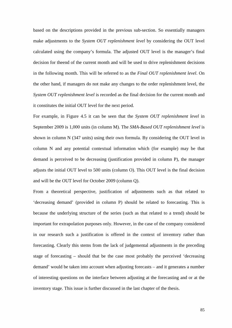
85
based on the descriptions provided in the previous sub-section. So essentially managers
make adjustments to the System OUT replenishment level by considering the OUT level
calculated using the company’s formula. The adjusted OUT level is the manager’s final
decision for theend of the current month and will be used to drive replenishment decisions
in the following month. This will be referred to as the Final OUT replenishment level. On
the other hand, if managers do not make any changes to the order replenishment level, the
System OUT replenishment level is recorded as the final decision for the current month and
it constitutes the initial OUT level for the next period.
For example, in Figure 4.5 it can be seen that the System OUT replenishment level in
September 2009 is 1,000 units (in column M). The SMA-Based OUT replenishment level is
shown in column N (347 units) using their own formula. By considering the OUT level in
column N and any potential contextual information which (for example) may be that
demand is perceived to be decreasing (justification provided in column P), the manager
adjusts the initial OUT level to 500 units (column O). This OUT level is the final decision
and will be the OUT level for October 2009 (column Q).
From a theoretical perspective, justification of adjustments such as that related to
‘decreasing demand’ (provided in column P) should be related to forecasting. This is
because the underlying structure of the series (such as that related to a trend) should be
important for extrapolation purposes only. However, in the case of the company considered
in our research such a justification is offered in the context of inventory rather than
forecasting. Clearly this stems from the lack of judgemental adjustments in the preceding
stage of forecasting – should that be the case most probably the perceived ‘decreasing
demand’ would be taken into account when adjusting forecasts – and it generates a number
of interesting questions on the interface between adjusting at the forecasting and or at the
inventory stage. This issue is further discussed in the last chapter of the thesis.
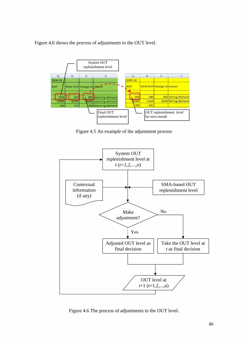
86
Figure 4.6 shows the process of adjustments to the OUT level.
Figure 4.5 An example of the adjustment process
Figure 4.6 The process of adjustments to the OUT level.
System OUT replenishment level
Final OUT replenishment level
OUT replenishment level for next month
System OUT replenishment level at
t (t=1,2,…,n)
SMA-based OUT replenishment level
Make adjustment?
Contextual information
(if any)
Adjusted OUT level as final decision
Take the OUT level at t as final decision
OUT level at t+1 (t=1,2,...,n)
Yes
No
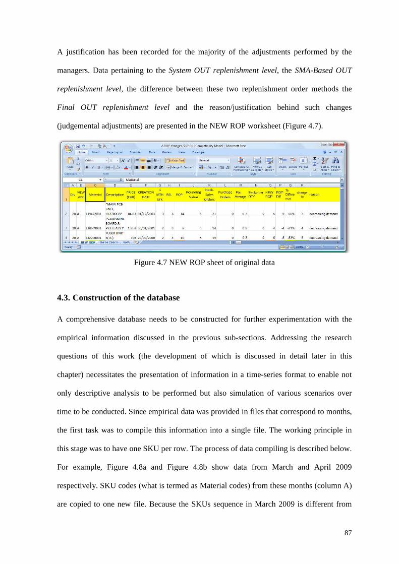
87
A justification has been recorded for the majority of the adjustments performed by the
managers. Data pertaining to the System OUT replenishment level, the SMA-Based OUT
replenishment level, the difference between these two replenishment order methods the
Final OUT replenishment level and the reason/justification behind such changes
(judgemental adjustments) are presented in the NEW ROP worksheet (Figure 4.7).
Figure 4.7 NEW ROP sheet of original data
4.3. Construction of the database
A comprehensive database needs to be constructed for further experimentation with the
empirical information discussed in the previous sub-sections. Addressing the research
questions of this work (the development of which is discussed in detail later in this
chapter) necessitates the presentation of information in a time-series format to enable not
only descriptive analysis to be performed but also simulation of various scenarios over
time to be conducted. Since empirical data was provided in files that correspond to months,
the first task was to compile this information into a single file. The working principle in
this stage was to have one SKU per row. The process of data compiling is described below.
For example, Figure 4.8a and Figure 4.8b show data from March and April 2009
respectively. SKU codes (what is termed as Material codes) from these months (column A)
are copied to one new file. Because the SKUs sequence in March 2009 is different from

88
that in April 2009, we have to make adjustments resulting eventually in one row consisting
of solely one SKU.
Figure 4.8 Compiling information into a time-series format
This process was repeated for all SKUs (materials) and all months and the result can be
seen in Figure 4.9. Column D contains all SKU codes for entire time horizons.
a) b)
c)
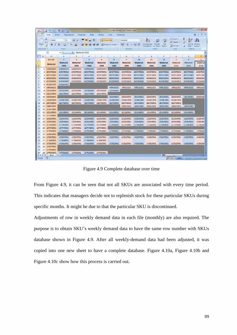
89
Figure 4.9 Complete database over time
From Figure 4.9, it can be seen that not all SKUs are associated with every time period.
This indicates that managers decide not to replenish stock for these particular SKUs during
specific months. It might be due to that the particular SKU is discontinued.
Adjustments of row in weekly demand data in each file (monthly) are also required. The
purpose is to obtain SKU’s weekly demand data to have the same row number with SKUs
database shown in Figure 4.9. After all weekly-demand data had been adjusted, it was
copied into one new sheet to have a complete database. Figure 4.10a, Figure 4.10b and
Figure 4.10c show how this process is carried out.

90
Figure 4.10 Weekly demand data for whole time horizons
The next step in terms of database processing was to establish the detailed OUT-level data
(such as the OUT level resulting from the system, the OUT level calculated by the
company’s formula, the changes to the OUT level made by the manager, and the reasons
for the adjustments). The original data can be seen in Figure 4.11 (an example of data from
March 2009 and April 2009).
b)
c)
a)
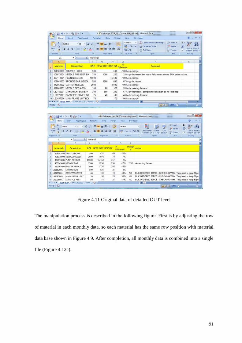
91
Figure 4.11 Original data of detailed OUT level
The manipulation process is described in the following figure. First is by adjusting the row
of material in each monthly data, so each material has the same row position with material
data base shown in Figure 4.9. After completion, all monthly data is combined into a single
file (Figure 4.12c).

92
Figure 4.12 Detailed ROP for whole time horizons
The final step of data handling is to build the complete database, a task that has been
accomplished by deploying Excel Visual Basic for Applications (VBA). The result can be
seen in Figure 4.13.
c)
b)
a)

93
Syntetos et al. (2009b) identified the process of constructing the database needed for
experimentation purposes as a very important one in empirical research. This aspect of
empirical research is generally under-estimated in importance although it arguably
constitutes one of the most important factors towards conducting a comprehensive
experiment. The process of constructing and validating the database used for the purposes
of this research was a very challenging one and particularly demanding in terms of time
investment. Thus it was viewed as necessary to include details here and devote an entire
section to this issue.
Figure 4.13 Complete database for A items
4.4. Detailed research questions
This section develops the main research questions that we attempt to answer through our
empirical investigation. We develop exploratory research questions rather than formal
hypotheses for the following reasons. According to Armstrong (1988), hypothesis testing

94
should be avoided in the scientific research such as the studies in the field of forecasting
since it leads to a lack of an understanding of the final outcomes. Hypothesis testing forces
the researcher to investigate only if something is statistically significant or not rather than
understanding the outcome of the research. In addition, this research follows the
methodological structure of previous research in this field (study conducted by Syntetos et
al., 2009b) where a case is being made for the use of research questions rather than
hypotheses.
Many studies have concluded that managerial interventions in statistical forecasts improve
forecast accuracy (Angus-Leppan and Fatseas, 1986; Lawrence et al., 1986; Mathew and
Diamantopoulos, 1986, 1990, 1992; Diamantopoulos and Mathews, 1989; Wolfe and
Flores, 1990, Syntetos et al., 2009b). Goodwin (2000a) suggested that the use of
judgemental adjustments to statistical forecasts is justified when non-time series
information has predictive power and this information is difficult to capture in a statistical
model. This finding is supported by Goodwin (2005) and Sanders and Ritzman (2001) who
argued that judgement can be valuable when the forecasters have important information
about forthcoming events that is difficult to capture in a statistical model. One would
expect that the benefits of judgemental adjustments that have been reported in the
forecasting literature (the details of which are discussed in Chapter 3) should also apply in
terms of replenishment orders. So it is natural that the first important question that this
research will attempt to answer relates to any potential improvements resulting from
judgementally adjusting stock control decisions. The first research question is the
following:
Q1. Is there any improvement in judgementally adjusting stock control-related
decisions and if so why?

95
Forecasting related research suggests that the size and sign of adjustments have some
explanatory power in terms of performance. When judgemental adjustmentsare integrated
with statistical forecasting, the decision regarding whether a statistical forecast needs
adjusting and the estimate of the size of the adjustment are requirements of the adjustment
process (Lawrence et al., 2006). Some studies (e.g. Fildes et al., 2009) conducted to
investigate the effects of incorporating judgement into statistical forecasts found large
adjustments to be more effective in improving forecast accuracy than small adjustments.
Syntetos et al. (2009b) found that large negative adjustments perform well in improving
forecast accuracy. This knowledge is most useful in terms of potential amendments to FSS.
In order to improve the effectiveness of FSS functions, Lee et al. (2007) reported an
experiment that investigated the effectiveness of providing support for the use of analogies
in sales forecasting. (By analogies we mean the similarity of conditions between past and
forthcoming events; thus the environment of these conditions is relatively predictable, for
example the environment of similar promotion campaigns.) This study argued that by
providing contextual information of similar events, forecasters are supported in their
efforts to determine how much they should adjust statistical sales forecasts. These studies
indicate that the performance of judgemental forecasting may be increased by knowing the
implications of the sign and size of adjustments. This benefit may also be found in an
inventory context. We may expect that the performance of a stock control system can be
improved by analysing the behaviour of human intervention in inventory decisions in terms
of the sign and size of adjustments and their effect for improving the inventory
performance. Accordingly, the second research question of this study is:
Q2. How the sign and size of the adjustments affects the performance of
inventory system?

96
Documentation of reasons that a particular forecasting model is chosen and why
adjustments of forecasts are made is important in reducing bias in relevant processes
(Goodwin, 2000). Such documented reasons could be used in determining why a forecast
is potentially erroneous since the rationale of decision making on the part of the forecaster
is recorded and can be evaluated. In addition, models of the forecaster’s behaviour should
explain when and how individuals incorporate judgement into their predictions (Stekler,
2007). In the area of judgementally adjusted stock control decisions, it seems that
providing justification for adjustments may be associated with an improved performance of
the stock control system. This research uses data where the justification for adjustments is
available in the majority of cases. An evaluation is conducted to assess whether offering a
justification for the adjustments seems to improve the performance of the inventory
system. This analysis constitutes a major contribution to the inventory literature since no
research has covered similar aspects before. The third research question of this study is:
Q3. Is any improvement achieved by the adjustments for which justification is
offered as compared to those without a justification and if so why?
In statistics, bias is defined as the characteristic of an experimental or sampling design that
systematically (non-randomly) affects the results of a study (Evans, 1992). In this research,
we can say that bias is a systemic inaccuracy due to the characteristics of the process
employed in making adjustments to replenishment orders. Tversky and Kahneman (1974)
argued that by making judgemental adjustments, people assessing probabilities and
predicting values are using heuristic principles. The researchers argued that, sometimes,
heuristic principles have systemic errors; thus they concluded that biases are found in the
intuitive judgement of probability. Moreover, Carter et al. (2007) argued that from a
managerial standpoint, understanding the nature of decision biases is the first step in the
process of deciding how to manage them. These authors also developed a taxonomy of

97
judgement and decision-making biases which can impact supply management decision-
making, such as availability cognition, base rate, presentation, and control illusion.
In the field of forecasting, many studies have investigated the issue of bias in
judgementally adjusting forecasts (see, for example, Diamantopoulos and Mathews, 1989;
Matthews and Diamantopoulos, 1990; Goodwin and Wright, 1994) as forecasters operate
in an environment where there are either implicit or explicit biases (Lawrence and
O’Connor, 2005). Forecasters may adjust forecast results for a particular reason, and there
are clearly two directions in which bias may occur resulting in either under- and over-
forecasting. For example, a manager may increase a statistical forecast to achieve a sales
target or to get priority from a supplier or conversely may decrease a forecast if for
example inventory cost reductions drive current operations. Biased/unbiased judgementally
adjusted forecasting affects the accuracy of its results. The relationship between the
forecaster’s characteristics and forecasting performance is evaluated by Eroglu and
Croxton (2010). This research considers a number of types of bias (optimism bias,
anchoring bias, and over-reaction bias) to explore the effects of particular individual
differences (personality, motivational orientation, and work locus of control) on
forecasting performance. The researchers found that a forecaster’s personality and
motivational orientation have significant effects on forecasting bias, whereas work locus of
control does not. As judgemental forecasting introduces bias and the effects of bias impact
on the performance of forecasting, it seems possible that bias can also be found in the
process of inventory decision making. By analysing whether a judgmentally adjusted stock
control decision is biased or not, further analysis may be conducted in order to investigate
how and why managers made adjustments. Therefore, this research investigates the biases
in inventory decision making and this aspect forms the fourth of the research questions:
Q4. Are judgementally adjusted stock control decisions biased?

98
Although the phenomena of learning and forgetting occurs in manufacturing systems
(Towill, 1990; Alamri and Balkhi, 2007) and many learning models have already been
developed (see section 3.9) there is some evidence that there is no learning effect in the
forecasting function (Syntetos et al., 2009b). Klassen and Flores (2001) showed that there
is no learning perspective from the organisation or from individual forecasters over time.
Moreover, when examined the way of people to utilize contextual information in
conjuction with time series to produce a forecast, Lim and O’Connor (1996) found that
people did not seem to learn over time to modify their behavior when adjusting statistical
forecasts. The findings above is supported by Nikolopoulos et al. (2006) when isvestigated
an organisational and individual learning perspective within the organisation. This study
reported the gaps in the learning loop within the company as there is no performance
improvement over time of forecasting resulted by software system as well as the
judgementally adjusted forecasts. On the other hand, Lee et al. (2007) suggested that
forecasters often use information from analogous events from the past to help to estimate
the effect of an anticipated special event. In terms of improving the performance of
judgemental adjustments, Bolger and Wright (1994) interpreted the pattern of performance
in terms of ecological validity and learnability. Ecological validity is the degree to which
experts are required to make judgements inside or outside the domain of their professional
experience. Learnability is the degree to which good judgement can be learned in a
domain-related task. It is obvious that learning effects occurs in most inventory system
since this system contain repetitive processes and incorporated human intervention in
making stock control decision. Our study attempt to investigate this issue as the
performance of inventory system may be improved by recognising the behaviour of

99
manager in making adjustments on replenishment order decisions. Thus, the next research
question is:
Q5. Is there any learning taking place in the process of adjusting stock control
quantities and if so how?
In the forecasting area, it has been shown that combining the forecasts produced by
different methods may lead to a performance that is better than that of the individual
forecasts themselves (Makridakis and Hibon, 1979). The case study organisation
implemented three replenishment order methods: System OUT replenishment level, the
SMA-Based OUT replenishment level, and the Final OUT replenishment level. By
combining these methods, it is reasonable to expect that the performance of the inventory
system (service level, fill rate, and cost) may improve as compared to that resulting from
the replenishment suggestions of a single method. Accordingly, our sixth research question
is:
Q6. What is the effect of combining methods on the calculation of the OUT level?
Many organisations implement the SMA forecasting method because it is simple to use
and is familiar to managers (Boylan and Johnston, 2003). The case study organisation
employs SMA forecasting to calculate the SMA-based OUT replenishment level which in
turns is taken into account (jointly with any external information) to adjust System OUT
replenishment level. Hence, it will be interesting to discover the relationship between the
SMA-based OUT replenishment level and the Final OUT replenishment level, and whether
the influence of the former to the latter is statistically significant. Thus, the next research
question is:
Q7. What is the explanatory power of the SMA-Based OUT replenishment level on
the Final OUT replenishment level?

100
4.5. Research classification
According to Collis and Hussey (2009), research can be classified into four types,
according to its purpose, its process, its logic and its outcome. The purpose of the research
relates to the reason why it is conducted, while the process relates to the way in which the
data were collected and analysed. The logic of the research involves the decision whether
the research moves from the general to the specific or vice versa, and the outcome may be
either the solution to a particular problem or a general contribution to knowledge. Table
4.1 presents the classification of research.
Table 4.1 Classification of main types of research
No Basis of classification Type of research 1 Purpose of the research Exploratory, descriptive, analytical, or predictive research 2 Process of the research Quantitative or qualitative research 3 Logic of the research Deductive or inductive research 4 Outcome of the research Applied or basic research
(source: Collis and Hussey, 2009, pp. 4)
Exploratory research is conducted when there are few or no earlier studies on the topic
(Collis and Hussy, 2009). Cooper and Schindler (2002) add that exploratory study is useful
when possible problems that might arise during the study are not clearly identified.
Accordingly, the current study is exploratory in nature because the availability of literature
on the phenomenon being investigated is very limited. Further, as far as we know, this
study is the first to investigate the effects of human intervention on stock control decisions.
The process and logic of the research involve quantitative and semi-deductive research
respectively. Details of the research process (or research choice) can be found in sub-
section 4.6.4 and of the research logic (research approach) in sub-section 4.6.2.
By its outcome, this is applied research since the findings resulting from empirical data
analysis are expected to solve a particular problem in inventory systems, and to improve
management practice and policy in this area.

101
4.6. Research methodology
The description of the research methodology employed here follows the ‘Research Union’
conceptual framework proposed by Saunders et al. (2009). This approach enables a clear
definition of any research process from the underlying philosophical considerations to the
data collection and analysis methods. Before we introduce the various concepts underlying
this research, an outline of the exact sequence of activities performed will better link the
forthcoming discussion to the research itself.
Following a critical review of the literature, a number of research questions were
developed to provide guidelines as to what sort of adjustments practitioners tend to
perform. These might relate to their size, frequency, sign (positive or negative), and when
the adjustments are performed. A link may be made to the underlying demand pattern and
data characteristics; for example, people tend to adjust forecasts when demand is
repeatedly high. An empirical database was then constructed to facilitate exploration of the
extent to which the theoretical claims based on previous research might be sustained. This
empirical database contained actual demand information, statistical forecasts, statistically-
derived system replenishment decisions and judgementally adjusted replenishment
decisions (and in many cases the adjustments were accompanied by a justification). As
such, it enabled an exploratory analysis as well as simulating the effects of judgemental
adjustments (using Visual Basic embedded in Excel).
After collection of all the information, the research questions are revisited and tangible
suggestions made to practitioners. We will elaborate on the process discussed above later
in this section, with a detailed diagram that presents the research.
4.6.1. Research philosophy
The research philosophy relates to the development of knowledge and the nature of that
knowledge and contains important assumptions about the way we see the world (Saunders

102
et. al., 2009). There are three major ways of thinking about research philosophy:
epistemology, ontology and axiology (Saunders et al., 2009) and each philosophy can be
seen as a continuum.
Epistemology is concerned with the study of knowledge and what we accept as being
valid, in other words, examination of the relationship between the researcher and what is
being researched (Collis and Hussey, 2009) or the relationship between the researcher and
the participant (Teddlie and Tashakkori, 2009). Some scholars name the spectrum of
epistemology differently, but the meanings are the same. Saunders et al. (2009) define the
extremes of the spectrum of epistemology as positivism and interpretivism; Easterby-Smith
et al. (2004) use the terms positivism and social constructivism, while Collis and Hussey
(2009) refer to it as positivism and phenomenology.
Positivism is the epistemological position where the social world exists externally; it holds
that its properties should be measured through objective methods (Easterby-Smith et al.,
2004). Bryman and Bell (2011) and Denscombe (2010) relate positivism to the application
of methods from natural science to the social sciences. On the other hand, interpretivism
attempts to minimise the distance between the researcher and what is being researched
(Collis and Hussey, 2009).
The current research aims to explore the effects of incorporating human judgement into
inventory decision making. Data gathering involves the simulation results of the
performance of judgemental adjustments in a real-world context. The focus is on the effect
of those adjustments (analysis to be performed via simulation) which emphasises
generalisation (although arguably such generalization may not be achievable). Hence, the
epistemological assumptions of this research lie at the positivism pole.
Ontology relates to assumptions about the nature of reality (Collis and Hussey, 2009;
Easterby-Smith et al., 2004 and Saunders et al., 2009). The ontology continuum spans

103
objectivism to subjectivism. Objectivism assumes that social entities exist in reality
externally to social actors, while subjectivism supports the notion that social phenomena
stem from the perceptions and consequent actions of social actors (Saunders et al., 2009).
Lincoln and Guba (1985) add that positivists believe that there is a single reality, while the
constructivist or interpretivist defines reality as multiple. This research relies upon an
objective (yet not necessarily generalisable) outcome of simulation analysis, so it is clear
that on the ontological continuum objectivism is favoured.
Axiology is a branch of philosophy that studies the judgements being made about ‘values’
(Saunders et al., 2009). It is a continuum on which an assumption has to be made as to
whether the research is ‘value free’ and unbiased or ‘value laden’ and biased (Collis and
Hussey, 2009). As this research involves the quantitative output of well-structured
simulation experiments (where the findings are, or the intention at least is to produce
findings that are, unbiased), our axiological assumptions lie at the ‘value free’ pole.
Following this explanation of the differences between the three philosophies, Table 4.2
summarises the difference between positivist and interpretivist approaches in general
(Lincoln and Guba, 1985), and Figure 4.14 depicts the philosophical positioning of this
research.
Table 4.2 Contrasting positivist and interpretivist
Axioms about Positivist paradigm Naturalist (constructivist/ interpretivist) paradigm
Ontology: the nature of reality
Reality is single, tangible, and fragmentable
Realities are multiple, constructed, and holistic
Epistemology: the relationship of knower to the known
Knower and known are independent, a dualism
Knower and known are interactive, inseparable
Axiology: the role of values
Inquiry is value-free Inquiry is value-bond
(source: Lincoln and Guba, 1985, pp. 8)
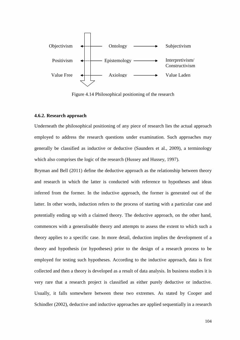
104
Figure 4.14 Philosophical positioning of the research
4.6.2. Research approach
Underneath the philosophical positioning of any piece of research lies the actual approach
employed to address the research questions under examination. Such approaches may
generally be classified as inductive or deductive (Saunders et al., 2009), a terminology
which also comprises the logic of the research (Hussey and Hussey, 1997).
Bryman and Bell (2011) define the deductive approach as the relationship between theory
and research in which the latter is conducted with reference to hypotheses and ideas
inferred from the former. In the inductive approach, the former is generated out of the
latter. In other words, induction refers to the process of starting with a particular case and
potentially ending up with a claimed theory. The deductive approach, on the other hand,
commences with a generalisable theory and attempts to assess the extent to which such a
theory applies to a specific case. In more detail, deduction implies the development of a
theory and hypothesis (or hypotheses) prior to the design of a research process to be
employed for testing such hypotheses. According to the inductive approach, data is first
collected and then a theory is developed as a result of data analysis. In business studies it is
very rare that a research project is classified as either purely deductive or inductive.
Usually, it falls somewhere between these two extremes. As stated by Cooper and
Schindler (2002), deductive and inductive approaches are applied sequentially in a research
Subjectivism Objectivism
Interpretivism/Constructivism
Positivism
Value Laden Value Free
Ontology
Epistemology
Axiology

105
project and can be combined. For example, the hypothesis is developed to explain the
phenomenon in question, then a study is designed to test the hypothesis. In addition,
Remenyi et al. (1998) argue that the relation between data and theory is complex and it is
difficult to clearly justify which comes first. They explain that it is impossible to generate
theory without data, but on the other hand data cannot be collected without a theoretical
framework. In other words, we may say that both deductive and inductive approaches are
commonly deployed together in management research to achieve the research objective.
Our approach may be characterised as semi-deductive; it is outlined in Figure 4.15 and
then presented in more detail in Figure 4.16.
Deductive Approach Inductive Approach
Test Develop
This Research: integrated
Investigate Further Information
Figure 4.15An integrated (semi-deductive) research approach
First, we develop research questions based on the literature review. Since judgementally
adjusted stock control decision theory is rare, we cite the underpinning theory of
judgmental forecasting instead. This is valid because stock control and forecasting in
Theory Empirical Data
Theory Empirical Data
Theory
Empirical Data

106
inventory systems are closely related. Development of the research questions means that
we are implementing the inductive approach.
Figure 4.16 The research approach in detail
Furthermore, the exploratory analysis of the constructed empirical database addresses the
research questions by conducting a simulation experiment. The simulation process, which
will produce the findings of the research, is the deductive part. Finally, we use the findings
to generate some conclusions; this means that we introduce knowledge to the theory from
the data, a process which is clearly inductive.
INDUCTIVE
INDUCTIVE
DEDUCTIVE
Conduct literature review
Develop research questions
Analyse empirical data
Conclusions
Construct empirical database
Recommendations
Findings

107
4.6.3. Research strategy
A research strategy constitutes a general plan of how the researcher will go about
answering the research questions (Saunders et al., 2009). There are many types of research
strategies and various scholars classify them in different ways. For example, Saunders et
al. (2009) refer to experiments, surveys, case studies, action research, grounded theory,
ethnography and archival research. Bryman (2008) defines a research strategy as a research
design which consists of five types: experimental design, cross-sectional or survey design,
longitudinal design, case study design, and comparative design. Yin (2009) defines it as a
method which can be placed into five categories: experiment, survey, archival analysis,
history and case study. In addition, according to Yin (op.cit.), in choosing a research
strategy there are three conditions to be considered: the type of research question, the
extent of control an investigator has over actual behavioural events and the degree of focus
on contemporary as opposed to historical events. Table 4.3 displays these conditions and
their relation to research strategy.
Table 4.3 Relevant situations for different research methods
Method Form of Research Question
Requires Control of Behavioural Events?
Focuses on Contemporary Events?
Experiment How, Why? Yes Yes
Survey Who, What, Where, How Many, How Much? No Yes
Archival Analysis
Who, What, Where, How Many, How Much? No Yes/No
History How, Why? No No Case Study How, Why? No Yes
(source: Yin, 2009, pp. 8)
This research investigates contemporary events: the process of judgementally adjusting
stock control decisions. The research involves a number of control parameters, upon which
the performance of the inventory system is dependent and essentially sensitivity analysis is
conducted to reach conclusions. As discussed by Cooper and Schindler (2002), if a
researcher intends to investigate the effect of certain variables on other variables then the

108
experimental method is appropriate. Further, this research involves the ‘how’ and ‘why’
questions as generated in section 4.4. These are answered by experiment and statistical
analysis. Based on the above discussion, it is clear that the most suitable research strategy
for this study is experiment.
4.6.4. Research choice
Saunders et al. (2009) use the term ‘research choice’ to distinguish the options available
for data collection and data analysis. In general, the options are whether to use the
qualitative method, quantitative method, or a combination of the two (Figure 4.17). Collis
and Hussey (2009) refer to qualitative data as data in nominal form, and quantitative data
as data in numerical form. The research that combines both the qualitative and quantitative
methods is referred to as ‘mixed method’ (Teddlie and Tashakkori, 2009). Table 4.4
presents the differences in these three research choices.
Figure 4.17 Research choices (source: Saunders et al., 2009, pp. 152)

109
Table 4.4 Dimension of contrast among the three research choices
Dimension of contrast
Qualitative Position Mixed Method Position Quantitative Position
Methods Qualitative methods Mixed methods Quantitative methods Researchers QUALs Mixed methodologists QUANs Paradigms Constructivism (and
variants) Pragmatism; transformative perspective
Postpositivism Positivism
Research questions
QUAL research questions MM research questions (QUAN plus QUAL)
QUAN research questions; research hypothesis
Form of data Typically narrative Narrative plus numeric Typically numeric Purpose of research
(Often) explanatory plus confirmatory
Confirmatory plus exploratory
(Often) confirmatory plus exploratory
Role of theory; logic
Grounded theory; inductive logic
Both inductive and deductive logic; inductive-deductive research style
Rooted in conceptual framework or theory; hypothetico-deductive model
Typical studies or designs
Ethnographic research designs and others (case study)
MM designs, such as parallel and sequential
Correlational; survey; experimental; quasi-experimental
Sampling Mostly purposive Probability, purposive, and mixed
Mostly probability
Data analysis Thematic strategies: categorical and contextualizing
Integration of thematic and statistical; data conversion
Statistical analyses; descriptive and inferential
Validity/trust worthiness issues
Trustworthiness; credibility; transferability
Inference quality; inference transferability
Internal validity; external validity
(source: Teddlie and Tashakkori, 2009, pp. 22)
Accordingly, in line with its research paradigm and in order to achieve the research
objectives, this research adopts a single method approach, which is the quantitative
approach. Data is in numerical form and is analysed using statistical methods.
4.6.5. Time horizons
The ‘time horizon’ is a term employed to analyse whether the research investigation
focuses on one particular time or over a period of time. Saunders et al. (2009) describe the
first as cross-sectional and the second as longitudinal study. In cross-sectional studies, the
researcher examines one particular phenomenon at a particular time, whereas in
longitudinal studies he/she examines changes in phenomena over a period of time.
This study does not intend to investigate changes in the phenomenon being analysed over
time, or compare how the phenomenon changes from one particular time to another. Thus,
the time horizon of the research is cross-sectional.

110
4.6.6. Research techniques
Research techniques refer to the method of collecting data and the procedures for analysis.
In general, as the research strategy is experiment, data is gathered from one organisation
that has relevant experience in judgemental adjustments, and more specifically from a
company that can meet the aims and objectives of this research.
The quantitative information to be used for this study relates to an empirical database that
contains, in a time-series fashion, historical demand information, statistical (system)
forecasts, statistical (system) replenishment decisions and the judgemental adjustments
superimposed on the system replenishments leading to the final replenishment decisions.
Simulation may then be performed in order to evaluate in a dynamic fashion the added
value (if any) of employing judgement. Details of the simulation process are presented in
section 5.5. Using the database, we will be able to relate performance to the underlying
demand characteristics, enabling us to provide an answer as to when adjustments are
beneficial.
4.7. Conclusions
This research uses the data from an organisation representing the European Logistics head
office of a Japanese electronics manufacturer. This organisation has implemented an ERP
package, SAP R/3. This software is used to define the initial value of replenishment order
decisions before it is adjusted by the managers based on external information. Empirical
data from this case organisation and the process of adjustment of the order-up-to (OUT)
levels was explained, followed by the construction of a database to facilitate empirical
analysis through simulation. Finally, the research questions were formulated based on the
literature review. These research questions will be addressed through the empirical data
analysis presented in Chapter 5.

111
In this chapter we also discussed the research methodology followed in this work. The
research paradigm of this study lies at the positivist end of the spectrum. It employs
experiment as the research strategy and quantitative methods as the research choice.
Figure 4.18 summarises the methodological approach used in this study.
Figure 4.18 The research onion of this work
(source: Saunders et al., 2009, pp. 108)
Quantitative
Research Philosophy
Research Approach
Research Strategy
Research Choice
Time Horizon
Data Collection and
analysis
Positivism
Semi-deductive
Simulation and Experimentation
Mono method
Short- term

112
Chapter 5. EMPIRICAL DATA ANALYSIS AND FINDINGS
This chapter describes the analysis of the Stock Keeping Units (SKUs) available for the
purposes of this research (in terms of the demand data, prices etc), the judgemental
adjustments performed to the Order-Up-To (OUT) levels and the justification provided by
managers when performing adjustments. Analysis is also conducted, partly through
simulation, to answer the research questions developed in the previous chapter.
The data was gathered from June 2009 to August 2011. In total, 359 A-class and 1,454 B-
class SKUs are considered for the purposes of this research. The total number of SKUs
appearance for the whole period was 4,661 times for A-class and 15,365 times for B-class.
Since managers do not necessarily make adjustments (or provide justifications when they
do so) for each and every period related OUT level, relevant data is extracted depending on
the task (research questions addressed) out of the total database and analysed accordingly.
Accordingly, adjustment of OUT level was made 1,461 and 2,958 times for A-class and B-
class respectively.
5.1. Demand descriptive statistics
First, it is viewed as imperative to develop an understanding on the nature of the demand
and its characteristics. Demand per period, demand sizes, and inter-demand intervals are
considered for that purpose. The demand data characteristics are summarised in Table
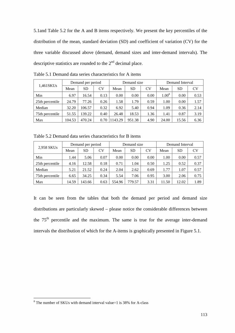
113
5.1and Table 5.2 for the A and B items respectively. We present the key percentiles of the
distribution of the mean, standard deviation (SD) and coefficient of variation (CV) for the
three variable discussed above (demand, demand sizes and inter-demand intervals). The
descriptive statistics are rounded to the 2nd decimal place.
Table 5.1 Demand data series characteristics for A items
1,461SKUs Demand per period Demand size Demand Interval
Mean SD CV Mean SD CV Mean SD CV
Min 6.97 16.54 0.13 0.00 0.00 0.00 1.008 0.00 0.53
25th percentile 24.79 77.26 0.26 1.58 1.79 0.59 1.00 0.00 1.57
Median 32.20 106.57 0.32 6.92 5.40 0.94 1.09 0.36 2.14
75th percentile 51.55 139.22 0.40 26.48 18.53 1.36 1.41 0.87 3.19
Max 104.53 470.24 0.70 1143.29 951.38 4.90 24.00 15.56 6.36
Table 5.2 Demand data series characteristics for B items
2,958 SKUs Demand per period Demand size Demand Interval
Mean SD CV Mean SD CV Mean SD CV
Min 1.44 5.06 0.07 0.00 0.00 0.00 1.00 0.00 0.57
25th percentile 4.16 12.58 0.18 0.71 1.04 0.50 1.25 0.52 0.37
Median 5.21 21.52 0.24 2.04 2.62 0.69 1.77 1.07 0.57
75th percentile 6.65 34.25 0.34 5.54 7.06 0.95 3.00 2.06 0.75
Max 14.59 143.66 0.63 554.96 779.57 3.31 11.50 12.02 1.89
It can be seen from the tables that both the demand per period and demand size
distributions are particularly skewed – please notice the considerable differences between
the 75th percentile and the maximum. The same is true for the average inter-demand
intervals the distribution of which for the A-items is graphically presented in Figure 5.1.
8 The number of SKUs with demand interval value=1 is 38% for A-class

114
Figure 5.1 The distribution of average inter-demand interval for A items.
Intermittent demand (and demand size/inter-demand interval) distributions are indeed
known to be very skewed and previous empirical studies have confirmed such a fact
(Syntetos et al., 2009b, 2010a, 2010b; Teunter et al., 2010; Nikolopoulos et al., 2011). For
a summary of arguments on this issue of statistical distributions in an intermittent demand
context please refer to Syntetos et al. (2012). As expected the demand sizes for the A items
appear to be (considerably) higher than those related to the B items whereas the inverse is
true with regards to the inter-demand intervals.
5.2. Price of the SKUs
Information related to SKU prices9 has been made available to us by the company. There
are 359 and 1,454 SKUs for A and B items respectively. The price varies between €0.02
9 Please note that those are final selling prices as opposed to cost information that is typically available in empirical studies. We argue that profit margins are relatively constant in a service parts context rendering prices differing from cost by a constant amount across all SKUs. This is important when we analyse inventory costs and implications since inventory theory has been built upon item costs, and inventory holding costs are calculated taking into account the cost of an items not its price.

115
and €254.85 for A items and €0.02 and €425.44 for B items. Table 5.3 shows the range of
service10 parts prices for the A and B items.
Table 5.3 Spare parts prices for A items and B items.
Description A items (€) B items (€) Min 0.02 0.02 25th percentile 5.69 0.87 Median 19.09 4.09 75th percentile 35.67 18.12 Max 254.85 425.44
It can be seen from Table 5.3 that the range of prices for the B items is wider than that
related to the A items with the maximum price being almost twice as big. The price of
material is an important factor to be considered since the case organisation carried out the
SKUs classification based on demand value (volume × price). In this classification method,
SKUs are distinguised based on their value or benefit to the organisation, as a result the
items that have more value get more attention from manager.
Regarding the judgemental adjustments performed by managers on the OUT levels it
seems that they have not been taking into account the price of the relevant SKUs when
coducting such adjustemnets. This can be seen from the justification asscociated with
them. Most of the reasons provided for adjusting the OUT levels are merely related to the
demand for spare parts (or in fact the perceived demand for spare parts), their inventory
position, and/or replenishment orders related information, but not the SKU prices. We
return to this issue in section 5.4, where the justifications of judgemental interventions are
discussed.
There are a number of studies commenting on the importance of cost analysis in an
inventory control context. Teunter et al. (2010) proposed a new cost criterion for ranking
SKUs which takes criticality of SKUs into account through the shortage cost. In most
practical situations, the measurement of criticality is based on the rate of demand value
10 The words ‘service’ and ‘spare’ parts are used interchangeably in this research.

116
(price multiplied by demand volume) or the demand volume for an SKU or the functioning
of a spare part of equipment in the service/maintenance industries. By conducting
experiments using three real-life datasets, it was found that the cost criterion outperformed
the traditional demand value and demand volume criteria and also a criterion proposed by
Zhang et al. in 2001 for minimising the safety stock cost. The results indicate the inventory
cost reductions resulting from employing the new approach with no penalty in the
customer service level achieved. Syntetos et al. (2009a) proposed a modified periodic
OUT-level policy that relies on inter-demand intervals and demand sizes, when demand
occurred. This policy is employed in a simulation experiment using actual lead-times and
unit cost information. The results indicate the inventory cost reduction resulting from the
employment of the new approach. In another study, Syntetos et al. (2010b) explored
forecasting- and stock control-related opportunities for increasing service levels and
reducing costs in the wholesale context. There are still no studies that discuss the relation
between cost and judgementally adjusted stock control decisions.
Figure 5.2 and Figure 5.3 present the distribution of the SKU prices for the A and B items
respectively.

117
Figure 5.2 Distribution of material price for A items
768
149
11492
119
4528 22
624
9 9 4 5 7 2 3 4 8 4 1 3 2 5 1 3 1 2 1 1 1 0 0 1 1 0 1 1 0 2 0 0 0 1 0 1 2 0 1
0
100
200
300
400
500
600
700
800
Fre
qu
en
cy
Material Price
Figure 5.3 Distribution of material price for B items
It can be seen (as already discussed in Table 5.3) that B items are associated with a higher
cost (price). However, B items have been also shown to be (by the very definition of the
ABC classification performed by the company) more intermittent in nature, resulting
118
presumably in higher obsolescence and having a much greater impact on stock stock-
holding costs. Although A items are ‘officially’ defined as more important in terms of
frequency of occurring, B items may in fact require more attention from managers with
regards to stock control. These findings are in line with the theories reviewed in Chapter 2.
5.3. Analysis of judgemental adjustments
In this section we conduct an analysis of the adjustments performed on the initial-OUT
level in every inventory period. Correspondingly, the magnitude of the adjustments (and
their sign) may be calculated by observing the difference between two consecutive Final
OUT replenishment levels. Please recall, that the initial OUT level in each period is
judgementally adjusted (taking also into account the SMA-based OUT replenishment
level) and that results into the Final OUT replenishment level (that is used for stock control
purposes) that is used as the initial one in the next time period.
Adjustments are assessed and analysed in terms of the distribution of their signed size,
absolute size, relative signed sizeand relative absolute size, to capture collectively the
characteristics of both magnitute and direction (both in absolute and relative terms, the
latter relating to the level of the demand). The relative signed size and absolute size are
calculated by divided the difference between successor and predecessor Final OUT
replenishment levels over the predecessor Final OUT replenishment level. The goodness-
of-fit of various plausible theoretical statistical distributions is analysed using the
Kolmogorov-Smirnov (K-S) test. The K-S test is chosen since there is no requirement for
grouping the data into categories, which is limiting requirement associated for example
with the Chi-Square test. When applying the Chi-Square test, the data needs to be grouped
into categories to ensure that each is associated with an expected frequency of a minimum
of a certain number of observations (Syntetos et al., 2012; Lengu, 2012). Since the demand

119
nature of data used in this study is intermittent, consequently the adjustment data is also
intermittent, it would be difficult to meet the minimum and average expected frequencies
of the categories. Moreover, the critical values used in the K-S goodness-of-fit test are
independent of the hypothesised distribution. This means that the test does not rely on
assumptions that the data is drawn from a particular probability distribution. Thus, the
computation required when using the K-S test is simple and less time-consuming.
However, the K-S test assumes continuous distributional functions, which is not in
accordance with the random variables to be tested (adjustments). This is a major drawback
although we would very much like anyway to consider continuous distributions due to the
fact that they are generally more flexible than discrete distributions and they do provide
good approximations. For a summary of arguments in favour of the K-S test the interested
reader is referred to Lengu (2012).
We consider distributions with no more than 2 parameters. The number of parameters is
limited to two to reflect a trade-off between goodness-of-fit and computational
requirements. Single or two-parameter distributions are easier to handle and in an
inventory control context they constitute the norm. The goodness-of-fit tests are conducted
by deploying the EasyFit Software. There are nine theoretical distributions that have been
considered, for both the absolute and signed cases analysed. In the former case,
distributions defined only in the positive domain have been considered. These distributions
are shown in Table 5.4. The critical values have been computed based on K-S statistical
tables for 1% and 5% significant levels. We consider that: i) there is a ‘strong fit’ if the P-
value is less than the critical value for 5%; ii) there is ‘good fit’ if the P-value is less than
the critical value of 1% but larger than that for 5%; and iii) there is a ‘no fit’ if the P-value
is larger than the critical value for 1%.

120
Table 5.4 Theoretical distributions being tested
No. Absolute size and relative absolute size adjustments
Signed size and relative signed size adjustments
1 Cauchy Cauchy 2 Exponential Error function 3 Gamma Gumbel max 4 Gumbel max Gumbel min 5 Gumbel min Logistic 6 Logistic Normal 7 Normal Uniform 8 Uniform Hypersecant 9 Weibull Laplace
5.3.1. Goodness-of-fit tests and distributional considerations
Considering that managers have not been performing adjustments in every period for each
SKU, we end up with 1,461 (31.35%) and 2,958 (19.25%) adjustments for the A and B
items respectively. The goodness of fit tests indicate that none of the distributions provide
a strong fit when all the adjustments are considered collectively across the two classes of
items. That is, we have first attempted to assess a potential goodness of fit on all the
adjustments performed in the A and B items (separately for each category). This was partly
expected since adjustments should relate closely to the characteristics of a particular SKU.
However, we did wish to check for any ‘universal’ conclusions. The results indicate that
adjustments have to be considered separately for each SKU and we return to this issue later
in this sub-section. The detailed results of the goodness-of-fit testsdiscussed above are
shown in Appendix Eand the summary of the best fitting distributions can be seen in Table
5.5.

121
The distribution of the signed size of adjustments, absolute size of adjustments, relative
signed size and relative absolute size and the fitted distributions for the A items are
indicated in Figure 5.4, Figure 5.5, Figure 5.6, and Figure 5.7, respectively. For all
distribution graphs, the horizontal axis (x) represents the interval of adjustment data and
the vertical axis (f(x)) represents the probability density function (PDF) of the theoretical
distribution (please see Table 5.5 for the best fitting distribution) and the number of
adjustments in the corresponding interval.
Figure 5.4 Distribution of the signed size of adjustments for A items

122
Figure 5.5 Distribution of the absolute size of adjustments for A items
Figure 5.6 Distribution of the relative signed size of adjustments for A items

123
Figure 5.7 Distribution of the relative absolute size of adjustments for A items
Figure 5.4 indicates that most decisions made by the managers related to decreasing the
OUT level up to 20 units (29.23% of total decisions). For the absolute size of adjustments,
it was similarly found that those are associated with a mode interval of [0 – 20] units
(Figure 5.5).Relatively small adjustments are known to be very popular in the forecasting
domain representing mostly reaction to noise or a need on the part of the forecaster (stock
controller in this case) for a sense of ownership of the process. However, a qualification of
‘small’ is required here that may not be perceivable unless a ‘relative’ analysis is
performed.
Figure 5.6 and Figure 5.7 show the relative signed size and relative absolute size of
adjustments. There are two considerable spikes in the former case, where the mass function
though is indeed concentrated in the centre. On the other hand, the relative absolute size of
adjustments seems to peak at [20% – 25%]. The above analysis, confirms previous results
in the forecasting literature on the prevalence of relatively small adjustments.

124
The distribution of the signed size of adjustments, absolute size of adjustments, relative
signed size and relative absolute size of B items is shown in Figure 5.8, Figure 5.9, Figure
5.10, and Figure 5.11 respectively.
Figure 5.8 Distribution of the signed size of adjustments for B items
Figure 5.9 Distribution of the absolute size of adjustments for B items

125
Figure 5.10 Distribution of the relative signed size of adjustments for B items
Figure 5.11 Distribution of the relative absolute size of adjustments for B items
Figure 5.8 shows that the most frequent decisions made by the manager are to increase the
OUT level by 0 – 10 units; these constitute nearly 20% of all decisions. In line with this,
the absolute size of adjustments also indicates that 1,175 (39.72%) of decisions are to
increase/reduce the OUT level within the range of [0–10] units.

126
In relative terms, and similar to the patterns identified for the A items, the distribution of
the relative signed adjustments in B items is associated with two spikes. The peak related
to negative and positive adjustments occurs at the [-30% – -35%] (261 judgements) and
[35% –40%] (189 judgements) interval respectively. The relative absolute size of the
adjustments is [30% and 35%]. It seems that greater adjustments are performed for the B
items rather than A and this may be related to the greater eventual importance of such
items from a stock control perspective (both in terms of obsolescence and stock holding
costs) discussed earlier in this chapter. The above analysis is summarised in Table 5.5
where the best fitting distributions for each case is also indicated.
Table 5.5 Adjustment distributions for A items and B items.
A items B items Signed size of adjustment
• Most adjustments are between 0 – -20 units
• Cauchy distribution
• Most adjustments are between 0 – 10 units
• Weibull distribution Absolute size of adjustment
• Most adjustments are between 0 – 20 units
• Gamma distribution
• Most adjustments are between 0 – 10 units
• Gamma distribution Relative signed size of adjustment
• Most adjustments are between -25% – -30% (negative adjustments) and 5% – 15% (positive adjustments)
• Cauchy distribution
• Most adjustments are between -30% – -35% (negative adjustments) and 35% –40% (positive adjustments)
• Cauchy distribution Relative absolute size of adjustment
• Most adjustments are between 20% – 25%
• Gamma distribution
• Most adjustments are between 30% – 35%
• Cauchy distribution
Returning to the issue of the goodness of fit, since there is no single theoretical distribution
(from those assessed in this study at least) that fits (strongly) the adjustments when those
are considered across SKUs, goodness-of-fit tests were conducted for each SKU (across
time) separately. There are 138 SKUs considered for these purposes in the A category and
325 B-class items. The criterion for selection is based on SKUs that have at least five
adjustments. For the A items it is found that the Cauchy distribution provides a strong fit
for most series of signed sizes of adjustment (80.0 %) and relative signed sizes of

127
adjustment (83.8%), whereas the Gamma distribution provides a strong fit for the absolute
size of adjustments (76.3%) and the relative absolute size of adjustments (88.8%). Similar
results are reported for the B items, where the Cauchy is associated with a strong fit for
95.0% of the relative signed size of adjustments and the relative absolute size of
adjustment (95.0%). The Gamma distribution offers a strong fit for the absolute size of
adjustments (97.5%), whereas the Weibull distribution performs very well on the signed
size of adjustments (95.0% cases of strong fit). The detailed results are presented in
Appendix F.
Knowledge of particular distributions that provide a good fit to the adjustments is
extremely useful towards the design of relevant decision support systems (DSS). Since the
parameters of the distributions can be calculated based on past data (past adjustments)
percentiles may be specified that relate to, for example, authorization points. That is,
adjustments greater than x amount (expressed either in signed/absolute or relative terms)
need to be authorized whereas adjustments below the authorization point may be freely
conducted. In forecasting area, Fildes et al. (2009) revealed that small adjustment (less than
10% relative to the baseline forecast) affected the forecast accuracy negatively because this
group of adjustments only response to noise.
5.4. Analysis of the justification of adjustments
In this section we consider the justifications provided for performing adjustments and this
is perceived as a contribution on its own since no similar analysis has been conducted in
the past neither in the field of forecasting nor obviously in the field of inventory control.
The majority of the justifications provided for adjusting the OUT levels relate to perceived
changes in the underlying demand patterns; managers will indicate ‘increasing’ or
‘decreasing’ demand as the reason for altering the OUT levels. A linear regression analysis

128
is considered using the past 24 weeks’ demand data (for each point of intervention/
adjustment when such a justification has been provided) to assess whether or not a non
stationary behaviour (positive or negative slope) is present on the data. An example of this
analysis can be seen in Figure 5.12 where we indicate the Excel presentation of the results
in terms of the calculation of the intercept (a) and slope (b). Due to the shortness of the
demand data available, no attempts have been made to assess the statistical significance of
the regression results.
Figure 5.12 Slope of demand pattern
Once the behaviour of the data has been established, a comparison is conducted with the
justification provided in order to assess their consistency; please see Figure 5.13.

129
Figure 5.13 Comparison between trends and reason for judgement made by manager
There are 1,461 A-class (31.35%) and 2,958 B-class SKUs (19.25%) associated with a
justification (reason provided) for adjusting an OUT level. 1,160 (79.40% of those) A-class
SKUs relate to a consistency between what was identified by the managers and what our
analysis has shown. That is, there was for example an increasing demand when such an
increase was perceived by the managers. However, there was a great proportion of SKUs
(20.6%) associated with the managers seeing a direction in the evolution of the demand
series opposite to what was actually happening (184 demand patterns perceived as
increasing, when in fact demand was decreasing, and 117 demand patterns where the
opposite was the case).
For B-class SKUs, there are 2,234 (75.52%) cases where the justification and actual
behaviour of the series were in accordance and 724 (24.48%) cases where a wrong
direction of the demand data was perceived (388 decreasing demand patterns were
perceived as increasing, and 336 increasing demand patterns were perceived as
decreasing).

130
Figure 5.15 show inconsistencies between the demand data pattern and the reason provided
by the decision maker for justifying his/her adjustments.
Figure 5.14 Example of inconsistency (the reason for making an adjustment is ‘decreasing demand’ while the demand is increasing over time)
Figure 5.15 Example of inconsistency (the reason for making an adjustment is ‘increasing demand’ while the demand is decreasing over time)
Following from the analysis conducted above, we have attempted to cluster all the
justifications into conceptually uniform categories, resulting in 24 such categories. These
categories are presented in Table 5.6 and Table 5.7 for the A and B items respectively.
Details related to the explanations provided by managers for each category can be found in
Appendix G. Excluding the adjustments associated with no justification, the main reason
Reason: deceasing demand Regression: positive trend
Reason: increasing demand Regression: negative trend

131
behind performing adjustments is associated with a perceived decreasing (40.9%, 45.45%)
or increasing (16.6%, 42.79%) demand items (for the A and B class items respectively).
Figure 5.16 and Figure 5.17 present the distribution of the number of judgements for every
category of justifications for the A and B items respectively.
Table 5.6 Number of adjustments per justification category(A items)
No. Code Reason Number of adjustments
Percentage of adjustments
1 10 I-No reason 288 19.7% 2 11 I-Backorder 24 1.6% 3 12 I-Low stock 2 0.1% 4 13 I-Certain period 0 0% 5 14 I-Steady demand 0 0% 6 15 I-Increasing demand 242 16.6% 7 16 I-Order spike 8 0.5% 8 17 I-Min ROP 0 0% 9 18 I-Large demand 0 0%
10 19 I-ROP too low 0 0% 11 40 I-Flat demand 0 0% 12 41 I-Replacement part 2 0,1% 13 42 I-Not classified yet 1 0.1% 14 20 D-No reason 276 18.9% 15 21 D-Order spike 4 0.3% 16 22 D-Steady demand 0 0% 17 23 D-Decreasing demand 598 40.9% 18 24 D-Min ROP 0 0% 19 25 D-Running down stock 1 0.1% 20 26 D-Slow demand 0 0% 21 27 D-Hardly demand 1 0.1% 22 28 D-Replacement part 6 0.4% 23 29 D-Bulk order 4 0.3% 24 30 D-Not classified yet 4 0.3%
I=increase, D=decrease

132
4
598
1 4 4 1
276
624
288
242
2 1 8 2
0
50
100
150
200
250
300
350
400
450
500
550
600
Nu
mb
er
of
rea
son
Reasons
Figure 5.16 Distribution of adjustments per justification category (A items)
Table 5.7 Number of adjustments per justification category(B items)
No. Code Reason Number of adjustments
Percentage of adjustments
1 10 I-No reason 605 38.76% 2 11 I-Backorder 162 10.38% 3 12 I-Low stock 3 0.19% 4 13 I-Certain period 13 0.83% 5 14 I-Steady demand 59 3.78% 6 15 I-Increasing demand 668 42.79% 7 16 I-Order spike 3 0.19% 8 17 I-Min ROP 1 0.06% 9 18 I-Large demand 12 0.77%
10 19 I-ROP too low 2 0.13% 11 40 I-Flat average 1 0.06% 12 41 I-Replacement part 0 0.00% 13 42 I-Not classified yet 32 2.05% 14 20 D-No reason 528 37.80% 15 21 D-Order spike 16 1.15% 16 22 D-Steady demand 93 6.66% 17 23 D-Decreasing demand 635 45.45% 18 24 D-Min ROP 30 2.15% 19 25 D-Over stock 1 0.07% 20 26 D-Slow demand 61 4.37% 21 27 D-Hardly demand 15 1.07% 22 28 D-Replacement part 6 0.43% 23 29 D-Bulk order 5 0.36% 24 30 D-Not classified yet 7 0.50%
I=increase, D=decrease

133
528
16
93
635
301
61
15 6 5 7
605
162
3 13
59
668
3 1 12 2 1 0
32
0
100
200
300
400
500
600
700
Nu
mb
er
of
rea
son
Reasons
Figure 5.17 Distribution of adjustments per justification category (A items)
Above results indicate that, in adjusting the Order-Up-To level, managers may make
significant errors. This is because they make it in arbitrary way. Other possibility is
because adjustments often reflect a sense of ownership on the part of the managers. Up to
now, there is still no method discussing about this. Furthermore, it may reflect that
different important contextual information is already informed to managers, but for a
report, managers always report the same justification for their convenience.
The linkage between the provision (and type) of justifications and inventory control
performance is assessed later in this chapter.
5.5. Simulation experiment
Simulation is the process of designing a model of a real system for the purpose of
evaluating the system’s behaviour by conducting experiments with this model (Shannon,
1975; Pidd, 1998). As a decision-support tool, a simulation experiment attempts to
recognise the system’s behaviour by asking ‘what-if’ questions and using the model to

134
predict the likely outcome (Robinson, 1994; Sargent, 2008). In this study, a computer
simulation experiment has been designed to quantify the inventory performance and
evaluate the implications of judgemental adjustments in an inventory system, focusing on
replenishment orders. Computer simulation is one of the most widely used research
methodologies employed in the field of OM (Amoako-Gympah and Meredith, 1989;
Pannirselvam et al., 1999; Pidd, 1998); however, only a few published simulation studies
actually refer to empirical situations. The majority of them are built upon theoretically
generated data (Shafer and Smunt, 2004). The simulation model built for the purposes of
this research is an empirically driven tool based on which we attempt to evaluate what
would have happened in practice if specific scenarios were employed. It is constructed as
closely as possible to the actual real world system and the analysis is based on empirical
rather than artificial data. The database is arranged in Microsoft Excel software worksheets
and then Visual Basic Application code is developed regarding the inventory performance
evaluation (the code of the simulation can be found in Appendix H).
5.5.1. Conceptual model of simulation
Conceptual modelling, the process of abstracting a model from a proposed real system, is a
very important aspect of simulation (Zeigler, 1976; Law, 1991; Pidd, 2003). Robinson
(2008) argued that it contains objectives, inputs (experimental factors), output (responses),
and model content (assumptions and simplifications of the model). The objective of our
simulation experiment is to evaluate the inventory performance of unadjusted and adjusted
replenishment order policies. The differences of simulation results between adjusted
replenishment order and the benchmark method applied in the organisation are also
analysed. Moreover, the empirical database is used as the experimental factors or inputs of
the simulation. The empirical database available for this research consists of the individual
data series of 359 and 1,454 SKUs for A and B-class items respectively. However, only

135
179 A-class and 228 B-class SKUs are being utilized for simulation purposes on the basis
of having at least eight consecutive replenishment order observations. We appreciate that
this may indeed look ad-hoc but a decision needed to be made with regards to the trade-off
between sufficient data considerations and the meaningful output of the simulation
experiment. Demand data series over 26 periods (monthly), the prices of SKUs and the
replenishment order (unadjusted and adjusted) data is needed for this experiment. Lead
time is equal to two months (average lead times are 60 days).
We consider three opportunities for replenishing stock: the System OUT replenishment
level (unadjusted OUT level), the Final OUT replenishment level (adjusted OUT level),
and the SMA-Based OUT replenishment level. As explained in previous chapter, the
System OUT replenishment level is defined as the OUT level produced by the SAP
system, the Final OUT replenishment level constitutes the judgementally adjusted order up
to replenishment level, whereas SMA-Based OUT replenishment levels are calculated
every month using the company’s formula.
In terms of the output of the simulation experiment we record the inventory investment
(inventory holding cost), cycle service level (CSL) and fill rate for each SKU. Inventory
investment is the cost for carrying inventory volume in a given period (Silver et al., 1998).
The inventory investment is obtained by multiplying the average of inventory volume
(inventory position) of a particular SKU with its cost (approximated by its price), whereas
the inventory position is calculated as below:
Inventory positiont = Stock levelt + Receipt ordert-2– Demandt
where t is the current time period (monthly). Receipt ordert-2 is the order placed 2 period
ago and received in period t (due to lead time = 2 periods). On the other words, we may
say that inventory position is the stock on hand at the end of the period.

136
The CSL is the probability that demand will be satisfied from stock on hand during lead
time, whereas the fill rate is the rate (or percentage) of demand satisfied directly from stock
(Syntetos and Boylan, 2008). The CSL is calculated as:
CSL = 1 – the percentage of stock-outs in the simulation length
The fill rate is obtained by the following formula:
n;ooB>D� = ∑ (�=>?( −∑ p>P@B(�BC�b�O��b�O� ∑ (�=>?(�b�O� �100%
Two scenarios are considered for simulation purposes. The difference between these
scenarios is in terms of the calculation of the order to be placed for replenishment
purposes. The first one is an intuitively appealing representation of the process, whereas
the second is the standard one used in analytical evaluations of the OUT policy.
In the first scenario, the stock on hand and the orders are calculated as follows:
Stockt= Stockt-1 – Demandt + Ordert-2
Ordert = OUT Levelt - Stockt
In the second scenario, the stock on hand is calculated as above but the order quantity is
defined as
Ordert = OUT Levelt - OUT Levelt-1+ Demandt
5.5.2. Validation and verification of the simulation model
The correctness of a conceptual model is obtained through model verification and
validation, which is carried out in parallel with each of the processes of conceptual
modelling, model coding, experimentation and implementation (Robinson, 2008; Sargent,
2008). Robinson (1994) explained that the validation in simulation is to test the accuracy
and the ability of the model to meet the objectives of the simulation. This test is conducted
by checking that the overall behaviour of the model is representative of the real world.
Only when these tests have been completed can examination be performed with

137
confidence. Moreover, verification is a test to ensure that the logic of each element in the
model is checked (analogous to program debugging); it is performed during the model
coding. In our research, validation is carried out when defining the formulas needed for
inventory performance measurement, such as the way we calculate the average inventory
position, backordered demands and order quantity. These formulas are evaluated by
checking the rationale of causal relationships between the input-output of the model’s
structure.
The verification process is performed during the development of the model coding to
ensure that the model is properly realised in the computer program and its implementation
is correct. Incorrectness in computer programs may be caused not only by the conceptual
modeling, the computer program or the computer implementation but also by the data
(Sargent, 2008). The simulation experiment in this research is verified by checking that all
formulas and calculations for addressing the research questions are properly written in the
code of computer program. The following figure (Figure 5.18) presents the simulation
model adopted for the purposes of this research (adapted from Robinson, 2004).

138
Figure 5.18 Verification and validation of the simulation model
5.5.3. Simulation results
Table 5.8 and Table 5.9 present the results obtained from the two simulation scenarios
conducted on A and B items respectively. As can be seen from Table 5.8, the total
inventory investment related to adjusted orders is slightly lower than the unadjusted ones
for both scenarios. The decrease of inventory investment is about 0.61% and 3.16% for
scenario 1 and 2 respectively resulting in an increase on the service level and fill rate for
scenario 1, but not for scenario 2. The increase of CSL and fill rate in scenario 1 is not very
Real world: Compare the performance of inventory system with adjusted and unadjusted
replenishment order policy
Data validation: Using simplification and assumptions to achieve sufficient operational
validity in the simulation process
Computer model: Develop model coding by converting the elements in conceptual model to the
simulation language on the computer (using VBA
embedded to Ms. Excel)
Solution/understanding: Define the inventory
performance results from the experimentation
Conceptual model: Develop the experimental structure of unadjusted and adjusted replenishment order policy (in scenario 1 and scenario 2)
Experimentation Validation
Experimentation Model coding
Verification
Implementation (not conducted in
this research)
Conceptual model validation
Solution validation
Conceptual modeling

139
significant, since it is of the order of 0.07% and 0.03% respectively. On the other hand, the
CSL in scenario 2 is decreased from 0.9239 to 0.9048 (-2.07%), while the fill rate
decreases from 0.9481 to 0.9299 (1.92%). Considering the trade-off between inventory
cost and service, it seems that judgemental adjustments account for an improvement in
terms of inventory investment at the expense though of an expected service reduction.
Considering the simulation results of the SMA-based OUT replenishment level as the
benchmark, it can be seen that for both scenarios, the adjusted OUT level requires an
increase of the total inventory investment. The increase on inventory investment is about
3% and 6% for scenario 1 and 2 respectively resulting, as expected, in an increase of the
service provision.
Turning now to the results for B items, it can be seen from Table 5.9 that the Final OUT
replenishment level is associated with a higher inventory investment as compared with the
System OUT replenishment level for both scenarios. The increase is 0.95% and 0.10% for
scenario 1 and 2 respectively. This increase also results to the increase of the service
provision, though it is not particularly prevalent (less than 1%).
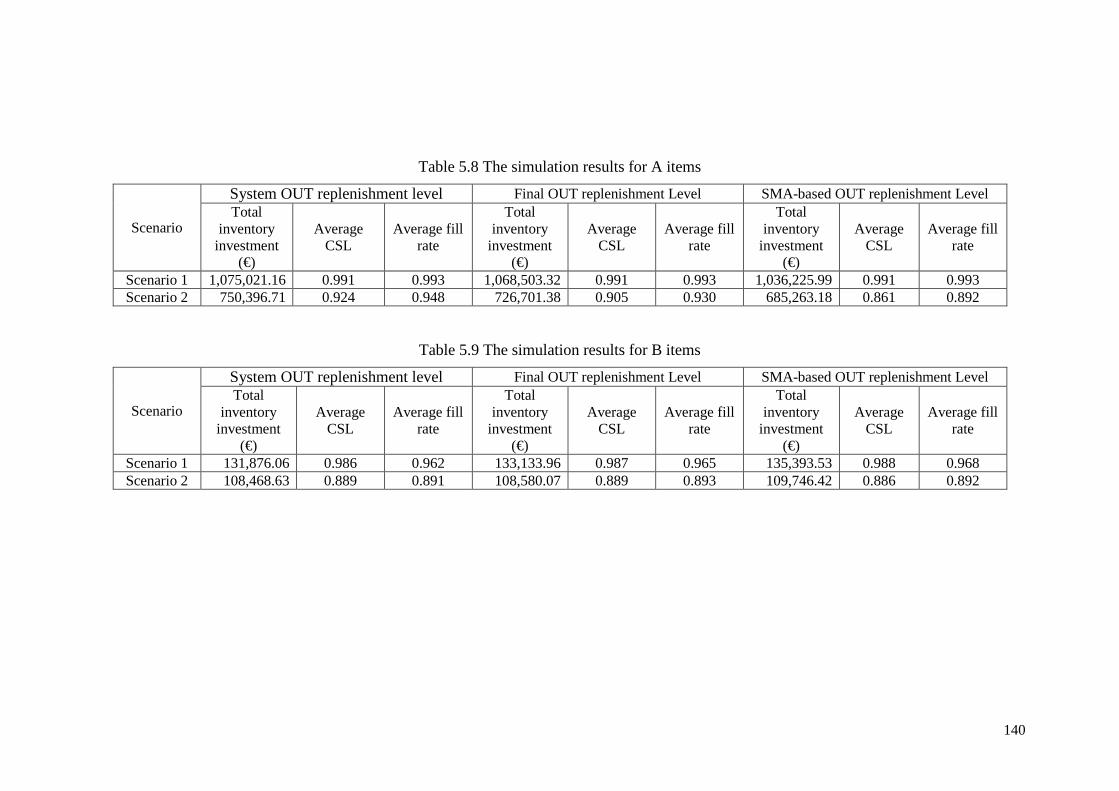
140
Table 5.8 The simulation results for A items
Scenario
System OUT replenishment level Final OUT replenishment Level SMA-based OUT replenishment Level Total
inventory investment
(€)
Average CSL
Average fill rate
Total inventory
investment (€)
Average CSL
Average fill rate
Total inventory
investment (€)
Average CSL
Average fill rate
Scenario 1 1,075,021.16 0.991 0.993 1,068,503.32 0.991 0.993 1,036,225.99 0.991 0.993 Scenario 2 750,396.71 0.924 0.948 726,701.38 0.905 0.930 685,263.18 0.861 0.892
Table 5.9 The simulation results for B items
Scenario
System OUT replenishment level Final OUT replenishment Level SMA-based OUT replenishment Level Total
inventory investment
(€)
Average CSL
Average fill rate
Total inventory
investment (€)
Average CSL
Average fill rate
Total inventory
investment (€)
Average CSL
Average fill rate
Scenario 1 131,876.06 0.986 0.962 133,133.96 0.987 0.965 135,393.53 0.988 0.968 Scenario 2 108,468.63 0.889 0.891 108,580.07 0.889 0.893 109,746.42 0.886 0.892
141
Comparing the inventory investment of SMA-based OUT replenishment level with the
adjusted one, it can be seen that the latter produces lower cost, but the difference is indeed
very small: 1.67% (€2,260) in scenario 1 and 1.06% (€1,166) in scenario 2. However, and
although this naturally leads to a slight decrease in the service measures under scenario 1,
in scenario 2 the opposite occurs. This, in theory, indicates that adjustments lead not only
to less safety stocks (as expressed through the inventory investment) but also to better
service provision. It is true that the differences observed are very small but nevertheless the
results favour conclusively the judgementally adjusted OUT levels.
The above findings are consistent with the results presented in most relevant studies in the
forecasting field where judgemental adjustments seems to account for (considerable)
performance improvement (Diamantopoulos and Mathews, 1989; Mathews and
Diamantopoulos, 1986, 1990, 1992; Lawrence et al., 1986; Angus-Leppan and Fatseas,
1986; Wolfe an Flores, 1990; Syntetos et al., 2009b). However, the results indicate that
there may be less benefit resulting from judgementally adjusting stock control decisions
than statistical demand forecasts. This finding is in agreement with the Syntetos et al.
(2011) findings which showed that judgemental forecast adjustments have more prominent
effects than judgemental order adjustments.
From the above discussion we may provide an answer to the first research question, about
the potential performance improvement resulting from judgementally adjusting stock
control-related decisions; we find that human intervention seems to offer a reasonable
advantage in stock control decision making.
5.6. The effects of the sign of adjustments on inventory performance
The purpose of this analysis is to evaluate the effects of the sign of adjustments
(positive/increasing adjustment and negative/decreasing adjustment) on inventory
142
performance. To conduct such analysis, we consider the average adjustment per SKU
across time as it would simply be impractical to analyse the effects of each adjustment
separately. The average adjustment is used to classify SKU into two categories: positive
and negative average adjustment. The next step is to analyse the inventory performance for
each of these two groups in terms of inventory investment, cycle service level (CSL) and
fill rate across all the SKUs in that group. The results are shown in Table 5.10 and Table
5.11 for the A and B items respectively.
The results of simulation for the A items indicate that the inventory investment related to
the adjusted replenishment orders is lower than that corresponding to the System OUT
replenishment orders with the exception of the positive adjustment category in scenario 1.
Regarding the service measures, there is no significant difference between the two
replenishment order methods for scenario 1. Whereas for scenario 2, the service level and
fill rate of adjusted replenishment orders tends to be lower than the unadjusted ones,
particularly for the positive adjustment category. Thus, we may say that the negative
adjustments perform better than the positive ones in improving the performance of the
inventory system. In addition, we may see that there is always a trade-off between cost and
service level.

143
Table 5.10 The effect of sign adjustments on inventory performance for A items
Scenario Classification
System OUT replenishment level Final OUT replenishment Level SMA-based OUT replenishment Level
Total inventory investment
(€)
Average CSL
Average fill rate
Total inventory
investment (€)
Average CSL
Average fill rate
Total inventory
investment (€)
Average CSL
Average fill rate
Scenario 1 Negative 68,967.05 0.997 0.997 67,733.45 0.997 0.997 66,237.29 0.997 0.997 Positive 7,774.83 0.977 0.983 7,932.64 0.979 0.984 7,996.25 0.978 0.984
Scenario 2 Negative 63,344.46 0.944 0.965 62,258.97 0.932 0.952 61,340.38 0.887 0.910 Positive 4,687.58 0.877 0.908 4,493.26 0.842 0.878 4,476.91 0.800 0.851
Table 5.11 The results of sign adjustments on inventory performance for B items
Scenario Classification
System OUT replenishment level Final OUT replenishment Level SMA-based OUT replenishment Level
Total inventory
investment (€)
Average CSL
Averagefill rate
Total inventory
investment (€)
Average CSL
Averagefill rate
Total inventory
investment (€)
Average CSL
Averagefill rate
Scenario 1 Negative 56,492.58 0.990 0.968 56,466.85 0.990 0.969 54,478.44 0.991 0.971 Positive 10,308.45 0.975 0.947 10,551.40 0.978 0.956 10,644.65 0.979 0.958
Scenario 2 Negative 50,222.58 0.907 0.916 50,084.03 0.904 0.913 49,564.00 0.904 0.910 Positive 8,159.44 0.835 0.818 8,322.16 0.843 0.833 8,426.52 0.832 0.840
144
For B items, the negative adjustment category for Final OUT replenishment level produced
lower inventory investment compare to System OUT level. For scenario 1, this category is
not associated with much difference of CSL and fill rate between the Final OUT
replenishment level and System OUT replenishment level. Whereas in scenario 2, we find
that the Final OUT replenishment level has lower values of CSL and fill rate. On the other
hand, the inventory investment on the positive adjustment category of the adjusted
replenishment orders is higher than the unadjusted ones. The increase on both scenarios is
between €162.72 and €242.95. It raises the CSL by 0.31% to 0.95%, and fill rate by 0.94%
and 1.80%. Thus, as the results are the same with the A-class items we may conclude that
negative adjustments may deliver more benefit than the positive adjustments towards the
improvement of inventory system.
The comparison between the SMA-based OUT replenishment level and the Final OUT
replenishment level indicates that the negative adjustments seem to increase the inventory
investment whereas the opposite is true for positive adjustments.
Regarding CSL and fill rate, the experiment results produce similar values, except for the
value of scenario 2 of A items where the CSL and fill rate of SMA-based OUT
replenishment level is significantly lower than the Final OUT replenishment level.
Moreover, the Final OUT replenishment level seems to be associated with better CSL and
fill rate than the SMA-based OUT replenishment level on both signs of adjustment, except
from scenario 1. It can be seen that for A items in scenario 1, and for B items in both
scenarios, the CSL and fill rate increases between 0.0 - 0.045, while the decrease is only
between -0.001 to -0.002 for A items in scenario 2. This indicates that, even when SKUs
are categorised by the sign of adjustments, the adjusted replenishment orders perform
better than the SMA-based OUT replenishment level ones.

145
The results also show that the values of CSL and fill rate with negative adjustments seem
higher than those with positive adjustments for each scenario for both categories of items.
This result is in line with the findings of judgemental forecasting research which has found
that large negative adjustments perform well in increasing forecast accuracy for products
that are subject to intermittent demand (Syntetos et al., 2009b) and also for fast moving
demand (Fildes et al., 2009). These forecasting studies argued that negative adjustments
are more effective than positive adjustments since they reflect genuinely important pieces
of information. Furthermore, the relatively poor performance of positive adjustments may
be a result of an optimism bias on the part of the forecasters (the issue of bias in
judgementally adjusted replenishment order decisions will be discussed in section 5.9).
Forecasters tend to over-weight the statistical system’s forecast when contextual
information is available (but in the absence of reliable evidence). Alternatively, excessive
upward adjustments may be motivated by political factors such as pressure from senior
management. Insights from the judgemental forecasting research cited above may explain
why negative adjustments on replenishment order decisions perform better than positive
adjustments.
In the case of this company, managers tend to decrease the OUT level of A items mostly
between [0- −20] units (see analysis in section 5.3 above). For B items, however, most
adjustments made by the manager are between [0-10] units. This indicates that negative
adjustments occur more on A items than B items. This result is consistent with the value of
CSL and fill rate resulting from the Final OUT replenishment level for each category. If we
compare the average CSL and fill rate of the Final OUT replenishment level between A
items and B items, we find that A items have greater values than B items (CSL for A and B
items is 0.938 and 0.929 respectively; fill rate for A and B items is 0.953 and 0.918
respectively).

146
5.7. The effects of the absolute size of adjustments on inventory performance
Two pieces of analysis are conducted to explore the effects of the size of adjustments. The
first one is conducted using the average of the absolute size of the adjustments (the sign of
adjustments is not considered in calculating the average). The second relates to the
absolute average size of the adjustments (taking the average size of the adjustments,
considering the positive/negative sign of adjustments, and then calculating the absolute
value of that average). After calculating the average of absolute and average of absolute
signed adjustments, the next step is to calculate the percentage adjustment from the
average demand for every SKU for the purpose of classifying the SKUs into small,
medium, and large adjustments categories. For this categorisation, we consider these to be:
i) small adjustments if: 0 < average adjustment/average demand ≤ 10%,
ii) medium adjustments if: 10% < average adjustment/average demand ≤ 20%,
iii) large adjustments if: average adjustment/average demand > 20%.
Then the inventory performance (inventory investment, CSL, and fill rate) is compared for
each category in every scenario. This performance analysis is based on the average of the
adjustment across time since the signs of adjustments for each SKU cannot be useful.
5.7.1. The average of the absolute size of the adjustments
After obtaining the results of average adjustment/average demand for each SKU, we find
that the above grouping does not fit the range of average absolute adjustment of B items.
The smallest value of average adjustment/average demand is 11.18%. As a result, for B
items, we change the grouping into: less than or equal to 20% for small adjustments,
between 20% and 40% for medium adjustments, and above 40% for large adjustments.
Applying this new grouping to A items is not inappropriate because the highest
adjustment/average demand value is 38.07%. Thus, the categorisation for A items stays as
discussed above in 5.7.
147
Table 5.12 and Table 5.13 show the inventory performance analysis results for A and B
items respectively.
The simulation results indicate that, for A-class items, the inventory investment of adjusted
replenishment orders is lower than that associated with unadjusted replenishment orders. In
term of CSL and fill rate, the Final OUT replenishment levels are associated with the same
or higher values than the System OUT replenishment level related ones, for scenario 1.
This indicates that the adjusted replenishment orders decrease the inventory cost whilst
resulting in higher customer service level and fill rate. However, this is not the case for
scenario 2. The decrease of inventory cost also results to the decrease of CSL and fill rate
value.
Further analysis on the size of the adjustment for both scenarios reveals that ‘large
adjustment’ category (higher than 20%) results to the best performance as the decrease of
inventory cost is not accompanied by an expected decrease of service provision.

148
Table 5.12 The results of absolute of adjustment on the inventory performance analysis for A items
Scenario Classification
System OUT replenishment level Final OUT replenishment Level SMA-based OUT replenishment Level
Total inventory
investment (€)
Average CSL
Average fill rate
Total inventory investment
(€)
Average CSL
Average fill rate
Total inventory
investment (€)
Average CSL
Average fill rate
Scenario 1
< 10% 24,067.72 0.991 0.993 23,847.71 0.991 0.993 23,250.42 0.992 0.993 10-20% 21,455.81 0.985 0.989 21,206.15 0.989 0.991 20,268.10 0.986 0.991 >20% 32,000.71 1.000 1.000 31,304.22 1.000 1.000 31,300.42 1.000 1.000
Scenario 2
< 10% 17,691.09 0.921 0.950 17,087.29 0.898 0.928 16,053.79 0.862 0.893 10-20% 18,962.38 0.910 0.922 18,420.20 0.903 0.916 18,455.09 0.810 0.853 >20% 31,378.56 1.000 1.000 31,244.74 1.000 1.000 31,308.42 1.000 1.000
Table 5.13 The results of absolute of adjustment on the inventory performance analysis for B items
Scenario Classification
System OUT replenishment level Final OUT replenishment Level SMA-based OUT replenishment Level
Total inventory
investment (€)
Average CSL
Average fill rate
Total inventory
investment (€)
Average CSL
Average fill rate
Total inventory
investment (€)
Average CSL
Average fill rate
Scenario 1
< 20% 646.82 1.000 1.000 655.42 1.000 1.000 791.41 1.000 1.000 20-40% 4,936.22 0.988 0.987 4,964.34 0.988 0.988 5,281.42 0.990 0.989 >40% 61,276.45 0.985 0.949 61,456.04 0.986 0.953 59,107.47 0.987 0.956
Scenario 2
< 20% 557.58 0.983 0.997 560.30 0.988 0.998 664.07 0.983 0.995 20-40% 4,215.67 0.897 0.915 4,221.67 0.897 0.919 4,314.99 0.906 0.927 >40% 53,658.98 0.879 0.873 53,672.81 0.879 0.874 53,068.26 0.870 0.870

149
The opposite result was found for B-class items where adjusted replenishment orders seem
to be associated with a higher inventory investment compared to the unadjusted ones
although the differences are very small (mostly less than 0.5%). The slight increase in cost
also results in a small improvement of the CSL and fill rate. From the results we may see
that the best performance is resulting from the ‘large adjustment’ category; the smallest
increase in inventory investment may result in the highest CSL and fill rate as compared to
other categories.
From the comparative analysis of SMA-based OUT replenishment levels and Final OUT
replenishment level, we found that for A items, the inventory investment of SMA-based
OUT replenishment levels is lower than the Final OUT replenishment levels for all of the
adjustments categories when considering scenario 1.In scenario 2, this is true only for the
‘small adjustment’ category. Different results were found for B items, where the inventory
investment of SMA-based OUT replenishment level is usually higher than the Final OUT
replenishment level related one in the small and medium adjustment categories.
In term of service level and fill rate of A items, the same values are found between the
SMA-based OUT replenishment level and Final OUT replenishment level for scenario 1.
However, most of CSL and fill rate associated with the Final OUT replenishment levels
seem to be higher compare with the SMA-based ones in scenario 2. Moreover, the highest
service level and fill rate is resulted from the ‘medium adjustment’ category. However, it is
difficult to make a conclusion regarding the CSL and fill rate for B items since no pattern
can be found in the simulation results.
5.7.2. The absolute average size of the adjustments
Table 5.14 shows the result of the analysis on the absolute average size of adjustments of
A items. It can be seen that generally Final OUT replenishment levels result in lower
inventory investment compared to System OUT replenishment levels. The decrease is
150
between 0.23% and 6.88%. The decrease of inventory investment produces only a slight
increase of CSL and fill rate for scenario 1. The lowest inventory investment is resulted
from the large (>20%) adjustment category. However, in scenario 2 the decrease of
inventory investment also produces lower CSL and fill rate.
In Table 5.15 we can see the simulation result for B items. Most of the inventory
investments of Final OUT replenishment levels are higher than the System OUT
replenishment level ones, which consequently increase the CSL and fill rate except for the
large adjustment category in scenario 2.
Moreover, it can be seen that the inventory investment of SMA-based OUT replenishment
levels is generally lower than that associated with the Final OUT replenishment levels in
the medium and large adjustment categories. On the other hand, inventory investment of
SMA-based OUT replenishment levels seems to have higher values than the Final OUT
replenishment levels one for the SKU in the ‘small adjustments’ category. In addition, the
highest service level and fill rate results from the ‘large adjustments’ category for A items
and medium and large categories for B items.

151
Table 5.14 The results of absolute signed of adjustments on the inventory performance analysis for A items
Scenario Classification
System OUT replenishment level Final OUT replenishment Level SMA-based OUT replenishment Level
Total inventory
investment (€)
Average CSL
Average fill rate
Total inventory
investment (€)
Average CSL
Average fill rate
Total inventory
investment (€)
Average CSL
Average fill rate
Scenario 1 < 10% 7,404.17 0.991 0.992 7,387.28 0.991 0.992 7,436.89 0.991 0.992 10-20% 6,281.54 0.985 0.990 6,333.51 0.986 0.993 6,213.64 0.986 0.992 >20% 63,838.53 0.993 0.994 62,637.28 0.994 0.994 61,168.40 0.994 0.994
Scenario 2 < 10% 4,279.89 0.934 0.944 3,985.36 0.900 0.915 4,052.60 0.833 0.858 10-20% 3,061.30 0.890 0.944 2,972.39 0.863 0.935 2,647.93 0.848 0.898 >20% 58,982.36 0.932 0.953 58,093.04 0.928 0.946 57,430.49 0.888 0.915
Table 5.15 The effects of absolute signed of adjustments for B items
Scenario Classification
System OUT replenishment level Final OUT replenishment Level SMA-based OUT replenishment Level
Total inventory
investment (€)
Average CSL
Average fill rate
Total inventory
investment (€)
Average CSL
Average fill rate
Total inventory
investment (€)
Average CSL
Average fill rate
Scenario 1 < 10% 7,947.48 0.983 0.970 7,960.87 0.985 0.976 7,930.56 0.987 0.979 10-20% 4,243.13 0.982 0.971 4,428.07 0.983 0.977 4,575.42 0.987 0.984 >20% 54,610.42 0.990 0.955 54,629.30 0.990 0.955 52,617.11 0.989 0.955
Scenario 2 < 10% 5,933.73 0.877 0.876 5,995.12 0.880 0.883 6,181.46 0.875 0.874 10-20% 3,716.33 0.916 0.915 3,795.88 0.921 0.924 3,774.87 0.914 0.930 >20% 48,731.96 0.886 0.891 48,615.19 0.883 0.888 48,034.19 0.882 0.890

152
The results on inventory investment for A and B items suggest that the extent of the
advantage associated with the size of adjustments is not yet clear, because the results of the
analysis for both classes of items, both scenarios, and both types of descriptive
summarization considered (absolute and absolute sign) are too varied. However, if we
focus on the CSL and fill rate, we may say that for A items, the performance of the ‘large
adjustments’ group is higher than that of other groups, whereas medium and large
adjustment categories perform better on B items.
In the area of judgemental forecasting, Fildes et al. (2009) argued that large adjustments
may improve forecast accuracy more effectively than small adjustments since the small
adjustments are merely a response to non-existing patterns. The same results are also found
by Diamantopoulos (1986, 1990, 1992), and Diamantopoulos and Mathews (1989).
Moreover, O’Connor and Lawrence (1989) found that judgemental confidence intervals in
time series forecasting were initially excessively over-confident. This situation may also
exist in judgemental stock control decision making where the large adjustments might only
represent overreaction by the decision maker in response to the available contextual
information.
For B items, as we mentioned above, large and medium adjustments perform better for
CSL and fill rate values but not for reducing inventory investment. If the organisation
focuses on the achievement of service level target, thus the manager needs to be very
careful with the small adjustments since the wrong decision made by the manager on B
items will directly increase the holding cost (due to the analysis result of price of materials
explained in section 5.2 that shows the most B items are more expensive than A items).
In the forecasting field, the decision maker needs to consider adjustments based on
statistical forecasting and also estimates of the size of the adjustment (Lawrence et al.,
2006).From these findings we may say that the benefits of making adjustments on stock

153
control decisions not only depends on the size of adjustments made by the manager, but
also on the demand characteristics of the item.
In addition, the procedure for calculating the absolute size of adjustments is also the factor
that affects the results of this analysis. For example, the above analyses (absolute
adjustments and absolute sign adjustments) offers significantly (not in a statistical sense)
different experiment results of A and B items for both scenarios. These differences
introduce complications towards the interpretation of the results and reaching specific
conclusions. In the forecasting area, conflicting results due to different forecasting
accuracy measurements (percentage errors, relative errors, and scaled errors) often occur
since each measure is associated with specific limitations. The inconsistency of the results
may also be due to the nature of the demand data. This issue is investigated by Davydenko
and Fildes (2013) that suggest that the well-known forecast error measures seem not
suitable for judgemental adjustment forecasting and then attempt to develop an appropriate
procedure for measuring judgemental forecasting accuracy.
5.8. The effects of justification of adjustments on inventory performance
This part of the analysis examines the effects of the reasons for adjustments on inventory
performance. It is achieved by calculating the number of justification adjustments for each
SKU. Then, the adjustments are separated into four categories based on the number of
justifications for the adjustments:
i) Justifications <25%;
ii) 25%<Justifications<50%;
iii) 50%<Justifications<75%;
iv) Justifications>75%.

154
Furthermore, the inventory performance (inventory investment, CSL and fill rate) is
compared for each category in every scenario.
Table 5.16 and Table 5.17 show the results associated with the justification for the
adjustments on the inventory performance for A and B-class items respectively.
By comparing the inventory investment associated with the System OUT replenishment
levels and the Final OUT replenishment levels of A-class, we found that, in the majority of
cases all justification categories result in lower inventory investments without that
implying a decrease in the service provision. In fact the opposite is the case.
For B-class items, regarding the inventory investment, SKUs which are associated with
justifications between 25% and 50% for scenario 1 and those between 25% and 75% for
scenario 2 seems to be associated with the best comparative performance. The decrease in
inventory investment in the particular categories resulted to a positive contribution to CSL
and fill rate.
In terms of CSL and fill rate, it can be seen from scenario 1 in Table 5.16 that the same
CSL and fill rate values are obtained for both replenishment order procedures. Moreover,
in scenario 2, for A-class items, the CSL and fill rate associated with the Final OUT
replenishment levels tend to be higher than that related to the SMA-based OUT
replenishment levels. A considerable increase of the CSL and fill rate values from the
SMA-based OUT replenishment levels to adjusted replenishment orders were found on the
SKUs that have justification more than 75%. The increase of CSL and fill rate under this
category is 16.7% and 18.9% respectively. For B items, the results are varied. However,
we can see that the highest increase in CSL and fill rate when moving from the SMA-based
OUT replenishment levels to Final OUT replenishment levels is given by SKUs that have
justification more than 75%, which is the same as the result for A items.

155
Table 5.16 The results of justification of adjustments on the inventory performance analysis for A items
Scenario Classification
System OUT replenishment level Final OUT replenishment Level SMA-based OUT replenishment Level
Total inventory
investment (€)
Average CSL
Average fill rate
Total inventory
investment (€)
Average CSL
Average fill rate
Total inventory
investment (€)
Average CSL
Average fill rate
Scenario 1
Just <25% 1,455.67 1.000 1.000 1,437.63 1.000 1.000 1,448.40 1.000 1.000 25%<Just<50% 45,301.16 0.992 0.994 44,227.83 0.992 0.994 42,661.12 0.992 0.994 50%<Just<75% 30,439.24 0.979 0.980 30,374.31 0.980 0.981 30,348.16 0.980 0.981
Just>75% 328.18 1.000 1.000 318.30 1.000 1.000 361.24 1.000 1.000
Scenario 2
Just <25% 2,302.08 0.991 0.997 6,645.19 0.943 0.938 6,536.40 0.944 0.943 25%<Just<50% 51,912.72 0.921 0.947 52,030.02 0.900 0.925 49,443.21 0.850 0.881 50%<Just<75% 18,831.17 0.883 0.914 13,913.56 0.891 0.939 13,054.94 0.841 0.899
Just>75% 143.01 1.000 1.000 127.87 1.000 1.000 63.39 0.833 0.811
Table 5.17 The results of justification of adjustments on the inventory performance analysis for B items
Scenario Classification
System OUT replenishment level Final OUT replenishment Level SMA-based OUT replenishment Level
Total inventory
investment (€)
Average CSL
Average fill rate
Total inventory
investment (€)
Average CSL
Average fill rate
Total inventory
investment (€)
Average CSL
Average fill rate
Scenario 1
Just <25% 31,416.74 0.986 0.958 31,681.23 0.986 0.960 30,440.71 0.988 0.964 25%<Just<50% 15,963.83 0.988 0.970 15,882.38 0.990 0.973 15,622.48 0.990 0.974 50%<Just<75% 18,831.69 0.982 0.962 18,856.64 0.987 0.970 18,545.67 0.985 0.967
Just>75% 588.76 0.992 1.000 598.00 0.992 1.000 514.23 0.992 1.000
Scenario 2
Just <25% 25,935.91 0.887 0.887 25,969.53 0.886 0.885 25,545.11 0.879 0.881 25%<Just<50% 14,814.54 0.914 0.907 14,810.91 0.916 0.915 14,775.70 0.917 0.919 50%<Just<75% 17,507.99 0.875 0.881 17,498.92 0.875 0.888 17,532.18 0.893 0.897
Just>75% 123.58 0.650 0.827 126.83 0.667 0.850 137.52 0.642 0.847

156
The above findings show that the SKUs associated with more than 75% justifications
produce the highest stock control performance. The reasons or justifications behind
managers changing the OUT level produced by the software system in the past may be the
factor that helps the decision maker to make adjustments. In their forecasting study, Onkal
et al. (2008) reported that the explanation accompanying the adjusted forecasts helps the
decision maker to define the appropriate size of adjustments and gives more benefits from
further modifications. Moreover, this may be useful in the learning process for
practitioners towards an understanding of why decisions may be erroneous (Stekler, 2007).
Levitt and March (1996) argued that the procedure to store and access information,
particularly when forecasters seek to make judgements, is the important consideration in
the documentation of contextual information. The case organisation has documented some
of the justifications for the adjustments made by managers; however, managers seem to
change the OUT level frequently without giving any reason (see the justification of
adjustment analysis in section 5.4). As we know that the case organisation does not
document the reason for adjustment in detail, and is indeed unaware of the importance of
contextual information (for convenience they always report the same justification), it is
recommended that the company improves its documentation procedure in order improve
their judgemental stock control performance. The justification for adjustments should be
determined not only when the decision maker makes an adjustment, but also how,
presenting the reason why judgement is incorporated into the decision. These factors are
important to reduce bias in judgemental adjustment forecasting (Goodwin, 2000), and may
also be important in judgemental stock control systems. The above discussion may answer
our research question about improving stock control performance by the adjustments when
justification is offered on adjusted replenishment order decisions, since we found that the
SKUs associated with more justifications are also associated with better performance.

157
5.9. The effect of bias of adjustments on inventory performance
Many studies have investigated bias in judgementally adjusting forecasts (for example
Diamantopoulos and Mathews, 1990; Mathews and Diamantopoulos, 1990; Goodwin and
Wright, 1994) although based on our knowledge so far, there is no study about this issue in
the stock control area. Thus, in making judgemental adjustments, managers tend to use
heuristic principles while taking contextual information into consideration. Heuristic
principles have systematic errors (Tversky and Kahneman, 1974).
For this analysis, identification of bias of adjustments on inventory performance is
achieved by calculating the average adjustments per SKU (across time). Then the
maximum and minimum values of adjustments are defined. The next step is to calculate
the value of 10% of the maximum of negative adjustments and 10% of the minimum of
positive adjustments, to classify the average of adjustment as positive biased, unbiased or
negative biased. For this categorisation, we consider:
- Positive biased if the average adjustment per SKU > 10% max
- Unbiased if min 10% < the average adjustment per SKU < 10% max
- Negative biased if the average of adjustment per SKU < 10% min
Next, the average of inventory performance between groups is compared.
Table 5.18 and Table 5.19 show the results of bias on the inventory performance analysis
for A and B-class items respectively.
For A items, it can be seen that inventory investments associated with the Final OUT
replenishment level are generally lower than that the System OUT replenishment level
ones for both scenarios. With regards to the CSL and fill rate, in scenario 1, we found that
there are no differences between the Final OUT replenishment levels and the System OUT
replenishment levels with the exception of the ‘positive biased adjustment’ category.
Whereas for scenario 2 we found that the service level and fill rate of the Final OUT

158
replenishment levels seems to have a lower value than that of the System OUT
replenishment level for all adjustment categories. Moreover, we can conclude from this
analysis that the ‘negative biased adjustment’ category perform well in improving the
performance of the inventory system since this category resulted in the lowest inventory
investment and does not imply (or it does only marginally) a reduction of the CSL and fill
rate.
In the analysis of B items we found that the inventory investment of the Final OUT
replenishment levels seems to be lower than that of the System OUT replenishment levels
only in the ‘negative biased adjustment’ category for both scenarios. In this category, for
scenario 1, the CSL and fill rate value is the same for both replenishment order methods.
For scenario 2, the ‘negative biased adjustment’ category did not affect much the CSL and
fill rate value. This indicates that negative bias results in better results than the other
categories. It means that, if the managers make adjustments without any rationale or adjust
the OUT level in arbitrary way, the negative adjustments seems perform better compare to
the positive ones. This finding is in line with the sign of the adjustments analysis in section
5.6 where we found that the negative adjustments produce the best performance.
When comparing the SMA-based OUT replenishment levels and the Final OUT
replenishment levels, we can see that the inventory investment of the former is lower than
that of the latter for the negative biased and unbiased adjustments categories, whereas for
the positive biased category, the opposite is the case Furthermore, in terms of the CSL and
fill rate, it can be seen from Table 5.18 that the highest CSL and fill rate for A items
resulted from the negative bias adjustments category for both scenarios. For B items, the
highest CSL and fill rates were produced by the unbiased adjustments category. For all
items, it also appears that the ‘positive-biased adjustments’ category produced the lowest
CSL and fill rate. This finding seems to be consistent with research on judgemental
159
forecasting by Syntetos et al. (2009b) who found that positive adjustments lead to
unsatisfactory performance of the inventory system; they argued that optimistic bias would
lead to positive adjustments being made in the absence of reliable evidence that the
forecast does need an upward adjustment, or lead to over-enthusiastic upward adjustment
when such evidence was available. Moreover, there is evidence in judgemental adjustment
forecasting that the source of contextual information constitutes a major factor that
influences the frequency and magnitude of adjustments (Onkal, et al., 2013). In that study,
the source of information based on direct experience gives more effects on the level of
adjustment compared with the information based on assumption. This phenomenon might
also take place when judgementally adjusting stock replenishment decisions.
The above discussion implies that biases also exist in the area of judgementally adjusting
replenishment decisions. This may answer our fourth research question, i.e. whether or not
judgementally adjusted stock control decisions are associated with bias. In addition, in
order to obtain the benefits of making adjustments in stock control decisions, it is
important to understand the nature of decision biases in deciding how to manage those
biases in the process (Carter et al., 2007).

160
Table 5.18 The results of the bias of adjustments on the inventory performance analysis for A items
Scenario Classification
System OUT replenishment level Final OUT replenishment Level SMA-based OUT replenishment Level
Total inventory
investment (€)
Average CSL
Average fill rate
Total inventory
investment (€)
Average CSL
Average fill rate
Total inventory
investment (€)
Average CSL
Average fill rate
Scenario 1
Negative biased 200.66 1.000 1.000 196.54 1.000 1.000 180.84 1.000 1.000 Unbiased 76,697.36 0.992 0.993 75,559.27 0.992 0.993 74,080.02 0.992 0.993 Positive biased 297.76 0.968 0.985 330.02 0.972 0.987 360.68 0.968 0.989
Scenario 2
Negative biased 346.06 0.995 0.999 311.92 0.990 0.996 271.45 0.943 0.967 Unbiased 67,585.39 0.929 0.948 66,348.49 0.910 0.930 65,453.68 0.861 0.888 Positive biased 100.58 0.769 0.909 91.81 0.727 0.866 92.15 0.782 0.897
Table 5.19 The results of the biased on adjustments on the inventory performance analysis for B items
Scenario Classification
System OUT replenishment level Final OUT replenishment Level SMA-based OUT replenishment Level
Total inventory
investment (€)
Average CSL
Average fill rate
Total inventory
investment (€)
Average CSL
Average fill rate
Total inventory
investment (€)
Average CSL
Average fill rate
Scenario 1
Negative biased 475.18 0.990 0.946 461.94 0.990 0.946 437.83 0.990 0.946 Unbiased 64,983.96 0.989 0.969 65,128.63 0.990 0.972 63,135.88 0.990 0.974 Positive biased 1,341.89 0.968 0.927 1,427.67 0.968 0.933 1,549.38 0.973 0.942
Scenario 2
Negative biased 392.58 0.869 0.885 383.19 0.867 0.881 371.04 0.888 0.901 Unbiased 57,021.83 0.904 0.911 57,029.50 0.902 0.910 56,619.65 0.900 0.904 Positive biased 967.61 0.796 0.755 993.50 0.813 0.782 999.82 0.785 0.801

161
5.10. Learning effects of making adjustments on inventory performance
The analysis of learning effects is conducted in order to evaluate whether there are such
effects in the process of superimposing judgement into inventory related decisions. The
analysis is based on the number of adjustments to each SKU (assuming that there is only
one person dealing with each SKU) followed by their grouping in three categories as
follows:
i) Low: number of adjustments ≤13
ii) Medium: 13 < number of adjustments ≤ 21
iii) High: number of adjustments >21.
We then compare the inventory performance resulting in these three groups, assuming the
more adjustments are associated with a higher learning effect (the more the process of
adjusting is repeated, the more the individual who performs the adjustments learns and the
better s/he performs.)
From Table 5.20 we can see that, for A-class items, judgemental adjustments generally
lead to inventory investment reductions. The lowest inventory investment value resulted
from the ‘medium adjustments’ category for both scenarios. In terms of CSL and fill rate,
we may say that, for scenario 1, there is no difference between unadjusted and adjusted
replenishment orders. For scenario 2, the CSL and fill rate of System OUT replenishment
levels seems to have higher values as compared to the Final OUT replenishment levels for
medium and high number of adjustments category. Since a high number of adjustments do
not improve the inventory system performance, we may conclude that there is no learning
effect taking place in A-class items.
Table 5.21 shows the simulation results for the B-class items. It can be seen that the
inventory investment associated with the Final OUT replenishment levels is higher than

162
that related to System OUT replenishment levels. For scenario 1, the CSL and fill rate of
the former is also higher than that of the latter, whereas the opposite is the case for scenario
2. The medium and high numbers of adjustment categories seem to perform better than the
small number of adjustment category. Thus, we may conclude that for B items there is an
occurrence of learning effect.
In the comparison between the Final OUT replenishment levels and the SMA-based OUT
replenishment levels for the A items, the inventory investment of the latter is lower than
that of the former (except for the ‘low adjustments category’ in scenario 1). However, for
B items, the same is the case for the low and medium adjustments categories in scenario 1,
and also for the ‘low adjustment category’ in scenario 2.
Regarding the CSL and fill rate values, it can be seen that the highest value of CSL and fill
rate for A items is found in the ‘low adjustment category’, whereas for B items this mostly
occurs in the ‘high adjustment category’. As a result, we may say that there is no learning
effect associated with A items since the high number of adjustments does not lead to a
better performance. For instance, when considering the Final OUT replenishment level of
scenario 1, as the number of adjustments increases, the CSL and fill rate decrease.
On the other hand, it does appear to be a learning effect when the manager makes
adjustments on replenishment order decisions for B items, as shown by the increase in the
value of SCL and fill rate as the number of adjustments becomes higher. From Table 5.21
we can see that the highest CSL and fill rate for both scenarios mostly results from the
‘high number of adjustments’ category. For example, in scenario 2 the fill rate increases
from 0.830 in the low adjustments category to 0.931 in the high adjustments category.

163
Table 5.20 The results of learning-effects analysis based on number of adjustments for A items
Scenario Classification
System OUT replenishment level
Final OUT replenishment Level SMA-based OUT replenishment Level
Total inventory
investment (€)
Average CSL
Average fill rate
Total inventory
investment (€)
Average CSL
Average fill rate
Total inventory
investment (€)
Average CSL
Average fill rate
Scenario 1
adjustment <=13 7,725.17 1.000 1.000 7,645.70 1.000 1.000 7,694.58 1.000 1.000 <13adjustment <=21 67,902.07 0.993 0.992 66,749.48 0.993 0.992 65,205.44 0.993 0.992
adjustment >21 1,897.00 0.981 0.992 1,962.90 0.982 0.993 1,918.91 0.982 0.994
Scenario 2
adjustment <=13 7,637.98 1.000 1.000 7,618.45 1.000 1.000 7,578.94 1.000 1.000 <13adjustment <=21 59,134.21 0.933 0.947 57,890.62 0.913 0.928 57,080.39 0.863 0.887
adjustment >21 1,259.84 0.870 0.942 1,243.15 0.852 0.924 1,157.95 0.828 0.894
Table 5.21 The results of learning-effects analysis based on number of adjustments for B items
Scenario Classification
System OUT replenishment level
Final OUT replenishment Level SMA-based OUT replenishment Level
Total inventory
investment (€)
Average CSL
Average fill rate
Total inventory
investment (€)
Average CSL
Average fill rate
Total inventory
investment (€)
Average CSL
Average fill rate
Scenario 1
adjustment <=13 30,817.08 0.986 0.869 30,893.03 0.986 0.869 30,459.94 0.986 0.872 <13adjustment <=21 32,837.03 0.987 0.967 32,917.83 0.988 0.970 31,298.49 0.988 0.971
adjustment >21 3,205.38 0.986 0.980 3,264.94 0.987 0.984 3,421.88 0.988 0.988
Scenario 2
adjustment <=13 29,305.22 0.885 0.834 29,339.33 0.878 0.830 28,871.79 0.854 0.834 <13adjustment <=21 26,495.99 0.870 0.876 26,444.98 0.867 0.873 26,504.54 0.867 0.871
adjustment >21 2,631.02 0.910 0.922 2,670.48 0.916 0.931 2,670.99 0.915 0.930

164
The above findings indicate that demand characteristics may affect the presence of learning
effects. The judgemental adjustments for A items, which are less intermittent than B items,
do not improve over time. This result is consistent with the findings of studies of
judgmentally adjusted forecasts where no learning effect is found in the forecasting
function (Syntetos et al, 2009b). Moreover, Nikolopoulos et al. (2006) show that there are
gaps in the learning loop in the forecasting systems (adjusted and unadjusted) since
forecasters in companies are not trained sufficiently over time (Lim and O’Connor, 1996;
Klassen and Flores, 2001).
The performance of the inventory system for A items does not improve over time most
probably because of the inability of the managers to use contextual information and/or
experience when making adjustments. In judgemental forecasting research, Nikolopoulos
et al. (2006) state that forecasting error cannot be eliminated, because of specific reasons
such as the inability of organisations to deal with the current information. This inability
may be caused by certain characteristics embedded in a company. As proposed by Walsh
and Ungson (1991), these characteristics include individuals, culture, structures and
external sources. This inability may constitute the reason behind managers not learning
from the past or taking into account the current information effectively when making
decision on a stock control system.
The results for B items could be interpreted as the decision maker (we assume that there is
only one decision maker making adjustments) learning how to use the causal information
and how to avoid the wrong decision from analogies with past cases. The rationale behind
these circumstances is mainly the fact the prices of B items are collectively higher than
those related to A items. As a result managers tend to give careful attention on making
adjustments. In addition, it might be due to the high intermittent nature of the B items that
consequently are associated with higher obsolescence rates. As explained by Levitt and

165
March (1996), organisations can learn by accumulating and encoding experiences
informally (culture, beliefs and paradigms) and formally (rules, procedures, policies and
technologies). Further, this finding is in line with the forecasting study conducted by Lee et
al. (2007) who reported that forecasters often apply information from analogous events to
an anticipated special event. Thus, we may say that it is important to improve the process
of documentation and the reasons claimed by managers when changing the OUT level
produced by the software system. As suggested by Nikolopoulos et al. (2006),
documentation of information should contain all relevant information, maintain its
originality and its complete form, in order to avoid overlooked or forgotten information. In
addition, access to such information should be straightforward. These explanations may be
the answer to the research question about the learning effect in the process of adjusting
stock control quantities (research question 5).
5.11. The combination methods of the OUT level
The analysis of the effect of combining different methods for the calculation of the OUT
level also applies to the analysis of the inventory performance. To recap, we consider three
methods of replenishing orders: System OUT replenishment level, Final OUT
replenishment level, and SMA-based OUT replenishment level. For the purpose of
combination analysis, we combine all three methods to obtain the total of inventory
investment and the average of CSL and fill rate, first between System OUT replenishment
level and Final OUT replenishment level, secondly between System OUT replenishment
level and SMA-based OUT replenishment level, and finally between Final OUT
replenishment level and SMA-based OUT replenishment level. The combination value is
calculated by averaging (50%-50% weight) the OUT replenishment level resulting from
each method and the results are shown in Table 5.22.

166
It can be seen from Table 5.22 that, although it is not very significant, mainly, the
inventory investment resulting from all the individual methods seems to have a higher
value compared to the inventory investment of the combination methods, whereas for CSL
and fill rate, the individual and the combination methods seem to produce very close
values. This is true of both scenarios for A and B items. Thus, we may say that the
combination methods seem to make valuable contributions to improving the performance
of inventory systems, especially for reducing the inventory investment. This finding is
consistent with the results presented in most relevant studies in the forecasting field where
evidence shows that forecast combinations are more accurate than the forecasts produced
by individual methods (Clement, 1989; Makridakis, 1989).
Furthermore, if we analyse the three combination of replenishment order methods above,
we find that the CSL and fill rate seem to have very close values for both scenarios of A
and B items. Or we may say that there is no significant difference of CSL and fill rate
values between the three combination methods. Mainly, the lowest inventory investment of
A and B items results from the combination where there is an SMA-based OUT
replenishment level method. This indicates that the SMA-based OUT replenishment level
performs better when incorporated with the judgemental stock control method compared
with other statistical methods (in this case is the System OUT replenishment level). This
finding supports that of the next analysis (see section 5.12) regarding the explanatory
power of SMA-based OUT replenishment level.

167
Table 5.22 The simulation results for A and B items
The above findings indicate that a combination method in stock control seems to improve
the performance of the inventory system. Goodwin (2000a) argued that forecast accuracy
can improve when combination methods between statistical and judgemental methods are
used, since the statistical method may be able to filter time-series patterns from noisy data,
where the judgement can be used to anticipate the effects of special events that occur in the
future. This rationale may exist on the judgementally adjusted stock control decision when
statistical methods are incorporated into the process of decision making. This analysis
answers our research question regarding the combination method of OUT level (research
question 6).
Combination replenishment order method
Scenario
A items B items Total
Inventory Investment
(€)
Ave. CSL
Ave. Fill Rate
Total Inventory Investment
(€)
Ave. CSL
Ave. Fill Rate
System OUT replenishment level – Final
OUT replenishment
level
Scenario 1 1,065,855.13 0.991 0.993 131,766.12 0.987 0.965
Scenario 2 730,134.82 0.905 0.938 107,034.69 0.885 0.888
System OUT replenishment level – SMA-based OUT
replenishment level
Scenario 1 1,036,582.38 0.991 0.993 130,917.10 0.987 0.966
Scenario 2 711,256.72 0.882 0.919 107,420.91 0.883 0.892
SMA-based OUT
replenishment level – Final
OUT replenishment
level
Scenario 1 1,046,356.14 0.991 0.993 132,600.85 0.988 0.967
Scenario 2 705,006.65 0.886 0.909 108, 285.80 0.890 0.894

168
5.12. Explanatory Power of SMA-based OUT replenishment level
In order to analyse the explanatory power of the SMA-based OUT replenishment level to
the Final OUT replenishment level, we conducted regression analysis to find out the
significance of the interaction between the former and the latter. The SMA-based OUT
level is essentially utilized as a type of benchmark based on which decisions are being
made for adjusting the System OUT replenishment level. It is therefore natural to expect
that the SMA related OUT level should reasonably ‘explain’ the behaviour of the adjusted
OUT level.
The SMA-based OUT replenishment level is considered as the independent variable, while
the Final OUT replenishment level is treated as the dependent variable. We conducted the
analysis solely for SKUs that have ten or more consecutive adjustments. The statistical
significance (P-value) is calculated using simple regression analysis in Microsoft Excel.
After calculating the P-value for each SKU, the results are analysed using descriptive
statistics, and comparing the percentage of statistically significant SKUs and non-
statistically significant SKUs. The level of confidence is assumed at 95%.
To get a better understanding of how we calculate the significant value of each SKU, a
sample is described below. The example is taken from material XB0306001 in A items.
The values of SMA-based OUT replenishment level and Final OUT replenishment level
can be seen in Table 5.23.

169
Table 5.23 Data of SMA-based OUT replenishment levels and Final OUT replenishment levels for material XB0306001
Period SMA-based OUT replenishment level
Final OUT replenishment level
1 212.17 250 2 205.04 250 3 250.96 300 4 326.79 300 5 306.53 300 6 280.11 300 7 213.16 225 8 236.06 225 9 238.71 225 10 250.16 225 11 309.17 280 12 280.11 280 13 298.60 280 14 273.94 280
Regression analysis in Microsoft Excel is then applied to the above data, and the output
can be seen in Table 5.24.
Table 5.24. Summary output of regression analysis of material XB0306001
Regression Statistics
Multiple R 0.7379
R Square 0.5445
Adjusted R Square 0.5066
Standard Error 21.906
Observations 14
ANOVA
df SS MS F Significance F
Regression 1 6884.3 6884.3 14.346 0.0026
Residual 12 5758.5 479.88
Total 13 12643
Coeffici
ents Standard
Error t Stat P-value
Lower 95%
Upper 95%
Lower 95.0%
Upper 95.0%
Intercept 111.9 41.03 2.7272 0.0184 22.501 201.3 22.501 201.3
XB0306001 0.5849 0.1544 3.7876 0.0026 0.2485 0.9214 0.2485 0.9214
Column 5 shows that the P-value for material XB0306001 is 0.0026, which is smaller than
0.05. As a result, the null hypothesis is rejected, which means that there is a statistical
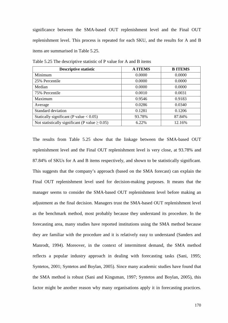
170
significance between the SMA-based OUT replenishment level and the Final OUT
replenishment level. This process is repeated for each SKU, and the results for A and B
items are summarised in Table 5.25.
Table 5.25 The descriptive statistic of P value for A and B items
Descriptive statistic A ITEMS B ITEMS Minimum 0.0000 0.0000 25% Percentile 0.0000 0.0000 Median 0.0000 0.0000 75% Percentile 0.0010 0.0031 Maximum 0.9546 0.9183 Average 0.0286 0.0340 Standard deviation 0.1281 0.1206 Statically significant (P value < 0.05) 93.78% 87.84% Not statistically significant (P value ≥ 0.05) 6.22% 12.16%
The results from Table 5.25 show that the linkage between the SMA-based OUT
replenishment level and the Final OUT replenishment level is very close, at 93.78% and
87.84% of SKUs for A and B items respectively, and shown to be statistically significant.
This suggests that the company’s approach (based on the SMA forecast) can explain the
Final OUT replenishment level used for decision-making purposes. It means that the
manager seems to consider the SMA-based OUT replenishment level before making an
adjustment as the final decision. Managers trust the SMA-based OUT replenishment level
as the benchmark method, most probably because they understand its procedure. In the
forecasting area, many studies have reported institutions using the SMA method because
they are familiar with the procedure and it is relatively easy to understand (Sanders and
Manrodt, 1994). Moreover, in the context of intermittent demand, the SMA method
reflects a popular industry approach in dealing with forecasting tasks (Sani, 1995;
Syntetos, 2001; Syntetos and Boylan, 2005). Since many academic studies have found that
the SMA method is robust (Sani and Kingsman, 1997; Syntetos and Boylan, 2005), this
factor might be another reason why many organisations apply it in forecasting practices.

171
The SMA-based OUT replenishment level is based on the forecasting result calculated
using the SMA method. The robustness of the SMA forecasting method, and its simplicity,
may explain the power of the SMA-based OUT replenishment level. Similarly, the case
organisation takes this approach as the benchmark method and seems to rely on it in
making the final decision. This can be the answer to our research question in terms of the
explanatory power of the SMA-based OUT replenishment level over the Final OUT
replenishment level.
5.13. Framework for judgmentally adjusted orders
Following from the discussion conducted in the previous sections, a framework is
presented below to facilitate the process of judgemental interventions in an inventory
control system. Base on the analysis we recommend the adjustment framework for
replenishment order decision which can be seen in Figure 5.19.
The first step of the process is to define the demand series characteristics (separate for
example between fast and intermittent demand) that consequently will necessitate a
different inventory policy. The policy itself will determine when and how much (time and
quantity related requirements) to order. This is essentially the principle of inventory system
regardless of whether adjustments are performed or not. The next step is to define the size
and sign of the judgemental adjustment. This should be based on two factors. First, we
have to consider any contextual information related to future events that may affect the
demand, such as the promotion of new product. Second, we need to analyse any archived
justifications of previous adjustments along with the performance of such adjustments in
order to be able to judge on the effects and performance of previous interventions. Well
documented and detailed justifications may enable managers to improve the performance
of future interventions. In this study, we have found that SKUs associated with a higher

172
number of justifications did relate to a better performance as compared to SKUS where
fewer justifications were offered. Moreover, we have found that negative and large
adjustment performed better than positive and small adjustment. Thus, in order to adjust
the replenishment orders, particularly when small and positive adjustments are regularly
taking place, we suggest to manager to give excessive consideration on the above factors.
In order to evaluate whether or not the adjustments may improve the performance of the
inventory system, the measurement procedure (i.e. what constitutes good performance) has
to be defined. We recommend that performance measurement is undertaken regularly. This
would facilitate the process of providing feedback in order to further improve the process
of judgemental interventions.
Figure 5.19 A framework to facilitate the process of judgemental adjustments
Archive justifications
Contextual information of future events
Define demand series characteristics
Define replenishment order procedure
Define the sign/size of adjustments
Define the measurement procedure of inventory system performance
Provide feedback for improving the process
(learning effect)

173
5.14. Conclusions
In this chapter, the empirical data analysis is discussed and the findings along with the
insights for real world practices are presented. In total, 359 A-class and 1,454 B-class
SKUs are considered for the purposes of this research. To develop an understanding of the
nature of the demand and its characteristic, the analysis of demand descriptive statistics is
conducted (in section 5.1) by considering demand per period, demand sizes, and inter-
demand intervals of each SKU. The results of the analysis show that the demand sizes for
A items are higher than for the B items, whereas the inverse is true with regards to the
inter-demand interval. Moreover, the analysis of the price of the SKUs is also carried out
in section 5.2, where we found that the range of prices for the B items is wider than that
related to the A items. It also found that B items are associated with high prices. From
above findings, we surmise that, although A-class items defined as the most important
SKU category (based on the ABC classification approach), B items also need more
attention from managers since this category, in this case organisation, is more intermittent
in nature, resulting presumably in higher obsolescence and having a much greater impact
on stock stock-holding costs.
The analyses have also been conducted on the adjustment distribution of the signed size of
adjustments, absolute size of adjustments, relative signed size and relative absolute size,
and found that adjustments may be fitted by some theoretical statistical distributions (see
section 5.3). The information that we obtained from the distribution of adjustments (form
and parameters) may be used as the control parameter (a minimum and a maximum
allowance) when managers make an adjustment. This is also an important finding for the
design of decision support systems.
Moreover, in analysis of the justification of adjustments presented in section 5.4, we have
attempted to cluster all the justifications into conceptually uniform categories, resulting in

174
24 such categories. We found that managers claimed a ‘decreasing demand’ situation in the
great majority of cases. This indicates that managers are indeed aware of important
contextual information, but for convenience they always report the same justification. In
addition, we found that the reasons for adjustments of the OUT level are mainly based on
the information that the manager has regarding demand for spare parts, inventory position,
or replenishment orders information, but are not based on the price of parts. Further, there
is often a discrepancy between the sign of the adjustments and what the demand patterns
indicate. The manager’s decision to change the OUT level does not always reflect demand
pattern changes. These findings indicate that managers still seem to make significant errors
in making adjustments in inventory control decisions and in adjusting the OUT level.
Adjustments are made in an arbitrary way and often reflect a sense of ownership on the
part of managers.
Simulation experiments were conducted to evaluate the performance of the inventory
system. The effect of adjustments was measured by reporting the implied inventory
investment, the Cycle Service Level (CSL) and fill rate achieved. We consider the System
OUT replenishment level (unadjusted OUT level), the Final OUT replenishment level
(adjusted OUT level), and the SMA-Based OUT replenishment level. The simulation is
carried out for A and B items and two scenarios are designed. We can see from the
simulation results in section 5.5 that, although the effects are not significant enough to
improve the performance of the inventory system, human intervention seems to offer a
reasonable advantage in stock control decision making.
To obtain a better understanding of the effects of human judgement on the stock control
decision, we evaluate the issues regarding the sign and size of adjustments, the bias and the
learning effect on judgmentally adjusted stock control decision making (these analyses are
presented in sections 5.6, 5.7, 5.9, and 5.10). The findings synchronize with what is found
175
in the judgemental forecasting field where the negative and large adjustments seem to
perform better in improving the inventory performance than the positive and small
adjustments. Moreover, we also found that bias may be introduced into the entire observed
system (System OUT replenishment level, the Final OUT replenishment level, and the
SMA-Based OUT replenishment level) and the negative bias leads to better performance
than does the positive one. In terms of learning effects, since the high number of
adjustment categories did not improve the inventory performance, we conclude that there
is no learning effect in A items. On the other hand, there is an occurrence of learning
effects for B items. Furthermore, from the analysis of the combination methods of the OUT
replenishment level (averaging 50%-50% weight of the OUT level) we found that that the
combination method in stock control seems to improve the performance of the inventory
system (see section 5.11).
In the analysis of the effects of justification of adjustments on inventory performance (see
section 5.8) we found that the SKUs associated with more than 75% of justifications
produce the highest stock control performance. This indicates that offering the rationale
and reasons for making the adjustment, including its documentation, is an important factor
that helps the decision maker to make adjustments. The justification for adjustments should
be determined not only by when the decision maker makes an adjustment, but also by how,
presenting the reason why the judgement is incorporated into the decision.
In addition, we attempted to investigate the explanatory power of the SMA-Based OUT
replenishment order as the benchmark method utilized in this case organisation. The
analysis result suggests that the company’s approach (based on the SMA forecast) can
explain the Final OUT replenishment level used for decision-making purposes. It means
that the manager seems to consider the SMA-based OUT replenishment level before

176
making an adjustment as the final decision. Managers trust the SMA-based OUT
replenishment level, most probably because they understand its procedure.
Based on all the findings above, we develop a framework for judgementally adjusted
replenishment orders which is presented in Section 5.13.

177
Chapter 6. CONCLUSION, CONTRIBUTIONS, LIMITATIONS, AND FURTHER RESEARCH
6.1. Introduction
This chapter provides a brief discussion of the main issues addressed in our research. The
implications of this research for the OM theory and practice are also presented. Moreover,
the limitations of this research, theoretically and empirically, are identified and the next
steps of the research are suggested.
This study aimed to explore the effects of incorporating human judgement into inventory
decision-making.
The aim of the research was reflected in the following objectives:
1. To critically review the literature on how judgement relates to the main functions of
an inventory system: demand categorisation, forecasting and stock control (Chapters 2
and 3).
2. To assess the implications of judgemental adjustments on real data, focusing on
replenishment orders (Chapters 4 and 5).
3. To link the performance of adjustments with the managers’ justification for
introducing such adjustments in the first place (Chapter 5).
4. To understand for the first time how managers adjust inventory-related decisions
(Chapters 4 and 5).

178
5. To evaluate the circumstances under which human judgement leads to performance
improvement (Chapter 5).
6. To derive a number of insights with regard to practical applications and a number of
suggestions for improving the functionality of software packages (Chapter 5).
All the objectives have been achieved and the summary and contributions of the thesis are
outlined in the following section.
6.2. Conclusions
Physical inventories constitute a considerable proportion of companies’ investments in
today’s competitive environment. The trade-off between customer service levels and
inventory investments is addressed in practice by formal quantitative inventory
management (stock control) solutions. The solutions need to be fully automated since,
commonly, organizations deal with a tremendous number of SKUs. From the literature
review we found that decision makers/managers tend to reflect (superimpose) their own
judgment on the solutions resulted from specialized software systems.
This study was carried out in a single company representing the European logistics
headquarters of a major international electronics manufacturer. In this research we are
concerned with the value being added (or not) when statistical/quantitative output is
judgementally adjusted by managers. Our work aims to investigate the effects of
incorporating human judgement into such inventory-related decisions. In achieving the
aim, first, a set of relevant research questions was developed based on a critical review of
the literature. Then, an extended database of approximately 1,800 SKUs from the case
study organisation was analysed for the purpose of addressing these research questions. In
addition to exploratory empirical analysis, a simulation experiment was performed to

179
evaluate in a dynamic fashion the effects of adjustments on the performance of a stock
control system.
A computer simulation experiment was designed to quantify the inventory performance
and evaluate the implications of judgemental adjustments in an inventory system, focusing
on replenishment orders. For simulation purposes, the database was arranged in Microsoft
Excel worksheets and then Visual Basic Application code was developed to measure
inventory performance. The results on the simulation experiment revealed that, by
considering the trade-off between inventory cost and service level, it seems that
judgemental adjustments account for an improvement in inventory investment. However,
the effects are not too prevailing in increasing the CSL and fill rate. Overall, the results
indicate that human intervention seems to offer a ‘reasonable’ advantage in stock control
decision making, important enough to offer a justification for these interventions in the
first place. This result is in line with the previous empirical research in the area of demand
forecasting conducted by Syntetos et al. (2009b) and Syntetos et al. (2010a) which shows
that the inventory implications of adjusting demand forecasts are prominent. Moreover, the
outcome of our empirical research shows (indirectly) that the effect of adjusting inventory
decisions is less significant than that associated with adjusting forecasts. This finding
confirms the previous study conducted by Syntetos et al. (2011) about the comparatively
bigger importance of adjusting at the forecasting rather than at the inventory control level.
With regards to the characteristics of the adjustments, we have found that negative
adjustments result in better performance than positive ones, and that adjustments of a
medium/large size perform better than small ones. This is aligned with the main
conclusions derived in the forecasting literature and it can similarly be explained in terms
of: i) a sense of ownership associated with small adjustments, that do not necessarily
reflect an important piece of information but rather a desire to merely intervene in the

180
system; ii) the optimistic bias characterizing many individuals that leads to upward
(positive) adjustments. Negative adjustments would typically result in a reduction of the
service provision if things were not to change, so adjustments in that direction should
typically be associated with some genuine knowledge about the underlying demand
process. We have also explored this bias-related properties of judgemental adjustments and
have found that indeed bias may be present in such a system. Furthermore, negative bias
leads to better performance than positive. This indicates that, if the managers adjust the
Order-Up-To (OUT) levels without any logical justification, the downward adjustments
would seem to perform better than the upward ones. Some learning effect seems to take
place in the process of adjusting stock control quantities, as it was found that SKUs
associated with a high number of adjustments are indeed also associated with a better
inventory control performance.
Since the justification of the adjustments was recorded, we attempted to assess whether
offering a justification is associated with better performance. The association of
judgemental adjustments with a justification provided can be viewed as a contribution in
its own right, as no empirical studies have been previously conducted in this area, neither
in the forecasting nor in the stock control field. From the simulation experiment results, we
found that providing a justification for adjusting stock control quantities may lead to an
improvement in inventory performance.
Justifications very often related to a perceived change in the underlying demand pattern,
(recorded as ‘demand increasing’ or ‘decreasing’). An examination of the consistency
between such justifications and the actual underlying demand movement was undertaken
and it was found that in about 21% and 25% of the cases for A and B items respectively,
adjustments were made in a different direction from that of the time series evolution. This
indicates that managers may make significant errors in adjusting the OUT levels. They

181
seem to make judgements in an arbitrary way, often reflecting the managers’ sense of
ownership. We clustered the justifications into 24 conceptually uniform categories, of
which the ‘decreasing demand’ category accounted for 40.9% and 45.5% for the A- and B-
class items. Also, we found that most of the reasons for adjustments made by the managers
are merely related to the information that the managers have to hand, regarding the demand
for spare parts, their inventory position, and/or replenishment order information, but not
upon the prices of spare parts.
An analysis of combined methods (the combination of System OUT replenishment level
and Final OUT replenishment level, System OUT replenishment level and SMA-based
OUT replenishment level, and Final OUT replenishment level and SMA-based OUT
replenishment level) for calculating the inventory performance was also conducted. The
combination value was calculated by averaging (50%-50% weight) the OUT replenishment
level resulting from each method. The findings indicate that the combined method of stock
control seems to improve the performance of the inventory system, especially in reducing
inventory investment. However, other additional combination methods need to be carried
out in order to achieve a better understanding of this issue.
In making adjustments to the final decision of the replenishment order quantity, managers
use the SMA-based OUT replenishment levels as their benchmark. By using regression
analysis we find that the SMA-based OUT replenishment level (that is based on the SMA
forecast) can explain the Final OUT replenishment level. This indicates that managers trust
this method and rely on it in making the final decisions.
From the empirical analysis we found some theoretical distributions that fit the
adjustments. The goodness-of-fit of theoretical statistical distributions on judgemental
adjustments was analysed using the Kolmogorov-Smirnov (K-S) test. The results can be
seen in Table 5.5. For the A items it is found that the Cauchy distribution provides a strong

182
fit for most series of signed sizes of adjustments (80.0 %) and relative signed sizes of
adjustments (83.8%), whereas the Gamma distribution provides a strong fit for the absolute
size of adjustments (76.3%) and the relative absolute size of adjustments (88.8%). Similar
results are reported for the B items, where the Cauchy is associated with a strong fit for
95.0% of the relative signed size of adjustments and the relative absolute size of
adjustment (95.0%). The Gamma distribution offers a strong fit for the absolute size of
adjustments (97.5%), whereas the Weibull distribution performs very well on the signed
size of adjustments (95.0% cases of strong fit).
Knowing the distribution that resembles the range and shape of the relevant decisions
made by humans is most important in terms of the design of support systems. A support
system is any structured process that may facilitate decision making. It may be a well
documented process, but mostly nowadays is a computerised solution (i.e. software
package). A software package which is developed to support the inventory management
function is called an Inventory Support System (ISS). ISS has not been discussed in the
literature. From the goodness-of-fit tests, some theoretical distributions that fit the
adjustment distributions were found. Based on that information, managers may define a
specific percentile above or below which adjustments are permitted. For example, as we
found that small adjustments are not performing well, managers may decide that there is no
adjustment allowed below the fifth percentile. Moreover, since large adjustments are found
to perform well, perhaps managers may want to have more information on the rationale
behind large adjustments (exceeding say the 90th percentile).
Based on the above findings obtained through the empirical analysis, we can make a
number of suggestions (see Figure 5.19) for improving the functionality of software
packages.

183
6.3. Implications
This research has generated a number of implications for the OM theory and practice.
More specifically, it has contributed to the development of insights in managing
intermittent demand inventories.
6.3.1. Implications for the OM theory
This research is the first study that investigates in an empirical way the effects of
judgementally adjusting replenishment decisions. It analyses the way adjustments are made
by humans and their effect on the performance of a stock control system in the context of
intermittent demand. There is a substantial body of knowledge on the effects of judgment
in the forecasting area, particularly on demand/sales forecasting. When it comes to the
inventory area though there are only two studies that look at this issue. The first one is a
presentation in the International Symposium of Forecasting by Kolassa et al. (2008) that
offers some very preliminary empirical insights into this issue. The second is a study
conducted by Syntetos et al. (2011) that relies upon the use of System Dynamics. There are
no complete studies to date that look, empirically, at the implications of human
interventions into an inventory system, particularly on replenishment order decisions. This
study points out the need for more empirical work (rather than laboratory experiments) in
the area of judgement and inventory control. It demonstrates the complications of real
world inventory systems and the non-textbook behavior of such systems (both in terms of
their actual operation and optimization) that call for more work with real data, and/or real
situations. We return to this issue when we discuss the next steps of research.
Moreover, the forecasting literature suggests that judgemental forecasting is most useful in
terms of potential amendments to Forecast Support Systems (FSS). For example, the study
by Fildes et al. (2009) and Syntetos et al. (2009b) found that small adjustments do not
perform well since they are known to simply reflect a response to noise, whereas the

184
negative adjustments perform better than the positive ones as they reflect genuinely
important information (Fildes et al., 2009). From the outcome of this research, a reference
may now be made to Inventory Support Systems (ISS). Similarly, to Forecast Support
Systems, systems that support the inventory function and provide guidance into how the
inventory replenishment task may be improved should attract high attention in the
academic community and research into both their functionality and implications for real
world practices.
In addition, since the justifications of adjustments are provided by the case organisation,
this research investigates the performance of stock control systems when justification of
adjustments is offered as compared to those without a justification. This is also the first
study that explicitly analyses in an empirical way the justification for adjustments. There is
no previous study has discussed this issue, not only in the area of inventory, but in the area
of forecasting as well.
Finally, since this research includes elements of Operation Management (OM)/Operational
Research (OR) and behavioral aspects of decision making, it should contribute and
advance knowledge in the field of behavioral operations.
6.3.2. Implications for the OM practice
This research provides the evidence of what is a standard practice in inventory systems
where managers tend to adjust replenishment order decisions. As discussed before, there
are only two studies (Kolassa et al., 2008 and Syntetos et al., 2011) investigating the
effects of such adjustments and no empirical evidence has been put forward thus far in the
literature with regards to this issue. The current research documented the process of
adjusting the replenishment order decision as a standard practice in the real inventory
world.

185
Furthermore, this research has some implications for the statistical analysis of the
properties of the adjustments (i.e. formal distributions that fit the adjustments). The results
of empirical analysis of this research may lead towards the improvement of the
functionality of software packages, and further towards the development of more generic
ISS.
These implications can be summarised on the following issues:
• Defining the demand series characteristics for the purpose of choosing an appropriate
inventory policy. The policy itself will determine when and how much (time and
quantity related requirements) to order.
• Deciding the size and sign of the judgemental adjustment. In this research, we found
that the negative and adjustments perform better in improving the performance of the
inventory system compared to the positive and small adjustments. The size of
adjustments may be defined by using the parameters of the particular distributions that
provide a good fit to the adjustments. For example, by knowing the mean and the
variance of such distribution, managers may decide the specific percentile
above/below which adjustments need to be authorized/or further debated.
• Considering any contextual information related to future events that may affect the
demand, such as the promotion of new product in deciding the size and sign of
adjustments.
• Evaluating any archived justifications of previous adjustments along with the
performance of such adjustments is also important in order to review the effects and
performance of previous interventions. Well-documented and detailed justifications
may enable managers to improve the performance of future interventions.
• In order to evaluate whether or not the adjustments may improve the performance of
the inventory system, the measurement procedure (i.e. what constitutes good

186
performance) has to be defined. We recommend that performance measurement is
undertaken regularly. This would facilitate the process of providing feedback in order
to further improve the process of judgemental interventions.
6.4. Limitations
In this section we summarise the limitations of the work conducted for the purposes of this
research.
6.4.1. Generalisation of theory
The analysis in this research has been developed for a specific case originated from one
organisation. As discussed in Chapter 1, the fact that this work is based on a single case
can be justified by the lack of any previous research in this area, and even more so by the
sensitivity of the information required in conducting such a study. Specificities related to
the problem in hand may obviously differ from one situation to the other and in that respect
generality may be questioned. Although we are concerned with a single organisation and
essentially a particular case of SKUs (spare/service parts), this company could be viewed
as a ‘good sample’ to be used for discussing the pertinent issues. First of all the demand for
spare parts is predominantly intermittent in nature and intermittent demand patterns prevail
in any organisational setting. In fact the vast majority of SKUs in any business setting are
intermittent in nature. Second, and very importantly, we cover SKUs from two classes in
an ABC classification by value and that also covers a big part of any company's investment
in stock. Finally the company's practices are very typical (to the best of our knowledge) of
what is happening in industry. That is people do not adjust replenishment orders (order
quantities) but order levels (re-order points or Order-Up-To levels).
The general observations and associated learning should easily be transferred to other
organisations as well. Moreover, the insights and discussions regarding the judgementally

187
adjusted stock control decisions in this research should provide practical insights to many
other industrial organisations. However, replications of our research on more cases
definitely need to be conducted for the purpose of obtaining a better understanding of all
pertinent issues.
6.4.2. Interviews with the manager
This research does not involve the collection of any qualitative information directly from
the managers who conducted the actual judgemental adjustments. Interviews with these
people would enable an understanding on ‘how’ and ‘why’ adjustments are performed.
Further, they would also allow a direct linkage of such information with the quantitatively
derived insights of our research and the actual performance of the adjustments. To the best
of our knowledge, the linkage identified above is a missing one also in the forecasting, not
only in the inventory control, literature.
6.4.3. Construction of the database and simulation experiment
A database was established in order to conduct the simulation experiment. In the process of
construction (explained in section 4.3), the Visual Basic software (embedded in Microsoft
Excel) was used. However, some steps of the process had to be done manually, for
example entering all SKUs for every period in a single Excel worksheet (one SKU per
row). This process might have been more effective and efficient if the VBA software had
been used. Moreover, the simulation experiment looks only at one forecasting model, that
is, a simple moving average. Although much of the academic literature states that this
forecasting method is robust, several forecasting procedures are more suitable for
intermittent demand, such as Croston’s method and the SBA (Syntetos-Boylan
Approximation, Syntetos and Boylan, 2005.

188
6.4.4. Goodness-of-fit distribution tests
The Kolmogorov-Smirnov (K-S) test was deployed to determine the goodness-of-fit of the
adjustments distributions, in Chapter 5. However, this test is not ideal since it relies upon
continuous random variables to be tested. On the other hand, the sign and size of
adjustments constitute the random variables in our analysis. These are discrete variables,
since the value could be any integer between zero and plus infinity, and it conflicts with
the theoretical cumulative distribution being tested in K-S. However, as pointed out in
section 5.3, the K-S test was chosen as there is no requirement for grouping the data into
categories, and it seems flexible. In addition, no more than two parameter statistical
distributions were considered in our analysis.
6.5. Further research
Future steps of the research are intended to:
• Replicate the analysis in other datasets/organisations. As discussed above, empirical
analysis on one case study seems insufficient for the generalisation of the concepts and
the outcomes of this research. An extensive study of several cases in other
organizations needs to be undertaken where human intervention is incorporated in
stock control decision making. In addition, in order to further understand and clarify
‘how’ and ‘why’ managers perform adjustments in stock control, interviews are also
highly recommended.
• Develop more suitable scenarios using more appropriate forecasting methods such as
the SBA and stock control policies to investigate the effects of human intervention in
an inventory control setting. Moreover, the study of a system where adjustments are
performed at both the forecasting and inventory control stage, would allow developing

189
our empirical understanding on the progressive accumulation of the effects of
adjustments in an inventory management context.
• Develop a Decision Support System (DSS) for stock control purposes (what may be
termed as Inventory Support System - ISS). So far, to the best of our knowledge, there
is not a single academic publication that discusses the features of computerized support
systems for facilitating judgemental adjustments of inventory related decisions. Given
the extent to which managers intervene into inventory applications, such a support
system would be very welcomed by practitioners.
190
BIBLIOGRAPHY
Aberdeen Group (2005). The Service Parts Management Solution Selection Report, SPM
Strategy and Technology Selection Handbook, Aberdeen Group, Boston, MA. Adenso-Diaz, B., Moreno, P., Gutierrez, E., and Lozano, S. (2012). An analysis of the
main factors affecting bullwhip in reverse supply chains. International Journal of Production Economic, 135, 917-928.
Alamri, A. A. and Balkhi, Z. T. (2007). The effects of learning and forgetting on the
optimal production lot size for deteriorating items with time varying demand and deterioration rates. International Journal of Production Economics, 107, 125-138.
Amoako-Gyampah, K. and Meredith, J. R. (1989). The operations management research
agenda: an update. Journal of Operations Management, 8, 250-262. Ancarani, A., Di Mauro, C., and D’Urso, D. (2013). A human experiment on inventory
decisions under supply uncertainty. International Journal of Production Economics, 142, 61-73.
Anderson Jr, E. G. and Morrice, D. J. (2000). A simulation game for teaching service-
oriented supply chain management: does information sharing help managers with service capacity decisions?. Production and Operations Management, 9, 40-55.
Angus-Leppan, P. and V. Fatseas. (1986). The forecasting accuracy of trainee accountants
using judgemental and statistical techniques. Accounting and Business Research, 16, 179-188.
Archibald, B. C. and Silver, E. A. (1978). (s, S) policies under continuous review and
discrete compound Poisson demand. Management Science, 24, 899-909. Armstrong, J. S. (1988). Research needs in forecasting. International Journal of
Forecasting, 4, 499-465. Babai, M. Z., Jemai, Z., and Dallery, Y. (2011). Analysis of order-up-to level inventory
systems with compound Poisson demand. European Journal of Operational Research, 210, 552-558.
Beach, R., Muhlemann, A. P., Price, D. H. R., Paterson, A., and Sharp, J. A. (2001). The
role of qualitative methods in production management research. International Journal of Production Economics, 74, 201-212.
Bendoly, E., Donohue, K., and Schultz, K. L. (2006) Behavior in operations management:
Assessing recent findings and revisiting old assumptions. Journal of Operations Management, 24, 737-752.
191
Bolger, F., and Wright, G. (1994). Assessing the quality of expert judgment: Issues and analysis. Decision Support Systems, 11, 1-24.
Bonney, M. C. and Jaber, M. Y. (2011). Environmentally responsible inventory models:
Non-classical models for a non-classical era. International Journal of Production Economics, 133, 43-53.
Bookbinder, J. H. and Lordahl, A. E. (1989). Estimation of inventory re-order levels using
the bootstrap statistical procedure. IIE transactions, 21, 302-312. Boylan, J. E. and Johnston, F. R. (2003). Optimality and robustness of combinations of
moving averages. Journal of the Operational Research Society, 54, 109-115. Boylan, J. E. and Syntetos, A. A. (2007). The accuracy of a modified Croston procedure.
International Journal of Production Economics, 107, 511-517. Boylan, J.E., Syntetos, A.A., and Karakostas, G. C. (2008). Classification for forecasting
and stock control: a case study. Journal of Operational Research Society, 59, 473. Bryman, A. (2008). Social Research Methods, 3rd Edition, Oxford University Press,
Oxford. Bryman, A. and Bell, E. (2011). Business Research Methods, 3rd Edition, Oxford
University Press, Oxford. Bunn, D. and Wright, G. (1991). Interaction of judgemental and statistical forecasting
methods: issues and analysis. Management Science, 37, 501-518. Burgin, T. A. (1975). The gamma distribution and inventory control. Operational Research
Quarterly, 507-525. Buzacott, J.A. (1999). Dynamic inventory targets revisited. Journal of the Operational
Research Society, 50, 697-703. Carbone, R., Anderson, A., Corriveau, Y., and Corson, P. P. (1983). Comparing for
different time series methods the value of technical expertise, individual analysis, and judgemental adjustment. Management Science, 29, 559-566.
Carbone, R. and Gorr, W. L. (1985). Accuracy of Judgemental Forecasting of Time Series.
Decision Science, 153-160. Carlson, J. G. and Rowe, A. J. (1976). How much does forgetting cost? Industrial
Engineering, 8, 40-47. Carter, C. R., Kaufmann, L., and Michel, A. (2007). Behavioural supply management: a
taxonomy of judgement and decision-making biases. International Journal of Physical Distribution & Logistic Management, 37, 631-669.
Cerullo, M. J. and Avila, A. (1975). Sales forecasting practices: a survey. Managerial
Planning, 24, 33-39.

192
Chaharsooghi, S. K., Heydari, J., and Zegordi, S. H. (2008). A reinforcement learning
model for supply chain ordering management: An application to the beer game. Decision Support Systems, 45, 949-959.
Chen, I. J. (2001). Planning for ERP systems: analysis and future trend. Business Process
Management Journal, 7, 374-386. Chen, Y., Li, K.W., Kilgour, D.M., and Hipel, K.W. (2008). A case-based model for multi-
criteria ABC analysis. Computers & Operations Research, 35, 776-96. Chikán, A. (2001). Integration of production and logistics in principle, in practice and in
education. International Journal of Production Economics, 69, 129-140. Chikán, A. (2007). The new role of inventories in business: Real world changes and
research consequences. International Journal of Production Economics, 108, 54-62. Chikán, A. (2009). An empirical analysis of managerial approaches to the role of
inventories. International Journal of Production Economics, 118, 131-135. Chung, S. H., and Snyder, C. A. (2000). ERP adoption: a technological evolution
approach. International Journal of Agile Management Systems, 2, 24-32. Clement, R. (1989). Combining forecasts: a review and annotated bibliography.
International Journal of Forecasting, 5, 559-583. Collis, J. and Hussey, R. (2009). Business research: A practical guide for undergraduate
and postgraduate students, 3rd Edition, Palgrave Macmillan, London. Collopy, F. and Armstrong, J. S. (1992). Expert opinions about extrapolation and mystery
of the overlooked discontinuities. International Journal of Forecasting, 8, 575-582. Cooper, D. R., & Schindler, P. S. (2002). Business Research Methods. 8th edition.
McGrawHill Costantini, M. and Pappalardo, C. (2010). A hierarchical procedure for the combination of
forecasts. International Journal of Forecasting, 26, 725-743. Croson, R. and Donohue, K. (2006). Behavioral causes of the bullwhip effect and the
observed value of inventory information. Management Science, 52, 323-336. Croson, R., Schultz, K., Siemsen, E., and Yeo, M. L. (2013) Behavioral operations: The
state of the field. Journal of Operations Management, 31, 1-5. Croston, J. D. (1972). Forecasting and stock control for intermittent demands. Operational
Research Quarterly, 289-303. Davidovitch, L., Parush, A. and Shtub, A. (2008). Simulation-based learning: The
learning–forgetting–relearning process and impact of learning history. Computers & Education, 50, 866-880.

193
Davydenko, A. and Fildes, R. (2013). Measuring forecasting accuracy: The case of
judgmental adjustments to SKU-level demand forecasts. International Journal of Forecasting, 29, 510-522.
Delhoum, S. (2008). Evaluation of the Impact of Learning Labs on Inventory Control-An
Experimental Approach with a Collaborative Simulation Game of a Production Network. GITO-Verlag. Berlin
Deloitte. (2006). The Service Revolution in Global Manufacturing Industries, Deloitte
Research, New York, NY. Denscombe, M. (2010). The Good Research Guide: for small-scale social research
projects, 4th Edition, Open University Press, Maidenhead. DFT, 2012, Waste Electrical and Electronic Equipment (WEEE). Available at:
http://www.dft.gov.uk/vca/enforcement/weee-enforcement.asp, accessed on: 3 December 2012
Diamantopoulos, A. and Mathews, B. (1989). Factors affecting the nature and
effectiveness of subjective revision in sales forecasting: An empirical study. Managerial and Decision Economics, 10, 51-59.
Easterby-Smith, M., Thorpe, R., and Lowe, A. (2004) Management Research: an
Introduction, 2nd Edition, Sage Publications Ltd, London. Eaves, A. H. C. (2002). Forecasting, Ordering and Stock-Holding for Erratic Demand.
Paper presented at the 21th International Symposium on Forecasting; 23-26 June 2002; Pine Mountain.
Eaves, A. H. C. and Kingsman, B. G. (2004). Forecasting for the ordering and stock-
holding of spare parts. Journal of the Operational Research Society, 55, 431-437. Edmundson, R. H. (1990). Decomposition: a strategy for judgemental forecasting,
International Journal of Forecasting. 9, 305-314. Efron, B. (1979). Bootstrap methods: another look at the jackknife. The annals of
Statistics, 7, 1-26. Elmaghraby, S. E. (1990). Economic manufacturing quantities under conditions of learning
and forgetting (EMQ/LaF). Production Planning Control, 1, 196-2008. Environement Agency. (2012). Waste electrical and electronic equipment (WEEE).
Available at: http://www.environment-agency.gov.uk/business/topics/waste/32084. aspx, access: 05 November 2012.
Eroglu, C. (2006). An Investigation of Accuracy, Learning and Biases in Judgemental
Adjustment of Statistical Forecasts. Dissertation, Ohio State University.

194
Eroglu, C. and Croxton, K. L. (2010). Biases in judgemental adjustments of statistical forecasts: The role of individual differences. International Journal of Forecasting, 26, 116–133.
Eurostat. (2012). Waste Electrical and Electronic Equipment (WEEE). Available at:
http://epp.eurostat.ec.europa.eu/portal/page/portal/waste/key_waste_streams/waste_electrical_electronic_equipment_weee, accessed on: 3 December 2012.
Fang, Y. (2003). Forecasting combination and encompassing tests. International Journal of
Forecasting, 19, 87-94. Fildes, R., Goodwin, P., and Lawrence, M. (2006). The design features of forecasting
support systems and their effectiveness. Decision Support Systems, 42, 351−361. Fildes, R., Goodwin, P., Lawrence, M., and Nikolopoulos, K. (2009). Effective forecasting
and judgemental adjustment: an empirical evaluation and strategies for improvement in supply-chain planning. International Journal of Forecasting, 25, 3-23.
Fildes, R., Nikolopoulos, K., Cronel, S. F., and Syntetos, A. A. (2008). Forecasting and
operational research: a review. Journal of the Operational Research Society, 59, 1150-1172.
Fisk, J. and Ballou, R. (1982). Production lot sizing under a learning effect. IIE
Transactions, 14, 257-264. Flores, B.E. and Whybark, D.C. (1987). Implementing multiple criteria ABC analysis.
Journal of Operations Management, 7, 79-85. Gargeya, V. B. and Brady, C. (2005). Success and failure factors of adopting SAP in ERP
system implementation. Business Process Management Journal, 11, 501 – 516 Gattiker, T. F. and Parente, D. H. (2007). Introduction to the special issue on innovative
data sources for empirically building and validating theories in operations management. Journal of Operations Management, 25, 957-961.
Goodwin, P. (2000a). Correct or combine? Mechanically integrating judgemental forecasts
with statistical methods. International Journal of Forecasting, 16, 261–275. Goodwin, P. (2000b). Improving the voluntary integration of statistical forecasts and
judgment. International Journal of Forecasting, 16, 85-99. Goodwin, P. (2005). How to integrate management judgmental with statistical forecasts.
The International Journal of Applied Forecasting, 1, 8–12. Goodwin, P. and Fildes, R. (1999). Judgemental forecasts of time series affected by special
events: Does providing a statistical forecast improve accuracy?. Journal of Behavioral Decision Making, 12, 37-53.
Goodwin, P., Fildes, R., Lawrence, M., and Nikolopoulos, N. (2006). The process of using
a forecasting support system. Working Paper Series. University of Bath.

195
Goodwin, P., Fildes, R., Lawrence, M., and Stephens, G. (2011). Restrictiveness and
guidance in support systems. The International Journal of Management Science, 39, 242-253.
Goodwin, P. and Wright, G. (1993). Improving judgemental series forecasting: A review
of the guidance provided by research. International Journal of Forecasting, 9, 147-161.
Goodwin, P. and Wright, G. (1994). Heuristics, biases and improvement strategies in
judgmental time series forecasting. The International Journal of Management Science, 22, 553-568.
Gutierrez, R.S., Solis, A.O., and Mukhopadhyay, S. (2008). Lumpy demand forecasting
using neural networks, International Journal of Production Economics, 111, 409-20. Hanke, J. E. And Wichern, D. W. (2009). Business Forecasting, 9th Edition, Pearson
Education, Jew Jersey. Harvey, N. and Fischer, I. (1997). Taking advice: Accepting help, improving judgment,
and sharing responsibility. Organizational Behavior and Human Decision Processes, 70, 117-133.
Harvey, D. S., Leybourne, S. J., and Newbold, P. (1998). Tests for forecast encompassing.
Journal of Business & Economic Statistics, 16, 254-259. Heinecke, G., Syntetos, A.A., and Wang, W. (2013). Forecasting-based SKU
classification. International Journal of Production Economics, 143, 455-462. Hibon, M. and Evgeniou, T. (2005). To combine or not to combine: selecting among
forecasts and their combinations. International Journal of Forecasting, 21, 15-24. Hussey, J. and Hussey, R. (1997) Business Research: a practical guide for undergraduate
and postgraduate students. Palgrave, New York. Ibrahim, A. (2007). Soft Enterprise Resource Planning (ERP) Implementation Related
Factors: A Case Study Strategy. Unpublished Ph.D. thesis. University of Salford, Manchester. UK.
Jaber, M. Y. and Bonney, M. (1996a). Production breaks and the learning curve: The
forgetting phenomenon. Applied Mathematical Modelling, 20, 162-169. Jaber, M. Y. and Bonney, M. (1996b). Optimal lot sizing under learning considerations:
The bounded learning case. Applied Mathematical Modelling, 20, 750-755 Jaber, M. Y. and Bonney, M. (1997). A comparative study of learning curves with
forgetting. Applied Mathematical Modelling, 21, 523-531. Jaber, M. Y. and Bonney, M. (2003). Lot sizing with learning and forgetting in set-ups and
in product quality. International Journal of Production Economics, 83, 95-111.

196
Jaber, M. Y., Goyal, S. K., and Imran, M. (2008). Economic production quantity model for
items with imperfect quality subject to learning effects. International Journal of Production Economics, 115, 143-150.
Jaber, M. Y. and Guiffrida, A. L. (2004). Learning curves for imperfect production
processes with reworks and process restoration interruptions. European Journal of Operational Research, 189, 93-104.
Jaber, M. Y. and Guiffrida, A. L. (2008). Learning curves for processes generating defects
requiring reworks. European Journal of Operational Research, 159, 663-672. Jacob, F. R. and Weston Jr., F.C. (2007). Enterprise resource planning (ERP) – a brief
history. Journal of Operations Management. 25, 357-363. Jasper, J. B. (2006). Quick Response Solutions, FedEx Critical Inventory Logistics
Revitalized, FedEx, Memphis, TN. Jenks, J. M. (1983). Non-computer Forecasts to Use Right Now. Business Marketing, 69,
82-84. Johnston, F. R., and Boylan, J. E. (1996). Forecasting for items with intermittent demand.
Journal of the Operational Research Society, 113-121. Johnston, F. R., Boylan, J. E., Meadows, M., and Shale, E. (1999). Some properties of a
simple moving average when applied to forecasting a time series. Journal of the Operational Reserach Society, 50, 1267-1271.
Klassen, R. D. and Flores, B. E. (2001). Forecasting practices of Canadian Firms: Survey
results and comparison. International Journal of Production Economics, 70, 163-174.
Klein, H. E. and Linneman, R. E. (1984). Environmental assessment: An international
study of corporate practice. Journal of Business Strategy, 5, 66-75. Kolassa S., Schütz W., Syntetos A. A., and Boylan, J. E. (2008). Judgemental changes to
retail sales forecasts and automatic orders. Paper presented at the 28th International Symposium on Forecasting; 22-25 June 2008; Nice, France.
Kostenko, A. V. and Hyndman, R. J. (2006). A note on the categorization of demand
patterns. Available at: http://www-personal.buseco.monash.edu.au/~hyndman/ papers/idcat.pdf, accessed on: 15/05/2012
Law, A. M. (1991). Simulation model's level of detail determines effectiveness. Industrial
Engineering, 23, 16-18. Lawrence, M. J., Edmundson, R. H., and O’Connor, M. J. (1986). The accuracy of
combining judgemental and statistical forecasts. Management Science, 32, 1521-1532.

197
Lawrence, M., and O’Connor, M. (2005). Judgemental forecasting in the presence of loss functions. International Journal of Forecasting, 21, 3-14.
Lawrence, M., Goodwin, P., O’Connor, M., and Onkal, D. (2006). Judgemental
forecasting: A review of progress over the last 25 years. International Journal of Forecasting, 22, 493-518.
Lee, W. Y., Goodwin, P., Fildes, R., Nikolopoulos, K., and Lawrence, M. (2007).
Providing support for the use of analogies in demand forecasting tasks. International Journal of Forecasting, 23, 377–390
Leitner, J. and Leopold-Wildburger, U. (2011). Experiments on forecasting behavior with
several sources of information–A review of the literature. European Journal of Operational Research, 213, 459-469.
Lengu, D. (2012). Modelling and Prediction of Intermittent Demand Distributions.
Unpublished Ph.D. thesis. University of Salford, Manchester. UK. Leon, A. (2008). Enterprise Resource Planning. Tata McGraw-Hill. New Delhi: India. Levén, E. and Segerstedt, A. (2004). Inventory control with a modified Croston procedure
and Erlang distribution. International Journal of Production Economics, 90, 361-367.
Levitt, B. and March, J.G. (1996). Organizational learning. In M.D. Cohen and L.S.
Sproull (Eds) Lim, J. S. and O’Connor, M. (1996). Judgemental forecasting with time series and causal
information. International Journal of Forecasting, 12, 139-153. Lincoln, Y.S. and Guba, E. G. (1985). Naturalistic Inquiry. Sage, California. Mabert, V. A., Soni, A., and Venkataramanan. (2003). The impact of organization size on
enterprise resource planning (ERP) implementations in the US manufacturing sector. The International Journal of Management Science, 31, 235-246.
Makridakis, S. (1989). Why combining works? International Journal of Forecasting, 5,
601-603. Makridakis, S., Andersen, A., Carbone, R., Fildes, R., Hibon, M., Lewandowski, R.,
Newton, J., Parzen, E. and Winkler, R. (1982). The accuracy of extrapolation (time series) methods: Results of a forecasting competition. International Journal of Forecasting, 1, 111-153.
Makridakis, S. and Hibon, M. (1979). Accuracy of forecasting: an empirical investigation
(with discussion). Journal of the Royal Statistical Society, 142, 97–145. Makridakis, S., Hibon, M., and Moser, C. (1979). Accuracy of forecasting: An empirical
investigation. Journal of the Royal Statistical Society. Series A (General), 97-145.

198
Makridakis, S. G., & Wheelwright, S. C. (1989). Forecasting methods for management, 5th Edition, John Wiley & Sons.
Makridakis, S., Wheelwright, S. C., and Hyndman, R. J. (1998). Forecasting Methods and
Applications, 3rd Edition, John Wiley & Sons Inc, New Jersey. Martin, H., Syntetos, A. A., Parodi, A., Polychronakis, Y. E., and Pintelon, L. (2010)
Integrating the spare parts supply chain: an inter-disciplinary account. Journal of Manufacturing Technology Management, 21, 226-245.
Matheus, P. and Gelders, L. (2000). The (R,Q) inventory policy subject to a compound
Poisson demand pattern. International Journal of Production Economics, 68, 307-317.
Mathew, B. P. and Diamantopoulos, A. (1986). Managerial intervention in forecasting: An
empirical investigation of forecast manipulation. International Journal of Research in Marketing, 3, 3-10.
Matthew, B. P. and Diamantopoulos, A. (1989). Judgemental revision of sales forecasts: A
longitudinal extension. International Journal of Forecasting, 8, 129-140. Matthew, B. P. and Diamantopoulos, A. 1990. Judgemental revision of sales forecasts:
effectiveness of forecast selection. International Journal of Forecasting, 9, 407-415. Mathew, B. P., and Diamantopoulos, A. (1992). Judgmental revision of sales forecasts-the
relative performance of judgementally revised versus non revised forecasts. International Journal of Forecasting, 11, 569–576.
McCarthy, T. M., Davis, D., Golic, S., and Mentzer, J. (2006). The evaluation of sales
forecasting management: a 20-year longitudinal study of forecasting practices. International Journal of Forecasting, 25, 303-324.
Mendelson, H. (2000). ERP: Overview. Available at: faculty.ist.psu.edu/yen/421/erp.pdf,
accessed on: 05 November 2012. Miles, M.B. and Hurberman, A.M. (1994). Qualitative Data Analysis, 2nd Edition, Sage
Publications, London. Mileff, P. and Nehéz, K. (2006). An Extended Newsvendor Model for Customized Mass
Production. Advanced Modeling and Optimization, 8, 169-186. Mobley, RK (2002). An Introduction to Preventive Maintenance, 2nd Edition,
Butterworth-Heinemann, Amsterdam. National Measurement Office. (2012a). Available at: http://www.bis.gov.uk/nmo/
enforcement/rohs-home/Legislation/RoHS%201, accessed on: 3 December 2012. National Measurement Office. (2012b). Available at:http://www.bis.gov.uk/nmo/
enforcement/rohs-home, accessed on: 3 December 2012.

199
National Measurement Office. (2012c). Available at: http://webarchive.nationalarchives. gov.uk/+/http://www.bis.gov.uk/nmo/enforcement/rohs-home/decision-tree/decision-tree-categories, accessed on: 3 December 2012
Naylor, J. (1996). Frameworks: Operations Management. Financial Times Pitman
Publishing, London Nembhard, D. A. and Uzumeri. M. V. (2000). Experiential learning and forgetting for
manual and cognitive tasks. International Journal of Industrial Ergonomic, 25, 315-460.
Ng, W.L. (2007). A simple classifier for multiple criteria ABC analysis. European Journal
of Operational Research, 177, 344-53. Nikolopoulos, K. (2010). Forecasting with quantitative methods: the impact of special
events in time series. Applied Economics, 42, 947-955. Nikolopoulos, K. and Assimakopoulos, V. (2003). Theta intelligent forecasting
information system. Industrial Management & Data Systems, 103, 711-726. Nikolopoulos, K., Stafylarakis, M., Goodwin, P., Fildes, R. (2006). Why do companies not
produce better forecasts over time? An organizational learning approach. In: Proceedings of the 12th IFAC Symposium on Information Control Problems in Manufacturing, Saint Etienne, France, 3, 167–172.
Nikolopoulos, K., Syntetos, A. A., Boylan, J. E., Petropoulos, F. and Assimakopoulos, V.
(2011). An aggregate-disaggregate intermittent demand approach (ADIDA) to forecasting: an empirical proposition and analysis. Journal of Operational Reseach Society, 62, 544-554.
O'Connor, M. and Lawrence, M. (1989). An examination of the accuracy of judgemental
confidence intervals in time series forecasting. International Journal of Forecasting, 8, 141-155.
O'Connor, M., Remus, W., and Griggs, K. (1993). Judgemental forecasting in times of
change. International Journal of Forecasting, 9, 163-172. Onkal, D., Gunul, M. S., Goodwin, P., and Thomson, M. E. (2013). Persumed vs.
experienced credibility of the forecast sources. Paper presented at the 33th International Symposium on Forecasting; June 23-26, 2013, Seoul, Korea.
Onkal, D., Gunul, M. S., and Lawrence, M. (2008). Judgmental Adjustments of Previously
Adjusted Forecasts. Decision Sciences, 39, 213-238. Pannirselvam, G. P., Ferguson, L. A., Ash, R. C., and Siferd, S. P. (1999). Operations
management research: an update for the 1990s. Journal of Operations Management, 18, 95-112.
Partovi, F.Y. and Burton, J. (1993). Using the analytic hierarchy process for ABC analysis,
International Journal of Operations & Production Management, 13, 29-44.
200
Petropoulos, F., Nikolopoulos, K., Spithourakis, G. P., and Assimakopoulos, V. (2013).
Empirical heuristics for improving intermittent demand forecasting. Industrial Management & Data Systems, 113, 683-696.
Petrovic, D., Xie, Y., and Burnham, K. (2006). Fuzzy decision support system for demand
forecasting with a learning mechanism. Fuzzy Sets and Systems, 157, 1713-1725. Pidd, M. (1998). Computer Simulation in Management Science. John Wiley & Sons Ltd.
England. Pidd, M. 2003. Tools for thinking: modelling in management science, 2nd Edition, Wiley:
Chichester, UK. Porras, E. and Dekker, R. (2008). An inventory control system for spare parts at a refinery:
An empirical comparison of different re-order point methods. European Journal of Operational Research, 184, 101-132.
Ramanathan, R. (2006). ABC inventory classification with multiple-criteria using weighted
linear optimization, Computers & Operations Research, 33, 695-700. Remenyi, D., Williams, B., Money, A., and Swartz, E. (1998). Doing Research in Business
and Management, Sage Publications, London. Remus, W., O’Connor, M., and Griggs, K. (1996). Does feedback improve the accuracy of
recurrent judgemental forecast? Organizational Behaviour and Human Decision Processes, 66, 22-30.
Robinson, S. (1994). Successful Simulation: A prectical Approach to Simulation Projects.
McGraw-Hill International (UK) Limited. Robinson, S. (2004). Simulation: The Practice of Model Development and Use. Chichester,
UK: Wiley. Robinson, S. (2008). Conceptual modelling for simulation Part I: definition and
requirements. Journal of the Operational Research Society, 59, 278-290. Saidane, S., Babai, M. Z., Aguir, M. S., and Korbaa, O. (In Press). On the performance of
the base-stock inventory system under compound Erlang demand distribution. Computer & Industrial Engineering.
Sanders, N. R. (1992). Accuracy of judgemental forecasts: A Comparison. International
Journal of Management Science, 20, 353-364. Sanders, N.R. (1997). The impact of task properties feedback on time series judgemental
forecasting tasks. The International Journal of Management Science, 25, 135-144. Sanders, N. R. and Manrodt, K. B. (1994). Forecasting practices in US corporations:
survey results. Interfaces, 24, 92-100.

201
Sanders, N.R. and Manrodt, K.B. (2003). The efficacy of using judgemental versus quantitative forecasting methods in practice. The International Journal of Management Science, 31, 511-522.
Sanders, N. R. and Ritzman, L.P. (1992). The need for contextual and technical knowledge
in judgemental forecasting. Journal of Behavioral Decision Making, 5, 39-52. Sanders, N. R. and Ritzman, L. P. (1995). Bringing judgement into combination forecast.
Journal of Operations Management, 13, 311-321. Sanders, N. R. and Ritzman, L. P. (2001). Judgmental adjustment of statistical forecasts. In
J. S. Armstrong (Ed.), Principles of Forecasting (pp. 405–416). Boston: Kluwer Academic Publishers.
Sani, B. (1995) Periodic inventory control systems and demand forecasting methods for
low demand items. Unpublished Ph.D. thesis, Lancaster University, UK. Sani, B. and Kingsman, B. G. (1997). Selecting the best periodic inventory control and
demand forecasting methods for low demand items. Journal of the Operational Research Society, 48, 700-713.
Sargent, R. G. (2008). Verification and validation of simulation models. In Proceeding
2008 Winter Simulation Conf., S. J. Mason, R. R. Hill, L. Monch, O. Rose, T. Jefferson, J. W. Fowler (Eds). Syracuse, New York: IEEE
Saunders, M., Lewis, P., and Thornhill, A. (2009). Research Methods for Business
Students, 5th Edition, Pearson Education Limited. Essex. Schmenner, R. W. and Swink, M. L. (1998). On theory in operations management. Journal
of Operations Management, 17, 97-113. Scudder, G. D. and Hill, C. A. (1998). A review and classification of empirical research in
operations management. Journal of Operations Management, 16, 91-101. Shafer, S. M. and Smunt, T. L. (2004). Empirical simulation studies in operations
management: context, trends, and research opportunities. Journal of Operations Management, 22, 345-354.
Shang, S. and Seddon, P. B. (2000). A comprehensive framework for classifying the
benefits of ERP systems. Americas Conference on Information Systems 2000 Proceedings, 1005-1014. Available at: http://elibrary.aisnet.org/Default.aspx?url=http://aisel.aisnet.org/cgi/viewcontent.cgi?article=1452&context=amcis2000, accessed on: 3 December 2012
Shannon, R. E. (1975). Systems Simulation - The Art and Science, Prentice-Hall. Shehab, E. M., Sharp, M. W., Suparmaniam, L., and Spedding, T. A. (2004). Enterprise
resource planning: an integrative review. Business Process Management Journal, 10, 359-386.

202
Sikstrom, S. and Jaber, M. Y. (2002). The power integration diffusion (PID) model for production breaks. Journal of Experimental Psychology Applied, 8, 118-126.
Silver, E. A., Pyke, D. F., and Peterson, R., (1998). Inventory management and production
planning and scheduling, 3rd Edition, John Wiley & Sons, Inc., New York. Smith, M. A. J. and Dekker, R. (1997). Preventive maintenance in a 1 out of< i> n</i>
system: The uptime, downtime and costs. European Journal of Operational Research, 99, 565-583.
Snyder, R.D. (1999). Forecasting sales of slow and fast moving inventories. Working
paper 7/99, Department of Econometrics and Business Statistics, Monash University. Soergel, R. F. (1983). Probing the Pat for the Future. Sales and Marketing Management,
130, 39-43. Stekler, H. O. (2007). The future of macroeconomic forecasting: Understanding the
forecasting process. International Journal of Forecasting, 23, 237–248. Sterman, J.D. (2000). System Dynamics: Systems Thinking and Modelling for a Complex
World. Irwin McGraw-Hill: Boston, MA. Syntetos, A. A. (2001). Forecasting of Intermittent Demand. Unpublished Ph.D. Thesis.
Brunel University, UK. Syntetos, A.A., Babai, M.Z., and Altay, N. (2012). On the Demand Distributions of Spare
Parts. International Journal of Production Research, 50, 2101-2117 Syntetos, A. A., Babai, M. Z., Davies, J., and Stephenson, D. (2010a). Forecasting and
stock control: a study in a wholesaling context. International Journal of Production Economics, 127, 103-111.
Syntetos, A. A. and Boylan, J. E. (2001). On the bias of intermittent demand estimates.
International Journal of Production Economics, 71, 457-466. Syntetos, A. A. and Boylan, J. E. (2005). The accuracy of intermittent demand estimates.
International Journal of Forecasting, 21, 303-314. Syntetos, A. A. and Boylan, J. E. (2006). On the stock control performance of intermittent
demand estimators. International Journal of Production Economics, 103, 36-37. Syntetos, A. A. and Boylan, J. E. (2008). Demand forecasting adjustments for service-level
achievement. Journal of Management Mathematics, 19, 175-192. Syntetos, A. A., Boylan, J. E., and Croston, J. D. (2005). On the categorisation of demand
patterns. Journal of the Operational Research Society, 56, 495-503. Syntetos, A. A., Georgantzas, N. C., Boylan, J. E., and Dangerfield, J. E. (2011).
Judgement and supply chain dynamics. Journal of the Operational Research Society, 62, 1138-1158

203
Syntetos, A. A., Keyes, M, and Babai, M. Z. (2009a). Demand categorisation in a
European spare parts logistics network. International Journal of Operations and Production Management, 3, 292-316.
Syntetos, A. A., Nikolopoulos, K., Boylan, J. E., Fildes, R., and Goodwin, P. (2009b). The
effects of integrating management judgement into intermittent demand forecast. International Journal of Production Economics, 118, 72-81.
Syntetos, A. A., Nikolopoulos, K., and Boylan, J. E. (2010b). Judging the judges through
accuracy-implication metrics: The case of inventory forecasting. International Journal of Forecasting, 26, 134-143.
Teddlie, C. and Tasahakkori, A. (2009) Foundations of Mixed Methods Research:
Integrating Quantitative and Qualitative Approaches in the Social and Behavioral Sciences. Sage, California.
Teunter, R. H., Syntetos, A. A., and Babai, M. Z., (2010). Determining order-up-to levels
under periodic review for compound binomial (intermittent) demand. European Journal of Operation Research, 203, 619-624.
Teunter, R. H., Syntetos, A. A., and Babai, M. Z. (2011). Intermittent demand: Linking
forecasting into inventory obsolescence. European Journal of Operational Research, 214, 606-615.
Teyarachakul, S., Chand, S., and Ward, J. (2008). Batch sizing under learning and
forgetting: Steady state characteristics for the constant demand case. Operations Research Letters, 36, 589-593.
Towill, D. R. (1990). Forecasting learning curves. International Journal of Forecasting, 6,
25-38. Tokar, T. (2010). Behavioural research in logistics and supply chain management.
International Journal of Logistics Management, 21, 89-103. Tversky, A. and Kahneman D. (1974). Judgement under uncertainty; heuristics and biases.
Science, 185, 1124-l131. UK Government. (2012). Electrical waste: producer and supplier responsibilities.
Available at https://www.gov.uk/electricalwaste-producer-supplier-responsibilities/producers, accessed on: 3 December 2012.
Wacker, J. G. (1998). A definition of theory: research guidelines for different theory-
building research methods in operations management. Journal of Operations Management, 16, 361-385.
Walsh, J. P. and Ungson, G. R. (1991). Organizational memory. Academy of management
review, 16, 57-91.
204
Wang, M. C. and Subba Rao, S. (1992). Estimating reorder points and other management science applications by bootstrap procedure. European journal of operational research, 56, 332-342.
Willemain, T. R. (1989). Graphical adjustment of statistical forecasts. International
Journal of Forecasting, 5, 179-185. Willemain, T. R. (1991). The effect of graphical adjustment on forecast accuracy.
International Journal of Forecasting, 7, 151-154. Willemain, T. R., Smart, C. N., and Schwarz, H. F. (2004). A new approach to forecasting
intermittent demand for service parts inventories. International Journal of Forecasting, 20, 375-387.
Williams, T. M. (1984). Stock control with sporadic and slow-moving demand. Journal of
the Operational Research Society, 35, 939-948. Wilson, R. (2011). 22nd Annual “State of Logistics Report: Navigating Through the
Recovery”. Council of Supply Chain Management Professionals. Wolfe, C. and Flores, B. (1990). Judgemental Adjustment of Earning Forecasts.
International Journal of Forecasting, 9, 389-405. Wu, D. Y. and Katok, E. (2006). Learning, communication, and the bullwhip effect.
Journal of Operations Management, 24, 839-850. Yaniv, I. (2004). Receiving other people’s advice: Influence and benefit. Organizational
Behavior and Human Decision Processes, 93, 1-13. Yaniv, I. and Kleinberger, E. (2000). Advice taking in decision making: Egocentric
discounting and reputation formation. Organizational Behavior and Human Decision Processes, 83, 260-281.
Yin, R. K. (2009). Case Study Research: Design and Methods, 4th Edition, Sage
Publications, Inc., California Zeigler, B. P. 1976. Theory of modelling and simulation. John Wiley and Sons, Inc. New
York. Zhou, P. and Fan, L. (2007). A note on multi-criteria ABC inventory classification using
weighted linear optimization. European Journal of Operational Research, 182, 1488-91.
Zou, H and Yang, Y. (2004). Combining time series models for forecasting. International
Journal of Forecasting, 20, 69-84.

205
APPENDICES

206
Appendix A: Forecasting methods for fast-moving forecasting
The items that need to be replaced frequently, compared to those that are usable for
extended period of time, are known as fast-moving demand items. Commonly, these items
category is characterised by smooth demand nature. Many forecasting methods have been
established for this demand category. Some of these methods are discussed as follow:
a) Decomposition methods
The pattern in data series can be breakdown (decomposed) into sub patterns that identify
each component of the time series separately. Decomposition assumes that the data are
made up as follows:
Data = pattern + error
Data = f (trend-cycle, seasonality, error)
Trend-cycle represents long-term changes in the level of the series. Seasonal factor relates
to periodic fluctuations of constant length that are caused by such things and error assumed
to be the difference between the combined effect of the two sub patterns of the series and
the actual data.
Alternatives of decomposition forecasting methods are additive model (appropriate if the
magnitude of the seasonal fluctuations does not vary with the level of the series),
multiplicative model (appropriate if the seasonal fluctuation increase and decrease
proportionally with increases and decreases in the level of the series), logarithms model (fit
a multiplicative relationship by fitting an additive relationship to the logarithms of the
data), and pseudo-additive decomposition (useful in series where there is one month or
quarter that is much higher or lower than all the other months or quarters. For an additive
decomposition, the seasonally adjusted data are computed by simply subtracting the
seasonal component, whereas for multiplicative decomposition, the data are divided by the

207
seasonal component to give seasonally adjusted data. The decomposition method seems
not effective to be used in practice as this is not a dynamic method but rather what is called
a static methodology.
b) Averaging methods
There are two general averaging methods. The first one relies upon a straight average of all
historical information and it is typically termed as Total Average method. This method
performs well only if the underlying demands process is stationary in nature. Another
method is the Simple Moving Average (SMA) method. SMA is also an average but
referring only to the n latest observation (where n >1). The term moving average is used
because as each new observation becomes available, a new average can be computed by
dropping the oldest observation and including the newest one.
c) Autoregressive Integrated Moving Average (ARIMA)
ARIMA models were popularized by George Box and Gwilym Jenkins. Box and Jenkins
effectively put together in a comprehensive manner the relevant information required to
understand and use univariate time series ARIMA models. The basis of the Box-Jenkins
approach to modeling time series consists of three phases: identification, estimation and
testing, and application.
The autoregression (AR) equation is developing by changing the explanatory variables of
regression model with the previous values of the forecast variable. In autoregression the
basic assumption of independence of the error (residual) terms can easily be violated. Just
as it is possible to regress against past values of the series, there is a time series model
which uses past errors as explanatory variables. Here, a dependence relationship is set up
among the successive error terms, and the equation is called a moving average (MA)
model. This model is called a moving average because it is defined as moving averages of
the error series (te ).

208
Autoregressive (AR) model can be effectively coupled with moving average (MA) models
to form a general and useful of time series models called autoregressive moving average
(ARMA) models. However, they can only be used when the data are stationary. This class
of model can be extended to non-stationary series by allowing differencing of the data
series. These are called autoregressive integrated moving average (ARIMA) models.
d) Causal methods
Causal method assumes that the variable to be forecasted exhibits an explanatory
relationship with one or more independent variable. This method lies between long time
horizon forecasting and short time horizon forecasting. The most useful technique of this
method is a regression model. There are two type of regression model. The first is simple
regression model which is assume that there is a relationship between the variable to be
forecasted (the dependent variable) and another variable (the independent variable).
Furthermore, the basic relationship is linear is assumed. The second one is multiple
regressions. In this type of regression, there is one variable to forecasts and several
explanatory variables and the objective will be to find a function that relates the variable to
forecast with all of the explanatory variables.

209
Appendix B: ERP
1. The evolution of ERP
The ERP terminology was first proposed by the Gartner Group in the early 1990s (Mabert
et al, 2003). According to Jacobs and Weston (2007) and Leon (2008) the evolution of
ERP was started in the 1960s. Jacobs and Weston (2007) state that the primary
competitive thrust in the 1960s was cost, which resulted in product-focused manufacturing
strategies based on high-volume production and cost minimisation, and which assumed
stable economic conditions. At this time, basic manufacturing planning and control was
satisfied by the introduction of the computerised reorder point (ROP) system. Moreover, in
the late 1970s, there was a shifted paradigm on primary competitive thrust towards
marketing. It brought about the adoption of target markets strategies with an emphasis on
greater production integration and planning. Material Requirement Planning (MRP) system
successfully fulfilled this need because of the integration between forecasting, master
scheduling, procurement, and shop floor control. In addition, major software companies
which later become important ERP vendors were also established during this time, such as
SAP in 1972 and the Baan Corporation in 1978.
The MRP II is the third stage of ERP evolution developed in the 1980s. It is an expansion
of MRP into a company-wide system capable of planning and controlling virtually all the
firm’s resources (Chen 2001). Leon (2008) adds that as compared to MRP, MRP II
contains the following additional capabilities: sales and operational planning, financial
enterprise and simulation capabilities for better decision making. Finally, in the 1990s,
ERP was further expanded into ERP II and was intended to improve resource planning by
extending the scope of planning to include more of the supply chain than MRP II (Chen,
2001) and since then it has become a popular information technology within the business
environment (Chung and Snyder, 2000). Further, Chen (2001) describes the manner in

210
which ERP links whole areas of an organisation including order management,
manufacturing, human resources, financial systems, and distribution with external
suppliers and customers into a single integrated system with shared data and visibility.
Leon (2008) summarises the evolution of ERP from the 1960s to the 1990s as can be seen
in Table 1. Moreover, Chung and Snyder (2000) investigate and compare the potential
integration of some technology context in MRP, MRPII and ERP (Table 2). This table
shows that the ERP system has a high potential for integrating all technology contexts.
Table 1 Evolution of ERP
Timeline System Description 1960s Inventory
Management & Control
Inventory management and control is the combination of information technology and business processes of maintaining the appropriate level of stock in warehouse.
1970s Material Requirement Planning (MRP)
MRP utilizes software applications for scheduling production processes. It generates schedules for the operations and raw material purchased based on the production requirements of finished goods, the structure of production system, the current inventory levels and the lot sizing procedure for each operation.
1980s Manufacturing Resource Planning (MRP II)
MRP II utilizes software applications for coordinating manufacturing processes, from product planning, parts purchasing, inventory control to product distribution.
1990s Enterprise Resource Planning (ERP)
ERP uses multi-module application software for improving the performance of the internal business process. ERP systems often integrate business activities across functional departments, from product planning, parts purchasing, inventory control, product distribution, fulfillment, to order tracking. It may include application modules for supporting marketing, finance, accounting and human resources.
(source: Leon, 2008)

211
Table 2. Task-technology integration in MRP, MRPII and ERP
Technology context Degree of potential integration MRP MRP II ERP
Bill of materials Low High High Master planning schedule Low Medium High Capacity resource planning Low Medium High Value chain activities Low Medium High Customer demand forecast Low Low High Product development methodology Low Low High Data management Low Medium High Process repository Low Medium High IT connectivity Low Medium High
(source: Chung and Snyder, 2000)
2. ERP modules and advantages
The ERP system consists of several modules, the names and numbers of which differ from
one vendor to another vendor. Shehab et al. (2004) summarise some of the popular
modules and functions in Figure 1. This figure shows that the ERP system has six modules,
namely: Material Management, Quality Management, Human Resources, Project
Management, Financial and Accounting, and Sales and Distribution.
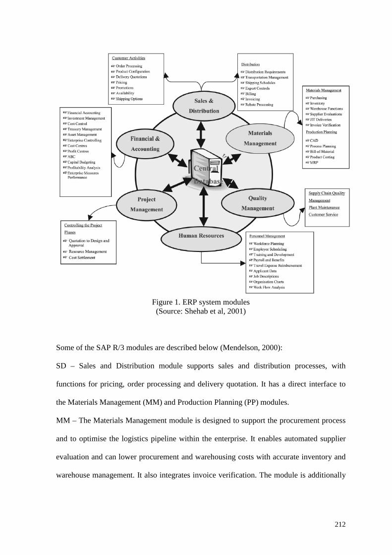
212
Figure 1. ERP system modules (Source: Shehab et al, 2001)
Some of the SAP R/3 modules are described below (Mendelson, 2000):
SD – Sales and Distribution module supports sales and distribution processes, with
functions for pricing, order processing and delivery quotation. It has a direct interface to
the Materials Management (MM) and Production Planning (PP) modules.
MM – The Materials Management module is designed to support the procurement process
and to optimise the logistics pipeline within the enterprise. It enables automated supplier
evaluation and can lower procurement and warehousing costs with accurate inventory and
warehouse management. It also integrates invoice verification. The module is additionally

213
designed to support foreign trade processing, such as customs declarations. Tools for
inventory control and purchasing information help to identify trends and developments.
PP – The Production Planning module supports production planning, manufacturing
processes execution, analysis and production control. This application covers the
production process from the creation of master data to production planning, MRP, and
capacity planning, right down to production control and costing. It supports a variety of
manufacturing processes including repetitive, make-to-order and assemble-to-order
production. Quality management, laboratory information systems and data analysis
functions are also available.
3. ERP Advantages
There are many advantages in the application of the ERP system within a company. Leon
(2008) differentiates between direct and indirect advantages. The direct advantages include
improved efficiency, information integration for better decision making, and faster
response time to customer queries. The indirect benefits include better corporate image,
improved customer goodwill and customer satisfaction. Further, Gargeya and Brady (2005)
provide more detail on the benefits of the implementation of the ERP system in Table 3.
Table 3 Tangible and intangible benefit of ERP system
Tangible benefits Intangible benefits Inventory reduction Personnel reduction Productivity improvements Order management improvements Financial cycle improvements Information technology cost reduction Procurement cost reduction Cash management improvement Revenue/profit increase Transportation/logistics cost reduction Maintenance reductions On-time delivery improvements
Information visibility New/improved processes Customer responsiveness Cost reductions Integration Standardization Flexibility Globalization Supply/demand chain Business performance Dismantling inefficient legacy system

214
Unlike Gargeya and Brady (2005) and Leon (2008), Shang and Seddon (2000) use
different perspective for analysing the benefits of the ERP system. They classified the
benefits into five types:
• Operational benefits. Cost reduction, cycle time reduction, productivity improvement,
quality improvement, and customer services improvement.
• Managerial benefits. Better resource management, better decision making, and
planning and performance improvement.
• Strategic benefits. Supports business growth, supports business alliance, builds
business innovations, builds cost leadership, generates product differentiation, and
builds external linkages.
• It infrastructure benefits. Builds business flexibility, IT costs reduction, and increased
IT infrastructure capability.
• Organisational benefits. Supports business organisational changes; facilitates business
learning, encourages empowerment, and builds common visions.

215
Appendix C: WEEE Directive
According to the Eurostat (2012), the growth of waste electrical and electronic equipment
(WEEE) in the European Union (EU) is at 3-5% and is growing exponentially. As WEEE
puts health and the environment at risk, the EU has been promoting legislation for
collecting and recycling WEEE since February 2003 (WEEE Directive 2002/96/EC). UK
law introduced2006 WEEE Regulations in January 2007. The annual production of WEEE
in the UK is around 2 million tonnes (EA, 2012).
The purpose of this directive is to increase the recycling and/or reuse of WEEE. Moreover,
it also seeks to improve the environmental performance of all operators involved in the life
cycle of electrical and electronic equipment (EEE), e.g. producers, distributors and
consumers, and in particular those operators directly involved in the treatment of waste
electrical and electronic equipment. Towards this aim, the WEEE Directive sets collection,
recycling and recovery targets for all types of EEE goods and can be seen in below table.
Table 1. Minimum rates for separate collection of WEEE (source: Eurostat, 2012)
Date Annual minimum collection rate By 31 December 2015
At least 4 kg / inhabitant of WEEE from private households; OR the same weight as the average amount of WEEE collected in that Member State in the three preceding years; whichever of the two figures that is highest shall continue to apply.
From 2016 to 2018 45% of EEE put on the market, calculated on the basis of: - the total weight of WEEE collected; and - the average weight of EEE put on the market in the three preceding years.
As of 2019 65% of EEE put on the market, calculated on the basis of: - the total weight of WEEE collected; and - the average weight of EEE put on the market in the three preceding years. OR 85% of WEEE generated on the territory of that Member State. As of 2019 (Member States will be able to choose which one of these two equivalent ways to measure the target they wish to report.)
216
The EEE goods covered by the WEEE regulations are those which (EA, 2012):
• are dependent on electric currents or electromagnetic fields in order to work properly,
including equipment for the generation, transfer and measurement of such currents and
fields;
• are designed for use with a voltage rating not exceeding 1,000V for alternating current
and 1,500V for direct current;
• fall into one of the 10 categories in Schedule 1 of the WEEE: Large household
appliances; Small household appliances; IT and Telecommunications equipment;
Consumer equipment; Lighting equipment; Electrical and electronic tools; Toys,
leisure and sports equipment; Medical devices; Monitoring and control instruments;
and Automatic dispensers.
Further, details of EEE under each category can be found at http://www.environment-
agency.gov.uk/business/topics/waste/32120.aspx
The WEEE Regulations place legal obligations on the following types of organisations that
handle EEE (EA, 2012): importers, rebranders and manufacturers; operators of producer
compliance schemes; waste management industry; retailers; business users; householders;
and local authorities.
There are two options for the retailer/distributor to comply with the WEEE regulations in
the UK (DFT, 2012):
• Option A: Offer customers the opportunity to return their WEEE in store, free of
charge when purchasing a similar item or an item for similar use as their old
equipment. If customers wish the retailer/distributor to collect, then a reasonable fee
may be charged. The retailer/distributor is required to record the amount of WEEE
returned.

217
• Option B: Join the Distributor Take Back Scheme (DTS) which is run by an appointed
company. Under this scheme the retailer/distributor does not have to take back any
waste electrical and electronic equipment (WEEE); instead the company will supply
the retailer/distributor with all the information needed in directing customers to their
nearest recycling facility.
Moreover, regardless of business size and quantities of EEE placed on the market,
producers (importers, re-branders or manufacturers) of EEE have responsibilities under
WEEE Regulations and should be registered with an approved producer compliance
scheme (EA, 2012). In addition, for the manufacturer of EEE, extra WEEE rules must be
followed, including labeling products (e.g. use the crossed-out wheelie bin symbol),
marking products (eg. use producer’s identification mark), and producing products that are
easy to repair and recycle (Gov. UK, 2012).
As a major international electronics manufacturer relies on service parts, the case study
organisation made some changes for the purpose of facing this regulation. For example, the
company managers had to rearrange their service parts management. Managers now need
to give more attention to their stock control policy, especially for critical and obsolete
items since the spare/service parts demand pattern is intermittent in nature (this introduces
slow moving items). In addition, managers had to arrange the procedure of reuse,
recycling, and waste collection of their products in order to show their responsibility as
regards the environment.

218
Appendix D: RoHS Directive
Restriction of Hazardous Substances Directive (RoHS) 2002/95/EC is EU legislation
restricting the use of certain hazardous substances in electrical and electronic (EEE)
equipment. The directive has been in force since February 2003 (EC, 2012). This directive
came into force in the UK on 1 July 2006 (NMO, 2012a). Currently, it has been recast and
will be repealed by Directive 2011/65/EU (RoHS 2) with effect from 3 January 2013. The
authorities responsible for enforcing the RoHS Regulations within the UK are the
Department for Business, Innovation and Skills (BIS) and the National Measurement
Office (NMO) (NMO, 2012b).
The objective of RoHS Directive is to prevent all new electrical and electronic equipment
put in the European Economic Area from containing certain levels of hazardous
substances. It restricts the use of lead (Pb), mercury (Hg), cadmium (Cd), hexavalent
chromium (Cr6+), polybrominated biphenyls (PBB) and polybrominated diphenyl ether
(PBDE). The weight of substance at raw homogeneous material must be less than 0.01%
for cadmium and hexavalent chromium and less than 0.1% for lead, PBB, and PBDE. For
mercury, any RoHS compliant component must have 100 ppm or less of mercury and the
mercury must not have been intentionally added to the component. EEE that has to comply
with the RoHS Directive also applies with the WEEE directive, except for medical devices
and monitoring and control equipment (NMO, 2012c).
Under this regulation, EEE’s producers must ensure that their products meet the
requirement of the directive. As a result, producers have to retain technical documentation
showing that their equipment complies with the RoHS Regulations. This documentation
must be retained for inspection for four years from the date the equipment is put on the
market. The producer can refer to the manufacturer, seller, reseller or importer/exporter of
EEE.

219
As the case study organisation can be categorized as a producer of EEE, this regulation
may have a considerable impact on service parts management. Several changes were
implemented in order to face these regulations. For example, the spare parts managers in
all European sites had to scrap parts that are used in new EEE as they may have contained
hazardous substances. Consequently, the implementation of these changes may have an
impact on their supply chain of spare parts.

220
Appendix E: The results of goodness of fit test of Final OUT
replenishment level adjustment distribution across SKUs
A items
Significant level (α) 0.2 0.1 0.05 0.02 0.01 Critical value 0.28072 0.03199 0.03553 0.03971 0.04262
1. Signed size of adjustment
No. Distribution K-S statistic 1 Cauchy 0.05081 2 Error Function 0.21506 3 Gumbel max 0.27602 4 Gumbel min 0.23985 5 Hypersecant 0.19328 6 Laplace 0.16815 7 Logistic 0.20564 8 Normal 0.22109 9 Uniform 0.25375
2. Absolute size of adjustment
No. Distribution K-S statistic 1 Gamma 0.55447 2 Weibull 0.12364 3 Uniform 0.40768 4 Gumbel max 0.42906 5 Normal 0.37456 6 Logistic 0.35892 7 Cauchy 0.25043 8 Gumbel min 0.39951 9 Exponential 0.29863

221
3. Relative signed size of adjustment
No. Distribution K-S statistic 1 Cauchy 0.12128 2 Error Function 0.17219 3 Gumbel max 0.07229 4 Gumbel min 0.15403 5 Hypersecant 0.12301 6 Laplace 0.15139 7 Logistic 0.10961 8 Normal 0.09255 9 Uniform 0.12191
4. Relative absolute size of adjustment
No. Distribution K-S statistic 1 Weibull 0.07066 2 Gamma 0.07483 3 Gumbel max 0.07881 4 Gumbel min 0.19590 5 Logistic 0.12609 6 Normal 0.14199 7 Exponential 0.16516 8 Cauchy 0.13101 9 Uniform 0.17574
B items
Significant level (α) 0.2 0.1 0.05 0.02 0.01 Critical value 0.01973 0.02249 0.02497 0.02791 0.02995
1. Signed size of adjustment
No. Distribution K-S statistic 1 Cauchy 0.03298 2 Error Function 0.26504 3 Gumbel max 0.31353 4 Gumbel min 0.31991 5 Hypersecant 0.23728 6 Laplace 0.21199 7 Logistic 0.24711 8 Normal 0.26301 9 Uniform 0.30013

222
2. Absolute size of adjustment
No. Distribution K-S statistic 1 Gamma 0.30334 2 Weibull 0.17370 3 Uniform 0.37830 4 Gumbel max 0.38433 5 Normal 0.33767 6 Logistic - 7 Cauchy 0.14382 8 Gumbel min 0.35941 9 Exponential 0.17086
3. Relative signed size of adjustment
No. Distribution K-S statistic 1 Cauchy 0.12718 2 Error Function 0.14914 3 Gumbel max 0.09489 4 Gumbel min 0.14876 5 Hypersecant 0.12668 6 Laplace 0.15216 7 Logistic 0.11126 8 Normal 0.13095 9 Uniform 0.18558
4. Relative absolute size of adjustment
No. Distribution K-S statistic 1 Weibull 0.12458 2 Gamma 0.13329 3 Gumbel max 0.21374 4 Gumbel min 0.31545 5 Logistic 0.24153 6 Normal 0.24931 7 Exponential 0.22385 8 Cauchy 0.09897 9 Uniform 0.26519

223
Appendix F: Results of fitting distribution test on Final OUT replenishment level across period
The results of fitting distribution test on Final OUT replenishment level across period for A items
Relative Absolute
Fit Test Sig. LevelFit Test Sig. LevelFit Test Sig. LevelFit Test Sig. LevelFit Test Sig. LevelFit Test Sig. LevelFit Test Sig. LevelFit Test Sig. LevelFit Test Sig. Level
Strong Fit 85.00% 98.75% 31.25% 41.25% 88.75% 95.00% 86.25% 97.50% 52.50% 80.00% 72.50% 85.00% 75.00% 88.75% 76.25% 93.75% 86.25% 97.50%
Fit 12.50% 8.75% 5.00% 10.00% 18.75% 15.00% 13.75% 15.00% 8.75%
No Fit 2.50% 1.25% 60.00% 58.75% 6.25% 5.00% 3.75% 2.50% 28.75% 20.00% 12.50% 15.00% 11.25% 11.25% 8.75% 6.25% 5.00% 2.50%
Size Absolute
Fit Test Sig. LevelFit Test Sig. LevelFit Test Sig. LevelFit Test Sig. LevelFit Test Sig. LevelFit Test Sig. LevelFit Test Sig. LevelFit Test Sig. LevelFit Test Sig. Level
Strong Fit 72.50% 92.50% 42.50% 66.25% 76.25% 97.50% 73.75% 93.75% 35.00% 68.75% 61.25% 83.75% 61.25% 85.00% 63.75% 92.50% 68.75% 90.00%
Fit 12.50% 18.75% 17.50% 17.50% 28.75% 18.75% 21.25% 20.00% 18.75%
No Fit 15.00% 7.50% 38.75% 33.75% 6.25% 2.50% 8.75% 6.25% 36.25% 31.25% 20.00% 16.25% 17.50% 15.00% 16.25% 7.50% 12.50% 10.00%
Relative Sign
Fit Test Sig. LevelFit Test Sig. LevelFit Test Sig. LevelFit Test Sig. LevelFit Test Sig. LevelFit Test Sig. LevelFit Test Sig. LevelFit Test Sig. LevelFit Test Sig. Level
Strong Fit 83.75% 100.00% 17.50% 35.00% 68.75% 86.25% 42.50% 68.75% 53.75% 86.25% 48.75% 76.25% 57.50% 88.75% 58.75% 91.25% 63.75% 93.75%
Fit 13.75% 13.75% 13.75% 23.75% 23.75% 22.50% 20.00% 21.25% 22.50%
No Fit 2.50% 0.00% 68.75% 65.00% 17.50% 13.75% 33.75% 31.25% 22.50% 13.75% 28.75% 23.75% 22.50% 11.25% 20.00% 8.75% 13.75% 6.25%
Size Sign
Fit Test Sig. LevelFit Test Sig. LevelFit Test Sig. LevelFit Test Sig. LevelFit Test Sig. LevelFit Test Sig. LevelFit Test Sig. LevelFit Test Sig. LevelFit Test Sig. Level
Strong Fit 80.00% 97.50% 16.25% 42.50% 58.75% 78.75% 61.25% 82.50% 61.25% 92.50% 55.00% 83.75% 65.00% 96.25% 68.75% 97.50% 66.25% 98.75%
Fit 7.50% 20.00% 23.75% 18.75% 22.50% 20.00% 18.75% 17.50% 25.00%
No Fit 12.50% 2.50% 63.75% 57.50% 17.50% 21.25% 20.00% 17.50% 16.25% 7.50% 25.00% 16.25% 16.25% 3.75% 13.75% 2.50% 8.75% 1.25%
Cauchy Error Gum Max Gum Min Hypersecant Laplace Logistic Normal Uniform
Normal Uniform
Normal Uniform Weibull
Cauchy Error Gum Max Gum Min Hypersecant Laplace Logistic
Normal Uniform Weibull
Cauchy Exponential Gamma Gum Max Gum Min Logistic
Cauchy Exponential Gamma Gum Max Gum Min Logistic

224
The results of fitting distribution test on Final OUT replenishment level across period for B items
Relative Absolute
Fit Test Sig. LevelFit Test Sig. LevelFit Test Sig. LevelFit Test Sig. LevelFit Test Sig. LevelFit Test Sig. LevelFit Test Sig. LevelFit Test Sig. LevelFit Test Sig. Level
Strong Fit 95.00% 97.50% 50.00% 52.50% 92.50% 95.00% 87.50% 87.50% 57.50% 65.00% 87.50% 87.50% 87.50% 85.00% 80.00% 87.50% 92.50% 95.00%
Fit 2.50% 30.00% 5.00% 7.50% 25.00% 2.50% 2.50% 10.00% 5.00%
No Fit 2.50% 2.50% 20.00% 47.50% 2.50% 5.00% 5.00% 12.50% 17.50% 35.00% 10.00% 12.50% 10.00% 15.00% 10.00% 12.50% 2.50% 5.00%
Size Absolute
Fit Test Sig. LevelFit Test Sig. LevelFit Test Sig. LevelFit Test Sig. LevelFit Test Sig. LevelFit Test Sig. LevelFit Test Sig. LevelFit Test Sig. LevelFit Test Sig. Level
Strong Fit 90.00% 92.50% 62.50% 62.50% 97.50% 95.00% 95.00% 95.00% 52.50% 57.50% 72.50% 77.50% 72.50% 82.50% 72.50% 82.50% 95.00% 95.00%
Fit 7.50% 12.50% 0.00% 2.50% 20.00% 20.00% 20.00% 22.50% 2.50%
No Fit 2.50% 7.50% 25.00% 37.50% 2.50% 5.00% 2.50% 5.00% 27.50% 42.50% 7.50% 22.50% 7.50% 17.50% 5.00% 17.50% 2.50% 5.00%
Relative Sign
Fit Test Sig. LevelFit Test Sig. LevelFit Test Sig. LevelFit Test Sig. LevelFit Test Sig. LevelFit Test Sig. LevelFit Test Sig. LevelFit Test Sig. LevelFit Test Sig. Level
Strong Fit 95.00% 100.00% 52.50% 57.50% 85.00% 92.50% 70.00% 77.50% 82.50% 87.50% 72.50% 75.00% 85.00% 90.00% 85.00% 87.50% 85.00% 90.00%
Fit 2.50% 27.50% 10.00% 17.50% 12.50% 17.50% 10.00% 10.00% 10.00%
No Fit 2.50% 0.00% 20.00% 42.50% 5.00% 7.50% 12.50% 22.50% 5.00% 12.50% 10.00% 25.00% 5.00% 10.00% 5.00% 12.50% 5.00% 10.00%
Size Sign
Fit Test Sig. LevelFit Test Sig. LevelFit Test Sig. LevelFit Test Sig. LevelFit Test Sig. LevelFit Test Sig. LevelFit Test Sig. LevelFit Test Sig. LevelFit Test Sig. Level
Strong Fit 85.00% 90.00% 57.50% 60.00% 75.00% 77.50% 85.00% 87.50% 70.00% 77.50% 70.00% 70.00% 80.00% 82.50% 85.00% 90.00% 95.00% 92.50%
Fit 12.50% 20.00% 12.50% 12.50% 27.50% 17.50% 17.50% 12.50% 5.00%
No Fit 2.50% 10.00% 22.50% 40.00% 12.50% 22.50% 2.50% 12.50% 2.50% 22.50% 12.50% 30.00% 2.50% 17.50% 2.50% 10.00% 0.00% 7.50%
Uniform
Cauchy Error Gum Max Gum Min Hypersecant Laplace Logistic Normal Uniform
Uniform Weibull
Cauchy Error Gum Max Gum Min Hypersecant Laplace Logistic Normal
Normal Uniform Weibull
Cauchy Exponential Gamma Gum Max Gum Min Logistic Normal
Cauchy Exponential Gamma Gum Max Gum Min Logistic

225
Appendix G: Explanation of reason categories
I-No reason, D-No reason:
Managers change the OUT level without having any reason. They simply intervene
to the process regardless of whether they possess some important information or
not. No justifications are recorded.
I-Backorder:
Managers make adjustment to increase the OUT level because current stock level is
insufficient to satisfy demand.
I-Low stock, D-Over stock:
Managers adjust to increasing or reducing OUT level by considering current on-
hand inventory.
I-Certain period:
Managers increase the OUT level based on past information in which demand
increased in particular time.
I-Steady demand, D-Steady demand:
Although the demand is steady, sometimes managers make adjustments to
increase/decrease the OUT level. It seems adjustments reflect a desire for a sense of
ownership on the part of the managers.
I-Increasing demand, D-Decreasing demand:
Managers change the OUT level as the demand patterns which tend to increase or
decrease over time.
I-Order spike, D-Order spike:
Managers make adjustment to increase/decrease OUT level based on past
information regarding order spike.
I-Min ROP, D-Min ROP:
Managers increase/decrease OUT level up to minimal OUT level (Min OUT level
is 3 units)
I-Large demand, D-Hardly demand:
The reason for changing the OUT level (increase/decrease) because the demand is
very large or there is no demand on particular material.
I-ROP too low:
Managers adjust to increase OUT level because the current OUT level seems to low
compare with demand on the past.

226
I-Flat average:
Managers decide to increase the OUT level based on the flat average forecasting
information.
I-Replacement part, D-Replacement part:
Managers adjust to increase/decrease OUT level as the material is a replacement
part.
I-Not classified yet, D-Not classified yet:
Managers increase/decrease the OUT level based on a very specific reason where
researcher does not know yet in which category it for.
D-Slow demand:
Managers decided to decrease the OUT level as the item is categorised as the slow
demand.
D-Bulk order:
Decreasing the OUT level because there is bulk order.

227
Appendix H – List of Code
Dim i As Long, t As Long, Positive_Inventory_Position As Single, Investment As Double,
Price As Double, Ave_Positive_Inventory_Position As Double
Dim NegativeStock As Long, Proportion_NegativeStock As Double, BackorderedDemand
As Long, TotalDemand As Long, FillRate As Double
For i = 1 To 1454
'For t = 4 To 27
'Worksheets("stock").Cells(i + 2, t) = Worksheets("stock").Cells(i + 2, t - 1) -
Worksheets("Demand").Cells(i + 2, t) + Worksheets("Order").Cells(i + 2, t - 2)
'If Worksheets("ROP").Cells(i + 2, t) > Worksheets("stock").Cells(i + 2, t) Then
'Worksheets("Order").Cells(i + 2, t) = Worksheets("ROP").Cells(i + 2, t) -
Worksheets("stock").Cells(i + 2, t)
'Else
'Worksheets("Order").Cells(i + 2, t) = 0
'End If
'Next t
For t = 4 To 27
Worksheets("stock").Cells(i + 2, t) = Worksheets("stock").Cells(i + 2, t - 1) -
Worksheets("Demand").Cells(i + 2, t) + Worksheets("Order").Cells(i + 2, t - 2)
If Worksheets("ROP").Cells(i + 2, t) > Worksheets("stock").Cells(i + 2, t) Then
Worksheets("Order").Cells(i + 2, t) = Worksheets("ROP").Cells(i + 2, t) -
Worksheets("ROP").Cells(i + 2, t - 1) + Worksheets("Demand").Cells(i + 2, t)
Else
Worksheets("Order").Cells(i + 2, t) = 0
End If
Next t
Inventory_Position = 0
For t = 4 To 27
Inventory_Position = Inventory_Position + Worksheets("stock").Cells(i + 2, t)
Next t
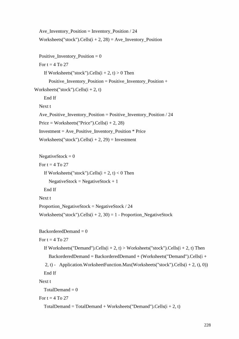
228
Ave_Inventory_Position = Inventory_Position / 24
Worksheets("stock").Cells(i + 2, 28) = Ave_Inventory_Position
Positive_Inventory_Position = 0
For t = 4 To 27
If Worksheets("stock").Cells(i + 2, t) > 0 Then
Positive_Inventory_Position = Positive_Inventory_Position +
Worksheets("stock").Cells(i + 2, t)
End If
Next t
Ave_Positive_Inventory_Position = Positive_Inventory_Position / 24
Price = Worksheets("Price").Cells(i + 2, 28)
Investment = Ave_Positive_Inventory_Position * Price
Worksheets("stock").Cells(i + 2, 29) = Investment
NegativeStock = 0
For t = 4 To 27
If Worksheets("stock").Cells(i + 2, t) < 0 Then
NegativeStock = NegativeStock + 1
End If
Next t
Proportion_NegativeStock = NegativeStock / 24
Worksheets("stock").Cells(i + 2, 30) = 1 - Proportion_NegativeStock
BackorderedDemand = 0
For t = 4 To 27
If Worksheets("Demand").Cells(i + 2, t) > Worksheets("stock").Cells(i + 2, t) Then
BackorderedDemand = BackorderedDemand + (Worksheets("Demand").Cells(i +
2, t) - Application.WorksheetFunction.Max(Worksheets("stock").Cells(i + 2, t), 0))
End If
Next t
TotalDemand = 0
For t = 4 To 27
TotalDemand = TotalDemand + Worksheets("Demand").Cells(i + 2, t)

229
Next t
If TotalDemand > 0 Then
FillRate = (TotalDemand - BackorderedDemand) / TotalDemand
Else
FillRate = 0
End If
Worksheets("stock").Cells(i + 2, 31) = FillRate
Next i
End Sub