Infrastructure Effectiveness as a Determinant of Economic Growth:How Well You Use it May Be More Important than How Much You Have

Charles R. Hulten University of Maryland

and NBER

December 1996Revised December 2005

I would like to thank the many people who gave on earlier draft (NBER WorkingPaper 5847), and Ioannis Kessides for his comments on this draft. Remainingerrors, etc., are my own.

1 Development economists have long recognized that social overheadcapital is a necessary input in the structure of production (e.g.,Hirschman (1958)). Infrastructure was incorporated into formal growththeory by Arrow and Kurz (1970) and Weitzman (1970). Empirical studiesof the importance of infrastructure as a source of growth gainedprominence with the papers of Aschauer (1989a,1989b), which werefollowed by a large body of econometric research. The more generalcapital formation sources-of-growth literatures are surveyed in Hulten(1990, 2001).

1

I. Introduction

Most contemporary explanations of economic growth assign a prominent

role to capital formation. This includes the huge literate of the sources of

economic growth in the tradition of Solow (1957) and Jorgenson and Griliches

(1967), but it also includes the smaller literature on social overhead capital

and public infrastructure.1 However, this literature has focused primarily on

investment in new capital goods, and comparatively little attention has been

given to the effective use of capital stocks once they are in place. This is

a potentially important omission, since it is the flow of services from the

stock, not the stock itself, that influences output. If this flow is

diminished by the inefficient operation of the stock, or by its poor

condition, additional capital formation may be of little help in stimulating

economic growth.

The relative neglect of the effectiveness dimension of infrastructure

capital is due largely to the scarcity of appropriate data. Fortunately,

there is one major exception to this problem: the 1994 issue of the World

Bank’s World Development Report (WDR) is devoted to role played by

infrastructure investment in the process of economic development and contains

estimates of the effectiveness of various infrastructure systems in a broad

cross-section of developing counties for a single year. This study revealss a

significant problem with the reliability and condition of the systems studied.

One finding suggests that $12 billion in timely road maintenance in Africa

over the preceding decade would have avoided the need for $45 billion in

reconstruction and rehabilitation. Moreover, "inadequate maintenance means

that power systems in developing countries have only 60 percent of their

2

generating capacity available at a given time, whereas best practice would

achieve levels of 80 percent ... [and] water supply systems deliver an average

of 70 percent of their output to users, compared with best-practice delivery

rates of 85 percent (page 4)." The WDR goes on to note that these

deficiencies often arise from inadequate management of the existing

infrastructure assets, as distinct from inadequate levels of new construction.

This is seconded by the remark by Easterly and Levine (1996) that, while Chad

may have 15,000 telephones, 91 percent of all telephone calls are

unsuccessful.

The existence of an infrastructure effectiveness problem is therefore a

well-documented phenomenon, and the corresponding penalty that it imposes on

output was investigated by Lee and Anas (1992), who found that an unreliable

electrical supply limited the use of certain types of machinery, putting

companies at a competitive cost disadvantage. However, the overall penalty on

macroeconomic economic growth arising from was not estimated in the WDR (or

elsewhere), so it is hard to say just how quantitatively important the

infrastructure effectiveness problem as a barrier to economic development.

Assessing the magnitude of this growth penalty at the macroeconomic

level of growth is the main goal this paper. A summary effectiveness

indicator is derived from the separate WDR indexes and the result is then

embedded in a model of economic growth in order to assess the importance of

the factor as a co-determinant of long-run output per capita. The model

developed by Mankiw, Romer, and Weil (1992) (hereafter “MRW”) is used for this

purpose. The resulting estimates for a sample of 46 low and middle income

countries, covering the period 1970 and 1990, suggest that infrastructure

effectiveness is an important factor in explaining differences in rates of

real GDP growth during this period, even after controlling for various

dimensions of political instability. This kind of control is needed in order

to allow for possibility that the infrastructure effectiveness index is acting

as a surrogate for a more general productive inefficiency that extends beyond

infrastructure. With these controls, the estimate of the direct

infrastructure penalty implies that a one-percent decrease in the

3

infrastructure effectiveness index reduces the output by 0.51 percent. When

the dynamic effects of this penalty are taken into account, the long-run

penalty is estimated to be even larger, 0.79 percent. Cross-national

differences in growth are also large: the 13 countries with the least

efficient infrastructure have an average effectiveness index of 37 (out of

100) and an average annual growth rate of -0.70%; the 14 above average

countries have an index value of 78 and an average annual growth rate of

2.68%. Viewed yet another way, the absolute level of productive efficiency is

30 percent lower at each point in time (relative to what might have been

achieved) because infrastructure is used ineffectively. That is, the average

country in the sample could increase output by 30 percent by using its

existing capital and labor resources more effectively.

II. A Model of Infrastructure Effectiveness and Economic Growth

1. Economic efficiency is, at one level, a matter of the technology and

organization of production, but at deeper level, it is a reflection of

underlying societal institutions and culture. It is not easy to bring the two

together in an analysis of growth. The literature on the estimation of

production functions, as well as the literature on the measurement of total

factor productivity, simply treats economy efficiency as a technical parameter

to be estimated, usually as a residual, with no attempt to get at its deeper

determinants. Observed changes in productive efficiency over time are

interpreted as ‘technical change’ in the productivity literature (cite Hulten

(2001)). When the focus is on cross-country comparisons of economic growth,

as in this paper, the usual approach is to treat measured differences in

factor efficiency as an indicator of the gap between the best practice

technology and the actual level of technology in each country (cite Young, TFP

catch up). In this context, measuring the contribution of infrastructure

inefficiency to this gap is one way to get at the size of the associated

growth penalty.

The literature of growth and development, on the other hand, does

2 In the special case in which all factor input are equally influencedby technical change, the production function has the well-known Hicks’-neutral form Yi,t = Ai,t F(Li,t,Ki,t,Gi,t). The model developed below makesuse of this specification in combination with a separate factor-augmentation parameter for infrastructure.

4

(1)

introduce institutional and cultural variables into the analysis, but

typically without a specific link to the structure of production. The issue

of infrastructure effectiveness lies somewhere between these two literatures.

From the standpoint of production theory, all inputs to production are subject

to variations in the efficiency with which they are used to production output.

In the model of factor-augmenting technical change, each input is multiplied

by a scalar index that represents the efficiency with which the input is used.

Infrastructure inefficiency has a natural interpretation in this model as the

factor-augmentation parameter associated with the stock of infrastructure

capital. The resulting production function in this case is

Yi,t denotes real output in country i in year t, Li,t is labor input, and Ki,t

and Gi,t are the stocks of private and public capital, respectively. The

corresponding factor-augmentation indexes are [Ni,t,Ri,t,Ti,t], with Ti,t

representing infrastructure efficiency index.

Technical change over time occurs, in this specification, when the

indexes increase over time because of improvements in the organization of

production and because technological improvements allow the inputs to be used

more efficiently. Cross-sectional differences in the indexes at any point in

time are interpreted as the penalty gap between potential and actual

productive efficiency in country i.2

The factor-augmentation index, Ti,t, can be given additional structure by

making it an explicit function of the index of infrastructure effectiveness,

2i,t. We will assume, for simplicity, that the function has the constant

elasticity form

3 In this formulation, the infrastructure effectiveness index, 2i,t, istreated as a scalar index that applies to the stock of infrastructure asa whole. In reality, infrastructure facilities tend to be congestiblepublic goods that are organized into capital-intensive networks (e.g.,roads and bridges, railroads, air and water transport, water and sewersystems, electricity generation and distribution networks,telecommunications facilities). Each segment of the network couldplausibly be regarded as a separate investment, with it’s own efficiencyindex. The index 2i,t used in this paper is an aggregate indicator ofthe system as a whole, a sort of weighted average across the entiresystem. By implication, some parts of network which may actually workefficiently, with the further implication that the same value of 2i,t intwo countries may imply have different policy implications.

5

(2)

This formulation links the effectiveness of a country’s infrastructure

directly to its real GDP, by inserting (2) into the production function (1)

and observing that the elasticity of output with respect to the measured index

2i,t is simply the parameter D times the GDP share of infrastructure (or D(,

where the share is denoted by (). This implies that each one-percent decline

in infrastructure efficiency reduces real GDP by D( percent. This is the

direct penalty that the inefficient use of infrastructure exacts on economic

growth.3

2. The factor-augmentation parameters are usually taken as determined outside

the estimation model. Even the step taken in the formulation of (2) is

somewhat unusual, though it does have some precedent (e.g., in the literature

on the contribution of R&D to economic growth). However, the efficiency with

which infrastructure and other inputs are used may itself be a reflection of

deeper causal factors, like bureaucratic red tape, over-regulation of firms,

inflexible labor markets, corruption, weak enforcement of property rights, and

civil unrest. If these latent “X” factors change only gradually over time,

they can safely be treated as exogenous parameters in the in the production

function, to be measured but not explained. In cross-sectional studies,

however, it is precisely these factors that may contribute the most to

national differences in economic growth. In terms of the factor-augmentation

model, the index 2i,t might itself depend on a set of these “X” factors. In

4 In the simplest version of the Solow growth model, output per workerconverges to a steady-state growth path along with the growth rates ofoutput and capital equal the growth rate of the labor force. Convergence occurs according to the following mechanism. A constantfraction of the output, s, is set aside in each year for investment,which increases the stock of capital. If the increase in capital isgreater than the growth in the labor force, capital per worker expands,increase output per worker in the next year. The fraction s of this

6

this case, the index has the form 2(Xi,t), thus making Ti,t a function of these

factors as well. Moreover, the latent “X” characteristics so might also

influence the augmentation parameters for labor and private capital, Ni,t and

Ri,t. In this situation, the elasticity of output with respect to an index of

the X-efficiency variables might be considerably larger than D(, and any

attempt to force the whole effect onto the infrastructure variable might over-

state the role of infrastructure effectiveness.

3. The primary goal of this paper is to isolate and estimate the

infrastructure inefficiency penalty, D(, and its variants and correlates. The

straightforward way to proceed, in view of (1) and (2), is to specify a

specific functional form for the production function and to estimate the

magnitudes D and (. However, there are two problems with the direct

estimation of the production function. First, there is the practical issue

that estimates of the stocks of public and private capital are of problematic

reliability for some developing countries, and they may not exist at all for

some countries. But, second, even if when reliable data data are available,

direct estimation the production function is subject to the problem that the

stocks of capital are jointly determined with output. More capital leads to

more output, and more output leads to more investment and thus more capital,

creating the potential for the simultaneous-equations bias that has plagued

many econometric studies of infrastructure’s affect on output (e.g., Aschauer

(1989a,1989b))

Both of these problems care ameliorated in the approach developed in

Mankiw, Romer, and Weil (1992). This model is based on the Solow (1956) model

of economic growth, in which the rate of saving and not the stock of capital

is the explanatory variable.4 The capital stocks entering the production

larger output is set aside for capital formation, and if the increase incapital is again greater than the growth in the labor force, capital perworker expands, increasing output per worker, and so one. Because ofdiminishing marginal return to capital, each successive increase inoutput per worker is smaller, and the process come to an end when theincrease in capital just equals the growth in the labor force. At thispoint, the steady-sate balanced growth path is attained.

7

function are endogenously determined by accumulation equations for each type

of capital, and by an investment equation in which investment is a constant

fraction of output. This fraction, the rate of investment in each type of

capital is assumed to be exogenously determined (sk,sh,sg), as are the growth

rates of labor, n, labor-augmenting technical change (the rate of change of

Ni,t above), 8, and to depreciation rate of capital, *. The Solow growth model

is thus a system of equations in which the production function is but one

element. MRW solve this system of equations for its reduced form, expressing

the growth rates of output and capital in terms of the exogenous rates of

investment, depreciation, technical change, and labor growth. Since the flow

on investment, and thus the investment rate, is more readily measured than the

corresponding stock of capital, this reduced-form approach is more easily

implemented than direct estimation of the parameters of the production

function. Moreover, because it is more plausible to assume that the rate of

investment is independent of the level of output than to believe that the

stocks are exogenously determined, the problem of simultaneous equations bias

is addressed.

MRW proceed by assuming that the production function has the Cobb-

Douglas form, with constant returns to scale. In this paper, we expand the

MRW specification to includes infrastructure capital and effectiveness

(although MRW actually use a combined concept of physical capital, G+K, in

their study), as well as the X-efficiency variables, and retain the MRW human

capital variable, Hi,t. We will also work with a special case of the general

factor-augmentation model (1), in which the latent X-efficiency variables are

embodied in a general Hicksian efficiency term that shifted the production

function as per footnote X, and in which the infrastructure-efficiency

variable augments the public infrastructure variable as in equation (2).

5Labor is expressed here in efficiency units, e8tLi,t, where 8is the rate of labor-augmenting technical change. Outputper unit of (efficient) labor is then yi,t = Yi,t/e8tLi,t, etc.

8

(3)

Expressed in an “intensive” format, in which the endogenous variables are

divided by labor input, the resulting production function has the form

where (k,h,g) are the per worker magnitudes of private fixed capital, human

capital, and public capital respectively.5 The parameter (",$,() are the

output elasticities with respect to the capital stocks, (k,h,g). Operating

through the shift term A(Xi,t), the latent X-efficiency variables augment each

input equally, implying that “bad” institutions shift a country’s aggregate

production function downward relative to the maximal “best-practice” frontier.

The infrastructure efficiency index also shifts the production function (3)

downward when infrastructure is used inefficiently, but since it is “attached”

to the infrastructure stock variable, the elasticity of output with respect

2i,t is the constant D(.

The Cobb-Douglas production function is solved with the accumulation

equations for each type of capital, and the corresponding investment

equations. A steady state growth path (y*,k*,h*,g*) is shown by MRW to be a

function of the constant investment rates (sk,sh,sg), and the rate at which the

effective work force expands, n+8, plus the constant replacement rate of

capital, *. The sum n+8+* is rate at which capital stocks must grow in order

to keep the capital-labor ratio constant. MRW show that the multiplicative

form of the Cobb-Douglas production function carries over to the reduced form

equations, as do the Cobb-Douglas parameters. The reduced form equations for

steady output per worker, and for each of the types of capital per worker, is

given by:

9

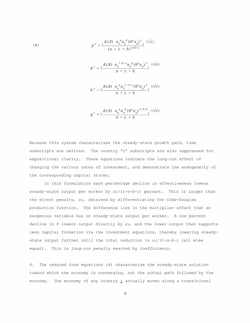
(4)

Because this system characterizes the steady-state growth path, time

subscripts are omitted. The country “i” subscripts are also suppressed for

expositional clarity. These equations indicate the long-run effect of

changing the various rates of investment, and demonstrate the endogeneity of

the corresponding capital stocks.

In this formulation each percentage decline in effectiveness lowers

steady-state output per worker by D(/(1-"-$-() percent. This is larger than

the direct penalty, D(, obtained by differentiating the Cobb-Douglas

production function. The difference lies in the multiplier effect that an

exogenous variable has on steady-state output per worker. A one percent

decline in 2 lowers output directly by D(, and the lower output then supports

less capital formation via the investment equations, thereby lowering steady-

state output further until the total reduction is D(/(1-"-$-( (all else

equal). This is long-run penalty exacted by inefficiency.

4. The reduced form equations (4) characterize the steady-state solution

toward which the economy is converging, not the actual path followed by the

economy. The economy of any country i actually moves along a transitional

10

(5)

path from the initial level of output per worker to the steady state path,

which, following MRW, can be defined by the following expression:

where yi,0 is the level of output per worker in the initial year, yi* the

steady state value toward which the economy is moving, and : the parameter

determining the rate of convergence. This is a partial adjustment model with

an endogenous “target,” yi*, and a rate of adjustment determined by the

parameters equal of the Solow model, : = (n+8+*)(1-"-$-().

The transitional dynamics implied by (5) can be operationalized by

combining this expression with the natural logarithm of first equation of (4).

The resulting equation does not involve the unobserved steady-state, yi*, but

is instead a relation between observable variables that can, in principle, be

estimated. Letting yi,70 denote real GDP per unit of labor in country i in

1970, and yi,90 the 1990 value of this variable, the left-hand side of equation

(5) becomes

(6) ln[yi,90/yi,70] = b0 + 3i biXi + bk ln[ski(ni+8+*)] + bh ln(sh

i/(ni+8+*)]

+ bg ln[sgi/(ni+8+*)] + b2 ln( ) + bc ln(yi,70)) + ,i .

This is the basic regression equation of this paper. Because the regressions

are applied to a cross-section of countries, the time subscripts are largely

absent, but the countries subscripts are included.

The regression parameters (bk,bh,bg) can be interpreted as the

elasticities of growth with respect to the investments rates (ski,sh

i,sgi), b2

as the growth elasticity of infrastructure effectiveness, and bc as the

elasticity of "catch-up." These growth rate elasticities are not the same as

the output elasticities, (",$,(), because of the steady-steady multiplier

effect described above for the infrastructure-effectiveness penalty. They

are, however, related by the formulae: " = bk/(bk+bh+bg-bc), $ = bh/(bk+bh+bg-

bc), and ( = bg/(bk+bh+bg-bc). The level of Hicksian efficiency, Ai, is derived

11

from the constant term and the effects of the latent institutional variables,

by taking the exponent of b0 + 3i biXi, evaluated at the means of the “X”

variables. The rate of convergence, :, is derived from bc. Estimation of the

parameters (bk,bh,bg,bc) thus gives estimates of the output elasticities,

(",$,(), the level of productive efficiency, and the rate of convergence.

III. Data

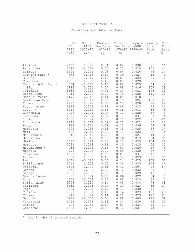
1. The data used in this study are derived from four main sources: the

Easterly-Rebelo (1993) data base, the World Bank's World Development

Indicators, and the 1994 World Development Report, the Summers and Heston

(1991) Penn World Tables. The analysis is restricted to low and middle income

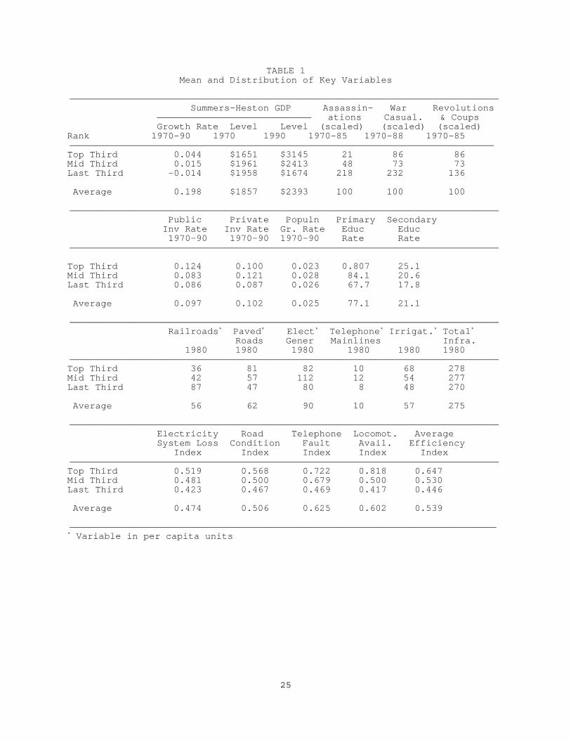
countries, and spans the years 1970 to 1990. A summary list of the variables

is shown in Table 1, along with the data sorted by income-growth rate

terciles. A list of countries in the sample is given in Appendix Table A.

The main income concept used in this paper is based on Summers-Heston

real GDP per capita adjusted for purchasing-power parity, although unadjusted

World Bank estimates of real GDP per capita were also used as a robustness

check. These data are summarized in the top panel of Table 1. The dependent

variable in all regressions is the growth rate of real GDP per capita between

1970 and 1990. The basic right-hand side variables of the regression equation

(6) are the investment rates of public capital/infrastructure, private

capital, and human capital. Various alternatives are used for the public

capital/infrastructure variable, but only one private investment rate is used.

Since no purchasing-power parity adjustment for public or private capital

flows is available in the data bases, all investment rates are expressed as a

fraction of unadjusted GDP, averaged over the period 1970 to 1990. Human

capital was proxied by primary and secondary education enrollment rates, but

expenditures on health and education as a fraction of GDP we also used in some

varaints of the analysis. The investment rates are deflated by the average

rate of population growth between 1970 and 1990, to which is added .05

(following MRW) to allow for the average rate of capital depreciation and

12

labor-augmenting technical change.

The Easterly and Rebelo investment rates are shown in the second panel

of Table 1. The measure of gross public investment is broadly encompassing,

and includes investment by public firms that are similar in function to those

in the private sector. It should be noted that the rate of public investment

differs greatly from the rate of infrastructure investment, which is only 3.0

percent in the 24 countries for which this variable is available. Easterly

and Rebelo indicate that their estimate of infrastructure investment may be

biased downward because it excludes the infrastructure investments of

publicly-owned and private firms.

Another variant of the analysis examined infrastructure stocks rather

than flows. The 1994 World Development Report presents information on the

stock per capita of paved roads, telephone mainlines, electricity generation

capacity, irrigation, and railroads. These data are largely physical

indicators of the total stock, not perpetual inventory estimates. They are

shown in the third panel of Table 1, expressed in 1980 dollars. There is

apparently little difference among the three groups in the total amount of

infrastructure capital, though the composition does change across groups. The

most rapidly growing countries placed more emphasis on road transport than on

rail, and had a larger stock of irrigation capital.

2. Measures of the effectiveness of the various infrastructure systems are

shown in the bottom panel of Table 1. One indicator was selected for each of

the four main systems. These measures are taken as being representative of

the efficiency of the various systems. The construction of an aggregate

effectiveness index is further complicated by the fact that each of the

individual indicators is measured in its own units -- e.g., mainline faults

per 100 telephone calls, electricity generation losses as a percent of total

system output, the percentage of paved roads in good condition, diesel

locomotive availability as percent of the total -- and there is no natural

way of adding up the indicators in this form to arrive at a total. The 1994

WDR did not offer an aggregate measure of performance.

13

Given these difficulties, a simple two-stage procedure is used to

aggregate the individual performance indicators. First, each indicator was

sorted into quartiles, and the top quartile assigned a value of 1.00, the

second, 0.75, the next 0.50, and the bottom assigned a value of 0.25. This

produced a quartile ranking for each of the four systems for each country in

the sample, 2ij. An aggregate indicator for each country, 2i, was computed by

simple averaging of the 2ij. For some countries, the 2ij quartile values were

available for all four systems, but for many countries, the average is taken

over only two or three indicators (countries with only one value were dropped

from the analysis). This averaging procedure retains as many countries as

possible in the sample while making use of data for the different

infrastructure systems. The resulting aggregate index provides a country

ranking according to qualitative performance in those infrastructure functions

for which data are available.

3. The institutional variables used to control for latent sources of economic

inefficiency are derived from two sources. Easterly and Rebelo provide three

such variables in the larger data set used in this paper. They include, for

each country: assassinations per million, 1970-85; revolutions and coups,

1970-85; and, war casualties per capita, 1970-88. These are the “X”

variables used in the estimation of the regression model (6). They are

background variables that can be expected to affect the ability of an economy

to function efficiently. Political instability may affect the production of

output in many ways, including the effectiveness with which infrastructure is

used.

The broad effects on output growth are examined in the following

section, while Table 2 explores the infrastructure dimension. The first

column of this table reports the parameter estimates from the regression of

the log of the infrastructure efficiency index, 2i, on the levels of the three

political stability variables. All the slope coefficients all have the

expected negative sign, although only war casualties per capita is

statistically significant. The R-squared is 0.277, showing the these

14

variables have some explanatory power, but also that there is a great deal of

independent variation in the index 2i. The exponent of the constant term is

an estimate of 2i, when the “X” variables are at the optimal level of zero,

but the resulting value of 0.56 is well below the maximal value of 1.0 (again

suggesting that the institutional variables fall short of explaining the index

2i). Indeed, the fitted “X” terms, 3i biXi, evaluated at the sample means

imply a penalty of only eight percent relative to the maximal value of the

constant term. It is worth noting that the institutional variables are

positively (and significantly) related to the rates of investment in public

and private capital, though the relation is not strong. However, this is no

relation between the institutional variables and the rates of investment in

human capital.

The importance of political instability as a background variable

suggests that is might be useful to extend the analysis to include variables

reflecting economic-cultural institutions as well. The paper by Mauro (1995)

on corruption and growth develops another set of indicators that yield

insights into other dimensions of this penalty: corruption, red tape, and an

efficiency of the judiciary. These are drawn from the measures produced by

Business International. Mauro also develops an index of political

instability from the BI measures and develops a separate index of

ethnolinguistic fractionaliztion. He finds that these variable have a

significant effect on the growth rate of per capita GDP growth in the sample

of countries and time period studied. They can also be incorporated into the

model developed in this paper, but only for a reduced set of 26 countries.

The second column of Table 2 shows the link between the original three

Easterly-Rebelo institutional variables and the index of infrastructure

effectiveness for the 26 country sample. The R-squared is higher than with

the 46 country sample, and now both assassinations and war casualties have

significant coefficients although revolutions has a positive sign. The next

column shows the effect on the effectiveness variable of the core Mauro

variables. The R-squared for this regression is similar to the fit in column

(2). However, only the political stability variable is statistically

15

significant at conventional levels. The last column of the table combines

both sets of variables and achieves an R-squared of 0.613. Unfortunately, the

economic-cultural variables are not statistically significant, again, and the

estimated coefficients of red tape and efficient judiciary both have positive

signs. Although the degrees of freedom are small, the contribution of these

variables is nevertheless disappointing.

IV. Basic Regresson Results

1. A simple plot the growth tare of GDP per capita against the infrastructure

effectiveness variable is shown in Figure 1. This diagram visually indicates

a strong link between the two variables absent any other factors. The implied

OLS regression is ln[yi,90/yi,70] = 0.868 + 1.036 ln(Ni), with an R-squared of

0.504 and a standard error on the infrastructure elasticity of 0.155. This

establishes infrastructure effectiveness as an important correlate of economic

growth. The size of the elasticity, 1.036, also implies a very large (one-to-

one) penalty to the poor use of infrastructure stock, other things equal.

Table 3 presents the results of implementing the full model of equation

(6), based on the 46 country sample. The regressions include the Easterly-

Rebelo institutional variables, but the estimates for these variables are

omitted from the tables to save space and because impact is minimal (their

effects are included estimates of the other variables). The top panel of

Table 3 reports the ordinary least squares estimates of the parameters of the

regression equation (6), along with the associated t-statistics. The implied

elasticities (",$,() are computed from these estimates, and are shown in the

lower panel.

The first column shows the parameter estimates and implied elasticities

without the effectiveness variable, 2. The estimates of the output

elasticities of capital are statistically significant, and their combined

value is similar to the MRW estimate of 0.44 for the combined capital

coefficient (MRW Table VI, 75 country sample). The R-squared statistic is

0.56, slightly greater that the one obtained from the regression of the income

16

per capita variable on 2. The estimated coefficient of the initial (1970) GDP

per capita is statistically significant, implying a rate of convergence of

0.024, which is close to the theoretical value (n+8+*)(1-"-$-() = 0.020. It

is also close to the MRW estimate of 0.0186.

The second column of Table 3 adds 2 to the list of Solow-MRW variables,

and is a full implementation of the regression equation (6). The

infrastructure effectiveness variable enters in strongly significant way, with

a long-run elasticity of 0.794, and the R-squared increases to 0.71. This

result implies a very large long-run penalty: a ten percent reduction in the

efficiency with which infrastructure is used reduces the log-change in income

per capita by 7.94 percent, when the feedback effects of reduced capital

formation are counted. When they are not, the penalty in 0.51. This is the

equivalent to a downward shift in the production function (3) by this factor

for each level of income per capita.

The addition of 2 also reduces the public capital variable to

statistical insignificance, and lowers the significance of private capital and

primary education, while promoting that of secondary education. This

reflects, in part, the correlation between the independent variables

(sk,sh1,sh2,sg): the corresponding partial correlation between these variables

and 2 are 0.42, 0.24, 0.22, and 0.32, respectively. The partial correlation

between sg and 2 may reflect, in part, a virtuous growth environment in which

the decision to invest in public capital and the efficient operation of that

capital are part of the same phenomenon, this could also extend to investment

in private capital and education. Finally, the rate of convergence is, again,

reasonably close to the theoretical value (0.029).

The reduction in the importance of the public capital stock, sg, is

particular notable in light on debate over the role of public investment as a

stimulus to economic growth and development. It suggests that how

infrastructure is used is at least as important as how much there is. It is

worth noting again, in this regard, that public infrastructure systems are

typically networks of individual investments. Adding links to a system that

is not efficiently used may not have much effect on output if the links are

17

themself not efficiently placed (e.g., to relieve congestion), or may not have

much effect at all if the condition or operation of the system as a whole is

poor. Conversely, improvements in system efficiency may have a large effect

of output even if there is little or no new investment in capacity.

The output elasticity of 1 is, in principle, equal to D(. The estimated

output elasticity of the public capital coefficient, (, is 0.069, implying a

value for D equal to 7.78. This seems too large for an exponential term

(recall equation (2)), an it may reflect that the infrastructure variable

acts, in part, as a proxy for the overall degree of economic efficiency of the

economic system, despite having controls for the Easterly-Rebelo institutional

variables. In fact, the Easterly-Rebelo variables do not contribute much to

the explanation of economic growth. None of the variables are statistically

significant and, as column (3) of the table indicates, the effects of omitting

these variables from the analysis are minimal.

The regressions of Table 3 were redone with the Mauro institutional

variables for the 26 countries for which they overlapped with the larger

sample, with the hope that a richer set of institutional variables would serve

as a better control for the assessing the effect of the infrastructure index.

The results were disappointing, in that lagged income per capita was the only

variable that was statistically significant in any of the regression involving

institutional variables. When the regression corresponding to the last column

of Table 3 was performed, that is, without any institutional variables, the

estimated direct effectiveness elasticity, D(, was found to be 0.331 (compared

to 0.496 in Table 3), and the infrastructure stock parameter, (, was 0.158

(compared to 0.046 in Table 3). The fit was also better, with an R-squared of

0.767 versus 0.692 in the larger sample. Thus, the countries in the smaller

Mauro sample were characterized by a stronger infrastructure stock effect and

somewhat weaker efficiency effect.

As with Table 3, adding the Easterly-Rebelo institutional variables had

a minimal effect in the smaller sample. The estimated direct effectiveness

elasticity, D(, fell from 0.331 to 0.286 and the infrastructure stock

parameter, (, rose from 0.158 to 0.160. Neither variables were statistically

18

significant. When the Mauro institutional variables were added, the estimated

direct effectiveness elasticity fell again, this time from 0.286 to 0.266 and

the infrastructure stock parameter from 0.160 to 0.197. Given the large

standard errors on these estimates, the addition of the two sets of

institutional variables did not produce estimates that were statistically

significant from the case in which there was no control for these variables.

This may reflect the rather low degree of freedom available given the

smallness of the sample and the large number of explanatory variables.

2. A number of alternative definitions of the key variables were explored in

order to check the robustness of the estimates in Table 3, and several deserve

special mention. First, estimates were obtained using the World Bank

unadjusted income concept in place of the Summers-Heston PPP-adjusted

estimates. Second, the use of primary and secondary enrollments as proxies

for the rate of investment in human capital was tested by using expenditures

on health and education as a fraction of GDP to estimate the human capital

elasticities. Neither alternative yields results that are significantly at

odds with those of Table 3.

Third, the use of ordinary least squares with a lagged endogenous

variable (ln y(70)) may introduce a bias into the estimates. To control for

this problem, instrumental variables were used to obtain a fitted value for

ln(y(70)); these variables included the infant mortality rate in 1970, the

primary enrollment rate in 1960, and energy consumption per capita in 1970.

The results indicate that the instrumental variables had a negligible effect

on the parameters of interest. Other sets of instruments produced a similar

result.

Fourth, Easterly-Rebelo estimates of investment in infrastructure, as

opposed to investment in public capital, are available for a small number of

countries. The latter averages approximately nine percent of GDP, while the

rate of public infrastructure investment averages only about 3.0 percent. A

shift from a broad to a narrow definition of infrastructure alters the results

considerably, with a large decline in the elasticity of ln sg.

19

Finally, the scatter of points in Figure 1 suggests that the link

between the output growth and infrastructure effectiveness is robust to adding

or deleting countries from sample (a known problem with this type of model).

However, this was checked by subtracting Zambia from the sample. This

increased the estimated public capital coefficient and reduced the

infrastructure effectiveness estimate by a noticeable amount, but not by

enough to alter the conclusions based on the main results. The procedure

adopted in this paper is to present estimates for the maximum number of

countries for which data are available, since there are no a priori reason to

exclude any observation from the sample, but sample composition effects are

potentially important and the results should be interpreted with this in mind.

V. Results II: Stock Measures of Infrastructure

The preceding analysis is based on the assumption that it is the rate of

investment that is exogenously determined, not the capital stock. However, if

the stock of infrastructure capital is the policy variable that the government

seeks to control, the reduced form system (4) has a different form. The Solow

model can be solved with the infrastructure stock as an exogenous variable

instead of the investment rate, in which case the first equation of the

reduced form can be expressed in terms of the stock of infrastructure, g,

rather than the investment rate sg:

(7)

The rest of the steady-state model (4) is modified accordingly. This

modification yields a variant of the basic estimating equation (6) in which

the infrastructure stock replaces the investment rate.

This model was applied to the 1980 values of five types of

infrastructure stock: telephone systems (proxied by telephone mainlines per

capita), road networks (measured as kilometers of paved roads per capita),

20

electric power systems (proxied by electric generating capacity per capita),

railroads (kilometers per capita), and irrigated land area (thousands of

hectares). These stock measure are essentially indicators of physical

capacity, unadjusted for quality or effectiveness difference. The expectation

is thus that the addition of an effectiveness indicator to the analysis will

have a larger impact than in Table 3.

The resulting estimates are shown in Table 4, which is similar to Table

3, except that the aggregate infrastructure stock replaces public investment

as the measure of ln sg. To bridge the gap between the two measures, Column

(1) presents estimates based on the Table 3 measure of public investment and

is comparable to column (1) of that table, except that the analysis is now

limited to the 42 countries for which complete infrastructure stock data is

available (rather than 46). Nevertheless, the omission of four countries in

passing from one to the next has only a small effect on the estimated

parameter elasticities (another robustness check). However, with Table 3, a

large effect is recorded in jumping from the public investment variable of

Column (1) to the aggregate infrastructure stock of column (2). The estimate

of bg falls by a factor of ten, and the t-statistic falls from 2.706 to 0.254.

The importance of effectiveness-adjusted infrastructure as an explanator of

cross-national growth thus disappears.

Some of the explanatory power is restored in column (3) with the

addition of the effectiveness indicator. As in Table 3, the efficiency effect

is many times larger than the direct public capital effect. Indeed, a

comparison of the estimated elasticities in the lower panels of the two tables

reveals a high degree of similarity. Two differences should, however, be

noted. As might be expected, given that the infrastructure stocks are

physical indicators unadjusted for efficiency, the statistical significance of

the effectiveness indicator increases relative to Table 3. Second, the

possibility raised by Table 2 that the omission of the efficiency variable

from the analysis imparts an upward bias to the estimate of the infrastructure

elasticity is not evident with the physical stocks (perhaps because they are

not adjusted for efficiency differentials).

21

VI. Conclusion

The results of this paper strongly suggest that those countries that

fail to use their infrastructure effectively pay a penalty in the form of

lower growth rates. Moreover, this effect is found to be at least as strong

as investment in new public capital, suggesting that some of the policy

attention focused on the latter might better be directed to the former.

International aid programs aimed only at new infrastructure construction may

have a limited impact on economic growth with a corresponding effort at

supporting the maintenance and operation of new and existing infrastructure

stocks. Indeed, investment in new infrastructure capacity may actually have a

perverse effect if they divert scarce domestic resources away from operational

efforts.

However, a great many qualifications must be placed on any conclusions

and policy recommendations emerging from this paper. First, the

infrastructure-effectiveness index developed above is, at best, a rudimentary

representation of the underlying efficiency with which countries operate their

infrastructure capital. Moreover, the results of the preceding section are

perhaps too strong to be attributed to the effective use of public capital

alone, and it is possible that the effectiveness index is a proxy variable for

overall total factor productivity. If this is the correct interpretation, it

has an interesting implication for the debate of the relative importance of

total factor productivity as a source of economic growth. Young (1995) has

argued that TFP growth played a much smaller role in the development of East

Asia than is commonly supposed. If the results of this paper are given a TFP

interpretation, they imply that the relative level of total factor

productivity is an important correlate of growth in a broad range of low and

middle income countries.

The robustness of the analysis to changes in sample composition is

another source of concern. However, the conclusion about the importance of

the effectiveness variable tends to hold up across different samples. And,

confidence in this conclusion is greatly enhanced by the wealth of

22

institutional analysis provided in the 1994 WDR. The WDR documents the

importance of the infrastructure effectiveness variables and the results of

this paper can be regarded as a macroeconomic gloss for the micro analysis of

the WDR. The implication for future research is clear: just as early studies

of the sources of international growth inappropriately ignored infrastructure

capital, it is not appropriate to ignore the efficiency with which this

capital is used.

23

REFERENCES

Arrow, Kenneth J. and Mordecai Kurz, Public Investment, the Rate of Return,and Optimal Fiscal Policy, Baltimore: The Johns Hopkins Press (forResources for the Future), 1970.

Aschauer, David A., "Is Public Expenditure Productive?," Journal of MonetaryEconomics, 23, 1989a, 177-200.

Aschauer, David A., "Public Investment and Productivity Growth in the Group of Seven," Economic Perspectives, Federal Reserve Bank of Chicago, 13, 1989b.

Barro, Robert J., "Government Spending in a Simple Model of Endogenous Growth," Journal of Political Economy, 98, No. 5, Pt. 2, 1990, S103- S125.

Barro, Robert J. and Xavier Sala-i-Martin, Economic Growth, Mc Graw-Hill, New York, 1995.

Baxter, Marianne and Robert G. King, "Fiscal Policy in General Equilibrium," American Economic Review, 83, June 1993, 315-334.

Canning, David and Marianne Fay, "The Effect of Transportation Networks on Economic Growth, Columbia University, May 1993.

Devarajan, Shantayanan, Vinaya Swaroop, and Heng-fu Zou, "Why Do Governments Buy? The Composition of Public Expenditures and Economic Performance," Public Economics Division, The World Bank, October 1993.

Easterly, William and Sergio Rebelo, "Africa's Growth Tragedy: Policies and Ethnic Divisions," World Bank, February 1994.

Easterly, William and Ross Levine, "Fiscal Policy and Economic Growth," Journal of Monetary Economics, 32, 1993, 417-458.

Fay, Marianne, "The Contribution of Power Infrastructure to Economic Growth," The World Bank, October 1995.

Hirschman, Albert O., The Strategy of Economic Development, Yale University Press, New Haven CT, 1958

Holtz-Eakin, Douglas, and Amy Ellen Schwartz, "Infrastructure in a Structural Model of Economic Growth," Regional Science and Urban Economics, vol.25, 1995, 131-151.

Hulten, Charles R., "The Measurement of Capital," in Ernst R. Berndt and Jack E. Triplett, eds., Fifty Years of Economic Measurement, Studies inIncome and Wealth, Volume 54, Chicago: Chicago University Press for theNational Bureau of Economic Research, 1990, 119-152.

Hulten, Charles R., "Growth Accounting when Technical Change is Embodied in Capital," American Economic Review, 82, September 1992, 964-980.

Hulten, Charles R., "Total Factor Productivity: A Short Biography," in NewDevelopments in Productivity Analysis, Charles R. Hulten, Edwin R. Dean,and Michael J. Harper, eds., Studies in Income and Wealth, vol. 63, TheUniversity of Chicago Press for the National Bureau of EconomicResearch, Chicago, 2001, pp. 1-47.

Jorgenson, Dale W. and Zvi Griliches, "The Explanation of ProductivityChange," Review of Economic Studies, 34, July 1967, 349-83.

24

Lee, Kyu Sik, and Alex Anas (1992). “Costs of Deficient Infrastructure: The Case of Nigerian Manufacturing,” Urban Studies, 29, 7.

Levine, Ross and David Renelt, "A Sensitivity Analysis of Cross-Country Growth Regressions," American Economic Review, September 1992, 942-963.

Mankiw, N. Gregory, David Romer, and David N. Weil, "Contribution to the Empirics of Economic Growth, Harvard University," The Quarterly Journalof Economics, May 1992, 407-437.

Munnell, Alicia H., "Why Has Productivity Growth Declined? Productivity and Public Investment," New England Economic Review, January/February 1990.

Solow, Robert M.,"A Contribution to the Theory of Economic Growth," QuarterlyJournal Economics, 70, February 1956, 65-94.

Solow, Robert M., “Technical Change and the Aggregate Production Function,” Review of Economics and Statistics, 1957, 39.

Solow, Robert, "Investment and Technical Progress," in K.Arrow, S. Karlin and P. Suppes, eds., Mathematical Methods in the Social Sciences, 1959, Stanford: Stanford University Press, 1960.

Summers, Robert, and Alan Heston, "The Penn World Table (Mark 5): An ExpandedSet of International Comparisons, 1950-88," The Quarterly Journal ofEconomics, May 1991, 327-368.

Weitzman, Martin L., "Optimal Growth with Scale Economies in the Creation of Overhead Capital," Review of Economic Studies, October 1970, 555-570.

World Bank, The World Development Report, 1994: Infrastructure forDevelopment, The World Bank, Washington, D.C., 1994.

Young, Alwyn, "The Tyranny of Numbers: Confronting the Statistical Realities of the East Asian Experience," The Quarterly Journal of Economics,August 1995, 641-680.

25

TABLE 1Mean and Distribution of Key Variables

S))))))))))))))))))))))))))))))))))))))))))))))))))))))))))))))))))))))))))))))))))))))))Q

Summers-Heston GDP Assassin- War Revolutions )))))))))))))))))))))))))))))))) ations Casual. & Coups Growth Rate Level Level (scaled) (scaled) (scaled) Rank 1970-90 1970 1990 1970-85 1970-88 1970-85S)))))))))))))))))))))))))))))))))))))))))))))))))))))))))))))))))))))))))))))))))))))))Q Top Third 0.044 $1651 $3145 21 86 86 Mid Third 0.015 $1961 $2413 48 73 73 Last Third -0.014 $1958 $1674 218 232 136 Average 0.198 $1857 $2393 100 100 100

S))))))))))))))))))))))))))))))))))))))))))))))))))))))))))))))))))))))))))))))))))))))))Q

Public Private Populn Primary Secondary Inv Rate Inv Rate Gr. Rate Educ Educ 1970-90 1970-90 1970-90 Rate RateS))))))))))))))))))))))))))))))))))))))))))))))))))))))))))))))))))))))))))))))))))))))))Q

Top Third 0.124 0.100 0.023 0.807 25.1Mid Third 0.083 0.121 0.028 84.1 20.6Last Third 0.086 0.087 0.026 67.7 17.8 Average 0.097 0.102 0.025 77.1 21.1 S))))))))))))))))))))))))))))))))))))))))))))))))))))))))))))))))))))))))))))))))))))))))Q Railroads* Paved* Elect* Telephone* Irrigat.* Total* Roads Gener Mainlines Infra. 1980 1980 1980 1980 1980 1980S))))))))))))))))))))))))))))))))))))))))))))))))))))))))))))))))))))))))))))))))))))))))Q Top Third 36 81 82 10 68 278Mid Third 42 57 112 12 54 277Last Third 87 47 80 8 48 270

Average 56 62 90 10 57 275

S))))))))))))))))))))))))))))))))))))))))))))))))))))))))))))))))))))))))))))))))))))))))Q

Electricity Road Telephone Locomot. Average System Loss Condition Fault Avail. Efficiency Index Index Index Index IndexS))))))))))))))))))))))))))))))))))))))))))))))))))))))))))))))))))))))))))))))))))))))))Q Top Third 0.519 0.568 0.722 0.818 0.647Mid Third 0.481 0.500 0.679 0.500 0.530Last Third 0.423 0.467 0.469 0.417 0.446 Average 0.474 0.506 0.625 0.602 0.539

S))))))))))))))))))))))))))))))))))))))))))))))))))))))))))))))))))))))))))))))))))))))))* Variable in per capita units

26

Table 2

Regression of Infrastructure Effectiveness Index on Institutional and Latent Variables

)))))))))))))))))))))))))))))))))))))))))))))))))))))))))))))))))))))))))))))))))))))))))) Institutional and Latent Variables: Easterly and Rebelo Mauro Combined Large Sample Small Sample Small Sample Small Sample ))))))))))))))))))))))))))))))))))))))))))))))))))))))))))))))))))))))))))))))))))))))))))

ASSP -337.21 -4062.2 -4239.8 (-0.87) (-2.75) (-2.45)

CS -17.63 -155.8 -156.6 (-2.43) (-2.02) (-2.11)

REVOL -0.191 0.159 -0.449 (-1.44) (0.806) (-2.00)

CORR -0.245 -0.221 (-1.15) (-1.19) EF 0.005 0.127 (0.02) (0.54)

RT -0.076 0.053 (-0.36) (0.28)

PS 0.731 1.033 (1.90) (-2.81)

ETH -0.053 -0.047 (-1.18) (-1.24)

Constant -0.590 -0.532 -1.375 -2.426

))))))))))))))))))))))))))))))))))))))))))))))))))))))))))))))))))))))))))))))))))))))))))

R-Squared 0.277 0.358 0.330 0.613# Obs. 46 26 26 26))))))))))))))))))))))))))))))))))))))))))))))))))))))))))))))))))))))))))))))))))))))))))

Institutional and Latent Variables: From Easterly and Rebelo: assassinationsper million (ASSP), revolutions and coups (REVOL), war casualties per capita(CS). From Mauro: corruption (CORR), red tape (rt), efficiency of thejudiciary (EF), and ethnolinguistic fractionaliztion (ETH), politicalinstability (PS). Dependent Variable: Infrastructure Effectiveness Index, 2i. T-statistics are in parentheses.

27

Table 3

OLS Estimates of Model Parameters (46 Country Sample)

))))))))))))))))))))))))))))))))))))))))))))))))))))))))))))))))))))))))))))))))))))))))) (1) (2) (3) Without With With Eff. Index Effectiveness Effectiveness but Without Index Index Institut. Vbls. ))))))))))))))))))))))))))))))))))))))))))))))))))))))))))))))))))))))))))))))))))))))))))

Public Capital, bg 0.355 0.107 0.068 (2.811) (0.892) (0.607) Effectiveness, b2 0.794 0.747 (4.238) (4.267)

Private Capital, bk 0.344 0.180 0.162 (3.603) (2.052) (1.951) Primary Enrollment, bh1 0.180 0.082 0.062 (1.185) (0.638) (0.503)

Secondary Enrollment, bh2 0.167 0.185 0.184 (1.848) (2.473) (2.567)

1970 GDP per capita, bc -0.386 -0.350 -0.324 (-3.566) (-3.884) (-3.902)

Constant 0.768 1.656 1.623

Implied Output Elasticities

Ni 0.513 0.496

( 0.174 0.069 0.046

" 0.168 0.116 0.110 $1 0.089 0.053 0.042 $2 0.081 0.119 0.124 Converge. Rate 0.024 0.021 0.020

))))))))))))))))))))))))))))))))))))))))))))))))))))))))))))))))))))))))))))))))))))))))))

R Squared 0.558 0.705 0.692# Observations 46 46 46))))))))))))))))))))))))))))))))))))))))))))))))))))))))))))))))))))))))))))))))))))))))))

Dependent Variable: log difference in GDP per capita, 1970-90. T-statisticsare in parentheses.

28

Table 4OLS Estimates of Using Total Infrastructure Stock

Instead of the Gross Public Investment Rate)))))))))))))))))))))))))))))))))))))))))))))))))))))))))))))))))))))))))))))))))))))))))) (1) (2) (3) (4) Gross Public Infrastructure Infra Stock Infra Stock Investment Stock Intercept Both Eff w/o Eff Param w/o Eff Param Eff. Param Parameters ))))))))))))))))))))))))))))))))))))))))))))))))))))))))))))))))))))))))))))))))))))))))))

Public Capital 0.371 0.030 0.092 -0.043 (2.706) (0.254) (1.074) (-0.181)

Effectiveness 0.998 0.198 (5.611) (0.149)

Interactive Eff. 0.244 (0.606)

Private Capital 0.287 0.161 0.106 0.106 (2.491) (1.388) (1.251) (1.246) Pri. Enrol 0.219 0.184 0.067 0.090 (1.331) (0.972) (0.490) (0.623)

Sec. Enrol 0.184 0.204 0.210 0.200 (1.812) (1.519) (2.173) (2.013)

1970 GDP PC -0.413 -0.418 -0.434 -0.441 (-3.614) (-2.840) (-4.090) (-4.092)

Constant 0.611 0.750 1.899 1.367

Implied Output Elasticities

2 1.097 1.006 ( 0.252 0.030 0.101 0.094

" 0.195 0.162 0.116 0.115 $1 0.148 0.184 0.074 0.097 $2 0.125 0.205 0.231 0.216 Conv. Rate 0.027 0.027 0.028 0.029

))))))))))))))))))))))))))))))))))))))))))))))))))))))))))))))))))))))))))))))))))))))))))

R-Squared 0.489 0.377 0.686 0.690# Obs. 42 42 42 42))))))))))))))))))))))))))))))))))))))))))))))))))))))))))))))))))))))))))))))))))))))))))

Dependent Variable: log difference in GDP per capita, 1970-90. T-statisticsare in parentheses.

29

APPENDIX TABLE A

Countries and Selected Data

S))))))))))))))))))))))))))))))))))))))))))))))))))))))))))))))))))))))))))))))))))))))))Q

SH GDP GDP PC Public Private Populn Primary Sec PC AAGR Inv Rate Inv Rate AAGR Educ Educ 1990 1970-90 1970-90 1970-90 1970-90 Rate Rate (y90) )y/y sg sk 0 h1 h2 S))))))))))))))))))))))))))))))))))))))))))))))))))))))))))))))))))))))))))))))))))))))))Q

Algeria 2660 0.020 0.31 0.04 0.030 76 11Argentina 3513 -0.011 0.07 0.11 0.015 105 44Bolivia 1594 0.001 0.08 0.06 0.026 76 24Burkina Faso * 533 0.015 0.12 0.19 0.024 13 1Burundi 522 0.017 0.10 0.01 0.023 30 2Cameroon 1235 0.009 0.13 0.08 0.029 89 7Central Afr. Rep.* 554 -0.021 0.10 0.03 0.025 64 4Chile 3992 0.001 0.07 0.08 0.016 107 39Colombia 3186 0.014 0.06 0.10 0.021 108 25Costa Rica 3618 0.009 0.07 0.15 0.028 110 28Cote d'Ivoire 1179 -0.010 0.11 0.09 0.040 58 9Dominican Rep. 2030 0.011 0.06 0.15 0.024 100 21Ecuador 2793 0.021 0.08 0.12 0.028 97 22Egypt, Arab 1838 0.042 0.18 0.06 0.023 72 35Gabon * 3919 0.019 0.13 0.18 0.041 85 8Guatemala 2077 0.001 0.04 0.12 0.028 57 8Honduras 1298 0.007 0.07 0.13 0.034 87 14India 1068 0.024 0.09 0.10 0.022 73 26Indonesia 1942 0.044 0.09 0.12 0.021 80 16Kenya 912 0.011 0.09 0.12 0.036 58 9Malaysia 4904 0.035 0.11 0.15 0.025 87 34Mali 522 0.011 0.08 0.11 0.023 22 5Mauritania 810 -0.019 0.20 0.11 0.024 14 2Mauritius 5655 0.049 0.08 0.16 0.013 94 30Mexico 5379 0.014 0.08 0.13 0.025 104 22Morocco 2021 0.018 0.11 0.10 0.025 52 13Mozambique * 736 -0.046 0.15 0.01 0.026 47 5Nigeria 775 -0.023 0.09 0.05 0.030 37 4Pakistan 1360 0.008 0.09 0.07 0.031 40 13Panama 3032 0.008 0.10 0.14 0.023 99 38Peru 2041 -0.018 0.05 0.14 0.025 107 31Philippines 1751 0.008 0.05 0.16 0.025 108 46Portugal 6525 0.040 0.11 0.10 0.004 98 57Rwanda 658 0.004 0.06 0.10 0.032 68 2Senegal 1080 -0.005 0.05 0.10 0.029 41 10Sierra Leone 835 -0.024 0.05 0.06 0.022 34 8Sudan 960 -0.004 0.05 0.08 0.029 38 7Syrian Arab 3993 0.025 0.14 0.05 0.034 78 38Thailand 3532 0.043 0.07 0.16 0.023 83 17Togo 624 -0.004 0.13 0.11 0.030 71 7Tunisia 2860 0.024 0.15 0.12 0.023 100 23Turkey 3711 0.024 0.11 0.10 0.023 110 27Uruguay 4278 -0.003 0.04 0.08 0.005 112 59Venezuela 5754 0.008 0.11 0.14 0.030 94 33Zambia 701 -0.031 0.19 0.03 0.031 90 13Zimbabwe 1287 0.012 0.08 0.10 0.031 74 7

S))))))))))))))))))))))))))))))))))))))))))))))))))))))))))))))))))))))))))))))))))))))))Q * Not in the 46 country sample.

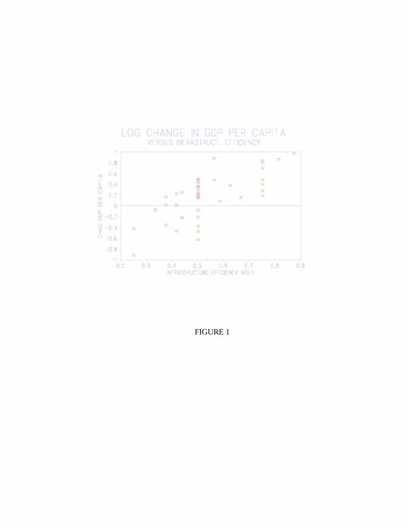
FIGURE 1