infrared spectroscopy of c6d6 - rgn(n=1, 2)
TRANSCRIPT
University of Calgary
PRISM: University of Calgary's Digital Repository
Graduate Studies The Vault: Electronic Theses and Dissertations
2015-02-02
Infrared Spectroscopy of C6D6 - Rgn(n=1, 2)
GEORGE, JOBIN
GEORGE, JOBIN. (2015). Infrared Spectroscopy of C6D6 - Rgn(n=1, 2) (Unpublished master's
thesis). University of Calgary, Calgary, AB. doi:10.11575/PRISM/26528
http://hdl.handle.net/11023/2059
master thesis
University of Calgary graduate students retain copyright ownership and moral rights for their
thesis. You may use this material in any way that is permitted by the Copyright Act or through
licensing that has been assigned to the document. For uses that are not allowable under
copyright legislation or licensing, you are required to seek permission.
Downloaded from PRISM: https://prism.ucalgary.ca

UNIVERSITY OF CALGARY
Infrared Spectroscopy of C6D6 − Rgn(n = 1, 2)
by
Jobin George
A THESIS
SUBMITTED TO THE FACULTY OF GRADUATE STUDIES
IN PARTIAL FULFILLMENT OF THE REQUIREMENTS FOR THE
DEGREE OF MASTER OF SCIENCE
DEPARTMENT OF PHYSICS AND ASTRONOMY
CALGARY, ALBERTA
JANUARY, 2015
© Jobin George 2015
Abstract
The infrared spectra of C6D6 − Rg1,2 complexes were observed, with the rare gas (Rg) being
He, Ne, Ar. The spectra were observed at a resolution of ∼ 60 MHz using a tunable optical
parametric oscillator (OPO) to probe a pulsed supersonic-jet expansion from a slit nozzle.
The detection system also used a balanced subtraction technique to suppress the power
�uctuations inherent to the OPO. Due to a strong Fermi resonance in the C6D
6monomer,
two bands were observed for each of the complexes, one around the vibrational fundamental
of ν12 (≈2289 cm−1) and other around the combination band ν2 + ν13 (≈2275 cm−1) of the
benzene monomer. In the case of C6D
6−Rg dimers, spectra were assigned to a symmetric
top with C6v symmetry with the rare gas atom being located on the C6 symmetry axis.
To observe the C6D
6−Rg
2trimers, the nozzle had to be cooled, resulting in spectra with a
lower rotational temperature. The spectra of the C6D
6−Rg
2trimers were in agreement with
a D6h symmetry structure, where the rare gas atoms are positioned on the C6 symmetry
axis, above and below the C6D
6plane.
i

Acknowledgements
I express my deepest appreciation to my supervisor Dr. Nasser Moazzen-Ahmadi for his
support, persistent help and guidance that made this thesis possible. His enthusiasm and
knowledge of the �eld have been inspirations to me. Working with him in the lab, I learned
the patience and diligence that are necessary for a researcher.
I appreciate the supervisory committee members Dr. David Wesley Hobill, Dr. Brian
Jackel and Dr. Yujun Shi for agreeing to review this thesis. I am very grateful to Dr.
Jalal Norooz-Oliaee and Dr. Mojtaba Razaei for scienti�c support and training. My special
gratitude towards Dr. Bob McKellar for his valuable contributions to the research presented
in this thesis. I am courteous to my supervisor and physics department for �nancial support.
I thank Sahar Sheybani-Deloui for her comments and feedbacks on the thesis. Also,
thanks to my colleagues Mahdi Youse� Koopaei, Luis Welbanks and Aaron Barclay for their
help in the lab and interesting discussions. Gerri, Tracy and Leslie for helping me with the
administration processes. Finally, my family for all of their love and support.
ii

Table of Contents
Abstract . . . . . . . . . . . . . . . . . . . . . . . . . . . . . . . . . . . . . . . . iAcknowledgements . . . . . . . . . . . . . . . . . . . . . . . . . . . . . . . . . . iiTable of Contents . . . . . . . . . . . . . . . . . . . . . . . . . . . . . . . . . . . . iiiList of Tables . . . . . . . . . . . . . . . . . . . . . . . . . . . . . . . . . . . . . . vList of Figures . . . . . . . . . . . . . . . . . . . . . . . . . . . . . . . . . . . . . . viList of Symbols . . . . . . . . . . . . . . . . . . . . . . . . . . . . . . . . . . . . . viii1 Introduction . . . . . . . . . . . . . . . . . . . . . . . . . . . . . . . . . . . 11.1 Generation of van der Waals cluster . . . . . . . . . . . . . . . . . . . . . . . 31.2 Observation of van der Waals cluster . . . . . . . . . . . . . . . . . . . . . . 41.3 Present thesis . . . . . . . . . . . . . . . . . . . . . . . . . . . . . . . . . . . 5
1.3.1 Benzene-(rare gas)n, n=1,2 complexes . . . . . . . . . . . . . . . . . . 51.4 Outline of the thesis . . . . . . . . . . . . . . . . . . . . . . . . . . . . . . . 72 Theoretical Background . . . . . . . . . . . . . . . . . . . . . . . . . . . 92.1 Molecular Hamiltonian . . . . . . . . . . . . . . . . . . . . . . . . . . . . . . 92.2 Rotation-Vibration Hamiltonian . . . . . . . . . . . . . . . . . . . . . . . . . 112.3 Rigid-Rotor and Harmonic Oscillator Approximation . . . . . . . . . . . . . 13
2.3.1 The Principal Moments of Inertia and Rotational Constants . . . . . 142.3.2 Energy levels and wavefunctions of symmetric top rigid-rotor . . . . . 152.3.3 Harmonic Oscillator Schrödinger Equation . . . . . . . . . . . . . . . 17
2.4 Centrifugal Distortion . . . . . . . . . . . . . . . . . . . . . . . . . . . . . . 192.5 Coriolis Coupling . . . . . . . . . . . . . . . . . . . . . . . . . . . . . . . . . 202.6 Absorption line Intensities and Selection rules . . . . . . . . . . . . . . . . . 21
2.6.1 Nuclear spin statistical weights . . . . . . . . . . . . . . . . . . . . . 252.7 Fermi Resonance . . . . . . . . . . . . . . . . . . . . . . . . . . . . . . . . . 263 Experimental Set-up . . . . . . . . . . . . . . . . . . . . . . . . . . . . . 283.1 A Brief Description of the Experimental Set-up . . . . . . . . . . . . . . . . 283.2 Supersonic Jet Expansion . . . . . . . . . . . . . . . . . . . . . . . . . . . . 28
3.2.1 Description of supersonic jet expansion . . . . . . . . . . . . . . . . . 303.2.2 Cluster formation in supersonic jet . . . . . . . . . . . . . . . . . . . 333.2.3 Pulsed Supersonic jet and vacuum set-up . . . . . . . . . . . . . . . . 33
Pulsed valve and nozzle . . . . . . . . . . . . . . . . . . . . . . . . . 33Six-way cross vacuum chamber . . . . . . . . . . . . . . . . . . . . . 34
3.3 Astigmatic Multi-pass Cell . . . . . . . . . . . . . . . . . . . . . . . . . . . . 343.4 Optical Parametric Oscillator probe for van der Waal cluster spectroscopy . 35
3.4.1 Working principles of Optical Parametric Oscillators . . . . . . . . . 363.4.2 The experimental set-up with OPO source . . . . . . . . . . . . . . . 37
Description of the set-up . . . . . . . . . . . . . . . . . . . . . . . . . 37Operation and data acquisition process . . . . . . . . . . . . . . . . . 37Data acquisition software . . . . . . . . . . . . . . . . . . . . . . . . . 40
3.4.3 OPO frequency stabilization . . . . . . . . . . . . . . . . . . . . . . . 403.4.4 SRO-OPO Power �uctuation suppression and background subtraction 42
4 Infrared spectra of C6D6 −Rgn(n = 1,2) . . . . . . . . . . . . . . . . . 44
iii

4.1 Introduction . . . . . . . . . . . . . . . . . . . . . . . . . . . . . . . . . . . . 444.2 Results . . . . . . . . . . . . . . . . . . . . . . . . . . . . . . . . . . . . . . . 45
4.2.1 He1,2 − C6D6 . . . . . . . . . . . . . . . . . . . . . . . . . . . . . . . 474.2.2 Ne1,2 − C6D6 . . . . . . . . . . . . . . . . . . . . . . . . . . . . . . . 504.2.3 Ar1,2 − C6D6 . . . . . . . . . . . . . . . . . . . . . . . . . . . . . . . 51
4.3 Discussion and conclusions . . . . . . . . . . . . . . . . . . . . . . . . . . . . 515 Conclusions . . . . . . . . . . . . . . . . . . . . . . . . . . . . . . . . . . . 57Bibliography . . . . . . . . . . . . . . . . . . . . . . . . . . . . . . . . . . . . . . 60Appendix A Supplementary data for Chapter 4 . . . . . . . . . . . . . . . . . . 64Appendix B Supplementary data for Chapter 4 . . . . . . . . . . . . . . . . . . 84
iv
List of Tables
4.1 Nuclear spin weights of respective symmetries for C6v (dimer) and D6h (trimer) 504.2 Molecular parameters for the C
6D
6
a and C6D
6− Rg complex (in cm−1). Un-
certainties in parenthesis are 1σ from the least-squares �ts in units of the lastquoted digit. . . . . . . . . . . . . . . . . . . . . . . . . . . . . . . . . . . . . 54
4.3 Molecular parameters for the C6D
6and C
6D
6−Rg
2complex (in cm−1). Un-
certainties in parenthesis are 1σ from the least-squares �ts in units of the lastquoted digit. . . . . . . . . . . . . . . . . . . . . . . . . . . . . . . . . . . . . 55
4.4 E�ective intermolecular distances for Rg1,2-benzene in Å . . . . . . . . . . . 554.5 Vibrational shift relative to C6D6 vibration in cm-1 . . . . . . . . . . . . . . 56
A.1 Observed transitions in the ν2 + ν13 (∼ 2275 cm−1) and ν12 (∼ 2288 cm−1)bands of C
6D
6−He (values in cm−1). . . . . . . . . . . . . . . . . . . . . . . 64
A.2 Observed transitions in the ν2 + ν13 and ν12 bands of C6D
6−Ne. . . . . . . . 69
A.3 Observed transitions in the ν2 + ν13 and ν12 bands of C6D
6−Ar. . . . . . . . 75
B.1 Observed transitions in the ν2 + ν13 (∼ 2275 cm−1) and ν12 (∼ 2288 cm−1)bands of C
6D
6−He
2. . . . . . . . . . . . . . . . . . . . . . . . . . . . . . . . 84
B.2 Observed transitions in the ν2 + ν13 and ν12 bands of C6D
6−Ne
2. . . . . . . . 87
B.3 Observed transitions in the ν2 + ν13 and ν12 bands of C6D
6−Ar
2. . . . . . . . 89
v
List of Figures and Illustrations
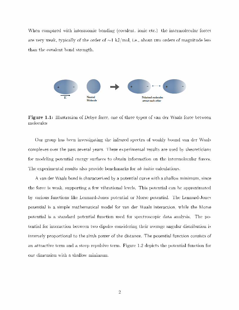
1.1 Illustration of Debye force, one of three types of van der Waals force betweenmolecules . . . . . . . . . . . . . . . . . . . . . . . . . . . . . . . . . . . . . 2
1.2 Typical Lennard-Jones potential function for a van der Waals bond. Wherer is the intermolecular distance, ε is the depth of the potential well and σ isthe intermolecular separation when u(r) = 0 . . . . . . . . . . . . . . . . . . 3
1.3 Illustration of electronic, vibrational and rotational molecular energy levelsand absorption frequencies associated with their transitions. . . . . . . . . . 5
1.4 Experimentally derived structures of C6D
6−Rg, C
6D
6−Rg
2clusters. Rare
gas(Rg) in blue is on the C6 symmetry axis of the Benzene ring . . . . . . . 8
2.1 Figure shows few vibrational levels of the harmonic potential (red trace) andMorse potential (blue). The anharmonicity is taken into account in the real-istic Morse potential. The units are arbitrary . . . . . . . . . . . . . . . . . . 19
3.1 Schematic of the experimental set-up for van der Waal cluster spectroscopy.Probe beam is separated into four channels: jet, reference gas, etalon and afourth channel for background. Jet signal records the absorption spectra ofclusters. All channels are recorded simultaneously. The astigmatic multipasscell increases the e�ective optical path length of the probe laser beam throughthe supersonic cluster stream, hence enhances the signal-to-noise ratio. . . . 29
3.2 Illustration of the supersonic jet expansion of the gas from a nozzle. High pres-sure inside the reservoir gives rise to many collisions near the nozzle openingduring the expansion. Consequently these collisions transfer momentum intothe direction downstream. The zone of silence is the collision free region, themach disk is shock front perpendicular to the �ow. The velocity distributionbefore and after the expansion is shown at the bottom of the �gure . . . . . 31
3.3 Pulsed slit nozzle and cold jacket con�guration inside the vacuum chamber. . 343.4 Schematic of the astigmatic multipass absorption cell with van der Waals
cluster formation in the cell. The laser beam enters in an o�-axis directionand exits at an angle from the input direction. The astigmatic mirror withthe coupling hole with CaF
2window at Brewster angle. . . . . . . . . . . . . 35
3.5 Schematic of the OPO module showing the MgO doped Periodically PoledLithium Niobate crystal (MgO:PPLN) with fanned out grating, the DFB �berlaser and Fiber ampli�er as the pump for the OPO. . . . . . . . . . . . . . . 38
3.6 Illustration of the OPO experimental set-up. Laser beams are shown withsolid yellow lines, data signals with black lines, and synchronizing signalswith dotted lines. . . . . . . . . . . . . . . . . . . . . . . . . . . . . . . . . . 39
3.7 Schematic diagram illustrating the timing sequence for data acquisition inOPO set-up [12]. The red dotted lines shows the counter 2 and 3 are triggeredby counter 1 . . . . . . . . . . . . . . . . . . . . . . . . . . . . . . . . . . . . 40
vi
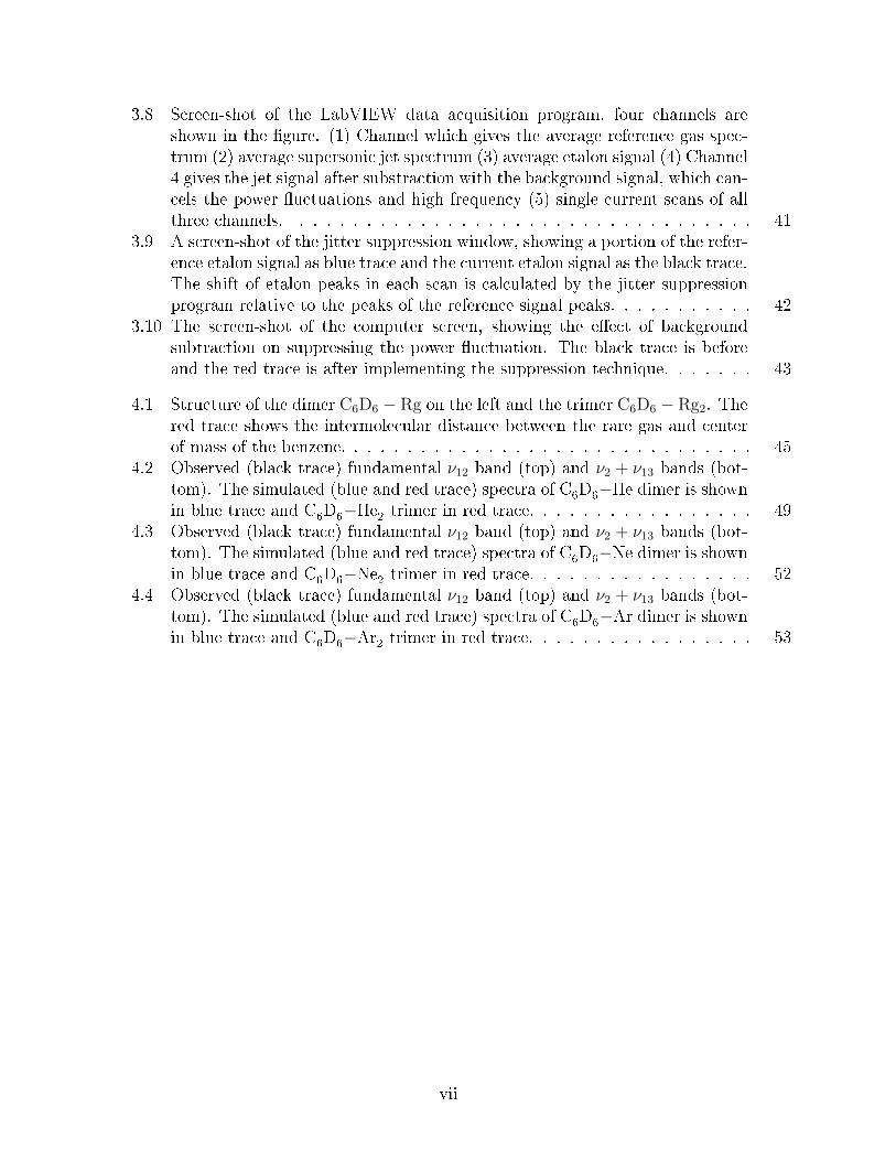
3.8 Screen-shot of the LabVIEW data acquisition program, four channels areshown in the �gure. (1) Channel which gives the average reference gas spec-trum (2) average supersonic jet spectrum (3) average etalon signal (4) Channel4 gives the jet signal after substraction with the background signal, which can-cels the power �uctuations and high frequency (5) single current scans of allthree channels. . . . . . . . . . . . . . . . . . . . . . . . . . . . . . . . . . . 41
3.9 A screen-shot of the jitter suppression window, showing a portion of the refer-ence etalon signal as blue trace and the current etalon signal as the black trace.The shift of etalon peaks in each scan is calculated by the jitter suppressionprogram relative to the peaks of the reference signal peaks. . . . . . . . . . . 42
3.10 The screen-shot of the computer screen, showing the e�ect of backgroundsubtraction on suppressing the power �uctuation. The black trace is beforeand the red trace is after implementing the suppression technique. . . . . . . 43
4.1 Structure of the dimer C6D6 − Rg on the left and the trimer C6D6 − Rg2. Thered trace shows the intermolecular distance between the rare gas and centerof mass of the benzene. . . . . . . . . . . . . . . . . . . . . . . . . . . . . . . 45
4.2 Observed (black trace) fundamental ν12 band (top) and ν2 + ν13 bands (bot-tom). The simulated (blue and red trace) spectra of C
6D
6−He dimer is shown
in blue trace and C6D
6−He
2trimer in red trace. . . . . . . . . . . . . . . . . 49
4.3 Observed (black trace) fundamental ν12 band (top) and ν2 + ν13 bands (bot-tom). The simulated (blue and red trace) spectra of C
6D
6−Ne dimer is shown
in blue trace and C6D
6−Ne
2trimer in red trace. . . . . . . . . . . . . . . . . 52
4.4 Observed (black trace) fundamental ν12 band (top) and ν2 + ν13 bands (bot-tom). The simulated (blue and red trace) spectra of C
6D
6−Ar dimer is shown
in blue trace and C6D
6−Ar
2trimer in red trace. . . . . . . . . . . . . . . . . 53
vii

List of Symbols, Abbreviations and Nomenclature
vdW van der Waals
Rg Rare gas
He Helium
Ne Neon
Ar Argon
C6H
6 Benzene
C6D
6 Deuterated Benzene
ν Vibrational frequency
Dimer Two monomer complex
Trimer Three monomer complex
OPO Optical Parametric Oscillator
SRO Singly Resonant Optical parametric oscillator
IR Infrared
UV Ultraviolet
N2O Nitrous Oxide
N2
Molecular Nitrogen
CO2 Carbon Dioxide
TTL Transistor−transistor Logic
DAQ Data Acquisition card
PZT Lead Zirconate Titantate
PPLN Periodically Poled Lithium Niobate
MgO Magnesium Oxide
CaF2 Calcium Fluoride
viii

DFB Distributed Feedback
PMIFST Principal Moment of Inertia From Structure
A, B, C Rotational constants of the molecule
DJK , DJ Centrifugal distortion constants
ζ Coriolis coupling constant
Ref. Reference
ix

Chapter 1
Introduction
In 1873, a modi�ed version of the ideal gas law was proposed by Johannes Diderik van
der Waals in order to �t the behaviour of real gases in all temperatures and pressures.
The real gases deviate from the ideal gas owing to the �nite size of molecules and the
intermolecular interaction. The pressure of a gas in a container is lower than the pressure
calculated from the ideal gas law due to the intermolecular attraction. All intermolecular
interactions are regarded as van der Waals forces. These forces are responsible for bulk
properties of simple molecules to complex polymers. Van der Waals forces are responsible
for the fundamental properties of matter like melting and boiling points, surface tension,
vapour pressure, etc. These forces are also responsible for shapes acquired by synthetic and
biological macromolecules. Investigating these forces will shed light into the less understood
condensation pathways from molecules in the gas phase to liquid or solid phase. When being
cooled down all gases condense to become liquid or solid. The condensation path begins with
the formation of molecular clusters, which is simply a �nite collection of molecules bound
together by van der Waals force.
The molecules involved in the cluster formation can be polar or non polar. There are three
types of interactions that are responsible for van der Waals forces. The attractive or repulsive
interactions among molecules with permanent dipole moment are called Keesom interactions.
A molecule with a permanent dipole moment, otherwise termed as polar molecule can induce
a dipole moment on a non-polar molecule. The attractive force between the polar molecule
and the non-polar molecule is known as the Debye force (Figure 1.1). The third is the
London dispersion force resulting from the attractive force between any molecules (polar or
non-polar), where the induced dipole moment of the interacting molecules are instantaneous.
1
When compared with interatomic bonding (covalent, ionic etc.) the intermolecular forces
are very weak, typically of the order of ∼1 kJ/mol, i.e., about two orders of magnitude less
than the covalent bond strength.
Figure 1.1: Illustration of Debye force, one of three types of van der Waals force betweenmolecules
Our group has been investigating the infrared spectra of weakly bound van der Waals
complexes over the past several years. These experimental results are used by theoreticians
for modeling potential energy surfaces to obtain information on the intermolecular forces.
The experimental results also provide benchmarks for ab initio calculations.
A van der Waals bond is characterized by a potential curve with a shallow minimum, since
the force is weak, supporting a few vibrational levels. This potential can be approximated
by various functions like Lennard-Jones potential or Morse potential. The Lennard-Jones
potential is a simple mathematical model for van der Waals interaction, while the Morse
potential is a standard potential function used for spectroscopic data analysis. The po-
tential for interaction between two dipoles considering their average angular distribution is
inversely proportional to the sixth power of the distance. The potential function consists of
an attractive term and a steep repulsive term. Figure 1.2 depicts the potential function for
one dimension with a shallow minimum.
2

Figure 1.2: Typical Lennard-Jones potential function for a van der Waals bond. Where ris the intermolecular distance, ε is the depth of the potential well and σ is the intermolecularseparation when u(r) = 0
1.1 Generation of van der Waals cluster
The dissociation energy of van der Waals molecules is comparable to the thermal energy at
room temperature, kBT (∼2.5 kJ mol−1), hence these molecules readily dissociate. Also,
at room temperature molecules typically occupy many thousands of rovibrational states,
making spectroscopy challenging. Therefore, a low temperature condition is required for the
observation of weakly bound clusters, where the molecules can attain very low rotational
temperature.
The supersonic jet expansion technique has been a widely used technique in which the
vibrational, rotational and translational cooling of the gas sample is achieved by an adiabatic
expansion, where the gas at high pressure is allowed to expand into the vacuum through a
pinhole or a slit nozzle. For rotational cooling to occur the pinhole dimension or slit width
3

must be much larger than the mean free path of the particle in the high pressure region.
Consequently, binary collisions of atoms or molecules increases upon entering the vacuum
region and internal energy from rotational and vibrational modes is transferred to a large
extent into the translational energy. This leads to a decrease in rotational and vibrational
temperature, which in turn allows only the lowest ro-vibrational levels of the molecule to
be populated. This compression of the population distribution into the lowest levels greatly
reduces the number of absorbing states. The drastic reduction in spectral congestion and
correspondingly increased signal for the few quantum states which are populated can vastly
simplify spectroscopic analysis.
1.2 Observation of van der Waals cluster
A molecule's internal energy is distributed among electronic, vibrational and rotational en-
ergy (Figure 1.3). The molecular vibrational energy levels correspond to the mid-infrared(IR)
region 2.5-25 µm. Infrared radiation is absorbed when the molecular vibration gives rise to
a net change in dipole moment of the molecule. Consequently, absorption at certain fre-
quencies over the bandwidth of the mid-IR source results in an absorption spectrum. It
should also be noted that not all transitions are allowed due to a set of selection rules (will
be discussed in Chapter 2). When a monochromatic wave of frequency ω and intensity I0
is passed through a sample of absorption path-length L, the intensity transmitted It can be
expressed by Beer-Lambert law It = I0.e−αL, where α is the absorption coe�cient.
Radiation source used in this thesis was a tunable Optical Parametric Oscillator (OPO)
which works on the principle of parametric down conversion and has a bandwidth of 1 MHz.
To obtain the absorption spectrum, the laser beam is passed perpendicular to the gas �ow
and where the cluster concentration is the highest. For a single laser pass the sensitivity or
signal to noise ratio would not be high enough. To enhance the sensitivity, an astigmatic
multi-pass cell is used to make the laser beam pass through the jet around 180 times.
4

Figure 1.3: Illustration of electronic, vibrational and rotational molecular energy levels andabsorption frequencies associated with their transitions.
1.3 Present thesis
The current thesis is concerned with spectroscopic observation and structure determination
of Benzene-noble gas complexes. A dimer with one benzene molecule and one noble gas atom
and a trimer complex with two noble gas atoms and one benzene molecule were observed
and studied. The following sections will explain the motivation behind this study together
with a review of previous studies on complexes containing benzene and noble gases.
1.3.1 Benzene-(rare gas)n, n=1,2 complexes
There is a strong interest among researchers to understand the solvation process of molecules
through the study of van der Waals complexes. It is the weak van der Waals interactions
that lead to solvation phenomena and in�uence the chemical reactivity in solutions. Organic
5
molecule - rare gas complexes have been one of the attractive model for studying solvation,
thus their spectroscopy at high resolution has an extensive history [11]. The �rst rotationally
resolved spectra of vdW complexes in this class, C6H6 − He dimer and C6H6 − (He)2 trimer
were observed in 1978 by Smalley et al. [14] by means of electronic spectroscopy in a super-
sonic jet. The resolution of the UV spectrum was very low due to the large laser bandwidth
of 1.3 GHz. Only a small number of rotational states were populated due to a low rotational
temperature of 0.3 K. Because of the low resolution and a few observed rotational lines, the
deduced rotational constants had limited accuracy. However, by assigning the transitions to
a symmetric top, the structure of the complexes was estimated as a He atom lying above
and/or below the plane of benzene and on the C6 symmetry axis. A recent study in 2013
by M. Hayashi et al. [17] on the same structure at much higher resolution of ∼250 MHz
con�rmed this structure.
In 1992 Neusser et al. [20] observed the complexes of benzene with other rare gas atoms
Ne, Ar, Kr, Xe and also with N2molecule. The spectra were obtained with a resolution
of 120 MHz. All structures were determined to have the same structure as benzene - He
dimer and trimer. Although, the distance between the rare gas atom and the benzene plane
di�er for each complex due to the variation in polarizability of rare gas atoms [17]. The
structures obtained are relatively rigid but when the rare gas atom is replaced with N2, the
structure becomes non rigid because of the internal rotation of the N2molecule around the
C6 symmetry axis of the benzene.
Rotational spectroscopy in the microwave region o�ers much higher resolution, of the or-
der of KHz, and therefore, the structure determined from the deduced rotational parameters
is highly accurate. Until 1990 [29], there was no report on the observation of a complex of
an aromatic molecule with rare gas atom in the microwave region. This was because the
monomers (benzene and rare gas atom) taking part in the formation of the complex have
no permanent dipole moment, and the induced dipole moment of the complex is very small
6

(0.11D). In 1994, Bauder et al. [28] measured the microwave spectra of benzene - Ar and
benzene-1,3,5-d3 - Ar with a resolution of ∼ 40 KHz. The isotopic substitution does not
change the bond length of the molecules and helps to con�rms the structural determination.
So far, there is no observation of benzene - rare gas complexes in the infrared region.
This thesis is based on the infrared observation of C6D6 − (Rg)n (n=1,2) with the rare
gas being He, Ne, or Ar. The spectra were observed in the regions of ν12, C-D stretch
fundamental vibration of C6D
6near 2289 cm−1 and ν2 + ν13 combination band near 2275
cm−1 which are coupled by Fermi resonance, where ν2 is C6D
6ring stretch mode and ν13 is
C6D
6ring stretch deformation mode. Fermi resonance is a phenomena in which an overtone
or a combination band shows an unexpectedly high intensity. This is discussed in some
detail in Chapter 3. For C6D6 − Rg dimers, the spectra were assigned to a symmetric top
with C6v symmetry with the rare gas atom being located on the C6 symmetry axis. The
C6D6 − (Rg)2 trimers were in agreement with a D6h symmetry structure, where the rare
gas atoms are positioned above and below the C6D
6plane. These structures were already
determined using the microwave and electronic spectroscopy [11] except for the C6D6 − (Ne)2
trimer. The rotational temperature of trimer spectra were found to be 1.3K. The spectra
were observed at a resolution of ∼ 60 MHz, which is almost 20 times higher than the �rst
benzene-rare gas complex observation [46].
1.4 Outline of the thesis
The focus of this thesis is on the observation of Benzene-rare gas dimer and trimer com-
plexes in a pulsed supersonic jet apparatus with a continuous wave OPO as probe laser. The
thesis has �ve chapters. Chapter 2 contains an introduction to the theoretical background
necessary for the experiment and the analysis of the observed spectrum. The molecular
Hamiltonian is introduced and the solutions of the lowest order approximation for rotation-
vibration Hamiltonian are presented. The experimental arrangement used for the spectral
7

Figure 1.4: Experimentally derived structures of C6D
6−Rg, C
6D
6−Rg
2clusters. Rare
gas(Rg) in blue is on the C6 symmetry axis of the Benzene ring
measurement is described in Chapter 3. In this chapter, production of cold molecular beam
through supersonic-jet expansion technique, implementation of OPO as probe laser and
suppression of power �uctuation is discussed in details. In Chapter 4 the results of the
experimental spectra of Benzene-rare gas clusters, the molecular parameters and the corre-
sponding structure of the complexes are presented. Finally, Chapter 5 discuss the conclusion
of the experimental studies and future prospectives.
8
Chapter 2
Theoretical Background
In this chapter, the theory required for analysing the spectroscopic results from the ex-
periment is discussed. The lowest order approximation for the rotational and vibrational
Hamiltonian are deduced by modelling the molecule as a combined rigid rotor and har-
monic oscillator. The observed van der Waals clusters in this thesis are symmetric top. The
rovibrational wavefunctions and energies for rigid symmetric top molecules are presented.
2.1 Molecular Hamiltonian
To treat rovibrational spectra a molecular Hamiltonian must be developed. A molecule is
composed of nuclei and electrons that are held together by electrostatic interactions. Thus,
the molecular Hamiltonian operator H will have the properties of nuclei and electrons. The
energies of the molecular system are determined by the eigenvalues of the time-independent
Schrödinger equation
HΦ = EΦ, (2.1)
where the Hamiltonian H can be written as
H = TCM + Tint + V + Hes + Hhfs. (2.2)
In Equation 2.2, TCM is the kinetic energy of the center of mass with respect to an arbitrary
space �xed system of axes. The second term Tint is the sum of the kinetic energy of all
particles (electrons and nuclei), which is also the intramolecular kinetic energy with respect
to a molecule �xed axes system with the origin at the molecular center of mass. The terms
in V represent the electrostatic potential energy between the electrons and the nuclei, Hes is
the interaction energy of the electron spin magnetic moment and Hhfs is the interaction due
9
to the nuclear magnetic and electric moments. In Equation (2.2) one needs to consider only
the internal dynamics of the molecule with respect to the molecule �xed axes system. Since
any motion with respect to an arbitrary space �xed axes leaves the molecular Hamiltonian
invariant. We write 2.2 as
H = TCM + Hint (2.3)
Hint = Hrve + Hes + Hhfs (2.4)
where the spin-free rovibronic Hamiltonian Hrve is
Hrve = Tint + V (2.5)
Hint can be approximated to Hrve, for molecules in their singlet electronic ground states
with unresolved nuclear hyper�ne structure. This approximation is the starting point of any
molecular energy calculation. The terms discarded, Hes and Hhfs, are extra terms that give
rise to energy level shifts, �ne and hyper�ne structures. Thus, the rovibronic Schrödinger
equation is given by
HrveΨrve = ErveΨrve (2.6)
Solving the rovibronic Schrödinger equation (Equation (2.6)) is quite di�cult. The direct
numerical method would require enormous computational resources. However, it is practical
to use indirect methods, which involves making approximations to simplify the Hamiltonian
to an extent where the associated Schrödinger equation can be solved rather easily. One
of the main approximation among these is the Born-Oppenheimer approximation. This is
based on the fact that the electronic motion is so fast in comparison with the nuclear motion
that the electronic energy reaches its equilibrium value at each instant. Thus one can treat
the vibration and rotation of the nuclei separate from the electronic motion. Thus Hrve
becomes
Hrve = He + Hrv. (2.7)
As a result, the rovibronic Schrödinger equation is solved by �rst solving the electronic
Schrödinger equation at many �xed geometries and then solving the rotation-vibration
10

Schrödinger equation for the nuclei. Transitions involved in this thesis are among the
rotational-vibrational states in the ground electronic state, so only the rotation-vibration
Hamiltonian is considered.
Rigid rotor and harmonic oscillator approximations are made for solving the rotation-
vibration Schrödinger equation where the resulting equation is separated into the rotation
and vibration parts. Here, the rotational part is the rigid rotor wavefunction expressed
in Euler angles whereas the vibrational wavefunction is the product of (3N-6) harmonic
oscillator wavefunctions (for linear molecule this is 3N-5), where N is the number of nu-
clei. For the above approximations it is required to �nd the appropriate coordinates for
the Schrödinger equation. Several coordinate system are introduced for the separation of
various molecular motions. The general Hamiltonian in Equation (2.5) is set up in a space
�xed axes system, (X, Y, Z). For the separation of rotation and vibration parts of the
Schrödinger equation, which enables to understand the rovibrational spectra of a molecule,
an axes system (x, y, z) is introduced with the origin at the nuclear center of mass of the
molecule. The rovibrational Hamiltonian is then expressed using the coordinates (θ, φ, χ) and
(Q1, Q2, . . . , Q(3N−6)). Where, (θ, φ, χ) are the Euler angles which de�ne the orientation of
the (x, y, z) axes frame with respect to the (X, Y, Z) axes frame; and the (Q1, Q2, . . . , Q(3N−6))
are the normal vibrational coordinates of the molecule.
2.2 Rotation-Vibration Hamiltonian
A detailed derivation procedure of rotation-vibration Hamiltonian is given by Bunker and
Jensen [1]. The rovibrational Hamiltonian is expressed in terms of the angular momentum
operator J , normal coordinates Qr, their conjugate momenta Pr = −i~∂/∂Qr. With Born-
Oppenheimer approximation the Hamiltonian is given by
11

Hrv =1
2
∑α
µeααJ2α +
1
2
3N−6∑r
(P 2r + ωrQ
2r), (2.8)
+1
2
∑α,β
(µαβ − µeαβ)(Jα − pα)(Jβ − pβ), (2.9)
−∑α
µeααJαpα +1
2
∑α
µeααp2α, (2.10)
− ~2
8
∑α
µαα +1
6
∑r,s,t
ΦrstQrQsQt +1
24
∑r,s,t,u
ΦrstuQrQsQtQu + · · · . (2.11)
where α and β are x, y, and z. µ is the inverse of the moment of inertia matrix and
superscript e stands for a molecule in the equilibrium con�guration. µαβ in Equation 2.9
are the elements of µ, which is the inverse matrix of the instantaneous inertia matrix, and
µeαβ in Equations 2.8 and 2.10 are the elements of the matrix µe which is the inverse of the
moment of inertia matrix for the molecule in its equilibrium con�guration. Jα and Jβ are
referred to as the components of rovibronic angular momentum operators on the molecule's
�xed axes, and pα and pβ are components of the vibrational angular momentum operator,
with pα given by
pα =∑r,s
ζαr,sQrPs (2.12)
where ζαr,s are the Coriolis coupling constants. λr, Φrst, and Φrstu in Equations 2.8 and
2.11 are the terms with force constants which comes from the the Taylor expansion of the
potential energy VN in the normal coordinates Qr,
VN =1
2
∑r
λrQ2r +
1
6
∑r,s,t
ΦrstQrQsQt +1
24
∑r,s,t,u
ΦrstuQrQsQtQu + · · · . (2.13)
and the vibrational kinetic energy operator takes the form
Tvib =1
2
∑r
P 2r (2.14)
The �rst term of the rovibrational Hamiltonian (Equation 2.8) is the sum of Hamiltonian
(Hrot) of the rigid rotor and the second term is the sum of 3N−6 harmonic oscillator Hamil-
tonians (Hvib). The third term (Equation 2.9) is responsible for the centrifugal distortion,
12
and the terms in Equations 2.10 and 2.11 are due to vibrational Coriolis coupling and an-
harmonicity, respectively. The anharmonicity results in higher order e�ects such as Fermi
interactions.
2.3 Rigid-Rotor and Harmonic Oscillator Approximation
To solve the rovibrational Schrödinger Equation 2.6, we consider the lowest order of approx-
imation, the rigid rotor approximation in which the molecule is treated as a rigid-rotor and
harmonic oscillator approximation where the molecular vibrations is considered as a sys-
tem composed of 3N − 6 independent harmonic oscillators. Thus we can write approximate
rovibronic Hamiltonian as
H0rv =
1
2
∑α
µeααJ2α︸ ︷︷ ︸
Hrot
+3N−6∑r
1
2(P 2
r + ωrQ2r)︸ ︷︷ ︸
Hvib
(2.15)
and the rotation-vibration Schrödinger equation is
H0rvΨ0
rv = E0rvΨ0
rv (2.16)
where Ψ0rv is the wave functions of the rotation-vibration Hamiltonian given by
Ψ0rv = Ψrot(θ, φ, χ) Ψv1(Q1)Ψv2(Q2) · · ·︸ ︷︷ ︸
Ψvib(Q1,Q2,··· ,Q(3N−6))
(2.17)
and the eigenvalues or energies
E0rv = Erot + Ev1 + Ev2 + · · ·+ Ev(3N−6)︸ ︷︷ ︸
Evib
(2.18)
where
[1
2
∑α
µeααJ2α]Ψrot = ErotΨrot (2.19)
and
[3N−6∑r
1
2(P 2
r + λrQ2r)]Ψvr = EvrΨvr (2.20)
Equation 2.19 is the rigid-rotor Schrödinger equation and Equation 2.20 is the harmonic
oscillator Schrödinger equations, respectively.
13

2.3.1 The Principal Moments of Inertia and Rotational Constants
In order to simplify the rotational kinetic energy for the equilibrium nuclear con�guration
of the molecule we choose the orientation of the molecule �xed (x, y, z) axes as the principal
axes of inertia. The moment of inertia matrix I of a rigid body can be written as
I =
Ixx Ixy Ixz
Iyx Iyy Iyz
Izx Izy Izz
(2.21)
where the diagonal elements are
Iαα =∑i
mi(β2i + γ2
i ) (2.22)
where α,β,γ, is a permutation of x, y, z, and mi are the atomic masses. The o�-diagonal
elements are
Iαβ = −∑i
miαiβi. (2.23)
The rotational Hamiltonian of a molecule is developed in a way that the x, y, z molecule-�xed
frame is attached to the molecule so that they align with the principal axes. The x, y, z prin-
cipal axes makes the o�-diagonal elements Iαβ vanish and the diagonal elements are termed
as the principal moments of inertia. The principal axes of the equilibrium con�guration of
molecule are labelled as a, b and c, the labelling scheme is in the sequence of increasing value
of the moment of inertia, i.e.
Ia ≤ Ib ≤ Ic (2.24)
Molecules are classi�ed in �ve groups based on (Equation (2.24)). These are:
- Linear molecule, Ib = Ic, Ia = 0; example, N2O.
- Prolate symmetric top, Ia < Ib = Ic; example, CH3Cl.
- Oblate symmetric top, Ia = Ib < Ic; example, C6H
6.
14

- Spherical top molecule, Ia = Ib = Ic; example,CH4.
- Asymmetric top molecule, Ia < Ib < Ic; example, H2O.
Usually, spectroscopic data are tabulated in units of wavenumber (cm−1). The rigid-rotor
Hamiltonian (from Equation 2.15) in cm−1 can be written in the principal axes frame (a, b, c)
as
Hrot =1
2
∑α
µeααJ2α = ~−2
(AJ2
x +BJ2y + CJ2
z
)(2.25)
where the rotational constants are given by
A =~
4πcIa, B =
~4πcIb
, C =~
4πcIc(2.26)
where ~ is the Planck constant and c is the speed of light. From Equation 2.24 the rota-
tional constants must be in the order of A ≥ B ≥ C. The eigenvalues of the rotational
Hamiltonian depend on the rotational constants. The rotational constants depend on the
principal moments of inertia, which, in turn depend on the atomic masses, bond angles and
bond length of the molecule. Hence, the structure of the molecular system is determined
from the rotational constants.
2.3.2 Energy levels and wavefunctions of symmetric top rigid-rotor
The van der Waals complexes observed in this thesis are symmetric top molecular systems,
so only energy levels and wavefunctions of the symmetric top molecule are discussed here.
For an oblate top the c-axis is chosen as the z-axis, where the z-axis is the molecular
symmetry axis. In the case of prolate tops, the symmetry axis is the a-axis. The commutation
relations between Hrot and angular momentum operators [13] for an oblate top molecule is
given by,
[Hrot, J2] = [Hrot, JZ ] = [Hrot, Jc] = 0, (2.27)
This implies that Hrot, J2, JZ , and Ja/c share a simultaneous set of eigenfunctions which
are represented as |J, kc,m〉 for an oblate top and |J, ka,m〉 for a prolate top, and the
15
corresponding eigenvalue equations are
Hrot|J, kc,m〉 = Erot|J, kc,m〉 (2.28)
J2|J, kc,m〉 = J(J + 1)|J, kc,m〉 (2.29)
JZ |J, kc,m〉 = m|J, kc,m〉 (2.30)
Jc|J, kc,m〉 = kc|J, kc,m〉 (2.31)
where kc is the quantum number associated with the projection of the total angular mo-
mentum onto the molecular �xed axis and the quantum number m is the projection on the
symmetry axis �xed in space and it can take the following values,
kc = J, J − 1, . . . ,−J + 1,−J (2.32)
m = J, J − 1, . . . ,−J + 1,−J (2.33)
and the eigenfunction
|J, kc,m〉 = (−1)m−kc
√2J + 1
8π2DJ−m,−kc(φ, θ, χ). (2.34)
DJm,kc(φ, θ, χ) are proportional to the elements of Wigner's rotation matrix, [6], where
DJm,kc(φ, θ, χ) = 〈J,m|R(φ, θ, χ)|J, kc〉, (2.35)
where R(φ, θ, χ) is the rotation operator given by
R(φ, θ, χ) = e−iφJZe−iθJY e−iχJc . (2.36)
From Equations (2.25) and (2.28) - (2.31), rotational energy levels can be obtained for
an oblate top.
Hrot|J, kc,m〉 =(AJ2
a +BJ2b + CJ2
c
)|J, kc,m〉 (2.37)
=(AJ2
a −BJ2c +BJ2
c +BJ2b + CJ2
c
)|J, kc,m〉 (2.38)
=(BJ2 + (C −B)J2
c
)|J, kc,m〉 (2.39)
16
Therefore,
Erot(J, kc) = BJ(J + 1) + (C −B)k2c . (2.40)
Similarly, the energy levels for prolate tops are
Erot(J, ka) = BJ(J + 1) + (A−B)k2a. (2.41)
From Equation (2.33) it is obvious that for each J value there are (2J + 1) di�erent kc states
corresponding to the di�erent possible projections of J on the molecular symmetry axis.
Each (J, kc) level then has (2J + 1) di�erent m levels corresponding to projections of J on
the space �xed axes. For k 6= 0, each level is 2(2J + 1)-fold degenerate since states with ±ka
having the same energy, whereas the level with k = 0 has a degeneracy of (2J + 1)-fold.
The second term of Equation 2.40 is negative for oblate tops hence the rotational energy
decreases with increasing kc. The wavefunctions of prolate and oblate tops serve as basis
function for the asymmetric top molecule.
2.3.3 Harmonic Oscillator Schrödinger Equation
The second term in Equation 2.15 is the vibrational Hamiltonian for N atomic nuclei. The
harmonic oscillator Schrödinger equation for the molecular system is
[3N−6∑r
1
2(P 2
r + ωrQ2r)]Ψv = EvrΨvr (2.42)
For a single mode of vibration this is(1
2(P 2
r + ωrQ2r)
)Φv(Qr) = EvΦv(Qr) (2.43)
where Q is the normal coordinate and P the conjugate momentum. The eigenvalues obtained
from the above equation is
Ev =
(v +
1
2
)~ω, (2.44)
and the eigenfunctions are
Ψv = Nve−ωQ2/2~Hv(
√ω
~Q). (2.45)
17

The Hv(√
ω~Q) is the Hermite polynomial of degree v and Nv is the normalization constant
given by
Nv =
( √ω√
~π2vv!
) 12
. (2.46)
Now, the eigenvalues of Equation 2.42 with all modes of vibration becomes
Evib =3N−6∑r=1
(vr +
1
2
)~ωr. (2.47)
The vibrational eigenfunction for the molecule can be written as the product of the eigen-
functions for each of the normal coordinates,
Ψvib = Ψv1(Q1)Ψv2(Q2) · · ·Ψv3N−6(Q3N−6)
= exp
[−1
2
3N−6∑r=1
ωr~Q2r
]3N−6∏r
NvrHvr(
√ωr~Qr), (2.48)
Based on the degeneracies of the normal modes, the complete vibrational wavefunctions of
a molecule is written as a product of one-, two- or three- dimensional harmonic oscillator
functions.
Anharmonicity
The experimental studies of molecular spectra and calculations on simple molecular systems
have shown that the general vibration potential function is anharmonic in nature. The har-
monic oscillator model does not include the anharmonicity and the dissociation limit. Morse
potential function is a practical function used for simulating the vibrations between two nuclei
in a molecule. Morse potential includes anharmonicity and at larger internuclear distance,
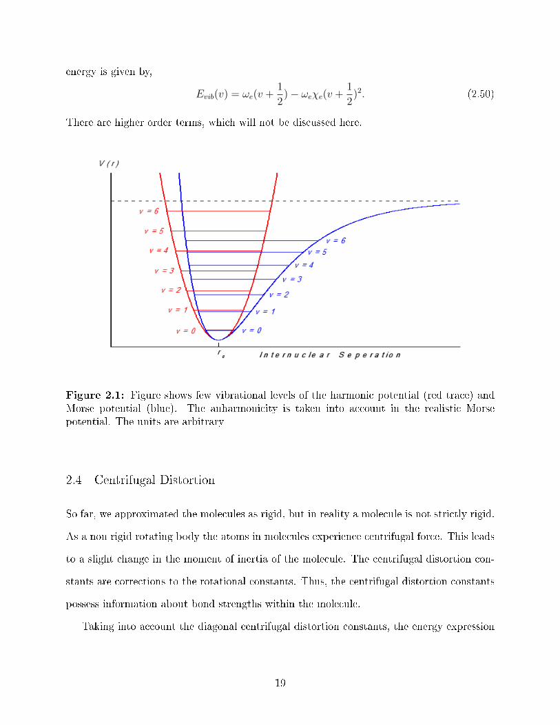
it asymptotically approaches a dissociation limit. Figure 2.1 shows the vibrational energy
levels for the �rst few levels of Harmonic oscillator and Morse Potential. The anharmonicity
e�ects becomes signi�cant for higher vibrational quantum number.
Vv(r) = D(1− e−α(r−re)
)2. (2.49)
where D is the dissociation energy of the molecule, re is the equilibrium nuclear distance.
Taking into account the cubic term in the expansion of the potential function the vibrational
18
energy is given by,
Evib(v) = ωe(v +1
2)− ωeχe(v +
1
2)2. (2.50)
There are higher order terms, which will not be discussed here.
Figure 2.1: Figure shows few vibrational levels of the harmonic potential (red trace) andMorse potential (blue). The anharmonicity is taken into account in the realistic Morsepotential. The units are arbitrary
2.4 Centrifugal Distortion
So far, we approximated the molecules as rigid, but in reality a molecule is not strictly rigid.
As a non rigid rotating body the atoms in molecules experience centrifugal force. This leads
to a slight change in the moment of inertia of the molecule. The centrifugal distortion con-
stants are corrections to the rotational constants. Thus, the centrifugal distortion constants
possess information about bond strengths within the molecule.
Taking into account the diagonal centrifugal distortion constants, the energy expression
19
for a prolate top becomes
Erot(J, kc) = BJ(J + 1) + (C −B)k2c −DJ [J(J + 1)]2 −DJKJ(J + 1)k2
c −DKk4c , (2.51)
whereDJ , DJK andDK are distortion constants of order B2/ω, ω is the molecular vibrational
frequency. The values of distortion constants are many orders of magnitude smaller than
the rotational constants B and C. The frequency for an R-branch transition J → J + 1,
4K = 0 is given by
ν = Erot(J + 1, K)− Erot(J,K)
= 2(B −DJKk2c )(J + 1)− 4DJ(J + 1)3 (2.52)
where K is the absolute value of kc. In the absence of centrifugal distortions, rotational
transitions are equally spaced and for a given lower state value of J all transitions with
di�erent values of K have identical frequencies. For pure rotational transitions the selection
rule is ∆K = 0, K dependent terms in Equation 2.51 disappears, it is therefore not possible
to determine the A or C constants. For the rovibrational transitions with the selection rule
∆K = ±1 (Section 2.6), it is possible to determine A or C in the ground or excited state.
2.5 Coriolis Coupling
The Coriolis forces are responsible for the coupling of di�erent normal vibrational modes via a
rotational degree of freedom. The Coriolis coupling can also occur between the components of
the degenerate vibrational mode, for example coupling of degenerate C-H stretching modes
in benzene [8]. In the lowest order, the degenerate vibrational modes are treated as a
two-dimensional isotropic harmonic oscillator, with the energy of the mode given by Ev =
(v + 1)~ω.
Because the motion of the atoms in a degenerate vibrational mode is perpendicular to
the molecular axis, the vibrational angular momentum pv = ζvlv generated is along the
molecular axis, where lv, the vibrational angular momentum quantum number, can have
20

values between v to −v in steps of 2 and |ζ| is the coupling constant which varies between
0 and 1. Taking into account the vibrational angular momentum, the quadratic part of the
rotational Hamiltonian of the symmetric top becomes [7]
Hrot = B(J2x + J2
y ) + C(J2z − pv)2 (2.53)
Substituting for pv and expanding the above equation, we get
Hrot = B(J2x + J2
y ) + CJ2z − 2CJzζvlv = (C −B)J2
z +BJ2 − 2CJzζvlv (2.54)
where the term C(ζvlv)2 is neglected, since it is purely vibrational and does not a�ect the
rotational state. Now, the energies of the Hamiltonian is given by,
Erot = BJ(J + 1) + (B − C)k2c − 2Ckcζlv (2.55)
where the term 2Ckcζlv represents the contribution of the Coriolis coupling. The Coriolis
coupling splits the energy levels, since k and l can take positive or negative values in Equa-
tion 2.55.
There is also a small but measurable contribution from the higher order terms in the rovi-
brational Hamiltonian. The most important among these is referred to as l-doubling, which
is due to the operator given by,
Hld =1
4qv
(J2
+q2v− + J2
−q2v+
)(2.56)
where J± = Jx ± iJy and qv± = qv,a ± iqv,b are ladder operators, subscripts a and b indicate
the two components of the degenerate mode. The �rst term in Equation 2.56 lowers the k
and lv quantum number by 2 and the second term raises both quantum numbers by 2. The
coupling of the degenerate vibrational modes occurs in the same plane.
2.6 Absorption line Intensities and Selection rules
Consider a monochromatic radiation with an intensity I0 and wavenumber ν travelling a
distance l through a sample with concentration c∗. The transmitted intensity according to
21
the Beer-Lambert law is given by,
I(ν) = I0(ν)e−lc∗σ(ν) (2.57)
where σ(ν) is the absorption coe�cient. The absorption coe�cient is a measure of the extent
to which the initial intensity is absorbed. Molecules absorb or emit infrared radiation when
the vibration of the molecule give rises to a change in the electric dipole moment, µ.
Considering that molecules are in thermal equilibrium at an absolute temperature of T ,
the intensity of an absorption line is proportional to the fraction of the molecules F (Ei) in
the initial energy state Ei. From Maxwell- Boltzmann Distribution,
Fraction of molecules in level Ei : F (Ei) =gie−Ei/kBT∑
j gje−Ej/kBT
, (2.58)
where kB is the Boltzmann constant, gi is the degeneracy of the state i. F (Ei) varies with
temperature and a sample at a very low temperature has only few of the lowest energy levels
of the molecules are populated hence the spectrum appears much simpler than a sample at
a higher temperature.
Apart from the absorption of radiation, molecules also undergo resonant stimulated emis-
sion. In stimulated emission, a molecule in an excited energy state Ef is stimulated by a
radiation of frequency νif to drop into a lower energy state of Ei. This process reduces the
absorption process by a multiplicative factor given by [3],
Resonant stimulated emission : Rstim(f −→ i) = 1− exp (−hνif/kBT ) (2.59)
In addition to the population of the initial state and stimulated emission, the spectral line
intensity also depends on an intrinsic value called the line strength S(f ←− i). The line
strength depends on the molecular electric dipole moment for the transition between rota-
tional levels and the change in the electric dipole moment for the transition between vibra-
tional levels.The integrated absorption coe�cient for an electric dipole transition between
states with initial energy of Ei and �nal energy of Ef , is given by [1]
I(f ←− i) =
∫Line
σ(ν)dν (2.60)
22

=8π3NAνif
(4πε0) 3hc2F (Ei)Rstim(f −→ i)S(f ←− i) (2.61)
where NA is the Avogadro number, νif = (Ef − Ei)/hc is the frequency of the transition in
cm−1, h is the Planck's constant, c is the speed of light in vacuum, ε0 is the permittivity of
vacuum, and function S(f ←− i) is
Line strength : S(f ←− i) =∑
A=X,Y,Z
|〈Ψ′|µA|Ψ〉|2, (2.62)
where µA (A = X, Y, Z) are the components of the electric dipole moment in the space-�xed
axis and Ψ′ and Ψ are eigenfunctions of the molecular Hamiltonian. Let us express µA in
terms of the components of electric dipole moment in the molecule-�xed frame
µA =∑
α=x,y,z
λAαµα (2.63)
here λ represents the transformation matrix from space �xed to molecular �xed frame, whose
elements are functions of Euler angles, and µα is given by
µα =∑j
ejqαj, (2.64)
where qαj and ej is the coordinate and the charge of the jth particle. The Taylor expansion
series of µα about the equilibrium con�guration of the molecule can be written as
µα = µ0α +
∑l,k
(∂µα∂qαl
)0
qαl +1
2
∑l,k
(∂2µα
∂qαl∂qαk
)0
qαlqαk + · · · . (2.65)
Considering only rovibrational transitions within a given electronic state, the |Ψ〉 can be
taken as the product of |Ψv〉(vibrational) and |Ψrot〉(rotational) wavefunctions. The integral
in Equation 2.62 becomes
〈ψ′vψ′rot|µA|ψvψrot〉 =
Pure rotational︷ ︸︸ ︷∑α
〈ψ′v|ψv〉〈ψ′rot|λAα|ψrot〉µ0α
23

+
Rovibrational︷ ︸︸ ︷∑α
∑l,k
(∂µα∂qαl
)0
〈ψ′rot|λAα|ψrot〉〈ψ′v|qαl|ψv〉
+
Combination and overtones︷ ︸︸ ︷∑α
∑l,k
(∂2µα
∂qαl∂qαk
)0
〈ψ′rot|λAα|ψrot〉〈ψ′v|qαlqαk|ψv〉
+ · · · . (2.66)
The possibility of a transition between any two energy levels is determined by the integrals
in each term of Equation 2.66.
Rotational selection rule
For a given vibrational state, 〈Ψ′v|Ψv〉 = 1, hence pure rotational transitions within a given
vibrational level are governed by the term 〈Ψ′rot|λAα|Ψrot〉 in Equation 2.66. With a perma-
nent dipole moment, i.e. µeqα 6= 0, the rotational matrix elements are
〈Ψ′rot|λAα|Ψrot〉 = 〈J ′, k′,m′|λAα|J, k,m〉 (2.67)
For example, for symmetric top molecules the selection rules for the quantum numbers J, k,
and m in Equation (2.67) are
∆J = ±1, ∆m = 0,±1, ∆k = 0. (2.68)
Rovibrational transitions
The second term in equation 2.66 dictates the rotational transitions between di�erent vi-
brational levels which is relevant for the fundamental vibrations studied in this thesis. The
vibrational matrix elements 〈Ψv′|qαl|Φv〉 gives the vibrational selection rules and the rota-
tional matrix elements 〈Ψ′rot|λAα|Ψrot〉 determine the rotational selection rules. Considering
a symmetric top molecule as an example, there are two kinds of allowed transitions:
(i) Parallel bands: If the transition moment of the vibrational transition is par-
allel to the symmetric top axis or z-axis, the selection rules for the vibrational
24
and rotational quantum numbers are
∆v = ±1, ∆J = 0,±1, ∆k = 0 if k 6= 0,
∆v = ±1, ∆J = ±1, ∆k = 0 if k = 0. (2.69)
(ii) Perpendicular bands: The electric dipole moment variation is in the direc-
tion perpendicular to the top axis and the selection rules are
∆v = ±1, ∆J = 0,±1, ∆k = ±1. (2.70)
Combinations and overtones
The third term and higher orders terms in Equation 2.66 are responsible for the combination
and overtone bands. Since higher derivatives of the dipole moment are much smaller than
the �rst derivative, these bands are normally very weak.
∂2µ/∂Q2 ∼ 0.01µ (2.71)
Typically, combination bands are 50 to 100 times weaker than the fundamental bands.
2.6.1 Nuclear spin statistical weights
The existence of nuclear spin a�ects the population of rotational levels, which explains
certain intensity patterns. For example, molecules with centre of symmetry like CO2, the
odd-J rotational lines in P and R branch have zero intensity. So �nding a statistical weight
of the rovibronic states is necessary for assigning molecular spectra.
The complete internal wavefunction of the molecule Ψint is the product of rovibronic
wavefunction Ψrve and the nuclear spin wavefunction Ψns. A rovibronic state would be
populated (have non zero statistical weight) only if the product of the symmetries of the
Ψrve and Ψns is an allowed symmetry in Ψint. This product forms a basis function for
expressing Ψint.
25

From the Fermi-Dirac and Bose-Einstein statistics, the complete internal wavefunctions
Ψint of the molecule must be invariant under even or odd permutations of bosons (integer
spin) and any even permutation of identical fermions (half integer spin). This means that
sign of Ψint will change only under an odd permutation of identical fermions. These can be
written as,
P(even)Ψint = Ψint, P(odd)Ψint = −Ψint for fermions, (2.72)
P(even/odd)Ψint = Ψint for bosons. (2.73)
In addition to this Ψint can have + or - parity due to the e�ect of inversion operation E∗. E∗
is de�ned as, when applied to a molecule, the operation of inverting the spatial coordinates
of all the nuclei.
E∗Ψint = ±Ψint. (2.74)
Using Equations (2.72) and (2.74), the symmetry of the complete internal wavefunction
can be determined. To form an acceptable basis function for Ψint, the product of the symme-
try species of rovibronic state and the nuclear spin state must contain the symmetry species
for Ψint. This condition explains the missing of certain spectral lines and di�erent statistical
weights for various rovibronic states which give rise to intensity alternations.
2.7 Fermi Resonance
The rotation-vibration Hamiltonian Equations 2.9 to 2.11 shows the terms that introduce
perturbations within an electronic state. These terms are responsible for the interaction
between states that are in resonance (having energies that are close). The perturbations
caused by anharmonicity are introduced by cubic, quartic, quintic, . . ., terms in the expansion
of the potential energy (Equation 2.13). Among these, the cubic potential energy term
gives rise to the interaction between the fundamental vibration and overtone or combination
states. This interaction results in frequency shifts and stealing of intensity from the strong
26

fundamental band to overtone or combination band, the phenomenon is referred as Fermi
resonance. The observation of Fermi resonance is of particular interest in the thesis and is
discussed in the next chapter. When the resonating levels are close in energy, the magnitude
of the energy shift can be obtained. For two resonating levels a and b, the shifted energy λ
is given by the determinant, [4] ∣∣∣∣∣∣∣E0a − λ H ′
H ′ E0b − λ
∣∣∣∣∣∣∣ = 0, (2.75)
where H ′ is the o� diagonal Fermi coupling constant term. The solution of the equation 2.75
is given by,
λ =E0a + E0
b
2± 1
2[4 | H ′ |2 +(E0
a − E0b )
2]1/2 (2.76)
E0a − E0
b is the energy separation of the unperturbed levels. The �rst term gives the mean
energy of the levels. The second term shows that one level is pushed up in energy and the
other down.
In C6D
6, the combination mode (ν2+ν13) and the fundamental mode (ν12) have nearly the
same frequency and are of same symmetry, hence they interact strongly by Fermi resonance.
The cubic potential term in the the Hamiltonian that causes this interaction is,
H′ =1
2K2,12,13Q2Q12Q13 (2.77)
where K2,12,13 is the cubic potential constant. Q2, Q12 and Q13 are the corresponding vibra-
tional coordinates. For C6D
6, the shift due to Fermi resonance between combination mode
(ν2 + ν13) and the fundamental mode (ν12) in equation 2.76 is about ∼ −3.9cm−1.
27
Chapter 3
Experimental Set-up
3.1 A Brief Description of the Experimental Set-up
In this chapter the experimental set-up used to record the spectra is discussed in detail.
Figure 3.1 shows a schematic of the experimental arrangement. Some of the main components
of the system are the supersonic jet expansion, IR laser source, IR detectors, the multipass
cell, transfer optics and the data acquisition. The clusters were generated by a single pulsed
nozzle in a supersonic expansion and were probed using the laser source. The signal to noise
ratio of the absorption spectra is increased by increasing the laser path length through the
supersonic jet. This is done by employing a multipass cell in the vacuum chamber. To
calibrate the observed spectra in frequency, an absorption spectrum of a reference gas at
room temperature and an etalon, with a free spectral range(FSR) of 285 MHz (0.0099 cm−1)
were used. The signals from the jet, reference gas and etalon were recorded.
The following sections will describe the supersonic jet expansion and multipass cell, Opti-
cal Parametric Oscillator and its working principle, and then a detailed discussion of transfer
optics and data acquisition scheme is given.
3.2 Supersonic Jet Expansion
Supersonic jet expansion can provide an almost perfect sample suitable for spectroscopic
studies. The adiabatic jet expansion creates a low temperature environment. The low
temperature is important because (a) it is essential for creating weakly bound van der Waals
clusters which would otherwise dissociate at higher temperature and (b) spectra obtained
are simpli�ed because only the lowest rotational levels in the ground vibrational state are
28
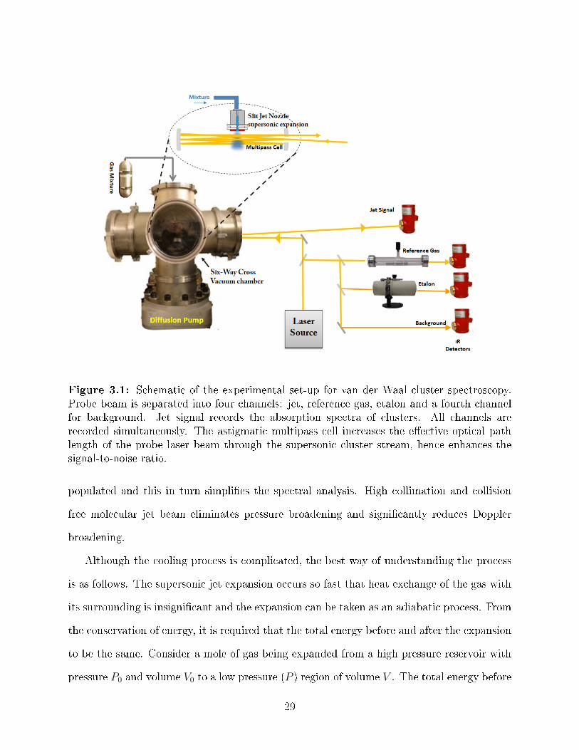
Figure 3.1: Schematic of the experimental set-up for van der Waal cluster spectroscopy.Probe beam is separated into four channels: jet, reference gas, etalon and a fourth channelfor background. Jet signal records the absorption spectra of clusters. All channels arerecorded simultaneously. The astigmatic multipass cell increases the e�ective optical pathlength of the probe laser beam through the supersonic cluster stream, hence enhances thesignal-to-noise ratio.
populated and this in turn simpli�es the spectral analysis. High collimation and collision
free molecular jet beam eliminates pressure broadening and signi�cantly reduces Doppler
broadening.
Although the cooling process is complicated, the best way of understanding the process
is as follows. The supersonic jet expansion occurs so fast that heat exchange of the gas with
its surrounding is insigni�cant and the expansion can be taken as an adiabatic process. From
the conservation of energy, it is required that the total energy before and after the expansion
to be the same. Consider a mole of gas being expanded from a high pressure reservoir with
pressure P0 and volume V0 to a low pressure (P ) region of volume V . The total energy before
29
and after the expansion can expressed as,
U0 + P0V0 +1
2mu2
0︸ ︷︷ ︸before expansion
= U + PV +1
2mu2︸ ︷︷ ︸
after expansion
(3.1)
where, 12mu2 is its kinetic energy of the expanding gas, U = Utr + Uv + Ur is its internal
energy which comprises of the translational (Utr), vibrational (Uv) and rotational energy
(Ur), and PV is its potential energy. Considering the reservoir is in thermal equilibrium,
the average velocity of all the gas molecules u0 is zero. Hence, the kinetic energy of the gas
before the expansion can be neglected. Since, the gas expands into a vacuum, the pressure
P after the expansion is very small. Thus, the potential energy PV of the expanded gas can
also be neglected. We therefore get,
U0 + P0V0 = U +1
2mu2 (3.2)
U0 − U =1
2mu2 − P0V0 =
f
2kB(T0 − T ) (3.3)
where f is the number of degrees of freedom, kB is the Bolzmann constant, T0 and T is
the temperature before and after the expansion. From Equation 3.3 we conclude that a
signi�cant amount of internal energy before the expansion converts into the kinetic energy
of the gas �ow, which becomes possible due to a large number of collisions in the initial
stages of the expansion. The non zero average velocity after the expansion accounts the
directional kinetic energy. The signi�cant decrease in internal energy also corresponds to the
large decrease of temperature.
3.2.1 Description of supersonic jet expansion
As mentioned earlier, in a supersonic jet expansion the stream of gas is allowed to expand
from a high pressure region into the vacuum through a nozzle (Figure 3.2). This is supersonic
since the speed of gas stream surpasses the local speed of sound during expansion. Before
the expansion, the gas is in thermal equilibrium and velocity distribution of the gas obeys
30

Figure 3.2: Illustration of the supersonic jet expansion of the gas from a nozzle. Highpressure inside the reservoir gives rise to many collisions near the nozzle opening during theexpansion. Consequently these collisions transfer momentum into the direction downstream.The zone of silence is the collision free region, the mach disk is shock front perpendicular tothe �ow. The velocity distribution before and after the expansion is shown at the bottom ofthe �gure
Maxwell-Boltzmann distribution. from Equation 3.3 it is evident that during the expan-
sion the thermal energy is converted into directional kinetic energy and this decreases the
temperature of the jet progressively. As shown in Figure 3.2 the collisions and the relative
velocity tend to decrease and the atomic velocity distribution gets narrower and narrower.
Note that more than 99% of the gas mixture is composed of Helium, the seeded molecular
sample is less than 1%. This is because the rare gas molecules like Helium have no internal
degrees of freedom like rotation and vibration, so the energy associated with the internal
degrees of polyatomic molecules can be e�ciently transferred to rare gas molecules.
For an ideal gas expanding adiabatically in reversible conditions, an isentropic equation
31
of state can be used to describe the temperature, pressure and density of the beam as a
function of the scale of the expansion [15] [9].
T
T0
=
(P
P0
) γ−1γ
=
(ρ
ρ0
)γ−1
=1
1 + (γ−1)2M2
(3.4)
where T0, P0 and ρ0 are the temperature, pressure and density before expansion in the
reservoir; T , P and ρ are the same quantities during the expansion; γ is the ratio of the
heat capacity CpCv, Cp is the speci�c heat of ideal gas at constant pressure, Cv is the speci�c
heat at constant volume and M is the Mach number which is the ratio of molecular beam
velocity and the local speed of sound. It is evident from the Equation 3.4 that as the Mach
number increases the temperature, pressure and density decrease with the expansion from
the ori�ce. The increase in Mach number is the result of the conversion of thermal energy into
directed kinetic �ow. Collisions among the molecules are necessary for this process. With
increasing distance from the nozzle the collision frequency decreases and the jet density
and the temperature decreases. Thus the Mach number provides a measure of the local
temperature of the jet [18]. As the collisions decrease with density the Mach number reaches
a �nite value, MT , the terminal Mach number for argon as given by Smalley et al. [15] is,
MT = 133(P0D)0.4 (3.5)
where P0 is the reservoir chamber pressure, D is the diameter of the nozzle. The P0D in
Equation 3.5 simply describes the terminal Mach number is proportional to number of two
body collisions. To increase the number of collisions thereby increasing the extent of cooling,
the pressure in the reservoir should be high enough so that D>> λ0, where λ0 is the mean
free path of the gas. In a supersonic expansion the translational temperature can reach as
low as 1 K. Usually, the order of vibrational temperature in supersonic expansion is 20 �
150 K and rotational temperature from 1 to 10 K.
32
3.2.2 Cluster formation in supersonic jet
In a supersonic expansion process, two-body collisions narrow down the velocity distribution
of the gas particles and thereby are responsible for cooling. But, the cluster formation is
favoured by three-body collisions. When atoms or molecules approach each other, they bind
together and the energy released is transferred to a third body by collision which stabilizes
the cluster. It has been shown that the two-body and three-body collisions are proportional
to P0D and P 20D [15], so increasing gas reservoir pressure favours the formation of larger
clusters. Typical reservoir pressure used in our system were between 7 to 14 atm. Specially
designed nozzles, such as slit nozzles, which makes the expansion slower is also utilized to
increase the cluster population. [40,41].
Slit shaped nozzles forms planar supersonic expansion with the jet velocity in the plane of
the slit downstream. Slit nozzles give longer optical absorption path length and also result
in higher cluster number density. Highly collimated jet velocity and very narrow velocity
distribution reduces Doppler broadening, which gives sharp spectral lines.
3.2.3 Pulsed Supersonic jet and vacuum set-up
Pulsed valves for the supersonic jet ensures high gas density at the ori�ce. They give higher
transient beam densities yet require lower average carrier rare gas. This decreases the load
on the pumping system. Thus, employing a pulsed nozzle signi�cantly reduces consumption
of expensive rare gas carriers.
Pulsed valve and nozzle
A slit nozzle is a pair of jaws mounted on a block. To achieve a uniform distribution of the
expansion gas across the slit, the block is designed with six cylindrical channels with di�erent
diameters. This block is mounted on a pulsed solenoid valve (Parker Hanni�n Corporation,
General Valve Series 9), the opening and closing of valve is controlled by an Iota One valve
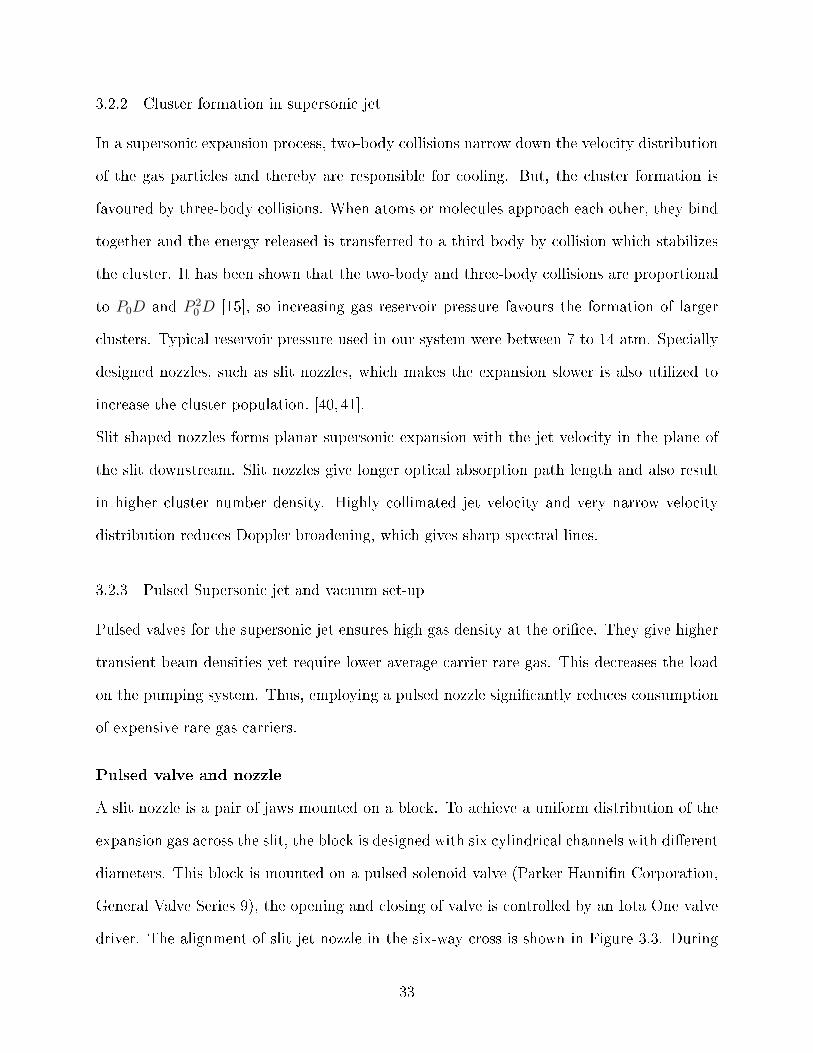
driver. The alignment of slit jet nozzle in the six-way cross is shown in Figure 3.3. During
33
this experiment methanol at -75oC was circulated around the slit nozzle using a cold copper
jacket and the circulating methanol was cooled by a Neslab Endocal Refrigerator. Cooling
of the nozzle was very crucial in observing benzene-noble gas trimers.
Figure 3.3: Pulsed slit nozzle and cold jacket con�guration inside the vacuum chamber.
Six-way cross vacuum chamber
The pulsed slit jet nozzle and the multipass cell are all inside a six-way cross vacuum chamber
(Figure 3.1). A 10" di�usion pump (Varian, VHS-10) backed by a mechanical pump (Ed-
wards, EM275) is used to evacuate the six-way cross. During the operation of the supersonic
jet the pressure inside the vacuum chamber is kept as low as 10−7 Torr.
3.3 Astigmatic Multi-pass Cell
The concentration of clusters in supersonic expansion is small (∼ 1013 clusters/cm3) and
when detecting a weak absorption band like a combination or an overtone band the change
in the laser intensity is small with respect to the initial laser intensity. So, the sensitivity
is limited by the laser �uctuations. In order to increase the sensitivity, a long absorption
pathlength is required, and since the expansion region is small this has to be done in a
limited space. One of the best ways is to use an astigmatic multipass cell. In an astigmatic
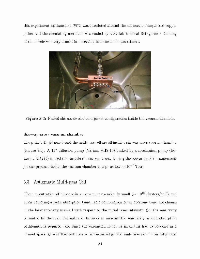
34
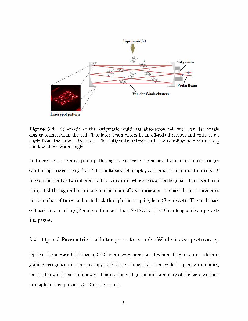
Figure 3.4: Schematic of the astigmatic multipass absorption cell with van der Waalscluster formation in the cell. The laser beam enters in an o�-axis direction and exits at anangle from the input direction. The astigmatic mirror with the coupling hole with CaF
2
window at Brewster angle.
multipass cell long absorption path lengths can easily be achieved and interference fringes
can be suppressed easily [43]. The multipass cell employs astigmatic or toroidal mirrors. A
toroidal mirror has two di�erent radii of curvature whose axes are orthogonal. The laser beam
is injected through a hole in one mirror in an o�-axis direction, the laser beam recirculates
for a number of times and exits back through the coupling hole (Figure 3.4). The multipass
cell used in our set-up (Aerodyne Research Inc., AMAC-100) is 70 cm long and can provide
182 passes.
3.4 Optical Parametric Oscillator probe for van der Waal cluster spectroscopy
Optical Parametric Oscillator (OPO) is a new generation of coherent light source which is
gaining recognition in spectroscopy. OPO's are known for their wide frequency tunability,
narrow linewidth and high power. This section will give a brief summary of the basic working
principle and employing OPO in the set-up.
35

3.4.1 Working principles of Optical Parametric Oscillators
An Optical Parametric Oscillator is very similar to a laser with a resonator design, but unlike
a laser, where the optical gain is from stimulated emission, in OPO the gain is obtained from
a process called parametric ampli�cation. Parametric ampli�cation involves the conversion
of a high intensity pump beam at frequency ωp to a lower frequencies signal (ωs) and idler
(ωi) in a nonlinear crystal with large second order non-linear susceptibility. This can be also
pictured as the pump photon converting into two lower energy photons, signal and idler,
satisfying the conservation of energy
ωp = ωs + ωi, (3.6)
and conservation of momentum,
kp = ks + ki. (3.7)
where k is the wavevector. The conservation of momentum is the phase matching condition
which determines the wavelength of the idler and the signal. When the phase matching con-
dition is satis�ed, amplitudes add up constructively from di�erent parts of the crystal and
thus high power conversion e�ciency is ensured. The most e�ective phase matching tech-
nique used by OPO's is quasi phase matching. In a crystal with high non-linear susceptibility
like LiNbO3this is done by �ipping the electric polarization of the crystal at the e�ective
interaction length of parametric generation or coherence length in a periodic fashion. This
is achieved by the application of an electric �eld and the process is called periodic poling.
The grating period determines the signal and idler wavelength.
The optical resonator or cavity in OPO provides feedback to the chosen frequency to
the gain medium, high re�ectivity mirrors are chosen for signal or idler frequency (singly
resonant OPO) or for both signal and idler (doubly resonant OPO). The OPO system we
are using (Lockheed Martin Argos Model 2400 - Module D) is a singly resonant OPO for
the idler as shown in Figure 3.5. The idler frequency region in this OPO covers a frequency
range from 3.9 to 4.6 µm (2173 to 2564 cm−1). The signal wavelength is between 1.3 to 1.4
36

µm and pump wavelength is at 1.064 µm. The nonlinear crystal in the OPO is a magnesium-
oxide doped periodically-poled lithium niobate (MgO:PPLN), with anti-re�ection coating for
signal, idler and pump wavelengths. MgO doping of PPLN increases the damage threshold.
The grating on the periodically poled lithium niobate (PPLN) crystal is fanned out (Figure
3.6), the idler frequency tuning is achieved by translation of crystal across the pump beam.
The translation changes the poling period that the pump beam is exposed to, which changes
the phase matching condition and consequently the wavelength. Figure 3.5 shows the crystal
using a single axis translational stage. The crystal is mounted in a temperature controlled
oven and it needs to be temperature stabilized between 45◦C and 70 ◦C with a precision
of 0.1◦ C. Coarse tuning of the wavelength is possible by changing the temperature, since
changing temperature changes the refractive index. The temperature stabilization of crystal
is time consuming, hence, crystal position tuning is preferred.
The OPO pump laser source is a diode pumped �ber optic laser with a power output
of 10 W at 1.064 µm. The seed laser for the 10 W �ber ampli�er is a distributed feedback
laser (DFB). The DFB laser source has a power of 10 mW and a linewidth of 100 KHz. The
piezoelectric transducer (PZT) strain of the �ber provides �ne tuning and scanning of the
pump laser frequency. A 0-100 V signal applied to the PZT element from PZT driver allows
a continuous idler frequency tuning over a 2 cm−1 range.
3.4.2 The experimental set-up with OPO source
Description of the set-up
Operation and data acquisition process
Each scan was acquired over a frequency window of 0.75-1 cm−1. This frequency window was
achieved by driving the PZT of the seed laser using a sine wave of 40 V amplitude and 100
Hz frequency. The sine wave was generated using a function generator. The data was taken
only on the rising part of the sine wave and near the zero crossing, where it is most linear.
37
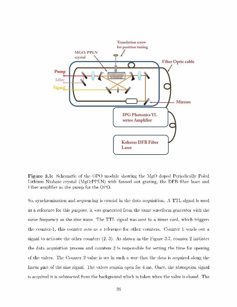
Figure 3.5: Schematic of the OPO module showing the MgO doped Periodically PoledLithium Niobate crystal (MgO:PPLN) with fanned out grating, the DFB �ber laser andFiber ampli�er as the pump for the OPO.
So, synchronization and sequencing is crucial in the data acquisition. A TTL signal is used
as a reference for this purpose, it was generated from the same waveform generator with the
same frequency as the sine wave. The TTL signal was sent to a timer card, which triggers
the counter-1, this counter acts as a reference for other counters. Counter 1 sends out a
signal to activate the other counters (2, 3). As shown in the Figure 3.7, counter 2 initiates
the data acquisition process and counters 3 is responsible for setting the time for opening
of the valves. The Counter 2 value is set in such a way that the data is acquired along the
linear part of the sine signal. The valves remain open for 4 ms. Once, the absorption signal
is acquired it is subtracted from the background which is taken when the valve is closed. The
38

Figure 3.6: Illustration of the OPO experimental set-up. Laser beams are shown with solidyellow lines, data signals with black lines, and synchronizing signals with dotted lines.
repetition rate of the scans is largely dependent on the time required by the di�usion pump
to exhaust the gas molecules from the six-way cross chamber, this may take 3 to 5 seconds.
Depending on the desired signal-to-noise ratio, each scan is averaged over 100 to 500 gas
pulses. The spectrum of a reference gas (N2O or CO
2) and etalon is acquired simultaneously
to calibrate the absorption spectrum of the van der Waals clusters in wavenumber scale. The
reference gas is kept in a glass cell with calcium �uoride window. The calcium �uoride has
a wavelength transmission of more than 90% from 0.1 to 8 µm.
39
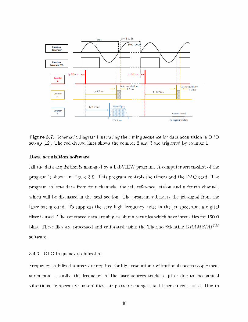
Figure 3.7: Schematic diagram illustrating the timing sequence for data acquisition in OPOset-up [12]. The red dotted lines shows the counter 2 and 3 are triggered by counter 1
Data acquisition software
All the data acquisition is managed by a LabVIEW program. A computer screen-shot of the
program is shown in Figure 3.8. This program controls the timers and the DAQ card. The
program collects data from four channels, the jet, reference, etalon and a fourth channel,
which will be discussed in the next section. The program subtracts the jet signal from the
laser background. To suppress the very high frequency noise in the jet spectrum, a digital
�lter is used. The generated data are single-column text �les which have intensities for 16000
bins. These �les are processed and calibrated using the Thermo Scienti�c GRAMS/AITM
software.
3.4.3 OPO frequency stabilization
Frequency stabilized sources are required for high resolution rovibrational spectroscopic mea-
surements. Usually, the frequency of the laser sources tends to jitter due to mechanical
vibrations, temperature instabilities, air pressure changes, and laser current noise. Due to
40
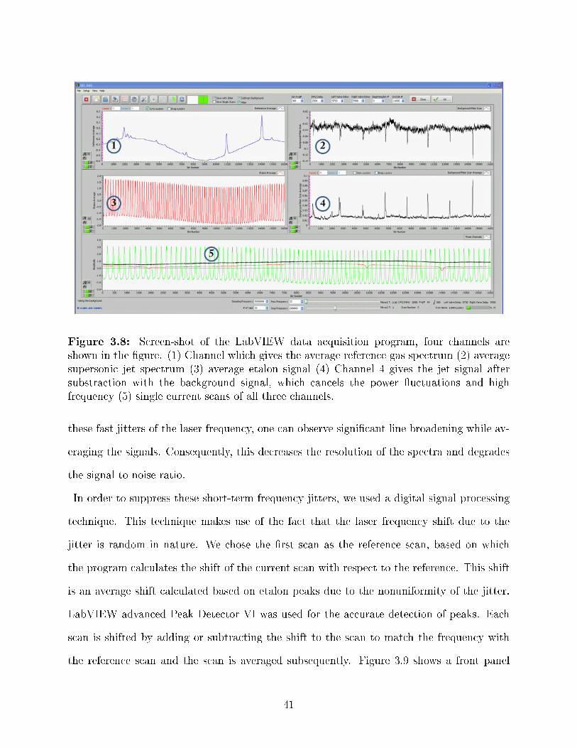
Figure 3.8: Screen-shot of the LabVIEW data acquisition program, four channels areshown in the �gure. (1) Channel which gives the average reference gas spectrum (2) averagesupersonic jet spectrum (3) average etalon signal (4) Channel 4 gives the jet signal aftersubstraction with the background signal, which cancels the power �uctuations and highfrequency (5) single current scans of all three channels.
these fast jitters of the laser frequency, one can observe signi�cant line broadening while av-
eraging the signals. Consequently, this decreases the resolution of the spectra and degrades
the signal to noise ratio.
In order to suppress these short-term frequency jitters, we used a digital signal processing
technique. This technique makes use of the fact that the laser frequency shift due to the
jitter is random in nature. We chose the �rst scan as the reference scan, based on which
the program calculates the shift of the current scan with respect to the reference. This shift
is an average shift calculated based on etalon peaks due to the nonuniformity of the jitter.
LabVIEW advanced Peak Detector VI was used for the accurate detection of peaks. Each
scan is shifted by adding or subtracting the shift to the scan to match the frequency with
the reference scan and the scan is averaged subsequently. Figure 3.9 shows a front panel
41

Figure 3.9: A screen-shot of the jitter suppression window, showing a portion of thereference etalon signal as blue trace and the current etalon signal as the black trace. Theshift of etalon peaks in each scan is calculated by the jitter suppression program relative tothe peaks of the reference signal peaks.
scree-shot of jitter suppression program.
3.4.4 SRO-OPO Power �uctuation suppression and background subtraction
For random noise reduction signal averaging is quite e�ective, since averaging increases the
signal strength by averaging out the noise. In the case of OPO, there are also �uctuations in
the spectra which are due to power �uctuations of the pump laser [39]. These �uctuations
are not random in nature, instead they add-up with signal averaging and obscures the weak
absorption lines. A previous study by W. Chen et al. [38] used a balanced detection tech-
nique, where the power �uctuation is removed by electronically subtracting the idler beam
from the signal beam. We implemented a similar set-up, where a reference beam separated
from the probe laser source is used instead of the idler beam. The power �uctuation is then
removed by electronically subtracting the reference beam from the absorption signal [12].
There is an extra channel for collecting the background signal was employed as shown in
Figure 3.6. The subtraction was done by using the LabVIEW program. Figure 3.10 shows
42

the screenshot demonstrating the implementation of the suppression of power �uctuations
in OPO.
Figure 3.10: The screen-shot of the computer screen, showing the e�ect of backgroundsubtraction on suppressing the power �uctuation. The black trace is before and the redtrace is after implementing the suppression technique.
43

Chapter 4
Infrared spectra of C6D6 −Rgn(n = 1,2)
4.1 Introduction
Weakly-bound rare gas (Rg) − benzene clusters provide attractive model systems for pro-
gressive solvation of an organic molecule, and their spectroscopy with rotational resolution
has an extensive history [11]. Thus, for example, electronic spectra have been obtained us-
ing laser induced �uorescence, coherent ion dip, or resonant enhanced two photon ionization
techniques for the complexes containing benzene together with He [14, 17], Ne [19], Ar [21]
- [23], Kr [24], and Xe [24], nonlinear Raman spectroscopy to He [25] and Ar [26], and mi-
crowave spectroscopy to Ne [27, 28], Ar [26, 29], Kr [30], and Xe [26]. Rg − benzene dimers
and trimers are found to have a simple structure in which the rare gas atom is on the average
located on the C6 symmetry axis at a distance of about r0 = 3.4 − 3.8 Å (depending on the
species) above and/or below the plane of the benzene molecule. The point group symmetry
of dimer reduces to C6v from D6h for the benzene monomer, and the point group of the
trimer remains the same as the monomer.
However, there have been no previous studies of Rg − benzene complexes in the infrared
region. This thesis reports such a study. This chapter discusses the analysis of the infrared
spectra of C6D
6− Rgn, (n=1,2) in the region of the ν12 C−D stretching band of C
6D
6near
2289 cm−1, where the rare gas (Rg) being He, Ne, or Ar. There have been very few previous
spectroscopic observations of He1,2− benzene. This work also represents the �rst observation
in any spectral region of the He1,2− and Ne1,2− C6D
6isotopologues.
C6D
6is chosen instead of C
6H
6because C
6H
6has no fundamental vibrations in our laser
region. The molecular structure of C6D
6and C
6H
6are the same, so the structures and in-
termolecular distance are similar. There is a strong Fermi (anharmonic) resonance between
44
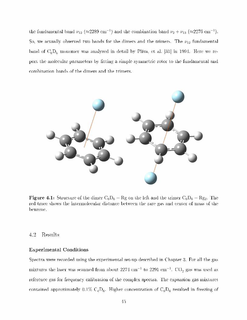
the fundamental band ν12 (≈2289 cm−1) and the combination band ν2 + ν13 (≈2276 cm−1).
So, we actually observed two bands for the dimers and the trimers. The ν12 fundamental
band of C6D
6monomer was analyzed in detail by Plíva, et al. [31] in 1994. Here we re-
port the molecular parameters by �tting a simple symmetric rotor to the fundamental and
combination bands of the dimers and the trimers.
Figure 4.1: Structure of the dimer C6D6 − Rg on the left and the trimer C6D6 − Rg2. Thered trace shows the intermolecular distance between the rare gas and center of mass of thebenzene.
4.2 Results
Experimental Conditions
Spectra were recorded using the experimental set-up described in Chapter 3. For all the gas
mixtures the laser was scanned from about 2274 cm−1 to 2291 cm−1. CO2gas was used as
reference gas for frequency calibration of the complex spectra. The expansion gas mixtures
contained approximately 0.1% C6D
6. Higher concentration of C
6D
6resulted in freezing of
45
the nozzle. The carrier gas was He for C6D6 − He1,2, a 1:2 mixture of Ne:He for C6D6 − Ne1,2,
and a 1:5 mixture of Ar:He for C6D6 − Ar1,2. The ratios of the gas mixture was optimized to
obtain the maximum concentration of complexes in the jet. The backing pressure of the gas
sample in the reservoir were about 9 atm, this was increased to 13 atm for the observation
of trimer.
Simulation and �tting of data
The objective is to determine the molecular parameters for the ground and excited state
mentioned in the rotational energy as given by Equation 2.51. The PGOPHER computer
program [35] was used for spectral simulation which is a general purpose program for simulat-
ing and �tting rotational, vibrational and electronic spectra with a graphical user interface.
In order to begin with the simulation, the easiest way is to guess the structure of the vdW
complex. I considered the symmetric top structures for the dimers and trimers as shown in
Figure 4.1 These structures were considered from some of previously determined structures
using microwave and electronic spectra [11].
The rotational constants of the assumed structure were derived using a program that de-
termines the principal moments of inertia of the molecules (PMIFST) [44]. These rotational
constants were used to create a simulation for an initial comparison with the observed spec-
tra. Some of the parameters need to be �xed before assigning the transitions frequencies: the
rotational temperature, the line shape, point group symmetry of the complex, nuclear statis-
tical weights (Section 2.6.1) and the symmetry element of the ground and excited vibrational
state.
As discussed in Section 2.4, the rotational constant of a symmetric top around the sym-
metry axis (A or C) cannot be easily determined from parallel bands. The position of rare gas
atoms for the dimers and the trimers, as shown in Figure 4.1, does not change the moment of
inertia about the C6 symmetry axis. Hence, the parameter A or C for the ground vibrational
state of C6D6 − Rg1,2 complexes were �xed at the C6D
6monomer C value, 0.078496 cm−1,
46

determined previously by Plíva et al. [30,36]. It should be noted that C6D
6-He1,2 complexes
are oblate symmetric tops, C6D
6-Ne1,2 and C
6D
6-Ar1,2 are prolate symmetric tops (Section
2.3.1).
For a symmetric top, the spectral pattern follow the selection rules for parallel or per-
pendicular band, as described in Section 2.6 (Equations 2.69 and 2.70). Since, the observed
band is C-D stretch (ν12) and ring stretch (ν2 + ν13) vibrational mode, the change in dipole
moment is perpendicular to the symmetric top axis of the benzene. Hence, the observed
band is perpendicular. Each observed line is a transition between the rotational quantum
numbers J and K, with the selection rules one can determine the allowed transitions. Lower
K lines are assigned �rst, the low J lines are usually located near the band center. Each J
value, the corresponding K lines are assigned by varying a minimum number of parameters.
Eventually, 15 parameters were varied and determined from the simulation for the dimers.
The ground state molecular parameters were rotational constant B" and centrifugal distor-
tion constants DJK" and DJ". The excited state parameters determined for the fundamental
and combination band are vibrational band origins ν0, rotational constants B′, C ′ or A′, the
centrifugal distortion constants D′JK , D
′J and the coriolis coupling constant ζ
′. Similarly,
11 parameters were determined for trimers. Distortion constants were not determined for
trimers due to fewer number of observed lines and the fact that these are heavier species.
The spectra were �tted to symmetric top structures as shown in the Figure 4.1. The
assumed Gaussian line width was 0.002 cm−1 (60 MHz). The simulated spectra used an
e�ective rotational temperature of 2.5 K for the dimers and 1.5 K for the trimers. Nuclear
spin weights for the point group symmetry of C6v and D6h are given in Table 4.1.
4.2.1 He1,2 − C6D6
Three previous publications on the C6D6 − He1,2 complex are especially relevant here. The
�rst, from 1979, is a pioneering laser induced �uorescence study of the electronic spectrum
by Beck et al. [14], who studied the S1 ← S0 610 (ν61← 0) vibronic band (≈38610 cm−1) in
47

a pulsed supersonic jet expansion with an e�ective rotational temperature of about 0.3 K.
The spectrum was remarkably clear and clean, but the accuracy of their �tted parameters
was limited by their spectral resolution (≈0.04 cm−1). Recently, the same spectrum was re-
examined by Hayashi and Ohshima [17] under similar conditions, but with greatly improved
resolution (<0.01 cm−1) using resonant enhanced two photon ionization spectroscopy. Their
analysis yields a value of r0 ≈ 3.60 Å for the e�ective distance between the He atom and the
benzene plane for the dimer and trimer. The third key paper, by Lee et al. [25], describes
nonlinear Raman spectroscopy results, together with an analytical potential energy surface
for He−C6H
6which is based on high-level ab initio calculations. This potential surface yields
a very similar value for r0 (3.61Å), and also gives a value of re = 3.16 Å for the equilibrium
intermolecular separation, that is, the global minimum of the surface itself, at an energy of
-89.6 cm−1.
We observed C6D
6−He and C
6D
6−He
2spectra accompanying both the ν12 and ν2 + ν13
bands, as illustrated in Figure 4.2. The stronger lines were assigned to the C6D
6monomer, as
described in Ref. [31], these strong C6D
6lines were removed from the Figure 4.2 for an e�ec-
tive comparison between the observed and simulated spectra of C6D
6−He and C
6D
6−He
2.
The dimer bands are roughly 6 times weaker than the monomer bands and trimer bands
are 12 times weaker. The ground state rotational constant C is �xed as the monomer for
all the complexes. We assigned and �tted 90 spectral lines in terms of 140 transitions for
dimer and 60 spectral lines were assigned for 69 transitions for trimer, and varying a total of
16 parameters. This was a simultaneous �t, so that both observed band, fundamental and
combination band helped to determine the ground state parameters.
The resulting molecular parameters for the C6D
6−He dimer are given in Table 4.2. Note
that it was possible to determine a value for the l-type doubling parameter q (see Section
2.5) for the ν2 + ν13 upper state (2275.96 cm−1 band) for C6D
6−He, but not for the ν12
fundamental (nor for any of the He2−, Ne1,2− or Ar1,2− C
6D
6bands below). The simulated
48

Figure 4.2: Observed (black trace) fundamental ν12 band (top) and ν2+ν13 bands (bottom).The simulated (blue and red trace) spectra of C
6D
6−He dimer is shown in blue trace and
C6D
6−He
2trimer in red trace.
49

spectra are based on these parameters and assume a temperature of 2.5 K for the dimers and
1.5 K for the trimers with line widths of 0.0029 cm−1 and 0.002 cm−1, respectively (Figure
4.2). They are calculated using the parameters from Table 4.2. For simulating the intensity,
we also included nuclear spin statistical weights of rovibrational levels (Section 2.6.1), which
are given in Table 4.1.
Table 4.1: Nuclear spin weights of respective symmetries for C6v (dimer) and D6h (trimer)
C6v A1,A2 B1,B2 E1 E2
130 119 232 248
D6h A1g,A1u A2g,A2u B1g,B1u B2g,B2u E1g,E1u E2g,E2u
74 56 55 64 116 124
The molecular parameters for C6D
6−He
2are given in Table 4.3. The centrifugal distor-
tion constants (see Section 2.4) for the trimers were not determined because of fewer number
of assigned lines.
4.2.2 Ne1,2 − C6D6
The C6H
6−Ne dimer has been studied by electronic [17] and microwave [26,27] spectroscopy,
but there are no previous reports of dimer C6D
6−Ne or trimer C
6D
6−Ne
2in the IR region.
The dimer and trimer spectra are shown in Figure 4.3. A total of 63 lines were �tted in
terms of 199 transitions in a simultaneous analysis to give the C6D
6−Ne parameters listed
in Table 4.2. For trimer C6D
6−Ne
2, 46 lines were assigned in terms of 67 transitions given in
Table 4.3. The ground state constant for rotation around the symmetric top axis (this is now
labelled A) was again �xed at the monomer C-value. We noted that the microwave values
of the distortion constants DJK and DJ are quite similar for C6H
6−Ar and C
6D
6−Ar [28],
therefore estimated values of these constants for C6D
6−Ne by simple scaling of those of
C6H
6−Ne [26] according to their ratios for the Ar complexes. These scaled values were held
50
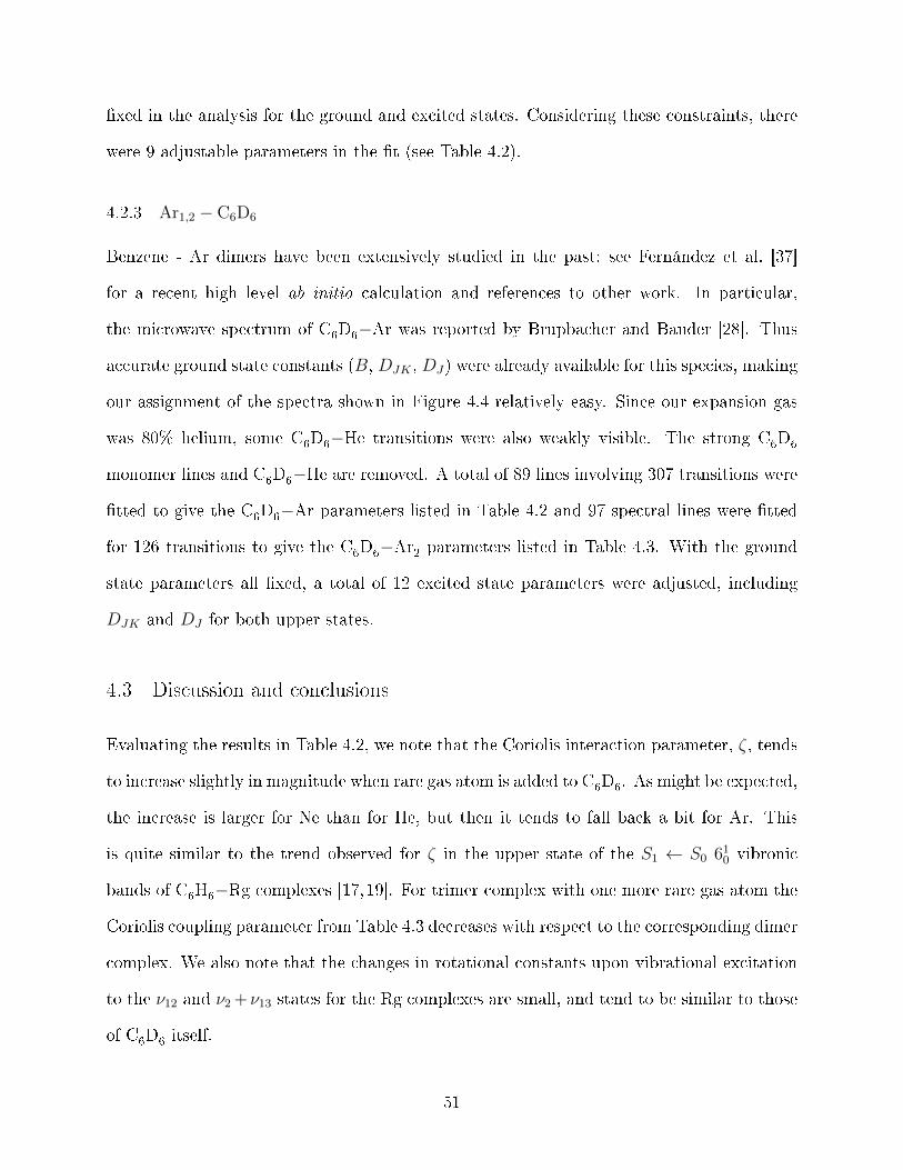
�xed in the analysis for the ground and excited states. Considering these constraints, there
were 9 adjustable parameters in the �t (see Table 4.2).
4.2.3 Ar1,2 − C6D6
Benzene - Ar dimers have been extensively studied in the past; see Fernández et al. [37]
for a recent high level ab initio calculation and references to other work. In particular,
the microwave spectrum of C6D
6−Ar was reported by Brupbacher and Bauder [28]. Thus
accurate ground state constants (B, DJK , DJ) were already available for this species, making
our assignment of the spectra shown in Figure 4.4 relatively easy. Since our expansion gas
was 80% helium, some C6D
6−He transitions were also weakly visible. The strong C
6D
6
monomer lines and C6D
6−He are removed. A total of 89 lines involving 307 transitions were
�tted to give the C6D
6−Ar parameters listed in Table 4.2 and 97 spectral lines were �tted
for 126 transitions to give the C6D
6−Ar
2parameters listed in Table 4.3. With the ground
state parameters all �xed, a total of 12 excited state parameters were adjusted, including
DJK and DJ for both upper states.
4.3 Discussion and conclusions
Evaluating the results in Table 4.2, we note that the Coriolis interaction parameter, ζ, tends
to increase slightly in magnitude when rare gas atom is added to C6D
6. As might be expected,
the increase is larger for Ne than for He, but then it tends to fall back a bit for Ar. This
is quite similar to the trend observed for ζ in the upper state of the S1 ← S0 610 vibronic
bands of C6H
6−Rg complexes [17,19]. For trimer complex with one more rare gas atom the
Coriolis coupling parameter from Table 4.3 decreases with respect to the corresponding dimer
complex. We also note that the changes in rotational constants upon vibrational excitation
to the ν12 and ν2 + ν13 states for the Rg complexes are small, and tend to be similar to those
of C6D
6itself.
51

Figure 4.3: Observed (black trace) fundamental ν12 band (top) and ν2+ν13 bands (bottom).The simulated (blue and red trace) spectra of C
6D
6−Ne dimer is shown in blue trace and
C6D
6−Ne
2trimer in red trace.
52
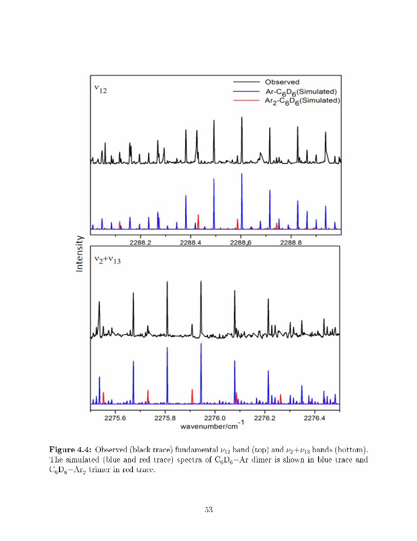
Figure 4.4: Observed (black trace) fundamental ν12 band (top) and ν2+ν13 bands (bottom).The simulated (blue and red trace) spectra of C
6D
6−Ar dimer is shown in blue trace and
C6D
6−Ar
2trimer in red trace.
53

Table 4.2: Molecular parameters for the C6D
6
a and C6D
6− Rg complex (in cm−1). Un-
certainties in parenthesis are 1σ from the least-squares �ts in units of the last quoted digit.
C6D6 [31, 36]b C6D6 − He C6D6 − Ne C6D6 − ArGround stateB" 0.15701902 0.107559(23) 0.056149(17) 0.03710704C"(A")c 0.078496 0.078496 0.078496 0.078496DJK"×10−7 -0.4174 14.7(69) 24d 4.847DJ"×10−7 0.25 0.01(51) 5.3d 0.892Excited state combination bandν0 2275.8776(1) 2275.9621(2)e 2275.9206(2) 2275.8498(1)B′
0.1567464(68) 0.107577(22) 0.056147(17) 0.0370964(28)C′/A′
0.0783580(50) 0.078350(18) 0.078386(18) 0.0783220(78)ζ′
-0.33501 -0.34140(39) -0.34482(36) -0.33816(11)D′JK × 10−7 -0.4174 -28.3(55) 24 5.45(86)
D′J × 10−7 0.25 37.7(44) 5.3 0.33(20)
Excited state fundamental bandν0 2288.7395(2) 2288.7326(2) 2288.6725(2) 2288.5337(1)B′
0.1568001(48) 0.107632(31) 0.056143(17) 0.0371050(23)C′/A′
0.0784018(37) 0.078401(26) 0.078395(16) 0.0784608(76)ζ′
-0.17017 -0.18180(33) -0.18621(29) -0.18347(10)D′JK × 10−7 -0.4174 -47.9(91) 24 4.25(65)
D′J × 10−7 0.25 49.8(76) 5.3 0.5(15)
a Units of cm−1, except for ζ which is dimensionless. Uncertainties in parentheses are 1σexpressed in units of the last quoted digit; parameters without uncertainties were �xed.b DK = 1.88× 10⁻⁸ cm−1 for all C
6D
6states.
c Parameter for rotation about the C6 symmetry axis, assumed in the ground state to beequal to that of C
6D
6. This is labelled C for C
6D
6and C
6D
6−He, or A for C
6D
6−Ne and
−Ar.d Scaled from known [27] C
6H
6−Ne parameters by the ratio for C
6D
6−Ar and C
6H
6−Ar.
e Also: q = −9.2(20) × 10−5 (l-type doubling parameter) for the 2275.9621 cm�1 state ofC6D
6−He.
A key result from the deuterated benzene − Rg1,2 spectrum is the B-value, which directly
gives the intermolecular separation with the assumption that the monomer structure remains
unchanged in the dimer and trimer. A structure �tting program (STRFIT) [44] was used
to calculate the intermolecular separation. This is obtained by assuming the monomer
(benzene) structure and varying the distance between the benzene plane and the rare gas
atom for the corresponding B-value. Experimental results for the intermolecular distances
between He, Ne, or Ar and C6H
6or C
6D
6for the dimer and trimer are summarized in Table
4.4. Table 4.4 thus con�rms that our new B-values for C6D
6− Rg1,2 are entirely consistent
54
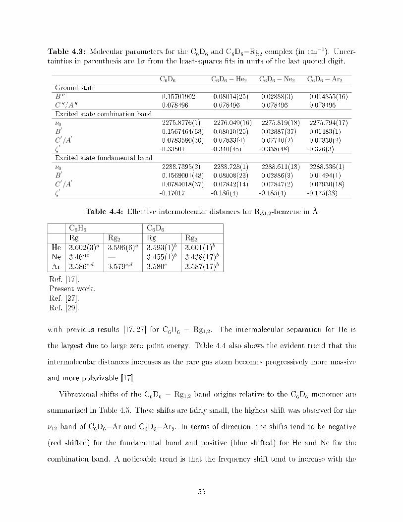
Table 4.3: Molecular parameters for the C6D
6and C
6D
6−Rg
2complex (in cm−1). Uncer-
tainties in parenthesis are 1σ from the least-squares �ts in units of the last quoted digit.
C6D6 C6D6 − He2 C6D6 − Ne2 C6D6 − Ar2
Ground stateB" 0.15701902 0.08014(25) 0.02888(3) 0.014855(16)C"/A" 0.078496 0.078496 0.078496 0.078496Excited state combination bandν0 2275.8776(1) 2276.049(16) 2275.819(18) 2275.794(17)B′
0.1567464(68) 0.08010(25) 0.02887(37) 0.01483(1)C′/A′
0.0783580(50) 0.07833(4) 0.07710(2) 0.07830(2)ζ′
-0.33501 -0.340(45) -0.338(48) -0.326(3)Excited state fundamental bandν0 2288.7395(2) 2288.728(1) 2288.611(18) 2288.336(1)B′
0.1568001(48) 0.08008(23) 0.02886(3) 0.01494(1)C′/A′
0.0784018(37) 0.07842(14) 0.07847(2) 0.07930(18)ζ′
-0.17017 -0.186(4) -0.185(4) -0.175(38)
Table 4.4: E�ective intermolecular distances for Rg1,2-benzene in Å
C6H6 C6D6
Rg Rg2 Rg Rg2
He 3.602(3)a 3.596(6)a 3.593(1)b 3.601(1)b
Ne 3.462c � 3.455(1)b 3.438(17)b
Ar 3.586c,d 3.579c,d 3.580c 3.587(17)b
Ref. [17].Present work.Ref. [27].Ref. [29].
with previous results [17, 27] for C6H
6− Rg1,2. The intermolecular separation for He is
the largest due to large zero point energy. Table 4.4 also shows the evident trend that the
intermolecular distances increases as the rare gas atom becomes progressively more massive
and more polarizable [17].
Vibrational shifts of the C6D
6− Rg1,2 band origins relative to the C
6D
6monomer are
summarized in Table 4.5. These shifts are fairly small, the highest shift was observed for the
ν12 band of C6D
6−Ar and C
6D
6−Ar
2. In terms of direction, the shifts tend to be negative
(red shifted) for the fundamental band and positive (blue shifted) for He and Ne for the
combination band. A noticeable trend is that the frequency shift tend to increase with the
55

Table 4.5: Vibrational shift relative to C6D6 vibration in cm-1
shift ν12 shift ν2 + ν13 ν12 minus ν2 + ν13
C6D6 0.0 0.0 12.862C6D6 − He −0.0069 +0.0845 12.771C6D6 − Ne −0.0668 +0.0430 12.752C6D6 − Ar −0.2058 −0.0278 12.684C6D6 − He2 −0.012 +0.084 12.68C6D6 − Ne2 −0.206 −0.028 12.79C6D6 − Ar2 −0.404 −0.084 12.54
addition of rare gas atoms. The last column of Table 4.5 shows that there is a small decrease
in the separation between the ν12 and ν2 +ν13 band origins in going from the C6D
6monomer
to the dimer and trimer. This could be indicating that, as the rare gas mass increases, there
is a decrease in the magnitude of the Fermi interaction coupling these vibrations. On the
other hand, it could be interpreted as simply being due to di�ering vibrational shift e�ects
for the two vibrational modes.
56
Chapter 5
Conclusions
Rare gas - benzene van der Waals molecules were among the �rst weakly bound complexes
investigated by laser spectroscopy in a supersonic jet. Since 1979 [14], the interest in such
species has continued to the present time, the main reason being the simplicity of the in-
termolecular forces among these species. Thus, the quantitative comparison between the
experiment and ab initio calculation of clusters is considered feasible. The infrared study of
complexes leads to detailed information regarding the vibrationally averaged structure. The
formation of structure is governed by the intermolecular forces. Information pertaining to
these intermolecular interactions is contained in the experimental results.
The experimental results were obtained using the set-up described in chapter 3. The
thesis discussed the improvement implemented on the experimental set-up. The implemen-
tation of OPO as the probe laser and increasing of the signal to noise ratio by suppressing
the power �uctuations of the OPO laser. Also, the cooling of the supersonic-jet nozzle by
circulating with methanol at −75oC was implemented for the present work, which enabled
the observation of the benzene - rare gas trimer complexes that is discussed.
This thesis presents an investigation on deuterated benzene - rare gas (Rg) dimer and
trimer complexes using high resolution infrared spectroscopy. The rare gas used were He,
Ne and Ar. The thesis reports the �rst study and observation of benzene − Rg1,2 complexes
in the infrared region and also reports the �rst observation of C6D
6− Ne
2in any spectral
region. A strong Fermi resonance between the fundamental band ν12 and the combination
band ν2 + ν13 were observed for each dimer and trimer. The present work on C6D6 − Rg1,2
complexes were observed with an e�ective rotational temperature of about 2.5 K for the
dimers and 1.5 for the trimers. The spectra were observed with a resolution of ∼ 60 MHz
57

which is the highest observed for benzene - rare gas complexes. The results presented for
the dimers were published in Chemical Physics Letters [46].
The rotational parameters were determined by simulating the observed spectra. The
structure of the complexes and the intermolecular distances were derived from the rotational
parameters. The C6D
6− Rg1,2 dimers and trimers are found to have a simple structure
in which the rare gas atom is located on the C6 symmetry axis of the benzene monomer.
Depending on the species the rare gas atom is found to be located at a distance of 3.4 − 3.8
Å from the plane of the benzene molecule. For the trimer the rare gas atoms are localized
on the C6 symmetry axis, symmetrically on the opposite sides of the benzene plane. The
dimer formation reduces the point group symmetry from D6h symmetry for the benzene
monomer to C6v and the trimer symmetry is same as the monomer. The results provided a
benchmark for re�ning the potential energy surfaces which describe the intermolecular forces
acting between the monomers.
In the future, higher complexes (tetramer, pentamer etc.) can be observed with benzene
being soluted by noble gas atoms. The behaviour of Fermi resonance phenomena with the
formation of larger complexes need to be further investigated. The high-resolution measure-
ments can also be extended to larger planar aromatic molecules. To observe higher complexes
it is required to rotationally cool the molecules to less than 1 K. For the present set-up this
might be possible by further cooling the gas before the cluster formation, U. Evan et al. [42]
achieved this by implementing a specially designed high pressure valve with miniaturized
valve parts.
The benzene - rare gas trimer observed in this study was 12 times weaker than the
monomer (benzene) spectral lines. The line strength decreases with the size of the complexes.
To observe weaker lines the sensitivity of the system must be improved. One way is to increase
the path length of the multipass absorption cell. The multipass cell used in our spectrometer
(Aerodyne Research Inc., AMAC-100) is aligned to provide 182 laser passes. McManus [43]
58
showed that by changing the separation between the mirrors and rotation about the optical
axis, the number of passes can be increased to 274 or 366. This will increase the e�ective
absorption path length in the system and should provide higher signal to noise ratio.
The resolution of the obtained spectra from the current set-up was ∼ 60 MHz. To observe
the larger complexes it is required to improve the resolution. As the size of the complexes,
the band origin of the complexes tend to shift with respect to the monomer band origin,
as shown in Table 4.5, this shift is very small and one needs to increase the resolution of
the system to observe this shift. The laser line width of the OPO is less than 1 MHz, so
it is possible to further increase the resolution. The residual Doppler broadening can be
decreased by implementing a skimmer [45].
59
Bibliography
[1] P. R. Bunker and P. Jensen, Molecular Symmetry and Spectroscopy, NRC Research
Press, Ottawa, 2nd edition (1998).
[2] D. Papou²ek and M. R. Aliev, Molecular Vibrational-Rotational Spectra, Elsevier Sci-
enti�c Publishing Co., Amsterdam/Oxford/New York, (1982).
[3] P. R. Bunker and P. Jensen, Fundamentals of Molecular Symmetry, Institute of Physics
Publishing, Bristol/Philadelphia, (2005).
[4] H. C. Allen and P. C. Cross, Molecular Vib-Rotors, Elsevier Scienti�c Publishing Co.,
New York and London, (1963).
[5] W. Demtröder, Molecular Physics - Theoretical Principles and Experimental Methodes,
WILEY-VCH, (2003).
[6] R. N. Zare, Angular Momentum: Understanding Spatial Aspects in Chemistry and
Physics, Wiley, New York (1988).
[7] W. Gordy and R. L. Cook, Microwave Molecular Spectra, Wiley, (1984).
[8] D. J. Willock, Molecular Symmetry, Wiley, (2009).
[9] B. K. Shivamoggi, Theoretical Fluid Mechanics, Wiley, (1998).
[10] M. V. Johnston, Trends Anal. Chem., vol. 3, no.2 (1984).
[11] H. J. Neusser, R. Sussman, Jet Spectroscopy and Molecular Dynamics, eds. J. M.
Hollas, D. Phillips, Springer Media, New York (1995) 118.
[12] M. Rezaei, High-Resolution Pulsed Slit Jet Spectrometer with QCL and OPO probes for
Infrared Spectroscopy on van der Waals Clusters, PhD Thesis, University of Calgary
(2014).
60

[13] J. N. Oliaee, High Resolution Infrared Spectroscopy of van der Waals Clusters of Nitrous
Oxide, Carbon Dioxide and OCS-R Complexes, PhD Thesis, University of Calgary
(2013).
[14] S. M. Beck, M. G. Liverman, D. L. Monts, R. E. Smalley, J. Chem. Phys. 70, 232
(1979).
[15] R. E. Smalley, L. Wharton and D. H. Levy, Acc. Chem. Res. 10, 139 (1977).
[16] J. Koperski and E. S. Fry, J. Phys. B: At. Mol. Opt. Phys. 39, 1125 (2006).
[17] M. Hayashi, Y. Ohshima, Chem. Phys. 419, 131 (2013).
[18] D. M. Lubman, C. Retiner and R. N. Zare, J. Phys. Chem. 86, 1129 (1982).
[19] T. Weber, E. Riedle, H. J. Neusser, E. W. Schlag, J. Mol. Structure 249, 69 (1991).
[20] H. J. Neusser, R. Sussman, A. M. Smith, E. Riedle, T. Weber, Ber. Bunsenges. Phys.
Chem. 96, 1252 (1992).
[21] T. Weber, A. Von Bargen, E. Riedle, H. J. Neusser, J. Chem. Phys. 92, 90 (1990).
[22] R. Sussmann, R. Neuhauser, H. J. Neusser, J. Chem. Phys. 103, 3315 (1995).
[23] R. Neuhauser, J. Braun, H. J. Neusser, A. van der Avoird, J. Chem. Phys. 108, 8408
(1998) .
[24] T. Weber, E. Riedle, H. J. Neusser, E. W. Schlag, Chem. Phys. Lett. 183, 77 (1991).
[25] S. Lee, J.S. Chung, P. M. Felker, J. L. Cacheiro, B. Fernández, T. B. Pedersen, H.
Koch, J. Chem. Phys. 119, 12956 (2003).
[26] W. Kim, P. M. Felker, J. Chem. Phys. 107, 2193 (1997).
[27] E. Arunan, T. Emilsson, H.S. Gutowksy, J. Chem. Phys. 101, 861 (1994).
61

[28] T. Brupbacher, J. Makarewicz, A. Bauder, J. Chem. Phys. 101, 9736 (1994).
[29] T. Brupbacher, A. Bauder, Chem. Phys. Lett. 173, 435 (1990).
[30] T. D. Klots, T. Emilsson, H. S. Gutowsky, J. Chem. Phys. 97, 5335 (1992).
[31] J. Plíva, J.W.C. Johns, L. Goodman, J. Mol. Spectrosc. 163, 108 (1994).
[32] M. Rezaei, A.R.W. McKellar, N. Moazzen-Ahmadi, J. Mol. Spectrosc. 296 (2014) 14.
[33] M. Dehghani, M. Afshari, Z. Abusara, N. Moazzen-Ahmadi, A.R.W. McKellar, J.
Chem. Phys. 126, 164310 (2007).
[34] N. Moazzen-Ahmadi, A.R.W. McKellar, Int. Rev. Phys. Chem. 32, 611 (2013).
[35] C. M. Western, a program for simulating rotational structure PGOPHER, University
of Bristol, UK; See http://pgopher.chm.bris.ac.uk.
[36] J. Plíva, A. Valentin, J. Chazelas, L. Henry, J. Mol. Spectrosc. 134 220 (1989).
[37] S. B. Capelo, B. Fernández, H. Koch, P. M. Felker, J. Phys. Chem. A 113, 5212 (2009).
[38] W. Chen, G. Mouret, D. Boucher, Appl. Phys. B 67, 375 (1998).
[39] M Vainio, M. Siltanen, J. Peltola, L. Halonen, Appl. Opt. 50, 4 (2010).
[40] O. F. Hagena, and W. Obert, J. Chem. Phys. 56, 1793 (1972).
[41] J. B. Hopkins, P.R. Langridge-Smith, M. D. Morse, and R. E. Smalley, J. Chem. Phys.
78, 1627 (1983).
[42] U. Evan, J. Jortner, D. Noy, N. Lavie, and C. Cossart-MagosChem, J. Chem. Phys.
112, 8068 (2000).
[43] J. B. McManus, P. L. Kebabian, and M. S. Zahniser, Appl. Opt. 34, 3336 (1995).
62

[44] Z. Kisiel, http://www.ifpan.edu.pl/ kisiel/struct/struct.htm
[45] R. Campargue, Rev. Sci. Instrum. 35 , 111 (1964).
[46] J. George, A. R. W McKellar, and N. Moazzen-Ahmadi, Chem. Phys. Lett. 610, 121
(2014).
63

Appendix A
Supplementary data for Chapter 4
Dimer Complexes
Calculated and observed transitions for C6D
6−He, C
6D
6−Ne and C
6D
6−Ar dimers.
Table A.1: Observed transitions in the ν2 + ν13 (∼ 2275 cm−1) and ν12 (∼ 2288 cm−1)
bands of C6D
6−He (values in cm−1).
J ′ K ′ L′ J ′′ K ′′ Observed Calculated Obs.-Calc.6 6 -1 7 7 2274.5093 2274.5094 -0.00015 3 -1 6 4 2274.7128 2274.7118 0.00105 4 -1 6 5 2274.7170 2274.7163 0.00075 5 -1 6 6 2274.7206 2274.7209 -0.00035 5 -1 6 6 2274.7206 2274.7209 -0.00034 1 -1 5 2 2274.9189 2274.9192 -0.00034 2 -1 5 3 2274.9242 2274.9237 0.00054 2 -1 5 3 2274.9242 2274.9237 0.00054 3 -1 5 4 2274.9281 2274.9280 0.00014 4 -1 5 5 2274.9322 2274.9323 0.00003 0 4 1 2275.1297 2275.1305 -0.00083 1 -1 4 2 2275.1344 2275.1350 -0.00073 2 -1 4 3 2275.1397 2275.1394 0.00033 2 -1 4 3 2275.1397 2275.1394 0.00033 3 -1 4 4 2275.1432 2275.1435 -0.00032 1 1 3 0 2275.3411 2275.3413 -0.00022 0 3 1 2275.3455 2275.3458 -0.00042 1 -1 3 2 2275.3503 2275.3504 -0.00012 2 -1 3 3 2275.3548 2275.3546 0.00022 2 -1 3 3 2275.3548 2275.3546 0.00021 0 2 1 2275.5612 2275.5610 0.00021 1 -1 2 2 2275.5658 2275.5655 0.00030 0 1 1 2275.7765 2275.7761 0.00055 4 1 5 3 2275.9699 2275.9689 0.00107 2 1 7 1 2275.9699 2275.9706 -0.0007
64

J ′ K ′ L′ J ′′ K ′′ Observed Calculated Obs.-Calc.4 4 1 4 3 2275.9699 2275.9700 -0.00015 4 1 5 3 2275.9699 2275.9689 0.00106 3 1 6 2 2275.9699 2275.9711 -0.00124 4 1 4 3 2275.9699 2275.9700 -0.00014 3 1 4 2 2275.9752 2275.9753 -0.00016 2 1 6 1 2275.9752 2275.9756 -0.00043 3 1 3 2 2275.9752 2275.9759 -0.00072 2 1 2 1 2275.9807 2275.9813 -0.00064 2 1 4 1 2275.9807 2275.9803 0.00043 2 1 3 1 2275.9807 2275.9811 -0.00044 1 1 4 0 2275.9857 2275.9844 0.00131 1 1 1 0 2275.9857 2275.9863 -0.00062 1 1 2 0 2275.9857 2275.9861 -0.00043 1 1 3 0 2275.9857 2275.9856 0.00021 0 1 1 2275.9911 2275.9912 -0.00013 0 3 1 2275.9911 2275.9909 0.00022 0 2 1 2275.9911 2275.9912 -0.00014 0 4 1 2275.9911 2275.9902 0.00093 1 -1 3 2 2275.9951 2275.9954 -0.00032 1 -1 2 2 2275.9951 2275.9957 -0.00054 1 -1 4 2 2275.9951 2275.9947 0.00046 3 -1 6 4 2275.9991 2275.9998 -0.00074 2 -1 4 3 2275.9991 2275.9991 0.00004 2 -1 4 3 2275.9991 2275.9991 0.00003 2 -1 3 3 2275.9991 2275.9997 -0.00073 2 -1 3 3 2275.9991 2275.9997 -0.00071 1 1 0 0 2276.2020 2276.2016 0.00032 2 1 1 1 2276.4119 2276.4116 0.00032 1 1 1 0 2276.4171 2276.4169 0.00022 0 1 1 2276.4216 2276.4214 0.00013 3 1 2 2 2276.6218 2276.6212 0.00073 2 1 2 1 2276.6267 2276.6264 0.00023 1 1 2 0 2276.6319 2276.6320 -0.00023 0 2 1 2276.6365 2276.6363 0.00024 4 1 3 3 2276.8309 2276.8304 0.00054 4 1 3 3 2276.8309 2276.8304 0.0005
65
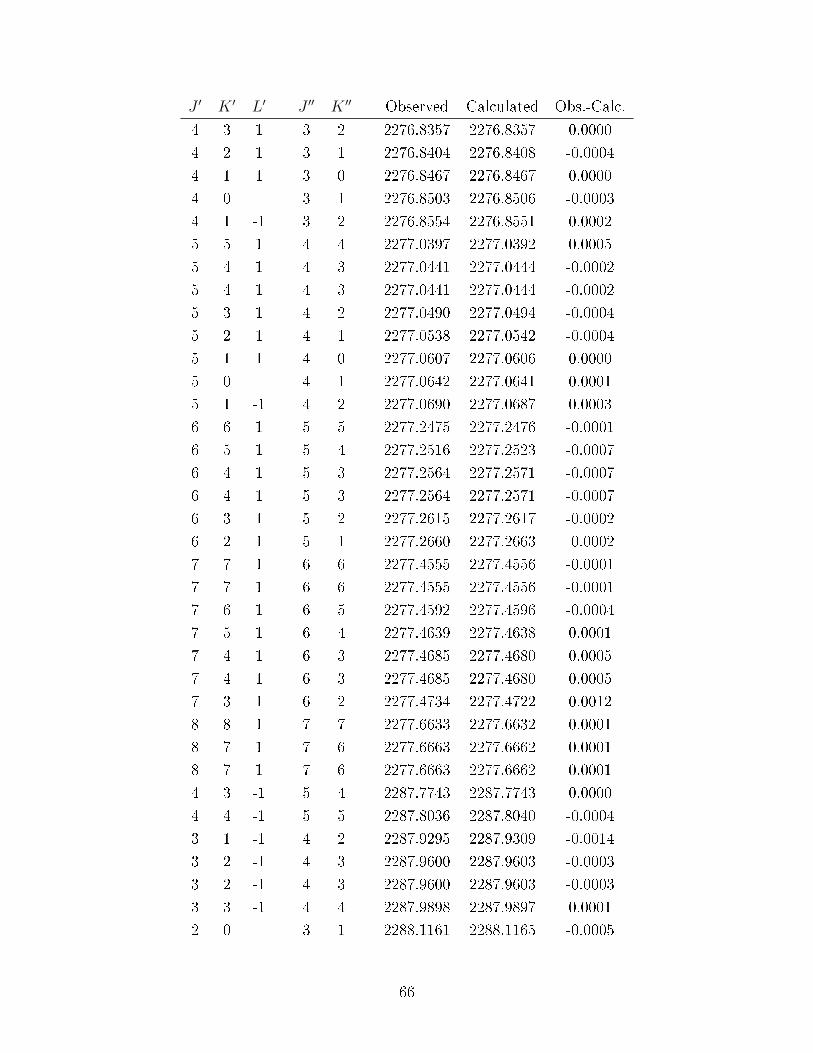
J ′ K ′ L′ J ′′ K ′′ Observed Calculated Obs.-Calc.4 3 1 3 2 2276.8357 2276.8357 0.00004 2 1 3 1 2276.8404 2276.8408 -0.00044 1 1 3 0 2276.8467 2276.8467 0.00004 0 3 1 2276.8503 2276.8506 -0.00034 1 -1 3 2 2276.8554 2276.8551 0.00025 5 1 4 4 2277.0397 2277.0392 0.00055 4 1 4 3 2277.0441 2277.0444 -0.00025 4 1 4 3 2277.0441 2277.0444 -0.00025 3 1 4 2 2277.0490 2277.0494 -0.00045 2 1 4 1 2277.0538 2277.0542 -0.00045 1 1 4 0 2277.0607 2277.0606 0.00005 0 4 1 2277.0642 2277.0641 0.00015 1 -1 4 2 2277.0690 2277.0687 0.00036 6 1 5 5 2277.2475 2277.2476 -0.00016 5 1 5 4 2277.2516 2277.2523 -0.00076 4 1 5 3 2277.2564 2277.2571 -0.00076 4 1 5 3 2277.2564 2277.2571 -0.00076 3 1 5 2 2277.2615 2277.2617 -0.00026 2 1 5 1 2277.2660 2277.2663 -0.00027 7 1 6 6 2277.4555 2277.4556 -0.00017 7 1 6 6 2277.4555 2277.4556 -0.00017 6 1 6 5 2277.4592 2277.4596 -0.00047 5 1 6 4 2277.4639 2277.4638 0.00017 4 1 6 3 2277.4685 2277.4680 0.00057 4 1 6 3 2277.4685 2277.4680 0.00057 3 1 6 2 2277.4734 2277.4722 0.00128 8 1 7 7 2277.6633 2277.6632 0.00018 7 1 7 6 2277.6663 2277.6662 0.00018 7 1 7 6 2277.6663 2277.6662 0.00014 3 -1 5 4 2287.7743 2287.7743 0.00004 4 -1 5 5 2287.8036 2287.8040 -0.00043 1 -1 4 2 2287.9295 2287.9309 -0.00143 2 -1 4 3 2287.9600 2287.9603 -0.00033 2 -1 4 3 2287.9600 2287.9603 -0.00033 3 -1 4 4 2287.9898 2287.9897 0.00012 0 3 1 2288.1161 2288.1165 -0.0005
66
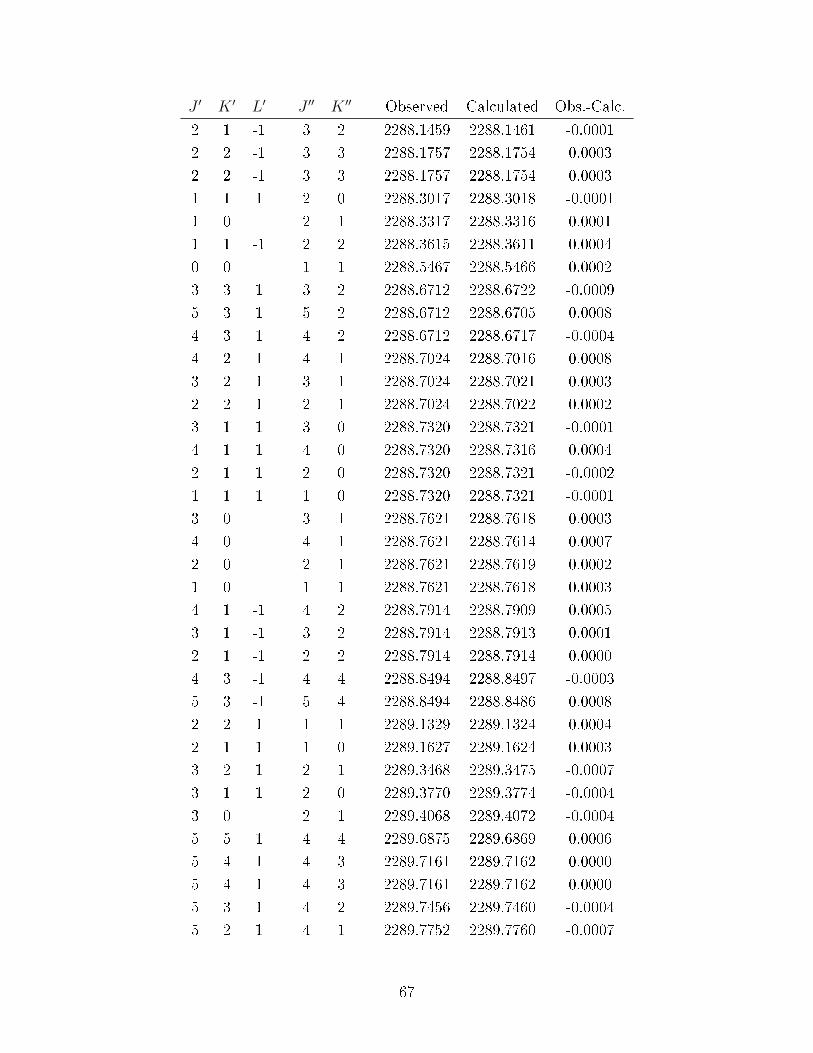
J ′ K ′ L′ J ′′ K ′′ Observed Calculated Obs.-Calc.2 1 -1 3 2 2288.1459 2288.1461 -0.00012 2 -1 3 3 2288.1757 2288.1754 0.00032 2 -1 3 3 2288.1757 2288.1754 0.00031 1 1 2 0 2288.3017 2288.3018 -0.00011 0 2 1 2288.3317 2288.3316 0.00011 1 -1 2 2 2288.3615 2288.3611 0.00040 0 1 1 2288.5467 2288.5466 0.00023 3 1 3 2 2288.6712 2288.6722 -0.00095 3 1 5 2 2288.6712 2288.6705 0.00084 3 1 4 2 2288.6712 2288.6717 -0.00044 2 1 4 1 2288.7024 2288.7016 0.00083 2 1 3 1 2288.7024 2288.7021 0.00032 2 1 2 1 2288.7024 2288.7022 0.00023 1 1 3 0 2288.7320 2288.7321 -0.00014 1 1 4 0 2288.7320 2288.7316 0.00042 1 1 2 0 2288.7320 2288.7321 -0.00021 1 1 1 0 2288.7320 2288.7321 -0.00013 0 3 1 2288.7621 2288.7618 0.00034 0 4 1 2288.7621 2288.7614 0.00072 0 2 1 2288.7621 2288.7619 0.00021 0 1 1 2288.7621 2288.7618 0.00034 1 -1 4 2 2288.7914 2288.7909 0.00053 1 -1 3 2 2288.7914 2288.7913 0.00012 1 -1 2 2 2288.7914 2288.7914 0.00004 3 -1 4 4 2288.8494 2288.8497 -0.00035 3 -1 5 4 2288.8494 2288.8486 0.00082 2 1 1 1 2289.1329 2289.1324 0.00042 1 1 1 0 2289.1627 2289.1624 0.00033 2 1 2 1 2289.3468 2289.3475 -0.00073 1 1 2 0 2289.3770 2289.3774 -0.00043 0 2 1 2289.4068 2289.4072 -0.00045 5 1 4 4 2289.6875 2289.6869 0.00065 4 1 4 3 2289.7161 2289.7162 0.00005 4 1 4 3 2289.7161 2289.7162 0.00005 3 1 4 2 2289.7456 2289.7460 -0.00045 2 1 4 1 2289.7752 2289.7760 -0.0007
67
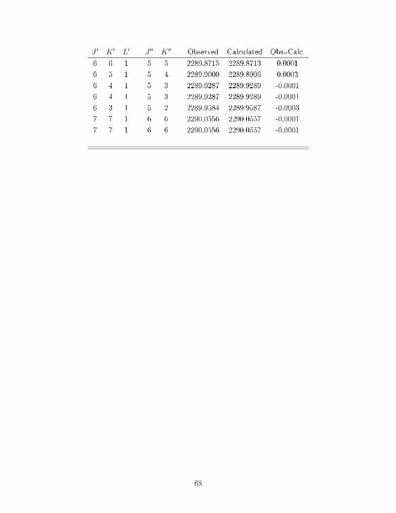
J ′ K ′ L′ J ′′ K ′′ Observed Calculated Obs.-Calc.6 6 1 5 5 2289.8715 2289.8713 0.00016 5 1 5 4 2289.9000 2289.8996 0.00036 4 1 5 3 2289.9287 2289.9289 -0.00016 4 1 5 3 2289.9287 2289.9289 -0.00016 3 1 5 2 2289.9584 2289.9587 -0.00037 7 1 6 6 2290.0556 2290.0557 -0.00017 7 1 6 6 2290.0556 2290.0557 -0.0001
68

Table A.2: Observed transitions in the ν2 + ν13 and ν12 bands of C6D
6−Ne.
J ′ K ′ L′ J ′′ K ′′ Observed Calculated Obs.-Calc.5 5 -1 6 6 2274.7295 2274.7303 -0.00075 5 -1 6 6 2274.7295 2274.7303 -0.00074 4 -1 5 5 2274.9418 2274.9413 0.00045 2 -1 6 3 2275.0301 2275.0276 0.00255 2 -1 6 3 2275.0301 2275.0276 0.00254 3 -1 5 4 2275.0393 2275.0405 -0.00123 3 -1 4 4 2275.1530 2275.1525 0.00054 1 -1 5 2 2275.2361 2275.2384 -0.00233 2 -1 4 3 2275.2513 2275.2516 -0.00033 2 -1 4 3 2275.2513 2275.2516 -0.00032 2 -1 3 3 2275.3644 2275.3637 0.00072 2 -1 3 3 2275.3644 2275.3637 0.00071 1 -1 2 2 2275.5750 2275.5749 0.00011 1 -1 2 2 2275.5750 2275.5749 0.00019 3 -1 9 4 2275.6017 2275.6024 -0.00066 3 -1 6 4 2275.6017 2275.6017 0.00014 3 -1 4 4 2275.6017 2275.6014 0.00047 3 -1 7 4 2275.6017 2275.6019 -0.00015 3 -1 5 4 2275.6017 2275.6015 0.00028 3 -1 8 4 2275.6017 2275.6021 -0.000410 3 -1 10 4 2275.6017 2275.6027 -0.00091 0 2 1 2275.6746 2275.6737 0.00094 2 -1 4 3 2275.7009 2275.7005 0.00036 2 -1 6 3 2275.7009 2275.7008 0.00015 2 -1 5 3 2275.7009 2275.7006 0.00027 2 -1 7 3 2275.7009 2275.7009 0.00008 2 -1 8 3 2275.7009 2275.7010 -0.00028 2 -1 8 3 2275.7009 2275.7010 -0.00024 2 -1 4 3 2275.7009 2275.7005 0.00036 2 -1 6 3 2275.7009 2275.7008 0.00015 2 -1 5 3 2275.7009 2275.7006 0.00027 2 -1 7 3 2275.7009 2275.7009 0.00009 1 -1 9 2 2275.7998 2275.7999 0.000010 1 -1 10 2 2275.7998 2275.8000 -0.00016 1 -1 6 2 2275.7998 2275.7996 0.0002
69

J ′ K ′ L′ J ′′ K ′′ Observed Calculated Obs.-Calc.5 1 -1 5 2 2275.7998 2275.7996 0.00023 1 -1 3 2 2275.7998 2275.7995 0.00038 1 -1 8 2 2275.7998 2275.7998 0.00004 1 -1 4 2 2275.7998 2275.7995 0.00037 1 -1 7 2 2275.7998 2275.7997 0.00017 0 7 1 2275.8984 2275.8983 0.00019 0 9 1 2275.8984 2275.8983 0.00018 0 8 1 2275.8984 2275.8983 0.000110 0 10 1 2275.8984 2275.8983 0.00016 0 6 1 2275.8984 2275.8983 0.00015 0 5 1 2275.8984 2275.8983 0.00013 0 3 1 2275.8984 2275.8983 0.00014 0 4 1 2275.8984 2275.8983 0.00013 1 1 3 0 2275.9962 2275.9969 -0.00076 1 1 6 0 2275.9962 2275.9967 -0.00059 1 1 9 0 2275.9962 2275.9965 -0.00037 1 1 7 0 2275.9962 2275.9967 -0.00044 1 1 4 0 2275.9962 2275.9968 -0.00068 1 1 8 0 2275.9962 2275.9966 -0.000410 1 1 10 0 2275.9962 2275.9964 -0.00025 1 1 5 0 2275.9962 2275.9968 -0.00063 2 1 3 1 2276.0947 2276.0952 -0.00052 2 1 2 1 2276.0947 2276.0953 -0.00069 2 1 9 1 2276.0947 2276.0945 0.000210 2 1 10 1 2276.0947 2276.0943 0.00047 2 1 7 1 2276.0947 2276.0948 -0.00014 2 1 4 1 2276.0947 2276.0952 -0.00045 2 1 5 1 2276.0947 2276.0951 -0.00036 2 1 6 1 2276.0947 2276.0950 -0.00021 1 1 0 0 2276.1099 2276.1092 0.00062 1 1 1 0 2276.2219 2276.2215 0.00043 0 2 1 2276.2356 2276.2351 0.00043 2 1 2 1 2276.4306 2276.4321 -0.00154 1 1 3 0 2276.4435 2276.4459 -0.00243 3 1 2 2 2276.5264 2276.5302 -0.00384 2 1 3 1 2276.5374 2276.5442 -0.0068
70
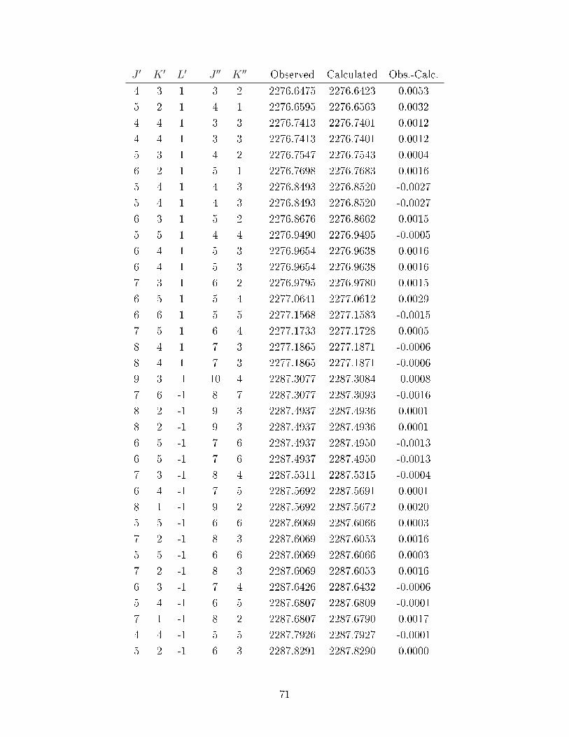
J ′ K ′ L′ J ′′ K ′′ Observed Calculated Obs.-Calc.4 3 1 3 2 2276.6475 2276.6423 0.00535 2 1 4 1 2276.6595 2276.6563 0.00324 4 1 3 3 2276.7413 2276.7401 0.00124 4 1 3 3 2276.7413 2276.7401 0.00125 3 1 4 2 2276.7547 2276.7543 0.00046 2 1 5 1 2276.7698 2276.7683 0.00165 4 1 4 3 2276.8493 2276.8520 -0.00275 4 1 4 3 2276.8493 2276.8520 -0.00276 3 1 5 2 2276.8676 2276.8662 0.00155 5 1 4 4 2276.9490 2276.9495 -0.00056 4 1 5 3 2276.9654 2276.9638 0.00166 4 1 5 3 2276.9654 2276.9638 0.00167 3 1 6 2 2276.9795 2276.9780 0.00156 5 1 5 4 2277.0641 2277.0612 0.00296 6 1 5 5 2277.1568 2277.1583 -0.00157 5 1 6 4 2277.1733 2277.1728 0.00058 4 1 7 3 2277.1865 2277.1871 -0.00068 4 1 7 3 2277.1865 2277.1871 -0.00069 3 -1 10 4 2287.3077 2287.3084 -0.00087 6 -1 8 7 2287.3077 2287.3093 -0.00168 2 -1 9 3 2287.4937 2287.4936 0.00018 2 -1 9 3 2287.4937 2287.4936 0.00016 5 -1 7 6 2287.4937 2287.4950 -0.00136 5 -1 7 6 2287.4937 2287.4950 -0.00137 3 -1 8 4 2287.5311 2287.5315 -0.00046 4 -1 7 5 2287.5692 2287.5691 0.00018 1 -1 9 2 2287.5692 2287.5672 0.00205 5 -1 6 6 2287.6069 2287.6066 0.00037 2 -1 8 3 2287.6069 2287.6053 0.00165 5 -1 6 6 2287.6069 2287.6066 0.00037 2 -1 8 3 2287.6069 2287.6053 0.00166 3 -1 7 4 2287.6426 2287.6432 -0.00065 4 -1 6 5 2287.6807 2287.6809 -0.00017 1 -1 8 2 2287.6807 2287.6790 0.00174 4 -1 5 5 2287.7926 2287.7927 -0.00015 2 -1 6 3 2287.8291 2287.8290 0.0000
71
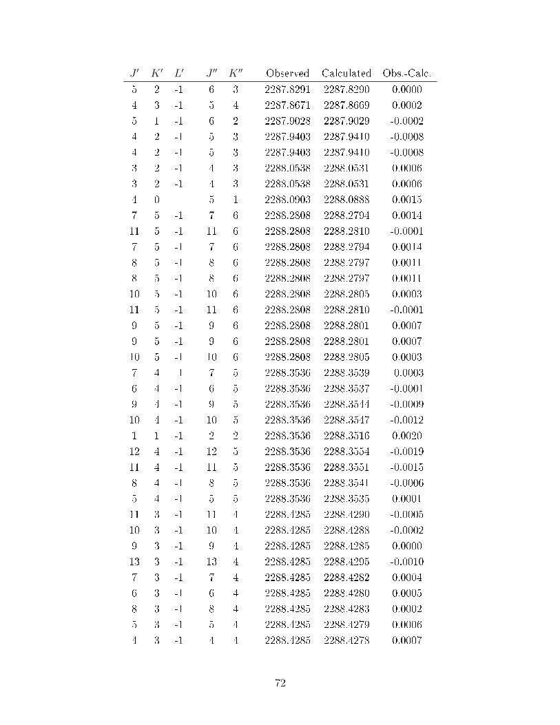
J ′ K ′ L′ J ′′ K ′′ Observed Calculated Obs.-Calc.5 2 -1 6 3 2287.8291 2287.8290 0.00004 3 -1 5 4 2287.8671 2287.8669 0.00025 1 -1 6 2 2287.9028 2287.9029 -0.00024 2 -1 5 3 2287.9403 2287.9410 -0.00084 2 -1 5 3 2287.9403 2287.9410 -0.00083 2 -1 4 3 2288.0538 2288.0531 0.00063 2 -1 4 3 2288.0538 2288.0531 0.00064 0 5 1 2288.0903 2288.0888 0.00157 5 -1 7 6 2288.2808 2288.2794 0.001411 5 -1 11 6 2288.2808 2288.2810 -0.00017 5 -1 7 6 2288.2808 2288.2794 0.00148 5 -1 8 6 2288.2808 2288.2797 0.00118 5 -1 8 6 2288.2808 2288.2797 0.001110 5 -1 10 6 2288.2808 2288.2805 0.000311 5 -1 11 6 2288.2808 2288.2810 -0.00019 5 -1 9 6 2288.2808 2288.2801 0.00079 5 -1 9 6 2288.2808 2288.2801 0.000710 5 -1 10 6 2288.2808 2288.2805 0.00037 4 -1 7 5 2288.3536 2288.3539 -0.00036 4 -1 6 5 2288.3536 2288.3537 -0.00019 4 -1 9 5 2288.3536 2288.3544 -0.000910 4 -1 10 5 2288.3536 2288.3547 -0.00121 1 -1 2 2 2288.3536 2288.3516 0.002012 4 -1 12 5 2288.3536 2288.3554 -0.001911 4 -1 11 5 2288.3536 2288.3551 -0.00158 4 -1 8 5 2288.3536 2288.3541 -0.00065 4 -1 5 5 2288.3536 2288.3535 0.000111 3 -1 11 4 2288.4285 2288.4290 -0.000510 3 -1 10 4 2288.4285 2288.4288 -0.00029 3 -1 9 4 2288.4285 2288.4285 0.000013 3 -1 13 4 2288.4285 2288.4295 -0.00107 3 -1 7 4 2288.4285 2288.4282 0.00046 3 -1 6 4 2288.4285 2288.4280 0.00058 3 -1 8 4 2288.4285 2288.4283 0.00025 3 -1 5 4 2288.4285 2288.4279 0.00064 3 -1 4 4 2288.4285 2288.4278 0.0007
72
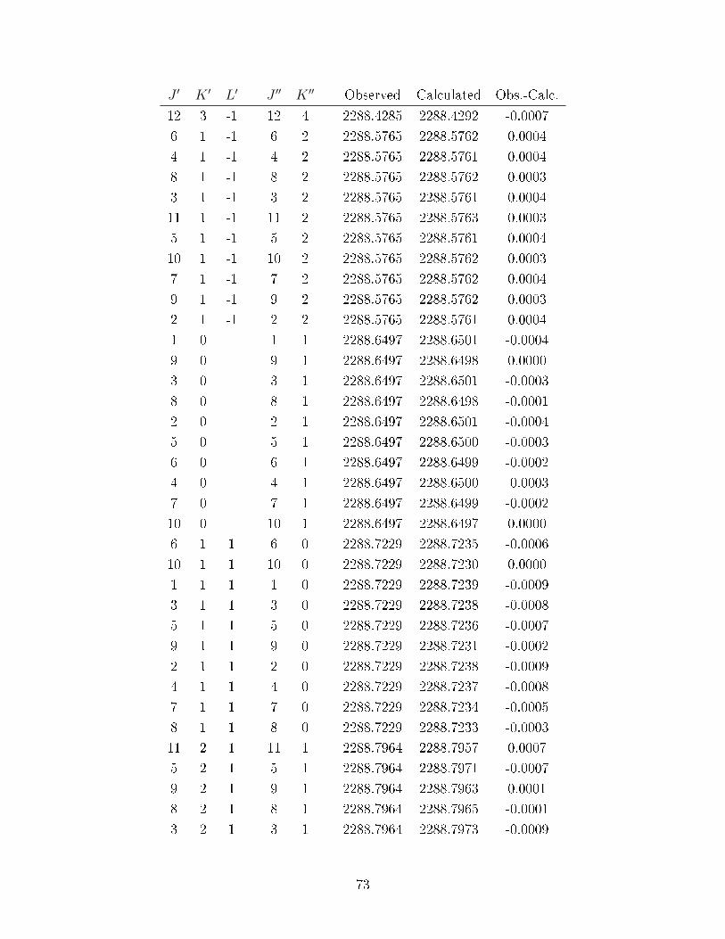
J ′ K ′ L′ J ′′ K ′′ Observed Calculated Obs.-Calc.12 3 -1 12 4 2288.4285 2288.4292 -0.00076 1 -1 6 2 2288.5765 2288.5762 0.00044 1 -1 4 2 2288.5765 2288.5761 0.00048 1 -1 8 2 2288.5765 2288.5762 0.00033 1 -1 3 2 2288.5765 2288.5761 0.000411 1 -1 11 2 2288.5765 2288.5763 0.00035 1 -1 5 2 2288.5765 2288.5761 0.000410 1 -1 10 2 2288.5765 2288.5762 0.00037 1 -1 7 2 2288.5765 2288.5762 0.00049 1 -1 9 2 2288.5765 2288.5762 0.00032 1 -1 2 2 2288.5765 2288.5761 0.00041 0 1 1 2288.6497 2288.6501 -0.00049 0 9 1 2288.6497 2288.6498 0.00003 0 3 1 2288.6497 2288.6501 -0.00038 0 8 1 2288.6497 2288.6498 -0.00012 0 2 1 2288.6497 2288.6501 -0.00045 0 5 1 2288.6497 2288.6500 -0.00036 0 6 1 2288.6497 2288.6499 -0.00024 0 4 1 2288.6497 2288.6500 -0.00037 0 7 1 2288.6497 2288.6499 -0.000210 0 10 1 2288.6497 2288.6497 0.00006 1 1 6 0 2288.7229 2288.7235 -0.000610 1 1 10 0 2288.7229 2288.7230 0.00001 1 1 1 0 2288.7229 2288.7239 -0.00093 1 1 3 0 2288.7229 2288.7238 -0.00085 1 1 5 0 2288.7229 2288.7236 -0.00079 1 1 9 0 2288.7229 2288.7231 -0.00022 1 1 2 0 2288.7229 2288.7238 -0.00094 1 1 4 0 2288.7229 2288.7237 -0.00087 1 1 7 0 2288.7229 2288.7234 -0.00058 1 1 8 0 2288.7229 2288.7233 -0.000311 2 1 11 1 2288.7964 2288.7957 0.00075 2 1 5 1 2288.7964 2288.7971 -0.00079 2 1 9 1 2288.7964 2288.7963 0.00018 2 1 8 1 2288.7964 2288.7965 -0.00013 2 1 3 1 2288.7964 2288.7973 -0.0009
73

J ′ K ′ L′ J ′′ K ′′ Observed Calculated Obs.-Calc.6 2 1 6 1 2288.7964 2288.7969 -0.00054 2 1 4 1 2288.7964 2288.7972 -0.00087 2 1 7 1 2288.7964 2288.7968 -0.00032 2 1 2 1 2288.7964 2288.7974 -0.001010 2 1 10 1 2288.7964 2288.7960 0.000410 3 1 10 2 2288.8695 2288.8689 0.00069 3 1 9 2 2288.8695 2288.8693 0.000212 3 1 12 2 2288.8695 2288.8681 0.00143 3 1 3 2 2288.8695 2288.8707 -0.001211 3 1 11 2 2288.8695 2288.8685 0.00105 3 1 5 2 2288.8695 2288.8704 -0.00097 3 1 7 2 2288.8695 2288.8699 -0.00048 3 1 8 2 2288.8695 2288.8696 -0.00016 3 1 6 2 2288.8695 2288.8702 -0.00074 3 1 4 2 2288.8695 2288.8706 -0.00114 3 1 3 2 2289.3198 2289.3195 0.00034 4 1 3 3 2289.3935 2289.3926 0.00094 4 1 3 3 2289.3935 2289.3926 0.00095 3 1 4 2 2289.4319 2289.4315 0.00045 5 1 4 4 2289.5783 2289.5772 0.0011
74
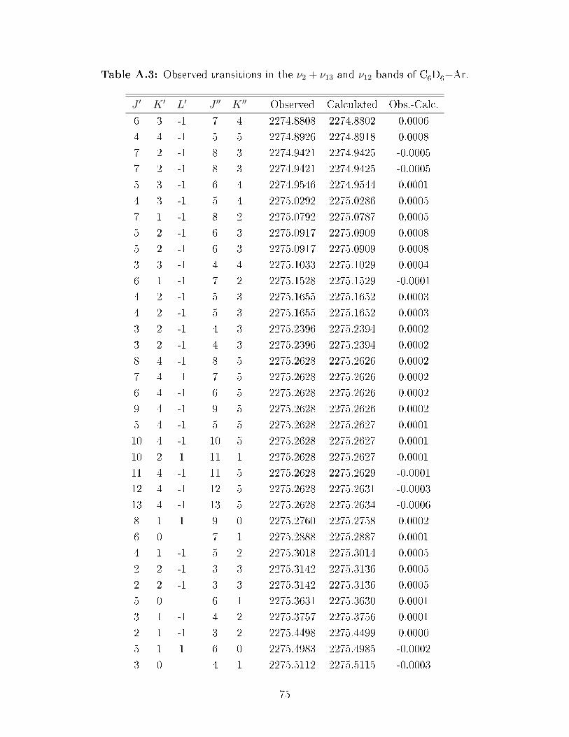
Table A.3: Observed transitions in the ν2 + ν13 and ν12 bands of C6D
6−Ar.
J ′ K ′ L′ J ′′ K ′′ Observed Calculated Obs.-Calc.6 3 -1 7 4 2274.8808 2274.8802 0.00064 4 -1 5 5 2274.8926 2274.8918 0.00087 2 -1 8 3 2274.9421 2274.9425 -0.00057 2 -1 8 3 2274.9421 2274.9425 -0.00055 3 -1 6 4 2274.9546 2274.9544 0.00014 3 -1 5 4 2275.0292 2275.0286 0.00057 1 -1 8 2 2275.0792 2275.0787 0.00055 2 -1 6 3 2275.0917 2275.0909 0.00085 2 -1 6 3 2275.0917 2275.0909 0.00083 3 -1 4 4 2275.1033 2275.1029 0.00046 1 -1 7 2 2275.1528 2275.1529 -0.00014 2 -1 5 3 2275.1655 2275.1652 0.00034 2 -1 5 3 2275.1655 2275.1652 0.00033 2 -1 4 3 2275.2396 2275.2394 0.00023 2 -1 4 3 2275.2396 2275.2394 0.00028 4 -1 8 5 2275.2628 2275.2626 0.00027 4 -1 7 5 2275.2628 2275.2626 0.00026 4 -1 6 5 2275.2628 2275.2626 0.00029 4 -1 9 5 2275.2628 2275.2626 0.00025 4 -1 5 5 2275.2628 2275.2627 0.000110 4 -1 10 5 2275.2628 2275.2627 0.000110 2 1 11 1 2275.2628 2275.2627 0.000111 4 -1 11 5 2275.2628 2275.2629 -0.000112 4 -1 12 5 2275.2628 2275.2631 -0.000313 4 -1 13 5 2275.2628 2275.2634 -0.00068 1 1 9 0 2275.2760 2275.2758 0.00026 0 7 1 2275.2888 2275.2887 0.00014 1 -1 5 2 2275.3018 2275.3014 0.00052 2 -1 3 3 2275.3142 2275.3136 0.00052 2 -1 3 3 2275.3142 2275.3136 0.00055 0 6 1 2275.3631 2275.3630 0.00013 1 -1 4 2 2275.3757 2275.3756 0.00012 1 -1 3 2 2275.4498 2275.4499 0.00005 1 1 6 0 2275.4983 2275.4985 -0.00023 0 4 1 2275.5112 2275.5115 -0.0003
75

J ′ K ′ L′ J ′′ K ′′ Observed Calculated Obs.-Calc.1 1 -1 2 2 2275.5242 2275.5241 0.00018 2 -1 8 3 2275.5352 2275.5360 -0.00088 2 -1 8 3 2275.5352 2275.5360 -0.00087 2 -1 7 3 2275.5352 2275.5360 -0.00087 2 -1 7 3 2275.5352 2275.5360 -0.00086 2 -1 6 3 2275.5352 2275.5360 -0.00086 2 -1 6 3 2275.5352 2275.5360 -0.00085 2 -1 5 3 2275.5352 2275.5361 -0.00095 2 -1 5 3 2275.5352 2275.5361 -0.00094 2 -1 4 3 2275.5352 2275.5361 -0.00094 2 -1 4 3 2275.5352 2275.5361 -0.00094 1 1 5 0 2275.5727 2275.5728 -0.00012 0 3 1 2275.5860 2275.5858 0.00021 0 2 1 2275.6602 2275.6600 0.00029 1 -1 9 2 2275.6724 2275.6721 0.00028 1 -1 8 2 2275.6724 2275.6722 0.00027 1 -1 7 2 2275.6724 2275.6722 0.000210 1 -1 10 2 2275.6724 2275.6722 0.00026 1 -1 6 2 2275.6724 2275.6722 0.000111 1 -1 11 2 2275.6724 2275.6723 0.00015 1 -1 5 2 2275.6724 2275.6723 0.00014 1 -1 4 2 2275.6724 2275.6724 0.00003 1 -1 3 2 2275.6724 2275.6724 -0.00012 1 -1 2 2 2275.6724 2275.6725 -0.00019 0 9 1 2275.8083 2275.8080 0.00048 0 8 1 2275.8083 2275.8080 0.000310 0 10 1 2275.8083 2275.8080 0.00037 0 7 1 2275.8083 2275.8080 0.00036 0 6 1 2275.8083 2275.8081 0.00025 0 5 1 2275.8083 2275.8082 0.00024 0 4 1 2275.8083 2275.8083 0.00013 0 3 1 2275.8083 2275.8083 0.00002 0 2 1 2275.8083 2275.8084 0.00001 0 1 1 2275.8083 2275.8084 -0.00019 1 1 9 0 2275.9437 2275.9435 0.000210 1 1 10 0 2275.9437 2275.9435 0.0002
76

J ′ K ′ L′ J ′′ K ′′ Observed Calculated Obs.-Calc.8 1 1 8 0 2275.9437 2275.9435 0.00027 1 1 7 0 2275.9437 2275.9436 0.00016 1 1 6 0 2275.9437 2275.9437 0.00005 1 1 5 0 2275.9437 2275.9437 0.00004 1 1 4 0 2275.9437 2275.9438 -0.00013 1 1 3 0 2275.9437 2275.9439 -0.00022 1 1 2 0 2275.9437 2275.9440 -0.00031 1 1 1 0 2275.9437 2275.9440 -0.000310 2 1 10 1 2276.0788 2276.0786 0.00029 2 1 9 1 2276.0788 2276.0786 0.000211 2 1 11 1 2276.0788 2276.0786 0.00028 2 1 8 1 2276.0788 2276.0787 0.00017 2 1 7 1 2276.0788 2276.0788 0.00006 2 1 6 1 2276.0788 2276.0789 0.00005 2 1 5 1 2276.0788 2276.0790 -0.00014 2 1 4 1 2276.0788 2276.0791 -0.00023 2 1 3 1 2276.0788 2276.0791 -0.00032 2 1 2 1 2276.0788 2276.0792 -0.00042 1 1 1 0 2276.0925 2276.0924 0.00014 0 3 1 2276.1051 2276.1051 0.000010 3 1 10 2 2276.2136 2276.2134 0.000211 3 1 11 2 2276.2136 2276.2134 0.00029 3 1 9 2 2276.2136 2276.2134 0.000112 3 1 12 2 2276.2136 2276.2135 0.00018 3 1 8 2 2276.2136 2276.2135 0.00007 3 1 7 2 2276.2136 2276.2136 -0.00016 3 1 6 2 2276.2136 2276.2137 -0.00025 3 1 5 2 2276.2136 2276.2139 -0.00034 3 1 4 2 2276.2136 2276.2140 -0.00043 3 1 3 2 2276.2136 2276.2141 -0.00052 2 1 1 1 2276.2276 2276.2276 0.00004 1 1 3 0 2276.2408 2276.2407 0.00013 2 1 2 1 2276.3020 2276.3018 0.00025 1 1 4 0 2276.3150 2276.3148 0.00029 4 1 9 3 2276.3481 2276.3479 0.00029 4 1 9 3 2276.3481 2276.3479 0.0002
77
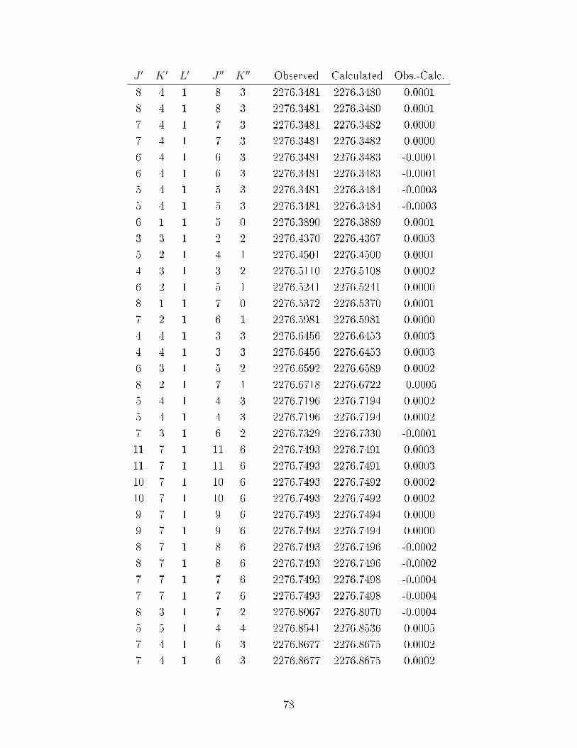
J ′ K ′ L′ J ′′ K ′′ Observed Calculated Obs.-Calc.8 4 1 8 3 2276.3481 2276.3480 0.00018 4 1 8 3 2276.3481 2276.3480 0.00017 4 1 7 3 2276.3481 2276.3482 0.00007 4 1 7 3 2276.3481 2276.3482 0.00006 4 1 6 3 2276.3481 2276.3483 -0.00016 4 1 6 3 2276.3481 2276.3483 -0.00015 4 1 5 3 2276.3481 2276.3484 -0.00035 4 1 5 3 2276.3481 2276.3484 -0.00036 1 1 5 0 2276.3890 2276.3889 0.00013 3 1 2 2 2276.4370 2276.4367 0.00035 2 1 4 1 2276.4501 2276.4500 0.00014 3 1 3 2 2276.5110 2276.5108 0.00026 2 1 5 1 2276.5241 2276.5241 0.00008 1 1 7 0 2276.5372 2276.5370 0.00017 2 1 6 1 2276.5981 2276.5981 0.00004 4 1 3 3 2276.6456 2276.6453 0.00034 4 1 3 3 2276.6456 2276.6453 0.00036 3 1 5 2 2276.6592 2276.6589 0.00028 2 1 7 1 2276.6718 2276.6722 -0.00055 4 1 4 3 2276.7196 2276.7194 0.00025 4 1 4 3 2276.7196 2276.7194 0.00027 3 1 6 2 2276.7329 2276.7330 -0.000111 7 1 11 6 2276.7493 2276.7491 0.000311 7 1 11 6 2276.7493 2276.7491 0.000310 7 1 10 6 2276.7493 2276.7492 0.000210 7 1 10 6 2276.7493 2276.7492 0.00029 7 1 9 6 2276.7493 2276.7494 0.00009 7 1 9 6 2276.7493 2276.7494 0.00008 7 1 8 6 2276.7493 2276.7496 -0.00028 7 1 8 6 2276.7493 2276.7496 -0.00027 7 1 7 6 2276.7493 2276.7498 -0.00047 7 1 7 6 2276.7493 2276.7498 -0.00048 3 1 7 2 2276.8067 2276.8070 -0.00045 5 1 4 4 2276.8541 2276.8536 0.00057 4 1 6 3 2276.8677 2276.8675 0.00027 4 1 6 3 2276.8677 2276.8675 0.0002
78

J ′ K ′ L′ J ′′ K ′′ Observed Calculated Obs.-Calc.6 5 1 5 4 2276.9279 2276.9276 0.00028 4 1 7 3 2276.9413 2276.9415 -0.00028 4 1 7 3 2276.9413 2276.9415 -0.000210 3 1 9 2 2276.9543 2276.9551 -0.00084 3 -1 5 4 2287.7860 2287.7864 -0.00047 1 -1 8 2 2287.7860 2287.7873 -0.00133 3 -1 4 4 2287.8613 2287.8605 0.00086 1 -1 7 2 2287.8613 2287.8614 -0.00014 2 -1 5 3 2287.8983 2287.8981 0.00024 2 -1 5 3 2287.8983 2287.8981 0.00027 0 8 1 2287.8983 2287.8988 -0.00053 2 -1 4 3 2287.9722 2287.9722 0.00003 2 -1 4 3 2287.9722 2287.9722 0.00006 0 7 1 2287.9722 2287.9729 -0.00074 1 -1 5 2 2288.0094 2288.0097 -0.00027 1 1 8 0 2288.0094 2288.0103 -0.00085 4 -1 5 5 2288.0462 2288.0456 0.00066 4 -1 6 5 2288.0462 2288.0457 0.00057 4 -1 7 5 2288.0462 2288.0458 0.00048 4 -1 8 5 2288.0462 2288.0459 0.00039 4 -1 9 5 2288.0462 2288.0461 0.000110 4 -1 10 5 2288.0462 2288.0463 -0.00012 2 -1 3 3 2288.0462 2288.0464 -0.00022 2 -1 3 3 2288.0462 2288.0464 -0.00025 0 6 1 2288.0462 2288.0471 -0.00098 2 1 9 1 2288.0462 2288.0476 -0.00143 1 -1 4 2 2288.0837 2288.0839 -0.00026 1 1 7 0 2288.0837 2288.0844 -0.00084 3 -1 4 4 2288.1573 2288.1573 0.00005 3 -1 5 4 2288.1573 2288.1574 -0.00016 3 -1 6 4 2288.1573 2288.1574 -0.00017 3 -1 7 4 2288.1573 2288.1575 -0.00028 3 -1 8 4 2288.1573 2288.1576 -0.00039 3 -1 9 4 2288.1573 2288.1578 -0.000510 3 -1 10 4 2288.1573 2288.1580 -0.00072 1 -1 3 2 2288.1573 2288.1581 -0.0008
79
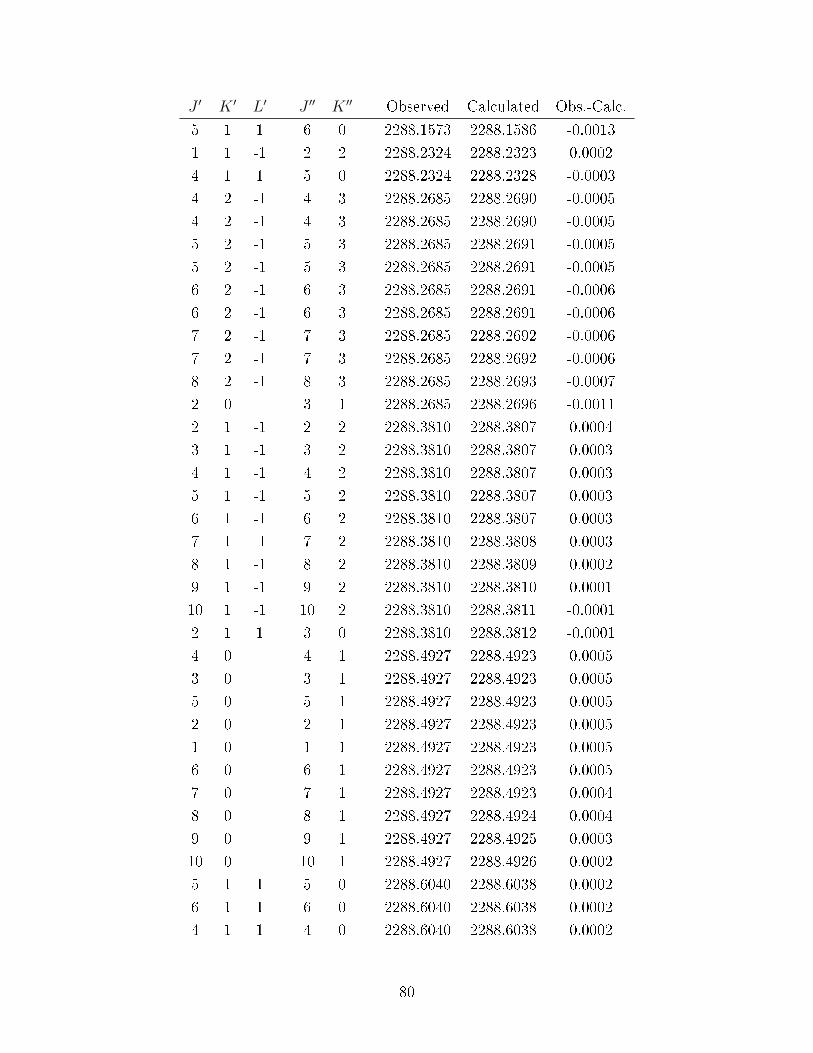
J ′ K ′ L′ J ′′ K ′′ Observed Calculated Obs.-Calc.5 1 1 6 0 2288.1573 2288.1586 -0.00131 1 -1 2 2 2288.2324 2288.2323 0.00024 1 1 5 0 2288.2324 2288.2328 -0.00034 2 -1 4 3 2288.2685 2288.2690 -0.00054 2 -1 4 3 2288.2685 2288.2690 -0.00055 2 -1 5 3 2288.2685 2288.2691 -0.00055 2 -1 5 3 2288.2685 2288.2691 -0.00056 2 -1 6 3 2288.2685 2288.2691 -0.00066 2 -1 6 3 2288.2685 2288.2691 -0.00067 2 -1 7 3 2288.2685 2288.2692 -0.00067 2 -1 7 3 2288.2685 2288.2692 -0.00068 2 -1 8 3 2288.2685 2288.2693 -0.00072 0 3 1 2288.2685 2288.2696 -0.00112 1 -1 2 2 2288.3810 2288.3807 0.00043 1 -1 3 2 2288.3810 2288.3807 0.00034 1 -1 4 2 2288.3810 2288.3807 0.00035 1 -1 5 2 2288.3810 2288.3807 0.00036 1 -1 6 2 2288.3810 2288.3807 0.00037 1 -1 7 2 2288.3810 2288.3808 0.00038 1 -1 8 2 2288.3810 2288.3809 0.00029 1 -1 9 2 2288.3810 2288.3810 0.000110 1 -1 10 2 2288.3810 2288.3811 -0.00012 1 1 3 0 2288.3810 2288.3812 -0.00014 0 4 1 2288.4927 2288.4923 0.00053 0 3 1 2288.4927 2288.4923 0.00055 0 5 1 2288.4927 2288.4923 0.00052 0 2 1 2288.4927 2288.4923 0.00051 0 1 1 2288.4927 2288.4923 0.00056 0 6 1 2288.4927 2288.4923 0.00057 0 7 1 2288.4927 2288.4923 0.00048 0 8 1 2288.4927 2288.4924 0.00049 0 9 1 2288.4927 2288.4925 0.000310 0 10 1 2288.4927 2288.4926 0.00025 1 1 5 0 2288.6040 2288.6038 0.00026 1 1 6 0 2288.6040 2288.6038 0.00024 1 1 4 0 2288.6040 2288.6038 0.0002
80
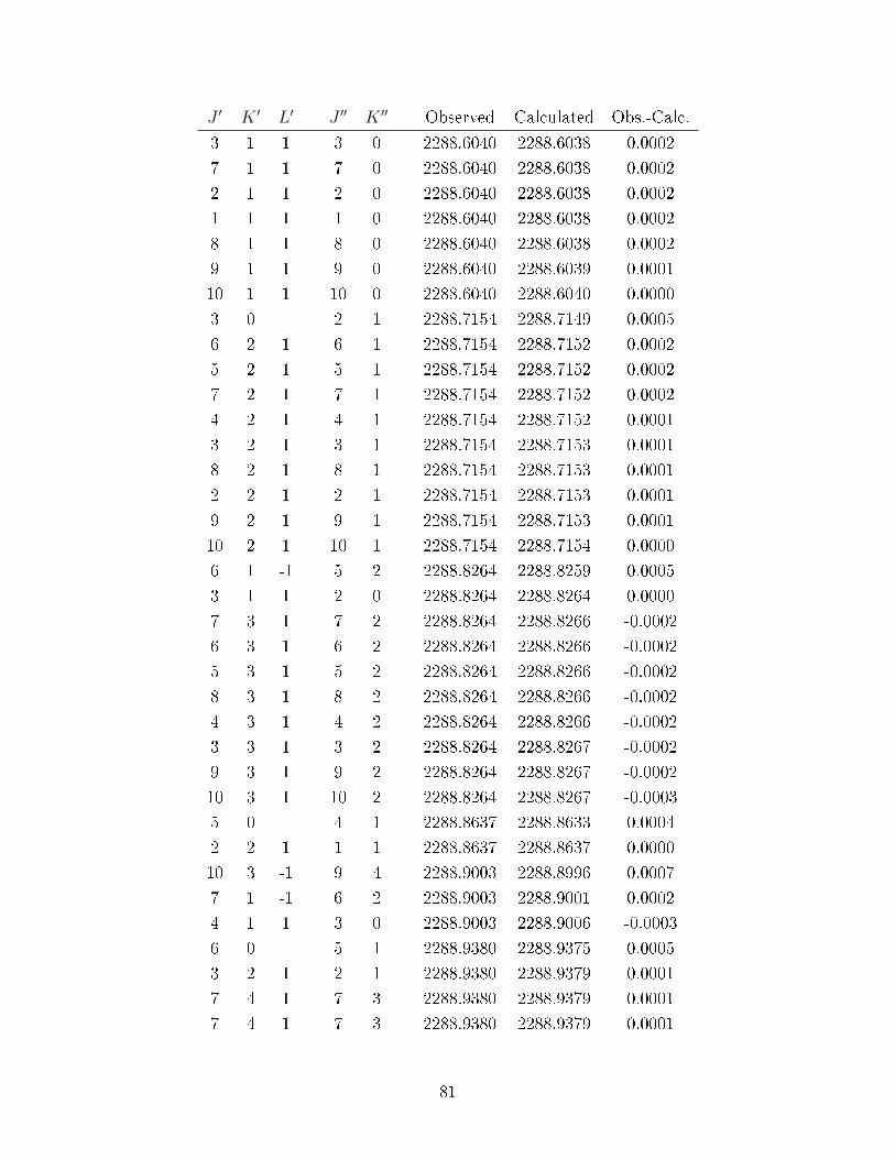
J ′ K ′ L′ J ′′ K ′′ Observed Calculated Obs.-Calc.3 1 1 3 0 2288.6040 2288.6038 0.00027 1 1 7 0 2288.6040 2288.6038 0.00022 1 1 2 0 2288.6040 2288.6038 0.00021 1 1 1 0 2288.6040 2288.6038 0.00028 1 1 8 0 2288.6040 2288.6038 0.00029 1 1 9 0 2288.6040 2288.6039 0.000110 1 1 10 0 2288.6040 2288.6040 0.00003 0 2 1 2288.7154 2288.7149 0.00056 2 1 6 1 2288.7154 2288.7152 0.00025 2 1 5 1 2288.7154 2288.7152 0.00027 2 1 7 1 2288.7154 2288.7152 0.00024 2 1 4 1 2288.7154 2288.7152 0.00013 2 1 3 1 2288.7154 2288.7153 0.00018 2 1 8 1 2288.7154 2288.7153 0.00012 2 1 2 1 2288.7154 2288.7153 0.00019 2 1 9 1 2288.7154 2288.7153 0.000110 2 1 10 1 2288.7154 2288.7154 0.00006 1 -1 5 2 2288.8264 2288.8259 0.00053 1 1 2 0 2288.8264 2288.8264 0.00007 3 1 7 2 2288.8264 2288.8266 -0.00026 3 1 6 2 2288.8264 2288.8266 -0.00025 3 1 5 2 2288.8264 2288.8266 -0.00028 3 1 8 2 2288.8264 2288.8266 -0.00024 3 1 4 2 2288.8264 2288.8266 -0.00023 3 1 3 2 2288.8264 2288.8267 -0.00029 3 1 9 2 2288.8264 2288.8267 -0.000210 3 1 10 2 2288.8264 2288.8267 -0.00035 0 4 1 2288.8637 2288.8633 0.00042 2 1 1 1 2288.8637 2288.8637 0.000010 3 -1 9 4 2288.9003 2288.8996 0.00077 1 -1 6 2 2288.9003 2288.9001 0.00024 1 1 3 0 2288.9003 2288.9006 -0.00036 0 5 1 2288.9380 2288.9375 0.00053 2 1 2 1 2288.9380 2288.9379 0.00017 4 1 7 3 2288.9380 2288.9379 0.00017 4 1 7 3 2288.9380 2288.9379 0.0001
81

J ′ K ′ L′ J ′′ K ′′ Observed Calculated Obs.-Calc.6 4 1 6 3 2288.9380 2288.9379 0.00016 4 1 6 3 2288.9380 2288.9379 0.00015 4 1 5 3 2288.9380 2288.9379 0.00005 4 1 5 3 2288.9380 2288.9379 0.00008 1 -1 7 2 2288.9749 2288.9744 0.00055 1 1 4 0 2288.9749 2288.9748 0.00017 0 6 1 2289.0121 2289.0117 0.00044 2 1 3 1 2289.0121 2289.0121 0.00019 1 -1 8 2 2289.0493 2289.0486 0.00076 1 1 5 0 2289.0493 2289.0490 0.00037 5 1 7 4 2289.0493 2289.0492 0.00018 5 1 8 4 2289.0493 2289.0492 0.00016 5 1 6 4 2289.0493 2289.0492 0.00019 5 1 9 4 2289.0493 2289.0492 0.000110 5 1 10 4 2289.0493 2289.0492 0.00003 3 1 2 2 2289.0493 2289.0493 0.000011 5 1 11 4 2289.0493 2289.0493 -0.000112 5 1 12 4 2289.0493 2289.0495 -0.00028 0 7 1 2289.0865 2289.0859 0.00055 2 1 4 1 2289.0865 2289.0863 0.000210 1 -1 9 2 2289.1237 2289.1228 0.00097 1 1 6 0 2289.1237 2289.1232 0.00054 3 1 3 2 2289.1237 2289.1235 0.000310 0 9 1 2289.2350 2289.2344 0.00067 2 1 6 1 2289.2350 2289.2346 0.00044 4 1 3 3 2289.2350 2289.2348 0.00034 4 1 3 3 2289.2350 2289.2348 0.00039 1 1 8 0 2289.2716 2289.2716 0.00006 3 1 5 2 2289.2716 2289.2718 -0.000211 0 10 1 2289.3089 2289.3086 0.00038 2 1 7 1 2289.3089 2289.3088 0.00025 4 1 4 3 2289.3089 2289.3089 0.00005 4 1 4 3 2289.3089 2289.3089 0.000010 1 1 9 0 2289.3465 2289.3458 0.00077 3 1 6 2 2289.3465 2289.3459 0.00059 8 1 9 7 2289.3829 2289.3826 0.0003
82

J ′ K ′ L′ J ′′ K ′′ Observed Calculated Obs.-Calc.10 8 1 10 7 2289.3829 2289.3826 0.000211 8 1 11 7 2289.3829 2289.3827 0.000112 8 1 12 7 2289.3829 2289.3829 0.000012 0 11 1 2289.3829 2289.3829 -0.00019 2 1 8 1 2289.3829 2289.3830 -0.00016 4 1 5 3 2289.3829 2289.3831 -0.00026 4 1 5 3 2289.3829 2289.3831 -0.000211 1 1 10 0 2289.4201 2289.4201 0.00008 3 1 7 2 2289.4201 2289.4201 0.00005 5 1 4 4 2289.4201 2289.4201 -0.00018 4 1 7 3 2289.5317 2289.5314 0.00038 4 1 7 3 2289.5317 2289.5314 0.000311 2 1 10 1 2289.5317 2289.5314 0.000214 0 13 1 2289.5317 2289.5317 0.00007 5 1 6 4 2289.5678 2289.5684 -0.000610 3 1 9 2 2289.5678 2289.5685 -0.00076 6 1 5 5 2289.6050 2289.6054 -0.00049 4 1 8 3 2289.6050 2289.6055 -0.00059 4 1 8 3 2289.6050 2289.6055 -0.000512 2 1 11 1 2289.6050 2289.6057 -0.0006
83

Appendix B
Supplementary data for Chapter 4
Trimer Complexes
Calculated and observed transitions for C6D
6−He
2, C
6D
6−Ne
2and C
6D
6−Ar
2trimers.
Table B.1: Observed transitions in the ν2 + ν13 (∼ 2275 cm−1) and ν12 (∼ 2288 cm−1)
bands of C6D
6−He
2.
J ′ K ′ L′ J ′′ K ′′ Observed Calculated Obs.-Calc.
2 2 1 1 1 2276.4713 2276.4714 -0.0001
3 3 1 2 2 2276.6808 2276.6809 -0.0001
4 4 1 3 3 2276.8899 2276.8900 -0.0001
0 0 1 1 2275.8915 2275.8911 0.0004
1 0 2 1 2275.7311 2275.7308 0.0003
1 1 -1 2 2 2275.6804 2275.6805 -0.0002
2 1 -1 3 2 2275.5200 2275.5202 -0.0002
2 2 -1 3 3 2275.4695 2275.4696 -0.0000
2 2 -1 3 3 2275.4695 2275.4696 -0.0000
4 1 1 3 0 2276.7409 2276.7405 0.0004
5 2 1 4 1 2276.9493 2276.9491 0.0002
2 1 1 3 0 2275.6204 2275.6206 -0.0002
3 2 -1 4 3 2275.3089 2275.3092 -0.0003
3 3 -1 4 4 2275.2586 2275.2582 0.0004
4 3 -1 5 4 2275.0973 2275.0977 -0.0004
4 4 -1 5 5 2275.0465 2275.0464 0.0001
5 5 1 4 4 2277.0988 2277.0987 0.0001
84

J ′ K ′ L′ J ′′ K ′′ Observed Calculated Obs.-Calc.
6 3 1 5 2 2277.1567 2277.1569 -0.0002
3 0 2 1 2276.5307 2276.5312 -0.0005
4 1 -1 5 2 2275.2000 2275.1996 0.0003
1 1 1 0 0 2288.9163 2288.9163 0.0000
2 2 1 1 1 2289.1022 2289.1021 0.0001
3 1 1 2 0 2289.2360 2289.2365 -0.0005
3 2 1 2 1 2289.2619 2289.2619 0.0000
3 3 1 2 2 2289.2880 2289.2879 0.0001
4 2 1 3 1 2289.4215 2289.4215 -0.0000
4 3 1 3 2 2289.4472 2289.4475 -0.0003
4 4 1 3 3 2289.4735 2289.4735 -0.0000
0 0 1 1 2288.5700 2288.5699 0.0001
1 0 2 1 2288.4097 2288.4095 0.0002
1 1 -1 2 2 2288.3835 2288.3835 -0.0000
2 1 1 3 0 2288.2752 2288.2755 -0.0003
2 0 3 1 2288.2493 2288.2493 0.0001
2 1 -1 3 2 2288.2233 2288.2232 0.0001
2 2 -1 3 3 2288.1968 2288.1971 -0.0003
3 1 -1 4 2 2288.0630 2288.0630 -0.0000
3 3 -1 4 4 2288.0104 2288.0104 -0.0000
5 3 1 4 2 2289.6070 2289.6068 0.0002
5 4 1 4 3 2289.6323 2289.6329 -0.0006
5 5 1 4 4 2289.6592 2289.6590 0.0002
3 2 -1 4 3 2288.0368 2288.0368 0.0001
4 3 -1 5 4 2287.8502 2287.8501 0.0001
85

J ′ K ′ L′ J ′′ K ′′ Observed Calculated Obs.-Calc.
4 4 -1 5 5 2287.8235 2287.8235 -0.0000
6 2 1 5 1 2289.7396 2289.7397 -0.0001
6 3 1 5 2 2289.7661 2289.7658 0.0004
6 4 1 5 3 2289.7918 2289.7920 -0.0001
6 5 1 5 4 2289.8182 2289.8181 0.0001
6 6 1 5 5 2289.8444 2289.8443 0.0001
1 1 1 2 0 2288.4356 2288.4355 0.0001
2 0 1 1 2289.0505 2289.0503 0.0002
3 0 2 1 2289.2101 2289.2100 0.0001
5 2 1 4 1 2289.5810 2289.5807 0.0003
7 4 1 6 3 2289.9505 2289.9507 -0.0001
8 8 1 7 7 2290.2144 2290.2144 -0.0000
86

Table B.2: Observed transitions in the ν2 + ν13 and ν12 bands of C6D
6−Ne
2.
J ′ K ′ L′ J ′′ K ′′ Observed Calculated Obs.-Calc.
5 1 1 4 0 2276.2080 2276.2078 0.0002
2 1 1 1 0 2276.0357 2276.0353 0.0004
1 0 2 1 2275.6540 2275.6540 0.0000
2 0 3 1 2275.5956 2275.5961 -0.0005
4 0 5 1 2275.4795 2275.4796 -0.0001
6 2 1 5 1 2276.4174 2276.4178 -0.0004
3 3 1 2 2 2276.3898 2276.3897 0.0002
4 3 1 3 2 2276.4502 2276.4504 -0.0002
3 1 1 4 0 2275.6883 2275.6887 -0.0003
4 1 1 5 0 2275.6310 2275.6306 0.0004
2 1 -1 3 2 2275.4436 2275.4436 -0.0001
3 1 -1 4 2 2275.3859 2275.3858 0.0001
6 3 1 5 2 2276.5731 2276.5728 0.0003
5 4 1 4 3 2276.6638 2276.6638 0.0000
4 4 1 3 3 2276.5991 2276.5992 -0.0001
6 4 1 5 3 2276.7293 2276.7292 0.0000
2 2 -1 3 3 2275.2891 2275.2889 0.0002
5 5 1 4 4 2276.8162 2276.8163 -0.0001
9 7 1 8 6 2277.4840 2277.4840 -0.0000
4 2 -1 5 3 2275.1752 2275.1752 0.0000
5 1 -1 6 2 2275.2691 2275.2692 -0.0002
1 1 1 0 0 2288.7485 2288.7485 0.0001
3 1 1 2 0 2288.8643 2288.8645 -0.0002
1 0 2 1 2288.4467 2288.4468 -0.0001
87
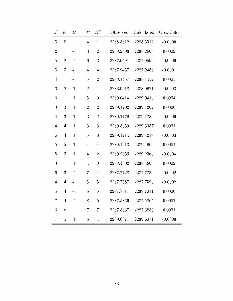
J ′ K ′ L′ J ′′ K ′′ Observed Calculated Obs.-Calc.
3 0 4 1 2288.3312 2288.3312 -0.0000
2 1 -1 3 2 2288.2608 2288.2606 0.0002
5 2 -1 6 3 2287.9591 2287.9592 -0.0000
3 3 -1 4 4 2287.9457 2287.9458 -0.0001
4 1 -1 5 2 2288.1457 2288.1452 0.0005
3 2 1 2 1 2288.9918 2288.9921 -0.0003
6 1 1 5 0 2289.0414 2289.0410 0.0004
3 3 1 2 2 2289.1202 2289.1202 0.0000
4 3 1 3 2 2289.1779 2289.1780 -0.0000
4 4 1 3 3 2289.3059 2289.3057 0.0001
6 4 1 5 3 2289.4214 2289.4218 -0.0003
5 5 1 4 4 2289.4913 2289.4909 0.0004
5 3 1 4 2 2289.2356 2289.2360 -0.0004
3 1 1 4 0 2288.4602 2288.4600 0.0002
6 3 -1 7 4 2287.7728 2287.7730 -0.0002
4 4 -1 5 5 2287.7587 2287.7590 -0.0002
5 4 -1 6 5 2287.7011 2287.7011 0.0000
7 4 -1 8 5 2287.5866 2287.5865 0.0001
6 6 -1 7 7 2287.3837 2287.3836 0.0001
7 5 1 6 4 2289.6071 2289.6071 -0.0000
88

Table B.3: Observed transitions in the ν2 + ν13 and ν12 bands of C6D
6−Ar
2.
J ′ K ′ L′ J ′′ K ′′ Observed Calculated Obs.-Calc.
2 2 1 1 1 2276.1465 2276.1463 0.0002
3 2 1 2 1 2276.1759 2276.1759 -0.0000
3 3 1 2 2 2276.3532 2276.3533 -0.0001
4 3 1 3 2 2276.3826 2276.3828 -0.0003
3 1 1 4 0 2275.7895 2275.7899 -0.0004
4 1 1 5 0 2275.7602 2275.7599 0.0002
6 1 1 7 0 2275.7005 2275.6998 0.0007
3 0 4 1 2275.6118 2275.6117 0.0001
4 0 5 1 2275.5822 2275.5818 0.0004
2 1 -1 3 2 2275.4632 2275.4630 0.0002
5 3 1 4 2 2276.4125 2276.4123 0.0002
8 3 1 7 2 2276.5010 2276.5008 0.0002
9 3 1 8 2 2276.5307 2276.5303 0.0003
10 3 1 9 2 2276.5599 2276.5600 -0.0001
11 3 1 10 2 2276.5888 2276.5897 -0.0008
8 4 1 7 3 2276.6769 2276.6772 -0.0003
9 4 1 8 3 2276.7066 2276.7066 0.0000
7 5 1 6 4 2276.8239 2276.8239 -0.0001
6 6 1 5 5 2276.9708 2276.9706 0.0002
7 2 1 7 1 2276.0855 2276.0857 -0.0002
6 2 1 6 1 2276.0855 2276.0860 -0.0005
8 2 1 8 1 2276.0855 2276.0853 0.0002
6 1 1 6 0 2275.9080 2275.9083 -0.0004
8 1 1 8 0 2275.9080 2275.9078 0.0001
89
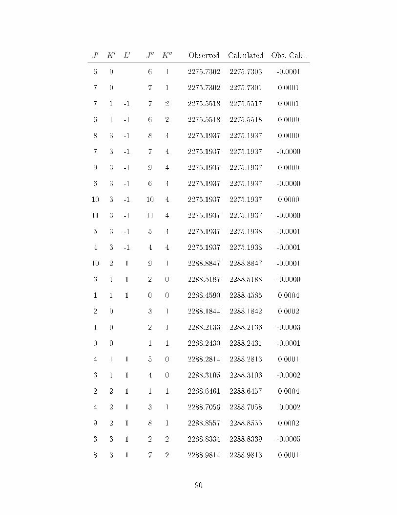
J ′ K ′ L′ J ′′ K ′′ Observed Calculated Obs.-Calc.
6 0 6 1 2275.7302 2275.7303 -0.0001
7 0 7 1 2275.7302 2275.7301 0.0001
7 1 -1 7 2 2275.5518 2275.5517 0.0001
6 1 -1 6 2 2275.5518 2275.5518 0.0000
8 3 -1 8 4 2275.1937 2275.1937 0.0000
7 3 -1 7 4 2275.1937 2275.1937 -0.0000
9 3 -1 9 4 2275.1937 2275.1937 0.0000
6 3 -1 6 4 2275.1937 2275.1937 -0.0000
10 3 -1 10 4 2275.1937 2275.1937 0.0000
11 3 -1 11 4 2275.1937 2275.1937 -0.0000
5 3 -1 5 4 2275.1937 2275.1938 -0.0001
4 3 -1 4 4 2275.1937 2275.1938 -0.0001
10 2 1 9 1 2288.8847 2288.8847 -0.0001
3 1 1 2 0 2288.5187 2288.5188 -0.0000
1 1 1 0 0 2288.4590 2288.4585 0.0004
2 0 3 1 2288.1844 2288.1842 0.0002
1 0 2 1 2288.2133 2288.2136 -0.0003
0 0 1 1 2288.2430 2288.2431 -0.0001
4 1 1 5 0 2288.2814 2288.2813 0.0001
3 1 1 4 0 2288.3105 2288.3106 -0.0002
2 2 1 1 1 2288.6461 2288.6457 0.0004
4 2 1 3 1 2288.7056 2288.7058 -0.0002
9 2 1 8 1 2288.8557 2288.8555 0.0002
3 3 1 2 2 2288.8334 2288.8339 -0.0005
8 3 1 7 2 2288.9814 2288.9813 0.0001
90
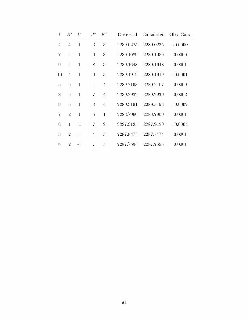
J ′ K ′ L′ J ′′ K ′′ Observed Calculated Obs.-Calc.
4 4 1 3 3 2289.0225 2289.0225 -0.0000
7 4 1 6 3 2289.1089 2289.1089 0.0000
9 4 1 8 3 2289.1648 2289.1648 0.0001
10 4 1 9 3 2289.1919 2289.1919 -0.0001
5 5 1 4 4 2289.2108 2289.2107 0.0000
8 5 1 7 4 2289.2932 2289.2930 0.0002
9 5 1 8 4 2289.3191 2289.3193 -0.0002
7 2 1 6 1 2288.7960 2288.7960 0.0001
6 1 -1 7 2 2287.9125 2287.9129 -0.0004
3 2 -1 4 3 2287.8475 2287.8474 0.0001
6 2 -1 7 3 2287.7594 2287.7593 0.0001
91