The Astrophysical Journal, 754:106 (13pp), 2012 August 1 doi:10.1088/0004-637X/754/2/106C© 2012. The American Astronomical Society. All rights reserved. Printed in the U.S.A.

INFRARED ECLIPSES OF THE STRONGLY IRRADIATED PLANET WASP-33b,AND OSCILLATIONS OF ITS HOST STAR

Drake Deming1,8, Jonathan D. Fraine1,8, Pedro V. Sada2,8, Nikku Madhusudhan3,9, Heather A. Knutson4,Joseph Harrington5, Jasmina Blecic5, Sarah Nymeyer5,10, Alexis M. S. Smith6, and Brian Jackson7

1 Department of Astronomy, University of Maryland, College Park, MD 20742, USA; ddeming@astro.umd.edu2 Department of Mathematics and Physics, Universidad de Monterrey, Monterrey, Mexico

3 Department of Astrophysical Sciences, Princeton University, Princeton, NJ 08544-1001, USA4 Division of Geological and Planetary Sciences, California Institute of Technology, Pasadena, CA 91125, USA

5 Planetary Sciences Group, Department of Physics, University of Central Florida, Orlando, FL 32816-2385, USA6 Astrophysics Group, Keele University, Staffordshire ST5 5BG, UK

7 Department of Terrestrial Magnetism, Carnegie Institution of Washington, Washington, DC 20015, USAReceived 2012 February 8; accepted 2012 May 14; published 2012 July 13

ABSTRACT

We observe two secondary eclipses of the strongly irradiated transiting planet WASP-33b, in the Ks band at 2.15 μm,and one secondary eclipse each at 3.6 μm and 4.5 μm using Warm Spitzer. This planet orbits an A5V δ-Scuti starthat is known to exhibit low-amplitude non-radial p-mode oscillations at about 0.1% semi-amplitude. We detectstellar oscillations in all of our infrared eclipse data, and also in one night of observations at J band (1.25 μm) outof eclipse. The oscillation amplitude, in all infrared bands except Ks, is about the same as in the optical. However,the stellar oscillations in Ks band (2.15 μm) have about twice the amplitude (0.2%) as seen in the optical, possiblybecause the Brackett-γ line falls in this bandpass. As regards the exoplanetary eclipse, we use our best-fit valuesfor the eclipse depth, as well as the 0.9 μm eclipse observed by Smith et al., to explore possible states of theexoplanetary atmosphere, based on the method of Madhusudhan & Seager. On this basis we find two possible statesfor the atmospheric structure of WASP-33b. One possibility is a non-inverted temperature structure in spite of thestrong irradiance, but this model requires an enhanced carbon abundance (C/O > 1). The alternative model hassolar composition, but an inverted temperature structure. Spectroscopy of the planet at secondary eclipse, using aspectral resolution that can resolve the water vapor band structure, should be able to break the degeneracy betweenthese very different possible states of the exoplanetary atmosphere. However, both of those model atmospheresabsorb nearly all of the stellar irradiance with minimal longitudinal re-distribution of energy, strengthening thehypothesis of Cowan & Agol that the most strongly irradiated planets circulate energy poorly. Our measurementof the central phase of the eclipse yields e cos ω = 0.0003 ± 0.00013, which we regard as being consistent with acircular orbit.

Key words: infrared: planetary systems – planets and satellites: atmospheres – planets and satellites: composition– stars: oscillations (including pulsations) – techniques: photometric

Online-only material: color figures

1. INTRODUCTION

Extrasolar planets that orbit close to their stars are subjectto an intense flux of stellar irradiation. The rotation of a veryclose-in planet is expected to become tidally locked to its orbitalperiod on an astrophysically short timescale (Guillot et al. 1996).Consequently, the most close-in exoplanets will receive stellarirradiation exclusively on their star-facing hemispheres. Theresulting heating is believed to be distributed by strong zonalwinds (Showman et al. 2008), but the dynamics of the zonalre-distribution, and therefore the overall energy budget of theplanet, are affected by the vertical temperature structure of theplanetary atmosphere. Many close-in planets exhibit invertedtemperature structures (Knutson et al. 2008; Seager & Deming2010), probably driven by radiative absorption in a high-altitude

8 Visiting Astronomer, Kitt Peak National Observatory, National OpticalAstronomy Observatory, which is operated by the Association of Universitiesfor Research in Astronomy under cooperative agreement with the NationalScience Foundation.9 Current address: Yale Center for Astronomy and Astrophysics, YaleUniversity, New Haven, CT 06511, USA.10 Current address: Department of Earth and Space Sciences, University ofCalifornia at Los Angeles, Los Angeles, CA 90095-1567, USA.

layer of the atmosphere (Burrows et al. 2007). The nature ofthe absorber has been actively discussed (Fortney et al. 2008;Spiegel et al. 2009), but remains unknown.

One promising avenue of investigation is to look for correla-tions between the planetary temperature inversion and the stel-lar flux at ultraviolet (UV) wavelengths (Knutson et al. 2010).Stellar UV radiation has the potential to dissociate absorbingmolecular species, and to create (or destroy) absorbers via pho-tochemistry (Zahnle et al. 2009). The spectral distribution ofUV flux may be critical to the inversion phenomenon. There-fore, it is desirable to investigate planets orbiting strong sourcesof far-UV radiation (i.e., magnetically active stars), as well asplanets receiving irradiation by thermal UV radiation (i.e., hotstars).

An important planet in the latter category is WASP-33b,which orbits an A-type δ-Scuti star with an orbital period of1.22 days (Collier-Cameron et al. 2010; Herrero et al. 2011).The large radius and high temperature of an A-type star producestronger irradiance than would be the case for a solar-type star.Although only an upper limit is available for the mass of WASP-33b (Collier-Cameron et al. 2010), the planet is importantbecause it is among the most strongly irradiated planets. Incontrast to other strongly irradiated planets such as WASP-12

1

The Astrophysical Journal, 754:106 (13pp), 2012 August 1 Deming et al.

(Cowan et al. 2012; Crossfield et al. 2012; Zhao et al. 2012;Campo et al. 2011; Croll et al. 2011; Madhusudhan et al.2011a), little is currently known about the response of WASP-33b to the strong stellar irradiation. Smith et al. (2011) measuredthe thermal emission of WASP-33b from secondary eclipseobservations at 0.9 μm, but there are currently no reporteddetections of the planet at wavelengths longward of 1 μm.

Stellar intensity oscillations of WASP-33 are seen with 0.1%semi-amplitude at optical wavelengths (Herrero et al. 2011).The stellar oscillations may exhibit a greater or lesser amplitudeat infrared (IR) wavelengths. The dependence of the oscillationamplitude on wavelength potentially carries information on thephysics of the oscillations in the stellar atmosphere.

In this paper, we report measurement of the thermal emissionfrom WASP-33b, based on ground-based observations of twosecondary eclipses in the Ks band (2.15 μm), space-borneobservations of eclipses at 3.6 and 4.5 μm by Warm Spitzer,and measurement of the intensity oscillations of the star inall these IR bands, as well as in J band (1.25 μm). Wedescribe the observations and extraction of photometry fromthe data in Sections 2 and 3. In Section 4, we analyze thedata to determine the parameters of the planet’s eclipse andthe oscillatory properties of the star. We explore and discussthe implications of our results in Section 5, and Section 6summarizes our results.

2. OBSERVATIONS

2.1. Ground-based Observations

We observed secondary eclipses of WASP-33b on UT 2011October 10 and 16, using the FLAMINGOS infrared HgCdTeimager at the Cassegrain focus of the 2.1 m telescope at KittPeak National Observatory. The sky on both nights was cloud-less, with excellent photometric conditions prevailing, espe-cially on October 10. The observations used a Ks filter, andwe defocused the telescope so that the diameter of stellar im-ages—measured at the half-intensity level—was 30 pixels (18′′).This substantial defocus improves the photometric precision andphoton-collection efficiency for this bright star (WASP-33 hasV = 8.3). We compensated for drift in the telescope defocus us-ing manual updates at approximately 30 minute intervals, basedon a known formula that relates focus position to temperatureand zenith distance. In that way, we attempted to maintain thegreatest possible image stability.

The 20 × 20 arcmin field of view of FLAMINGOS (2048 ×2048 pixels) provided five comparison stars imaged simultane-ously with WASP-33. We obtained a nearly continuous sequenceof 20 s exposures on each night, amounting to 725 exposureson October 10 and 574 exposures on October 16. Includingthe overhead of reading the detector and writing FITS files, theobservational cadence was 45 s per exposure. We verified thatthe times written to the FITS headers were free of clock er-rors (to about 1 s precision) by comparing the header values tomanual timing made using a web-displayed UT clock. In ad-dition to WASP-33, we observed multiple sky exposures withposition offsets that were used to construct a flat-field frame bymedian-combining the offset sky exposures. We also observeddark frames using the same exposure times as for the stellar andsky-flat observations.

All of our WASP-33 observations used a quad-detector off-axis guide camera, sensitive to optical radiation, and producingreal-time pointing corrections for the telescope. The guiderwas very effective at damping image motion on timescales of

minutes, but differential refraction between the optical and theinfrared leads to a slow drift in stellar positions, amounting toabout 1′′ over 60◦ of zenith distance. This slow positional drifthas only a small effect on our photometry.

During the observations, we noted a significant instabilityin the infrared signal from the FLAMINGOS detector, whichoccurred in response to the changing position of the telescope. Inorder to diagnose and correct for these instabilities, we obtaineda sequence of K-band exposures during the day, with the domeclosed and dark, and the primary mirror cover closed. These2 s exposures measured the thermal emission and scattered lightfrom the telescope mirror cover, and we moved the telescope todifferent positions because the signal instabilities seemed to bea function of telescope position, as described in Section 3.2.

During our WASP-33 observations, we also noticed relativelyprominent intensity oscillations of the star in Ks band. Hence,we also observed 651 consecutive exposures of WASP-33 onthe night of UT October 14, when no eclipse (or transit) of theplanet occurred. This time series was observed using J band andhelps to establish the degree to which the amplitude of stellaroscillations in intensity may depend on wavelength.

2.2. Warm Spitzer Observations

Warm Spitzer observed one eclipse of WASP-33 at 3.6 μm,for 9.6 hr on 2011 March 26, as well as observations of equalduration spanning one eclipse at 4.5 μm on 2011 March 30.The observations were made under the Cycle-6 Target ofOpportunity program (PI: J. Harrington). Both observationsused subarray mode to collect 1264 data cubes, each data cubecomprising 64 exposures of a 32 × 32 pixel section of thedetector. The exposure time was 0.4 s per exposure, and theobservations were not interrupted by any re-pointing.

3. PHOTOMETRY

3.1. Ground-based Photometry

In both Ks and J bands, we subtract a dark frame from eachimage, and divide by the sky flat for that wavelength. Eachsky flat is normalized to have an average value near unity;this facilitates conversion of the observed images from datanumbers to electrons using the known gain of the detectorelectronics (4.9 e/DN). In the limit of large defocus, the starsare essentially images of the telescope’s primary mirror; theyare not well approximated using Gaussians or other functionscommonly used for centroiding. Therefore, we determine thecenter position of each star by exploiting the sharp edges thatare characteristic of the pupil images. Summing the image ofeach star in the X-coordinate produces intensity as a function ofY, I (Y ). The sharp edges of the pupil image will produce peaksin the derivative ∂I/∂Y , one peak at each edge of the image. Wefind those peaks in the spatial derivative, and adopt an averageof the Y-positions of derivative peaks on each side of the I (Y )profile as being the center of the star in Y, and vice versa for X.With the center of each star determined for each exposure, wecalculate the flux in a circular aperture of a given radius centeredon that star.

In addition to WASP-33, we measure 4–6 comparison starson each image. The identification of the comparison stars aregiven in Table 1, with their J and K magnitudes. The subset ofcomparison stars that were actually used varied from night tonight, due to using the J-band wavelength on October 14, andK-band sky transparency and thermal background that varied

2

The Astrophysical Journal, 754:106 (13pp), 2012 August 1 Deming et al.

Table 1Comparison Stars Used for J- and Ks-band Photometry

i 2MASS Designation J-mag K-band Magnitude

1 02263012+3724227 7.416 6.8112 02273482+3728084 7.886 7.3803 02263566+3735479 8.541 8.3044 02262831+3732264 9.376 8.5795 02265167+3732133 9.958 9.9376 02271232+3728286 9.808 9.536

Notes. All stars were used for J-band photometry, but for Ks band we omitted star1 on October 10 because it was too bright, and we omitted star 5 on October 16because it was not sufficiently above the higher thermal background on thatnight. Also, star 6 was too faint for the Ks band on both October 10 and 16. Forreference, WASP-33 has J-mag = 7.581 and K-mag = 7.468.

between October 10 and 16. The subset of comparison starsused for each night are noted in the caption of Table 1.

For both the target and comparison stars, we determined thevalue of the sky background by constructing a histogram ofpixel values in a 100×100 pixel box surrounding each star. Thesky background dominates the peak of those histograms, andwe fit a Gaussian to each histogram, and thereby determinethe sky background value for each star as the centroid ofeach Gaussian. Multiplying the background value per-pixel foreach star times the area of the aperture containing that staryields the background contribution for that star. Subtracting thebackground from each aperture measurement yields the stellarintensities of WASP-33 and the comparison stars for that image.

We repeat our photometry by varying the radius of thesynthetic aperture from 18 to 30 pixels, in 1 pixel increments.The 13 different aperture radii produce 13 different realizationsof photometry for each night. Our rationale for varying theaperture radius is to optimize the signal to noise (S/N) andthe match between the target star and the comparison stars.Although our images are strongly defocused, there is stillscattered light beyond the edges of the defocused pupil imagefor each star. Variable seeing and errors in aperture centeringcause the total flux intercepted by a chosen aperture to vary.Measurements with larger apertures are less sensitive to thesevariations, but include more background noise. The optimumaperture radius is approximately 20 pixels, but we determine itseparately for each night, as described in Section 4.1.

3.2. Instrumental Instabilities

As noted in the Introduction, we experienced instabilitiesin the photometric signals. These instabilities were discoveredusing quick-look evaluation of the data during each night of ob-servations. The nature of the instabilities is that sharp increasesor decreases in stellar intensities occur typically 4–6 times eachnight. These changes in intensity are large compared to our pho-tometric precision: Sudden changes as large as 4% were seen.Stars close together in angular extent experienced similar, butnot identical, effects. For our observations, the comparison starswere typically several hundred pixels distant from WASP-33,so the instabilities were not precisely common mode. The skybackground also exhibited this instability, but to a much smallerrelative degree—barely detectable.

During our observing run, we noticed that the signal instabil-ities never occurred for stars at negative declination, and theytended not to occur at large hour angles. We concluded that thesepuzzling instabilities were triggered by motion of the telescope,and that motivated our diagnostic observations described in

Figure 1. Results of our dome-test observations and procedure to correct forthe instrument-related signal instabilities. Top panel: original data (red points,connected with line) and corrected data (black points) for our test observationsat the WASP-33 position. Middle panel: derivative of the original data from thetop panel, with the red points marking outliers in the derivative that are correctedby our methodology. Bottom panel: ratio of the corrected signal (black points)at the WASP-33 position to the sum (not illustrated) of the corrected signals atthe comparison star positions. Note the greatly expanded intensity scale on thelower panel. These test observations were made observing K-band backgroundwith the telescope mirror and dome both closed. The cadence of these 2 sexposures was about one per minute, with periodic telescope motions in 0.5 hrincrements of right ascension from −4 hr to +2 hr, at constant +32◦ declination.The instabilities (e.g., at exposure 38) always correspond to times of telescopemotion, but not every telescope motion causes an instability.

(A color version of this figure is available in the online journal.)

Section 2. The root cause of the signal instabilities is now known:following our observing run, Dick Joyce of the Kitt Peak sci-entific staff disassembled FLAMINGOS, and discovered thata 4-40 screw (probably from the filter box) had come looseand fallen onto the first camera lens, producing field-dependentvignetting as it shifted position. We were initially tempted todiscard all of these “screwy” data, but the excellent photometricquality of the nights (especially on October 10) motivated us todevelop a methodology to remove the effect of the rolling screw.

Fortunately, the nature of this effect—a sudden shift in po-sition of the screw followed by periods of stability—makes itamenable to robust correction using only the data themselves.We used our test observations with the dome closed to validateour correction methodology. We produce aperture photometryfrom these frames using apertures of 20 pixel radius, and nobackground subtraction (the background is the signal for the testobservations). We center the apertures at the same locations asWASP-33 and the comparison stars, and extract time series sig-nals. Figure 1 (top panel) shows the time series at the WASP-33position. The large and sudden changes in signal level are ob-vious, and they correspond to times of telescope motion. Thetelescope motion for these test observations was done in a series

3

The Astrophysical Journal, 754:106 (13pp), 2012 August 1 Deming et al.

of 0.5 hr increments, versus continuous tracking for the actualstellar observations. Nevertheless, the results are very similar,and we conclude that we have successfully reproduced the signalinstabilities.

We correct these instabilities by operating on the timederivative of the signal. We calculate the distribution ofthe ensemble of the numerical time derivative values for eachtime series. This distribution is primarily Gaussian, with ex-treme outliers that correspond to the times of signal instability.We fit to the Gaussian core of the distributions, to determine theunbiased standard deviation of the signal derivative at the posi-tion of each star. We adopt a threshold value (typically 3σ ) andwe correct the outlying points in each series of derivative values,where the absolute value of the derivative exceeds this thresh-old. This threshold value (in σ ) is an adjustable parameter inour correction procedure. After identifying the derivative pointsbeyond the threshold, one option is to set these outlying deriva-tive points to zero. However, in practice we replace derivativeoutliers with a 5 minute smoothed version of the derivative. Wechoose the 5 minute smoothing time because it represents thetypical time for significant changes in stellar intensity, e.g., ascaused by the telluric atmosphere. After correcting the outlyingpoints in the derivatives, we integrate the corrected derivativesto yield corrected time series.

Figure 1 (upper panel) shows the corrected time series for ourdome test observations at the WASP-33 position. The derivativeof the time series is shown in the middle panel, with therejected outliers marked. The lower panel of Figure 1 showsthe result of dividing the corrected time series at the WASP-33position by the total of the corrected series at the comparisonstar positions. In the absence of our correction procedure, thisquotient would show considerable noise at the several-percentlevel. The correction procedure successfully produces a quotientwhose short-term variations are of order 200 parts per million(ppm), with long-term variations approaching 700 ppm. Wedo not regard the long-term variations as meaningful to ourcorrection procedure because the background in the telescopedome is not guaranteed to be stable at this level. We conclude thatour procedure to correct for the signal instabilities is effective,and we apply it to our stellar photometry.

3.3. Warm Spitzer Photometry

Photometry of Warm Spitzer data is now a familiar exercise(Hebrard et al. 2010; Beerer et al. 2011; Deming et al. 2011a;Demory et al. 2011; Desert et al. 2011; Todorov et al. 2012),and we used well-tested procedures applied to the BCD filesproduced by version S18.18.0 of the Spitzer pipeline. Weperformed aperture photometry on each frame, in each datacube, for both eclipses. We found the centroid of the stellarimage by fitting a two-dimensional Gaussian, and computed theflux in a circular aperture centered on the star, for aperture radiifrom 2.0 to 5.0 pixels in 0.5 pixel increments. We accountedfor the background contribution in each frame; the per-pixelbackground was measured as the centroid of a Gaussian fitto a histogram of pixel values for that frame. Multiplyingthe background per-pixel times the area of the aperture yieldedthe background contribution that was subtracted from the fluxin the aperture. Aperture radii near 3.0 pixels produced thehighest S/N photometry, as judged by the point-to-point scatter.Accordingly, we adopted a 3.0 pixel radius for our photometryat both 3.6 and 4.5 μm.

4. ANALYSIS OF THE PHOTOMETRY

4.1. Ground-based Photometric Analysis

4.1.1. Optimization of Photometric Parameters

As described in Section 3.1, we generated 13 versions of ourground-based photometry using a range of aperture radii, andwe also have a free parameter (the threshold) to correct thephotometry for instrumental instabilities. We determine whichcombination of aperture radius and correction threshold pro-duces the most robust results. We increment the aperture radiusin 1 pixel steps, and the correction threshold in steps of 0.1σ . Foreach combination of aperture radius and correction threshold,we calculate the linear Pearson correlation coefficients betweenthe photometric time series for WASP-33, and the correspondingphotometry for each comparison star. In the limit of very highcorrection threshold (i.e., no instability correction), there is verylittle correlation between the comparison stars and WASP-33.This is consistent with the behavior of the instrumental instabil-ity, as evaluated in our closed-dome test observations, whereinwe found that different portions of the detector exhibit differentinstabilities. Similarly, we expect photometric aperture radii thatare too small or too large would degrade the correlation betweenWASP-33 and the comparison stars.

In order to select the best combination of aperture radiusand correction threshold, we average the correlation coefficientsthat we compute for the comparison stars versus WASP-33.For our J-band observations on October 14, the highest averagecorrelation coefficient (0.85) is achieved when the combinationof (radius, threshold) is (22 pixels, 3.1σ ). For Ks-band observa-tions on October 10 and 16, the optimum combinations are (22,2.8σ ) and (20, 3.1σ ), producing average correlation coefficientsof 0.88 in both cases. These results are quite reasonable becauseaperture radii near 20 pixels are modestly greater than the ra-dius to the half-intensity point of the defocused image (about15 pixels), and 20 pixels is what our intuition told us to choosefor quick-look analyses at the telescope. Similarly, thresholdvalues near 3σ are reasonable because they allow sudden spikesin the signal derivatives to be identified without perturbing nor-mal fluctuations due to photometric noise. We conclude that theresultant time series photometry is the best that can be achievedfrom these data. As a by-product of this process, we evalu-ate the point-to-point fluctuations in the WASP-33 photometry,from the fit to the Gaussian distribution of signal derivativevalues. These fluctuations are sub-millimagnitude for all threenights; we find J-band noise of 642 ppm on October 14, andKs-band noise of 725 and 905 ppm on October 10 and 16, re-spectively. The higher noise on October 16 is produced by ahigher thermal background, due to warmer weather and slightlydegraded (but still excellent) atmospheric transparency over KittPeak.

4.1.2. Normalization Using Comparison Stars

Following selection of the best photometric aperture radius,and threshold for instrumental correction, we further correctthe WASP-33 time series using the comparison stars. Normallythis would be accomplished by dividing WASP-33 by the sumof the comparison stars. However, we find improved resultsusing a slightly different procedure: Instead of a straight sumof the comparison stars, we use a weighted sum. We denote the

4

The Astrophysical Journal, 754:106 (13pp), 2012 August 1 Deming et al.

intensity of WASP-33 at time index i as Wi, and we write

Wi =N∑

j=1

αjcij , (1)

where cij is the intensity of the jth comparison star at timeindex i, and the αj coefficients—one for each of the N com-parison stars—are determined by linear regression (matrix in-version). The linear regression seeks to produce the best overallmatch between the weighted sum of the comparison stars andWASP-33, i.e., to make Equation (1) be exact. Because of noiseand intrinsic variations in WASP-33, Equation (1) can never besolved exactly, only for the set of αj that produces the best ap-proximation. Having solved for those αj , we divide the Wi by theright-hand side of Equation (1). This division by the weightedsum of the comparison stars removes instrumental and telluriceffects, but leaves noise and the intrinsic variations of WASP-33itself.

Equation (1) is a generalization of the usual methodologyof ratioing the target star to the sum of the comparison stars.Using an equally weighted sum of the comparison stars can bean imperfect divisor, for several reasons. First, the comparisonstars usually differ in spectral type from the target star, and theintegral of their flux over our broad filter produces a slightlydifferent effective wavelength for each star. The extinction inthe stellar signals caused by the terrestrial atmosphere can varystrongly with wavelength, so different effective wavelengths candegrade the correlations between WASP-33 and the comparisonstars. Second, the comparison stars lie at quite different locationson the detector, and higher order effects can be different at thesedifferent locations. For example, our data exhibit a slow drift inthe position of all stars over the course of a night (about 1′′ total),caused by differential refraction between the optical guider andthe infrared wavelength used for imaging. That small drift,combined with small inaccuracies in the flat-field calibration,can produce different slow variations for each comparison star.Also, slight changes in the degree of defocus can result frominaccurate compensation of thermal effects and mechanicalflexure (Section 2.1), and can produce subtle changes in thedefocused images—hence in the aperture photometry—as afunction of field position. For these reasons, we believe it isgood practice to optimally weight the comparison stars usinglinear regression.

We compared our optimally weighted photometry to pho-tometry that used an unweighted sum of the comparison stars.The point-to-point scatter in the two photometric data sets wasabout the same, but the baseline was much flatter using theoptimal technique. Specifically, we found that the unweightedsum produced overall slopes of 0.6% and 0.8% for the nights ofOctober 16 and 10, respectively. Using the optimal techniquereduced these baseline slopes to 0.03% on both nights.

The linear regression used to solve Equation (1) can po-tentially affect the measured eclipse, because the regressionattempts to remove all fluctuations in the target star, and theeclipse is a fluctuation. In the hypothetical case where one ofthe comparison stars happened to exhibit a noise-like decreaseat the expected time of the WASP-33 eclipse, the regressionwould overweight that star and the result would be to weaken orremove the eclipse. We avoid that possibility by solving for theαj using only out-of-eclipse portion of the data (adopting thecentral phase as 0.5, and setting the duration of eclipse to equalthe duration of the transit).

Figure 2. Photometry of WASP-33 (black points) in the Ks band on 2011October 10 and 16, spanning the time of secondary eclipse. These data have beencorrected for instrumental instabilities, but not normalized using the comparisonstars. The blue line is the weighted sum of the comparison stars, i.e., the right-hand side of Equation (1), smoothed over seven points (about 5 minutes oftime).

(A color version of this figure is available in the online journal.)

Figure 2 shows the photometry for WASP-33 in the Ks band onboth October 10 and 16, and the weighted sum of the comparisonstars (right-hand side of Equation (1)) is overplotted as a blueline. The overall rise and fall of these signals is due to theairmass dependence of telluric absorption, and shorter termfluctuations due to telluric effects are also visible. Note alsothat the weighted sum of the comparison stars shows more short-term noise than does WASP-33b because most of the comparisonstars are 1–2 mag fainter than WASP-33 (see Table 1). For thatreason, we smooth the comparison star sum over 10 points(about 7 minutes in time) before using it to correct WASP-33.That degree of smoothing decreases the point-to-point noise inthe ratio, while still following most telluric fluctuations.

4.2. Warm Spitzer Photometric Analysis

A dominant effect in Spitzer photometry at both 3.6 and4.5 μm is the presence of intra-pixel sensitivity variations. Thephotometric intensity of a star will depend on its position on thedetector, and therefore will vary with time because of a pointingoscillation in the telescope (Carey et al. 2010; see Todorovet al. 2012 for a recent example). The Spitzer project recentlyimplemented software updates that decrease the amplitude ofthe pointing oscillation, and also decrease its period from1 hr to about 40 minutes.11 This reduces the impact of the

11 http://ssc.spitzer.caltech.edu/warmmission/news/21oct2010memo.pdf

5

The Astrophysical Journal, 754:106 (13pp), 2012 August 1 Deming et al.

intra-pixel sensitivity variations on the photometry. Indeed, ourobservations of WASP-33 show the intra-pixel effect to a muchless degree than many previous observations.

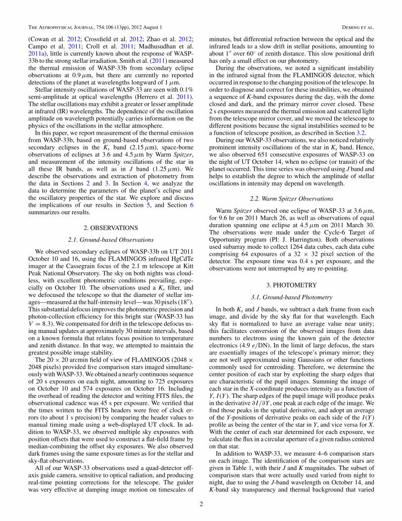
Many previous investigations have established that the intra-pixel effect is more dependent on the Y-coordinate than onthe X-coordinate, and it is stronger at 3.6 μm than at 4.5 μm(Knutson et al. 2009; Beerer et al. 2011; Deming et al. 2011a;Todorov et al. 2012). We see the intra-pixel effect in our 3.6 μmphotometry, and we corrected it using a quadratic fit to thephotometry as a function of the Y-coordinate of the image, witha linear term as a function of the X-coordinate (the variationwith X is weaker than for Y). However, we cannot detectany intra-pixel sensitivity variations in our 4.5 μm photometry.Plots of the measured intensity of the star versus both theX- and Y-coordinates of the image centroid are essentiallyscatter plots (not illustrated), with no significant trends. Pearsoncorrelation coefficients of intensity versus X- and Y-coordinateshave values near zero. We also calculated the Pearson correlationcoefficients for temporal subsets of the 4.5 μm data, chosenusing a moving boxcar window of various widths. We can findno significant correlations between our 4.5 μm photometry andspatial coordinates, during any time period. As an additionalcheck, we repeated our photometry using an alternative methodto determine the position of the star on the detector (center oflight). This method also failed to reveal correlation betweenposition and intensity. We therefore use our 4.5 μm photometryfor eclipse analysis without applying any spatial decorrelation.Note that we do see very small variations in the photometry at the40 minute period corresponding to the telescope oscillation (seeSection 4.4.2). We cannot rule out the possibility that the spatial-intensity correlation is being obscured by the stellar intensityoscillations.

In the case of the 3.6 μm photometry, we also used the spatialdecorrelation method described by Ballard et al. (2010). Thatweighting function method commonly uses a time threshold tozero-weight points that lie close in time to any given point. Whenthe only intrinsic temporal variation is an eclipse or transit, thetime threshold is straight forward to implement. However, whencontinuous stellar oscillations are part of the desired signal,the weighting function time threshold can be problematic. Weapplied a weighting function to the 3.6 μm photometry, usinga time threshold of zero, i.e., not excluding any points in thecalculated weights. Fitting to this alternative version of the3.6 μm photometry produced results that differed insignificantlyfrom our quoted results (0.34σ and 0.03σ differences in centralphase and eclipse depth, respectively). Our quoted results(see Section 4.4.2) are based on the polynomial decorrelationdescribed above because we believe that method is better suitedto the nature of these data.

After decorrelating (or not) the intra-pixel effect, we omitsome of the initial data for both Spitzer wavelengths. The 3.6 μmdata exhibit an initial transient drift in the image position,amounting to about 0.17 pixels, about four times as large asthe peak-to-peak variation caused by the 40 minute telescopeoscillation. This positional instability is accompanied by asimilar large transient effect in the photometry. We are familiarwith the nature of these large transient effects based on seeingthem in other Spitzer data. The relation between intensity andX, Y position is not the same during the transient as duringthe stable portion of the time series because the image tracesa different region of the pixel. Therefore, we omit the first83 minutes of the 3.6 μm data—this being the time for theposition of the image to stabilize. We see no obvious transient

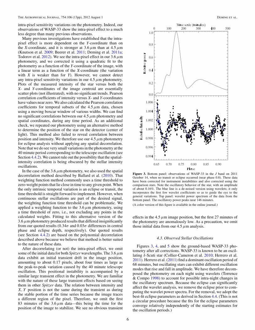
Figure 3. Bottom panel: observations of WASP-33 in the J band on 2011October 14, when no transit or eclipse occurred (near phase 0.8). These datahave been corrected for instrument instabilities and also corrected using thecomparison stars. Note the oscillatory behavior of the star, with an amplitudeof about 0.16%. The blue line is a de-noised version using wavelets; it onlyincorporates the first few wavelet coefficients so as to guide the eye to thegeneral variations. Top panel: wavelet power spectrum of the data from thebottom panel. The oscillatory power peaks near 146 minutes.

(A color version of this figure is available in the online journal.)

effects in the 4.5 μm image position, but the first 27 minutes ofthe photometry are anomalously low. As a precaution, we omitthose initial data from our 4.5 μm analysis.

4.3. Observed Stellar Oscillations

Figures 3, 4, and 5 show the ground-based WASP-33 pho-tometry after all corrections. WASP-33 is known to be an oscil-lating δ-Scuti star (Collier-Cameron et al. 2010; Herrero et al.2011). Herrero et al. (2011) find a dominant oscillation period of68 minutes, but oscillating stars can exhibit different oscillationmodes that rise and fall in amplitude. We have therefore decom-posed the photometry on each night using wavelets (Torrence& Compo 1998) to account for possible intra-night changes inthe oscillatory spectrum. Because the eclipse can significantlyaffect the wavelet analysis, we remove the eclipse prior to com-puting the wavelet power spectra. For the removal, we adopt thebest-fit eclipse parameters as derived in Section 4.4. (This is nota circular procedure because the fits for the eclipse parametersconverge relatively independently of the starting estimates forthe oscillation periods.)

6

The Astrophysical Journal, 754:106 (13pp), 2012 August 1 Deming et al.

Figure 4. Bottom panel: observations of WASP-33 in the Ks band on 2011October 10, spanning a secondary eclipse. These data have been corrected forinstrumental instabilities and also corrected using the comparison stars. Theblue line is a de-noised version using wavelets; it only incorporates the first fewwavelet coefficients so as to guide the eye to the general variations. Note the veryprominent stellar oscillation with period near 71 minutes. Top panel: waveletpower spectrum of the data from the bottom panel, showing the oscillation peakpower at 71 minutes.

(A color version of this figure is available in the online journal.)

Our results show the stellar oscillations very prominently,but (interestingly) to varying degrees. The J-band results areshown in Figure 3; the bottom panel shows the correctedphotometry and the overlaid blue line shows part of the waveletdecomposition—just the lowest order components to guide theeye to the general trend. (Note that we do not use the blue lineson Figures 3– 5 in our analysis, but we do use the results of thewavelet power spectra, shown in the upper panels.)

The power spectrum in Figure 3 peaks at 146 minutes(frequency 9.9 cycles day−1), close to twice the period of the68 minute oscillation (21.2 cycles day−1) seen by Herrero et al.(2011). There was no mention of this lower frequency mode inthe work of Herrero et al. (2011), but δ-Scuti stars are known toexhibit multiple periods of oscillation (Balona & Dziembowski2011), wherein the non-radial modes cluster around differentradial modes (e.g., n = 1, 2, 3, . . .; Breger et al. 2009). Hence,detection of a different mode frequency than Herrero et al.(2011) is not surprising. Figure 4 shows the results in similarformat for the Ks-band observations on October 10. In this casea very prominent oscillation is seen with a power spectral peakat 71 minutes (20.3 cycles day−1), in good agreement with

Figure 5. Bottom panel: observations of WASP-33 in the Ks band on 2011October 16, spanning a secondary eclipse. These data have been corrected forinstrumental instabilities and also corrected using the comparison stars. Theblue line is a de-noised version using wavelets; it only incorporates the first fewwavelet coefficients so as to guide the eye to the general variations. Top panel:wavelet power spectrum of the data from the bottom panel, showing oscillatorypower peaks at 54 and 126 minutes.

(A color version of this figure is available in the online journal.)

essentially the same oscillation period (68.56 minutes) that wasprominent in the results of Herrero et al. (2011). Note alsothat it can be clearly discerned in the photometry even priorto the correction using the comparison stars—see Figure 2.The amplitude of this oscillation—about 0.2% in flux—is abouttwice what was observed by Herrero et al. (2011) in the optical,and we discuss possible reasons for this difference in Section 5.

Figure 5 shows the analogous result for the Ks band observedon October 16. In this case we see two peaks in the powerspectrum at 54 and 126 minutes that are probably due to thestellar oscillations as seen on October 10 and 14. For eachnight, and also for the Spitzer data, we estimate the total stellaroscillation amplitude from the power present in the oscillatorycomponent of the Markov Chain Monte Carlo (MCMC) eclipsefit (see Section 4.4), and we tabulate those amplitudes in Table 2.All of these amplitudes are in reasonable agreement with the0.1% oscillation seen in the optical by Herrero et al. (2011),except in the Ks band where the amplitude is about twice asgreat, consistently on both October 10 and 16.

Variability in stellar oscillation amplitudes is sometimesobserved in δ-Scuti stars (e.g., Breger & Pamyatnykh 2006),

7

The Astrophysical Journal, 754:106 (13pp), 2012 August 1 Deming et al.

Table 2WASP-33 Stellar Infrared Oscillation Amplitudes and Timescales

UT Date (2011) Wavelength Oscillation Amplitude Timescale Observatory(μm) (s)

Mar 26 3.6 0.0013 68 minutes Warm Spitzer; Figure 8Mar 30 4.5 0.0013 68 minutes Warm Spitzer; Figure 7Oct 10 2.15 0.0023 71 minutes Kitt Peak 2 m; Figure 4Oct 14 1.25 0.0016 146 minutes Kitt Peak 2 m; Figure 3Oct 16 2.15 0.0021 54, 126 minutes Kitt Peak 2 m; Figure 5

Notes. Smith et al. (2011) found oscillation periods between 42 and 77 minutes, and Herrero et al. (2011) found a dominant period near 68 minutes.

but is not the most likely explanation for our results, becauseof our J-band data. Although the J band shows a prominentoscillation near phase 0.82 on Figure 3, quantitative calculationof the average amplitude over that entire night gives 0.16%(Table 2), only marginally higher than the optical value. Aclose-to-normal oscillation amplitude in J band, between thetwo nights of higher amplitude in Ks band, seems too muchof a coincidence to attribute to variability. While we cannotstrictly reject mode variability, we hypothesize that oscillationamplitude is associated with wavelength. We discuss possiblewavelength-related explanations in Section 5.2.

4.4. Eclipse of WASP-33b

4.4.1. Ks-band Eclipse

The eclipse of the planet is visible near phase 0.5 in the lowerpanels of Figures 4 and 5. No eclipse is seen in Figure 3, asexpected for that range of orbital phase. The stellar oscillationsare a very significant source of confusion as regards measuringthe properties of the eclipse. That confusion is mitigated bysufficiently long duration of our observed sequences (7.3 hr onOctober 10 and 5.4 hr on October 16) compared with the periodsof oscillation, and by the fact that the stellar oscillations will notbe in phase on the two nights, whereas the eclipse should repeatat the same orbital phase. In order to exploit the latter advantage,we combine the data for October 10 and 16 into one binned dataset, using a bin width of 0.001 in phase, and we fit models tothese binned data. Figure 6 shows the combined and binneddata, with best-fit eclipse plus oscillation curves overplotted.

To obtain the best-fit eclipse depth, we fit a combinationof eclipse curve plus two sinusoidal oscillations, using anMCMC method, with Gibbs sampling (Ford 2005). We fit tothe combined and binned data of Figure 6, in order to gainthe advantage of canceling the stellar oscillation as much aspossible. We generate four chains of 106 steps each, and wediscard the first 2 × 105 steps in each chain. We initialize theMCMC fit using sinusoids with periods of 68 and 146 minutes,guided by our wavelet power spectra in Figures 3– 5. TheMCMC fit is insensitive to the exact choice of initial periods. Aslong as the initial values contain one period in the ∼70 minuterange, and one period in the ∼140 minute range, the Markovchains rapidly converge to the best-fit values for that particulareclipse (this is also true for the Spitzer eclipses; Section 4.4.2).

In order to derive accurate MCMC posterior distributions,it is essential to re-scale the error bars to yield a best-reducedχ2 near unity. We find that errors about four times larger thanthe photon noise (for the binned data) are necessary to obtain abest-fit reduced χ2 of unity. Error re-scaling factors almost aslarge as three have been required in other investigations, evenfor very precise spectrophotometry (Bean et al. 2011). An evenlarger error re-scaling in our case is probably a consequence of

Figure 6. Top panel: eclipse of WASP-33b based on combining the Ks-bandobservations from October 10 and 16, and binning to a phase resolution of0.001. The blue line shows the result of fitting to the eclipse, and the sum of twooscillation modes, via Markov chains. Bottom panel: data from the top panelwith the oscillatory portion of the fit removed and compared with the best-fiteclipse (red line). The scatter per binned point is about 0.0012, indicated bythe inset point with error bars. The best-fit eclipse depth is 0.0027 ± 0.0002,but comparison of the two individual nights (not illustrated) indicates a greatererror in the depth (±0.0004, see Table 3).

(A color version of this figure is available in the online journal.)

the complexity of the stellar oscillation spectrum that is onlyapproximated using two oscillation periods. In other words,small amplitude residual oscillations may masquerade as noise.

We experimented with adding additional oscillation modes tothe fit, and indeed this does reduce the necessity for error re-scaling. However, we can only justify initializing the fit using thetwo periods that we can objectively identify in our wavelet powerspectra. Other modes, if present, cannot be resolved as clearoscillations in our ground-based data, instead they appear onlyas extra noise. We also verified that adding a third oscillation

8

The Astrophysical Journal, 754:106 (13pp), 2012 August 1 Deming et al.

Table 3WASP-33b Secondary Eclipse Depths, Time of Central Eclipse, and Orbital Phase

Wavelength Eclipse Depth Time as BJD(TDB) Phase Comment(μm)

2.15 0.0027 ± 0.0004 2455844.8156 ± 0.0040 0.4995 ± 0.0035 Average of October 10 and 16; Figure 63.6 0.0026 ± 0.0005 2455647.1978 ± 0.0001 0.50041 ± 0.00008 Warm Spitzer; Figure 74.5 0.0041 ± 0.0002 2455650.8584 ± 0.0005 0.5012 ± 0.0004 Warm Spitzer; Figure 8

Notes. For the ground-based eclipse at 2.15 μm the barycentric time of central eclipse is based on the average phase for both October 10 and 16, then converted to thecentral BJD value for the October 10 eclipse.

mode to our MCMC fit does not significantly alter the best-fiteclipse depth.

We vary nine parameters in the MCMC chains: an amplitude,period, and phase for two independent sinusoids, an eclipsedepth and central phase, and an additive constant. We generatethe eclipse curve using a new version of the Mandel & Agol(2002) methodology (see Deming et al. 2011b). We adoptsystem parameters that determine the shape and duration ofthe eclipse, from Collier-Cameron et al. (2010), except for theorbital period where we use the value from Smith et al. (2011).Observations of recent transits in the Czech Exoplanet TransitDatabase12 show that the original period from Collier-Cameronet al. (2010) is too short; the slightly longer period derived bySmith et al. (2011) is more consistent with recent transit timesin the Czech database.

The top panel of Figure 6 overplots the best-fit curve, in-cluding both the eclipse and oscillatory component. The lowerpanel removes the oscillatory component from the data andshows the comparison with the eclipse curve alone. Our best-fiteclipse has a depth of 0.0027 ± 0.0002, with central phase of0.4995 ± 0.0010. Those errors are implied by our MCMC pos-terior distributions. They include possible degeneracies betweenfitted parameters, but there can be external sources of error thanare not represented in the MCMC chains. The most obvioussource of such errors is the presence of unmodeled stellar os-cillation structure, as noted above. The most realistic check onthe errors is to fit each of the two independent nights separately,and compare the independent results. Those fits yield eclipsedepths of 0.0024 ± 0.0002 and 0.0033 ± 0.0004 for October 10and 16, respectively. The best-fit central phases for the separatenights are 0.502 ± 0.001 and 0.495 ± 0.001, so the differencebetween two independent nights exceeds the formal errors, es-pecially in the case of central phase. We adopt the best-fit valuesdetermined for the combined and binned data, but we assign theerrors based on the differences in the two independent nights.The difference between two independent values drawn from anormal error distribution is, on average, twice the error associ-ated with the average of those two values. So we estimate theerrors appropriate to our average Ks-band eclipse depth and cen-tral phase to be half the difference between the best-fit valuesfor the individual nights. Our best-fit eclipse depth and cen-tral phase is given in Table 3, together with the Spitzer eclipseresults.

4.4.2. The Eclipse in Warm Spitzer Bands

At both Spitzer wavelengths, we solve for the eclipsedepth and central phase also using an MCMC method, withGibbs sampling. We allow for an exponential baseline ramp(Harrington et al. 2007), because we find that a linear ramp is

12 http://var2.astro.cz/ETD/

inadequate. Indeed, detailed analysis of very high S/N Spitzer8 μm data (Agol et al. 2010) indicates that even a second ex-ponential term can be warranted. However, we use a single ex-ponential for two reasons. First, the single exponential rampalone is more complex than is normally required for thesespecific Spitzer bands (Knutson et al. 2009; Todorov et al.2012)—exponential ramps are normally only required at thelongest wavelength Spitzer bands. Second, our data do not attainsufficient S/N to justify the inclusion of a second exponentialterm.

As in the case of our ground-based data, we calculate waveletpower spectra at both Spitzer bands, and these are shown asthe upper panels of Figures 7 and 8. Like the ground-baseddata (perhaps a coincidence), we see two significant oscillatoryspectral peaks after removing the best-fit eclipse. Figure 7(3.6 μm) shows one of these peaks at 68 minutes. However,Figure 8 (4.5 μm) shows two peaks, 39 and 68 minutes. Theformer is likely to be associated with the Spitzer telescopepointing (Section 4.2), while the latter is clearly due to thestellar oscillation.

Our first MCMC fits at both Spitzer wavelengths vary 12 pa-rameters: two sinusoidal terms (each having amplitude, period,and phase), an eclipse of variable depth and central phase (i.e.,two parameters), the exponential ramp (three parameters), anda zero-point constant in intensity. We discard the first 20% ofeach 106-step Markov chain and locate the best-fit values fromthe minimum in χ2 (we keep track of χ2 during the evolution ofthe chain). Subtracting the best fit from the data, we find that theresiduals have a quasi-sinusoidal shape. These residuals repre-sent the unmodeled portion of the data. They can be due to rednoise in the data created by uncorrected instrumental effects,or by imperfect modeling of the stellar oscillations. Unlike thecase of our ground-based data, the Spitzer data have sufficientstability and S/N to define these small amplitude imperfectionsin the fit. Both the oscillating intensity of the star and (to a lesserextent) the subtlety of red noise caused by Spitzer’s improvedperformance require some new methodology in their analysis.We now introduce that new methodology.

Following the initial fit using a single MCMC chain of 106

steps, we re-fit by including an additional term to explicitlyaccount for the imperfections in the initial fit. We calculateresiduals for the first MCMC fit by subtracting that best fit fromthe data. We then approximate those residuals using a waveletdecomposition, using N coefficients for Morelet wavelets, andwe vary N in our subsequent analysis. For each choice of N,we multiply the wavelet decomposition of the residuals byan adjustable amplitude, and include that amplitude as a fitparameter in subsequent MCMC chains. In the limit whereN equals the number of data points, this procedure would betrivial, because the wavelet decomposition would reproducethe residuals exactly, and including those residuals in the fitwould simply be a fudge, wherein we arbitrarily subtract that

9

The Astrophysical Journal, 754:106 (13pp), 2012 August 1 Deming et al.

Figure 7. Middle panel: Spitzer observations of WASP-33 at 3.6 μm, spanninga secondary eclipse. The overplotted blue line is the best-fit solution from ourMCMC analysis, including structure defined by our wavelet analysis (see thetext). The dashed blue line omits the wavelet-defined structure and uses only thepure oscillatory portion, plus eclipse. Bottom panel: data from the middle panelwith the oscillatory plus wavelet portion removed, showing the best-fit eclipsecurve (red line). Top panel: wavelet power spectrum of the data points from themiddle panel. The peak near 68 minutes is due to oscillations of the star.

(A color version of this figure is available in the online journal.)

part of the data not accounted for by the model. In the realanalysis, this procedure is not trivial. With not-too-large N, thewavelet decomposition approximates only the major features ofthe residuals, not the point-to-point noise. Because the MCMCchain varies the amplitude of those major features, correlatingthe chained values of eclipse depth and phase with the amplitudeof the unmodeled features indicates the degree to which the best-fit eclipse depth and phase depend on unmodeled aspects of thedata. We determine the optimal N by examining the noise inthe final fits, requiring that it be close to, but not less than thephoton noise, and have no detectable red noise component. Thisdictates N = 9 for both our 3.6 and 4.5 μm data. Our finalvalues are based on four independent MCMC chains at N = 9,each having 106 steps, with the first 20% of each chain beingignored.

Using this procedure, we find that the Spitzer eclipse depthsand central phases are reasonably robust in the sense that theydo not vary greatly with N. This is especially true for the centralphase at 3.6 μm, and the eclipse depth at 4.5 μm. In those cases,the variation in eclipse depth and central phase, as we vary N,are consistent with the errors implied by the MCMC posterior

Figure 8. Middle panel: Spitzer observations of WASP-33 at 4.5 μm, spanninga secondary eclipse. The overplotted blue line is the best-fit solution from ourMCMC analysis, including structure defined by our wavelet analysis (see thetext). The dashed blue line omits the wavelet-defined structure and uses only thepure oscillatory portion, plus eclipse. Bottom panel: data from the middle panelwith the oscillatory plus wavelet portion removed, showing the best-fit eclipsecurve (red line). Top panel: wavelet power spectrum of the data from the middlepanel; the main peak near 68 minutes is due to oscillations of the star, and asecondary peak near 39 minutes is due to a pointing oscillation in the telescope.

(A color version of this figure is available in the online journal.)

distributions. However, for the converse set of parameters—the3.6 μm eclipse depth and 4.5 μm central phase—the agreementis not as good. In those cases, the differences in best-fit values aswe vary N are larger than the errors from the MCMC posteriordistributions, and we adopt the larger errors consistent with thefluctuations in the best-fit values as N varies.

The derived best-fit eclipse depths, central phases, and errorsare included in Table 3. We also extract the amplitude of thestellar oscillation in the Spitzer bands (see Table 2), based onthe total amplitude of the oscillatory portion of the MCMC fits,but with the 40 minute portion subtracted because we attributethat portion to the Spitzer observatory.

4.5. Models for the Atmosphere of WASP-33b

We interpret our observed planet–star flux contrast ofWASP-33b using plane-parallel models of the dayside at-mosphere of the planet. We use the atmospheric modelingand retrieval methodology of Madhusudhan & Seager (2009,2010). The model computes line-by-line radiative transfer for aplane-parallel atmosphere with the assumptions of hydrostatic

10

The Astrophysical Journal, 754:106 (13pp), 2012 August 1 Deming et al.

equilibrium and global energy balance. The composition andpressure–temperature (P-T) profile of the atmosphere are freeparameters in the model. Since there are as yet insufficient datato constrain abundances in WASP-33b, we adopt solar composi-tion for all elements except carbon, which we allow to increase inabundance, following Madhusudhan et al. (2011b). We explore avariety of temperature profiles, especially temperature profilesthat are consistent with nearly complete absorption of stellarirradiance. The models include all the major opacity sources ex-pected in hot hydrogen-dominated atmospheres, namely H2O,CO, CH4, CO2, TiO, and VO, and collision-induced absorption(CIA) due to H2–H2. Our molecular line lists are obtained fromFreedman et al. (2008), R. S. Freedman (2009, private com-munication), Rothman et al. (2005), Karkoschka & Tomasko(2010), and E. Karkoschka (2011, private communication). OurCIA opacities are obtained from Borysow et al. (1997) andBorysow (2002). A Kurucz model (Castelli & Kurucz 2004)is used for the stellar spectrum, and the stellar and planetaryparameters are adopted from Collier-Cameron et al. (2010).

5. RESULTS AND DISCUSSION

5.1. Stellar Oscillations

The first and most obvious result from our observationsis the existence and prominence of the stellar oscillations.WASP-33 was already known to exhibit oscillations, but theamplitude observed by Herrero et al. (2011) in the optical(Johnson R band) was about 0.001. Our results (Figures 3–5 andFigures 7– 8) show oscillation amplitudes in agreement with theoptical, except for Ks band where the amplitude is about twicethe optical value (2.15 μm, Table 2), as noted in Section 4.3.Because the largest difference with the optical amplitude is seenin our ground-based (Ks-band) data, we contemplated whetherthe difference could be attributed to errors in our ground-basedresult. An argument against that possibility is the prominence ofthe stellar oscillation in the raw photometry (e.g., upper panelof Figure 2). We therefore explore whether properties of thestellar atmosphere that may be unique to Ks band could causethe oscillations to have greater amplitude at that wavelength.

5.2. Stellar Atmospheric Effects

We here consider the possibility that the larger Ks-bandoscillation amplitude as compared with the optical is due tothe different height of formation for continuum radiation in thestellar atmosphere, in concert with height-dependent variationsin the mode amplitudes. Due to the increase in atomic hydrogenbound-free continuous opacity in the infrared, our Ks-bandobservations of WASP-33 sample a greater height in the stellaratmosphere than that observed by Herrero et al. (2011).

The upward propagation of a pressure-mode oscillation ina stellar atmosphere can in principle cause the mode ampli-tude to increase. As a propagating mode encounters lower massdensity, the wave velocity—and hence the temperature pertur-bation in the compression—increases. However, propagation isstrongly affected by the stratification of the stellar atmosphere(Marmolino & Severino 1991). Frequencies less than the acous-tic cutoff frequency will not propagate, and their velocity am-plitude decreases with height. To the extent that the temperatureamplitude scales with velocity, it too will decrease with heightfor non-propagating modes. The acoustic cutoff frequency isc/2H , where c is sound speed and H is the pressure scale height.We calculated the acoustic cutoff frequency and other parame-ters for WASP-33, using a Teff/ log(g)/[M/H] = 7500/4.5/0.0

model atmosphere from Castelli & Kurucz (2004). We find thatthe acoustic cutoff corresponds to an oscillatory period of about1 minute. The much longer period oscillations we observe forWASP-33 are therefore not propagating, and their amplitudesshould decay with height.

The dominant opacity due to atomic hydrogen (Menzel &Pekeris 1935) is higher at 2.15 μm versus the optical by afactor of about 1.6, translating to a height difference of about60 km. That is not sufficient to account for significant changesin the mode properties even for propagating modes and, asnoted above, these modes do not propagate. Moreover, if heightdependence of the stellar continuous spectrum were significantto our observed amplitudes, then we would expect even largeramplitudes in the Spitzer bands than at 2.15 μm, which are notobserved.

However, there is one unique feature of the Ks band that maywell be responsible for a higher oscillation mode amplitude.The Brackett-γ line at 2.165 μm is centered in the Ks bandpass.The strong opacity in that line for an A5V star could have alarge potential effect on oscillation amplitudes. The impact ofstrong oscillations in the line, when diluted over the broad Ksband, could potentially be calculated using techniques beyondthe scope of this paper (i.e., radiation hydrodynamics). A moredirect method would be to obtain infrared spectroscopy ofthe star and directly measure the oscillations in the infraredhydrogen lines.

5.3. Orbit of WASP-33b

Our measured times of central eclipse can in principle deter-mine e cos ω for the planet’s orbit (e.g., Knutson et al. 2009).Considering the 25 s of light travel time across the planet’s or-bit, we expect to find the eclipse at phase 0.50024 if the orbit iscircular. Weighting both our ground-based and Spitzer eclipses(Table 2) by the inverse of their formal variances, we find an av-erage eclipse phase of 0.50044±0.00008, totally dominated bythe 3.6 μm eclipse. Thus, we find that e cos ω—approximated asπ/2 times the phase offset from 0.5—is 0.0003 ± 0.00013. Thecentral phase measurement for these eclipses is complicated bythe stellar oscillations, so more-than-usual caution is needed inthe interpretation of the measured central phase. Moreover, ourvalue for e cos ω differs from zero by less than 3σ , so our resultsprovide little evidence for a non-circular orbit.

5.4. Atmosphere of WASP-33b

Figure 9 shows our result for the eclipse of WASP-33b incomparison to two models of its atmosphere, both of whichagree with the available measurements to date. One of thesemodels has a temperature inversion with solar composition, andone has a non-inverted atmospheric structure with a carbon-richcomposition (Madhusudhan et al. 2011b). Their temperatureprofiles are shown in the bottom panel of Figure 9, with the ap-proximate formation depths of the four bandpasses overplottedas points. The Ks bandpass is relatively devoid of strong molecu-lar absorption features, and probes the relatively deep planetaryatmosphere (pressure, P ∼ 0.6 bars), relatively independent ofthe composition of the atmosphere (asterisks on Figure 9). (The3.6 μm bandpass also peaks relatively deep in the atmosphere,but has significant contribution from higher altitudes, havingmore molecular absorption than the Ks band.) The large eclipsedepth we observe in Ks band (brightness temperature ≈3400 K)thus indicates a hot atmosphere at depth, and a high effectivetemperature for the planet. Both models illustrated in Figure 9

11

The Astrophysical Journal, 754:106 (13pp), 2012 August 1 Deming et al.

Figure 9. Top panel: comparison of our measured eclipse depths (red-orangepoints at 2.15, 3.6, and 4.5 μm, and including Smith et al. 2011 at 0.9 μm) withtwo models for the atmosphere of WASP-33b: the green line is a carbon-rich non-inverted model, and the violet line is a solar composition model with an invertedtemperature structure. The squares are the values expected by integratingthe planetary fluxes over the bandpasses. Bottom panel: pressure–temperatureprofiles for the models whose emergent spectra are shown in the top panel.The peaks of the contribution functions for each bandpass are plotted as pointson the pressure–temperature profiles. Squares are 0.9 μm, asterisks are 2.1 μm,triangles are 3.6 μm, and diamonds are 4.5 μm.

(A color version of this figure is available in the online journal.)

have hot lower atmospheres (both above 2500 K) and both haveinefficient longitudinal energy re-distribution. These models areconsistent with the observed tendency for the most strongly ir-radiated planets to exhibit the least longitudinal re-distributionof heat (Cowan & Agol 2011; Perna et al. 2012). We find thatthese very hot models are necessary to reproduce our results aswell as the result of Smith et al. (2011), and we conclude thatWASP-33 strengthens the Cowan & Agol (2011) result.

The two models we show are representative of a larger set ofsolutions that explain the data with and without thermal inver-sions. Given that there are 10 model parameters (Madhusudhan& Seager 2009, 2010) and only four data points, it is not possi-ble to derive a unique model fit to the data. We ran large MCMCchains (of ∼106 models) with and without thermal inversions,and identified regions of composition space in each case that arefavored by the data (Madhusudhan & Seager 2010).

Both models on Figure 9 are unusual as compared with, for ex-ample, the well-observed archetype HD 189733b (Charbonneauet al. 2008). One model in Figure 9 adopts solar composition but

with an inverted temperature structure (temperature rising withheight), while the other model has temperature declining withheight, but requires a carbon-rich composition. We integrate thefluxes of each planetary model, and the Kurucz model stellaratmosphere, over the observational bandpasses, and ratio thoseintegrals. These band-integrated points are shown as squaresin Figure 9. The χ2 values for the models as compared to allfour observed points (our three measurements, plus Smith et al.2011) are 7.9 for the inverted solar-composition model and 2.8for the non-inverted carbon-rich model. The Ks-band point at2.15 μm favors the non-inverted model. Although the differenceis not sufficiently significant to rule out the inverted model atthis time, additional eclipse observations in the Ks band wouldbe helpful for ruling out this type of atmospheric structure.

In our population of models with thermal inversions, severalmodels with slightly different inverted temperature structurefit the data almost equally well. However, none of them fitthe K-band point to within the 1σ errors while also fitting theremaining points. The Figure 9 model is the best among this setof inverted models.

In our models without thermal inversions, the best-fit modelrequires a carbon-rich composition (i.e., C/O � 1). However, atthe 2σ level of significance per wavelength point, several solarcomposition models (not illustrated) provide an acceptable fit tothe data. So, although the carbon-rich composition is favored, asolar abundance composition cannot be absolutely ruled out.

Our results illustrate the limitations of eclipse photometryin broad bands, especially for challenging cases like planetsorbiting oscillating stars. Once we admit the possibility of non-solar compositions (because we are largely ignorant of trueexoplanetary compositions), the range of models that can fitbroadband photometry can be large, in this case extending toinverted and non-inverted models with drastically different tem-perature structure. The degeneracy is exacerbated by the rela-tively small range of atmospheric pressures probed by the fourbandpasses we analyze (points on the bottom panel o Figure 9).Fortunately, future observations can break this degeneracy us-ing Hubble Space Telescope/WFC3 spectroscopy near 1.4 μm(Berta et al. 2012). The water band near 1.4 μm is sufficientlystrong that eclipse observations with the Hubble WFC3 grismshould be feasible. Although water absorption in the carbon-rich model is suppressed by C/O > 1, the water emission in thesolar-composition inverted model is predicted to be significant,readily detectable near 1.4 μm (see Figure 9). Moreover, spec-troscopic techniques can potentially probe a larger depth rangein exoplanetary atmospheres than does photometry because thecores of resolved spectral features have strong opacities. Ourresults therefore illustrate the complementary value of acquir-ing both broadband and spectroscopic observations of transitingexoplanets at secondary eclipse.

6. SUMMARY

We have analyzed ground-based and Spitzer infrared obser-vations of the strongly irradiated exoplanet WASP-33b. Ourobservations span the time of secondary eclipse in Ks band andthe Warm Spitzer bands at 3.6 and 4.5 μm. We also observed thesystem for one ground-based night out of eclipse in the J band(1.25 μm). Oscillations of the δ-Scuti host star are prominentin our data, with a semi-amplitude (0.1%) about the same asin the optical. One exception is the Ks band, where we find anoscillation amplitude about twice as large as seen in the optical.Neither temporal variability nor the variation of stellar continu-ous opacity with wavelength is likely to account for our Ks-band

12

The Astrophysical Journal, 754:106 (13pp), 2012 August 1 Deming et al.

result. We speculate that the greater amplitude in Ks band maybe related to the presence of the Brackett-γ line in the bandpass.

We measure two Ks-band eclipses, and we base our errorsfor the eclipse depth and central phase on the differencebetween the two independent measurements. In the case ofthe Spitzer bands, we measure one eclipse in each band. OurSpitzer observations exhibit a relatively low level of intra-pixelsensitivity variation as compared with previous observationsof other exoplanets. However, all of our observed eclipses areoverlaid by the ubiquitous stellar oscillations. We adopt aneclipse model comprised of the eclipse shape, plus two sinusoidsto account for the stellar oscillations. We fit the model to thephotometry using an MCMC method. The Spitzer photometryis of sufficient quality that we are able to implement a wavelet-based technique to define fluctuations in the data that are notaccounted for by our fitting procedure. Including that structureas a parameter in subsequent MCMC fits, we thereby explorehow the eclipse depth and central phase vary as a function ofthe amplitude of the unmodeled structure. The derived eclipsedepth and central phase of the Spitzer eclipses are not stronglysensitive to unmodeled structure in the light curves, but thisprocedure does allow a realistic evaluation of the errors.

Using the million-model approach pioneered byMadhusudhan & Seager (2009) and Madhusudhan & Seager(2010), we explore the range of atmospheric temperature struc-tures and compositions that are consistent with our eclipse ob-servations, plus the 0.9 μm eclipse observed by Smith et al.(2011). We find two possible atmospheric models. One has aninverted temperature structure and a solar composition, and thesecond has a non-inverted temperature structure with a carbon-rich composition. We point out the value of infrared eclipsespectroscopy using moderate resolving power to detect (for ex-ample) the water band near 1.4 μm. Spectroscopic detection ofwater emission or absorption at eclipse would break the degener-acy between the two possible models. Although the temperaturestructure of WASP-33b is currently ambiguous, both models re-emit a large fraction of incident stellar irradiation from their daysides, strengthening the hypothesis of Cowan & Agol (2011)that the most strongly irradiated planets circulate energy to theirnight sides with low efficiency.

REFERENCES

Agol, E., Cowan, N. B., Knutson, H. A., et al. 2010, ApJ, 721, 1861Ballard, S., Charbonneau, D., Deming, D., et al. 2010, PASP, 122, 1341Balona, L. A., & Dziembowski, W. A. 2011, MNRAS, 417, 591Bean, J. L., Desert, J.-M., Kabath, P., et al. 2011, ApJ, 743, 92Beerer, I. M., Knutson, H. A., Burrows, A., et al. 2011, ApJ, 727, 23Berta, Z. K., Charbonneau, D., Desert, J.-M., et al. 2012, ApJ, 747, 35Borysow, A. 2002, A&A, 390, 779Borysow, A., Jorgensen, U. G., & Zheng, C. 1997, A&A, 324, 185

Breger, M., Lenz, P., & Pamyatnykh, A. A. 2009, MNRAS, 396, 291Breger, M., & Pamyatnykh, A. A. 2006, MNRAS, 368, 571Burrows, A., Hubeny, I., Budaj, J., Knutson, H. A., & Charbonneau, D.

2007, ApJ, 668, L171Campo, C. J., Harrington, J., Hardy, R. A., et al. 2011, ApJ, 727, 125Carey, S. J., Surace, J. A., Glaccum, W. J., et al. 2010, Proc. SPIE, 7731, 77310NCastelli, F., & Kurucz, R. L. 2004, in IAU Symp. 210, Modelling of Stellar

Atmospheres, ed. N. Piskunov, W. W. Weis, & D. F. Gray (San Francisco,CA: ASP), A20

Charbonneau, D., Knutson, H. A., Barman, T., et al. 2008, ApJ, 686, 1341Collier-Cameron, A., Guenther, E., Smalley, B., et al. 2011, MNRAS, 407,

507Cowan, N. B., & Agol, E. 2011, ApJ, 729, 54Cowan, N. B., Machalek, P., Croll, B., et al. 2012, ApJ, 747, 82Croll, B., Lafreniere, D., Albert, L., et al. 2011, AJ, 141, 30Crossfield, I., Hansen, B. M. S., & Barman, T. 2012, ApJ, 746, 46Deming, D., Knutson, H., Agol, E., et al. 2011a, ApJ, 726, 95Deming, D., Sada, P. V., Jackson, B., et al. 2011b, ApJ, 740, 33Demory, B.-O., Gillon, M., Deming, D., et al. 2011, A&A, 533, A114Desert, J.-M., Charbonneau, D., Fortney, J. J., et al. 2011, ApJS, 197, 11Ford, E. B. 2005, AJ, 129, 1706Fortney, J. J., Lodders, K., Marley, M. S., & Freedman, R. S. 2008, ApJ, 678,

1419Freedman, R. S., Marley, M. S., & Lodders, K. 2008, ApJS, 174, 504Guillot, T., Burrows, A., Hubbard, W. B., Lunine, J. I., & Saumon, D. 1996, ApJ,

459, L35Harrington, J., Luszcz, S., Seager, S., Deming, D., & Richardson, L. J.

2007, Nature, 447, 691Hebrard, G., Desert, J.-M., Dıaz, R. F., et al. 2010, A&A, 516, A95Herrero, E., Morales, J. C., Ribas, I., & Naves, R. 2011, A&A, 526, L10Karkoschka, E., & Tomasko, M. G. 2010, Icarus, 205, 674Knutson, H. A., Charbonneau, D., Allen, L. E., Burrows, A., & Megeath, S. T.

2008, ApJ, 673, 526Knutson, H. A., Charbonneau, D., Burrows, A., O’Donovan, F. T., & Mandushev,

G. 2009, ApJ, 691, 866Knutson, H. A., Howard, A. W., & Isaacson, H. 2010, ApJ, 720, 1569Madhusudhan, N., Harrington, J., Stevenson, K. B., et al. 2011a, Nature, 469,

64Madhusudhan, N., Mousis, O., Johnson, T. V., & Lunine, J. I. 2011b, ApJ, 743,

191Madhusudhan, N., & Seager, S. 2009, ApJ, 707, 24Madhusudhan, N., & Seager, S. 2010, ApJ, 725, 261Mandel, K., & Agol, E. 2002, ApJ, 580, L171Marmolino, C., & Severino, G. 1991, A&A, 242, 271Menzel, D. H., & Pekeris, C. L. 1935, MNRAS, 96, 77Perna, R., Heng, K., & Pont, F. 2012, ApJ, 751, 59Rothman, L. S., Jacquemart, D., Barbe, A., et al. 2005, J. Quant. Spectrosc.

Radiat. Transfer, 96, 139Seager, S., & Deming, D. 2010, ARA&A, 48, 631Showman, A. P., Cooper, C. S., Fortney, J. J., & Marley, M. S. 2008, ApJ, 682,

559Smith, A. M. S., Anderson, D. R., Skillen, I., Collier-Cameron, A., & Smalley,

B. 2011, MNRAS, 416, 2096Spiegel, D. S., Silverio, K., & Burrows, A. 2009, ApJ, 699, 1487Todorov, K. O., Deming, D., Knutson, H. A., et al. 2012, ApJ, 746, 111Torrence, C., & Compo, G. P. 1998, Bull. Am. Meteorol. Soc., 79, 61Zahnle, K., Marley, M. S., Freedman, R. S., Lodders, K., & Fortney, J. J.

2009, ApJ, 701, L20Zhao, M., Monnier, J. D., Swain, M. R., Barman, T., & Hinkley, S. 2012, ApJ,

744, 122

13