infrared cooling rate calculations in operational

JOURNAL OF GEOPHYSICAL RESEARCH, VOL. 96, NO. D5, PAGES 9105-9120, MAY 20, 1991

Infrared Cooling Rate Calculations in Operational General Circulation Models:

Comparisons with Benchmark Computations

S. B. FELS, •,2 J. T. KIEHL, 3 A. A. LACIS, 4 AND M.D. SCHWARZKOPF 2

As part of the Intercomparison of Radiation Codes in Climate Models (ICRCCM) project, careful comparisons of the performance of a large number of radiation codes were carried out, and the results compared with those of benchmark calculations. In this paper, we document the performance of a number of parameterized models which have been heavily used in climate and numerical prediction research at three institutions: Geophysical Fluid Dynamics Laboratory (GFDL), National Center for Atmospheric Research (NCAR), and Goddard Institute for Space Studies (GISS).

1. INTRODUCTION

One of the important goals of the World Meteorological Organization (WMO)-sponsored Intercomparison of Radi- ation Codes in Climate Models (ICRCCM) project was the careful documentation of the performance of radiation codes which have been used in operational climate and numerical weather prediction models. To this end, exten- sive statistical summaries have been compiled which give a pr6cis of the most important fluxes calculated by various models for a large number of standard ICRCCM cases. The article by Ellingson et al. [this issue] discusses some of these results. In addition to fluxes at the top and bottom of the atmosphere, however, the infrared cooling rates themselves play an important part in determining the chmatology of the model atmosphere. It has been suggested, for example, that the "cold bias" observed in the upper troposphere of a number of climate models might be due to deficiencies in the treatment of radiative cooling there. In addition to such direct chmatological effects, there is some evidence [Ramanathan et al., 1983] that subtle changes in the treatment of radiative transfer can also have important effects on the model dynamics.

It is therefore desirable to have available a rather

detailed discussion of the cooling rates as well as of the fluxes calculated by radiative models used in a number of operational general circulation models, together with a brief description of their construction and shortcomings. It is the purpose of this paper to provide these.

Radiation models discussed in this study have been used over a period of time in general circulation models (GCMs), and there exists a body of hterature describing applications of these GCMs to diverse climate problems. We are chiefly interested in documenting the behavior, even if less accurate, of older "production" GCMs including these radiative models, rather than in evaluating the performance of more detailed "off-fine" models or newer models, which are currently under development.

1Deceased October 22, 1989. 2Geophysical Fluid Dynamics Laboratory, Princeton, New

Jersey. 3National Center for Atmospheric Research, Boulder, Colorado. 4NASA Goddard Institute for Space Studies, New York.

Copyright 1991 by the American Geophysical Union.

Paper number 91JD00516. 0148-0227/91/91JD-00516505.00

The models to be described are fisted in Table 1, along with their chief architects and period of active use. It is interesting to notice that in several instances, more than one distinct radiation code has been in use at a given institution. We believe that the models discussed cover

a significant fraction of the GCM climate and numerical weather prediction literature of the past decade. .

It is important to recognize that very often radiative algorithms undergo revision during their working fifetime. While this is often due to a desire to include new physics or to increase computational speed, it is also occasionally due to the discovery of a code error. In the descriptions which follow, a conscientious effort has been made to discuss such changes if they make a significant difference in the performance of the code.

The organization of the paper is extremely simple. In the next section, we briefly describe the standard ICRCCM cases that all of the models use. In subsequent sections, the performance of each of the models is documented.

We have tried to keep the description uniform across the various models. Within each model section, the level structure is first summarized, and a very brief description of the particular model given, along with a short summary of the major publications in which it has appeared. The cooling rate and flux results are then presented (on the actual model levels), along with the corresponding values obtained from line-by-fine benchmark calculations carried out in the course of the ICRCCM study. Finally, there is a brief discussion of these results.

2. DESCRIPTION OF ICRCCM CASES AND THE

LINE-BY-LINE MODEL

From the original 37 standard cases of the ICRCCM protocol for clear-sky longwave calculations, we shall present coohug rates and fluxes for three: 25, 27, and 33 (tropical (T), mid-latitude summer (MLS), and subarctic winter (SAW), respectively). The temperature, water vapor, and ozone mixing ratio profiles for these cases are given by McClatchey et al. [1972]. Carbon dioxide is assumed to be uniformly mixed at 300 ppmv.

In addition to these three cases, we shall also present selected flux difference results using cases 26, 28, and 36. These are the same soundings as the previous three, but with 600 ppmv CO2. In most cases, it is the change in the net flux at the tropopause that will be of greatest interest, since it is most directly related to the change in tropospheric temperature in GCMs.

9105

9106 FELS ET AL.: OPERATIONAL MODEL COMPARISON

TABLE 1. Description of Models Employed in Comparison

Institute Model Chief Architects Period of Use

GFDL I Manab e 1970-1984 II and 1984-1986

III Stone 1986-present

I Fels and 1975-present II Schwarzkopf 1986-present

N CAR CCM0 Ramanathan 1983-1987

CCM1 Kiehl, Hamanathan, and Brieg]eb 1987-present

GISS Model II Lacis and Oinas 1983-present

The benchmark calculations were performed using the Geophysical Fluid Dynamics Laboratory (GFDL) line-by- line (LBL) model, which is a distant descendant of the code described by Drayson [1973]. Full details of these LBL calculations are described by Schwarzkopf and Fels [this issue]. The calculations, which fully resolve even the centers of Voigt lines, include a frequency range extending from 0 to either 2200 or 3000 cm-1. In making comparisons with the parameterired calculations, the LBL values are given over the same frequency range as that used in the parameterizations. Cooling rate comparisons are, in any case, quite insensitive to the choice of the upper bound, provided the water vapor rotation band is fully included. Spectral data are taken from the 1980 Air Force Geophysics Laboratory (AFGL) compilation [Rothman, 1981]. Water vapor and ozone line absorption profiles are cut off at 10 cm -1 and carbon dioxide lines at 3 cm -1 The water , ß

vapor continuum is included with coefficients taken from Roberts et al. [1976]. The vertical grid has 123 levels between the ground and about 90 km. Temperature profiles for this grid are generated using the algorithm described by Fels [1986], while the water vapor and ozone mixing ratios are obtained by interpolation from the tables in McClatchey et al. [1972]. Further details on the vertical' grid and on the derivation of the vertical profiles are found in Appendix A of Schwarzkopf and Fels [this issue].

In the following sections, these LBL results are compared with those obtained with the parameterired models included in Table 1. In general, the errors made by the GCM calculations are due to (1) the lack of spectral resolution (and to other physical approximations), and (2)the lack of vertical resolution. In almost all of the results

to be discussed, the errors include contributions from both sources. To evaluate the significance of errors in the parameterired models due to vertical resolution, we include, in section 6, a discussion of the effect of increased vertical resolution on the National Center for Atmospheric Research Community Climate Model, version 1 (NCAR CCM1) model results; a similar discussion on the Fels- Schwarzkopf model is found in Schwarzkopf and Fels [this issue]. Although differences are observed in fluxes at the tropopause and the top, and in upper tropospheric cooling rates, the overall conclusions of this paper are not significantly affected.

Cooling rate results from the LBL model are presented as continuous solid lines in all figures, a representation consistent with the high vertical resolution employed. Results from parameterired models are displayed as averages over the coarse vertical layers used in these models.

3. GFDL MODEL RESULTS

(MANABE-STONE, VERSIONS I, II, AND III)

Model Description and Usage The Manabe-Stone algorithm has been the standard

radiative transfer module used for chinate modehng at GFDL since 1970. It is primarily a tropospheric model; most research with it employs a nine-level •r-vertical coordinate grid, with temperatures, mixing ratios, and coohng rates carried at sigma levels of 0.025, 0.095, 0.205, 0.350, 0.515, 0.680, 0.830, 0.940, and 0.990. Water vapor is treated using the 19 band random-model formulation of Rodgers and Walshaw [1966]. All of the models discussed in this section use the spectral data given in that paper. Carbon dioxide transmission functions are calculated by interpolation from tables of absorptivities whose arguments are pressure, absorber amount and temperature. The tabulated values have been obtained from LBL calculations

for homogeneous paths performed by R. Drayson. The ozone 9.6-/•m band is included by use of the one-band Malkmus formulation of Rodgers [1968]. The frequency range extends from 0 to 2200 cm-1.

There have been a number of changes during the time in which the code has been in use. The most important of these is the replacement of the p-type water continuum (version I) of Rodgers and Walshaw [19½½1 by the e-type continuum of Bignell [1970]. This modification was made in 1984, but due to a code error, the strength of the continuum was underestimated by 62% (version II). Papers that use this code have been indicated below by an asterisk. In 1985, this error was corrected and continuum coefficients were taken from Roberts et al. [1976] (version III); papers incorporating this correction are shown with a double asterisk. A detailed description of the original model construction is given by Stone and Manabe [1968].

This radiation code has been used in all of the chmate

simulation and increased carbon dioxide sensitivity studies carried out at GFDL by Manabe and collaborators since 1970. These include the effect of increased CO2 in an annually averaged GCM [Manabe and Wetheraid, 1975], in a seasonal model [ Wetheraid and Manabe, 1981; Manabe and Wetheraid, 1987'], in a global model with a mixed layer [Manabe and Stouffer, 1979, 1980], and in a combined ocean-atmosphere model [Bryan et al., 1982, 1988'*]. In view of the emphasis on this problem, we shall pay special attention in our discussion of the results to those that involve sensitivity to doubled carbon dioxide. In addition, the code has been used in studies of interannual chmate variability, E1 Nifio-Southern Oscillation (ENSO), and of paleoclimate [Manabe and Broccoli, 1985; Broccoli and Manabe, 1987].

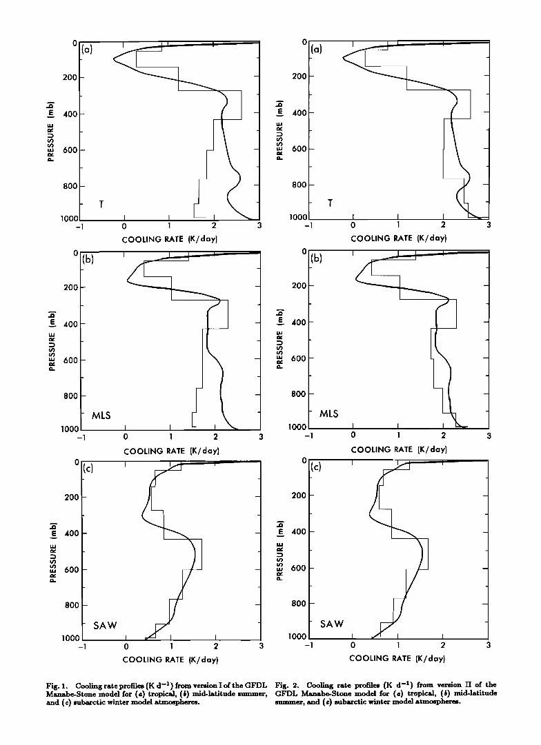
Cooling Rate Results Cooling rates computed using the parameterized and

LBL algorithms for the T, MLS, and SAW profiles are displayed in Figures l a-lc (for version I), in Figures 2a-2c (for version II), and in Figures 3a-3c (for version III). Comparison of the results for version I, which had a simple p-type continuum, with those of the other versions indicates clearly that the crude treatment of the continuum leads to a significant underestimate of the lower tropospheric coohng rates in the water-rich T and MLS cases. The excessive coohng near 350 mbar has been explained by Ramanathan and Downey [1986] as being due to the use

0 a)

200 400

600

800 1000 I I I

-1 0 1 2 3

COOLING RATE (K/day)

200

400

"' 600

8OO

(b)

- MLS

lOOO I I -1 o 1

I

2

(c)

200 -

_

_

_

800 -

• SAW

lOOO

E 400

•u 600

COOLING RATE (K/dayJ

I I

o 1 2


200

400

6oo

8OO

lOOO

200

400

600

8OO

lOOO

(a) I

I I i _ o 1 2 3


(b)

MLS

I

øic) 200 t 400

600

8OO

lOOO

I(

o 1 2


- SAW

I I 0 1 2 3


Fig. 1. Cooling rate profiles (K d -•) from version I of the GFDL Fig. 2. Cooling rate profiles (K d -•) from version II of the Manabe-Stone model for (a) tropical, (b) mid-latitude summer, GFDL Manabe-Stone model for (a) tropical, (b) mid-latitude and (c) subarctic winter model atmospheres. summer, and (c) subarctic winter model atmospheres.


o

200

4OO

6OO

800

1000

0

200 -

_

_..E 400-

_

"' 600 -

_

800 -

_

lOOO -1

i i

I I o 1 2

COOLING RATE (K/dayl

J _

I i

MLS

I I 0 1 2


200

•'E 400

600

8OO

1000 -1 o 1 2 3


Fig. 3. Cooling rate profiles (K d -1) from version III of the GFDL Manabe-Stone model for (a) tropical, (J•) mid-latitude stunmer, and (c) subarctic winter model atmospheres.

of overly broad spectral bands in Rodgers and Walshaw's water vapor random model.

Introduction of the Bignell continuum in version II leads to a substantial reduction in the undercooling of the lower troposphere longwave cooling rates. Correction of the code errors in the Bignell continuum formulation (version III) appears to almost entirely eliminate the undercooling. The only remaining error of importance is that near 350 mbar.•

Flux Results

Table 2 presents fluxes at the surface, tropopause, and top of the atmosphere for each of the three versions of the Manabe-Stone model for the three standard soundings, along with the LBL results. In addition, the sensitivity of the various fluxes to a doubling of CO2 is given.

TABLE 2. Comparison of LBL Fluxes With Manabe-Stone GFDL Models

rnet(1X) Fne'(1X)-Fne'(2X)

Model Model

LBL I II III LBL I II III

T

MLS SAW

T

MLS SAW

T MLS

SAW

Top 298.3 300.9 298.3 296.2 3.3 3.8 3.6 3.5

289.0 289.0 288.4 286.7 3.0 3.5 3.3 3.2

203.0 201.0 201.1 200.9 1.7 2.1 2.1 2.1

Tropopa us e 288.1 294.8 292.5 290.5 5.8 5.7 5.5 5.3

272.8 271.7 271.4 269.7 5.6 5.6 5.5 5.3

178.2 176.5 176.6 176.4 3.6 3.8 3.8 3.8

Surface 66.5 102.4 70.0 64.0 1.3 2.0 0.5 0.2

79.1 103.5 84.3 76.9 1.8 2.2 1.0 0.4

82.9 81.8 82.1 79.1 2.9 2.7 2.6 2.5

The tropopause is at 93.7 mbar for the T case; 179 mbar for the MLS case; 282.9 mbar for the SAW case.

At the top of the atmosphere and at the tropopause, the three parameterized models obtain fluxes for the 300 ppmv CO2 cases with typical errors of a few W m-2; in view of the other uncertainties associated with climate models, this must be considered quite adequate. In addition, the changes in the fluxes produced by a doubling of CO2 are generally accurate to within 20%. It is significant that the parameterized models (especially version III) underestimate the meridional gradient in the forcing due to doubled CO2 by up to 30%. A possible explanation is the neglect of the 10-/•m bands of CO2. Line-by-line results indicate that ~0.3 W m -2 of the sensitivity to doubled carbon dioxide for the T and MLS cases at the tropopause is due to these bands. At high latitudes, these lines are unimportant, due to the strong temperature dependence of this complex.

The situation at the surface is quite different and rather puzzling. As discussed above, the earliest version of the model has very large lower tropospheric cooling rate errors in the tropics and mid-latitudes; these are reflected in the significant surface flux errors, which are on the order of 30 W m -2. This underestimate of the downward flux at the surface presumably results in a compensating underestimate of the upward sensible and latent heat fluxes from the surface into the atmosphere. In the two later versions of the model, this problem is largely eliminated, since the e-type continuum is now included.

FELS ET AL.: OPEI•ATIONAL MODEL COMPAI•ISON 9109

Remarkably enough, however, the surface flux sensitivities to doubled C02 show a very different picture. Here, it is the original p-type model which most nearly reproduces the LBL results, while the newest model does a very poor job. Closer investigation reveals that the main source of error lies in the omission of the 10-/•m complex from any of the parameterized models. LBL calculations indicate that ~0.7 W m -2 of the CO2 flux sensitivity is due to these lines in the tropical case, and ~0.6 W m -2 in the MLS case. Thus, the apparently good results using version I are fortuitous, and due to an overestimate of the surface flux change due to the 15-/•m band complex. Although it is certainly true that changes in the surface flux may not be of the greatest importance for many climate model applications [Kiehl and Ramanathan, 1982], complicated results such as these may be of importance for the interpretation of changes in the surface energy budget.

4. GFDL MODEL RESULTS

(FELS-SCHWARZKOPF VERSIONS I AND II) Model Description and Usage

The Fels-Schwarzkopf radiation code has been employed operationally at GFDL in the troposphere-stratosphere- mesosphere GCM ("SKYHI") and in a numerical weather prediction model used by Miyakoda and collaborators. The radiation algorithm is designed to be usable from the surface to about 75 kin. Water vapor is treated by means of the simplified exchange approximation of Fels and Schwarzkopf [1975], carbon dioxide by precomputation of transmission functions as described in Fels and Schwarzkopf[1981], and ozone by the one-band random Malkmus model of Rodgers [1968]. The latter is crudely corrected for Doppler effects using the fast approximate method given by Fels [1979]. In the original (1975) formulation of the algorithm (version I), a p-type water vapor continuum with a frequency- dependent absorption coefficient is included in the 800 to 1200 cm -1 frequency range. In other implementations of the algorithm, an e-type water continuum is included in the region from 560 to 1200 cm -1 with the absorption coefficients being obtained from Roberts et al. [1976]. In this version, water vapor spectral data is derived from the 1982 AGFL compilation [Rothman et al., 1983]. The frequency range extends from 0 to 2200 cm-1.

Version I of the Fels-Schwarzkopf radiation code has been implemented in the "SKYHI" GCM at GFDL. This model has 40 levels extending from the surface to about 80 km. In view of the large number of levels, we refer the reader to Fels et al. [1980] for a description of the vertical structure. In the interest of maintaining a uniform radiation algorithm over a very long integration, this implementation was never changed in the "SKYHI" results described below. The "SKYHI" GCM has been used in a

large number of simulation and sensitivity studies, including Fels et al. [1980] (effect of altered CO2 and 03 levels on the middle atmosphere), Mahlman and Umscheid [1984, 1987] (simulated sudden warming, ultra-high resolution dynamics), Hayashi et al. [1984] (simulation of tropical waves), Miyahara et al. [1986] (effect of resolved gravity waves on planetary waves), and Hamilton and Mahlman [1988] (dynamics of simulated semiannual oscillation).

The second implementation (version II) of the Fels- Schwarzkopf algorithm is used in the numerical prediction models employed at GFDL and at several operational

meteorological centers. This version was used in the model employed to produce the GFDL First Garp Global Exper- iment (FGGE) level 2b data set [Miyahara et al., 1986]. An 18-level version is currently used in the operational medium range forecast (MRF) model at the National Me- teorological Center (NMC), and by the Australian Bureau of Meteorology Research Centre.

Cooling Rate Results We begin with the results from version I, used in the

"SKYHI" model. In view of the large altitude range covered, we shall present figures both in p as the vertical coordinate and in log p; the former emphasizes the troposphere and the latter the middle atmosphere.

Figures 4a and 4d show results for the tropical case. We see first of all that the algorithm does very well in the lower troposphere (below ~850 mbar), with errors less than 0.1 K d -z. This is quite remarkable in view of the fact that this model does not have an e-type continuum. One reason for this agreement is that the frequency-dependent p-type continuum coefficients used in this model were crudely based on the actual atmospheric observations of Vigroux [1959] and Saiedy [1960] as summarized by Goody [1964]. In the 500-800 mbar range, the model is seen to undercool by ~0.3 K d-1. A detailed investigation of the errors of the parameterized GFDL model in various frequency ranges is reported by Schwarzkopf and Fels [this issue]. From those results it appears that the undercooling results from a number of factors, principally the neglect of continuum absorption from 400 to 800 cm -• (especially in the 500-600 mbar range), and the use of wide spectral intervals in the precomputation of emissivities.

Above 500 mbar, the algorithm gives results quite similar to those of the various versions of the Manabe-

Stone algorithm discussed by section 3. This is no accident, since, as described by Fels and Schwarzkopf [1975], the present method was designed to be a fast and accurate approximation to Rodgers and Walshaw [1966]. In particular, the 0.2 K d -z overcooling at ~300 mbar is due to the use of overly broad frequency intervals in the water vapor random model. This excessive cooling is expected to produce an upper tropospheric cold bias in the model; on the basis of unpublished experiments performed by Schwarzkopf and Fels, this might account for about 2 K of the observed 8 K bias.

In the tropical stratosphere, the version I algorithm generally gives very good results, although undercooling is observed in the lower stratosphere, due to problems in the treatment of the 9.6-/•m 03 bands. This seemingly small error (about 0.1-0.2 K d -1) may lead to errors of the equilibrated temperature near 50 mbar of as much as 5-10 K, owing to the large radiative relaxation times in this region. More important, it makes attempts to use this particular model to diagnose vertical motion in this region rather suspect. The large error at the stratopause, which leads to an underestimate in the equilibrated temperature of ~5 K, is due to the neglect of several minor bands of CO2 and 03, as well as to poor treatment of Voigt effects. Errors in the treatment of the stratosphere are discussed in more detail in the article by Schwarzkopf and Fels [this issue].

The MLS results (Figures 4b and 4e) are almost identical to those of the tropical case just described. In the lower and middle stratosphere, exchange of photons with the

200

400

600

800

lOOO

(c,)

- T

I I o 1

0.01

0.1

I] I

• 10

100

_ 1000 i i I i 2 3 -2 0 2 4 6 8 10 12 14

COOLING RATE JK/dayl COOLING RATE JK/dayl

(b)

200 -

_

_

_

800 -

- MLS

lOOO -1

400

600

200

400

600

800

lOOO

(c)

- SAW

I

I

o 1 2 3


_

- _

? - _

I I 0 1 2 3

0.01

0.1-

1.0

10

100

1000 -2

MLS I I I I

0 2 4 6 8 10 12 14


0.01

0.1

1.0

10

100

i

2 4 6

SAW 1000 i i i i

-2 0 8 10 12 14

COOLING RATE JK/day) COOLING RATE (K/dayJ

16

16

16

Fig. 4. Cooling rate profiles (K d -•) from version I of the GFDL Fels-Schwarzkopf model for (a) the tropical, (b) the mid-latitude summer, (½) the subarctic winter model profiles, in pressure coordinates. Figures 4d-4J are the same as 4a-4½, but in log pressure coordinates.

FELS ET AL.: OPERATIONAL MODEL COMPARISON 9111

lower layers is not as important as in the tropical case, and the errors are thus neõliõible.

In the subarctic winter calculations shown in Fiõures 4c and 4f, the atmosphere holds so little water that the continuum plays a minor role; in addition, the effect of the ozone band in heatinõ the lower stratosphere is small. The results therefore show õratifyinõ aõreement of operational and benchmark calculations up to ~1 mbar. The comparatively larõe errors in the mesosphere are larõely due to the poor treatment of water vapor in that reõion (especially the neõlect of Doppler effects). In the previous two cases, the cold mesospheric temperatures made this issue less important, but in the polar niõht, the relative warmth of this reõion emphasizes any errors made in modelinõ water vapor opacity.

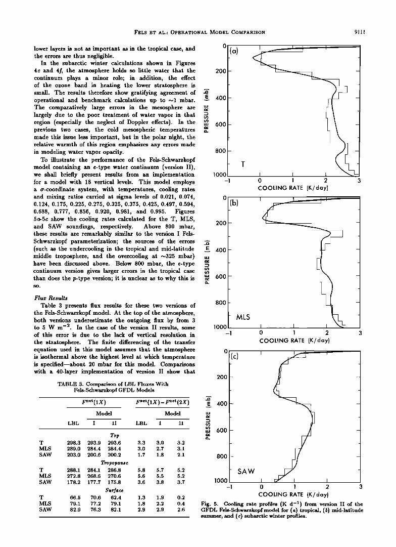
To illustrate the performance of the Fels-Schwarzkopf model contaJninõ an e-type water continuum (version II), we shall briefly present results from an implementation for a model with 18 vertical levels. This model employs a •ocoordinate system, with temperatures, coolinõ rates and mixinõ ratios carried at siõma levels of 0.021, 0.074, 0.124, 0.175, 0.225, 0.275, 0.325, 0.375, 0.425, 0.497, 0.594, 0.688, 0.777, 0.856, 0.920, 0.981, and 0.995. Fiõures 5a-5c show the coolinõ rates calculated for the T, MLS, and SAW soundinõs, respectively. Above 800 mbar, these results are remarkably similar to the version I Felso Schwarzkopf parameterization; the sources of the errors (such as the undercoolinõ in the tropical and mid-latitude middle troposphere, and the overcoolinõ at ~325 mbar) have been discussed above. Below 800 mbar, the e-type continuum version õives larõer errors in the tropical case than does the p-type version; it is unclear as to why this is SO.

Flux Results

Table 3 presents flux results for these two versions of the Fels-Schwarzkopf model. At the top of the atmosphere, both versions underestimate the outõGinõ flux by from 3 to 5 W m -2. In the case of the version II results, some of this error is due to the lack of vertical resolution in

the stratosphere. The finite differencinõ of the transfer equation used in this model assumes that the atmosphere is isothermal above the hiõhest level at which temperature is specified--about 20 mbar for this model. Comparisons with a 40-layer implementation of version II show that

TABLE 3. Comparison of LBL Fluxes With Fels-Schwarzkopf GFDL Models

Model Model

LBL I II LBL I

Top T 298.3 293.9 293.6 3.3 3.0 MLS 289.0 284.4 284.4 3.0 2.7 SAW 203.0 200.6 200.2 1.7 1.8

Tropopause T 288.1 284.1 286.8 5.8 5.7 MLS 272.8 268.6 270.6 5.6 5.5

SAW 178.2 177.7 175.8 3.6 3.8

Surface T 66.5 70.6 62.4 1.3 1.9

MLS 79.1 77.2 79.1 1.8 2.2 SAW 82.9 76.3 82.1 2.9 2.9

3.2

3.1

2.1

5.2

5.2

3.7

0.2

0.4

2.6

200

400

600

8OO

T

1000 _ -1 0 1 2 3

COOLING RATE (K/clay)

200

400

600

800

lOOO

200

l:: 400

600

(c)

MLS

800

1000 -1

SAW

I I

o 1 2

COOLING RATE {K/day}

I I

0 1 2

COOLING RATE (K/dayl

Fig. 5. Cooling rate profiles (K d -1) from version II of the GFDL Fels-Schwarzkopf model for (a) tropical, (b) mid-latitude summer, and (c) subarctic winter profiles.


about 2 W m -2 of the error can be accounted for by this mechanism. At the tropopause, the calculations using version I similarly make errors in the net flux of 3-5 W m -2 while the version II implementation results in a smaller error. At the surface, the version II calculations also appear to result in smaller errors, except for the tropical calculations.

Differences in the forcing due to doubled CO2 at the top of the atmosphere, tropopause, and surface are remarkably similar to those obtained for the Manabe-Stone simulations, with the present version I calculations being similar to the Manabe-Stone version I results, and the present version II calculations paralleling the version III Manabe-Stone results. Thus, the large difference between the Fels- Schwarzkopf version I and II surface flux sensitivities reflects the omission of the 10-#m band of CO2 in the parameterized calculations; calculations using the e-type continuum actually give more realistic sensitivities than those of version I.

5. NCAR COMMUNITY CLIMATE MODEL

VERSION 0 (CCM0) RESULTS Over the past 7 years, two versions (0 and 1) of the

NCAR CCM have been made available to the atmospheric science community. The CCM is a spectral model that has been run at a number of horizontal resolutions. The

model employs a •-vertical coordinate system. CCM0 was made available to the community in 1983 and has been used for a large number of climate and forecast studies. It has been employed in CO2 climate studies [Washington and Meehl, 1983, 1984]. A study of the impact of radiative processes on the climate simulation produced by the model was carried out by Ramanathan et al. [1983]. Numerous paleoclimate studies also have been performed with the model [Barron and Washington, 1982, 1984; Kutzbach and Guetter, 1986]. The response of the model to imposed sea- surface temperature anomalies was studied by Blackmon et al. [1983, 1986.]. Forecast studies include the work of Errico [1984], Baumhe/ner [1983], and Rasch [1985a, b].

CCMO Model Description The nine sigma levels in CCM0 are located at 0.991,

0.926, 0.811, 0.664, 0.500, 0.336, 0.189, 0.074, and 0.009. The longwave radiation scheme employed in CCM0 is described by Ramanathan et al. [1983]. The method for calculating longwave fluxes and heating rates is based on the absorptivity-emissivity formulation. The absorption due to water vapor, carbon dioxide, and ozone is represented by analytical functions of the absorption for the entire band structure. The frequency range is assumed to extend from 0 to 2200 cm-1.

The longwave fluxes due to water vapor are based on the scheme of Sasamori [1968]. However, the treatment of the emissivity for this scheme was modified by Ramanathan et al. [1983] to differentiate between the absorptivity and emissivity. Essentially, the emissivity was determined by dividing the absorptivity by a factor dependent on the pressure-scaled water vapor amount. The functional form of this factor was obtained by fitting data from the Rodgers and Walshaw [1966] band model. Sasamori's scheme does not exphcitly account for the absorption by the e-type continuum. However, it is not clear from the description of the model whether continuum absorption has been accounted for or not. It has been recognized for some time that this continuum plays a significant radiative role in

the lower troposphere. As we shall see, this leads to large differences between the lower tropospheric cooling rates in CCM0 as compared to CCM1.

The radiative treatment of carbon dioxide is based on

the broadband model of Rarnanathan [1976]. The CCM0 broadband model explicitly assumes that all bands in the 15-#m band system overlap one another and that these bands are in the square root limit. The method also explicitly accounts for the temperature dependence of the "hot" bands. Overlap between CO2 and H20 rotational lines is accounted for by multiplying the CO2 band absorptance by the H20 transmissivity obtained from the Rodgers and Walshaw model. No overlap between the e-type continuum and the CO2 absorption is included. Ozone is included by employing the band absorptance model of Rodgers [1968].

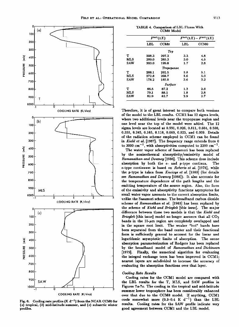
Cooling Rate Results The coohug rates from CCM0 are compared with LBL

cooling rates for the T, MLS, and SAW profiles in Figures 6a-6c. Once again, these results are dependent on the level structure employed, but it is apparent that the model severely underpredicts the cooling in the lower tropical troposphere by as much as 1 K d -1 which may be related to the manner in which the continuum is included

or excluded in the Sasamori water vapor scheme. For the SAW profile, CCM0 actually cools slightly more in the lower troposphere than the LB L results.

Flux Results

Flux results for CCM0 appear in Table 4. The results for the net flux at the tropopause suggest significant differences between the LBL results and the CCM0 model. However, as will be shown later, the fluxes at this level are very sensitive to the model level structure. This conclusion is

also supported by the good agreement between the CCM0 model and the LBL results for the top of the atmosphere (within 1.5 W m-a).

The results for the surface-troposphere forcing due to doubled CO2 indicate that CCM0 is in good agreement with the LBL results (with errors of less than 14%). This agreement, however, must be viewed with some caution, since the actual location of the tropopause in the nine-level model CCM0 is difficult to determine. Kiehl and Briegleb [this issue] compare results from CCM0 employing the ICRCCM MLS profile and find larger differences between CCM0 and the LBL results than appear in Table 4. At the surface, the neglect of the water vapor overlap with the 15-#m CO2 band [Kiehl and Rarnanathan, 1982] results in a substantial overestimation of the flux change for the tropical and mid-latitude profiles. For the subarctic winter profile, agreement between CCM0 and the LBL results is quite good, since water vapor overlap is not important for this particular sounding.

6. NCAR COMMUNITY CLIMATE MODEL

VERSION 1 (CCM1) RESULTS CCM1 Model Description

CCM1 was released for community use in 1987. The model has been used in a stratospheric version for a number of studies [Boville, 1986; Boville and Randel, 1986; Kiehl and Boville, 1988; Kiehl et al., 1988]. One of the most significant differences between CCM0 and CCM1 is actually related to changes in the longwave radiation scheme employed in these two versions of the CCM.

FEL$ ET AL.: OPERATIONAL MODEL COMPARISON 9113

100

200

300

400

5OO

600 -

700 -

800 -

900 -

lOOO -1

(o)

• I • IJ 1 2


1DO

200

300

4OO

5OO

600

700 -

800 -

900 -

lOOO -1

MLS

J I J I 0 1


f I • • i l (c)

100 - -

200 - -

300 - -

-• 400 - -

•' 500 - -

'" 600 - -

700 - -

800 - -

_

9oo - SAW 1000 • I I •

-1 0 1 2 3


Fig. 6. Cooling rate profiles (K d -1) from the NCAR CCM0 for (a) tropical, (b) mid-latitude summer, and (c) subarctic winter profiles.

TABLE 4. Comparison of LBL Fluxes With CCM0 Model

F"e' (1X) rne'(1X)-Fne'(2X) LBL CCM0 LBL CCM0

Top T 298.3 297.3 3.3 4.8 MLS 289.0 285.3 3.0 4.5

SAW 203.0 199.8 1.7 2.8

Tropopause T 288.1 292.5 5.8 5.1 MLS 272.8 268.7 5.6 5.0

SAW 178.2 185.9 3.6 3.2

T 66.5 87.2 1.3 2.6

MLS 79.1 88.1 1.8 2.8 SAW 82.9 82.7 2.9 2.7

Therefore, it is of great interest to compare both versions of the model to the LBL results. CCM1 has 12 sigma levels, where two additional levels near the tropopause region and one level near the top of the model were added. The 12 sigma levels are located at 0.991, 0.926, 0.811, 0.664, 0.500, 0.355, 0.245, 0.165, 0.110, 0.060, 0.025, and 0.009. Details of the radiation scheme employed in CCM1 can be found in Kiehl et al. [1987]. The frequency range extends from 0 to 3000 cm -1 with absorptivities computed to 2200 cm -1 ,

The water vapor scheme of Sasamori has been replaced by the nonisothermal absorptivity/emissivity model of Ramanathan and Downey [1986]. This scheme does include absorption by both the e- and p-type continua. The e-type continuum is based on Roberts et al. [1976], while the p-type is taken from Kneizys et al. [1980] (for details see Ramanathan and Downey [1986]). It also accounts for the temperature dependence of the path lengths and the emitting temperature of the source region. Also, the form of the emissivity and absorptivity functions asymptotes for small water vapor amounts to the correct absorption limits, unlike the Sasamori scheme. The broadband carbon dioxide

scheme of Ramanathan et al. [1983] has been replaced by the scheme of Kiehl and Briegleb [this issue]. The major difference between these two models is that the Kiehl and

Briegleb [this issue] model no longer assumes that all CO2 bands in the 15-/•m region are completely overlapped and in the square root limit. The weaker "hot" bands have been separated from the band center and their functional form is sufficiently general to account for the linear and logarithmic asymptotic limits of absorption. The ozone absorption parameterization of Rodgers has been replaced by the broadband model of Ramanathan and Dickinson [1979]. Finally, the numerical algorithm for evaluating the integral exchange term has been improved in CCM1; nearest layers are subdivided to increase the accuracy of evaluating the absorption functions over that layer.

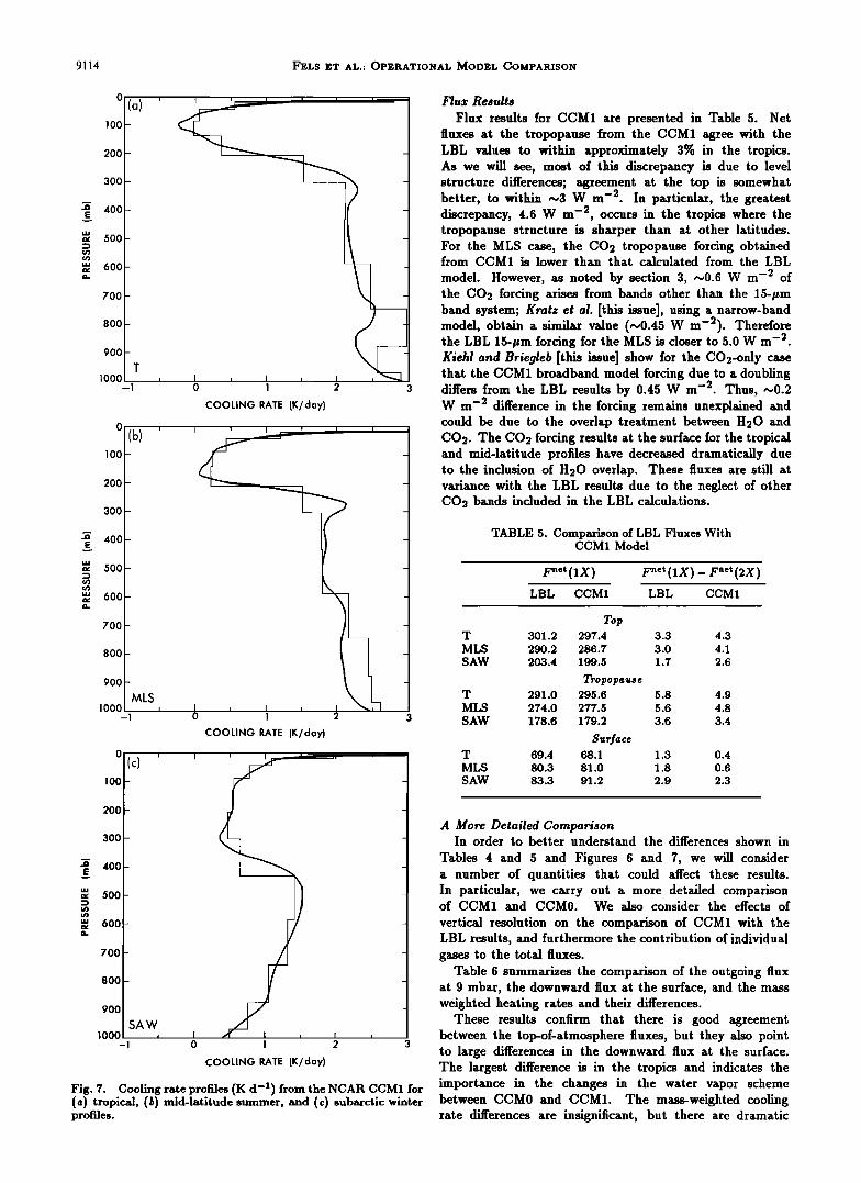
Cooling Rate Results Cooling rates for the CCM1 model are compared with

the LBL results for the T, MLS, and SAW profiles in Figures 7a-7c. The cooling in the tropical and mid-latitude summer lower troposphere has been considerably enhanced over that due to the CCM0 model. If anything, CCM1 cools somewhat more (0.3-0.4 K d -1) than the LBL results. Cooling rates for the SAW profile indicate very good agreement between CCM1 and the LBL model.


]øø 200 300

400 soo

600

7OO

8OO

9OO

IOO0 -1 0 1 2 3


200 -

300 -

400 -

500 -

600 -

700 -

800

900

lOOO MLS, I , • , • -I -1 0 1 2 3


0

100 -

200 -

300 -

400 -

500 -

600 -

700 -

800 -

900 -

SAW 1000 ,

' I

_

_

_

_

I • I , 0 1 2 3


Fig. 7. Cooling rate profiles (K d -•) from the NCAR CCM1 for (a) tropical, (b) mid-latitude summer, and (c) subarctic winter profiles.

Flux Results

Flux results for CCM1 are presented in Table 5. Net fluxes at the tropopause from the CCM1 agree with the LBL values to within approximately 3% in the tropics. As we will see, most of this discrepancy is due to level structure differences; agreement at the top is somewhat better, to within ~3 W m -2. In particular, the greatest discrepancy, 4.6 W m -2 occurs in the tropics where the tropopause structure is sharper than at other latitudes. For the MLS case, the CO2 tropopause forcing obtained from CCM1 is lower than that calculated from the LBL

model. However, as noted by section 3, ~0.6 W m -2 of the CO2 forcing arises from bands other than the 15-/•m band system; Kratz et al. [this issue], using a narrow-band model, obtain a similar value (~0.45 W m-2). Therefore the LBL 15-/•m forcing for the MLS is closer to 5.0 W m -2. Kiehl and Briegleb [this issue] show for the CO2-only case that the CCM1 broadband model forcing due to a doubling differs from the LBL results by 0.45 W m -2. Thus, ~0.2 W m -2 difference in the forcing remains unexplained and could be due to the overlap treatment between H20 and CO2. The CO2 forcing results at the surface for the tropical and mid-latitude profiles have decreased dramatically due to the inclusion of H20 overlap. These fluxes are still at variance with the LBL results due to the neglect of other CO2 bands included in the LBL calculations.

TABLE 5. Comparison of LBL Fluxes With CCM1 Model

LBL CCM1 LBL CCM1

Top T 301.2 297.4 3.3 4.3

MLS 290.2 286.7 3.0 4.1 SAW 203.4 199.5 1.7 2.6

Tropopause T 291.0 295.6 5.8 4.9 MLS 274.0 277.5 5.6 4.8 SAW 178.6 179.2 3.6 3.4

S•r/•ce T 69.4 68.1 1.3 0.4

MLS 80.3 81.0 1.8 0.6 SAW 83.3 91.2 2.9 2.3

A More Detailed Comparison In order to better understand the differences shown in

Tables 4 and 5 and Figures 6 and 7, we will consider a number of quantities that could affect these results. In particular, we carry out a more detailed comparison of CCM1 and CCM0. We also consider the effects of

vertical resolution on the comparison of CCM1 with the LBL results, and furthermore the contribution of individual gases to the total fluxes.

Table 6 summarizes the comparison of the outgoing flux at 9 mbar, the downward flux at the surface, and the mass weighted heating rates and their differences.

These results confirm that there is good agreement between the top-of-atmosphere fluxes, but they also point to large differences in the downward flux at the surface. The largest difference is in the tropics and indicates the importance in the changes in the water vapor scheme between CCM0 and CCM1. The mass-weighted cooling rate differences are insignificant, but there are dramatic


TABLE 6. Comparison of CCM0 and CCM1 Fluxes Using Same Level Structure From McClatchey Profiles

CCM1 CCM0 A

T

F(top) 303.2 303.8 0.6 F(surf) 391.2 372.0 -19.2 q -1.9 -1.8 0.1

MLS

F(top) 292.9 293.0 0.1 F(surf) 342.6 335.5 -7.1 q -1.7 -1.6 0.1

SAW

F(top) 203.6 205.4 1.8 F(surf) 156.6 165.0 8.5 q --0.9 -1.0 -0.1

differences in the vertical heating between the two models. This is illustrated in Figures 8a-8c, where the heating rates for the three atmospheric profiles are shown for CCM0 and CCM1. For the tropical profile, heating differences in the lower troposphere are as large as i K d -1. For the MLS profile, differences are still large (greater than 0.5 K d -1) where CCM1 cools more than CCM0. For the SAW profile, CCM1 actually cools less than the CCM0 model. These results indicate the value of considering the surface radiative fluxes for model validation purposes, since the top-of-atmosphere fluxes are less sensitive to the H20 continuum absorption.

The question remains as to how important differences in the vertical resolution are to the comparison of operational model results and the LBL results. To address this issue, fluxes from the CCM1 model have been evaluated on the same high-resolution vertical grid that was employed for the LBL calculations. Table 7 compares the net fluxes at three levels of the two models for the tropical profile; also included are the mass-weighted atmospheric heating rates from the models.

The agreement between these two models is now much better at the tropopause than was found in Table 5. This indicates that differences in vertical resolution are the main

source of differences between CCM1 and LBL absolute

fluxes. To further understand the differences in Table 7, the total fluxes have been broken down into contributions

from individual gases. Table 8 lists the values of the net flux at the tropopause for the tropical profile for water vapor and carbon dioxide. Further comparisons for CO2 are presented by Kiehl and Briegleb [this issue]. Differences due to ozone are much smaller than those due to either of

these gases. The results of Table 8 indicate that the major source

of the differences arises from the water vapor treatment. This is most likely due to the narrow-band model data employed by Ramanathan and Downey [1986] to obtain their parameterization, which used a random model with a 5 cm -1 interval width. It is now recognized [Schwarzkopf and Fels, this issue] that a random model interval width of 10 cm -1 is more appropriate for water vapor transmission calculations for these types of models. Finally, another source of bias could arise from the overlap treatment of the gases, which is an inherent problem with broadband models.

Summary These results indicate that a significant improvement

in modehng longwave radiative processes in the CCM

0

100 -

200 -

300 -

400-

500 -

600 -

700 -

800 -

900 -

lOOO I , I

•- -- i I I

,, i

i i i

ß II


0 ,

100 -

200 -

300 -

400 -

500 -

600 -

700 -

800 -

900 -

MLS 1000

I ,i I ' I I

f--J i

!

1 2 3


0 ,

100 -

200 -

300 -

400 -

500 -

600 -

700 -

800 -

900 -

SAW 1000 ,

I I i ' II I I

I' L•


Fig. S. Cooling rate profiles (K d -1) from CCMO (dashed line) and CCM1 (•ond nn•) for (•) tropical, (b) mid-latitude summer, and (c) subarctic winter profiles.


TABLE 7. Compaxison of LBL and CCM1 Absolute Fluxes Employing Same High Vertical

Resolution Grid on a Tropical Sounding

LBL CCM1 A

vnet(top) 301.2 302.2 1.0 vnet (trop) 291.0 293.2 2.2 vnet (surf) 69.4 71.9 2.5 q -1.9 -1.9 0.0

TABLE 8. Flux Contributions From CO2 and H20 for LBL and CCM1

LBL CCM1 A

H•. O 334.4 336.3 1.9 CO2 405.1 404.3 -0.8

The sensitivity of the GISS GCM to climate forcing and feedback analysis is presented by Hansen et al. [1984] for doubled CO2, for a 2% solar constant increase, and for Ice Age simulations. Model simulations of transient climate change due to the anthropogenic increase of CO2 and other trace gases, along with projections into the future, are compared with the observed global temperature record by Hansen et al. [1988]. Other studies describing climate simulations with the GISS GCM include analysis of doubled CO2 experiment results by Rind [1987a, 1988] and of paleoclimate simulations by Rind and Peteet [1985] and Rind [1986, 1987b]. Application of the GISS GCM radiation model for stratospheric modeling is described by Rind et al. [1988].

The radiative algorithm described above has been ap- plied to two different vertical layer structures, set according to the sigma-level prescription used in the tropospheric and stratospheric versions of the GISS GCM. The results com-

has occurred in going from version 0 to version 1. The puted with the tropospheric 12-layer version are designated majority of this improvement was achieved by employing as "model A" results, while those for the stratospheric the Ramanathan and Downey water vapor scheme. Changes 25-layer version are designated as "model B" results. It in the level structure and in the vertical finite difference should be emphasized that cooling rates from models A scheme have also aided in the accuracy of the cooling rate and B are calculated using the same radiative model and calculations. the same set of k-distribution absorption coefficient tables.

7. GODDARD INSTITUTE FOR SPACE STUDIES Cooling Rate Results MODEL RESULTS Cooling rates computed with model A are shown in

(MODEL II [Hansen et al., 1983]) Figures 9a-9c for the T, MLS, and SAW temperature Model Description and Usage profiles. The GCM results are generally in good agreement

The Goddard Institute for Space Studies (GISS) GCM with the LBL results, particularly for the SAW profile, radiation model has been used for climate modeling in where agreement is very close throughout the atmosphere. basically unaltered form since 1983. It is described briefly In the case of the T and MLS profiles, the upper by Hansen et al. [1988], and has been used primarily tropospheric and stratospheric cooling rates closely follow for tropospheric modeling with nine sigma layers between the LBL results, but there is a marked overestimate of the ground and 10 mbar. cooling below the 800-mbar pressure level. Surprisingly,

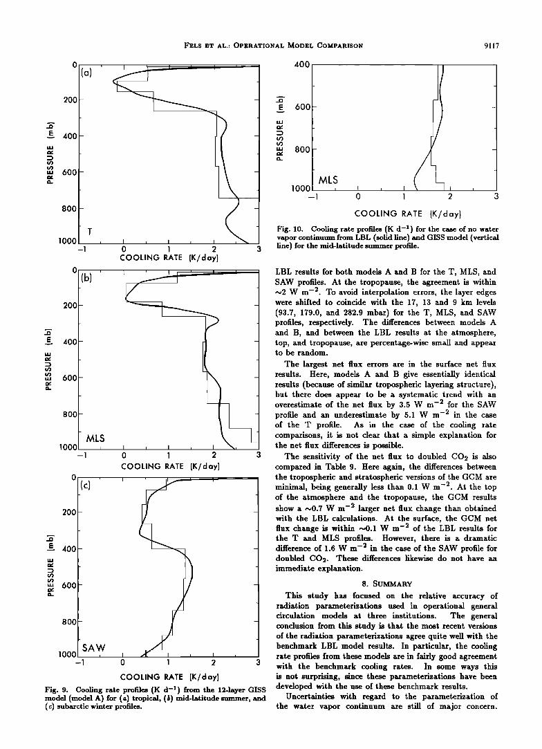
A detailed description of the radiation scheme is given the error appears largely to result from the computation of by Lacis and Oinas [this issue]. Integration over the cooling rates due to absorption lines, not in the formulation thermal spectrum utilizes the correlated k-distribution of the water vapor continuum. Figure 10 shows that the method to treat gaseous absorption and emission in a ~0.5 K d -1 cooling rate error persists in the lower two vertically inhomogeneous atmosphere. The model uses 11 model layers even for the noncontinuum case for the MLS composite k-distribution intervals for H20, 10 for CO2, profile. The reasons for this error (and the good agreement and four for Os to cover the thermal spectrum. Absorption for the SAW profile) are unclear. coefficients in these composite intervals are determined Figures 11a-11c show a comparison of cooling rates by merging Planck function weighted narrow band k- using model B for the T, MLS, and SAW profiles. All distributions (~50 cm -1) from noncontiguous spectral three profiles show good agreement with the LBL results regions. The narrow band k-distributions are obtained below ~1 mbar, although the GCM results for the T from Malkmus model parameters that are least squares and MLS profiles still overestimate the near-surface cooling fitted to LBL transmissions calculated using the AFGL as in the case of the tropospheric model. The T line compilation [Rothman, 1981] for a grid of pressure and MLS cooling is in general agreement with the LBL and temperature combinations. Absorption contributions results up to the 0.1-mbar level, while the SAW profile due to cH4, N20, CFCls, and CF2C12 and the weaker results overestimate the cooling by 2-3 K d -1. Part bands of H20, CO2, and Os are included as absorption of the cooling rate difference with respect to the LBL overlapping. Water vapor continuum absorption is included cooling above the 1-mbar level stems from differences using the formulation and spectral dependence given by in the pressure-temperature interpolation method of the Roberts et al. [1976]. Absorption coefficients representing McClatchey temperature profiles between the GCM and the merged k-distribution intervals are interpolated as LBL calculations. Undoubtedly, as in the case of the functions of pressure, temperature, and absorber amount GFDL model, errors in modeling the water vapor opacity from a large table of Planck function weighted coefficients. also contribute to these differences. The atmospheric temperature profile is specified at layer edge points and is assumed to be linear in Planck function Flux Results within the layer interior. This permits the integrated Table 9 compares the net fluxes computed for models thermal emission from the entire layer to be obtained A and B against LBL results for the three standard in closed form. The frequency range extends from 0 to temperature profiles. The net fluxes at the top of the 2500 cm -1. atmosphere are found to agree within ~1 W m -2 of the

FEL$ ET AL.: OPElrATIONAL MODEL COMPAttI$ON 9117

Ot(a) , • , 400 200 ._.. 600 -

. • 400

800,-

,,'e, 600

• 1000 1ME, S I i

3

800 t COOLING RATE (K/day) Z ris. 10. Cooling rate profiles (K d -•) for the case of no water 1000 J , vapor continuum from LBL (solid line) and GISS model (vertical

-1 0 1 2 3 line) for the mid-latitude summer profile. COOLING RATE (K/day)

0 , I (b)

200 -

400

600

8OO

-ML,S 1000• • --1 0 1 2 3


200

400

6OO

800

i

SA,W

i

o 1 2


lOOO

Fig. 9. Cooling rate profiles (K d -1) from the 12-layer GISS model (model A) for (•) tropical, (b) mid-latitude summer, and (c) sub•rctic winter profiles.

LBL results for both models A and B for the T, MLS, and SAW profiles. At the tropopause, the agreement is within ~2 W m -2. To avoid interpolation errors, the layer edges were shifted to coincide with the 17, 13 and 9 km levels (93.7, 179.0, and 282.9 mbar) for the T, MLS, and SAW profiles, respectively. The differences between models A and B, and between the LBL results at the atmosphere, top, and tropopause, are percentage-wise small and appear to be random.

The largest net flux errors are in the surface net flux results. Here, models A and B give essentially identical results (because of similar tropospheric layering structure), but there does appear to be a systematic trend with an overestimate of the net flux by 3.5 W m -2 for the SAW profile and an underestimate by 5.1 W m -2 in the case of the T profile. As in the case of the coohug rate comparisons, it is not clear that a simple explanation for the net flux differences is possible.

The sensitivity of the net flux to doubled CO2 is also compared in Table 9. Here again, the differences between the tropospheric and stratospheric versions of the GCM are minimal, being generally less than 0.1 W m -2. At the top of the atmosphere and the tropopause, the GCM results show a ~0.7 W m -2 larger net flux change than obtained with the LBL calculations. At the surface, the GCM net flux change is within ~0.1 W m -2 of the LBL results for the T and MLS profiles. However, there is a dramatic difference of 1.6 W m -2 in the case of the SAW profile for doubled CO2. These differences hkewise do not have an immediate explanation.

8. SUMMARY

This study has focused on the relative accuracy of radiation parameterizations used in operational general circulation models at three institutions. The general conclusion from this study is that the most recent versions of the radiation parameterizations agree quite well with the benchmark LBL model results. In particular, the coohug rate profiles from these models are in fairly good agreement with the benchmark cooling rates. In some ways this is not surprising, since these parameterizations have been developed with the use of these benchmark results.

Uncertainties with regard to the parameterization of the water vapor continuum are still of major concern.


.01 a) • i

.10

1.0

lO

lOO

1000 • • I I I I I I --2 0 2 4 6 8 10 12 14

COOLING RATE (K/day}

.01

.10

lO

lOO -

lOOO -2

i I i i

• MLS 0 2 4 6 8 10 12 14

COOLING RATE (K/day} 16

.01 i J jl

• 10

_

_

lOO - _

_

SAW 1000 I I I I I I -

-2 0 2 4 6 8 10 12 14 16


Fig. 11. Cooling rate profiles (K d -1) from the 25-layer GISS model (model B) for (a) tropical, (b) mid-latitude summer, and (c) subarctic winter profiles.

TABLE 9. Comparison of Fluxes From the GISS GCM With Line-by-Line Results

rnet(1X) Fnet (lX)- F •(et (2X) Model Model

LBL A B LBL A B

Top T 299.0 297.6 298.4 3.2 4.0 4.1 MLS 289.5 290.2 290.1 3.0 3.7 3.8

SAW 203.1 202.5 202.7 1.7 2.3 2.2

Tropopause T 288.7 286.9 288.8 5.8 6.7 6.7

MLS 273.3 274.7 274.7 5.6 6.5 6.4 SAW 178.3 180.4 179.8 3.6 4.3 4.3

Surface T 67.1 62.0 62.0 1.3 1.2 1.2 MLS 79.5 77.3 77.4 1.8 1.9 1.9 SAW 83.0 86.5 86.5 2.9 4.5 4.5

The importance of this process to tropical and mid- latitude lower tropospheric cooling is significant and can be important in the simulation of convective activity in the general circulation models. It is important that our knowledge of this process be extended in the next few years. It is also apparent from this study that an attempt should be made to parameterize the weaker absorption bands of CO2 and 03, in order to obtain more accurate agreement with the LBL results.

As with any parameterization process, the development of radiation codes is not static. We hope that as newer versions of operational model radiation codes become available, they are continually compared with benchmark calculations and improved observational data, and that the results of these comparisons be made available to the general circulation modeling community.

Acknowledgments. It is unfortunate that during the prepa- ration of this manuscript, Steve Fels passed away. Steve asked me (J.T.K.) to assume responsibility for the completion of the manuscript a month before his death. Much of the study carries with it the mark of his erudite style; he shall be missed by his friends and colleagues. J.T.K. would like to thank Bruce Briegleb for preparing the NCAR CCM results. The National Center for Atmospheric Research is sponsored by the National Science Foundation.

REFERENCES

Barron, E. J., and W. M. Washington, The Cretaceous atmospheric circulation: Comparisons of model simulations with the geologic record, Paleogeogr. Paleoclim. Paleoecol., ,tO, 103-133, 1982.

Barron, E. J., and W. M. Washington, The role of geographic variables in explaining paleoclimates: Results from Cretaceous climate model sensitivity studies, J. Geophys. Res., 89, 1267- 1279, 1984.

Baumhefner, D. P., Relationship between present large-scale forecast skill and new estimates of predictability error growth, Pro- ceedings, Workshop on Predictability of Fluid Motions, vol. 106, pp. 169-180, Am. Inst. of Phys., New York, 1983.

Bignell, K. J., The water-vapour infra-red continuum, Q. J. R. Meteorol. Soc., 96, 390-403, 1970.

Blackmon, M. L., J. E. Geisler, and E. J. Pitcher, A general circulation model study of January climate anomaly patterns associated with interannual variation of equatorial Pacific sea surface temperatures, J. Atmos. Sci., ,t3, 1410-1425, 1983.

Blackmon, M. L., S. L. Mullen, and G. T. Bates, The climatology of blocking events in a persistent January simulation with a spectral general circulation model, J. Atmos. Sci., ,t3, 1379- 1405, 1986.


Boville, B. A., Wave-mean flow interactions in a general circulation model of the troposphere and stratosphere, J. Atmos. Sci., 43, 1711-1725, 1986.

Boville, B. A., and W. J. Randal, Observations and simulation of the variability of the stratosphere and troposphere in January, J. Atmos. Sci., 43, 3015-3034, 1986.

Broccoli, A. J., and S. Manabe, The influence of continental ice, atmospheric CO2, and land albedo on the climate of the last glacial maximum, Clim. D•tn., 1, 87-99, 1987.

Bryan, K., F. G. Komro, S. Manabe, aad M. J. Speltnan, Tran- sient climate response to increasing atmospheric carbon dioxide, Science, •15, 56-58, 1982.

Bryan, K., S. Manabe, and M. J. Spelman, Interhemispheric asymmetry in the transient response of a coupled ocean- atmosphere model to a CO2 forcing, J. Phsts. Oceanogr., 18, 851-867, 1988.

Drayson, S. R., Atmospheric transmission in the CO2 bands between 12/z and 18/z, App/. Opt., 5, 385-391, 1973.

Ellingson, R. G., J. Ellis, and S. Fels, The intercomparison of r•- diation codes in climate models: Longwave results, J. Geophlts. Res., this issue.

Errico, R., The dynamical balance of a general circulation model, Mon. Weather Rev., 11•, 2439-2454, 1984.

Fels, S. B., Simple strategies for inclusion of Voigt effects in infrared cooling calculations, AppL Opt., 18, 2634-2637, 1979.

Fels, S. B., Analytic representations of standard atmosphere temperature profiles, J. Atmos. Sci., J3, 219-221, 1986.

Fels, S. B., and M.D. Schwarzkopf, The simplified exchange approximation: A new method for radiative transfer calculations, J. Atmos. Sci., 3•, 1475-1488, 1975.

Fels, S. B., and M.D. Schwarzkopf, An efficient, accurate algorithm for calculating CO2 15-/•m band cooling rates, J. Geo- i0h!ts. Res., 86, 1205-1232, 1981.

Fels, S. B., J. D. Mahlman, M.D. Schwarzkopf, and R. W. Sin- clair, Stratospheric sensitivity to perturbations in ozone and carbon dioxide: Radiative and dynamical response, J. Atmos. Sci., 37, 2265-2297, 1980.

Goody, R. M., Atmospheric Radiation, 436 pp., Oxford Univer- sity Press, New York, 1964.

Hamilton, K., and J. D. Mahlman, General circulation model simulation of the semiamaual oscillation of the tropical middle atmosphere, J. Atmos. Sci., J5, 3212-3235, 1988.

Hansen, J. G., G. Russell, D. Rind, P. Stone, A. Lacis, S. Lebed- eft, R. Ruedy, and L. Travis, Efficient three-dimensional global models for climate studies: Models I and II, Mon. Weather Rev., 111, 609-662, 1983.

Hansen, J., A. Lacis, D. Rind, G. Russell, P. Stone, I. Fung, R. Ruedy, and J. Lerner, Climate sensitivity: Analysis of feedback mechanisms, in Climate Processes and Climate Sensitiv- ity, Geophlts. Monogr., •9,, edited by J. E. Hansen and T. Ta&.ahashi, pp. 130-163, AGU, Wa.shington, D.C., 1984.

Hansen, J., I. Fung, A. Lacis, D. Rind, S. Lebedeff, R. Ruedy, and G. Russell, Global climate changes as forecast by Goddard In- stitute for Space Studies three-dimensional model, J. Geoph!ts. Res., 93, 9341-9364, 1988.

Hayashi, Y., D. Golder, and J. D. Mahlrnan, Stratospheric and mesospheric Kelvin waves simulated by the GFDL "SKYHI" general circulation model, J. Atmos. Sci., 41, 1971-1984, 1984.

Kiehl, J. T., and B. A. Boville, The radiative-dynamical response of a stratospheric-tropospheric general circulation model to changes in ozone, J. Atmos. Sci., J5, 1798-1817, 1988.

Kiehl, J. T., and B. P. Briegleb, A new parameterization of the absorptance due to the 15-/•m band system of carbon dioxide, J. Geophl•s. Res., this issue.

Kiehl, J. T., and V. Ramanathan, Radiative heating due to increased CO2: The role of H20 continuum absorption in the 12-18/•m region, J. Atmos. Sci., 39, 2923-2926, 1982.

Kiehl, J. T., B. A. Boville, and B. P. Briegleb, Response of a general circulation model to a prescribed Antarctic ozone hole, Nature, 33•, 501-504, 1988.

Kiehl, J. T., R. J. Wolski, B. P. Briegleb, and V. Ramanathan, Documentation of radiation and cloud routines in the NCAR

Community Climate Model (CCM1), National Center for At- mospheric Research, NCAR Tech. Note NCAR/TN-•88+IA, 109 pp., Boulder, Colo., 1987. (Available as NTIS PB88- •3611•/AS from Natl. Tech. Inf. Serv., Springfield, Va.)

Kneizys, F. X. et al., Atmospheric transmittance radiance

•computer code LOWTRAN5, Environ. Res. Pap. No. 697, AFGL-TR-80-0067, 233 pp., Air Force Geophys. Lab., Bed- ford, Mass., 1980.

Kratz, D. P., B.-C. Gao, and J. T. Kiehl, A study of the radiative effects of the 9.4 and 10.4 micron bands of carbon dioxide, J. Geophsts. Res., this issue.

Kutzbach, J. E., and P. J. Guetter, The influence of changing orbital parameters and surface boundary conditions on climate simulations for the past 18,000 years, J. Atmos. Sci., 43, 1726- 1759, 1986.

Lacis, A. A., and V. Oinas, A description of the correlated k- distribution method for modeling nongray gaseous absorption, thermal emission, and multiple scattering in vertically inhomogeneous atmospheres, J. Geophsts. Res., this issue.

Mahlman, J. D., and L. J. Umscheid, Dynamics of the middle atmosphere: Successes and problems of the GFDL "SKYHI" general circulation model, in Dltnamics o] the Middle Atmo- sphere, edited by J. R. Holton and T. Matsuno, pp. 501-526, Terra Scientific Publishing, Terrapub, Tokyo, 1984.

Mahlman, J. D., and L. J. Umscheid, Comprehensive modeling of the middle atmosphere: The influence of resolution, in Trans- port Processes in the Middle Atmosphere, edited by G. Vis- conti and R. Garcia, pp. 251-266, D. Reidel, Hingham, Mass., 1987.

Manabe, S., and A. J. Broccoli, A comparison of climate model sensitivity with data from the last glacial maximum, J. Atmos. Sci., 4•, 2643-2651, 1985.

Manabe, S., and R. J. Stouffer, A CO2-climate sensitivity study with a mathematical model of the global climate, Nature, •8•, 491-493, 1979.

Manabe, S., and R. J. Stouffer, Sensitivity of a global climate model to an increase in CO2 content of the atmosphere, J. Geophlts. Res., 85, 5529-5554, 1980.

Manabe, S., and R. T. Wetheraid, The effects of doubling of CO2 concentration on the climate of a general circulation model, J. Atmos. Sci., 3•, 3-15, 1975.

Manabe, S., and R. T. Wetherald, Large-scale changes in soil wetness induced by an increase in atmospheric carbon dioxide, J. Atmos. Sci., 44, 1212-1235, 1987.

McClatchey, R. A., R. W. Faun, J. E. A. Selby, F. E. Volz, and J. S. Gazing, Optical properties of the atmosphere, Environ. Res. Pap. No. 411, AFCRL-72-0497,108 pp., Air Force Cambridge Res. Lab., Bedford, Mass., 1972.

Miyahara, Y., Y. Hayashi, and J. D. Mahlman, Interactions between gravity waves and planetary-scale flow simulated by the GFDL "SKYHI" general circulationmodel, J. Atmos. Sci., 43, 1844-1861, 1986.

Ramanathan, V., Radiative transfer within the earth's troposphere and stratosphere: A simplified radiative-convective model, J. Atmos. Sci., 33, 1330-1346, 1976.

Ramanathan, V., and R. E. Dickinson, The role of stratospheric ozone in the zonal and seasonal radiative energy balance of the earth-troposphere system, J. Atmos. Sci., 36, 1084-1104, 1979.

Ramanathan, V., and P. Downey, A nonisothermal emissivity and absorptivity formulation for water vapor, J. Geophsts. Res., 91, 8649-8666, 1986.

Ramanathan, V., E. J. Pitcher, R. C. Malone, and M. L. Black- mon, The response of a spectral general circulation model to improvements in radiative processes, J. Atmos. Sci., 40, 605- 630, 1983.

Rasch, P. J., Developments in normal mode initialization, Part I, A simple interpretation for normal mode initialization, Mon. Weather Rev., 113, 1746-1753, 1985a.

Rasch, P. J., Developments in normal mode initialization, Part II, A new method and its comparison with currently used schemes, Mon. Weather Rev., 113, 1753-1770, 1985b.

Rind, D., The dynamics of waxIn and cold climates, J. Atmos. Sci., 43, 3-24, 1986.

Rind, D., The doubled CO2 climate: Impact of the sea surface temperature gradient. J. Atmos. Sci., 44, 3235-3268, 1987a.

Rind, D., Components of Ice Age circulation, J. Geophps. Res., 9g, 4241-4281, 1987b.

Rind, D., Dependence of waxIn and cold climate depiction on climate model resolution, J. Clim., 1, 965-997, 1988.

Rind, D., and D. Peteat, LGM terrestrial evidence and CLIMAP SSTs: Are they consistent, Quat. Res., •4, 1-22, 1985.


Rind, D., R. Suozzo, N. K. Balachandran, A. Lacis, and G. Rus- sell, The GISS global climate--middle atmosphere model, Part I, Model, structure and climatology, J. Atmos. Sci., •5, 329- 370, 1988.

Roberts, R. E., J. E. Selby, and L. M. Biberman, Infrared continuum absorption by atmospheric water vapor in the 8-12 tzm window, Appl. Opt., 15, 2085-2090, 1976.

Rodgers, C. D., Some extensions and applications of the new random model for molecular band transmission, Q. J. R. MeteoroL Soc., 9•, 99-102, 1968.

Rodgers, C. D., and C. D. Walshaw, The computation of infrared cooling rate in planetary atmosphere, Q. J. R. Meteorol. Soc., 9•, 67-92, 1966.

Rothrnan, L. S., AFGL atmospheric absorption line parameters compilation: 1980 version, Appl. Opt., •0, 791-795, 1981.

Rothrnan, L. S., R. R. Gainache, A. Barbe, A. Goldman, J. R. Gillis, L. R. Brown, R. A. Toth, J. M. Flaud, and C. Camy- Peyret, AFGL atmospheric absorption line parameters compilation: 1982 edition, AppL Opt., •, 2247-2256, 1983.

Saiedy, F., Absolute measurements on infra-red radiation in the atmosphere, Ph.D. thesis, 43 pp., London Univ., 1960.

Sasamori, T., The radiative cooling calculation for application to general circulation experiments, J. AppL MeteoroL, 17, 721- 729, 1968.

Schwarzkopf, M.D., and S. B. Fels, The simplified exchange method revisited: An accurate, rapid method for computation of infrared cooling rates and fluxes, J. Geoph•/s. Res., this issue.

Stone, H. M., and S. Manabe, Comparison among various numerical models designed for computing infrared cooling, Mon. Weather Rev., 96, 735-741, 1968.

Vigroux, F., ]•mission continue de l'atmosph•re terrestre a 9.6tz, Ann. Geoph•ls., 15, 453-460, 1959.

Washington, W. M., and G. A. Meehl, General circulation model experiments on the climatic effects due to a doubling and qua- drupling of carbon dioxide concentration, J. Geoph•/s. Res., 88, 6600-6610, 1983.

Washington, W. M., and (3. A. Meehl, Seasonal cycle experiment on the climate sensitivity due to a doubling of CO2 with an atmospheric general circulation model coupled to a simple mixed-layer ocean model, J. Geoph•/s. Res., 89, 9475-9503, 1984.

Wetherald, R. T., and S. Manabe, Influence of seasonal variation upon the sensitivity of a model climate, J. Geoph•ts. Res., 86, 1194-1204, 1981.

S. B. Fels and M.D. Schwarzkopf, Geophysical Fluid Dynaa•ics Laboratory, NOAA, P. O. Box 308, Princeton University, Prince- ton, NJ 08542.

J. T. Kiehl, Climate Modeling Section, National Center for Atmospheric Research, P. O. Box 3000, Boulder, CO 80307.

A. A. Lacis, NASA Goddard Institute for Space Studies, 2880 Broadway, New York, NY 10025.

(Received July 3, 1990; revised February 22, 1991;

accepted February 22, 1991.)

infrared cooling rate calculations in operational

Documents