information to users - mcgill universitydigitool.library.mcgill.ca/thesisfile36855.pdf · les voies...
TRANSCRIPT

INFORMATION TO USERS
This manuscript has been reproduced from the microfilm master. UMI films
the text directly trom the original or copy submitted. Thus. some thesis and
dissertation copies are in typewriter face, while others may be trom any type of
computer printer.
The quality of thia reproduction la depend.nt upon the quallty of the
copy aubmitted. Broken or indistinct print, colored or poor quality illustrations
and photographs, print bleedthrough, substandard margins, and improper
alignment can adversely affect reproduction.
ln the unlikely event that the author did not send UMI a complete manuscript
and there are missing pages, these will be noted. Also, if unauthorized
copyright material had ta be removed, a note will indicate the deletion.
Oversize materials (e.g., maps, drawings, charts) are reproduced by
sectioning the original, beginning at the upper left...hand corner and continuing
trom left to right in equal sections with small overlaps.
ProQuest Information and Leaming300 North Zeeb Raad, Ann Arbor, MI 48106-1346 USA
8QO...S21-0600


•
•
TRIE rvIETHüDS FOR STRUCTURED DATA ON
SECONDA.RY STORAGE
by
XIAOY:4N ZHAO
School of Computer Science
~IcGill University
~[ontréal. Québec
Canada
October 2000
A DISSERTATION
SUBMITTED TO THE FACULTY OF GRADUATE STUDIES AND RESEARCH
OF wlCGILL UNIVERSITY
IN PARTIAL FULFILLMENT OF THE REQUIREMENTS FOR
THE DEGREE OF DOCTOR OF PHILOSOPHY
Copyright © 2000 by XIAOYAN ZHAO

1"'1 National Libraryof Canada
Acquisitions andBibliographie seNÎCeS
385 welinglon Str••Ottawa ON K1A QN.tc.nadII
BibüoIhèque nationaledu Canada
Acquisitions etseMees bibliographiques
395. rue Wellingtonoa... ON K1A 0N4CaNda
The author bas granted a nonexclusive licence alloWÏDg theNational Library ofCanada toreproduce, loan, distribute or sellcopies of this thesis in microfo~paper or elecuonic formats.
The author retains ownership of thecopyright in this thesis. Neither thethesis nor substantial extracts trom itmay he printed or otherwisereproduced without the author'spermJSSlon.
L'auteur a accordé une licence nonexclusive permettant à laBibliothèque nationale du Canada dereproduire, prêter, distribuer ouvendre des copies de cette thèse sousla fonne de microfiche/film, dereproduction sur papier ou sur formatélectronique.
L'auteur conserve la propriété dudroit d'auteur qui protège cette thèse.Ni la thèse Di des extraits substantielsde celle-ci ne doivent être imprimésou autrement reproduits sans sonautorisation.
0-612-69955-2
Canadl

•
•
Abstract
This thesis presents trie organizations for one-dimensional and rnultidimensional struc
tured data on secondary storage. The new trie structures have several distinctive fea
tures: (1) they provide significant storage compression by sharing cornillon paths near
the root: (2) they are partitioned into pages and are suitable for secondary storage:
(3) they are capable of dynamic insertions and deletions of records: (4) they support
efficient rnultidimensional variable-resolution queries by storing the most significant
bits near the root.
\Ye apply the trie structures to indexing, storing and querying structured data on
secondary storage. \Ve are interested in the storage compactness~ the 1/0 efficiency.
the order-preserving properties. the general orthogonal range queries and the exact
rnatch queries for very large files and databascs. \Ve also apply the trie structures to
relational joins (set operations).
\'\te compare trie structures to various data structures on secondary storage: mul
tipaging and grid files in the direct access method category, R-trees/R*-trees and
X-trees in the logarithmic access cast category~ as weIl as sorne representative join al
gorithrTIs for performing join operations. Our results show that range queries by trie
nlethod are superior to these competitors in search cost when queries return more
than a fe\\" records and are competitive to direct access methods for exact match
queries. Furthermore. as the trie structure compresses data. it is the winner in terms
of storage compared ta aIl other methods mentioned above.
\Ve also present a new tidy function for order-preserving key-to-address transfor
mation. Our tidy function is easy ta construct and cheaper in access time and storage
cast compared to its closest competitor.
ii

•
•
RésuméCette thèse prèsente des structures de trie pour des données unidimensionnelles et multidi
mensionnelles sur la mémoire secondaire. Les nouvelles structures de trie ont plusieurs dis
positifs distincts: (1) elles fournissent la compression significative de données en partageant
les voies d'accès communes près de la racine de disque; (2) elles sont divisées en pages
et conviennent pour la mémoire secondaire; (3) elles permettent des mises en place et des
suppressions dynalniques des enregistrements; (4) elles supportent des requêtes multidimen
sionnelles efficaces de résolution variable en enregistrant les bits les plus significatifs près de
la racine.
Nous avons appliqués les structures de trie à l'indexation, l'enregistrement et la sélection
des données structurées sur la mémoire secondaire. Nous sommes intéressés à la com
pacticité de mémoire. refficacité de EjS, les propriétés de conserver l'ordre, les requêtes
orthogonales générales et les requêtes exactes pour les fichiers et les bases de données
très grands. Nous avons utilisées également les structures de trie à l'apparenté de joint
(opérations de pair).
Nous avons comparés des structures de trie aux autres diverses structures de données
sur la mémoire secondaire: multipaging et grille classé dans la catégorie de méthode acces
directe. le R-arbres jR*-arbres et les X-arbres dans la catégorie logarithmique de coût
d'accès, ainsi que des algorithmes représentatifs pour exécuter des opérations de liens. Nos
résultats prouvent que les requêtes d'intervalle par la méthode de tric sont supérieures à
tous les ses concurrents sur le coût de recherche quand des requêtes retournant plus que
seulement quelques enregistrements et sont concurrentielles aux méthodes d'accès direct
pour des requêtes de recherches exactes. De plus, car la structure de trie comprime des
données, elle est gagnante en termes de mémoire comparant à toutes autres méthodes
mentionnées ci-dessus.
Nous présentons aussi une nouvelle fonction ("tidy function") pour des transforma
tions clé-à-adressons avec l'ordre-préservé. Notre fonction ""tidy" est facile à construire et
peu coûteuse en temps d'accès et coût d'entreposage comparatovement à ses plus proches
compétiteurs.
iii

•
•
AcknowledgementsFirst and foremost, I would like to express my gratitude to my supervisor, Professor
Tim :\Ierrett, whose support and encouragement were indispensable throughout my
doctoral program. He contributed a great deal of his time, effort and thought ta the
work presented in this dissertation; Professor ~'1errett has shown dedication to his
students and his profession. During the years of my study in the program, 1 also
received his constant financial support, without which it would be impossible for me
to complete this program.
1 am grateful ta the School of Computer Science and IRIS for their financial
support, and to my thesis committee members. Thanks [nust also go to :\[s. Franca
Cianci, :\[s. Vicki Keirl. )"Is. Teresa De .-\ngelis and ail the secretaries for their patience
and readiness to provide administrative help, as weil as aIl systems staff for their
technical assistance.
1 wish to thank aH my friends during my years at :\'!cGill and ~'[ontréal for the
joy and fun we shared. Special mention should be made of :\[engxuan Zhuang, Jian
\Vang, Qin Huang, ~an Yang, Helen Qiao, \Vei Gu, Xiaochen Zhang, Xinming Tian.
Yanmei Zhang. and Song Hu.
Special thanks to Dr. Bill Dykshoorn, who did a great job of proofreading to get
the writing iota shape.
Thanks must also go to my dear parents and my brother for their love and constant
support.
Finally, 1 would like ta send a special note of appreciation to my husband, Ping
Zhang, for his constant understanding and support, and for the love and joy we share.
iv

•
•
Contents
.\bstract ii
.\cknowledgements IV
1 Introduction 1
1.1 ~Ioti\"ation . l
1.2 Originality . 3
1.3 Glossary of Symbols 4
lA Thesis Outline . 4
2 Trie Structures 6
2.1 Trie ~Iethods 6
2.2 Trie Properties 9
2.3 Trie Applications 10
2.3.1 Prefix searching . 10
2.3.2 Text Searching 10
2.3.3 Spatial Data Representation 12
2.3.-1 Other .-\pplications 13
2.-1 Trie Representations and .\lgorithms 14
2A.1 Tabular Forms 14
2A.2 Linked Lists . 15
2.-1.3 Other Representations 16.) - Trie Refinements 18_.ù
2..j.l LC-tries 18
v

•
.-
2.5.2 Hybrid Tries and Trie Hashing. . . . . . . . . . .
2.5.3 FuTrie, OrTrie and PaTrie on Secondary Storage
2.6 DyOrTrie. a Refinement of the OrTrie for Dynamic Data
3 Related Work
3.1 One-dimensional File Structures
3.1.1 Hash Functions
3.1.2 Tidy Functions
:3.2 \Iultikey File Structures
3.2.1 Direct Access )'1ethods
3.2.2 Logarithmic Access )'1ethods .
3.3 Join Algorithms .
3.3.1 General Reyiew . . . . . . . .
3.3.2 Sorne Representati\'e .loin Aigorithnls .
3.3.3 Sort-)'Ierge Join (S)'IJ) .
3.3...t Stack Oriented FUter Technique (SOFT)
3.3.5 .loin by Fragment (.JF) .
3.3.6 DistributÏ\'e .loin (DJ) .
3.3.7 Bucket Skip )'Ierge .Join (BS)'1.1) .
3.3.8 Duplicate join-attribute \'alues .
:3...t Surnmary .
4 Tidy Functions
4.1 Piece-wise Linear Tidy Functions .
4.2 Heuristic Construction .-\lgorithms with ~1inimal Oyerflow
4.3 Search Aigorithms
4...t Experimental Results
-1.-1.1 Construction
4...t.2 Storage ..
4.-1.3 Searching
4.5 Summary .... ..
18
20
23
32
32
32
33
35
35
38
-13
-13
-1.)
-15
-16
-16
-18
49
50
50
51
51
5-1
59
61
61
63
63
65

• 5 Tries for One Dimensional Queries
5.1 Tries as Tidy Functions. . . . . . . . . . . . . .
5.2 Experimental Comparisons with Tidy Functions
5.2.1 Storage
5.2.2 Searching
5.3 Sumnlary ....
6 Tries for Multidimensional Queries
6.1 Variable Resolution Queries . . .
6.1.1 Exact ~latch Queries . . .
6.1.2 Orthogonal Range Query .
6.2 Experimental Comparisons \Vith ~lultikey File Structures .
6.2.1 Costs.....................
6.2.2 Data File and .-\lgorithm Implernentation .
6.2.3 Parameters .
6.2A Speed versus File Size
6.2.5 Speed versus Selectivity
6.2.6 Speed versus Dimension
6.2.7 Speed and Storage Cost versus Data Distribution
6.2.8 Data Compression versus Storage Oyerhead
6.3 Sumnlary .
66
66
67
67
68
70
71
71-.),-74
78
78
80
81
81
8-1
87
89
95
96
7 Relational Joins by Tries 98
7.1 .Join .-\lgorithms by Tries. . . . . . . . . . . . . . 99
7.2 Comparisons of TJ with Existing Join .-\lgorithms 106
7.2.1 Best and \Vorst Case .-\nalysis of T.L ~IJ and BS;\IJ Algorithms 106
7.2.2 Experimental Comparisons . 108
7.3 Discussions and Conclusions . . . . . 112
•
8 Conclusion
8.1 Contributions
8.2 Future Research ..
vii
114
114
117

•
•
Bibliography
Appendix 1. Brief History of Trie Structures
viii
119
136

•
•
List of Tables
2.1 Tabular Forrnat of a Binary Trie. 1-1
2.2 Data Structure for FuTrie 20
2.3 Data Structure for OrTrie 21
2.-1 Data Structure for PaTrie 21.) - Data Structure for Paged OrTrie 23_ •.J
2.6 Data Structure for Dynamic Paged OrTrie .)-_.J
ï.1 And Operation of Two nodes in ~atural Joins by Tries 102- .) :\Iatching Two :'\odes in Xatural Joins by Tries 1021.-
ï.3 :\Iatching Two ~odes in Lnion .loin of Tries 10-1
ï.-1 :\Iatching Two ~odes in Symmetric Difference .loin of Tries. 104
ï.5 :\Iatching Two :\odes in Difference .loin of Tries 104
ï.6 Best and \\·orst Case Cost Summary for .loin :\'Iethods 108
LX
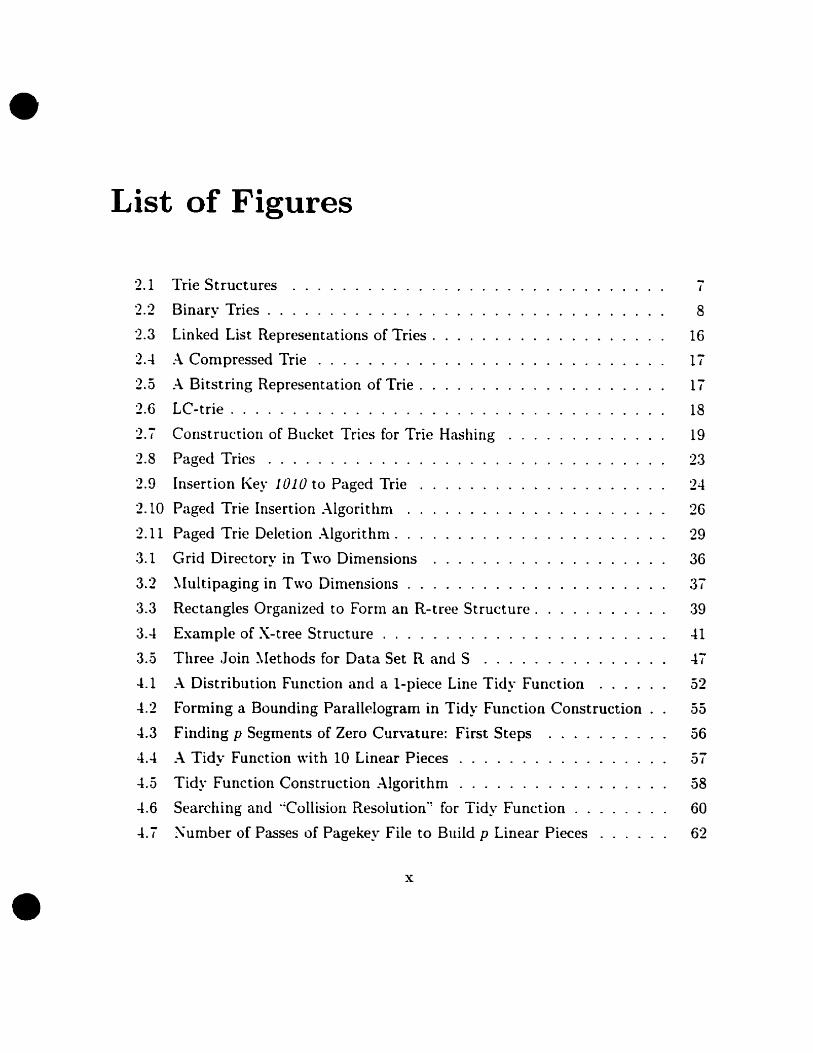
•List of Figures
•
2.1
2.2
2.3
2.4
2.6.) -_.1
2.8
2.9
2.10
2.11
3.1
3.2
3.3
3.4
3.5
·1.1
-1.2
-1.3
4.4
-l.5
·l.6
-l.T
Trie Structures
8inary Tries . .
Linked List Representations of Tries.
A Compressed Trie .
A Bitstring Representation of Trie.
Le-trie .
Construction of Bucket Tries for Trie Hashing
Paged Tries . . . . . . . . . . . .
Insertion Key 1010 to Paged Trie
Paged Trie Insertion Algorithm .
Paged Trie Deletion Algorithm. .
Grid Directory in T",o Dimensions
~Iultipaging in Two Dimensions . .
Rectangles Organized to Form an R-tree Structure.
Example of X-tree Structure . . . . . . . . . . . . .
Three Join ~Iethods for Data Set Rand S .....
A Distribution Function and a I-piece Line Tidy Function
Forming a Bounding Parallelogram in Tidy Function Construction
Finding p Segments of Zero Curvature: First Steps
A Tidy Function with 10 Linear Pieces
Tidy Function Construction Algorithm
Searching and '~Collision Resolution~l for Tidy Function
Number of Passes of Pagekey File to Build p Lincar Pieces
x
8
16
17
17
18
19
23
24
26
29
36
37
39
-lI
-l7
56
57
58
60
62

•
•
4.8
5.1-.)l>._
6.1
6.2
6.3
6A
6.5
6.6
6.7
6.8
6.9
6.10
6.11
6.12
6.13
6.14
6.15
6.lG
6.17
6.18
6.19
6.20
6.21
6.22
7.1- ,)1._
7.3
7A
Average Probes per Search versus File Size .
Trie Compression vs. File Size .
:\verage Number of Probes per Search \·s. Number of Data Records
Variable Resolution in Two Dimensions .
Exact :\!Iatch Queries by DyOrTrie
Range Query of [2,6)x[-l,8) in an 8x8 Space
Orthogonal Range Query using DyOrTrie .
Orthogonal Range Query using Grid File or ~Iultipaging
Page Searching in Orthogonal Range Query using ~Iultipaging
Page .-\ccesses vs. File Size, 20, Exact ~Iatch
Page :\ccesses vs. File Size, 160, Exact :\[atch .
Equivalent .-\ccess Times vs. File Size. 160, Exact ~[atch
Page :\ccesses vs. File Size, 20, Range Query
Page :\ccesses vs. File Size. 160, Range Query .
Equivalent :\ccess Times vs. File Size. 160. Range Query .
Page :\ccesses vs. Selecti\'ity, 2D
Page .-\ccesscs vs. Selectivity, 160 .
Equivalent :\ccess Tirnes vs. Selectivity, 1GD
Exact ~Iatch: Page :\ccesses vs. Dimension
Exact ~Iatch: .-\ccess Tinle vs. Dimension
Range Query: Page Accesses vs. Dimension
Range Query: .-\ccess Times vs. Dinlension .
Storage Cost vs. Distribution
Exact ~\'Iatch: .-\ccess Cost vs. Distribution .
Trie Compression vs. Record Size (Dinlension)
Joining Data Set Rand S by Tries
Xatural Join .-\lgorithm by Tries .
Disk .-\ccesses versus Join Selectivity
Disk .-\ccesses versus File Size
xi
64
68
69
71
73
i5
76
ii
79
82
82
83
85
86
87
88
89
90
91
91
92
92
93
94
96
100
103
110
111

•
•
Chapter 1
Introduction
1.1 Motivation
Space and speed are t\Vo major considerations for storage and retrieval in large
database systems on secc~dary storage. Furthermore. data. types and distributions
\"ary from application to application. There are special data such as text, spatial
(\'ector) and image (pixel) data versus structured data such as payrolls and invento
ries: one dimensional versus multiple dimensional data: order-preserved data versus
random-ordered data: uniformly versus non-uniformly distributed data; etc. Query
selectivities performed on data also vary from one application to another~ ranging
fron1 only one data item (record) to a significant percentage of source data files.
Query operations can be unary or binary as weIl.
An10ng the various existing data structures for large database systems~ a data
structure that is good at structured data may become inefficient if it is applied ta
spatial or text data. A data structure that behaves quite weIl for uniform data may
become inefficient for pathological data distributions. Data structures for organizing
one dimensional keys may not work for keys with multi-dimensional attributes. Fur
thermore~ data structures that support low selectivity queries nlay not be efficient in
performing high selectivity queries.
Hashing in general is good at single retrieval only. B-trees [B~'172] on secondaI')'
1

CHAPTER 1. IJVTRODUCTI01V 2
.'
•
storage have logarithmic behavior. K-D-B-trees (RobBI] extend B-trees for multidi
mensional data. Their costs of accessing secondary storage depend on the height of
trees~ and thus the fan-out, as weil as the data set size. The storage efficiency of grid
files [~HS84L a multikey direct access method~ is reduced by pûorly distributed data.
The access or storage efficiency of multipaging (~108Ia, ~1082] also decreases for
pathological data distributions. Bang-files (Fre87] and the Interpolation Based Grid
Files [0~192] use logarithmic accessing cost to compensate for the storage overhead
of grid files for nonuniform data. R-trees [Gut84] and their variants [BKSS90, SR87]
for spatial data contain overlapped hyper-rectangular regions which may lead ta less
efficient searehes for sorne queries than others. In addition, aU the aboye structures
do not generally support text indexing and searching.
In sunlmary. a data structure that is good at dealing with one kind of data in one
particular area for one type of query is likely to have bad performance for another
purpose. Is there a simple but powerful dynanlÎc structure for large-scale databases
that is efficient for text. spatial and structured data~ in terniS of both space and
speed; regardless of the distribution, the dimensionality. the operations, and the
query seleetivity?
On the other hand. digital trees [Knu73]~ or tries [Bri59. FreGOL are tree structures
that store data along paths rather than at nodes~ which is what a tree structure usually
cioes. They have many desirable eharacteristics. Among them~ the following three
are the most important.
1. They store data according to resolution. with the most important bits stored
near the root. Thus, we eaIl tries variable resolution structures or zoom tries.
Sueh a zooming property of tries may speed up queries at different resolutions
by starting with an approximation and refining it only when there is uncertainty.
Tries have been applied to various spatial queries and map retrieving. However,
it should be noted that the data need not to be spatial.
2. Tries compress data br requiring minimal storage overhead, only a couple of
bits per node. Paths near the root are shared by many data. In text searching,
such compression is important for indexing substrings in a large text~ which
requires at least a pointer to each character in the text .

CH.-\PTER 1. INTRODUCTI01V 3
•
•
3. Tries maintain order preservation in data. one of the fundamentals for efficient
high selectivity queries.
Tries, simple yet powerful structures. have shown advantages in nlany application
areas. In database systems they have achieved great performance in dealing \Vith text
data for \\'hich the trie compression makes substring indexing possible, which would
otherwise be impractical. \Vith spatial data, in addition to the storage advantage.
tries provide a way to do variable resolution queries in sublinear time.
But are tries aiso strong at organizing structured data such as tables and rela
tions? Are they efficient structures for both la\\' selectivity (such as exact matches)
and high selecti\"ity (such as range queries)? Can general relational algebra, such
as the join operations of relational databases be perfornled by tries efficiently, and
how? If yeso what are the advantages of applying trie structures to general database
systenls conlpared with state-of-the-act data structures and algorithms'? As far as we
know. these renlain open questions. This thesis attempts to answer these questions
by extending trie methods to be dynamic and applying various unary and binary
operations on structured data. and thus pursues the c1ainl that tries offer the best
general representations for large-scale databases.
1.2 Originality
To the best knowledge of the author. the originality of this work includes the following
methods. algorithms. comparisons and corresponding experimental results:
• DyOr·Trie. an extended pointerless bitstring representation for binaI)" tries used
for dynamic operations:
• .-\ piece-wise, linear tidy function approximation method with minimum over
flows. inc1uding construction and search algorithms for one-dimensional (ID)
queries:
• Comparisons of tries versus the tidy functions for 10 queries;

CH.-\PTER 1. INTRODUCTI01V 4
• • A new analysis of multidimensional data distribution for sorne direct access
methods based on information theory;
• Experimental comparisons of tries versus various direct and logarithmic access
methods for multidirnensional unary queries, including exact match and range
queries:
• Relational join algorithms by tries on structured data (binary operations on
tries):
• Comparisons of trie join algorithrns versus traditional and state-of-the-art join
algorithms.
1.3 Glossary of Symbols
Here are symbols used through the thesis.
N:
n:
P:
1..-.
p:
D(x):
B:
1.4
number of keys or records in a file on secondary storage
number of pages (blacks) in a file on secondary storage
page capaci ty
number of dimensions
number of linear pieces for tidy functions
cumulative distribution function
memory buffer size
Thesis Outline
•
The thesis is organized as follows. Chapter 1 presents motivation for the work and
the problem domain, followed by a summary of new results.
Chapters 2 and 3 principally concentrate on a literature review of data structures
and algorithms.
Chapter 2 concerns itself with trie structures. It reviews their properties, applica
tions. representations and sorne refinernents. The last section of the chapter presents

CHA.PTER 1. INTRODUCTION 5
•
•
an original dynarnic trie structure. This dynarnic trie is the underlying structure
which is used throughout the thesis.
Conventional data structures and joïn algorithms are introduced in chapter 3. It
reviews the data structures according ta their dirnensionality, from one-dimension
(10) to multidimensions. The ID structures include hashing and order preserving
key-to-address transfornlations. ~Iultidirnensional file structures are classified into
direct access and logarithrnic access files. :\ sun-ey of join algorithrn is also presented
in this chapter.
The rernaining chapters elucidate original work. They are organized in four chap
ters.
Chapter -l introduces a heuristic piece-wise linear approximation tidy function on
secondary storage. \Ve show its superiority to its closest competitors - sorne order
preserving hashing nlethods.
Chapters 5 ta 7 present three trie applications.
Chapter 5 dernonstrates tries for ID queries, conlparing with the piece-wise linear
tidy function that we propose in the previous chapter. Detailed comparisons on
storage and search cost are given.
Chapter 6 describes tries for multidimensional queries, comparing with grid files,
multipaging, R*-trees and X-trees. Exact nlutch and range query algorithms are pro
vided. as well as detailed experimental camparison results and discussions on speed
and space cost versus file size, record size, query selectivity, dimensionality, and dis
tribution. The results indicate that tries are better than other data structures when
files contain more than a few records and the query returlls more than a few records.
Chapter 7 demonstrates ho\\" tries can be used for binary join operations. ~atural
join and union join algorithrns are presented. \Vhen join attributes are organized by
tries, we show their significant advantage over all other join algorithms based on bath
theoretical analysis and experimentations.
Chapter 8 summarizes the thesis and proposes sorne future research tapies.

•
•
Chapter 2
Trie Structures
2.1 Trie lVlethods
The trie uses characters, or digital decomposition of a key, ta direct the branch
ing [Gongl]. The decision which way ta follow during a search from an internaI node
at depth d is made according ta the value of the dth position in the search key. For ex
arnple. a. trie for a key set of table, space. speed, trie and text is shawn in Figure 2.1(a).
The first letter splits the keys into two sets of subtries, s-keys and t-keys. The second
letter splits the t-keys into three groups of ta-keys, te-keys and tr-keys and so on.
\Vhen searching a ward, say trie, the first letter t leads us to the right child of the
root. The second letter r leads us ta the rightmost descendant. Eventually, if a leaf
node is reached. as in our case, a search returns successfully. Othenvise if a nulllink
is reached. it means the ward is not on the trie. Thus an unsuccessful search usually
stops at an internai node.
The trie presented in Figure 2.1(a) is referred to as a full trie [CS77] or pU1'e
trie [Ore82b]. ~ote that there exist subtries leading ta only one key (leaf node) in
a full trie. Such subtries can be pruned and the resulting trie is called an ordinaïlJ
trie (radix search tTee~ pruned trie [Knu73, CS77] or in most of the literature. simply
trie [Gong1]). Figure 2.1(b) is an example of an ordinary trie. The truncated char
acters, ce~ ed~ ble, xt and ie can either be stored on leaf nodes or in a separate file
6

CH..\PTER 2. TRIE STRUCTURES 7
•(a) Full Trie (b) Ordinary Trie
Figure 2.1: Trie Structures
o
(c) Patricia Trie
•
pointed ta by these leaf nodes.
There still exists a single descendant node~ between link sand p for words space and
speed in Figure 2.1(bL which does not brandI a search to any new subtrie. Such node
chains can be further eliminated if on the first branching descendant node a number
is used to indicate its corresponding level, or the number of skips from its ancestor
node. Figure 2.1(c) shows the resulting trie. ~umbers on internaI nodes indicate the
number of skips from their parent nodes. Such tries, without single descendant nodes
are called Patricia tries [~Ior68, Knu73, N1F85b, Gong1] (Practical Algorithnl To
Retrie\'e lnfornlation Coded In .41phanumeric). Patricia tries are especially capable
of indexing \'ery long, variable length and even unbounded key strings. Thus they
are very useful in text searching (cf. section 2.3).
The tries in Figure 2.1 are n-ary tries. Tries can also be binary. A binary trie is
a binary tree in \\-hich the branching decision on each node depends on the current
bit of a binary search key: branching left if it is 0, else right. A binary trie can be
fonned on the binary string format of numerical or alphabetic keys. Figure 2.2 shows
the binary full trie, ordinary trie and Patricia trie of the numerical key set {a, l, 2,
3. 7. 12. 13}. The corresponding bitstring set is {OOOO, 0001, 0010, 0011, 0111, 1100,
110I}.
Tries were first developed by de la Briandais [Bri59] and E. H. Fredkin [Fre60].
The name trie cornes from the ward retrieval [Fre60]. They were used for prefix
searching by ~[orrison [~'lor68]. Intensive discussions about the structure can be
round in Knuth [Knu73] and many other data structure books_ Tries \Vere associated

CH..\PTER 2. TRIE STRUCTURES 8
•(a) Binary full trie
II1101ilOIlOIl Il 01 II00000000000000
(d) FuTrie rcprcsentation
(b) Binary ordinary trie
IIII 01Il OO{ Il} 10II II 11000000000000
(e) OrTrie representation
Figure 2.2: Binary Tries
o
(c) Binary partricia trie
1{OH}I{OH} 1{2}{IOI1{OH} O{2}{ III O{O}{} O{O}{}I{OH} l{O}{}O{OH} O{Ol{} O(Ol{} O{O}{ 1
(t) PaTrie represenlation
•
with digital searches. and thus are also called digital trees [Knu73]. Since then~ tries
have been applied extensively t0 various text indexing and searching.
Several trie pararneters are of great interest: trie depth, height and size. Trie depth
is defined as the average path length frorn the trie root to its leaves. It represents the
average cost of a sllccessful search. Trie height is the longest path from the trie root
to the leaves. It is indicative of the worst case search time. Ideally, it is advanta
geolls ta know depth distributions in order to llnderstand the behavior of tries~ such
as how balanced/skewed the trie is. Trie depth/height has a rich research history
since 1970s [Knu73~ Dev82~ Dev84. Pit85~ Szp88~ Szp90~ Szp91, .Jac91~ Dev87, Szp92.
Szp93~ RJS93. CFV98, CFV99, KSOOb, KSOOa]. Trie size in storage consumption
is as inlportant a parameter as trie depth and height in measuring access time. It
is the nurnber of nodes in a trie. Trie size has been analyzed and explored in the
literature [Knu73. Jac91. Szp90, Szp91, CFV98~ CFV99] ..-\ trie is called a symmetric
trie if data stored on tries are uniformly distributed. Otherwise, it is an asymmetric
trie. For asymmetric tries~ the entropy determines depth distribution. The more
asymmetric the symbol alphabet is, the more skewed a trie is. Sorne discussions of
asymptotic behavior of asymmetric tries can be found in the literature [RJS93, FL94.

CHA.PTER 2. TRIE STRUCTURES 9
•
•
KSOOa, KSOOb]. Since the late 1970s, prefix tries have also been applied to spatial
data index schemes ranging from quadtrees • [Hun78, Dye82, Sam90], octries [Nlea82],
k-d-ties [Ore82b], pr-ties [Sam90], and FuTries p~IIS94, Sha94]. The 1980s saw various
trie structures proposed for dynamic trie hashing. Other development and applica
tions of tries include lexical analyzers and eompilers. natural language analysis, data
compression, pattern recognition, parallel searching, and even Internet IP routing. :\
brief trie history can be found in .-\ppendix 1.
The next two sections will foeus more specifically on trie properties and applica
tions.
2.2 Trie Properties
The sinlple but elegant trie structure has many attractive properties, and thus has
been applied to various database and non-database applications.
• The compression of data by the overlap of paths near the root reduces space
cost of the trie, and provides faster transfer of data from the seeondary storage
to t he main memory.
• It stores the nlost significant bits first near the root. It allows queries to start
at sorne approximation and perform refinernents by reading lower levels of tries
only if there is uncertainty.
• Tries are arder preserving data structures which is essential ta high selectivity
queries such as range queries.
• Prefix searching looks for any word that matches a given prefix. Trie searching
is. in fact. prefix searching, unlike hashing or any other normal tree search.
Patricia tries are capable of indexing extremely long and unbounded keys and
thus are extremely suitable for prefix searehing.
•{;nÎortunately, the ternI quadtree is confusing as it has different meanings. In most cases, itrefers to a trie structure and thus should be called quadtrie. In sorne ather cases, it may also referta a tree structure (FB7-l. FGP~193, FL9-l] .

CH.-\PTER 2. TRIE STRUCTURES 10
•
•
• The shape of the trie is uniquely determined by the data sets, and thus is not
affected by poor data distributions.
• Tries can be interpreted as multiple key structures and hence are amendable to
multidimensional space. A key with multiple attributes can first be interleaved
bit by bit to an interleaved key. Then these interleaved keys can be used to
construct a trie. as if they were in one dimension.
• Tries have short search time. Successful search cost is bounded by the length
of the search key, regardless of the file size. Unsuccessful searches may cost less
as they are likely to stop at internaI nodes.
• Trie structures are flexible and can be combined \Vith many other structures sim
ply by applying the trie structure near the root and switching to these structures
near the leayes. Further explanations are discussed in the next section.
2.3 Trie Applications
2.3.1 Prefix searching
~'[any applications require recognition of keywords from dictionaries and thus require
efficient prefix searching. Traditional dictionary lookups, such as hashing and tree
searching, do not support search keys to be prefixed or abbreviated and thus are
inadequate. Trie structures, on the other hand, are ideal for indexing prefixes. Trie
searching has been applied for data compression [B\VC89, BK93], lexical analyzers
and compilers [ASU86), pattern recognition [B589, DTK91, ABV95], spelling checkers
(LE~[R89L natural language analysis [TITK88, Jon89], parallel searcbing [HCE91]
and Internet routing [NK98].
2.3.2 Text Searching
A major problem for text indexing which is capable of accessing every substring of
a large text is its size. Clearly, at least one pointer is needed for every character in

CH.-\PTER 2. TRlE STRUCTURES Il
•
•
the text and each pointer is at least logJV bits. where lV is the number of substrings.
The total index must be of size J,V log JV bits or ~ ~V log lV bytes. For a text of size 227
characters or substrings such as the New Oxford English Dictionary (OEDJ, pointers
to the text already require 3A1V bytes. Trie compression mal--es text indexes possible.
Along with its capability to index very long and even unbounded strings and its fast
access property. the trie is a suitable data structure for text indexing and searching.
• prefix search:
Tries have been used for prefix searches by ~Iorrison [~Ior68] and exploited by
Gonnet et al. [Gon88~ GB\rgl. Tom92] as the basis for the retrieval methods
used in the electronic version of the New üED. using P.-\T tries.
Gonnet [Gon88] treats a text as a long single character string. A sistring is a
semi-infinite suffix of a text. A trie of string suffixes is a suffix trie [Apo85,
Szp92]. E\'ery subtrie of a suffix trie has aIl the sistrings of the given prefix.
Prefix searching in suffix tries consists of searching tries up to the point the
prefix is exhausted. or when there are no more subtries. In either case the
search cost is only bounded by the length of the prefix, independent of trie size.
Suffix tries are efficient for prefix searching and longest repetition searching.
• longest repetition search:
Longest repetition of a text is a match between two sistrings which has the
most number of characters in the entire text. For PAT tries, it is the sistring
pair with the highest depth. For a given text, it can be found during the
construction of the trie. It can be applied to manipulations of general sequences
of symbols [SK83L such as string editing, comparison, correction and collation
of different versions of the same file. It is also applicable to genetic/biomedical
sequences.
• range search:
Suffix tries or PAT tries can do range search efficiently, searching for all the
strings that are lexically between two gi\'en values, in the order of trie height
[Gon91] and the size of the answer set .

CH.4PTER 2. TRIE STRUCTURES 12
•
•
• most frequent search:
This search is to find the most frequently used string in the text. \Vith suffix
tries. it is equivalent to finding the largest subtrie whose search path begins
with a space and ends with a second space [Gon9!]. This type of search has
great practical interest such as finding the most frequently used word in a text.
• regular expression search [B'YG89]:
Regular expression searching also has great practical interest. Tries have been
also applied to regular expression searches of texts [BYG89~ Gon91~ Sha94].
• proximity search:
This search gives strings that are at a fixed distance away from a given string.
The distance of two strings can be defined as the nurnber of differences (in
sertion. deletion. substitution and/or transportation) between the t\Va given
strings. '"arious data structures. algorithms and techniques have been devel
oped and applied to solve this problem [Knu73! HD80. SK83~ Kuk92~ BYP92] .
.-\gain. tries are one of the structures that can he readily applied to it. In
Gonne(s paper [GBY91L PAT array, a compact representation of the PAT
tree. was used for proximity searching. Shang and ~Ierrett [Sha94, S~I96] apply
Fu Trie. a binary full trie structure. to proximity searching.
2.3.3 Spatial Data Representation
Spatial data are points. lines. etc. in multidimensional space. Prefix tries for spatial
data are tries on interleaved numerical data. with the most significant bits stored
close to the trie root. This variable-resolution structure allows sorne queries to look
only part way clown the trie to retrieve and search on approximations. The search
choice on anode can be ··accept'~ (all records in the subtrie are in the answer setL
or "reject" (no record in the subtrie is in the ans\ver set): or ;';'explore", wben tbere is
uncertainty at this early stage. The search only goes clown to subtries wben there is
uncertainty.
CHA.PTER 2. TRIE STRUCTURES 13
•
•
Tries have been applied to spatial data indexing schernes, rangÏng from k-d
tries (Ore82b], octrees [Nlea82], pr-tries (Sam90], zoom tries (~IS94] to various quadtrees
(quadtries) [Hun78, Sarn90]. Sorne of the other multi-dimensional structures such as
k-d-trees~ K-D-B-trees, gnd files~ muLtipaging, R-trees etc. will be discussed later in
chapter 3.
K-d-tries are a generalization of 10 binary tries. They are named after k-d
trees [Ben75], because they use the same principle of interleaving coordinates. The
advantage of k-d-tries over k-d-trees is that tries store data under variable resolutions,
i.e .. the nlost significant bits are stored near the root. This property, zooming, \Vas
exploited to display spatial data at any reso1ution using on1y one copy of the data
and transferring from secondary storage only the amount of data needed for that
display [~IS94. Sha94].
2.3.4 Other Applications
Signal Processing and Telecommunications
One of the most inlportant issues in signal processing is to e3timate the output for a
known inpuL Le.. a query from the input/output data seen to this point. A nonlinear
adaptive estimation method that uses a k-d-trie was presented in [Iig95]. 1V records
of k-dinlensional input vectors and their corresponding scalar outputs are stored in
the k-d-trie. These latest ~V input/output records are used to estimate the output of
a given input (query point). A trie range search. with ma.ximum distance from the
query point in each dimension less than L, is perfornled. Then, a non-linear local
model is applied to those records retrieved from the range query in order to obtain
the estimate of the output. The method requires updating the trie as each new data
point is available such that only the latest ~V data are maintained on the trie. The
k-d-trie is chosen instead of a k-d-tree since it has superior performance to the latter
in terrns of the average time requirement for updating; it requires no rebalancing
operations for insertions and deletions.
Data compression. message encoding/decoding techniques are widely used in telecom
munications. Ziv-Lempel (ZL77, ZL78] coding is currently one of the most practical
CH.4PTER 2. TRIE STRUCTURES 14
• data compression schemes. It operates by replacing a substring of a text \Vith a
pointer ta its previous occurrence in the input. Tries are one of the structures capa
ble of longest string searching as mentioned above [BK93].
~Iessage decoding and conflict resolution algorithms for broadcast cornmunications
can also be equi\'alent to trie search processes [Cap79, Ber84, ~IF85a].
Image processing
Trie hashing has been used as a dynamic method for similarity retrieval in picto
rial database systems. It is claimed to have good perfornlance in pictorial database
management systems [CL93].
2.4 Trie Representations and Aigorithms
2.4.1 Tabular Forms
Tries have been represented variously. :\. straightforward implementation is the table
or matrix form [Fre60~ :\lor68. Knu73, RBK89]. :\. k-ary trie with S nodes and lV
keys is represented by a table of k x (S - 1V) entries. where k is the number of rows
and S - .V the number of colunlns. In the table~ each column represents an internai
node of the trie, where each table entry contains a colunln number, a null pointer,
or a pointer to a key (leaf node). The first column is the root. Table 2.1 gives the
tabular format of the binary trie given in Figure 2.2(a). There are 20 table entries
for.V = 7,k = 2. and S = 17.
o1
a 1 2 3 4 5 6 7 8 91 2 9 0010 6 1100 00004 7 3 0011 5 1101 8 0111 0001
•
Table 2.1: Tabular Format of a Binary Trie
Civen a key, the search is initiated by looking up the table starting at the first
column~ the root node. If following the column number of a link, an empty entry is

CHA.PTER 2. TRIE STRUCTURES 15
•
•
found, the search returns unsuccessfully. :\. search is successful if a termination con
dition (a leaf node) is reached and matches with the search key. Dynamic insertion
of anode simply amounts to adding a new eolumn and putting a eolumn number at
the entry of its parent column. In faet, Table 2.1 is the result of dynamic insertions
of the keys in the following order: {DOlO, 0011, 1100, 1101,0111,0000, OOOl}. Dele
tions may leave blank columns in the table which may be filled by the last column.
However! the parent node of the last column must be updated too. ~lerrett and
Fayerman [~IF85bl suggest locating the parent column by adding reverse pointers to
each node. Shang [Sha94] suggests that it can be solved without adding extra storage
o\'erhead. Instead, simply seareh for a keyword clown the subtrie rooted at the last
column followed by another search of the keyword from the root.
There are more subtle implementations of the tabular forms by either using three
arrays or double arrays to minimize the storage overhead [TYt9. :\.oe89]. The idea is
to compress the table iota a ID array with fe\ver entries by mapping from positions
in the table to the array such that no two non-empty entries in the table are mapped
ta the same position in the array.
2.4.2 Linked Lists
Tabular representations are prohibitive when k is large for a k-ary trie when many
of the entries in the table are empty. Dynamic structures, such as linked lists, are
an alternative way ta overcome the problem (ES63, Knu73, AHU83. Jon89, Dun91].
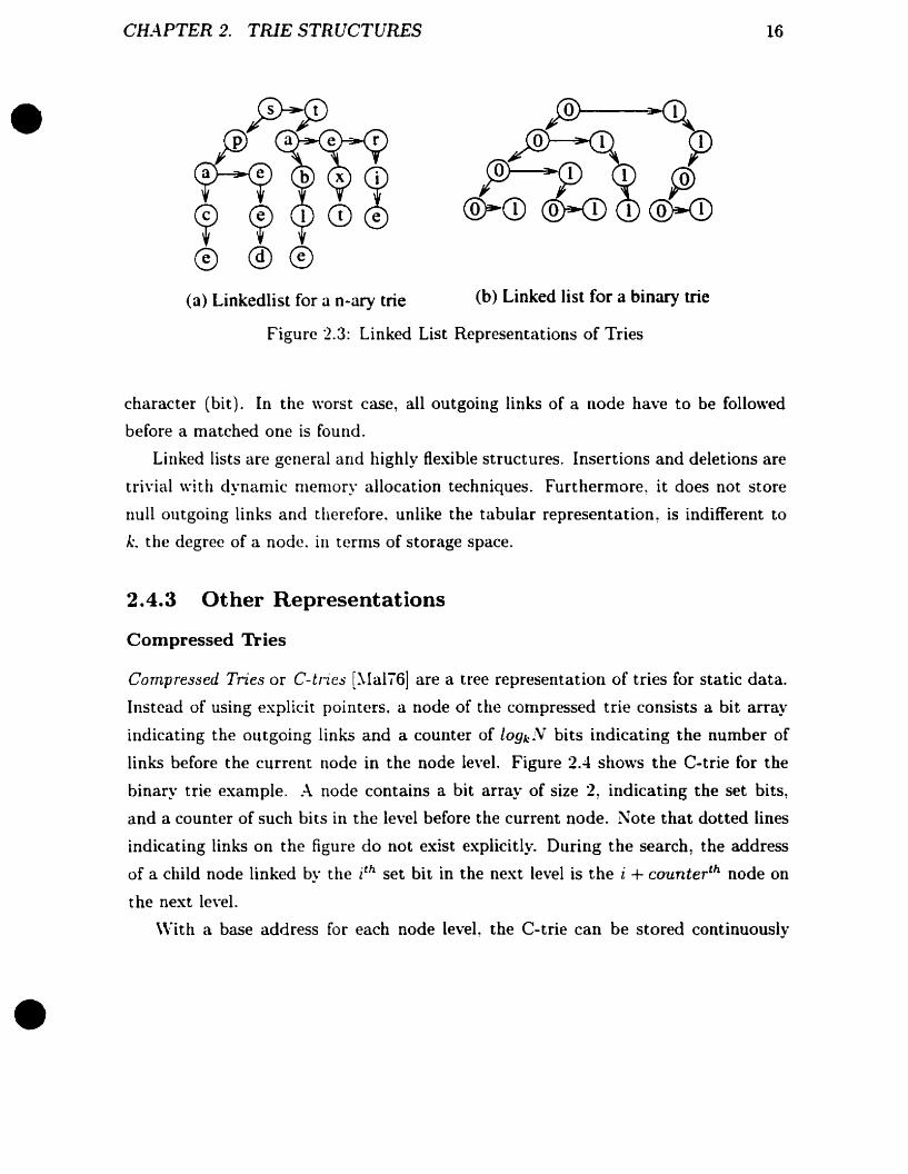
Figure 2.3 shows the corresponding linked list representations of the alphabetical and
the numerical trie exanlples.
In the linked list representation, each node is a linked list of outgoing (right) links.
The link contains a character and a pointer to the left-most child in the siblings of
the child node (left link). This is in fact a dO'uble chained tree [ES63], or a binary tree
[Knuï3].
Searching on anode is done by comparison of a character (bit) of the key and
the character (bit) on the node~ following the outgoing (right) links until a match is
round: then the pointer to the left-most child (left link) is taken to match the next
•CH.4PTER 2. TRIE STRUCTURES
(a) Linkedlist for a n-ary trie (b) Linked list for a binary trie
16
•
Figure 2.3: Linked List Representations of Tries
character (bit). In the \Vorst case, ail outgoing links of a node have to be followed
before a matched one is round.
Linked lists are general and highly flexible structures. Insertions and deletions are
trivial with dynamic menlory allocation techniques. Furthermore, it does not store
null olltgoing links and therefore. unlike the tabular representation, is indifferent to
k. the degree of a node. in ternlS of storage space.
2.4.3 Other Representations
Compressed Tries
Compressed Tries or C-tries [~Ialï6] are a tree representation of tries for static data.
Instead of using explicit pointers. a node of the compressed trie consists a bit array
indicating the outgoing links and a counter of [09k1V bits indicating the number of
links before the current node in the node level. Figure 2.4 shows the C-trie for the
binary trie example. :\ node contains a bit array of size 2! indicating the set bits,
and a counter of such bits in the level before the current node. Note that dotted Hnes
indicating links on the figure do not exist explicitly. During the search, the address
of a child node linked by the i th set bit in the next level is the i + co'unterth node on
the next level.
\Vith a base address for each node level, the C-trie can be stored continuously

•CH.4PTER 2. TRIE STRUCTURES
[iliJ.o
8n 0 [ili] 2
ŒE1.0 [ili] 2 [ili] 2
[ili] 0 [ill2 rn -l
~ 0 [ili] 0 [ili] 0 [ili]0 ~ 0 [ili] 0
Figure 2.4: A Compressed Trie
17
•
on secondary storage level by level, and node by node within each level. It is a very
compact representation for static data.
Bitstring Representations
8itstring [Ore82a~ Ore82b) extends the C-trie even further by only storing bit arrays.
Finding the child link on the next level involves Hnear scanning on the next level.
.-\. bitstring representation of the binary trie example is given in Figure 2.5. The
bitstring in curly brackets indicates the remaining bits of the leaf. But Orenstein
argues that the Humber of bits scanned in each level cao be reduced to an arbitral')'
constant by organizing bits into blocks depending on the black size.
1111 0111 00{11} la11 11 1100 00 00 00 00 00 00
Figure 2.5: A Bitstring Representation of Trie
Bath C-tries and bitstring representations are pointerless trie structures.

CH.-\PTER 2. TRIE STRUCTURES 18
• 2.5 Trie Refinements
•
2.5.1 Le-tries
Le-trie [.\~93] applies LeveL compression to reduce further the height of the patricia
trie. The basic idea is that if the i th highest level of a trie is complete, but level (i + 1)
is not. then the ith highest levels are replaced by a single node of degree ki (2 l for a
binary trie). The replacenlent is applied top-down starting from the root. Figure 2.6
shows the LC-trie transfered from the patricia trie in Figure 2.2(c).
Figure 2.6: Le-trie
It is claimed by .\ndersson [.-\~93] that for random~ independent data~ the average
depth of a LC-trie is reduced to 8(log· ~V) from o (log lV), where ~V is the nunlber of
keys.
2.5.2 Hybrid Tries and Trie Hashing
Because of the flexibility of trie structures, they are often combined with sorne other
structures to obtain efficient behavior, i.e., applying trie structures near the foot and
switching to other data structures near the leaves. They are referred to as hybrid
tries. One cornmon combination is \Vith external buckets, called bucket tries [Knu73].
Bucket tries are widely used as collision resolution strategy for dynamic trie hash
ing [ED80, Lit8L Lit85. LZL88. LRLH91] .

•CH.-\PTER 2. TRIE STRUCTURES
internai oode bucket buckclS
~0~'"inœm31 node
~ ~ IS~cd IEJ ~space spac;e
0 0 1 0
lJI (bl
19
buckets
I::~ Il ~~~e 1EJo 1 l
internai node(sl
~~~o 1 :!
•
(Cl
Figure 2.7: Construction of Bucket Tries for Trie Hashing
Suppose keys in Figure 2.1 are inserted in the follo\Ving order: {table, space, speed,
trie. text} and the capacity of a bucket is two items. Figure 2.7 shows the dynamic
construction of the bucket trie for hashing. A trie node contains four fields: DV, DN,
LP and HP. where DY is the value of the digit, DN the digit number of the key, and
LP and CP are two lower and upper pointers, either to internai nodes or external
buckets. The value of an internal pointer is anode address. The value of an external
pointer is either the address of a bucket or null. In arder ta distinguish internaI and
external pointers. the value of an internai node is in fact the negative of the node
address. In Figure 2.7(a). when the first t\Vo keys are inserted, they are stored in
bucket O. No internai nodes are needed. Figure 2.7(b) shows that when speed is
inserted, bucket 0 contains three keys. and thus has ta he split iota t\Vo at the first
digit s. Any key with the first digit greater than s is stored in bucket 1 and painted
ta by the HP pointer: othenvise it is in hucket 0 and pointed ta by the LP pointer.
The branching information is stored in an internai Dode O. Figure 2.7(c) shows the
insertion of the last key. Bucket 1 containing table, trie, text is split iDto hucket 1
aDd 2 at the first two digits te. Correspondingiy, t\Vo internai nodes are generated,
\Vith Dode 1 for the split at the first digit t and Dode 2 for the second digit e.
CH6-\PTER 2. TRIE STRUCTURES 20
.' Trie hashing has been claimed to require one disk access when internaL nodes of
the trie can be heLd in RA~I ~ and two accesses for very Large files when the trie has
to be on disk [Lit85~ LZL88. LRLH91]. Furthermore, the file can be highLy dynamic.
2.5.3 FuTrie, OrTrie and PaTrie on Secondary Storage
Fu Trie. OrTrie and Pa Trie are three pointerless trie structures. FuTries. OrTries
and PaTries denote the binary full tries, binary ordinary tries and binary patricia
tries [Sha9.t] respectively. The three organizations are extensions of Orenstein!s point
erless bitstring representations on secondary storage. They use two bits for each node
and tries are partitioned inta pages. and thus are suitable for secondary storage.
FuTrie
FuTrie is a binary tree whose nodes do not store information and whose left links arc
labelled with 'O's and right links with 'l·s. The ith bit of a search key determines the
link to be followed at lever i of the trie: if it is '0' ~ go Left and otherwise right. ThllS.
each root-to-leaf path has il one-to-one correspondence to a key. The height of the
trie is bounded by the length of the keys.
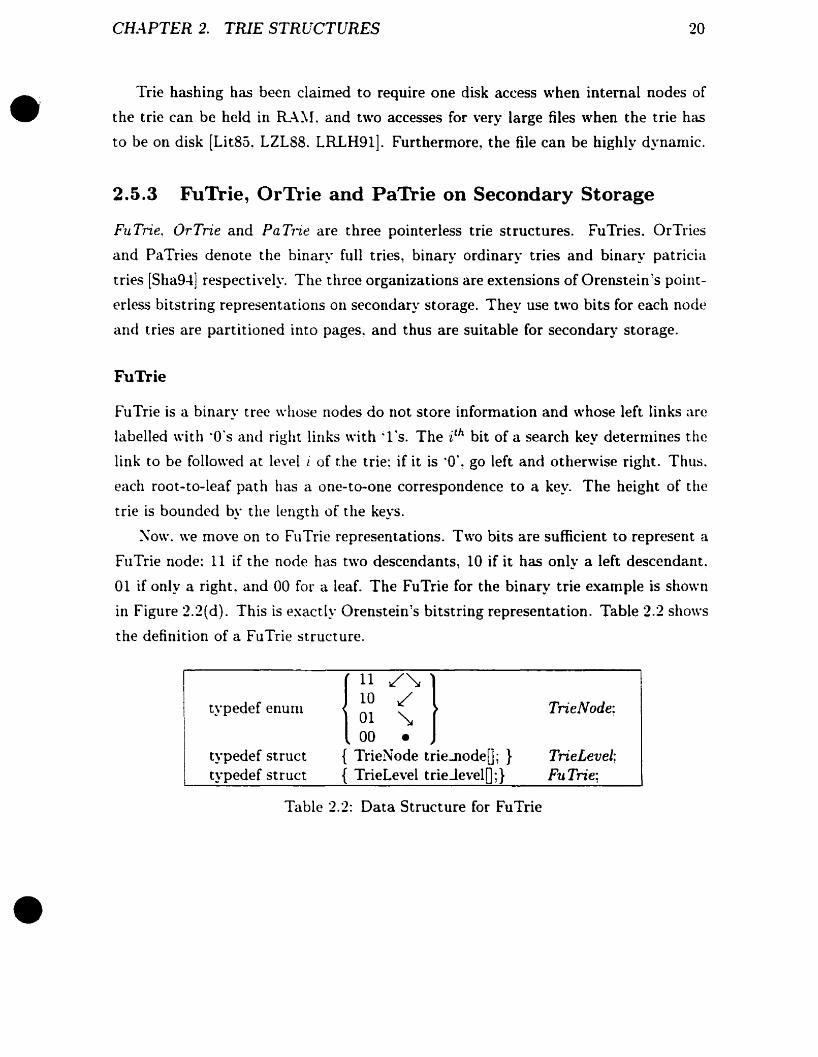
:'\ow. we move on ta FuTrie representations. Two bits are sufficient ta represent a
FllTrie node: Il if the node has two descendants! 10 if it has only a left descendanL
01 if only a righL and 00 for il leaf. The FuTrie for the binary trie example is shawn
in Figure 2.2(d). This is exactly Orenstein's bitstring representation. TabLe 2.2 shows
the definition of a FuTrie structure.
typedef enunI
typedef structtypedef struct
III /~)la /01 ~
00 •{ TrieNode trie..nodeD; }{ TrieLevel trieJevel0;}
TrieNode;
TrieLevel;Fu Trie;
•Table 2.2: Data Structure for FuTrie

CH.-\PTER 2. TRIE STRUCTURES 21
• OrTrie
An OrTrie is a pruned FuTrie in which subtries containing only one leaf are pruned.
Figure 2.2(e) shows the OrTrie transformed from Figure 2.2(d), Bits in curly brackets
are the path-to..leaf suffices that have been truncated. It can also be a pointer to the
corresponding key or record stored in an external file. The OrTrie structure is defined
in table 2.3.
typedef enUffi
typedef structtypedef struct
PaTrie
Il1001
{{sujJix} {other_attributes} }
00 or{pointer}{ TrieXode trie-IlodeO; }{ TrieLevel trieJeveID;}
Table 2.3: Data Structure for OrTrie
•Trie!\iode:
TrieLevel:Or'Trie:
PaTries are used ta represent binary patricia tries. Figure 2.2(f) shows the PaTrie
representing the patricia trie in Figure 2.2(c). As there are no single descendant nodes
in a binary patricia trie. a node on a PaTrie can be represented br one bic 1 for an
internaI node and a for a leaf node. For an internai node. the number of skips and
the corresponding substring that has been skipped need only be attached. For a leaf
node, either a pointer ta the record or suffix of the key and other attributes of the
record have to be stored. Table 2...l shows such a PaTrie structure.
typedef enum
typedef structtypedef struct
{
1{#skips}{ substring}
a{ {length}{suj jix} }or{pointer}
{ Trie~ode trieJ1odeD; }{ TrieLe\"el trieJeveID;}
TrieNode;
TrieLevel;PaTrie;
•Table 2.-1: Data Structure for PaTrie

CHA.PTER 2. TRIE STRUCTURES
Paged Tries
22
•
.-\s it stands~ like the C-trie and the bitstring representation, FuTrie, OrTrie and
PaTrie structures require a sequential search on each trie level, destroying the laga
rithrnic search cast and the variable resolution advantage tries provide. However, in
a paged structure for secandary storage, this can be fixed.
The paged structure partitions a trie into layers (page levels) of l node lcvels each.
and then cuts each layer vcrtieally inta pages of subtries. \\ïthin a page. descendant
nades of each layer are either entirely on or entirely off the page, i.e., links ean only
cross the horizontal boundaries of layers, not the vertical boundaries of pages. The
resulting paged trie reads one page pel' layer from secondary storage during the search.
and restricts sequential search within pages only.
Figure 2.8(a) shows the paged OrTrie with l = 3 and a page capacity of three
nodes. .-\ page contains two counters to avoid the sequential search and redecnl the
trie search. Tco'Unt enunlerates the number of links entering the page le\'cl fronl the
abo\"e. up to but not induding the current page. Bcount does the same for links
leaving the bot tom of the page level. The two counters can be used to find the page
where the left descendant of the node ·'X·, locates without a sequential scan of pages
in the next page le\·el. The Beount of the page with node "X" is -1, which nleans
-l links have already descended from earlier left pages in the page level. As the left
descendant of "X" is the first link in the page, so it is the 5th leaving the current page
level. Thus in the next page le\·el. we must look for a page with Tcount the greatest
integer less than (or equal ta) 5. The candidate pages on the page level below are
Tcount= 0 and 3. and thus we choose 3. Thus the left descendant of '~X,· is located
on the second page in the next page level.
Thus far. when checking Tcounts at the next page leveL we still do a sequential
scanning. However. it can be avoided simply by moving Tcounts of each page le\"el up
into lists of Tcounts in the parent pages above. Theo we can calculate directly from
the current page which page ta follow on the next level. .-\S shown in Figure 2.8(b).
each page contains a Bcount and a list of Tcounts of child pages. Dashed lines painting
ta pages are implicit in the paged trie structure.

CH.4PTER 2. TRIE STRUCTURES
:······_··········...··(i·~~ Il lo.IA~ Il 01 i
'"·ïi·~~~::~::~:r~:::;~~--···7·.~O.3' Il 1 OO{ Il} 10 (3/~ IIII~II i
····.::::::::=:l'''~:~:::·::::;;:::[::::::~::f 7, 00 00 oof 00 00 00 ~f'~t. _ J )
23
(a) Paged OrTrie (b) Paged OrTrie Structure
Figure 2.8: Paged Tries
•
The paged OrTrie structure is given in Table 2.5.
typedef struct { int Tcount; }OrTriePage *page; } LinkTo;
typedef struct { int Bcount;LinkTo linktoD;OrTrie bitstrings; } OrTriePage:
typedcf struct { OrTriePage trie_page0;} PagedOrTrie:
Table 2.5: Data Structure for Paged OrTrie
2.6 DyOrTrie, a Refinement of the OrTrie for Dy
namic Data
This section describes new work~ although it appears in a review of trie structures. ft
is an irnprovement over the existing paged trie structures, OrTries, for dynamic data
insertions and deletions.
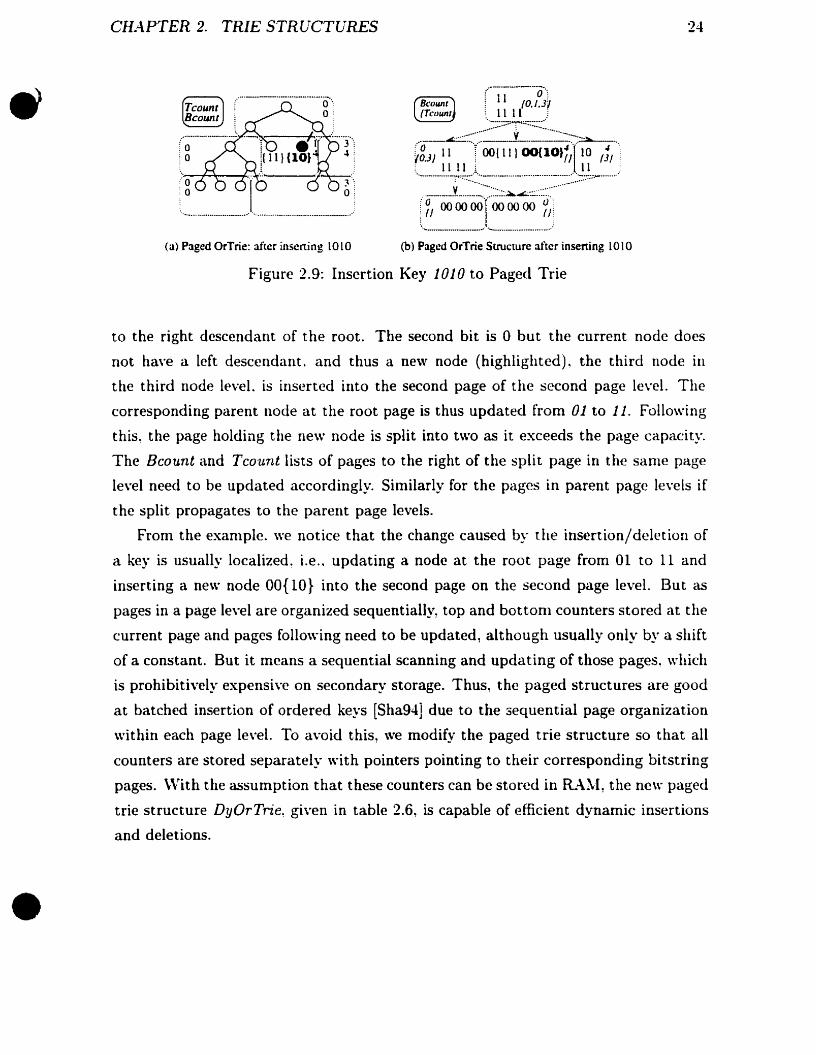
Insertion is straightfonvard for the paged OrTrie. An insertion of key 1010 to the
trie presented in Figure 2.8 is given in Figure 2.9.
The insertion fo11ows a search of the key. As the first bit is 1, the search goes
CHA,PTER 2. TRIE STRUCTURES
(a) Paged OrTrie: after inscrting 10 10
(l·ï-··-;.-;~·1: 1111 :
... ,",:~::~:::~:~~J~~~===-:.~~_ ..jg3' Il f DO( III OO(lOI1,'[ 10 fJ,': Il Il i Il '"~_.._.....' .._"':::::'-".__...._".""_.."'.._" ...._..~~~~~:..::::::.-.......
lF-oo.:~:(~~~_:~r-(b) Pagcd OrTrie Structure after inserting 1010
24
•
Figure 2.9: Insertion Key 1010 to Paged Trie
to the right descendant of the root. The second bit is 0 but the current node does
not have a lert descendant. and thus a new node (highlighted) ~ the third node in
the third node level. is inserted into the second page of the second page level. The
corresponding parent node at the root page is thus updated from 01 to 11. Following
this~ the page holding the new node is split into two as it exceeds the page capacity.
The Bcount and Tcou.nt lists of pages to the right of the split page in the same page
level need to be updated accordingly. Similarly for the pages in parent page levels if
the split propagates to the parent page levels.
From the exanlple. we notice that the change caused by the insertion/deletion of
a key is usually localized~ i.e .. updating anode at the root page from 01 to Il and
inserting a new node OO{ ID} into the second page on the second page level. But as
pages in a page level are organized sequentially, top and bottonl counters stored at the
current page and pages following need to be updated, although usually only by a shift
of a constant. But it means a sequential scanning and updating of those pages~ which
is prohibitively expensive on secondary storage. Thus~ the paged structures are good
at batched insertion of ordered keys [Sha94] due to the 3equential page organization
within each page level. To avoid this, we modify the paged trie structure so that all
counters are stored separately \Vith pointers pointing to their corresponding bitstring
pages. \Vith the assumption that these counters can be stored in RANI, the ne\\" paged
trie structure DyOrTrie~ given in table 2.6, is capable of efficient dynamic insertions
and deletions.

•
•
CHA.PTER 2. TRIE STRUCTURES
typedef struct { int Tcount; }OrTrie *page; } LinkTo;
typedef struct { int Bcount;OrTrie *page:LinkTo linktoO;} OrTrieLink;
typedef struct { OrTrie pageO;OrTrieLink linkD; } DyPagedOrTrie:
Table 2.6: Data Structure for Dynamic Pageti OrTrie
Insertion of a record starts \\'ith a search of the record. The search may result in
one of the following situations:
• .-\ lear node is found. and the remaining bits of the Hode nlatch with that of the
search key. This is a duplicate key and the insertion algorithm returns.
• The search stops at an internai node, because it can not find the branch aecord
ing to the seareh key. In this situation, update the eurrent node from DIor 10
to Il and add a corresponding descendant leaf node at the child level.
• The search stops at a leaf node. but the remaining bits of the node do not mateh
\Vith that of the key. In this case~ the originalleaf node that \Vas truneated has
ta be extended to the level at which the bit of the original key differs frOlTI that
of the new key.
The update in the second scenario is rather local. Cpdating the node from DIor
10 to Il costs no extra storage space. But adding a corresponding descendant leaf
node to the child level may occasionally cause the page where the child level is located
ta exceed page limits. and thus a page split is required. But the split does not in
any situation propagate ta upper levels. On the other hand~ the extension of links
in the third scenario may cause the pages on the path from the node to the leaves
exceed page Iimits and require splitting. Furthermore~ the split may propagate from
the page holding the two leaves ta the page where the node extension happens.
Figure 2.10 shows the pseudo-code for key insertions. Like B-trees: the cast is
bounded by the trie height due to the occasional splitting of trie pages whieh may

•CHAPTER 2. TRIE STRUCTURES
Boolean Trielnsertion(key){
Ilsearch the key and find the node that is either a Ieaf node orlIa node that the search has to stop because of a mismatch:node= search_and_find_nodeCkey);if (node -> is_Ieaf() kt node-> rest_bits_match_with( key» {
Ilthe key is already on the trie:return (false);
}
if (node-> is_Ieaf() li !node-> rest_bits_match_with( key» {Ilexpend the node until the two keys differ (return the new leaf):node= node-> expend(key);
}
else { Ilnode is not a leaf, at which the node is updated to 11 andlIa new leaf node is created at the next level:
new_Ieaf_node= node-> update_node_value();node= new_Ieaf_node;
}
Ilsplit the page if necessary:page= node-> current_page();while ( page != NULL ii page-> size() > page_capacity) {
if (page -> parent_page != NULL) { Il not root pagesplit_page ( page);Ilupdate page links and counters in the parent page level:page= page-> parent_page();page -> update_page_links_and_counters();
}
else Ilthis is root page, cannot be split:return (false);
}
}
void split_page( OrTrie .page){
26
•
Illinear scan of the page and find i'th subtrie at whichIlsubtries 1, ,i consumes <- page_capacity whileIlsubtries 1, ,i,i+l consumes> page_capacity:i- find_subtrie_in_page_by_Iinear_scan ( page);/Imove subtries i+l, ... from page to a newly constructed page, nevpage:OrTrie .newpage = new OrTrie(page, i+l);Ilupdate page links and counters of page and newpage:page->update_page_Iinks_and_counters();newpage-> update_page_Iinks_and_counters();
}
Figure 2.10: Paged Trie Insertion :\.lgorithm

•
•
CHA.PTER 2. TRIE STRUCTURES
propagate up to the root page.
Now we discuss the splitting algorithm and the page utilization after splitting.
\Vhen a trie page exceeds the page capacity during the insertion, the page is forced
to be broken into two pages. Ideally, we would like the two pages to be equally full.
Due to the fact that trie pages do not have branches to neighboring pages in the same
page level, the issue becomes dividing the page containing a forest of subtries into
t\Vo groups of subtries of approximately equal size. :\5 these subtries are ordered! the
splitting is to find the i th subtrie in a total of m 5ubtries 5uch that subtries 1. 2.....
and i consume no more than half of the page capacity. but if i+1 is included. they
exceed half of the page capacity. Thus, subtries 1,2, ... ,i renulÎn in the original page
and subtries i+1, ....Tn move to the newiy generated page. This can he done simply
by a linear scan of the page in R:\~·1.
The least page occupation after splitting occurs when the splitting houndary is
set at subtrie i + 1 which is a complete trie. ~Iore over, the least page utilization
\'êlille is a function of the page capacity P and the nurnber of node levels in a page!
l. :\ complete subtrie of 1 levels has 21 - 1 nodes and each node takes 2 bits! Le..
approxirnately 21+ l bits or 2l- 2 bytes for the subtrie. Sa the least page lltilization rate
is correspondingly 1/2 - 2l- 2 / P. Thus, the larger the page capacity Pis! the higher
the least page occupation is. On the other hand, the more node levels there are, the
lower the least page occupation can he. For instance. if the page capacity is -1096
bytes and there are 10 node levels in a page level. then the least page occupation rate
is 1/2 - 2 LO-
2 /-I096 = 0.-1375.
:\ deletion also starts with a search of the key. There are three different situations
as fo11ows.
• The search stops at an internaI node, the key is not found and the deletion stops
there.
• The search stops at a leaf node, but the remaining bits of the node do not
match with the that of the key; and thus the search rails as weIl as the deletion
operation.

CH4-tPTER 2. TRIE STRUCTURES 28
•
•
• The search stops at a leaf node! and the remaining bits of the node match with
that of the key. The key is found and the leaf node is renloved. Then~ the parent
node is updated. If the sibling node of the deleted leaf node is also a leaf node!
the branch to the sibling node can be truncated and the parent node becomes
a new leaf node. The truncation operation may propagate up to the root. Due
ta the truncation of the path, the page occupation decreases. If both the page
and one of its neighboring page consume space less than a threshold, a merging
of the t\Vo pages can be performed in arder ta improve the storage utilizatioll.
Like the page splitting in the insertion operation, this can also propagate to the
root page level.
Figure 2.11 shows the pseudo-code for a key deletion. The cast is bounded by the
trie height.
\Ve daim that with the current RA~I capacity, the dynamic paged trie structure
is suitable for practical database sizes of the order of gigabytes (billions of records).
For exanlple. with a page capacity of 4096 bytes, it only requires a RA:\[ size of 4
nlegabytes ta build a dynanlic trie holding up to 232 (-l-billion) records of data. If
this calculation is altered for 236 records of data~ roughly 6-1 megabytes are required.
If a record consumes 4 bytes. 232 and 236 records are 16 and 256 gigabytes of data
respectively. The calculation is as follows.
Bottom/top counters and page pointers are stored in RA:\1. For simplicity, we
choose to give examples with complete tries. A complete trie with 33 node levels,
assuming page capacity is 4096 bytes and node levels in a page is ID! can hoid 232
(-l-billion) records. :\ page of capacity 4096 (2 12 ) bytes can hoId 214 trie nodes, as
each node consumes 2 bits. :\ complete subtrie of 10 levels has 210 - 1 :::::: 210 trie
nodes. Thus a page can hold up to 21.1/2 10 = 16 complete tries of 10 node levels.
\Ve now calculate RA:\I space required by page levels.
The root page level only has one root page. On the bottom of the page, there are
210 outgoing links to the next level and each page on the next level can hoid at most
16 incoming links! as a page can hold only 16 complete tries of 10 node levels. The
2LO outgoing links has ta go to 210 /16 = 26 different pages on the second level. So the

•CH.~PTER 2. TRIE STRUCTURES
Boole4O TrieDeletion(key){
node = search_4Od_f ind_node ( key) jif ( !node-> is_leaf() Il !node-> rest_bits_match_with(key» {
Ilthe key is not found, cannat delete!return (false)j
}
IIThe key is found:parent_node = node-> parent;parent_node -> remove_child (node);node= parent_node;while ( node-> has_only_one_child_node_which_is_a_leaf() ) {
Il update node and truncate the branch if possible:node= node-> parent;node-> value = 00; Il remove child and set node to be a leafif (node -> page() != node-> parent-> page(» {
Ilthe node is in the first node level of a page:page= node-> page();Ilmerge_candidate() returns the neighbor page less full:neighbor_page= merge_candidate( page);
29
•
if ( page-> size() + neighbor_page-> size() < Threshold)Il do a merge with the neighbor page having less page utilization:merge( page, neighbor_page);
Ilupdate page links/counters in the page level and the level above:page-> update_page_links_and_counters() ;node-> parent ->page()-> update_page_links_and_counters();
}
}
return (true);}
OrTrie .merge_candidate( OrTrie .page){
if (size(page-> left_neighbor(» <a size(page-> right_neighbor(»)return page-> left_neighbor;
elsereturn page-> left_neighbor;
}
Figure 2.11: Paged Trie Deletion Algorithm

CHA.PTER 2. TRIE STRUCTURES 30
•
fanout of the root page is 26 pages. It is the number of top counters of the root page.
The R.A~I space used by the root level is that of the top counters plus the page
pointers to the next level of pages. A counter takes 4 bytes. 50 does a page pointer.
50 the root page level consumes 26 (4 + 4) = 29 bytes of RA~I space.
On the second page leveL there are 26 pages. ~ow we calculate the fanout of each
page. The outgoing links at the bottom of this page level is 16 x 210 = 214 per page
since each page holds 16 complete subtries of 10 levels. A page in the next page level
can hoId as much as 16 complete tries. Thus the fanout of the second page level is
21-1/16 = 210• Thus there are 210 page pointers to the next page level per page. For
each page, there is a bottonl counter, which takes 4 bytes~ and 210 top counters and
page pointers to the third page level. AIl together, a page uses 4 + 21°(4 + 4) bytes of
RA~[ space. In total, the second page level takcs 26 x (4 + 2LO x (4 + 4)) :::::: 2 19 bytes
of RA1\[ space.
The third level is the second last leveL There are 220 incoming links from the
previous level and each page in the level can hold 16 complete subtries of 10 levels.
i.e., 16 nodes per page. Thus the number of pages in this level is 220 /16 = 2 L6• The
outgoing links at the bottom of this page level is 16 x 2 LO = 214 per page, since each
page holds 16 complete subtries of 10 levels. The page fanout in this page level is
different from that of the previous one due to the fact that there are only three node
levels in the next page level (the last page level). This is because the number of total
node levels is 33. In the last page level, each subtrie only contains three levels of
nodes and consumes only (23 - 1) x 2 bits~ Le., approximately 2 bytes. A page of
4096 bytes can hold 2 L2 /2 = 211 complete subtries of three levels. So the fanout of
a page in the third level is 21-1/2 11 = 4. In totaL the RA;\[ space consumed by the
third level is therefore 216 (4 + 23 x (4 + 4)) = 222 bytes.
The last page level contains no outgoing links and the fanout of a page is zero.
Thus no RA.~I space is required.
Summing up the RA:\-[ space used by ail page levels, it is approximately 222 = 4
megabytes for a complete trie of 33 levels holding 4 billions of records. Note that it
is principally the second last page level which consumes the most R.-\~I space.
~ow consider a complete trie of 37 levels containing 264 records, only the second

CH.4.PTER 2. TRIE STRUCTURES 31
•
last level consumes more R.-\~I space than in the last example of 232 records. Pages in
the last page level contain 7 node levels consuming (27 -1) x 2 bits, i.e., approximately
28 bits or 32 bytes per subtrie. Thus a page hoIds 212 /32 == 27 complete subtries. It
makes the fanout of a page in the second last page level 16 x 210 /27 == 27• So the
R.-\~I space consumed by the page level is 216 (4 + 27 (4 + 4)) ~ 226 or 64 ~"B. This
also represents the total approximate amount of memory consumed by aIl page levels.
The abo"e are two examples of complete tries. For general tries, the RA~'I space
is also mostly consumed by the second last page le,·e1. Due to ·thinner~' subtries. a
page is able to hoId more subtries than complete subtries. This allows the page level
to have fewer pages than that of complete tries. On the other hand, a general trie
holding the same number of records contains more node levels than a complete trie.
This would make subtries in the last page levellikely to have more node levels, which
is a factor in reducing the number of subtries a page can hold in that level. As a
consequence, it may increase the page fanout in the second last page level. \Ve know
that the R.-\:\I space consumed is roughly #pages x (4 + fanout x (4 + 4)) in the
second last page level. Since Cl general trie would have fewer pages but higher fanout.
it depends on which one of the above t\Vo factors outweighs the other to determine
whether it consunles more or less RA:\l space than a conlplete trie.

•
Chapter 3
Related Work
3.1 One-dimensional File Structures
3.1.1 Hash Functions
Hashing is a direct access method which locates records with given key by a key
to-address transformation function. The expected time to retrieve a key among .V
keys is etfectively a constant, though the \Vorst case can be proportional to ~V. Colli
sion resolution strategies are needed to deal \Vith inlperfections in the key-to-address
transfornlation.
Hashing works even better for files on secondary storage [Knu73] as many records
are allowed to be stored at the same address. Collision handling is simpler than in
R.-\).I. On disks. file 1/0 are in units of pages (also called blocks) in arder ta take the
advantage of high data transfer speed relative to block access time, \Vith one page
storing tens or hundreds of records. If more records are mapped to a page than its
capacity. the extra records are overftow which must be stored somewhere eise. This
is the reason for extra accesses which may cause the \Vorst case to be expensive, and
increase the expected cost as weIl.
Perfect hashing [Spr77] is a hash function which yields no collision, thus the
search cost is a constant even in the worst case. Perfect hashing may involve a
certain amount of wasted space due to empty address space to which no keys are
32
CHA,PTER 3. REL.4.TED \;VORK 33
mapped. If a perfect hashing can reduce aU the possible address space to the size
of the presented key/record set, then it is called a minimum perfect hashing. Vari
ous algorithms \Vith different time complexities have been presented for constructing
(minimal) perfect hash functions. They CaU inta several general categories: number
theoretical methods. segmentation techniques, algorithnls based on search space re
duction and algorithms based on sparse matrix packing [~1\VHC96]. They are claimed
to be constructed in O( ~V) expected time [CHK85, FHCD92, ~1\VHC96]. where ~V
is the number of keys. though it usuaUy requires rnany passes of the data set and
would he prohibitively expensive for large amount of data on secondary storage. :\n
other issue of (minimal) perfect hash functions is that they require auxiliary storage
space [FHCD92, ~\'1\VHC961 which is proportional to ~V [CHK85, FHCD92], or even
more expensive (~V 10g:.V [~1\VHC96]).
Hashing in general is only efficient for low selectivity Queries such as exact nUltch
queries. where the selectivity is defined as the ratio of records retrieved by a query to
the total number of records presented. It is not suitable for high selectivity queries
such as sequential and range queries. This is mainly because hashing does not organize
keys in order.
3.1.2 Tidy Functions
Ordered key-to..address transformation functions are called tidy functions [~[er83]*.
Tidy functions support efficient high selectivity sequential accesses and range queries.
Tidy functions are order-preserving direct access functions [~Ier83]. Like perfect
hashing, the tidy function reduces the space of ail possible values of search keys to
a storage space just containing records actually present. But unlike hash functions,
ticly functions preserve the order of keys. If D(x) is a cumulative distribution function
on the search key, and is defined as the following:
D(x) = probability(key :5 x) (3.1)
•-In Roger's Thesaurus of English Words and Phrases (1936), ··tidy!'! falls under the category
'"Reduction ta Order~. Key-to-address transformations are intended to reduce the key space to amuch smaller address space, and tidy functions intend ta preserve order as weIl.

CHA.PTER 3. REL.~TED "VORK
then the tidy function is
t =fn D(x)l
34
(3.2)
•
where n is the number of pages on secondary storage. However, storing t to its full
resolution means that we have to store index data for every black (data page). But
when files are truly large, this cannat be assumed to be stored in RANI. \Ve need to
assume that the tidy function is stored on secondary storage tao. Therefore, in order
to get the page address of the keys, extra probes to the tidy function on secondary
storage are required. This nlakes the tidy function less efficient both in access time
and in storage.
Other approaches to tidy functions include the following.
Sorenson et al. [DST75. STD78] \Vere interested in removing distribution depen
dence from hash functions and introduced D(x) for this process. They describe four
key-to-address functions based on this tidy function.
Gonnet et al. [GRG80] assume that a D(x) is known analytically and propose a
tidy function which has a search cost of O(log log ~V) probes. Garg and Gotlieb [GG86]
in\'estigated ways to break down D(x) into pieces small enough to contain unifornl
distributions. but give no performance results.
In sorne of the literatl1re, tidy functions are referred ta as order preserving hash
functions. If a minimum perfect hash function also preserves the key arder, then it
is an Order Preserving Alinimum Perfect Bash Function (OP~[PHF).Clearly, it is a
type of tidy function. The OP:\IIPHF of Fox et al. [FCD91] used two mappings of
a hash function to produce a bipartite graph which is then straightened out with the
aid of a second hash function , which results in an order-preserving minimunl perfect
hash fl1nction. This method reql1ires at least three accesses to auxiliary tables. Since
the bipartite graph so formed is not always a tree, extra probes are required , the
average cost of which works out to be 3.25 accesses. The construction consists of
three steps, ~~mapping~~ l "orderin~(! and ~·searching!!. The first step requires the
equivalent of at least 6.8 passes of the file containing keys! and the third is still more
expensive. Details and more related works on OP:\,[PHF can he found in further
references (FHCD92, CH~I92. GSB94] .

CH.-\PTER 3. REL.t\TED \VORK
~·'Iore discussion on tidy functions will he given in Chapter 4 and 5.
3.2 Multikey File Structures
35
•
j,[ultikey data structures permit access to data on several fields together or inde
pendently~ based on one index structure. ~Iultidimensional tree structures such as
k-d-trees [Ben75] generalize the binary tree to multiple dimensions by cyc1ing, from
one level in the tree to the next. through the attributes to be used as composite keys.
Like binary trees~ k-d-trees can be unbalanced and thus may degenerate, resulting in
O(~V) access time instead of O(log .V), where ~V is the total number of keys. K-D-B
trees [Rob8I] combine k-d-trees with B-trees [B~172]. Like B-trees, they preserve the
height balance and have a guaranteed logarithmic retrieval performance. HoweveL
at that time. two direct access methods - multipaging [~I08Ia, ~I082] and grid
files [NHS84] \Vere proposed as alternative direct access multikey file structures. In
the next two subsections. we review direct and logarithmic multikey file structures
accordingly.
3.2.1 Direct Access Methods
Grid files
In grid files~ k-dimensional (kD) data space is partitioned by repeated bisections of
the data space in each dimension into orthogonal grids. The grid can be defined by a
kD array called scales. A boundary of a seale is a (k-l)D hyperplane which partitions
the data space inta two disjoint parts. Based on the scales~ the grid directoT1J~ a kD
array, can he built..-\n element of the grid directory is a grid cell. The grid cell has
a pointer to a data page containing aU data records that lie in the grid cell. There
is a many-to-one correspondence between a grid cell and a data page on seconda!)·
storage. The region of grid cells pointing to the same data page is thus called a page
region. Page regions are in shape of hyper-rectangles so that data ean be clustered
for efficient range queries.
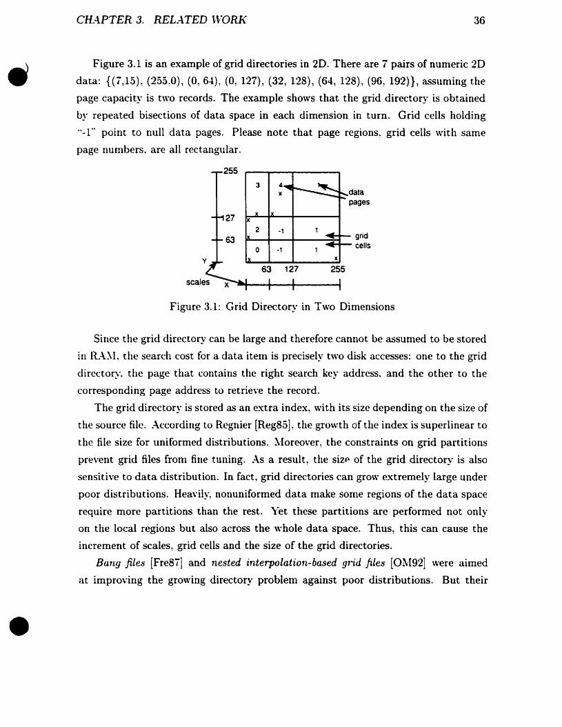
CHAPTER 3. REL.-\TED ~V'ORK 36
•
Figure 3.1 is an example of grid directories in 2D. There are 7 pairs of numeric 2D
data: {(7,15), (255,0), (0, 64), (0, 127), (32, 128), (64, 128), (96, 192)}, assuming the
page capacity is two records. The example shows that the grid directory is obtained
by repeated bisections of data space in each dimension in turn. Grid cells holding
"-1" point to null data pages. Please note that page regions, grid celIs \Vith same
page nunlbers, are aH rectangular.
gridceUs
Figure 3.1: Grid Directory in Two Dimensions
Since the grid directory can he large and therefore cannot be assumed to be stored
in R.-\~L the search cost for a data itenl is precisely two disk accesses: one to the grid
clirectory. the page that cantains the right search key address, and the other to the
carresponding page address to retrieve the record.
The grid directory is stored as an extra index, \Vith its size depending on the size of
the source file. According to Regnier [Reg85], the growth of the index is superlinear to
the file size for uniformed distributions. ~'Ioreover, the constraints on grid partitions
prevent grid files from fine tuning. As a result, the sizp of the grid directory is also
sensitive to data distribution. In faet, grid directories can grow extremely large under
poor distributions. Heavily, nonuniformed data make some regions of the data space
require more partitions than the rest. Yet these partitions are performed not only
on the local regions but also across the whole data space. Thus, this can cause the
increment of scales, grid cells and the size of the grid directories.
Bang files [Fre87] and nested interpolation-based grid files [ON192] \Vere aimed
at improving the growing direetory problem against poor distributions. But their

CHAPTER 3. REL.-\TED UlORK 37
improvements on index sizes are based on tree structured directories, resulting in
logarithmic search cost to the size of a problem, which differs from the direct access
nlethods (0(1)).
l\1ultipaging
~Iultipagingwas invented even before grid files. Like grid files, the kD data space is
partitioned rectilinearly by (k-l)D hyperplane parallel ta aIl a"{es except the one which
it iotersects orthogonally. The partitions inlpose a grid of hyper-rectangles in the kD
space. Every hyper-reetangle can he addressed by k 10 arrays called scales. just as
in grid files. The main design difference is that there is a one-to-one correspondence
between a hyper-rectangle and a data page. [n addition, a scale of a dimension is
obtained based on partitions on the specifie set of data distributed over that field;
each range of values of an attribute field is partitioned ioto m intervals such that
there are approximately the same number of records located on each interval.
ew recordIl
1 3 anIl ~ Il /
x~li
a 2. li
data pages rQl r;I~l.L!.J ~ ~
Page 3 has an overflow record which is stored on page 2.Therefore page 3 has a pointer ta page 2.
(2)
255
(' )
3 .....-~ datapages
32
a 2
scales
Figure 3.2: ~Iultipaging in Two Dimensions
•
Figure 3.2(1) shows an example of a 2 x 2 multipage space, \Vith the same data
as given in the grid file example (7 pairs: {(7,15), (255,0), (0,64), (0, 127), (32, 128),
(6-L 128). (96, 192)}). The numbering of data pages are shown for reference only. It
is in the column-major arder for the 2D array.
If data is poorly distributed~ it is likely ta have overflow records on sorne pages.

CH.-\PTER 3. REL.4TED ~VORK 38
•
•
O\'erfiow records of a page can be stored on a chain of pages starting with the most
enlpty page. or they can be chained onto separate overflow pages. For example!
figure 3.2(2) shows that when record (200!100) is inserted into page 3, it makes the
page overflow. \Vith the firs! collision resolution strateg)'! a pointer on page 3 is used
ta point ta page 2 where the record is actually stored.
In the absence of knowledge of the shape of the data space! it is reasonable to
assunle that it is hypercubic. with a.xes of equal length! n l/k. where n is the number
of total pages. Then scales in kD are of size kn l/k. and can easily be fit in R.-\~l
- there is almast no storage overhead. Thus ideally! multipaging can retrieve any
record for an exact match in exactly one disk access. If there are overflow chains.
more accesses might be needed. Poorly distributed data may cause many overflow
records and long overflow chains. and thus increase the search cast. Distributions of
a diagonal line and a circle in 2D are t\Vo examples of pathological distributions for
multipaging.
One way to reduce the length of overftow chains is to reduce the load factor. the
ratio of accupied space ta available space! i.e.! multipaging allows storage space ta be
traded for access cast.
There are \'ersions of multipaging bath for statie and dynamic data [~I081b.
~I082]. The former uses an algorithm ta analyze the data in O(kn log n) time. and
deternlÎnes the storage utilization and expected number of probes possible for a mul
tipaged file. The latter salves the problem of representing dynamic multidimensional
arrays. and controls either the storage utilization or the expected number of probes.
3.2.2 Logarithmic Access ~Iethods
R-tree Family
R-trees \Vere first proposed by Guttman [Gut84] as a direct extension of B-trees for
spatial data in multidimensians. Like B-trees! R-trees are height-balanced trees. A
leaf node of the R-tree is of forro (oid! R)! where oid is an abject identifier in the
database~ and R is a minimum bounding rectangle (:\'IBR) approximation of the data
abject. R is of the form: (bo• bl ! '''! bk-d, where bi represents the i th coordinate pair

CH.4PTER 3. RELA.TED \VORK 39
L
•
•
of the lower-Ieft and upper-right corners of a kD hyper-rectangle b. An internai Dode
of the R-tree CODsists of (ptrChild, R) pairs, where ptrChild is a pointer ta a child
Dode in the next Dode level. and rectangle R is the ;\,IBR of aU rectangles on the child
Dode.
If .\1 is the maximum Dumber of entries that cao fit in a node, and m $ JI/2
is a pararneter specifying the minimal nurnber of entries in anode, then the R-tree
satisfies the fol1owing conditions:
1. The root Dode has at least t\Vo children unless it is a lear.
2. Every node contains between m and JI entries unless it is the root.
3. .-\11 leaves appear on the same levelt .
4. For every entry in a leaf Dode. oid represents the smallest rectangle that spatially
cantains the kD spatial data abject.
;J. For every entry in a non-Ieaf node, R is the smallest rectangle that spatially
contains ail rectangles in the child node.
E
r r - - ,.....-----,Ile"
A"l ,
....&.....-+-'.... - - - - - 'T 1
1
1
1 1
8 __:Figure 3.3: Rectangles Organized ta Form an R-tree Structure
Figure 3.3 shows the structure of a R-tree and the containment and overlap
ping relationships among its rectangles. The R-tree families have many members,
including packed R-trees [RL85] for statie data, R+ trees [SR87] \Vith guaranteed
disjointness of nodes, R *-trees [BKSS90] \Vith a complex but effective node splitting
tThe first three properties are the same as a B-tree. except m = r~\l/21 for the B-tree.
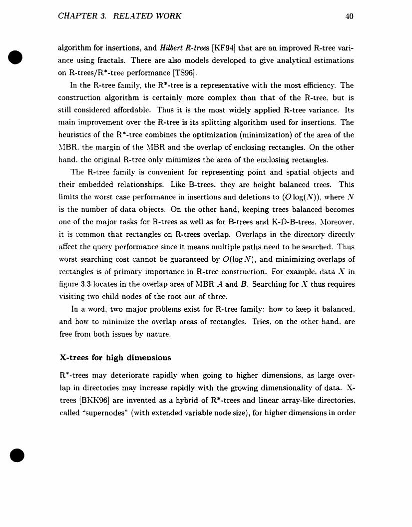
CH.4PTER 3. REL.~TED \~rORK 40
•
•
algorithm for insertions, and Hilbert R-trees [KF94] that are an improved R-tree vari
ance using fractals. There are also models developed to give analytical estimations
on R-trees/R*-tree performance (TS96].
In the R-tree family, the R*-tree is a representative with the most efficiency. The
construction algorithnl is certainly more complex than that of the R-tree, but is
still considered affordable. Thus it is the most widely applied R-tree variance. Its
nutin inlprovement over the R-tree is its splitting algorithm used for insertions. The
heuristics of the R*-tree combines the optimization (minimization) of the area of the
~IBR. the margin of the ~[BR and the overlap of enclosing rectangles. On the other
hand. the original R-tree only minimizes the area of the encIosing rectangles.
The R-tree family is convenient for representing point and spatial abjects and
their enlbedded relationships. Like B-trees, they are height balanced trees. This
linüts the worst case perfornlance in insertions and deletions to (0 10g(lV)), where ~V
is the number of data objects. On the ather hand, keeping trees balanced becomes
one of the major tasks for R-trees as weIl as for B-trees and K-D-B-trees. ~Ioreover.
it is cornman that rectangles on R-trees overlap. Overlaps in the directory directly
affect the query perfornlance since it means multiple paths need to be searched. Thus
worst searching cost cannot be guaranteed by O(log ~V), and minimizing overlaps of
rectangles is of primary importance in R-tree construction. For example, data .\ in
figure 3.3 locates in the overlap area of ~IBR .-l and B. Searching for .\ thus requires
visiting two child nodes of the root out of three.
In a word, two major problems exist for R-tree family: how to keep it balanced,
and ho\\' to minimize the overlap areas of rectangles. Tries, on the other hand, are
free from both issues by nature.
X-trees for high dimensions
R*-trees may deteriorate rapidly when going to higher dimensions, as large over
lap in directories may increase rapidly with the growing dimensionality of data. X
trees (BKK96] are invented as a hybrid of R*-trees and linear array-like directories!
called "supernodes:~ (\Vith extended variable node size), for higher dimensions in order

CH_o\PTER 3. REL.4.TED \VORK
to reduce the overlap problem in R*-trees.
41
f~""""""""" "1
:"0: 4::: -: :~ . . .". . .o. • •
" . .
I:~:l" " ITIJnormal directory node supemode
•
(a) data objects (b) R*-tree (c) X-tree
Figure 3.4: Example of X-tree Structure
Figure 3.4(c) shows a simple example of the X-tree structure for data objects
shown in figure 3.4(a). For comparison, the corresponding R-tree is also given in
figure 3.4(b). It is a 2D example containing 4 data abjects. These abjects have size l~
2. 1 and 3 units respectively. and they are inserted according ta their numeric order.
\Ve assume the maximal overlap allowed in the directory is 1 unit for X-trees, the
maximal directory capacity AI is 3 members, and the minimal capacity m is 2 for
bath the X-tree and the R*-tree. For the R*-tree~ when data abject 4 is inserted
after abject 1. 2 and 3. a split of the root containing the first three abjects has ta be
performed since the capacity of a directory node is 3. The split should partition the
four objects into two groups. each holding t\Vo objects. Note that the overlap area of
~[BR .-\ and B on the root of the resulting R*-tree is 2 units.
If anode splitting using the R*-tree algorithm \Vould make the overlap exceed a
predetermined threshold value~ the X-tree insertion method tries a so called "overlap
minimum-spliC algorithm without considering the balance of the number of members
in each group. If the second try fails due to a minimalload factor requirement on
every node, a supernode is generated instead of a normal node split. The rationale
is to improve the search by replacing part of the expensive hierarchical search (due
to overlaps) by a cheaper linear search within the supernode. In our example, when
inserting object .1. the R*-tree split algorithm is tried first. Since the overlap of .4
CHA.PTER 3. REL..\TED "\TORI< 42
•
•
and B is 2! greater than the threshold value of 1 unit, it then tries the "overlap
minimum-splif' which generates two groups - object 1,2!3 in group one and object
-l in group two. It is indeed an overlap free split. Unfortunately, it does not meet
the minimal node utilization requirement (m = 2), and thus fails the second attempt
for a splitting. As a result, a supernode of capacity 2 x Al = 6 is generated instead.
holding aIl four objects. Figure 3.4(c) shows the resulting X-tree containing only a
supernode. Searching an object in rectangle 2 by the X-tree becomes a linear search
of the supernode in figure 3.4(c) instead of a traversaI of aIl the R*-tree nodes in
3.-l(b).
Obviously! a problem \Vith the X-tree is that in very high dimensions, the con
struction algorithm may fail to generate a hybrid hierarchy structure at aU; instead,
the whole tree deteriorates into one single supernode. As a result, the search becomes
a linear search of the directory. Although this linear search might still be more ef
ficient than tree searches by the R*-tree, it is likely oot the most efficient method
available. In addition. the construction cost of the X-tree is much higher than that
of the R*-tree.
There are many other structures for high dimensional data. Among them are the
T\'-tree (LJF94L the hB-tree [Lom90], the SS-tree (\VJ96] and the SR-tree [KS97a),
etc.
The TV-tree improves the performance of the R*-tree for higher dimeosional data
by employing the reduction of dimensionality and the shift of active dimensions. But a
restriction is that it requires an ordering on dimensions based on importance, and the
dimensionality is reduced by activating only a few of the more important dimensions
for indexing.
hB-trees [Lom90] are based on K-D-B-trees and the idea of '"holey-bricks", bricks
in which subregions have been extracted. The internode search and growth processes
of hB-trees are precisely analogous to the corresponding B-tree processes. The in
tranode processes use k-d trees as the structure within nodes. Node splitting results
in a k-d tree split which produces nodes no longer represented by brick-like regions
in k-space, but rather as holey bricks. hB-trees have been invented to obtain high
storage utilizations of the directory.

CHA.PTER 3. RELA.TED ~\I0Rl( 43
•
•
The SS-tree and SR-tree are t\Vo index structures especially designed for high
dimensional nearest-neighbour queries.
Unlike tries that give data compression, aIl the above index structures require
extra space for directories. The utilization (load factor) of directory pages and data
pages is normally between 1/2 and 2/3.
K-D-B-trees
K-D-B-trees [RobSI] extend B-trees to multidimensional space. The data space is
recursively partitioned into hyper-rectangular subspaces, each of which corresponds
to a page. The k-coordinates of each point in a data page correspond to the k key
attributes of a tuple in a page. It is Ilot specified how subspaces are to be represented
in the index pages. A splitting of bath data and directory pages can be performed on
an arbitrarily chosen point along an arbitrarily chosen partition a.xis. The method in
generai has to cascade a split downwards through every Iower levei of the tree to the
leaves \Vhen a directory page is split. This is a severe drawback, since the insertion
costs and the minimal occupancy of the resulting pages have no guarantees.
:\ Iater attempt by Freeston [Fre95] is also a generalization of B-trees to k dimen
sions. The new BV-tree is designed ta have a guaranteed mininlal page occupancy of
1/3. The trade-off is that it is no longer a height-balanced tree.
3.3 Jaïn Aigorithms
3.3.1 General Review
Joins are one of the fundamental database operations. Since the invention of the
relational data model in the early 1970's [Cod70] , many join processing techniques
have becn proposed and investigated. Basically, there are three classes of join algü
rithms according to implementations: nested-Ioops joins, sort-merge joins and hash
joins. Early database query processing schemes were based on either nested loop
(nested block scans) joins or sort merge joins. Hash based joins \Vere proposed Iater
to improve the join performance. ~Iishra et al. [NIE92] have written an overview of

CHA.PTER 3. REL.-\TED \VORI( 44
•
•
many of the three classes of join algorithms. There had been a long debate on the
issue of the best join schemes (sort merge joins or hash joins) until recent compre
hensive studies showed that there exist dualities between the two (GLS94]. Current
commercial databases support bath of them.
There are man)" ways ta classify join algorithms. They could be grouped by
whether the algorithm uses special indexes such as join indexes (Va187, B~[90], or
by different jain operators. The join operator can be equijoins (including naturai
joinsL and non-equijoins, including band joins (DNS91, LT95], division joins, etc.
Join algorithms that are efficient for one type of join predicates may not be efficient
for another.
~[eanwhile, there has been a lot of effort placed in the development of efficient
join algorithms for parallel and distributed database systems (~[E92, CY"96, HCY97].
Efficient spatial join algorithms have become a new focus for database researchers.
According ta whether indexed structures are used or DoL spatial join algorithms can
be classified as joins based on special data structures, such as R*-tree joins (BKS93,
HJR97] and seeded trees (LR94], and non-index based join algorithms, such as size
separation spatial joins (KS97b], spatial hash joins (LR96], partition based spatial
merge joins [PD96], etc.
:\"evertheless. natural join operations are one of the most critical and fundamentai
operations for efficient query processing. ~Iany such joins algorithms have been pro
posed since the 70s. The relatÏ\'ely recent algorithms among them include Joins by
Fragmentat'ion(.JF) (Sac86], Distributive Join(DJ) [NP91], Stack Oriented Pilter Tech
nique (SOFT) joins (S~I94] and B'Ucket Skip Alerge Join (SSNIJ) algorithms [KR96].
These natural join algorithms apply one or more of the following strategies:
• partitioning (see next section):
• avoiding duplicate page accesses;
• skipping page accesses whene\'er possible:
• using special (extra) indexes.
Overall, there is no single algorithm that is the best in aIl cases; a proper algorithm
should be chosen based on the characteristic of an application. Furthermore, to the

CH.4.PTER 3. RELA.TED \tVORK 45
•
•
best of our knowledge, there has been no work on join algorithms that takes the
advantage of structures that directly organize the data, Le., witbout using extra
indexes, for better join performance, and yet achieving spatial compression at the
same time.
3.3.2 Sorne Representative Join Aigorithlns
\Ve consider joins of large relations that cannot be held in RA~L First, we will review
several join algorithms under the assumption that values of join attributes are unique.
In the last subsection, we will discuss the situation when duplicate join attributes are
present.
3.3.3 Sort-Merge JoÏn (SMJ)
The standard sort-merge join is executed in t\Va steps. In the first step, the t\Vo
relations Rand Sare sorted according ta their join attributes. This can he done
llsing a (8-1 )-way disk merge-sort algorithm [BEi7]. Since the number of passes of
the relation during the sorting is flog(B-l) ~Vl (see Section 1.3 for symbols), the 1/0
cost of the merge-sort is
where ;.VR! ;.Vs is the number of records in Rand S. The second step is the merge
scan, during which both relations are scanned in the order of the join attributes, and
tuples satisfying the join condition are merged to form the output relation. The 1/0
cost of the merge-scan is exactly l'in + ;.Vs if the join attributes in R or S have no
duplicates. Otherwise. the cast may not be linear [BE77, Sac86]. See more discussion
in Subsection 3.3.8.
The sort-merge join algorithm has found to be the best choice if there is no indexes
available on the join attributes, if not much is known about the selectivity, and there
is no basis for chaosing particular algarithms [BE77, Su88, ~IE92].

CHAPTER 3. REL..\TED ~\lORK 46
•
•
3.3.4 Stack Oriented Filter Technique (SOFT)
Among the recent techniques of join operations, partitioningf has been found to not
onlyease parallelization but also improve the overall efficiency. The basic idea is to
partition the input relations Rand S into m disjoint sub-relations Ri and Si, where
Ri and Sj are disjoint if i =1= j, i = L ... ~ m, such that
RMS= L Ri C'<I Sii::::L. •..•m
SOFT. hashed loop joins[DG85], JF and DJ are sorne of the join implernentations
of the technique.
In SOFT. joining sets are repeatedly divided by a ma.ximum of live statistically
independent hash functions until a partition of both joining sets is found to have an
identical join attribute. \Ye will not discuss SOFT further as it uses stacks during the
partitioning process and assumes that data sets can fit in RA~[, while our interest.
as mentioned at the beginning, is in large data sets stored on secondary storage.
3.3.5 Joïn by Fragment (JF)
.-\s a representative partition based hash join algorithrn, .IF applies relatively similar
ideas to SOFT. FirsL it partitions the joining datasets recursively into disjoint subsets
by hash functions. with the use of B blocks of memory buffer. The difference is that
the partition continues until aoy subset from the smaller relation can fit into a memory
buffer of size B - 1. In this \Vay the .IF algorithm partitions the data sets without
sorting them. Then it performs the join by a merge-scan of subset pairs.
Figure 3.5(a) gives relations Rand S. Figure 3.5(b) shows the merge-scan phase
by JF. assuming the block capacity is -l data items. In the figure, sets Rand S have
been partitioned iota fragments bya hash function before the merge-scan phase. The
hash function used during the partition is k mod 2, Le.. the first fragments for Rand
S hold odd \·alues, and the second fragments hoId even values.
tIn the literature. it is inaccurately referred to as ·~divide-and-conquern. Strictly speaking,divide-and-conquer is a strateg)" for reducing asymptotic complexity, such as sort from O(N2) taO(N log N) .

CH.-\PTER 3. REL.4TED nlORK 47
118.2.~.161 C><J 1 8.2.12.1 O.~.6.1~
[c' Distributive Join:
R Ssubsct \2. 3.~. 5 1 [><J 1 3.S.I.2A 1
R: 13.18.5. 2.~. 17. 16.3• (a) Joining SelS:
(b) Join by FragmenlS:R
1 13.5.17.31
S
C><l 111.3.5.9.1.15.7.13
S: 11. 3. 5.8.9. 1.2. 15. 12. 10.~. 7. 6. I~. 13
partial join 1 result
-1 13.5.3
- 1- - ~ 12.-'
partla Jom-
rcsultpartial join 1 2.3A.5-
subsct p.16.L7.181 [><J 111.8.9.15.12.1O.7.6.1~.13 I---~_~ IL....I_3__-J
partial join 2
td) Buckct Skip Merge Join:
Join auributc values
13
resuhRC><J S
High
High
Law
buckcttable low value high value ptr
forS 1 ~
2 5 8
3 9 12
~ 13 15
Low
low value high value ptr
2 5
2 13 18
High
High
Low
Low
buckcttablefor R
High - Buckct portions matwere skipped
Law Indic3ting pointer
~ traversai during
High mcjoin
Law
1,...-- ....J
,1
1,
•Figure 3.5: Three Join ~\'[ethods for Data Set Rand S
CH.-\PTER 3. REL.4TED n/'ORK 48
•
•
The 1/0 cast of JF contains t\Vo parts. the partitioning cost and the merge-scan
cast. \Vith the use of B blacks in memor'y~ JF applies the hash function (k mod (8
1)) ta partition Rand S into B - 1 sub-groups. Subsequently, it divides the subsets
recursively until one of the resulting subset ~ and Si has no more than B - 1 blacks.
In case of unifornl distributions. if the number of partitions is kR for relation R, then
.VRI(B - l)k R ~ B - 1. Therefore
Each application of the hash partition on R has an lia cast of
.-\S a result. the cost of completely partitioning R or S is
where i = R or S. :\"ote that this is lower than the sorting cost by S~IJ. In case of
no duplicate join attribute values in R or S. the merge-scan phase is just ~VR + ~Vs
(same a.s S~['J) and the total cast of the JF is therefore
Like other hash partition join techniques. the JF algorithm is particularly suitable
when indexes for joining attributes do not exist and the data is unsorted.
3.3.6 Distributive J oin (DJ)
.\lthough sharing the same "divide and conquer:' idea as JF l the approach by DJ is
different. DJ belongs ta the ··sort-merge·' category. But it improves the standard
sort-merge algorithm by avoiding completely sorting bath input data sets on the join
attributes. Instead, it only sorts the one with the smaller amount of data completely
and partitions it into subrelations. The size of the subrelation is less than that of
the available R-\~I buffer. The boundary values of these subrelations are stored in a

CH.-\PTER 3. REL.-\TED \-VORI( 49
•
•
table calied the distributive table. Theo the large relation is partitioned and partially
sorted using the distributive table. The DJ algorithm, therefore saves part of the
sorting cost. There are three steps in the algorithm:
1. completely sort the smaller data set into ordered subsets (R1l R2 , ••• , Rm) \Vith
each subset size no more than B -l, and produce a distributive table containing
baundary values of the joïn attributes of the subsets;
2. distribute the larger data set inta subsets using the values in the distributive
table as the boundaries of its subrelations using a partial distributive sort;
3. perform the join bet\veen the sorted and the distributed sets.
Figure 3.5(c) shows the merge-join phase of sets Rand 5 given in figure 3.5(a).
Before the nlerge-join. set R has been sorted into t\Vo sets, while set 5 has only been
sorted partially.
The cost of DJ consists three parts: the cost of complete sorting of the smaller
relation R, (2~VR rloga_1 ~VR1), the cost of distributing the larger relation S into
r~VR/(B - 1)1 subsets, and the cost of merge-join bet\Veen ~ (sorted set) and Si
(distributed setL where i = L ... , m. The last part is (JVR + 1VS ) in the absence of
duplicate joiIl values. Csing a B - l way distribution algorithm on secondary stor
age. the number of passes to distribute S into m subrelatioos is [098 _ 1r~VR/(B - 1)1,
which is strictly smaller than the number of passes to sort S completely by S~vIJ in
most cases [~P91]. Therefore at least one pass of the large relation can be saved in
conlparison to 5:\IJ.
3.3.7 Bucket Skip Merge JoÏn (BSMJ)
The 8ucket 5kip :\lerge Join (85:\IJ) improves 5:\IJ by creating and maintaining sorne
extra storage, bucket tables 00 secondary storage, to hold upper and lower values of
join attributes for each data bucket (page) as \Vell as pointers to corresponding data
buckets. The bucket table entries are first accessed during the join processing in order
to avoid data bucket fetches and attribute comparisons in R..-\NI whenever possible.

CHA.PTER 3. RELA.TED \l"ORK 50
•
•
BS~'IJ has its great advantage over aH hash joins including JF and DJ in the situation
that the input sets have been sorted and indexed.
Figure 3.5(d) shows bucket tables, data buckets, file pointer movements of the
bucket skip merge join on Rand S in figure 3.5(a) and the result of the join. The
shaded area is the bucket portion that has been skipped during the join.
BS~[J focuses on sorted relations. By maintaining extra storage for bucket tables,
the cost of merge-join can be less than one pass because of the skip factor, when there
is no duplicate values.
3.3.8 Duplicate join-attribute values
In the presence of duplicate values, the cost of aIl above join algorithms may increase.
\Vhen DJ algorithms are applied to duplicate values, the cost to distribute the
larger relation increases in order to meet the restriction that aU tuples having the
same \'alue of join attributes nIust belong to the sanIe subrelation. This suggests
there may be nI0re subrelations in the presence of duplications. But it has been
prO\'en that with duplicates, the extra cost of distributing the larger relation can be
no nl0re than one pass than without duplicates (NP91].
The cost of both partitioning and/or sorting is independent of data distribution
and duplication for S~IJ, JF and BS~I.J algorithms. It is only the final join phase
that is affected by the duplicate values. If sorne of the duplicate join values exceed
the capacity of the available buffer in R:\~L aU S;\;IJ, DJ, JF and BS~IJ algorithms
are forced to apply nested block scans. and the cost of merging can become quadratic.
3.4 Summary
The chapter gives a literature review on ID to multi-dimensional data structures,
direct access method to tree structures. as weil as a review on join algorithms. In
conclusion, there does not exist a single approach as a solution for aIl the problems
posed by one dimensional to multidimensional data. low to high selectivity, special
to structured data, efficient in both space and time and distribution independence.

•Chapter 4
Tidy Functions
4.1 Piece-wise Linear Tidy Functions
Let us look at the tidy function definition fronl section 3.1.2:
t =fn D(x)l (ot1)
•
where x is a key and n is the number of pages on secondary storage. If t has to be
stored in its full resolution~ it nlay exceed the RAJ\I capacity for large files. Indeed~
it is valuable to make the assumption that RA~I capacity is 0(1) while file size is
O( n). Tidy functions stored on secondary storage will not only increase the storage
cost but also the retrieval time. A solution for this is a piece-wise linear interpolation
of nD(x). which results in a so called piece-w-ise linear tidy function.
Assume that the number of linear pieces~ p~ is given, the tidy function can be
represented by 2p numbers with 2(p - 1) pairs of x and nD(x), the range of keys and
the total number of pages n. This tidy function is certainly a bigger structure and
more complex to calculate than a simple hash function, such as x mod n. But it is
small and quick compared to secondal}' storage which it is addressing. Here, p « n
is bounded by R--\~I capacity, and has a data distribution dependency as weil.
\Ve assume that the file is loaded onto pages in key order just like a sequential
file. The load factor can be as high as one~ i.e.~ our tidy function is indeed an order
preserving minimal hashing fUfiction. But it need not to be one; there can be empty
51

CH.-\PTER 4. TID1- FU1VCTI01VS 52
•
•
space in our file. In this case~ we simply have a different distribution function to
approximate. and the tidy function is an order preserving hashing.
Overftows
page boundaries
4
3
2
1
xFigure .t.l: .-\ Distribution Function and a I-piece Line Tidy Function
Figure .1. l shows a distribution function nD(x) and a one-piece linear approxima
tion tidy fUIlction L(x). Three horizontal lines are drawn at page boundaries from
nD(x) to L(x). \Ve shaH show that these lines represent the overflow keys that the
tidy function L(x) gives the wrong page address. For example, key a maps to page
3 according to tidy function nD(x). but according to the approximate line L(xL it
should be on page .t. .-\S a matter of facto L(x) maps any key on the three horizontal
lines between nD(x) and L(x) at page boundary L 2 and 3 to a wrong page address.
Thus these horizontal lines at page boundaries represents aU possible records which
will cause the search to make at least one extra probe. The SUffi of the length of
these lines gives the total number of overflowing records. For continuous key space
this hoIds strictly, but we still get the right proportion if the key space is discrete.
The ahove discussion counts both successful and unsuccessful searches. ~Iore often,
successful searches are more useful and one should only apply records present on those

CH.-\PTER 4. TIDY FUNCTI01VS 53
• horizontallines between the tidy function and the linear pieces at page boundaries.
Now we show that the area between nD(x) and L(x) gives approximately the total
number of overflows. This is because the horizontal Hnes drawn at page boundaries
are equally spaced vertically~ by a distance of a page, h. Each section of the area
between L(x) and nD(x) is approximately a parallelograrn of height h and length bil
the length of the horizontal line. \Ve have
Clearly, the area is proportional to the total length of horizontal Hnes drawn at page
boundaries which represent the total overflow. In other words, the area between the
tidy function nD(x) and the approximation linear pieces L(x) gives the total nurnber
of extra probes.
\Vhen overftows oceur, different relative positions of L(x) and nD(x) give different
extra probings. If L(x) is above nD(xL the linear probing is downwards frorn the
target page of the tidy function ta the page it truly presents. The linear probing is
upwards when L(x) is below nD(x) . .-\ny page that contains an intersection of nD(x)
with L(x). with nD(x) starting abave and crossing clawnwards under L(x), will have
no overftaws. On the other hand. any page with an opposite intersection will overftow
in both directions and thus needs both downwards and upwards linear probings.
Obviously. the goal of the piece-wise linear tidy function approximation is to find
a set of p points on nD(x) with minimal overftows. i.e., the minimal surn of the length
of horizontal lines. or the Ininirnal area between nD(x) and L(x).
Analytical Example
\Ve start to minimize the overftow with a simple analytical exarnple D(x) = x 2 , \Vith
x E [0,1), by two linear pieces. Assume that the t\Vo pieces meet at (z, Z2). Then
L(x) contains t\Va pieces: L1(x) = zx and L2 (x) = (1 + z)x - z. The area between
the t\Va curves are
•fo
= 2 fI,) 1 2 1(zx - x )dx + ((1 + .:)x - z - x~)dx = - (z - z + -)
a = 2 3(4.2)

•CHA.PTER 4. TID1· FUNCTIONS
After minimizing the above~ we get
dl,} 1 1- - (z- - :; + -) = z - - = 0 => z = 1/2dz 2 3 2
54
•
50 the optimal approximation by t\Vo linear pieces is ta partition the range of search
keys at the middle. Similarly. we can minimize the overflow \Vith three pieces of L(x)
for D(x) = x 2 at points (Zl~ZI2) and (':2,Z22
). The calculation gÏves ZI = t and
4.2 Heuristic Construction Aigorithms with Min
imal Overflow
In practice. distribution functions are not analytical. For distributions of interest, we
find that we can turn ta dynamic programming to get the optimal partitions with
minimal o\·erflow.
Let men, p) denote the minimal overflow cost if we use p Iinear pieces to approx
imate the distribution function nD(x), and d( i, j) be the overflo\\" cost of the line
piece if we connect point i to j with a straight lîne. Then men, p) can be recursively
defined as fo11ows:
m(n,p) = m.znp<i<r.{m(i.p - 1) + dei, n)}
where Tl is the number of pages, 0 < i < n and p is the number of linear pieces. A
brute-force method to calculate men, p) costs O(nP ). Dynamic programming solves it
by calculating and storing e\'ery possible value of m in a n x p table~ and d in a n x n
table, and therefore avoids recomputation of every entry in these tables. A bottorn-up
calculation of the table elements is used, from m(l, 1),m(2, 1), m(2, 2), m(3, 1), m(3, 2),
... ~ m(i, jL ..., to m( n, p). It turns out that the cost of this dynamic programming is
O(pn2 ). This is tao many disk accesses to be acceptable. Instead, we propose a less
expensive heuristic construction algorithnl which cao also make the optimal use of p
linear pieces br applying them to the Hne segments \Vith ma.ximal overflow.

CH!\PTER 4. TIDY FUNCTI01VS 55
• \Vith the new rnethod, systematically, we look for straight segments of the distri
bution, and to fit the longest and straightest of these segments using as nlany of the
p pieces as we can; i.e., we look for sections with zero curvature.
\Ve do this by bounding nD(x) with a sequence of parallelograms, iteratively
splitting the most expensive one until there are p parallelograms. The first steps are
shown in Figure ~.2.
(a) distribution function nD(x) (b) connecting from end to endwith a straight Hne. L(x)
(d) forming two linear piecesLI and L2
,,,,,,,,,1 ,
~'
,1
" 1, 1
, 1
" 1, 1,,,,
break point ,,'~ ,,'-'-~
(c) forming a bounding parallelogramwith breakpoint at the maximum verticaldistance from nD(x) to L(x)
Figure ~.2: Forming a Bounding Parallelogram in Tidy Function Construction
•
\Ye start by connecting nD(x) from end to end with a straight Une (Figure 4.2 (b) ).
Then we look for the point on nD(x) which has the ma.ximal vertical distance from
the Hne (Figure ~.2(c)); this maximum vertical distance corresponds to the longest
o\"erfiow chain from the page which the straight Hne indicates the record at that point
is on, to the page it is really 00, according to nD(x). \Ve cali the point ;~breakpoint",

CHAPTER 4. TIDY FUIVCTIONS 56
•
•
for it is chosen as the endpoint of two new straight Hnes (Figure 4.2(d)). Consiclering
each of these lines as an approximate tidy function, we calculate the overflow cast for
each. The segment \Vith the larger cost is the next candidate for splitting. For the
candidate segment, we repeat step (c) and (d) in Figure 4.2. Thus, we again find the
point of nD(x) in this segment that is the maximum vertical distance from the line.
and make it the endpoint of t\Vo new straight Hnes. As an example, these first few
steps are shawn in Figure 4.3.
.- 1.- 1.-,
.-- - -_._------"---_.,. ..~ - ,-'-~ ---,
......
pages
kevs
Figure ·t3: Finding p Segments of Zero Curvature: First Steps
In the end. we have a fit to the original distribution, such as shown in Figure -lA.
The example sho\vs a fit of 10 pieces to an original data distribution lOOD(~') given
in Figure 4.3. The numbers from 1 to 9 on the curve correspond to the iteration at
\Vhich the point is selected as the ;'breakpoinf'.
The parallelograms that we show in the figures serve to indicate the furthest
vertical point of the distributions. Clearly, the skinnier the parallelogranl is. the
more nearly the part of the distribution function it bounds has zero curvature. and
the longer they are. the more useful a linear approximation is to the segment. The
heuristic construction algorithm is outlined in Figure 4.5, where Q serves as a queue

CH:\PTER 4. TIDY FUjVCTI01VS 57
,-5
./
.0-8 __ -
100 -===-=--==::-:::::.-=c:-=--~-----~~-----.. ~.
95 . -~ -- original CUNe with 99 pages -4" --90 . -.- t 0 approximating line segments85 •----~----~----.
80 .75 .70 .65 .60 .55 .50 .45 •40 .35 •30 .25 .20 .15 .10 .5 .o .-,- -_., .- ---~.- -_.~ ,-- - .... - .0 ~~._.~ ~---~.
2.09+083.0e+084.0e.085.0e.086.0e+087.09+088.0e+089.0e+081.09.091.1 e.09
•
values of keys
Figure -tA: :\ Tidy Function \Vith 10 Linear Pieces
of candidates for splitting, ordered by decreasing overflow cost.
~ote that building our tidy function requires an initial pass of the whole file to load
the data and to extract only those keys marking the boundary of pages. Thereafter.
we work with the set of n keys, which we caU a pagekey file.
The \Vorst case cost of the above construction algorithm happens when the ith
breakpoint has to be found among n - i + 1 page keys, and the search has to look
over n - i + 1 page keys. It happens when the p - 1 breakpoints are where the first
(or last) p - 1 page keys are located. Therefore~ the total cost is
p-l
~(n - i + 1) = (p - 1)(n + 1) - O.5p(p - 1) = O(pn)i=l
•
This corresponds to about p passes of the page keys.
The lowest construction cost happens when the data distribution is uniform and
the breakpoint is always the kt.h point of 2k points in any linear piece. Thus finding
the i th breakpoint means checking through ni Llog2(i + l)J page keys in the range.
Therefore the best construction cost isp-l
2: ni L10g2 (-i + 1)J~ n log2 P = 0 (n log2 p)i=l

CH.APTER 4. TIDY FUj\jCTIONS 58
• typedef struct {POINT -staPoint,float overflow;
} Segment;
/- Definition of a Segment -/-endPoint, -brkPoint; /- POINT is a pair:(k, nD(k»-/
typedef struct {Segment -set;int num_elements;
} LineSegmentSet;
/- Definition of a Segment Set */
•
/* num: is the number of line segment pieces- pO, pl: two end points of the distribution function- Q: a queue of candidates for splitting, ordered by decreasing overflow cost./
void tidyConstruction( int num, POINT -pO, Point -pl, LineSegmentSet Q){
Q= {};aSegment= processOneSegment(pO, pl);insertNewElement(Q, aSegment);for ( i= 0; i< num-l; i++) {
aSegment = removeFirstElement(Q); /- take lst member of Q for prccessing-/segmentl= processOneSegment(aSegment.staPoint, aSegment.brkPoint);segment2= processOneSegment(aSegment.brkPoint, aSegment.endPoint);insertNewElement(Q, segmentl); /- insert a member ta Q such tbat the */insertNewElement(Q, segment2); /* overflow cost is in decreasing order */
}}
Segment *processOneSegment(POINT -pO, POINT -pl)/. find the breakpoint and calculate the overflow cost of the segment-/{
Segment -aSegment = new Segment(pO, pl);maxYDist = 0;totalYDist = 0;
for POINT -p= pO to pl {curYDist = verticalDistance(p, Line(pO, pl»;totalYDist = totalYDist + curYDist;if (curYDist > maxYDist) {
brkPoint = p; /* brkPoint is the one with max distance to nO(x) -/maxYDist = curYDist;
}}
aSegment->brkPoint= brkPointiaSegment->totalOverflow= totalYDisti/* overflow is proportional to the sum of vertical distance to nD(x) -/return aSegmenti
}
Figure 4.5: Tidy Function Construction Algorithm

CH.4PTER 4. TID),P FUNCTI01VS 59
•
•
This amounts to about log2 p passes of the page keys. For example~ if p = 25~ OOO~
the least tidy function construction cost is about 15 passes of the page keys.
4.3 Search Algorithms
Searching the data using the tidy function consists of two steps. First. calculate the
page address where \'le expect to find the data using the tidy function stored in RA~C
as we would use a hash function. \Ve caH this page address the home page. Second~
like "collision resolution'~ in hashing~ search the file for the page that really contains
the data. The second step is similar to linear probing in hashing. The difference~
however. is that the probing can be in either direction: either downwards or upwards
from the home page as discussed in section 4.1. If the linear approxÎInate line is above
nD(xL i.e.. the data on the home page have larger value than what we are searching
for. the search will continue downwards. If it is be/ow, the actual data will be above
the home page, and the Iookup will be upwards.
In either case, if the data being hunted is not present in the file (unsuccessful
search). the search must proceed in the appropriate direction(s) until the data values
are above and/or below the one that we are seeking and a failure is discovered.
Our experiments show that in a large number of situations, aH data that is ex
pected to lie in a given home page may in fact be found in a range of pages considerably
above or below the home page for a small number of linear pieces, p~ and irregular
distributions. The above search algorithm can be improved by eliminating the linear
probing through the pages containing no data which are searched for by storing a
pointer on each page pointing ta the nearest page that actually holds rele\'ant data.
\Vhile the o\'erhead is negligible, our experiments show an arder of magnitude search
ing performance improvement for very large files as a result of storing these pointers.
Furthermore. sometirnes even the range of pages holding the actual data maybe
large, and a linear search through the pages after following the pointer is still quite
expensÏ\·e. \Ve can impro\'e the search performance further if a second pointer on
each page. pointing to the furthest in the range~ is used. \Vith the two pointers on

CH.4.PTER 4. TIDl~ FU1VCTIONS 60
each page, we can do a binary search between these two pointers.
D(x)
L(a)
-1D(L (L!--(atn
•
Figure -1.6: Searching and "Collision Resolution" for Tidy Function
Figure .1.6 shows the idea of these pointers by an example. It shows a key a.
mapped by the linear approximation ta page L(a). The bottom of the page is denoted
lL(a)J, and the top is fL(a)l. Data a is actually stored on page nD(a), in a 5-page
range starting sixteen pages above the home page L(a). The bottom page of the
range is page nD(L-l(L(a)J)). and the top of the range is page nD(L-l(f(a)l)). The
two pointers in the home page ta the bottom and top pages are shawn in the figure.
It is clear from the example that steep portions of nD(x) are responsible for large
ranges, and thus large overftows. This happens where the search keys are clustered
closely together and there are not enough linear pieces to closely approximate these
clusters.
•

CHAP TER 4. TIDYFUNCTIO~ 61
• 4.4 Experimental Results
•
Our experiments were conducted on two sets of data. The first set \Vas generated in
the following way to produce cumulative distributions similar ta what are shown in
Figures 4.3 and 4.4. Tl random nurnbers were generated in 9 groups. Each group is
based on a random (0 - 215 ) multiple of 215 , and contains a random number of ele
ments, each of which is generated randomly by mod 227 . After sorting, these numbers
produce values of keys located at the top of each of n pages, and give a cumulative
distribution to work with. Each of these cumulative distributions has 9 major steps,
\Vith nlÎnor fluctuations. However, when 9 gets larger than several hundred, and
n >~ 104 , the big steps tend to disappear and the resulting distribution becomes too
easy to approximate well. So we modify the method by inserting additional random
elernents within the steps in order to increase the vertical scale of the distributions 1
such as those shown in Figures 4.3 and 4.4. By doing 50, we increase the numbers of
extra probes in searching.
The second set of data \Vere real phone data from ProCD, a business phone
book [Pr096]. which contains more than 15 nlillion American business phone num
bers. It \Vas used to verify the results we obtained from synthetic data. \Ve choose
the phone data because the cumulative distribution has big vertical steps, which
challenges our tidy functions.
\Ve will compare our experimental results with Fox's order-preserving minimal
perfect hash method. the closest competitor, in construction time, storage consump
tian. and search time.
4.4.1 Construction
After the initial pass of the whole file to extract the pagekey file of size n, the cost
of finding p linear pieces to approximate nD(x) using our method depends on p.
Figure 4.7 shows the number of passes we must make of the pagekey file in order ta
construct p linear pieces. Since the data describing these p pieces must be contained in
R:\~L we may build up to only 50 many pieces. In Figure 4.i, we stop at p = 25,000,

•CHAPTER 4. TID1
P
FUNCTI01VS
and for these many pieces, the cost is 17.5 passes of the pagekey file .
Number of Passes of Pagekey File to Build p Linear Pieces18ïT"""----"""T"""----"""T"""----......,......-----r-------r-l
16
14
12II)
alII)
~10Q,
'0
~E~
c:
4
2
0L....l--------l......-------l......------I....- --I.... ......I....J
62
a 0.5 1 1.5 2p: number of approximate line segments
2.5
x la"
•
Figure -1. 7: ~umber of Passes of Pagekey File to Build p Linear Pieces
To compare this construction with Fox's method, we make a conservative assump
tion that each page on1y hoIds 10 records, Le., lVln = 10. This is a minimal nunlber.
\Ve also assume that these records consist of nothing but keys. So 17.5 passes of
the pagekey file need the same amount of 1/0 as 1.75 passes of the whole file. This
is much less expensive compared with 6.8 passes for the first cheap stage of Fox's
construction method. \Ve have easily won by an order of magnitude as compared to
Fox in thp aboye estinlate.
\Ve can do another conlparison on construction time from a later paper by Fox et
al.(FHCD92) on minimal perfect hash functions which are not order-preserving. The
construction cost here is lower than the order-preserving hash function by inspecting
the two algorithms. In their paper, they constructed 3.9 million keys into a hash
CHA.PTER 4. TIDY FUNCTIOiVS 63
•
•
function in 33000 seconds on their fastest machine. If we suppose, reasonably, these
keys and their associated records are stored on 400,000 pages, and that each key
consumes 10 bytes, the pagekey file would he 4~'IB in size. \\Te now estimate how
nluch it would take to construct the tidy function on a slow disk with 2J.lsecond
transfer time per byte. One pass of the file would cost about 8 seconds, and 1ï.5
passes would cost 140 seconds. On a shared disk, we would have to access each block
separately. Suppose an average disk seek time and rotation time is 20ms, and a
block size for the pagekey file is 1KB, then 4~IB page keys would he on 4000 blocks
with loading each black costing 20ms+ 1000 x2J.ls = 22ms or 88 seconds per pass.
This translates to 1540 seconds for 1ï.5 passes, or 21 times faster than that of Fox's
method.
Br both comparisons. our tidy function construction method is more than one
order of magnitude faster than that of Fox et al. ).;[oreover, our method is truly
linear. and not almost linear as for the other authors.
4.4.2 Storage
Our method is a minimal perfect hashing, requiring no empty locations in the data
file. The load factor. a, the ratio of occupied space to available space, is l.
The storage overhead of our method is negligible. It stores only a p-piece set of
linear approximations which by definition can fit into R.-\~I, and two pointers per
data page used to set up the binaI}' search for overflows.
Although Fox et al. cIaim a minimal perfect hash function (Q = 1), their method
nlust store an auxiliary table of size 1.261V pointers, or 1.26 pointers per record.
4.4.3 Searching
Figure 4.8 shows our experimental results on searching with the synthetic randomly
generated cumulative distributions and 15 million American business phone numbers
(the crosses on the figure). The cast of searching is a function of file size and p, the
number of approximating linear pieces. \Ve have measured up to 107 pages which may
correspond to at least a 10 GB file. \Vith this size, our expected number of probes

CH.-tPTER 4. TIDY· FUNCTIOl\jS 64
• 7
6
2
Access Cost versus Number of Data Pages
- 1 piece and 25k pieces
- .. 100 pieces
1000 pieces
10000 pieces
x 15M phone data
....
x
x
x
. ~ ....
x
•
O'--~~~........Io..._~-~~----o..·_~..........1--_........--........L_-~..............J1i 1~ 1~ 1~ 1~ 1~
Number of Data Pages
Figure ..1.8: .-\verage Probes per Search versus File Size
ta search the file~ \Vith 25~000 linear pieces~ just gets up ta 3. This is still better than
the 3.25 of Fox et al. Since Fox~s search cast is independent of file size, they would
eventually inlprove our result for large file size. However ~ ta construct a file of lOi
pages. or 108 keys~ by their method would require at least 106 seconds~ or two weeks.
In Figure ·t.8. we also give the search cast tested on the 15 million phone data.
The result matches with what we get from our synthetic data.
It is clear froln Figure ·t.8 that for file sizes massively larger than the allowed
number of linear pieces~ the logarithmic behavior of the binary search takes over from
the direct access behavior of the tidy function. This leads to the natural question
of whether the B-tree should in fact he used. It is indeed true that the search cost
by B-tree can be competitive to tidy functions when the first two levels are stored
in R:\~L However~ the construction cost of B-tree is O(n log n) while our method is
much cheaper - it is O(n) .

CHA.PTER 4. TIDY FUNCTIOltlS 65
• 4.5 Summary
•
In this chapter. we have introduced a class of order-preserving key-to-address trans
formation funetions (tidy funetions) that ean be constructed in linear time and are
significantly faster than the time for the closest competition. Our method requires
no storage o\'erhead while the earlier methods need linear index space on disks. Our
nlethod is simple in conception and the algorithms are straightforward to implement.

•
•
Chapter 5
Tries for One Dimensional Queries
.-\ Inajor weakness of the linear heuristic tidy function we proposed in the last chapter
is that it is intended for static datasets. In this chapter, we propose tries as an al
ternative structure to order-preserving key-to-address transformation funetions. The
gain fronl this is three-fold: dynamic, conlpactness and speed.
5.1 Tries as Tidy Fonctions
.-\ ID trie on the search keys can be interpreted as if it is an order-preserving key-to
address transformation function, even though the former is not direct access method
as the latter. The remaining fields of a data record are stored either on a trie leaf,
or a separate file pointed to by a pointer on the leaf node. The method exploits
the variable-resolution capacity of tries, their order-preserving properties. and profits
from substantial compression achieved using indexed keys.
Construction of the trie consists of two steps: a) convert keys to their binary
representations, and since these keys are in order, so are the binary representations of
these keys. b) perform a batched process of merging trie norles to construct DyOrTries,
similar to OrTrie construction proposed by Shang (Sha94]. Trie paging can he done
during the process by creating a trie page and writing it ta the disk whenever trie
nodes in the page layer exceeds a given page capacity. The construction algorithm
reads the ordered keys once and writes the trie once. Thus. the cost is Hnear to the
66

number of keys and file size.
Using the insertion and deletion algorithms of the DyOrTrie structure proposed
in section 2.6, our trie is capable of inserting and deleting keys at a cost of O(log lV)
page accesses~ where ~V is the number of keys. ~evertheless, the Hnear construction
algorithm is much cheaper than building the trie by dynamic insertions.
To search a data iterrl with a given key, first, we convert the key to its binary
representation, and then look for it on the trie starting at the root. At any trie node,
if the current bit of the binary key is '·0", the search goes on to the left branch, and
to the right brandl if ··r'. \Vhenever a lear node is reached, a record \Vith the given
key is found by following the pointer to the remaining data attributes in the file.
Therefore, the cost of successful searching is h page accesses. where h is the height
of the trie. assuming the root page of the trie can be stored in R.A~vl. :\ search is
unsuccessful if it has to stop at an internai node of the trie at page leveli. The cost
in this case is siroply i-1 disk accesses.
•CHA.PTER 5. TRIES FOR ONE DIAfENSIO:.V.<\L QUERIES 67
•
5.2 Experimental Comparisans with Tidy Func
tians
In order to compare \Vith tidy functions. we use the same two groups of data. as in
the last chapter (unless mentioned otherwise): one is the synthetic nonuniform data,
and the other 15 million American business phone numbers.
5.2.1 Storage
The trie compresses data and can achieve a significant compression rate due ta the
overlap of paths near the root. As the file gets larger, this compression effect becomes
more pronounced. For files consisting of uniformly distributed keys only. figure 5.1
shows that the data compression increases to over 90% as the file gets large. Obviously,
this is superior to the tidy function which needs a small mount of space overhead ta
store information about the p linear segments, and two pointers per page used to set

•CHAPTER 5. TRIES FOR ONE DIAIENSIOlV.4.L QUERIES
up the binary search.
compression ratio vs. 'records
~~-.-- me melhCXl• me methOd ( mil) data)
~~-~._-~~---
68
•
.--.---... - ........ --. -
~ .
1~ 1~ 1~ 1~number of records
Figure 5.1: Trie Compression vs. File Size
5.2.2 Searching
•
Figure 5.2 shows the cost of searching by trie method on nonuniform data sets. This
is compared \Vith the tidy functions of 25.000 linear segments given in figure -1.8 •.
The trie page capacity is fixed at -1096 bytes. This measure also assumes that the
first t\Vo trie page levels are stored in R.-\~1. This is based on the assumption that the
RA~I buffer size can store the information of 25,000 linear segnlents. From the figure,
we sec that for large files (lOi to 108 records), the trie method gives 2 page aceesses,
which is superior to the performance of tidy functions. For small files, the trie is at
least as good as the tidy function method ,vith 25,000 linear segments. \Vhen the file
is small enough and the trie is stored in RAl\L one access to the data page is the only
cost of searching, this happens when the number of records does not exceed 105•
The figure also shows the results from the 15 million entries from phone book
data. It verifies and matches with the results obtained from the synthetic data sets.
• Here file size is given in number of records instead of number of pages. \Ve assume that a pageholds 10 records.

.
•CHA.PTER 5. TRIES FOR ONE DI~"IE~VSI01'iA.LQUERlES
Search Cost versus Number of Data Records
tidy function:synthetic data
3.5 x tidy function: phone data
- trie:synthetic data
3 -- 0 lrie:phone data
~li: 2.5-; x
;' ; ----~
~ 0 •~
;/
;/
/;
_._ J
o
0.5--
Ol--_~-_.l..-_--_..J....-_--_.....,I.-__--.... ...J.... ......J
103 10· 105 106 107
108
Number of Data Records
69
•
Figure 5.2: Average ~umber of Probes per Search \·s. ~umber of Data Records
CH.-\PTER 5. TRIES FOR ONE Dll\IE1VSI01VA.L QUERIES 70
• 5.3 Summary
•
In this chapter~ we have applied the 10 trie method as an alternative ta the order
preserving key-to-address transformation function. The I-d-trie achieves compatible
searching performance to that of the tidy function. The gain is the storage compres
sion the trie achieves~ as weIl as its capability of dynamic insertions and deletions at
a cost of no more than O(1og ~V) page accesses per key.
:\ B-tree \Vith a fanout of 100 and its first two levels stored in RA~I is competitive
in its search cost. \Ve assume that the page capacity is 4096 bytes and a page hoIds
100 records on average. For example, \Vith 108 keys, a B-tree file has four levels and
a total of approximately 106 pages (one root page on the first level, 102 pages on the
second, 104 pages on the third, and 106 pages on the fourth (leaf) level). The cost for
searching a record is t\Vo accesses. which is quite compatible \Vith the trie method.
However, in terms of space cost, there is no \Vay that it can be deemed conlpatible
with the storage compression of the trie structure.

•Chapter 6
Tries for M ultidimensional Queries
In this chapter, we shaH extend tries for nlultidimensional queries~ including exact
match and orthogonal range queries.
\Ve shaH compare our method with that of existing representative multidimen
sional methods. These include direct access methods such as multipaging and grid
files. as well as weH-applied multidimensional logarithmic nlethods such as R*-trees
and their variances X-trees for high dimensional data.
6.1 Variable Resolution Queries
2 3 4 5 6 7
01 10.011 lllE1E:!r--l
10 i'
011 1 : : ioo! Iii 1
- - - - - - - -.... 00 01 10 11
01
1.-J----~mo 1 6;....1~-4---I-~--J--II--!-----1
1
51r--+--+-_4!~I--r--
3 I--~+--+---+--+---+----+-~
-------------------. 21--~~+__~~_+___~I~'
:i:====: '---':--l-tJj~;o 1
x
Figure 6.1: Variable Resolution in Two Dimensions
•71

CH.-\PTER 6. TRIES FOR 1\IULTIDIJIENSI01VA.L QUERlES 72
•
•
A k-d-trie for multidimensional data can be interpreted as a variable-resolution file
structure. For example~ figure 6.1 shows the variable-resolution trie for two numerical
point data (3A) and (2~7'). Note that the two points are interleaved ioto t\Vo bit
strings 011010 and 011101 before inserting them in the trie. vVe consider t\\'o bits
(two trie node levels) at a time. At the first resolution leveL both strings appear as
01. representing the upper left corner of a 2 x 2 space shown in the leftmost square.
They are not distinguishable at this time. \Vhen we nlove on to the next level of
resolution to include the next most significant t\Vo bits~ this gives two strings~ 0110
and 0111. shown in the middle -l x -l square. Finally. at the full resolution level. we
have the full strings in the rightmost 8 x 8 square.
This is how spatial queries of ~[errett and Shang[~IS9-l] display at various res
olutions using one copy of data. They are not limited to t\Vo dimensions. In k
dimensions. the queries consider k bits at a time. They are not limited ta point data
either. Edges/rectangles in k dimensions become points in 2k dimensions; triangles
in k dimensions become points in 3k dinlensions.
In this section, we go on to consider general queries based on variable-resolution
\"Ïews of tries. The data need not be spatiaL but more importantly they are multi
dimensional and we must consider the multidimensional interpretation of data when
processing queries.
6.1.1 Exact Match Queries
This section is a description of algorithms on exact match queries in multidimensions.
These are prior work done by others [~I081a. Sha9-l~ :\HS8-l].
Exact Match by Tries
Exact match queries are one of the most frequently used queries. The process of the
exact match query by trie is a straightforward ID trie search once the multidimen
sional search key is interleaved into a binary string. The ID exact match search by
(full) trie method has been introduced in section 2.l.
For an exact match query using an ordinal!" trie~ the algorithm differs only at the

•
•
CHAPTER 6. TRIES FOR !vIULTIDlYIE1VSI01V.4L QUERIES
Boolean TrieExactHatchQuery( DATA key){
String skey;TrieNode .node;
skey= interleave(key);node= root();return (doExactMatch(node. skey»;
}
Boolean doExactMatch(TrieNode node. String skey){
if (node== CaO') { Illeaf nodeIlcompare the suffix string stored at the leaf to that of skey:if (strcmp( node-> suffixe). suffix(skey, node-> level(») == 0)
return (true); Il a matchreturn(false); Il a mismatch
}
else {Ilnode is NOT a leafif (node ai current_bit(skey. node-> level(») {lia match
node: node-> child( skey);return( doExactMatch(node. ++skey»;
}
else Iimismatchreturn(false);
}
}
Figure 6.2: Exact ~Iatch Queries by DyOrTrie
73

leaf node: a comparison of the truncated suffix at the leaf node to the remaining bits
of the interleaved key has to be done. The multidimensional exact match query algo
rithm by DyOrTrie is givell in figure 6.2. Note that we assume the paging mechanism
on secondary storage l'uns in the background.
Clearly, the cost of exact match queries depends on the search key length~ and
not directly on the size of the trie. However, the upper bound of the search cost is
the height of the trie, which is a logarithmic function of the file size.
•CHA.PTER 6. TRIES FOR !v[ULTIDI1\;fENSI01VA.L QUERIES 74
•
Exact l\Iatch by Multipaging
Exact match queries by multipaging can be done in two steps. First. search the scales
in R.-\~-l and calculate the corresponding page index. Second, load the page into RA~l
and perform the search. If there are overflow records stored on other pages, these
pages in the overflow chain have to be loaded and searched. So the cast of exact
match by multipaging is one disk aceess ideaIly, and the length of the overflo\v chain
plus one if there are overfiows.
Exact Match by Grid file
Grid files share the first step in exact match queries by multipaging to search seales
and retrieve the index. But to obtain the page address, it requires one access to
the direetory on secondary storage. Then the corresponding data page is loaded and
examined. Thus the cost using grid files is exactly two disk page accesses.
6.1.2 Orthogonal Range Query
Orthogonal Range Queries by Tries
An orthogonal range query is a range query for multikey files~ involving ranges of sev
eral fields: aIl records with every attribute value of a seareh key in a given range. For
orthogonal range queries~ we must interpret the trie multidimensionally. Figure 6.3
shows a 2D trie, \Vith each node schematically indicating the region it represents
(shaded area). Labels at each Dode present the paths from the root. Thus there is a

•CHAPTER 6. TRIES FOR 1\JULTIDUvIE1'lSI01VAL QUERIES
Figure 6.3: Range Query of [2,6)x[4,8) in an 8x8 Space
75
•
one-to-one correspondence between anode, determined by a path from the root, and
an area it represents. An orthogonal range query involves the searching of a set of
nodes whose areas overlap the given ranges. Consider the 8 x 8 space of figure 6.1.
The range query is from 2 ta 5 in the first dimension and from 4 ta 7 in the sec
ond dimension, i.e., [2.6) x [4,8), the shaded area in the right most, 8 x 8 square of
figure 6.1. The range query is processed on a trie node recursively as follows:
1. If the eurrent node does not overlap with the query ranges, it is rejected, along
\Vith the subtrie rooted at the node.
2. [f it is entirely contained in the query, it is accepted, along with the subtrie
rooted at the node.
3. Otherwise overlap occurs. and the search continues on descendents of the node
recursively.
Therefore, the range query in the given example continues on the root and its
t\\'o descendents. It 'rejects at node 00 and continues at 01. \Vhen processing the
descendents of 01, it rejects 010 and accepts 011. Once anode is accepted, aH the
lea\'es that descend from it are also accepted. The same search considerations apply
ta node 1 as \Vell. The crosses and checks show where the search halts in rejection or
acceptance respectively.
The orthogonal range query algorithm by DyOrTrie structure is outlined in fig
ure 6..1..\gain, we assume that the paging mechanism is running in the background.
The ranges are given by the multidinlensionallower and upper corner coordinates.
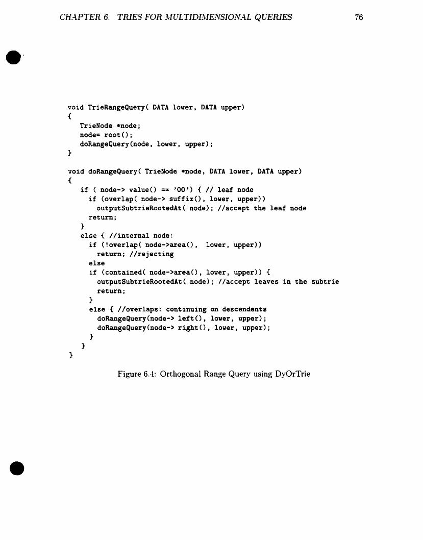
.'
•
CH..\PTER 6. TRIES FOR AJULTIDIAJE1VSI01VA.L QUERIES
void TrieRangeQuery( DATA lover, DATA upper){
TrieNode *node;node= root();doRangeQuery(node, lover, upper);
}
void doRangeQuery( TrieNode *node, DATA lover, DATA upper){
if ( node-> value() =z '00') { Il leaf nodeif (overlap( node-> suffixe), lover, upper»
outputSubtrieRootedAt( node); Ilaccept the leaf nodereturn;
}
else { Ilinternai node:if (!overlap( node->area(), lover, upper»
return; Ilrejectingelseif (contained( node->area(), lover, upper» {
outputSubtrieRootedAt( node); Ilaccept leaves in the subtriereturn;
}
else { Iloveriaps: continuing on descendentsdoRangeQuery(node-> left(), lover, upper);doRangeQuery(node-> right(), lover, upper);
}
}
}
Figure 6.4: Orthogonal Range Query using DyOrTrie
76
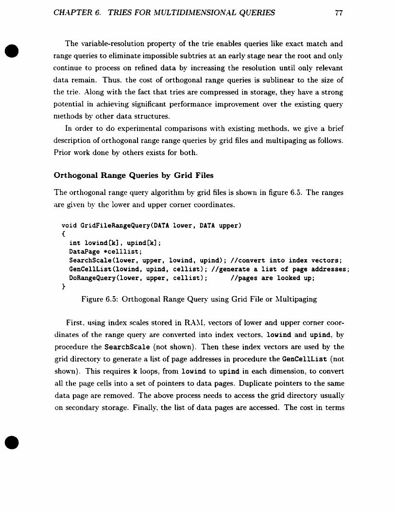
CHAPTER 6. TRIES FOR .l\;IULTIDIAIE1VSI01V:\L QUERIES 77
•
•
The variable-resolution property of the trie enables queries like exact match and
range queries to elirninate impossible subtries at an early stage near the root and only
continue to process on refined data by increasing the resolution untH only relevant
data remain. Thus. the cost of orthogonal range queries is sublinear to the size of
the trie. Along \Vith the fact that tries are compressed in storage, they have a strong
potential in achieving significant performance irnprovement over the existing query
methods by other data structures.
In order to do experimental comparisons \Vith existing ulethods, we give a brief
description of orthogonal range range queries by grid files and multipaging as follows.
Prior work done by others exists for both.
Orthogonal Range Queries by Grid Files
The orthogonal range query algorithm by grid files is shown in figure 6.5. The ranges
are given by the lower and upper corner caordinates.
void GridFileRangeQuery(DATA lo~er, DATA upper){
int lowind[k), upind[k];DataPage *celllist;SearchScale(lo~er, upper, lowind, upind); /Iconvert into index vectors;GenCellList(lo~ind, upind, cellist); //generate a list of page addresses;DoRangeQuery(lo~erJ upper, cellist); /Ipages are looked up;
}
Figure 6.5: Orthogonal Range Query using Grid File or ~'[ultipaging
First, using index scales stored in RA~I, vectors of lower and upper corner coor
dinates of the range query are converted iuto index vectors, lowind and upind, by
procedure the SearchScale (not shown). Then these index vectors are used by the
grid directory to generate a list of page addresses in procedure the GenCellList (not
shawn). This requires k loops, from lowind to upind in each dimension, to convert
aB the page cells into a set of pointers to data pages. Duplicate pointers to the same
data page are removed. The above process needs to access the grid directory usually
on secondaI)" storage. Finally~ the list of data pages are accessed. The cost in terms

•CHA.PTER 6. TRlES FOR NfULTIDIAJENSI01VA.L QUERIES
of disk accesses is loosely bounded by
le
II (upind[i] -lawind[i] + 1)i=l
and will be examined in the experimental section.
Orthogonal Range Queries by Multipaging
78
(6.1)
•
Range queries by multipaging share the first two stages of SearchScale and GenCellList
as those of grid files. The only difference is that GenCellList can be performed in
R.-\~[ and thus requires no time in our model, where only the number of disk accesses
count. But the DoRangeQuery is more complex than that of grid files because a data
page may have pointers to its overflow pages. The pseudo..code of DoRangeQuery
for multipaging is given in Figure 6.6. The cost of multipaging when distributions
are close to uniforrn is also bounded by Equation 6. L However, for pathological
distributions, overflowing pages couId lead to a visit of the entire data file.
6.2 Experimental Comparisons with Multikey File
Structures
In the following experiments, we address eosts against four parameters that may
affect performance. These four parameters are file size, distribution, dimensionality
and query selectivity. Costs studied inc1ude the number of disk page aceesses, access
time and storage costs. The file structures we are going to compare to are aIl suitable
for multidimensional data, including direct access methods (multipaging and grid
files) and logarithmic file structures (R-trees/R*-trees and their derivative X-trees).
6.2.1 Costs
The number of page accesses to the secondal1' storage are a straightforward assess
ment of query eosts. But in some situations, not aIl page aceesses require the same
amount of time. Counting numbers of page accesses becomes insuflicient and may

•CH.4.PTER 6. TRIES FOR l'vIULTIDIAJE1'lSrO./V•.:\L QUERIES 79
•
void DoRangeQuery(DATA lover, DATA upper, DataPage .cellHead){
DataPage .p= cellHead; IIp is head of the linklist of pagesvhile Cp is not null) {
DoRangeQueryOnAPage( lover, upper, p)j Ilprocess one page at a timep = p-> next; IIp points to the next data page member of the linklist
}}
void DoRangeQueryOnAPage(DATA lover, DATA upper, DataPage .p){
DataPage *q;Ilload data page pinto RAH and do a sequential search on the page:sequentialSearch(lover, upper, p);
Ilif p has an overflov page chain list, search them as vell:q= p-> linkto; Ilq point to the first member of the overflov page listwhile ( q is not null) {
if (!q-> visited(» Ilif the page has not been processedDoRangeQueryOnAPageCq); lIdo range query on the overflov page
q= q-> linkto; Ilgoto the next page of the overflov list}
}
Figure 6.6: Page Searching in Orthogonal Range Query using ~'!ultipaging

CH.-\PTER 6. TRIES FOR AIULTIDIAJE.N5IONA.L QUERIES 80
•
•
even be nlisleading. In the case of X-trees, supernodes are groups of nodes which are
accessed sequentially rather than directly. So for X-trees, we cite the access times.
The times are not nleasured directly because of operating system interference as weIl
as the existence of mernory buffers and disk buffers. Instead, time is calculated using
the parameters of our disk~ a Seagate Hawk 2XL Ultra SCSI 3 with an average seek
time and rotation time of 14.54 msec, and a read time (for 1KB of data) of 168J.lsec.
For sequential reads. the random seek time is omitted.
Another cost to he considered is storage. Tries compress data, as opposed to
aIl the other methods we have discussed in the context of this thesis. vVe will look
at the trie compression rate in subsection 6.2.8. On the other hand, grid files are
significantly dependent on the correlation among multidimensional distributed data.
and which in turn affects the amount of storage for grid directories. ~'[ultipagingalso
degenerates for exact match queries when there is a strong correlation among the data.
Section 6.2.7 in\'estigates this based on new models in characterizing distributions.
6.2.2 Data File and Algorithm Implementation
Data llsed in the experinlents are from several sources. vVe use uniform random
synthetic data, synthetic data with nonllniform distributions, as \Vell as data from
contour maps [E~[R} and the {J.S. Census TIGER data.
AlI trie. multipaging and grid file algorithms are implemented by the author.
The R*- and X-tree implementations are from the X-tree author Berchtold [BKK96}.
These are the implementations they \Vrote. and were run on their machine as weIl.
The black size of files on seconda~' storage \Vas set at 4096 bytes for aH tests unless
specified othen\·ise.
In aIl cases, results shown are averages of 50 ta 100 runs where applicable. AH
queries are on point data. Tries on shaped data are investigated and compared \Vith
an analytical model of R*-trees [TS96], which is beyond the scope of this chapter.

CH.-\PTER 6. TRlES FOR ~\t[ULTIDI1'lE1VSI01VALQUERIES 81
•
•
6.2.3 Parameters
There are four parameters that may affect the query cost: file size, dimensionality~
query selectivity and distribution.
The cost of tries~ R*- and X-trees are logarithmic to file sizes. Nlultipaging and
grid files are direct access methods and thus they are independent of file size in
general. Section 6.2.4 shows that direct access methods have greater speed in exact
match queries. But for range queries, tries outperform ail others.
The increase of dimensionality degenerates the R*-tree performance. One rea
son is due to the overlap of directories which increases rapidly \Vith the growing
dinlensionality of the data. The X-tree is designed to improve the R*-tree at high
dimensions using a hybrid organization of partial hierarchy and partial linear orga
nizations. Tries do not have the overlapping problem as that of the R-tree variants.
In section 6.2.6. we demonstrate that tries outperform R*- and X-tree for both exact
and range queries in various dimensions.
Selectivity is defined as the ratio of records retrieved by a query to the total
number of records in the file . .-\ range query is an example of high selectivity in most
cases. Section 6.2.5 will show that tries outperform aIl other data structures except
at very lo\v selectivities, such as an exact match quer)'.
The distribution of data in multidimensions, i.e.~ the way in which data correlate
across dimensions. significantly affects the perfol'nlance of multipaging and grid files.
Section 6.2.7 shows that tries are not affected entirely by pOOl' distributions in tel'ms
of speed and storage costs.
6.2.4 Speed versus File Size
Figure 6. 7~ 6.8, and 6.9 show how the cost of exact match queries varies with the file
size. Figure 6.7 shows the 20 result, and figure 6.8 displays the high 160 result. Tries
are compal'ed with X-trees~ and R*-trees in 160. .-\S X-trees contain supernodes which
use subsequent sequential searches among its directory search, a complete analysis
should also include time delay measures. Figure 6.9 shows the equivalent elapse time
spent on disk accesses .

CH.~PTER 6. TRIES FOR 1\t[ULTIDI~IENSI01V.4LQUERlES 82
.
1 (3.2)1
1
~1
//
/
1
1
1
/~1.00)
- (0.67)
0 0 ~0.50)
105 106
o-
... 0
""
Exact match: 0:z2, page size=1024, uniform data
""
R--tree
- - grid file
multipaging-DyOrTrie
8
2l~ - - - -0- - - - .....~ ...- - - - El - - - -~~~--~~-~~
ol--__........-'-- --........ -.....I_~ ..L____........_.L___..................J
100 10' 102 103 10"'records
Figure 6.7: Page :\ccesses vs. File Size, 20. Exact ~Iatch
•
Exact match: 0=16. page size=4096 bytes. uniform data10
2.----------------------------.
• X-trees- - R--trees- OyOrTries
o1
(2.9)1,
1
1
ci,
1
1
1
1, ,/
, .4)"
.;~---_.- ..../
/"",.
,/
".
100.~----_e:::----_e::------------------J
100 101
102 103 104
105
'records
Figure 6.8: Page .-\ccesses vs. File Size. 16D~ Exact ~Jlatch
•

CHAPTER 6. TRIES FOR l\;IULTIDIAJENSIOIVA.L QUERIES
102
Exact match: 0=16, page size=4096 bytes, uniform data
• 1
1
Re-trees 1
êi)- - X-trees 1 2.5}
~ - DyOrTries /li)
§. 1/
li)Il
~1 1
1li)
1 1Q)
8 1 1eu 1
1~ e'6 "c0
ë8-li)
Q) ;r------~ /ë ;'Q) ;'iU />"S /CTW /
;'
/
10110° 10' 102 103 10" 105
'records
Figure 6.9: Equivalent Access Times vs. File Size, 160, Exact ~'Iatch
83
•
Fronl these results. when the number of records exceeds a million, tries are slower
than multipaging by a factor of 3 and grid files by 1.5, simply because tries are log
arithmic and not direct access structures. However, comparing \Vith tree-like struc
tures, tries outperform R*-trees by factors of 3.2 at 106 records in 2D. In 160, tries
are 2.9 times more efficient in page accesses using 105 records, and outperform X-trees
at 5 x 1001 records by 2.5 when considering the total time spent on disk accesses.
\Vhen file sizes increase, the trend is that trie costs increase logarithmicly, however,
tries supercede R*-trees and X-trees by greater degrees in exact match queries. This
is because R*-trees and X-trees performance deteriorates when files are bigger in high
dimensions. It is difficult for R*-trees to find overlap-free partitions when files are
\'ery big, and thus they have more overlapped directory pages ta be searched. The
X-tree tends to rail building hybrid hierarchy structures when there are an increasing
number of records in a file. Instead, the whole structure generates more and larger
supernodes, especially near the foot. These supernodes near the root are more likely

CH.4PTER 6. TRIES FOR !\IULTIDI1\JE1VSION.4.L QUERIES 84
•
•
to he visited during a query. This results in a sequential search of most of the file
instead of a tree search. In fact, it is exactly this reason why in figure 6.8, when
the number of records exceeds 103 , R*-trees have an improved ahility over X-trees
in terms of the number of page accesses; R*-trees have overlapped directory pages
to be visited, while X-trees have to search sorne supernodes· which further increase
costs. On the other hand, in terrns of time spent on these disk accesses, X-trees do
sequential searches on those supernodes, which save considerable amount of access
time to secondary storage. This is why in figure 6.9, the time delay search costs of
X-trees are lower or no \Vorse than that of R*-trees when files are larger than 103
records in 16D.
For orthogonal range queries, figures 6.10, 6.11 and 6.12 give the same set of
conlparisons at 0.2 selectivity for 2D and 160 respectively. Cost increases linearly,
along with the nUlllber of records, briefly for aU structures, bath in 2D and 160,
when there are enough records. Tries are superior to aU other structures. In 20, tries
outperform R*-trees by a factor up to 5.3, and irnprove performance over grid files
and multipaging by a factor of 1.9 and 2.1 respectively at 106 records. In 160 , tries
outdistance both R*-trees and X-trees up ta a factor of 2.2, at 105 records.
The major reason for the enhanced performance of tries over other structures is on
account to the storage compression they achieve. In fact, tries compress data while
other methods add storage overhead which in summary accounts for the result. \Ve
look further at the compression rate of tries in section 6.2.8.
6.2.5 Speed versus Selectivity
In this section. we give two groups of figures for the query cost versus the selectivity
for the contour and TIGER data, one in 20 and the other in 160. The selectivity plays
a principle role in the query cost for aU data structures. The higher the selectivity
is, the higher the query cost for any structure. Figures 6.13, 6.14 and 6.15 show that
tries outperform aU other methods, surpassing R*-trees, grid files and multipaging by
factors 5.5, 3.L and 2.1 respectively at 100% selectivity in 2D.
·One supernode contains a number of regular nodes. thus counts for more than a page.
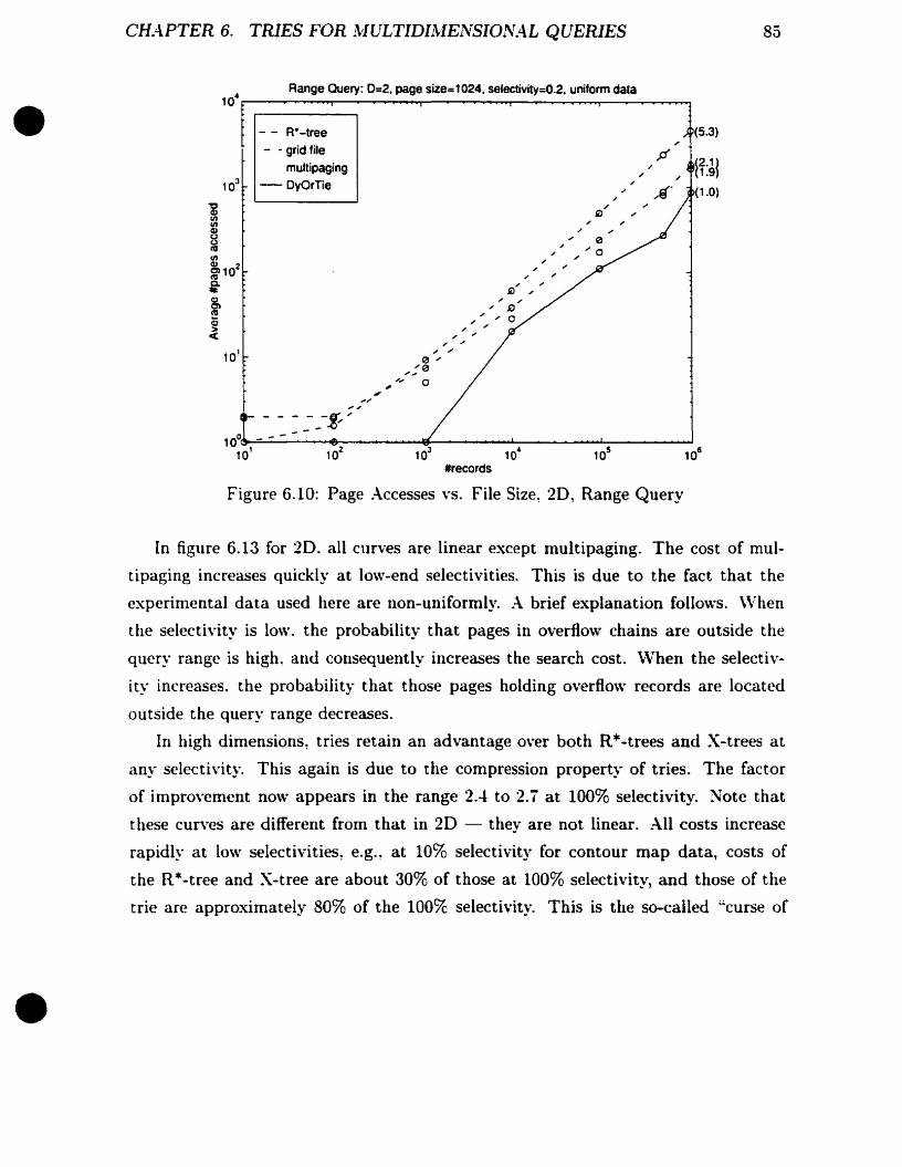
CH.4.PTER 6. TRIES FOR 1\tIULTIDINIENSI01V.4L QUERIES 85
Range Ouery: 0=2, page size=1024, selectivity=O.2. uniform data10
4C--~""""""""""'~-""""""""""-'--~----'-"""""'''''''''''''r----..................~-.....-. .......................,• - - Re-tree
- - grid file
multipaging
-OyOrTIe
- - - - - --"g:. '"100 - - - - -
10' 102
", ",
" "", '"
0'""'0
"''',,"''' 0
#records
",
•
Figure 6.10: Page :\ccesses vs. File Size~ 20, Range Query
In figure 6.13 for 20. aU curves are linear except multipaging. The cast of mul
tipaging increases quickly at low-end selectivities. This is due to the fact that the
experimental data used here are non-uniformly. :\ brief explanation follows. \Vhen
the selectivity is low. the probability that pages in overflow chaios are outside the
query range is high. and consequently increases the search cost. When the selectiv
ity increases. the probability that those pages holding overflow records are located
outside the query range decreases.
In high dimensions, tries retain an advantage over both R*-trees and X-trees at
any selectivity. This again is due to the compression property of tries. The factor
of improvement now appears in the range 2.4 to 2.7 at 100% selectivity. Note that
these cun-es are different from that in 2D - they are not linear. :\.11 costs increase
rapidly at low selectivities, e.g.~ at 10% selectivity for contour map data, costs of
the R*-tree and X-tree are about 30% of those at 100% selectivity, and thase of the
trie are approximately 80% of the 100% selectivity. This is the so-called "curse of

CH.-tPTER 6. TRIES FOR JIULTIDL\JEl'iSI01VAL QUERJES 86
Range Query: 0=16, page size=4096 bytes, selectivity:o: 0.2, uni.orm data104
r----~~---.-..........................---.---.-----.............~----.------.-.......-r---------"'T"""'O' ............,
#" (2.2)
(1.0)
- - X-trees- - Re-trees- DyOrTries
q
""... ", ,... "
"",,"""",
o ~", ' ...0, ..
, :::: - "'",._ ........... -
100~;;...""".,--,~__.L...- --..l ~"""""' -...J
101 102 103 104 105
#records
101
•
Figure 6.11: Page .-\ccesses \·s. File Size~ 16D~ Range Query
dinlensionality~·. For simplicity. assunle the query range is a hypercube. \-Vith the
selectivity at 10%. the sicle length in a dimension is 0.1 l/16 = 0.87 in a data space of
a 16D unit hypercube [O. 1) 16. This is larger than three-fourth of the space in that
dimension. \Ve know that tries always partition the space into two haU subspaces.
This means that at least the first 2 x 16 + 1 = 33 levels of the trie nodes need to be
\·isited. A complete trie with 33 levels of nodes can hold up to 232 = 4 billion records.
Thus~ with 6 x 10⁴ records in the contour map file, 33 levels of nodes certainly means
most pages of the trie. For the R*-tree and the X-tree~ the data space is split only
once in a number of dimensions. It is not split at all in the remaining dimensions,
and thus the bounding boxes of the pages include almost the whole extension of the
data space in these dimensions. For example~ if a 160 data space has been split
exactly once in each dimension~ it would require 216 = 65536 data pages, and we have
only less than 2000 pages for bath the R*-tree and X-tree. On the other hand~ it
is intuitively clear that a query with sicle length of 0.87, must intersect with every
•
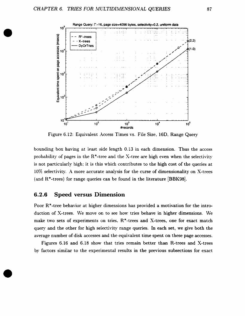
CH.-\PTER 6. TRIES FOR 1\IULTIDIAIE1VSION.4L QUERlES 87
Range Ouery: r=,16, page size=4096 bytes, selectivity=0.2. uniform data, 05
...-:-----.-----.--.....................y-~~-.-.-.......-r- ...........--.......................,....-~--- ..........~.....,
. ; (2.2)
,,./'
, ,.,./q
"'...
- - R·-trees- - X-trees
- DyOrTries
10''''-------~-----...I.-------...I.-------..-.....J
la' 102 103 10· 105
"records
•
Figure 6.12: Equivalent Access Times vs. File Size, 160, Range Query
bounding box having at least side length 0.13 in each dimension. Thus the access
probability of pages in the R*-tree and the X-tree are high even when the selectivity
is not particularly high~ it is this which contributes to the high cast of the queries at
10% selectivity. A more accurate analysis for the curse of dimensionality on X-trees
(and R*-trees) for range queries can be found in the literature (BBK98].
6.2.6 Speed versus Dimension
•
Poor R*-tree behavior at higher dimensions has provided a motivation for the intro
duction of X-trees. \Ve move on to see ho\\" tries behave in higher dimensions. vVe
make two sets of experiments on tries, R*-trees and X-trees, one for exact match
query and the other for high selectÏ\'ity range queries. In each set, we give both the
average number of disk accesses and the equivalent time spent on these page accesses.
Figures 6.16 and 6.18 show that tries reroain better than R-trees and X-trees
by factors similar to the experimental results in the previous subsections for exact
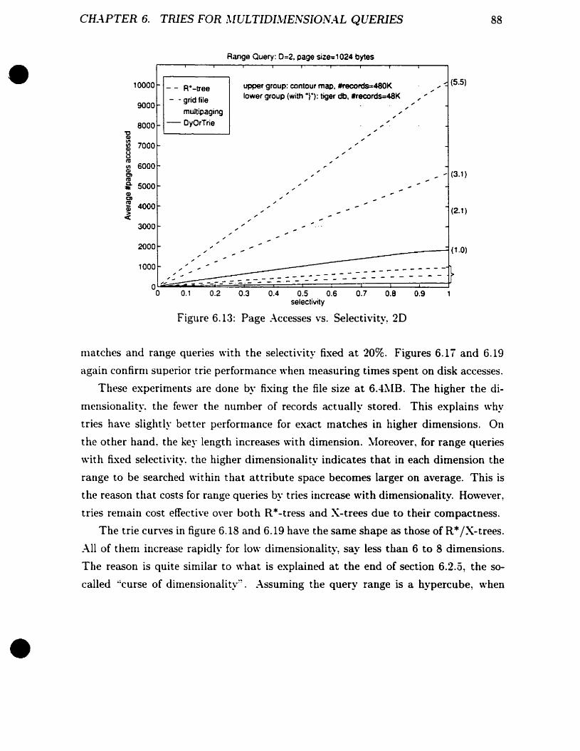
CH.-\PTER 6. TillES FOR ~\[ULTIDI:.\JE1'lSION.4L QUERIES 88
• 10000
9000
8000
- - R--tree
- - grid file
multipaging
- DvOrTrie
Range auery: 0=2. page size=' 024 bytes
upper group; contour map, trecords=480Klower group (with -}"); tiger db, trecords=48K
(5.5)
ocCDlI'l
7000lI'lCD
~calI'l 6000CD (3.1)0) -cai- 5000CDCl
t! 4000CD (2.1)><3000
0.9
---_ .... ---
0.8
- - - - - - - -
0.70.30.2 0.4 0.5 0.6selectivity
Figure 6.13: Page :\ccesses vs. Selectivity~ 2D
o 0.1
1000
2000
nlatches and range queries with the selectivity fixed at 20%. Figures 6.17 and 6.19
again confirnl superior trie performance when measuring times spent on disk accesses.
These experiments are done by fixing the file size at 6.4~IB. The higher the di
mensionality~ the fewer the number of records actually stored. This explains why
tries have slightly better performance for exact matches in higher dimensions. On
the other hand. the key length increases with dimension. ~'1oreover~ for range queries
with fixed selectivity~ the higher dirnensionali ty indicates that in each dimension the
range to he searched within that attrihute space becomes larger on average. This is
the reason that costs for range queries by tries increase \Vith dimensionality. However,
tries remain cost effective O\'er both R*-tress and X-trees due to their compactness.
The trie curves in figure 6.18 and 6.19 have the same shape as those of R*/X-trees.
AIl of them increase rapidly for low dimensionality~ say less than 6 to 8 dimensions.
The reason is quite similar to what is explained at the end of section 6.2.5, the so
called ~;curse of dimensionality~~. .-\ssuming the query range is a hypercube~ when
•
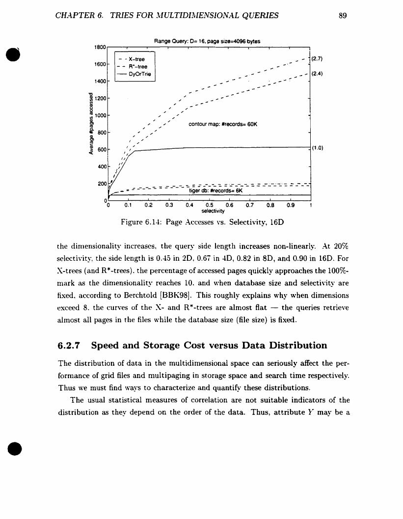
CHAPTER 6. TRIES FOR ~\fULTIDIllIENSI01'l.4.LQUERJES 89
• 1600
1400
- - X-tree- - A--tree- DyOrTrie
Range Ouery: 0= 16. page size=4096 bytes
_ - (2.7)
(2.4)
contour map: Irecords= 60K
~
~ 1200enCIl
~~ 1000CIlClIls
i' 800 ~CIl
g' "J~.!;"~~~~~~~~~~~~~~~~~~~~~(1~)
/1
200-' _ - --- - -.- - _.- - --_.--- _._--f, _ - - -=-:: :----- -=. - - - - - - - - - - - - - - - - - - - - - -
_ - GO - - - - tiger db: 'records= 6K
0.1 0.2 0.3 0.4 0.5 0.6selectivity
0.7 0.8 0.9
•
Figure 6.1--1: Page .-\cccsses vs. Selectivity, 16D
the dirnensionaIity increases~ the query side length increases non-linearly. At 20%
selectivity~ the sicle length is 0.-15 in 2D~ 0.67 in 4D, 0.82 in 8D, and 0.90 in 16D. For
X-trees (and R*-trees). the percentage of accessed pages quickly approaches the 100%
nlark as the dinlensionality reaches 10. and when database size and selectivity are
fixed, according to Berchtold [BBK98]. This roughly explains why when dimensions
exceed 8. the curves of the X- and R*-trees are almost fiat - the queries retrieve
alrnost aIl pages in the files while the database size (file size) is fixed.
6.2.7 Speed and Storage Cost versus Data Distribution
The distribution of data in the multidimensional space can seriously affect the per
formance of grid files and multipaging in storage space and search time respectively.
Thus we must find ways to characterize and quantif:~' these distributions.
The usual statistical measures of correlation are not suitable indicators of the
distribution as they depend on the arder of the data. Thus, attribute Y may be a

CH.4PTER 6. TRIES FOR AfULTIDll\JE1VSI01V.4.L QUERlES 90
20000 .----y----r---r---,-------r--~-~--r---~-___,Range Ouery: 0= 16. page size=4096 bytes
• 18000
ûi"(.)
~ 16000§.en~ 14000en(1)
~ 12000JI:.en'6g 10000 ~
- - X-tree- - R--tree
- DvOrTrie
.-
contour map: 'records: 60K
_ (2.6)
(2.4)
c ' ;(1) " ,,"
fi- 8000 ~ " "(1) 1,,:..-"_------------------,(1.0)
i:::(,/'Lff l,
2000 __-_--":. = =_-_-_~ =..:--~-- -=. =------- =. =-----"":... ==--.:..--.._ - ~ - tiger db: 'records::: 6K
0.90.80.70.30.20.1 0.4 0.5 0.6selectivity
Figure 6.15: Equivalent .-\.ccess Times vs. Selectivity, 16D
function of attribute .\! Y = f(x), but the statistical correlation between .Y and }
will be quite different depending on \Vhether f is a straight Hne or f has points which
are distributed uniformly across the plane.
"oe turn to information theory and find that the information-theoretic correlation,
which we will from now refer to as correlation for simplicity! provides an excellent
measure for the behavior of multipaging. Similarly, the mutual information, which we
will from now on refer to as information, is a good indicator for grid files performance.
For random variables .\. Y, ... , Z \Vith probability P(Xi, Yj' ...• Zk), and .\ = Xi,
} - = Yj ... Z = Zk. the information is
Ix}·...z = L P(Xi, Yj, ... , Zk) logp(xi, Yj, ... , Zk)ij ...k
The correlation is given by the expression
I.·o ·...z - lx - Iy - ... - Iz
•
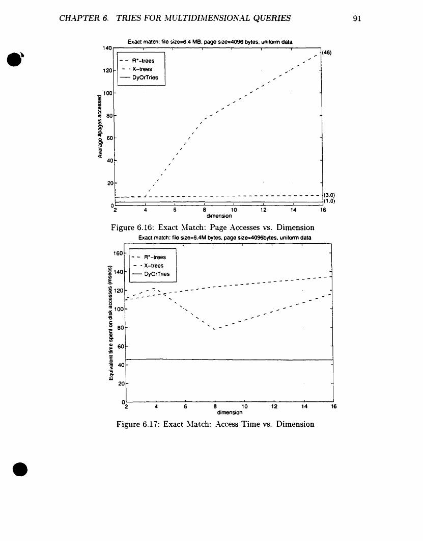
CHA.PTER 6. TRIES FOR 1vIULTIDI1\JE1VSI01VAL QUERIES
Exact match: file size=6.4 MB. page SiZ8=4096 bytes. unitorm data140...----...---~----r----...---"'"T'""---...J---...,
(46)
91
120
- - Re-trees_. - X-trees
- DyOrTries
100 ..ili)li)Q,l
8 80ca."
li)Q,l
iQ. 1•Q,l 60~ /
C)
eQ,l:>4(
40
20~
f---- - - ~ - - - - - - - - - - - - - - - - - - - - - - - - - - - - - - - (3.0)
C::====::i::====::::L:====::::::;:======:L::::::====:::C=====:::i:====:::j(1.0;°2 4 6 8 10 12 14 16
dimension
Figure 6.16: Exact ~'(atch: Page Accesses vs. DimensionExact match: file siZ8=6.4M bytes. page siz8z 409Gbytes. uniform data
160- - Re-trees
en - - X-trees~ 140.. - DyOrTries§.en~ 120 - ...... ---:;:-~ .:'--- -~ 100'6c:~ 80~c:§.
- - -
,
----- - - - ----------
.-
-
-
•
Q,l60~
~ëlU(ij 40~>"3CT~
20
O2 4 6 8 10 12 14 16
dimension
Figure 6.17: Exact ~latch: Access Time vs. Dimension

CH.-\PTER 6. TRIES FOR 1\;fULTIDI1\JE1VSI01V.4L QUERIES 92
2500Range query: file size=6.4MB.page size=4096 bytes.selectivity=0.2.unitorm data
__-_-- ~ ;:- t~:6~
1614128 10dimension
- - - -.:--- :: '- -- : =--
__----------1(1.0)
64
- - Re-trees
- - X-trees
- DyOrTries """""F" """".""
""" "" """"
""" "
" """1
"1N
1"
1"·1
Il
"Il
1000
2000
Figure 6.18: Range Query: Page Accesses vs. Dinlension
Range query: tile size=6.4MB,page size=4096 bytes.selectivity=0.2.uniform data
22.0)
20.6)
(1.0)
- - Re-rrees - -- -(- -- -- - X-trees - - (~ - - - - - - -- - - - -- DyOrTries - - -- - - - -- - - - - - -,,- - -
""""~
1/
/.. ,,",
,",,'
" ".."1
/"1/1
V- 'i
'"//
40000
cn35000c.,)
~§.~30000enenID
~~25000'6co
1.20000
ID
:§E 15000ID(ij>"3r:rw 10000
4 6 8 10dimension
12 14 16
Figure 6.19: Range Query: Access Times vs. Dimension
•

CH.-\PTER 6. TRIES FOR AIULTIDll\IElVSI01V.-\L QUERIES 93
• The correlation vanishes only when the distribution of .Y, }~, ... , Z is the product
of the distributions of the individual fields. This is referred to as a Cartesian product
distribution. The correlation reaches its maximum when every pair of variables forms
a function..-\ Cartesian product distribution is ideal for multipaging. On the other
hand: functional dependencies produce pathological distributions. An example of such
is a circular distribution. which also has a high correlation. Therefore, we consider
the correlation as a good predictor of multipaging performance for access times.
The information is minimal when the probabilities are aH equal and the distri
bution is uniformt. The information is maximal when aU probabilities but one are
zero. and the distribution is sharp. This happens exactly wh~n the grid file directory
has to waste the most space. Thus we can use the information to predict grid file
directory space costs.Storage consumption :D::2,page size::1024 bytes,synthetic data.#records=1OOOk
4,....------r-----r------r----r------r----.------..--,
3.5
0.5
• X-tree
RO-tree
- - grid file
multipaging
- DyOrTrie
. - - - -------__-- -- l! _ - - - - - - - - - - -"_:1'
. ,..
- - "/'"" ,,,,
, (12.8)
',. • (5.7)- - - (5.4)
(3.7)
-- (1.0)
•
O'--__.....J.... .l--__--l- ....l.....-__--L. ....I....-__--J.~
-14 -13 -12 -11 -,0 -9 -8 -7Ixy at resolution level of around grid level
Figure 6.20: Storage Cost \'s. Distribution
tXote that we are using the negative of what is normally called "information" and which is ma.'Cimum for uniform distributions. This is to make the consistency that low values always correspondta good performance.

CHA.PTER 6. TRIES FOR }/ULTIDIlvIE1VSI01V.;.\L QUERIES 94
18r-------r---,----~---yo---,.....--~----'T--~-___.,. (6.0)Exact match: 0=2. page size=1024 bytes. synthetic data. 'records=1000k
• 16- • X-tree- - R·-tree
14 - - grid file
multipaging
l12 - DyOrTrielit
§: 10 r-& l' ~ -- - ... - - - -a. ...!! - - - - - - - -.- - - -• 8r-G)
~
l 6~
4
•------ - (2.7)
1----------------------------;(1.0)
2-·- - -'-'- - _.- _.- _._._._.- _.- _.- _._._.- - _.- -'- --- (0.7)
0.5 1 1.5 2 2.5 3 3.5Correlation at resolution level of around grid level
4 4.5
•
Figure 6.21: Exact ~'[atch: :\.ccess Cost vs. Distribution
It can be nlisleading if we measure information and correlation based on each indi
vidual record location. For instance, }' might be a function of .\ and the correlation
is at a nlaximum. and thus the predicated performance of nlultipaging is very poor.
But this function could be such that every page of a multipaging space is unifornlly
occupied, which results in optimal performance. :\.s we count costs in terms of disk
pages/blocks on secondary storage. we measure the probabilities for page locations.
i.e., aggregated over pagefuls of records! in the following experiments.
To test the effects of data distribution, we use a 2D synthetic data with distri
butions ranging from Cartesian product to functional straight lines, each with 106
records and a page capacity of 1024 bytes.
:\. poor data distribution affects the storage of grid files, but does not bother
tries or multipaging. Thus, we use infornlation as a measure of the distribution
in Figure 6.20 ~. ~[ultipagÏng requires a small storage overhead. The trie gains
tThe correlations as defined are negative. and to help intuition, we double the negative.

CH.-\PTER 6. TRIES FOR 1\JULTIDI1\fE.l'lSION.-\L QUERIES 95
•
•
compression due to the overlap of paths near roots. The grid file starts with a 50%
overhead! and it rises ta 350% as the distribution quality declines. This is mainly due
to the expansion of the grid directory. The R*- and X-trees have overheads that faH in
the range of 130% to 300%. But apparently they do not depend on the information.
Figure 6.21 shows the effect of the data distribution on access costs. ~Iultipaging
is the only data structure which shows a dependency, and thus the correlation is used
as a measure of the data distribution§. For a good distribution (correlation is 0),
illUltipaging demonstrates the best performance at one access, follawed by grid files
and tries~ at a constant two and three aceesses respectively! at this particular nurnber
of keys.
R-trees and X-trees retain higher access costs than the other methods, but are
unaffected by the data distribution in general. R-trees have higher access costs be
cause of the overlaps of rectangles causing more pages than necessary to be searched.
The costs of X-trees are very similar to R-trees since we count a super node access
as equivalent to many regular page accesses. however, recall that the linear accesses
can in fact reduce the costs in tinle ta those less than that of R-trees.
The cast of multipaging degenerates quickly, while others are remain stable for
different distributions.
6.2.8 Data Compression versus Storage Overhead
One of the main reasons that tries obtain an advantage over other methods for exact
nlatch and range queries rests on the fact that it compresses data. \Ve define the
file compression rate as the ratio of the size of the compressed file to the size of the
original data file. Figure 5.1 in chapter 5 shows that the file compression rate becomes
less than 0.1, i.e., over 90% of the file size has been reduced! for large files in 10.
In addition, the data compression also depends on the size of a data record (if we
assume that every attribute of a record consumes the same space! then the size of a
data record is determined by its dimensionality as weil). Figure 6.22 shows how the
§The absoiute value ranges from 0 to a maximum, which depends on the size of the data set.The range is not significant .
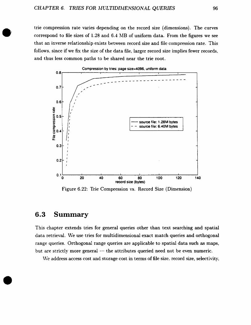
CHA.PTER 6. TRIES FOR AIULTIDI1\JE1VSIONA.L QUERIES 96
• trie compression rate varies depending on the record size (dimensions). The curves
correspond to file sizes of 1.28 and 6.4 ~IB of uniform data. From the figures we see
that an inverse relationship exists between record size and file compression rate. This
fol1ows, since if we fix the size of the data file, Larger record size impLies fewer records,
and thus Less common paths to be shared near the trie root.
Compression by tries: page size=4096, uniform data0.8 r-------r----r-----.--------,------r-----r------,
- source file: 1.28M bytes- - source file: 6.40M bytes
------------------- - -0.7
'"'"1
0.61
1
Q)1
! 1
1
.§ 0.5 1li) 1li)
! 1~ 1E8 0.4 1
1~ 1Li:
1
0.3,1
1
1
1401201004020 60 80record size (bytes)
Figure 6.22: Trie Compression vs. Record Size (Dimension)
6.3 Summary
•
This chapter extends tries for general queries other than text searching and spatial
data retrieval. \Ve use tries for multidimensionaL exact match queries and orthogonal
range queries. Orthogonal range queries are applicable to spatial data such as maps,
but are strictLy more general - the attributes queried need Dot be even numeric.
\Ve address access cast and storage cost in terms of file size, record size, selecthity,

dimensionality and distribution. Our experimental results show that tries are superior
to aU other structures (both direct access methods represented by multipaging and
grid files~ and tree structures including B-trees, R-trees/R*-trees and X-trees) in
queries returning more than a few records. ~Ioreover, tries are competitive with
direct access method in exact match queries.
Cnlike multipaging which cao deteriorate on search cost with pathological dis
tributions. and grid files which can \Vaste storage space on grid directories for bad
distributions. tries are unaffected by the data distribution.
For high dimensionality, tries are still up to 2 and 3 times better than R*- and
X-trees which \Vere invented for high dimensional spatial data.
Tries always compress data, resulting in savings for storage cost. This is in contrast
to grid files which consume large amounts of space for uneven distributions, and R*
trees and X-trees that use at least twice as much space as the sources. HoweveL it is
noted that multipaging does indeed have small space overhead as in the case of tries.
In facto trie compression is one of the two major reasons that tries achieve better
speed performance for queries returning more than a few records. This combines
with the variable-resolution property, enable tries to be a superior method for mul
tidimensional general data. Our task is to extend them to more general queries and
operations. In the next chapter. we will apply tries to relational join operations.
CHA.PTER 6. TRIES FOR AJULTIDIAJEiV5IONA.L QUERIES 97
•
•

Chapter 7
Relational Joins by Tries
\Ve have surveyed join algorithms in Section 3.3. Overall, to the best of our knowledge,
there has been no work on join algorithnls that takes advantage of existing data
structures, i.e., no extra indexes, for better join performance, and yet achicving spatial
conlpression at the same time.
In this chapter. we are \vorking on data sets organized by tries, not relations di
rectly. \Vith the buHt-in properties of order preservation on keys. storage compression
and \"ariable-resolution. tries have benefits Dot only in indexing large text data and
spatial data retrieval. but also in general database queries such as exact matches and
orthogonal range queries. In this chapter we extend them for even broader use to join
processïng"
\Ve tirst assume that the joïn attributes do not have duplicates, i.e., they are keys.
In this situation. joins are in fact set operations. Our inputs are two tries built on the
joïn attributes and the join result is a new trie. Based on the unique characteristics of
the data structure, there are a number of advantages that joins by tries can achieve.
1. The variable-resolution structure of the trie supports less than one pass search
cast in terms of the trie size. This happens in practice by making decisions
at la\\" resolutions near the root as ta whether a particular subtrie needs to be
visited or not for various unary Queries and binary joins.
2. The worst case cost of the trie join (TJ) algorithm happens when ranges of joïn
98
e
le

CHA.PTER 7. RELA.TI01VA.L JOINS BY TRIES 99
attribute values are totally overlapped, and that the output values organized by
the trie are as large as the input tries. In this case, complete traversaIs of bath
input tries have to be done. But due to the compression tries achieve, the cost
is still less than one pass of the original data sets without trie compressions.
Therefore the worst case join cost is linear with a leading coefficient which is
less unity. Note that we exclude the cost of the input trie construction and
sortïng.
3. Hash joïn methods do not r>reserve arder, which is indeed maintained by tries.
This property allows tries to be easily extended for efficient non-equijoins.
.-\mong them, union (unionL symnletric difference (xor), and difference joïn
(minus) operators will be considered in further discussions.
-1. \\llell there exist indexes on joining attributes, which is the situation in very
large databases~ the queries can make use of these indexes to achieve better
perfornlance. Our input tries have built-in indexes on joining attributes.
7.1 Joïn Algorithms by Tries
Binary tries for data sets Rand S in section 3.3.2 figure 3.5(a) are given ln fig
ure 7.1(a). The two sets in binary format are [00010~ 00011, 00100. 00101, OliOL
10000. 1000L 10010], and [00001, 00010, ... ~ Ollill respectively. Figure 7.I(b) shows
their corresponding OrTries. Our join algorithm performs synchronous~ depth-first~
post-arder traversaIs of the tries. First~ root Rodes of Rand Sare visited, and the
depth-first traversais lead to the first left leaf node of R and the second left leaf node of
S shown in figure i.l(b), with paths 10, 11, 11, 01, 11. The two nodes are compared
by an and operator~ 00 and 00, resulting in OO~ a new leaf Dode. Then, the jain visits
the right siblings and performs and operation on them, which results in a leaf node 00
as weIl. :\ext~ the post-order traversaI returns to the parent code 11. As it has bath
left and right children. the value 11 is made final. The post-arder traversai returns
back another level~ ta node 01, and it is made final as weIl, as it only has a right child
node 11. The post-order traversaIs of both trics continue. \Vhen the second nodes
•
•

CH.~PTER 7. REL.-\TIONAL JOINS BY TRiES
R
100
s •1111 1011011001101011Il 1101 Il 100000000000000000
10IlIl IlIl Il Il Il01 Il 11 Il Il Il 11 Il000000000000000000000000000000
(a) (Full) Tries for Set R and S
R S
rIlIl 101100(101}1O01 10 Il
I II Il 1100(01000000000000
10IlIl IlIl Il Il IlOO( 11 Il Il Il Il Il Il Il0000000000000000000000000000
lb) OrTrics for Set R and S (Shaded nodes arc the common nodes visited during the join process.)
10 1Il1100(101101 10
11 Il J00000000
(c) Resulting Trie after Natural Join of R and S
Figure 7.1: Joining Data Set Rand S by Tries
•

CH.4PTER ï. RELA.TIONA.L JOINS B}· TRIES 101
on the third levels, OO{ DID} and 11, are reached, with the former a leaf Dode and the
latter an internai node, and since the path 010 can also lead to a leaf on 5, a nlatch
is found and the join results in a leaf Dode OO{ 01 O}. Otherwise, the resulting node is
empty~ and we denote it by cjJ. If this happened, when returning to the parent node~
the corresponding offspring, right child in this case, should have been truncated; the
parent node should be changed to 10 from 11. \Vhen the traversais of Rand 5 return
to the roots, the output node lOis made final, and the join process is complete. The
shaded nodes in figure 7.1(b) give the common paths that ~.re traversed by the join
process. Other nodes have been skipped during the process. The output trie is given
in figure 7.1 (c) .
:\ow we summarize the trie join algorithrn from the above example; it is a syn
chronous. depth-first post-arder traversai of the two tries of input data sets. The
tran~rsal starts with the roots of the t\Vo tries, and moves down leveis in tandem until
there is no match possible in the subtries, or a leaf node is reached in one of then1.
At each step, the two nodes from t\Vo tries are compared. If the result is a match, the
corresponding subtries are then visited, resuiting in depth-first traversaIs. Otherwise.
when returning ta its parent node. this offspring shouid be removed in the output..
and the subtries rooted at these t\Vo nodes neecl no further visits. \Vhen two nodes
are first visited during the traversais, the logical and operation is performed on the
2-bit nodes. If the result is not 00 for internai nodes, it is a match. However, when
any leaf node OO{ remaining bits} is invoived, if the other node in comparison is also a
leaf Dode and their remaining bits are a match, or if it is an internaI node and a path
from the node to a leaf representing the same remaining bits, then it is still considered
as a match. In bath cases, OO{remaining bits} is the result of the join. Otherwise.
the resuit is a lnismatch and the path from its ancestor node must be truncated.
Table 7.1 is a binary table showing the result of the IOgÎcal and operator on t\Vo
nodes from the input tries, when they are first visited during the traversaIs. The first
column and the first row gÎve node values from the two input tries respectively. The
result is Rb, an abbreviation for remaining bits, if the two inputs match, eise empty!
denoted by d>. \Vhen the result is empty, it means that the link must be remo\'ed
from its parent node when the post-order traversai returns to the parent level. :\s a
•
•
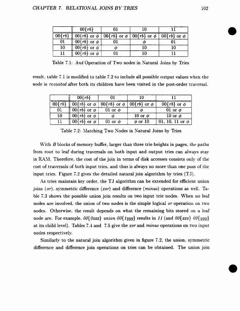
CH:\PTER 7. REL..4TIONA.L JOINS BY TRIES 102
OO{rb} OO{rb} or 4> OO{ rb} or 4J OO{ rb} or 4> OO{ rb} or <p01 OO{ rb} or 4> 01 ri> 0110 OO{rb} or ,p 4> 10 10Il OO{ rb} or l/J 01 10 Il
~ OO{ rb} 01 10 Il •Table 7.1: .4nd Operation of Two nodes in Natural Joins by Tries
result, table 7.1 is modified to table 7.2 ta include all possible output values when the
node is revisited after both its children have been visited in the post-arder traversaI.
il OO{rb} 01 10 IlOO{rb} OO{ rb} or f/J OO{ rb} or 4> OO{ rb} or l/J OO{ rb} or 4>
01 OO{ rb} or cP DIor cP cP DIor l/J10 OO{ rb} or cP 4> 10 or 4> 10 or 4>Il OO{ rb} or l/J DIor rP 4> or 10 01, 10, Il or 4>
Table 7.2: ~Iatching Two Nodes in Natural Joins by Tries
\Vith B blacks of rnemory buffer, larger than three trie heights in pages, the paths
fronl root to leaf during traversais on both input and output tries cao always stay
in RA~1. Therefore, the cost of the join in terms of disk accesses consists only of the
cost of traversais of both input tries, and thus is always no more than one pass of the
input tries. Figure 7.2 gives the detailed natural join algorithm by tries (T,J).
As tries maintain key order~ the T J algorithm can be extended for efficient union
joins (or). symmetric difference (xor) and difference (minus) operations as well. Ta
ble 7.3 shows the possible union join results on two input trie nodes. \Vhen no leaf
nodes are involved, the union of two nodes is the simple logical or operation on t\Vo
nodes. Otherwise, the result depends on what the remaining bits stored on a leaf
node are. For example. OO{ Oxxx} union OO{ lyyy} results in Il (and OO{xxx} OO{yyy}
at its child level). Tables 7...1 and 7.5 give the xor and minus operations on two input
nodes respectively.
Similarly ta the natural join algorithm given in figure 7.2, the union, symmetric
difference and difference join operations on tries can be obtained. The union join
•

•CH.-\PTER 7. REL.-\TION.4L JOllVS BY TRIES
BOOL NaturalJoinCTrieNode *tl, TrieNode *t2){
if( is_leaf(tl) or is_leaf(t2» {if(NaturalJoinOneLeaf (tl, t2» {~ite_a_leaf_node(tl)j Iloutput the leaf Dode to the resulting trie;return(TRUE)j
}
elsereturn(FALSE)j
}
node= 0; Il set tvo bits for the Dode to be 00if (both tl and t2 have left branches) {
if( NaturalJoin (tl-> left, t2-> left»Dode += 2j Il set tvo bits for the node to be 'lX'
}
if (both tl and t2 have right branches)if (NaturalJoin (tl-> right, t2-> right»
Dode += 1; Il set tvo bits for the node to be 'Xl'
103
}
if (node == 0)return( FALSE);
Il no match
•
vrite_a_node( node); Iloutput the node to the resulting trie;return (TRUE);
}
BOOL NaturalJoinOneLeaf(TrieNode -tl, TrieNode -t2){
if (is_leaf(tl) and is_leaf(t2»return (NaturalJoinLeaves( tl, t2»;
if (is_leaf(t2»return (NaturalJoinOneLeaf( tl, t2»; Iltl i5 the leaf node
Ilthere i5 only one path from node t2 that might match vith tlif ( cur_bit(tl) matches vith Dode t2 ) {
if ( is_leaf_level(t2) )return (TRUE);
elsereturn( NaturalJoinOneLeaf( tl, t2-> left»;
}
return (FALSE);}
BOOL NaturalJoinLeaves( TrieNode -tl, TrieNode *t2){
if (rest_bits_matchC tl, t2»return (TRUE);
return (FALSE);}
Figure 7.2: Natural Join Algorithm by Tries

•CHA.PTER i. REL.-\TI01V:\L JOINS BY- TRIES 104
OO{rb} 01 10 [TI]OO{ rb} OO{rb}, 01. 10 or Il DIor Il 10 or Il Il
01 DIor Il 01 Il Il10 10 or Il Il 10 IlIl Il Il Il Il
Table 7.3: ~Iatching Two Nades in Union Join of Tries
OO{ rb} 01 10 IlGO{ rb} dJ. 01, 10 or Il 4>.01 or Il (j), 10 or Il 01, 10 or Il
01 dJ. DIor Il <P or 01 Il 10 or Il10 ([J. 10 or Il Il (jJ or 10 DIor IlIl 01.10 or 11 10 or Il DIor Il ,p. DL 10 or Il
Table 7..1: ~Iatching Two Nodes in Symmetric Difference .loin of Tries
OO{ rb} 01 10 Il
•
OO{ rb} cP or OO{rb} 4> or OO{ rb} (jJ or OO{ rb} 6 or OO{rb}01 00 or 01 ,p or 01 01 cP or 0110 00 or 10 10 4J or 10 <t> or 10Il 01. 10 or Il 10 or Il DIor Il r/J, 01, 10 or Il
Table 7.5: ~Iatching Two ~odes in Difference Join of Tries

CHAPTER ï. RELA.TIOl'lAL JOnVS BY TRIES 105
•
•
algorithm is simpler than the other joins in the sense that there is no need to backtrack
and truncate paths from leaves to the root. The point is that tries are capable of
various binary join operations. In the following discussion~ we focus on natural join
as a representative of various join types which can be performed efficiently on trie
structures.
The above discussion on trie joins assumes that join attributes have no duplicate
values. In the presence of duplicates~ there are two different situations:
1. There exist non-join attributes, which are not indexed by the tries. This leads
ta a scenario where trie leaf nodes contain pointers to more than one record
stored on a separate file (or records share the sanie indexed attributes but have
different remaining attributes stored on a trie leaf).
2. There exist non-join attributes which are indexed on k-d-tries. This inlplies
that sorne trie node levels are non-join attribute bits and should be skippcd
during the join.
In the first case~ the joill algorithm rernains the same except at the end of the join
when leaves are reached: either pointers are used to point ta all remaining non-join
attributes corresponding ta many records on files, or these records have to be stored
on the leaf node themseh·es. \\te now partition the cost of joins into t\Vo pa.rts: one
for reading the input tries, and the other for writing the result to disk. Clearly, unlike
other join algorithms. the complexity of the first part of the T J algorithnl does not
increase, even though the size of the result increases. However, the cast of writing
the output trie to disk increases.
In the second case. the T J algorithm performs only on node levels representing
the joill attributes and skips others. The trie join becomes a many-forest join . The
same is true for ail other join algorithms. If duplicates can not be held within the
memory buffer~ the cost of the T J algorithm will be quadratic.

CHA.PTER ï. REL.4TI01V.4L JOllVS BY TRIES 106
• 7.2 Comparisons of TJ with Existing Jain AIgo
rithms
•
Sorne of the representative and state-of-the-art join algorithrns include the sort-rnerge
join (S~IJ), the distributive join (DJ), the join by fragment algorithm and the bucket
skip merge join (BSNIJ). However, since the T J algorithms use the built-in indexes
on joining attributes~ we assume the following for data sets in order to make fair
comparisons.
1. For S~IJ, both input sets are ordered according to join attributes. That is~ only
the merge phrase has to be carried out. Therefore we call it rnerge join (~[J)
frorn now on.
2. For DJ ~ both input data sets are already in order~ and the distribution table
has been built.
3. For BS~[J~ input sets are in arder and the bucket tables have been built up.
[t is pointed out and proven by Negri [NP91] that when input files are sorted
according to join attributes. the above join methods have the following relations:
1\JJ> DJ > JF
where .>' rneans more efficient than. Therefore it is true that T J is a more efficient
join algorithm than ~IJ~ DJ, JF and BS~IJ if only we can show that TJ is more
efficient than both ~IJ and BS~IJ for data sets ordered on join attributes. Thus, our
conlparisons become focussed on T,J, ~IJ and BS~IJ.
7.2.1 Best and Worst Case Analysis of TJ, MJ and BSMJ
Algorithms
The efficiency of a join algorithm is best characterized by the amount of disk accesses
required for the join processing. In this subsection, we analyze the best and worst
case in terms of disk accesses for T J, ~'IJ and BSNIJ .
CH.4.PTER 7. RELA.TIONAL JOllVS BY TRIES 107
•
•
The best case for the T J scheme occurs when there is no match at the top trie
levels, especially if the root pages do not match. In this instance, the total disk âccess
cost of T J is t\Vo pages. However, ~IJ and BSJ\IJ may still need to load aH the pages
for a possible match as ranges for the t\Vo datasets may fully overlap \Vith each other.
Therefore, this may still he the \Vorst case for the NU and BS~IJ schemes.
The best case for ~'IJ and BSJ\[J occurs \Vhen all values of the join attributes of
one set is less than (or greater than) that of the other set. In this case, ~IJ will
examine aH the pages of one dataset and only the first page of the other, Le.. ~Vs + 1
blacks. as the cursor moves only in one key set. BS~IIJ only needs to visit the bucket
tables, and no pages in the data set are visited. In fact, one bucket table page of set
R and ail bucket table pages of set 5, which correspond to lVs b/p pages. Assume a
file with 106 data itenlS of 8 bytes each, page size p = 4096 bytes and bucket table
entry size b = 20 bytes. Then :,Vs = 8 X 10⁶ /4096 = 1953, and the bucket table
size is 1953 x 20(1096 :::::: 10 pages. The best case for BSl\'IJ is to visit only the
bucket table for set S. plus the first bucket table page for set R. Thus the total
cost is about Il accesses. The upper bound for the cost of T.J in this situation is
Height(trie R ) + Height(tr-ieJ. wherc the height of the trie in pages is a logarithmic
function of the size of the data set. For a file \Vith several million data items, the
trie height can be as low as 3 pages. Thus a typical upper bouod of T J cost is about
2 x 3 = 6 pages.
The worst case of the T.J algorithm occurs \Vhen ail pages have ta be loadcd from
the disk. Of course. this happens when aIl the join attributes overlap. The saIne
situation also coincides with the worst case of the NIJ and BS~IJ schemes when ~IJ
needs to visit aIl data pages. and BS~IJ not only has to visit ail data pages but also
the eotire set of bucket tables.
Table 7.6 summarizes the hest and the \Vorst case cost for each join algorithm.
The hest case speed-up of T J can he orders of magnitudes improvement over ~IJ
and BS~IJ. It shows that even in the worst case, T J outperforms ~IJ and BS~IJ by
a factor of Ifr (assume r = r R = r 5), where r is the compression ratio of the trie
organization. This compression ratio is a function of the file size and the size of data
items! and it can he any value between 0 and 1 for data sets contaioing more than

•CH.;\PTER i. RELA.TI01VA.L J011'18 B}'~ TRIES
Case Join Aigorithm Disk Access CostBest case BS~IJ lVs ; + 1
~IJ lVS + 1TJ 2
\Vorst case BS~[J (1 + ~)(lVR + .Ns )~[J (1.VR + lYS)TJ TR1VR + Ts lVS
Table 7.6: Best and \Vorst Case Cast Summary for Join NIethods
108
•
a few hundred records. This means a speed-up by T J over ~/[J and BSN[J is no less
than one in the \Vorst case.
In the case of duplicate join attributc values~ nested black scan have to be applieci
for ail these join algorithms including the TJ scheme. The \Vorst case cost is quadratic
to the input relation sizes. But since tries organize data \Vith considerable compres
sion, the gain by a TJ scheme over other methods increases. Assume the cast of ~(J
by nested block scan is C 1.'12 • where C is a constant, and 1.'1 is the input relation size.
If wc assume the conlpression rate by trie organization is T, where 0 < r < 1. then the
size of the input tries is r.V and the cast by TJ is no more than C(TJ.V)2 = r'2C·.V2 .
Hence~ the T.I scheme still outperforms its competitors, and its cast is no more than
r2 of that of ~[J with nested block scan. The more tries compress data, the smaller
r is resulting in a nlore efficient TJ.
7.2.2 ExperiInental Comparisons
In this subsection we give and compare experimental results for TJ, ~[J and BS~IJ.
Two inlportant parameters for the tests are the join selectivity, defined as the ratio
of the overlapped range to the total input data range of an attribute, and the dataset
size. Thus \Ve have made t\Vo sets of experiments; one is disk access versus the join
selectivity, and the other is disk access with respect to input file size.
AIl test data sets are 2D random data uniformly distributed between [0, 1f. If
the join selectivity is p~ then the two joins sets are in the range of [0, (1 + P)/2)2 and
[(1 - P)/2.1f respectively. For example, if P= 0.4, the left set range is [0,0.7f and

CH.~PTER ï. RELAT101'1A.L J011'1S BY' TRIES 109
•
•
the right set range is [0.3, 1)2.
Figure 7.3(a) shows the cost of disk accesses \Vith respect to the join selectivity.
The dataset size is 500k records (4~1 bytes) for bath input sets. T J has the fewest disk
accesses, while BSNIJ and ~[J vie in their raIe as the most expensive. The starting
cost of ~IJ is the highesL since it has to examine at least one of the two input data
files, even when the files have no intersection at aH. The starting cast of BS:\IJ is
not as cast as ~IJ because it includes only the visits to bucket tables when the join
selectivity is zero. T J is the best among the three at P = 0, as it avoids visiting aU
the remaining files by making decisions at the root page levels. It can he observed
that aIl three schelnes are affected by the jain selectivity because when the selectivity
grows. more data items are involved in the join and the corresponding disk accesses
increase.
Figure 7.3( b) shows the speed-up of TJ over ~IJ and BSNIJ. The lower the join se
lectivity, the more T.J improves over the other t\VO methods. Even when the selectivity
is one, i.e., the t\Vo joining sets are fully overlapped, T J has a marked inlprOVenlent
over both ~IJ and BS:\IJ by a factor of 2. BS~IJ is hetter than NIJ when joïn selec
tivity is less than one. However, this is reversed when selectivity is one hecause of
the extra accesses to the bucket tables by BS~[J.
The added advantages that T J exhibits in terms of disk access can he explained
by the following points. Firstly, the compression property of tries makes the input
data sets organized by tries consume less space. Secondly, the variable-resolution
structure of tries enable T J to avoid sorne accesses to lower level (high resolution)
pages by making decisions at low resolution levels near the root. \Vhen the join selec
tivity is lo\\", the variable-resolution property is the primary reason for the enhanced
performance over the other t\Vo join algorithms. \Vhen the join selectivity is high.
the compression property becomes the major factor for the improvement.
T J scales very well with respect to the size of the input sets; the scalability of the
algorithm is compared in figure 7.4. The join selectivity is fixed at 0.4 for these tests.
Figure 7.4(a) shows the cost of joins in terms of disk accesses when the file size varies
from 100 records to 106 records. The abscissa represents the file size as indicated by
the number of records in each input data file. Both the abscissa and ordinate are

6000
7000
•CHA.PTER 7. REL.-\TI01VAL JOINS BY TRIES
20 random uniform data, SOOK records X2. page size=1024 bytes8000r---~-"---r--"---r--"------r---"---r--,----'_ f~:8J
rn-4(- -: ~ -,--
---- ~~MJ _:lt'" - - - - ,+...
-TJ... )e" .....+.....
13000:'1
Z
2000
1000
110
o 0.1 0.2 0.3 0.4 0.5 0.6 0.7 0.8Joïn Selectivity Between Two Input Data Sets
(a) Cast in terms of disk accesses
0.9
2D random uniform data, SOOK records X 2, page size=1024 bytes
- - speed-up over MJ- - speed-up over BSMJ
" .
,
, ,, ,
~-"'X- ---+- -
- =~ -----.: : ~-~--- _.~--
•100 l..-_----I.__~__.....I....__ ___I~_ ____L__~__.L__ __I_____L._ __J
o 0.1 0.2 0.3 0.4 0.5 0.6 0.7 0.8 0.9Join Selectivity Setween Two Input Data sets
(b) Speed-up (disk accesses) ofTJ
Figure 7.3: Disk Accesses versus Join Selectivity
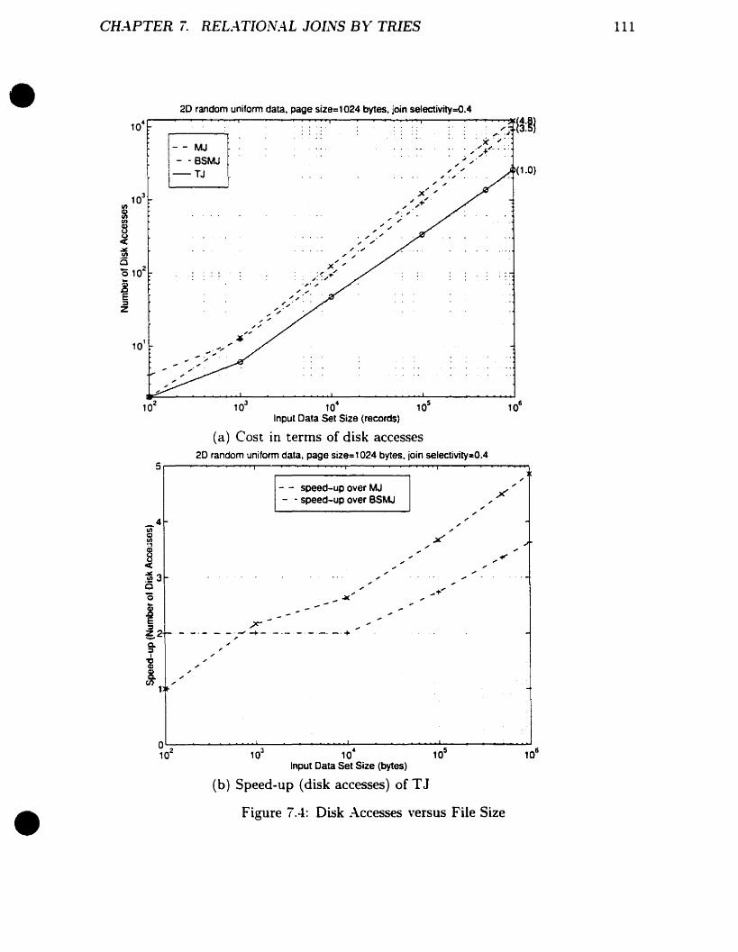
•CH.4PTER i. REL.4TIONA.L JOIl~S BY' TRIES
2D random uniform data, page size=1024 bytes. join selectivity=0.4
111
10"
10'
œ-MJ- - BSMJ-TJ .
. ", f3:~J. ~ - ".JI. )( r
:,':f"-- :" ., ,
,~,' (1.0), ,
;x' ,
,",+"". ,,', .;
,"-'. '" .'", ,
"',', '",:x '
,::.-+'""- "
"'""','-,'"',, ", ...
",~."
•
102 103 10" 105 106
Input Data Set Size (records)
(a) Cast in terms of disk accesses20 random uniform data. page size=1024 bytes, join selectivity=O.4
- - speed-up over MJ- - speed-up over BSMJ
t T~ ._._._- --,--'-+- --- -'_.-. _.+~:::)1
ic%1
OL.-~--_ ............L..._-_---..-...........L_-~----.-... ............-._---_......J1~ 1~ 1~ 1~ 1~
Input Data Set Size (bytes)
(b) Speed-up (disk accesses) ofTJ
Figure 7.4: Disk Accesses versus File Size
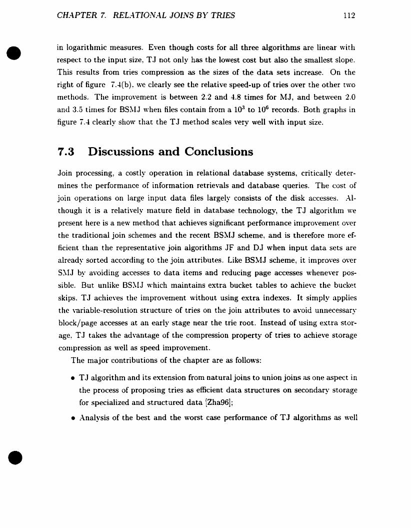
CH.o\PTER 7. RELATI01'l.o\L JOINS BY TRIES 112
•
•
in logarithmic measures. Even though costs for aH three algorithms are linear \Vith
respect to the input size~ T J not only has the lowest cost but also the smallest slope.
This results from tries compression as the sizes of the data sets increase. On the
right of figure 7.-1(bL we clearly see the relative speed-up of tries over the other two
methods. The improvement is between 2.2 and 4.8 times for l'vIJ, and between 2.0
and 3.5 times for BS~IJ when files contain from a 103 ta 106 records. Both graphs in
figure 7.-1 clearly show that the T J method scales very weIl \Vith input size.
7.3 Discussions and Conclusions
Join processing, a costly operation in relational database systems, critically deter
mines the performance of information retrievals and database queries. The cast of
join operations on large input data files largely consists of the disk accesses. .-\1
though it is a relatively mature field in database technology, the T J algorithul we
present here is a new method that achieves significant performance improvement over
the traditional join schemes and the recent BS~'lJ scheme, and is therefore more ef
ficient than the representative join algorithms JF and DJ when input data sets are
already sorted according ta the join attributes. Like BSwlJ scheme, it improves over
Sj.IJ by avoiding accesses to data items and reducing page accesses whenever pos
sible. But unlike BS~IJ which maintains extra bucket tables to achieve the bucket
skips. T J achieves the irnprovement without using extra indexes. It simply applies
the variable-resolution structure of tries on the join attributes to avoid unnecessary
block/page accesses at an early stage near the trie root. Instead of using extra stor
age, T J takes the advantage of the compression property of tries ta achieve storage
conlpression as weil as speed improvement.
The major contributions of the chapter are as follows:
• TJ algorithm and its extension from natural joins to union joins as one aspect in
the process of proposillg tries as efficient data structures on secondary storage
for specialized and structured data (Zha96];
• :\nalysis of the best and the worst case performance of T J algorithms as weIl

CH.-\PTER ï. REL.-\TIOiVAL JOINS BY TRIES 113
•
•
as competitive join algorithms ~IJ and BS~IJ;
• Detailed performance tests which show the superior performance improvement
of T J over BS~IJ and ~IJ ~ and thus show the superiority over the inlproved
hash join method JF and the improved merge join method DJ when input sets
are ordered.
So far we have assumed that the join attributes of the input data files are keys
stored on trie structures. If the input data files are not organized by tries or the
join attributes are not stored as keys on trie structures, we need to build tries on
these join attributes before performing the join. The construction of a trie from an
unordered input data seL like the construction of any other index structure~ has a
cost of l.V 10g(~V), where ..v is the number of keys. Thus, it remains an open research
problcm whether in this case joins by tries would still outperforrn existing join al
gorithms. ~evertheless. detailed T J algorithms and experimental results neecl to be
explorecl in the situation when sorne. but not aH attributes indexed by k-d-tries~ are
involved in the join process.

•
•
Chapter 8
Conclusion
8.1 Contributions
Trie Organization
Based on the pointerless trie structures Fu Trie~ OrTrie and Pa Trie, we have proposed
DyOrTries. They represent an improvement in that they separate trie nodes stored
on pages from the page headers and counters which are used to preserve tree searches
instead of linear searches within a page leveL and thus are capable of dynamic inser
tions and deletions of records. \Ve have focussed on this particular methodology to
make tries dynamic in order ta lead to our own work and further daims.
Order-preserving Key-to-Address Transformation Function
\Ve have proposed a class of order-preserving key-to-address transformation functions
which we caU tidy funetions. These heuristie piece-wise linear tidy functions have no
space overhead and can be constructed in linear time. They are competitive to B-trees
and the closest minimum order-preserving hashing method in search performance for
files up ta more than 10GB (lOi pages \\;th page capacity lKB) in size~ while requiring
no extra storage. Our results show that for files with about lOi pages~ the method
requires around three disk accesses to search a given key. It is simple in concepL and
the construction and searching algorithms are straightforward.
114

However, we have applied also ID tries as the order-preserving key-to-address
transformation function. The search performance by the trie method benefits from
the fact that it stores keys with the most important bits first, near the root. This
variable-resolution structure permits the trie to avoid unnecessary searches into sorne
subtries at the early stage and only explore nodes where there is a possible match.
From our experimental results, ID tries are superior in search performance to the
tidy function we proposed: indeed with ordered keys, the construction algorithm
needs only to pass the source file once, which is less costly than the construction
of linear heuristic tidy functions. Gther advantages include reduced storage space
requirement as a resuit of trie compression, and support for dynamic insertions and
deletions of records.
•CH.4.PTER 8. CONCLUSION 115
•
Variable Resolution Queries
In this work, we extend tries to multidimensional structured data on secondary storage
other than text and spatial data. To supplement this effort, we propose exact match
and the general orthogonal range query algorithms.
\Ve also have done extensive experimental comparisons \Vith representative mul
tidimensional data structures in two categories: direct access methods including grid
files and multipaging, and logarithmic methods including R*-trees and X-trees. The
access and storage costs are addressed based on four categories: the query selectivity.
data distribution, the dimensionality and the file size (record size). The access cast
is measured bath \Vith the number of disk accesses, and the equivalent time spent on
the disk accesses based on disk parameters.
Our experirnental results show that tries have the best query performance among
all the abave competitors for queries returning more than a few records. Tries are also
competitive in exact match queries \Vith the two direct access methods (multipaging
and grid files).
Tries are not affected by poor data distributions both in searching and storage
cast; this is in contrast to the access cost of multipaging which increases rapidly for
pathologïcal distributions and the grid file degeneration as the directory size grows
CHA.PTER 8. CONCLUSI01V 116
•
•
rapidly. Ta aid in our analysis, we have proposed two new analysis methods to
characterize and quantify the distribution for grid files and multipaging.
As we carry on the comparison to R*-trees and X-trees in high dimensions! tries
are able to show their reliabHity by displaying improved performance by factors by
up to 2 or 3 times depending on the query selectÏ\'ity.
Tries are also superior to aH other methods in terms of storage cast. These other
methods either require a small amount of additional space (multipaging), or significant
amounts of directory (index) space (grid files, R*-trees and X-trees) on secondary
storage. Tries compress data due to sharing common paths near the root. The file
compression ratio of tries ranges between zero and one, depending on the file size and
the record size. In general. trie compression increases as the file size grows larger. An
inverse relationship exists as the record size becomes larger.
Trie Joins
\Ve apply tries to binary operations by presenting new (natural) join algorithms by
tries. The new algorithm takes two input tries and outputs a new trie by joining
comnl0n keys. It achieves significant performance improvement in comparison to the
bucket skip merge join~ the best among competitors to trie joins~ including the sort
merge join~ the distributive join~ and the join-by-fragment algorithms. Our scheme
applies the order-preserving and variable-resolution trie structures on join keys to
avoid unnecessary page accessing at an early stage near the root. Instead of requiring
extra indexes. it takes advantage of trie compression in order to obtain significant
speed improvenlent. Our natural join (set merging) algorithm of tries can easily he
extended ta union joins. difference joins and exclusive or operations on two tries.
~Ioreover~ the join attributes need not to be keys. If the input trie indexes at
tributes contain attributes that are not exclusively join attributes~ the algorithm can
be easHy extended by skipping the levels of trie nodes containing non-join attributes
and performs the join operations only on node levels of the join attributes.
By extending tries~ traditionaHy applied to text and spatial data~ to general ID

Cff.:\PTER 8. COlveLUS/Ol'! 117
•
•
or multidimensional data on secondary storage to perform exact match queries. or
thogonal range queries, as weil as binary operations represented by join operations
on tries, we have explicitly demonstrated the following:
• the variable-resolution trie structure achieves efficient query performance;
• the trie compression not only saves storage cost, but also makes high selectivity
queries and operations on tries affordable;
• the trie method is unaffected by data distributions; and
• the query perfonnance by tries is better than the representative tree structures.
such as R*- and X-trees, designed for multiple and high dinlensions.
8.2 Future Research
.-\lthough trie construction methods are much more efficient when aU the data is
inserted at once rather than by single record insertion, we have discussed and mod
ified the trie organization on secondary storage 50 that it is is capable of inserting
and deleting records at run time. However. we have not discussed how the storage
overhead would increase as a trade-off for supporting these dynamic operations.
Several new data structures and methodologies are invented each year; to keep
track of them and continually compare \Vith tries becomes a challenging, and even an
endless task!
\Ve need to extend the trie method to broader queries other than the exact match
queries and range queries. \Vill tries still be more efficient or at least competitive
for other queries. such as the nearest neighbor queries of recent specialized data
structures, such as SS-trees and SR-trees, which are especially designed for such
queries?
\Ve have investigated principally natural joins of tries with the attributes organized
by the input tries. This raises the question of the whole family of various joins. \Vhat
if the attributes indexed on one trie are not in the same arder as the attributes on

CH.-\PTER 8. C01VCLUSION 118
•
•
the other input trie? \Vhat if there are more attributes on the input tries than the
common join attributes? what if the join attributes are not ordered by the trie at
aH? Can we still benefit from trie joins? Algorithms in the above situations need ta
be invented, implemented and tested.
In a ward, this work is a modest, albeit important, attempt at presenting the
trie method, a simple but powerful and efficient method, as a key ta general pur
pose queries and operations on multidimensional data. There still remains a lot of
unplotted ground for further research and study.
•Bibliography
•
[ABV95]
(AHC83]
[A:'\93]
[Aoe89]
(Apo85]
(ASC86]
[BB((98]
\Valid G. Aref~ Daniel Barbara~ and Padmavathi Vallabhaneni. The
handwritten trie: Indexing electronic ink. In ~lichael J. Carey and Dono
van A. Schneider. editors, Proceedings of the 1995 AGNI SIGklOD Inter
national Conference on J.tlanagement of Data. pages 151-162. San Jose.
California. may 1995.
A.B. Aho. .J. Hopcroft l and J. l'llman. Data Structures and Algoïithms.
Addison-\Vesley, Reading, ~IA. 1983.
A. Andersson and S. Nilsson. Efficient implenlentation of suffix trees.
Software Practice and Experience~ 25(2) :129---1L Febrary 1993.
.J.r. .-\oe. An efficient digital search algorithm by using a double-array
structure. IEEE Transactions on Software Engineering~ 15(9):1066-ï7~
1989.
.-\. Apostolico. The myriad virtues of suffix trees. In Gombinatorial
Algorithms on ~Vords~ pages 85-96. Springer-Verlag l 1985.
A.B. Aho. R. Sethi, and J. Cllman. Gornpilers: Principles, Techniques,
and TooEs. Addison-\Vesley, Reading, :\IA, 1986.
Stefan Berchtold. Christian Bohm, and Hans-Peter Kriegel. The
pyramid-technique: Towards breaking the curse of dimensionality. In
Proceedings of the AGNI SIGMOD Annual Conferencel pages 1--12-53,
1998.
119
BIBLIOGR.4PHY~ 120
• [BE77]
[Ben75]
[Ber8-l]
[BK93]
E. \V. Blasgen and K. P. Eswaran. Storage and access in a relational
database. IBkl System Journal, 16(4):361-77~ 1977.
J.L. Bentley. ~-Iultidimensional binary search trees used for associative
searchillg. Communications of the AGNI, 18(9):509-17, September 1975.
T. Berger. Poisson multiple access for packet broadcast channels. IEEE
Transactions on Infonnation Theory, IT-30:7.t5-51, 1984.
T. Bell and O. Kulp. Longest-match string searching for Ziv-Lempel
conlpression. Software Practice and Experience~ 23(7):757-71, December
1993.
•
[BKK96] Stefan Berchtold, Daniel A. Keim, and Hans-Peter Kriegel. The X-tree:
An index structure for high-dimensional data. In Proceedin9s of 22th
International Conference on VLDB, pages 28-39, 1996.
[BKS93] Thomas Brinkhoff, Hans-Peter Kriegel, and Be:-nhard Seeger. Efficient
processing of spatial joins using R-trees. In Peter Buneman and Sushil
Jajodia, editors, Proceedings of the 1993 AG1\t/ SIGMOD International
Conference on k!anagement of Data, pages 237-246, \Vashington. D.C.,
may 1993.
[BKSS90] :\. Beckmann. H. P. Kriegel, R. Schneider, and B. Seeger. The R*
tree: an efficient and robust access method for points and rectangles. In
Proceedings of the SIGklOD Conference, pages 322-31, ~Iay 1990.
[B~172] R. Bayer and E. ~IcCreight. Organization and maintenance of large
ordered indices. .4cta Informatica. 13:173-89. 1972.
[8:\190] Jose A. Blakeley and Nancy L. ~Iartin. Join index, materialized view,
and hybrid-hash join: A performance analysis. In Proceedings, Sixth
International Conference on Data Engineering: February 5-9, 1990, Los
.4ngeles Airporl Hilton and Towers~ Los Angeles, California, USA~ pages

BIBLIOGRAPH1'" 121
•
•
[Bri59]
[BS89]
[B\VC89]
[BYG89]
[B't'P92]
[Cap79}
[CFV98]
[CFV99]
256-263~ 1109 Spring Street~ Suite 300, Silver Spring, NID 20910~ USA~
1990. IEEE Computer Society Press.
R. De La Briandais. File searching using variable length keys. In Pro
ceedings of the Western Joint Computer Conference, volume 15, pages
295-8. IRE, New York, 1959. Spartan Books, N~w York.
R.:\1. Bozinovic and S.N. Srihari. Off-line cursive script word recogni
tion. IEEE Transactions on Pattern Analysis and Machine Intelligence~
11(1):68-83. January 1989.
T. Bell. I.H. \\ïtten! and J.G. Cleary. :\[odeling for text compression.
ACAl Computing Surveys. 21(4):557-91~ December 1989.
R.A. Baeza-Yates and G.H. Gonnet. Efficient text searching of regular
expressions. In Proceedings of 16th International Colloquium on .4u
tomata. Languages and Programming. L~CS 372. pages 46-62. Stresa~
Italy. July 1989. Springer-Verlag.
R.A. Baeza-Yates and C.H. Perleberg. Fast and practical approximate
string matching. In Proceedings of 3rd .4nnuaL Symposium on C01nbi
natorial Pattern klatching, L~CS 644, pages 185-92, Tucson, Arizona,
April 1992. Springer-Verlag.
J.1. Capetanakis. Tree algorithms for packet broadcast channels. IEEE
Transact'ions on Information Theory, IT-25(5):5D5-15, 1979.
.1. ClémenL P. Flajolet, and B. Vallée. The analysis of hybrid trie struc
tures. In Proceedings of the Ninth .4C.fW-SIAA-I Symposium on Discrete
.41gorithms, San Francisco~ CA~ January 1998.
J. Clément. P. Flajolet~ and B. Vallée. Dynamical sources in information
theo~': A general analysis of trie structures. Technical Report 3645, In
stitut ~ational De Recherche en Informatique et en Automatique, 1999.
BIBLIOGR.APH)'~ 122
• (CHK85] G. V. Cormack, R. N. S. Horspool, and ~I. Kaiserswerth. Practical
perfect hashing. Computer Journal, 28(1):54-58, 1985.
•
[CH~192] Z. J. Czech, G. Havas, and B. S. ~lajewski. An optimal algorithm for gen
erating minimal perfect hash functions. Information Process'ing Letters,
43(5):257-6-1, Oct 1992.
[CL93] C. C. Chang and J. Liang. Dynamic pictorial databases design for simi
larity retrieval. Information Science, 87(1-3):29-46, Nov. 1993.
[C~I95] Richard H. Connelly and F. Lockwood ~Iorris. A generalization of the trie
data structure. J\fathematical Structures in Computer Science, 5(3):381
-118, September 1995.
[Cod70] E.F. Codd. _-\ relational model of data for large shared data banks.
Cornmunications of the AC!'!, 13(6):377-87, June 1970.
[CS77] D. Corner and R. Sethi. The complexity of trie index construction. Jour
nal of the ACJ\f, 24(3):428-40, July 1977.
[C'-96] Soon ~I. Chung and Jaerheen Yang. Parallel distributive join algorithnl
for cube-connected multiprocessors. IEEE Transactions on Parallel and
Distributed Systems, 7(2):127-137, February 1996.
[Dev82] L. Devroye. .-\ note on the average depth of tries. Computing, 28:367-71.
1982.
[Dev84] L. Devroye. .-\ probabilistic analysis of the height of tries and of the
complexity of triesort. Acta Informatica. 21:229-37, 1984.
[Dev87] L. Devroye. Branching processes in the analysis of the heights of trees.
Acta Informatica, 24:277-98, 1987.
[DG85] D. J. De\Vitt and R. H. Gerber. ~\'lultiprocessor hash-based join al
gorithms. In A. Pirotte and Y. Vassiliou, editors, Very Large Data
Bases: Stockholm, 1985/11th International Conference on Very Large

BIBLIOGR.:\PHl~ 123
•
•
[DNS91]
[OST75]
[DTK91]
[Dun91]
[Dye82]
[ED80]
[E~IR]
[ES63]
[FB7.I]
[FC091]
Data Bases, Stockholm, August 21-23, 1985, page 151, Los Altos, CA
94022, USA, 1985. Nlorgan Kaufmann Publishers.
O. Oe\Vitt, J. ~aughton, and O. Schneider. An evaluation ofnon-equijoin
algorithms. In vldb, pages 443-452, 1991.
R. F. Deutscher, P. G. Sorenson, and J. P. Tremblay. Distribution
dependent hashing functions and their characteristics. In Proceedings of
the International Conference on the Management of Data, pages 224-36,
San Jose, CA, ~Iay 1975.
.-\.C. Downton. R.\V.S. Tregidgo, and E. Kabir. Recognition and veri
fication of handwritten and hand printed British postal addresses. In
ternational Journal of Pattern Recognition and A.rtificial Intelligence,
5( 1-2) :265-91, 1991.
J .A. Dundas. Implernenting dynanlic nünimal-prefix tries. Software Pruc
tice and Experience, 21 (20): 1027-40. October 1991.
C.R. Oyer. The space efficiency of quadtrees. Corrtputer Graphies and
/rnage Processing, 19(4):335-48. August 1982.
R. J. Enbody and H. C. Du. Dynamic hashing schemes. A CAtI Computing
Surveys. 20:85-113. 1980.
Canada Energy, ~lines, and Resources. ~Iemphremagog: 1:50,000, 31h1.
.Ir. E.H. Sussenguth. Use of tree structures for processing files. Commu
nications of the ACAtI, 6(5):272-9, 1963.
R.A. Finkel and J. L. Sentley. Quad trees - a data structure for retrieval
on composite keys. Acta Informatica, 4(1):1-9, 1974.
Edward A. Fox, Qi Fan Chen. and Arnjad ~1. Daoud. Order-preserving
minimal perfect hash function. .4 C!vI Transactions on Information Sys
tems, 9(3):281-308, 7 1991.

BIBL10GR.4PHY' 124
• [FG89] E.R. Fiala and D.H. Greene. Data compression \Vith finite windows.
Communications of the AGNI, 32(4):490-505, 1989.
•
[FGP~193] P. Flajolet, G. Gonnet, C. Puech, and Robson J. ~1. Analytic variations
on quadtrees. Algorithmica, 10(7):473-500, December 1993.
[FHCD92] Edward A. Fox, Lenwood S. Heath, Qi Fan Chen, and Arnjad ~1. Daoud.
Practical minimal perfect hash functions for large databases. Communi
cations of the AC.J\{ 35(1):105-121, 1 1992.
[FL94] P. Flajolet and T. Lafforgue. Search costs in quadtrees and singular
ity pertubation asymptotics. Discrete and Computational Geometry,
12(4):151-175. 1994.
[Fre60] E.H. Fredkin. Trie memory. Comrnunications of the AGkl, 3:490-500,
Septenlber 1960.
[FreSi] ~1. Freeston. The BANG file: .-\. new kind of grid file. In Proceedings of
the SIGklOD Conference, pages 260-69, San Francisco. NIay 1987.
[Fre95] ~I. Freeston. A general solution of the n-dimensional B-tree problem. In
Proceedings of the SIGMOD Conference, pages 80-91, San Jose, Califor
nia, ~[ay 1995.
[GBY91] G.H. Gonnet and R.A. Baeza-Yates. Lexicographical indices for text:
Inverted files \"s. pat trees. Technical Report OED-91-01, Centre for the
New OED., University of \Vaterloo, 1991.
[GG86] .-\.nil. K. Garg and C. C. Gotlieb. Order-presearving key transformations.
ACkl Transactions on Database Systems. 11(2}:213-234, 1986.
[GLS94] G. Graefe, A. Linville, and L. D. Shapiro. Sort versus hash revisited.
ACkl Transactions on Knowledge and Data Engineering, 6(6):934-44,
December 1994.

BIBLIOGR.4PHY 125
•
[Gon88]
[Gon91]
[GRG80]
[GSB9-t}
[Gut8-t]
[HCE91}
[HC'{97]
[HD80]
[HJR97]
G.H. Gonnet. Efficient searching of text and pictures. Technical Report
OED-88-02. Centre for the New OED., University of \Vaterloo, 1988.
G.H. Gonnet. Handbook of Algorithms and Data Structures. Addison
\Vesley, Reading, ~vIA, 1991.
G. H. GonneL L. D. Rogers, and J. :\. George. An algorithmic and
complexity analysis of interpolation search. Acta Informatica, 13:39-52,
1980.
R. Gupta, S..-\. Smolka, and S. Bhashar. On randomization in sequen
tial and distributed algorithms. ACAt Comput'ing Surveys, 26(1):23-86,
~vlarch 1994.
:\. Guttman. R-trees: :\ dynamic index structure for spatial searching.
In Proceedings of the SIGMOD Conference, pages -t5-57, Boston~ June
198-t.
.1 ..1. Hardwicke. J.H. Connolly, and .1. Edwards. Parallel access to an
English dictionary. l\Jicroprocessors and klicrosystems. 15(6):291-8, July
1991.
Hui-I Hsiao. ~ling-Syan Chen, and P. S. Yu. Parallel execution of hash
joins in parallel databases. IEEE Transactions on Parallel and Dis
tributed Syste'ms, 8(8):872-883. August 1997.
P.:\.V. Hall and G.R. Dowling. Approximate string matching. Computing
Surveys, 12(-1):381--102, December 1980.
\~un-\Vu Huang, ~ing Jing, and EIke A. Rundensteiner. Spatial joins
using R-trees: Breadth-first traversaI \Vith global optimizations. In
VLDB '97, Proceedings of 23rd International Conference on Very Large
Data Bases, pages 396-405, 1997.

BIBLIOGR..-\PH}~
. '
•
[Hun78}
[Iig95]
[Jac91]
[Jon89]
[KF94]
[Knu68]
[Knu73]
[KR96]
[KS97a]
126
G.~'l. Hunter. Efficient Computation and Data Structure for Graphies.
PhD dissertation, Department of Electrical Engineering and Computer
Science, Princeton University, Princeton, NJ, 1978.
Y. Iiguni. Nonlinear signal processing based upon a reconfigurable knowl
edge database. Electronics and computations in Japan, Part III: Funda
mental Electronic Science, 78(8):22-30, August 1995.
P. Jacquet. Analysis of digital tries with markovian dependency. IEEE
Transactions on Information Theor?J. IT-37(5):1407-75, September 1991.
L.P. Jones. Portrep: A portable repeated string finder. Software Practice
and Experience. 19(1):63-77, January 1989.
1. Karnel and C. Faloutsos. Hilbert R-tree: An improved R-tree using
fractals. In Proceedings of 20th International Conference on VLDB, pages
500-9. September 1994.
D.E. Knuth. Information Structures, volurne 1 of The Art of Computer
Programming. Addison-\Vesley, Reading, :\[A, 1968.
D.E. Knuth. Sorting and Searching, volume 3 of The Art of Computer
Programming. Addison-\Vesley, Reading, ~[A, 1973.
~L Kamath and K. Rarnarnritharn. Bucket skip merge join: A scalable
algorithm for join processing in very large databases using indexes. Tech
nical Report C~I-CS-1996-020, Cniversity of ~[assachusetts, Amherst,
Computer Science, ~Iarch, 1996.
Noria Katayama and Shin'ichi Satah. The SR-tree: An index struc
ture for high-dimensional nearest neighbor queries. In Proceedings of the
SIGA-fOD Conference, pages 369-79, Arizona, ~[ay 1997.

BIBLIOGR.A.PHY 127
[KS97b] Nick Koudas and Kenneth C. Sevcik. Size separation spatial join. In
Proceedings of the AGkl SIGMOD International Conference on klan
agement of Data. volume 26,2 of SIGNIOD Record, pages 324-335, New
York, ~\'lay13-15 1997. AC~I Press.
•
[KSOOa] C. Knessl and \V. Szpankowski. Asyrnptotic behavior of the height in
a digital search tree and the longest phrase of the Lempel-Ziv scheme.
In SIANI-ACi\;1 Symposium on Discrete Algorithms, pages 187-196, San
Franscisco, January 2000.
[KSOOb] C. Knessl and \V. Szpankowski. Limit laws for heights in generalized tries
and patricia tries. In LATIN '2000. Punta dei Este, Uruguay, January
2000.
[Kuk92] K. Kukich. Techniques for automatically correcting words in text. Com
puting Surueys, 24(-1):377-439, December 1992.
[LE~IR89] Y.H. Lee. ~L Evens..1.A. ~Iichael. and A.A. Rovick. Spelling correction
for an intelligent tutoring system. In Proceedings of Computing in the
90 's. The First Great Lakes Computer Science Conference, pages 77-83,
Kalamazoo, ~II, October 1989.
[Lit80] \V. Litwin. Linear hashing: A new tool for file and table addressing. In
Proceedings of 6th International Conference on VLDB, pages 212-223.
~Iontreal, October 1980.
[Lit8!] \V. Litwin. Trie hashing. In Proceed'ings of AGNI SIGMOD 81, pages
19-29..-\pril 1981.
[Lit85] \V. Litwin. Trie hashing: Further properties and performances. In Pro
ceedings of the International Conference on Foundations of Data Orga
nization and .4lgorithms, 1985.
BIBLIOGR.;\PHtP
128
[LJF94] K.-I. Lin, H.V. Jagadish, and C. Faloutsos. The TV-tree: An index
structure for high-dimensional data. The VLDB Journal, 5(-1):517-42,
1994.
[Lom90] David B. Lomet. The hB-tree: A multiattribute indexing method \Vith
good guaranteed performance. ACkl Transactions on Database Systems.
15(-1):625-658. December 1990.
[LR9-1] ~ling-Ling Lo and C. V. Ravishankar. Spatial joins using seeded trees.
S/Gi\tlOD Record (ACkl Special /nterest Group on Management of Data),
23(2):209-220. June 1994.
[LR96] ~ling-Ling Lo and Chinya V. Ravishankar. Spatial hash-joins. In H. V.
Jagadish and Inderpal Singh ~;Iumick, editors. Proceedings of the 1996
ACi\t1 SIGAJOD International Conference on AJanagement of Data. pages
247-258, ~Iontreal, Quebec, Canada, June 1996.
[LRLH91] \V. Litwin, N. Roussopoulos, G. Levy, and \V. Hong. Trie hashing \Vith
controlled load. IEEE Transactions on Software Engineering, 17(7):678
91, 1991.
•
[LT95]
[LZL88]
[~Ia176]
[~IE92]
Hongjun Lu and Kian-Lee Tan. On sort-merge algorithm for band joins.
IEEE Transactions on Knowledge and Data Engineering, 7(3):508-510.
June 1995.
\V. Litwin, D. Zegour. and G. Levy. ~,Iultilevel trie hashing. In Ad
vances in Database Technology y EDBT!88: International conference on
Extending Database Technology, Venice, Italy, 1988. Berlin, New York:
Springer-Verlag.
K. ~Ialy. Compressed tries. Communications of the ACM, 19(7):409-15.
1976.
Priti ~lishra and :\Iargaret H. Eich. .loin processing in relational
databases. A Ckl Computing Surveys, 24(1) :63-113, ~Iarch 1992.

BIBLIOGRA,PH1" 129
.i
•
[~Iea82]
[~(er83]
[~(F85a]
[~(F85b]
[~nA94]
[~I081a]
[~[081b]
[~[082]
[~'[or68]
[~IS941
D. NIeagher. Geometrie modeling using octree encoding. Computer
Graphies and Image Processing, 19(2):129-47, June 1982.
T, H, ~Ierrett. Relational Information Systems. Reston, 1983.
P, ~[athys and P. Flajolet. Q-ary collision resolution algorithms in ran
dom access system with free and blocked channel access. IEEE Transac
tions on Information Theory, IT-31(2):217-43, 1985.
T. H. ~'lerrett and B. Fayerman, Dynamic Patricia. In Proceedings of
the International Conference on Fundations of Data Organization, pages
13-20! Kyoto. Japan! ~Iay 1985,
Katsushi ~[orimoto. Hirokazu Iriguchi, and Jun-Ichi Aoe. A method
of compressing trie structures. Software-Practice and Experience,
24(3):265-288, ~[arch 1994.
T. H. :\[errett and E, Otoo. ~[ultidimensional paging for associative
searching. Technical Report SOCS-81.I8. School of Computer Science,
~'[cGill Cniversity. ~'Iay 1981.
T. H. ~[errett and E. J. Otoo. DynanlÎc rnultipaging: a storage structure
for large shared data banks. Technical Report SOCS-81-26, School of
Computer Science, ~[cGill University, ~Iontreal, Quebec, Canada, 1981.
T. H. ~Ierrett and E. J. Otoo. Dynamic multipaging: A storage struc
ture for large shared data banks. In Improving Database Usability and
Responsiveness, pages 237-54. Academic Press, New York, 1982.
D.R. :\Iorrison. Patricia - practical algorithm to retrieve information
coded in alphanumeric. Journal of the .4 CM, 14(4):514-34, October 1968.
T. H. :\[errett and H. Shang. Zoom tries: A file structure to support
spatial zooming. In Sixth International Symposium on Spatial Data Han
dling, pages 792-804, Edinburgh, 1994.

BIBLIOGR.4PHY· 130
• [~ISZ96} T .H. Nlerrett, H. Shang, and X. Zhao. Database structures, based on
tries, for text, spatial and general data. In Proceedings of International
Symposium on Cooperative Database Systems for Advanced Applications~
pages 316-24, Kyoto, Japan, Dec 1996.
[~I\VHC96] B. S. ~IajewskL ~. C. \Vormald, G. Havas, and Z. J. Czech. A family of
perfect hashing methods. Computer Journal, 39(6):547-54, Dec 1996.
•
[NHS8-l]
[NK98}
[NP91!
[O~18-1]
[O~192}
[Ore82a}
[Ore82b]
J. Nievergelt, H. Hinterberger, and K.C. Sevcik. The grid file: An adapt
able, symmetric multikey file structure. ACkl Transactions on Database
Systems. 9(1):38-71, ~ilarch 1984.
Stefan Nilsson and Gunnar Karlsson. Internet programming fast IP rout
ing with Le-tries: .-\chieving gbit/sec speed in software. Dr. Dobb Ys
Journal of Software Tools, 23(8):70, 72-75, August 1998.
:\1. Negri and G. Pelagatti. Distributive join: A new algorithm for join
ing relations. A Ck/ Transactions on Database Systems, 16(4):655-669.
December 1991.
J .A. Orenstein and T .H. :\Ierrett. A class of data structures for as
sociative searching. In Proceedings of Third ACAJ SIGACT-SIGfl.;/OD
Symposium on Principles of Database Systems~ pages 181-90~ \Vaterloo,
April 198-1.
~1.A. Ouksel and O. ~Iayer. A robust and efficient spatial data structure
the nested interpolation-based grid file . ..4cta Informatica, 29(4):335-373,
1992.
.J .A. Orenstein. Algorithms and Data Structures for the Implementation
of a Re/ational Database. Technical report socs-82-17, School of Com
puter Science, ~lcGill University, 1982.
J ..-\.. Orenstein. :\Iultidimensional tries used for associative searching.
Information Processing Letters~ 14(14):150-6, June 1982.

BIBLJOGR-4PHY· 131
•
•
[PD96]
[Pit85]
[Pro96]
[RBK89]
[Reg85]
[Reg88]
[RJS93]
[RL85}
[Rob81]
[Sac86]
Jignesh NI. Patel and David J. De\Vitt. Partition based spatial-merge
join. In H. V. Jagadish and Inderpal Singh NIumick, editors, Proceedings
of the 1996 .4Ckl SIGkfOD International Conference on Management of
Data, pages 259-270, ~Iontreal, Quebec, Canada, June 1996.
B. Pittel. .\symptotical growth of a class of random trees. The Annals
of Probability! 13(12) :414-27! 1985.
ProCD. Business phone book. ProCD Inc, 222 Rosewood Drive! Danvers.
:\·L-\ ÜI923-9893! 1996.
R. Ramesh. A.J.G. Babu! and J.P. Kincaid. Variable-depth trie index
optimization: Theory and experimental results. A GM Transactions on
Database Systems, 14(1):41-74! :\,Iarch 1989.
:\1. Regnier. Analysis of grid file algorithms. BIT, 25:335-357, 1985.
:\1. Regnier. Trie hashing analysis. In Proceedings of Fourth Interna
tional Confe1'ence on Data Engineering, pages 377-81, Los Angeles, CA.
February 1988.
B. Rais. P. Jaquet. and \V. Szpankowski. A limiting distribution for the
depth in patricia tries. SIAM Journal on Discrete Mathematics, 6:197
213, 1993.
~. Roussopoulos and D. Leifker. Direct spatial search on pictorial
databases using packed R-trees. In Proceedings of the SIGMOD Con
ference, pages 17-26, ~Iay 1985.
J. T. Robinson. The K-D-B-tree: A search structure for large multidi
mensional dynamic indexes. Proceedings AGAf SIGklOD Conference on
ktanagement of Data, June 1981.
G. ~I. Sacco. Fragmentation: A technique for efficient query processing.
ACkt Transactions on Database Systems, 11(2):113-133, June 1986.
BIBLIOGR.4PHY 132
•
•
[Sam90]
[Sha94]
[SI\:83]
[S~194]
[S~196]
[Spr7ï]
[SR8ï]
[STD78]
[Su88]
[Szp88]
[Szp90]
H. Samet. Applications of Spatial Data Structrues: Computer Graphies,
Image Processing, and GIS. Addison-\Vesley, Reading~ wlass., 1990.
H. Shang. Trie methods for text and spatial data on secondary storage.
PhD dissertation, School of Computer Science, ~lcGill University, Nlon
treal, Quebec, ~ovember 1994.
D. Sankoff and J.B. Kruskal. Time JVarps, String Edits, and /lilacro
'molecules : the Theory and Practice of Sequence Comparison. Addison
\\~esley, Reading, :\Iass., 1983.
D. K. Shin and A. C. :\Ieltzer. A new join algorithm. sigmod, 23(4):13-18,
December 1994.
H. Shang and T.H. ~Ierrett. Tries for approximate string matching. IEEE
Transactions on Knowledge and Data Engineering, 8(4):540-7, .-\ugust
1996.
R. Sprugnoli. Perfect hash functions:a single probe retrieval method for
static sets. Communications of the ACAti, 20( Il) :841-50, 1977.
T. Sellis and N. Roussopoulos. The R+ -tree: a dynamic index for mul
tidimensional objects. In Proceed'ings of 13th International Conference
on VLDB, pages 507-18, Brighton, UK, September 1987.
P. G. Sorenson, J. P. Tremblay, and R.f. Deutscher. Key-to-address
transformation techniques. INFOR, 16(1 ):1-34, 1978.
S.Y.\V. Su. Database Computers: Principles1 Architectures, and Tech
niques. :\lcGraw-Hill, New York, 1988.
\V. Szpankowski. Sorne results on V-ary asymmetric tries. Journal of
Algorithms, 9:224-44, 1988.
\V. Szpankowski. Patricia tries revisited. Communications of the AC/liI,
37(4):691-71L October 1990.

BIBLIOGR.-\PHY 133
• [Szp91] \V. Szpankowski. A characterization of digital search trees from the
successful search viewpoint. Theoretical Computer Science, 85:117-34,
1991.
•
[Szp92] \V. Szpankowski. Probabilistic analysis of generalized suffix trees. In
Goos and Hartmanis [BYP921, pages 1-14.
[Szp93] \V. Szpankowski. Asynlpototic properties of data compression and suffix
trees. IEEE Transactions on Information Theory, IT-39, 1993.
[TITK88] T. Tokunaga, ~l. Iwayama, H. Tanaka, and T. Kamiwaki. Langlab:
A natural language analysis system. In Proceedings of the 1,~th Inter
national Conference on Computational Linguistics, pages 655-60. Bu
dapest. Hungary, August 1988.
[Tom92] F.\V. Tompa. An overview of waterloo's database software for the OED.
Technical Report OED-92-01, Centre for the New OED., University of
\Vaterloo, 1992.
[TS96] Y. Theodoridis and T. Sellis. A model for the prediction of R-tree per
formance. In Proceedings of the ACNI SIGACT-SIGNIOD-SIGART Sym
POSiU'ffi on Principles of Database Systems - ACNI PODS, pages 161-71,
~lontreal, Canada, June 1996.
[TYi91 R.E. Tarjan and A.C.C. Yao. Storing a sparse table. Communications
of the ACA!, 21(11):606-11, October 1979.
[ValS7] P. Valduriez. .loin indices. ACNI Transactions on Database Systems,
12(2):218---16, June 1987.
[\VJ96] O. A. \Vhite and R. Jain. Similarity indexing with the SS-tree. In
Proceed'ings of the 12th International Conference on Data Engineering,
pages 516-23, New Orleans, Feb 1996.
[Zha96] Xiaoyan Zhao. Tries for structured data on secondary storage. Ph.D.
thesis proposaI! January 1996.

BIBLIOGR--\PHY' 134
•
•
(ZL77]
(ZL78]
J. Ziv and A. Lempel. A universal algorithm for sequential data compres
sion. IEEE Transactions on Information Theory, 23(3):337-43, 1977.
J. Ziv and :\. Lempel. Compression of individual sequences via variable
rate coding. IEEE Transactions on Information Theory! 24(5):530-6~
1978.

•
BIBLIOGR.APHY·
_-\ppendix I. Brief History of Trie Structures
Year(s) Descriptions and Citations
59 First paper on trie structures [Bri59]
60 Trie memory (Retrieval) [Fre60]
68 Patricia tries for text and prefix searching [~lor681
68.73 Pruned trie~ digital trees. patricia trie (Knu68, Knu73]
76 Compressed trie/c-trie for static data [~laI76]
77 Complexity of trie constructions [CS77]
78 Quadtries [Hun78]
80.81 Trie hashing [ED80. Lit80, Lit81]
82 K-d-tries and bitstring representation of trie~ [Ore82b), ûctree [~'lca82]
8-1 Z-order to organize k-dimensional data [O~I841
85 Suffix tries [Ap085), Trie hashing [Lit851
86 Trie nlethods applied on lexical analyzers and compliers [ASU86]
88 Trie methods on naturallanguage analysis [TITK88]
Prefix text search, PAT tree (Gon88]
~[ore trie hashing [LZL88. Reg88]
89 Tries applied to data compression [B\VC89. FG89]
Pattern recognition (BS89},
~atual language analysis [.Jon89L and
Spellillg checker [LE:\IR89]
Trie implementation [RBK89]
90 Pr-tries and quadtries for spatial data [Sam90]
91 Tries for pattern recognitions[DTK91j~
Parallel searching [HCE91]
Trie implementations for minimal-prefi."{ tries [Dun9!]
Patarray for text indexing (GBY91, Gon9!]
92 Tries for prefix text search [Tom92]
Suffix tries analysis[Szp92]
93 Suffix trie implementations[AN93]
135

BIBLIOGR.-\PHY 136
•
•
94
95
96
98
Trie hashing for similarity retrieval in pictorial databases [CL93]
FuTrie for spatial data zooming [~IS94]
PaTrie for text indexing and spatial data zooming [Sha94]
Cornpressing trie [).UA94]
Trie application on signal processing [Iig95]
Trie application on pattern recognition [.-\BV95]
Generalization of trie structures [C~I95]
Tries for approximate string matching [S~I96, ~[SZ96]
LC-tries on IP routing [NK98]