information theory - communications and signal processing group
TRANSCRIPT
Information Theory
Lecturer: Cong LingOffice: 815
2
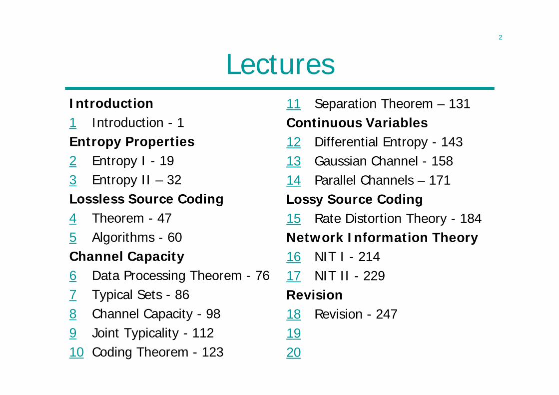
LecturesIntroduction1 Introduction - 1Entropy Properties2 Entropy I - 193 Entropy II – 32Lossless Source Coding4 Theorem - 475 Algorithms - 60Channel Capacity6 Data Processing Theorem - 767 Typical Sets - 868 Channel Capacity - 989 Joint Typicality - 112 10 Coding Theorem - 123
11 Separation Theorem – 131Continuous Variables12 Differential Entropy - 14313 Gaussian Channel - 15814 Parallel Channels – 171Lossy Source Coding15 Rate Distortion Theory - 184 Network Information Theory16 NIT I - 21417 NIT II - 229Revision18 Revision - 2471920
3
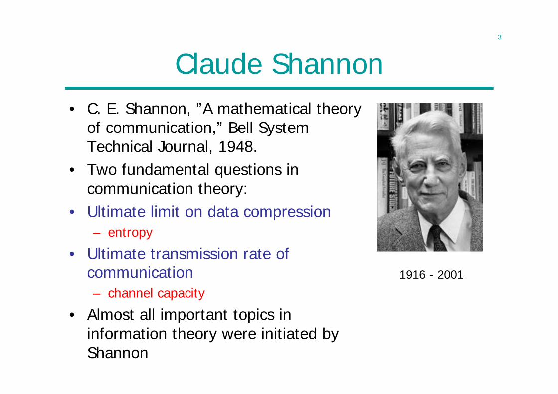
Claude Shannon• C. E. Shannon, ”A mathematical theory
of communication,” Bell System Technical Journal, 1948.
• Two fundamental questions in communication theory:
• Ultimate limit on data compression– entropy
• Ultimate transmission rate of communication– channel capacity
• Almost all important topics in information theory were initiated by Shannon
1916 - 2001
4
Origin of Information Theory
• Common wisdom in 1940s:– It is impossible to send information error-free at a positive rate– Error control by using retransmission: rate 0 if error-free
• Still in use today– ARQ (automatic repeat request) in TCP/IP computer networking
• Shannon showed reliable communication is possible for all rates below channel capacity
• As long as source entropy is less than channel capacity, asymptotically error-free communication can be achieved
• And anything can be represented in bits– Rise of digital information technology

5
Relationship to Other Fields
6
Course Objectives
• In this course we will (focus on communication theory):– Define what we mean by information.– Show how we can compress the information in a
source to its theoretically minimum value and show the tradeoff between data compression and distortion.
– Prove the channel coding theorem and derive the information capacity of different channels.
– Generalize from point-to-point to network information theory.
7
Relevance to Practice
• Information theory suggests means of achieving ultimate limits of communication– Unfortunately, these theoretically optimum schemes
are computationally impractical– So some say “little info, much theory” (wrong)
• Today, information theory offers useful guidelines to design of communication systems– Turbo code (approaches channel capacity)– CDMA (has a higher capacity than FDMA/TDMA)– Channel-coding approach to source coding (duality)– Network coding (goes beyond routing)
8
Books/ReadingBook of the course:• Elements of Information Theory by T M Cover & J A Thomas, Wiley,
£39 for 2nd ed. 2006, or £14 for 1st ed. 1991 (Amazon)
Free references• Information Theory and Network Coding by R. W. Yeung, Springer
http://iest2.ie.cuhk.edu.hk/~whyeung/book2/
• Information Theory, Inference, and Learning Algorithms by D MacKay, Cambridge University Press http://www.inference.phy.cam.ac.uk/mackay/itila/
• Lecture Notes on Network Information Theory by A. E. Gamal and Y.-H. Kim, (Book is published by Cambridge University Press)http://arxiv.org/abs/1001.3404
• C. E. Shannon, ”A mathematical theory of communication,” Bell System Technical Journal, Vol. 27, pp. 379–423, 623–656, July, October, 1948.
9
Other Information
• Course webpage:http://www.commsp.ee.ic.ac.uk/~cling
• Assessment: Exam only – no coursework.• Students are encouraged to do the problems in
problem sheets.• Background knowledge
– Mathematics – Elementary probability
• Needs intellectual maturity– Doing problems is not enough; spend some time
thinking
10
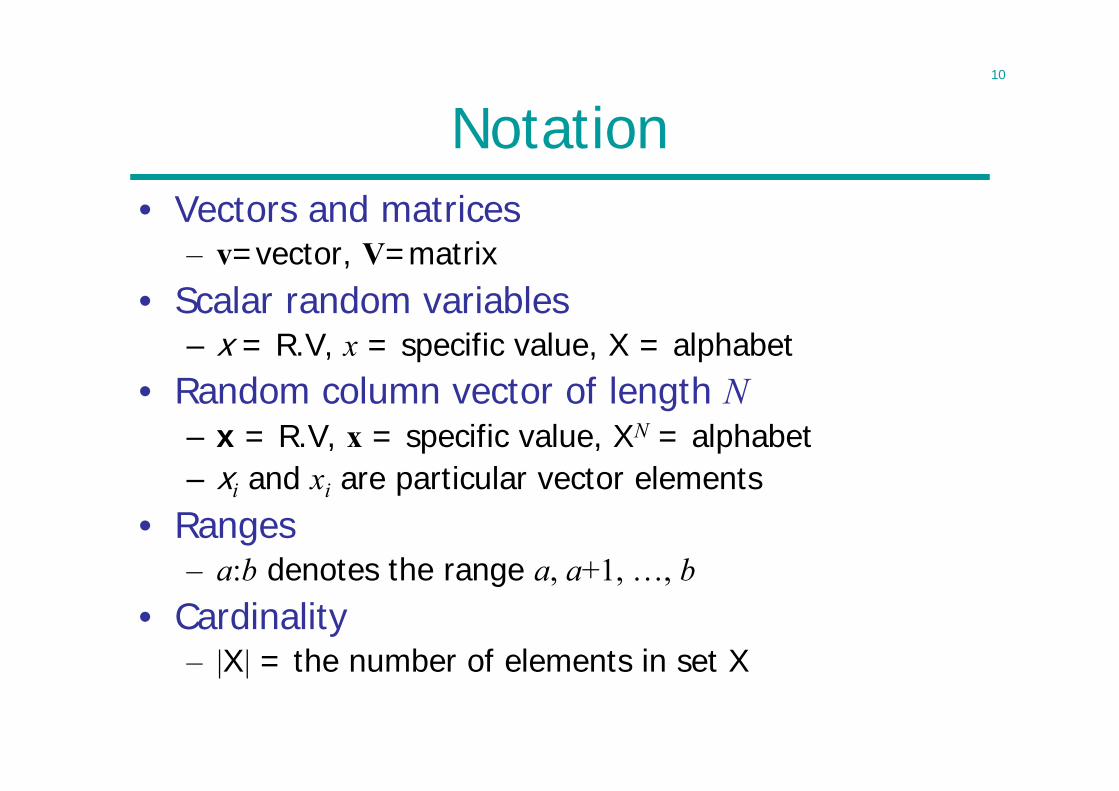
Notation• Vectors and matrices
– v=vector, V=matrix• Scalar random variables
– x = R.V, x = specific value, X = alphabet• Random column vector of length N
– x = R.V, x = specific value, XN = alphabet– xi and xi are particular vector elements
• Ranges– a:b denotes the range a, a+1, …, b
• Cardinality– |X| = the number of elements in set X
11
Discrete Random Variables
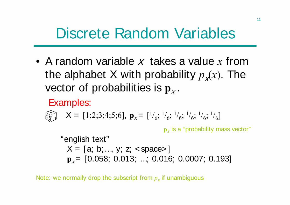
• A random variable x takes a value x from the alphabet X with probability px(x). The vector of probabilities is px .Examples:
X = [1;2;3;4;5;6], px = [1/6; 1/6; 1/6; 1/6; 1/6; 1/6]
“english text”X = [a; b;…, y; z; <space>]px = [0.058; 0.013; …; 0.016; 0.0007; 0.193]
Note: we normally drop the subscript from px if unambiguous
pX is a “probability mass vector”
12
Expected Values
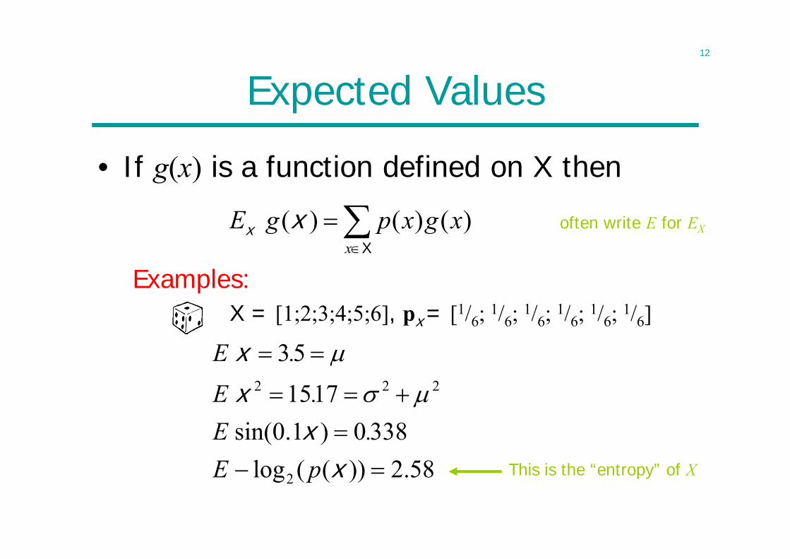
• If g(x) is a function defined on X then
( ) ( ) ( )x
E g p x g x
x xX
Examples:X = [1;2;3;4;5;6], px = [1/6; 1/6; 1/6; 1/6; 1/6; 1/6]
58.2))((log3380)1.0sin(
171553
2
222
xx
xx
pE.E
.E.E
This is the “entropy” of X
often write E for EX
13
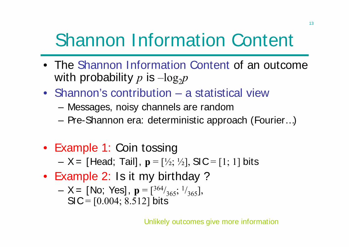
Shannon Information Content• The Shannon Information Content of an outcome
with probability p is –log2p• Shannon’s contribution – a statistical view
– Messages, noisy channels are random– Pre-Shannon era: deterministic approach (Fourier…)
• Example 1: Coin tossing– X = [Head; Tail], p = [½; ½], SIC = [1; 1] bits
• Example 2: Is it my birthday ?– X = [No; Yes], p = [364/365; 1/365],
SIC = [0.004; 8.512] bits
Unlikely outcomes give more information
14
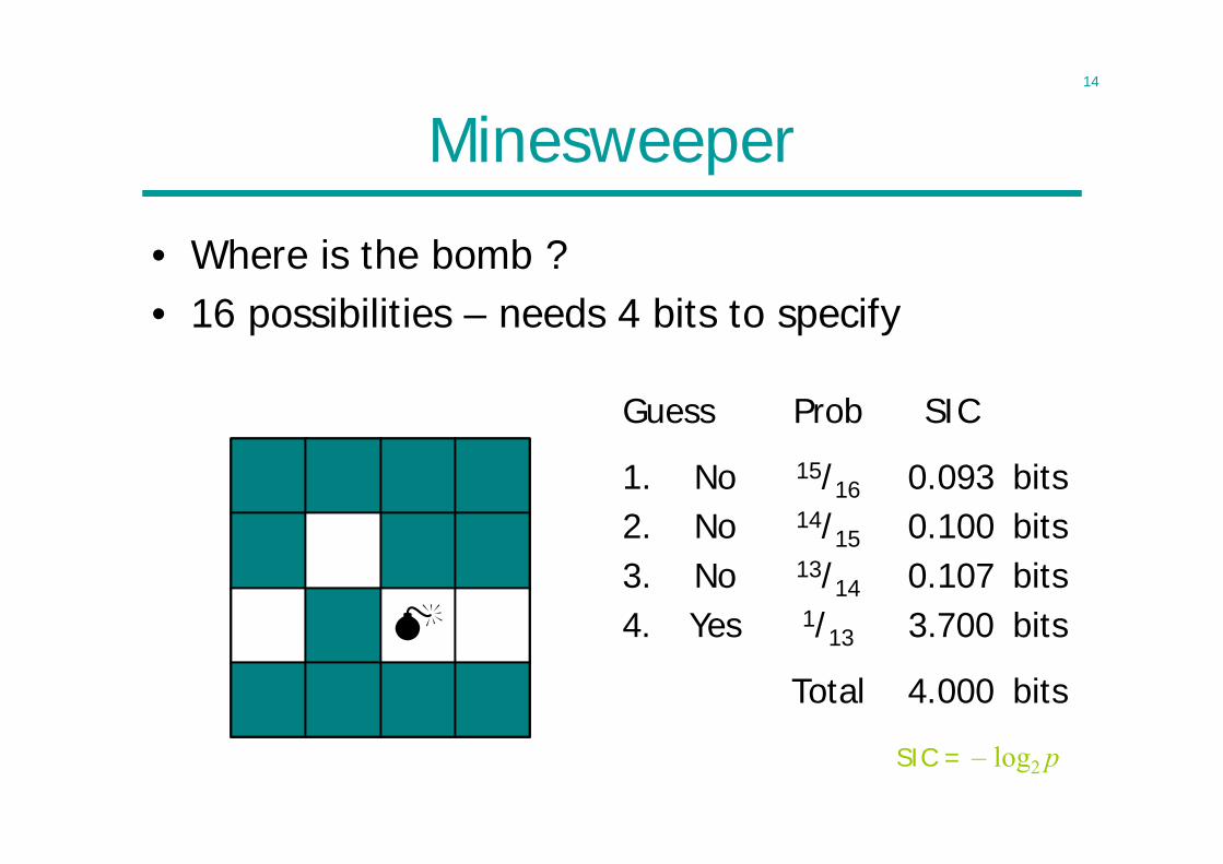
Minesweeper
• Where is the bomb ?• 16 possibilities – needs 4 bits to specify
Guess Prob SIC
Total 4.000 bits
1. No 15/16 0.093 bits2. No 14/15 0.100 bits3. No 13/14 0.107 bits
4. Yes 1/13 3.700 bits
SIC = – log2 p
15
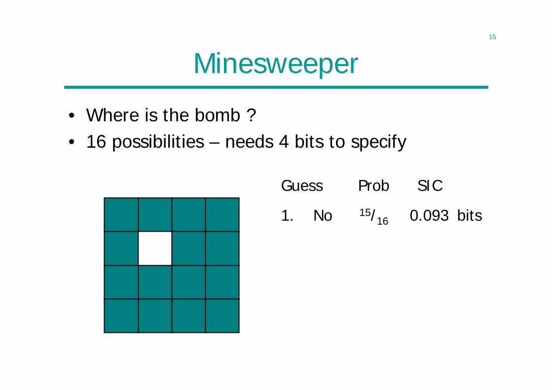
Minesweeper
• Where is the bomb ?• 16 possibilities – needs 4 bits to specify
Guess Prob SIC
1. No 15/16 0.093 bits
16
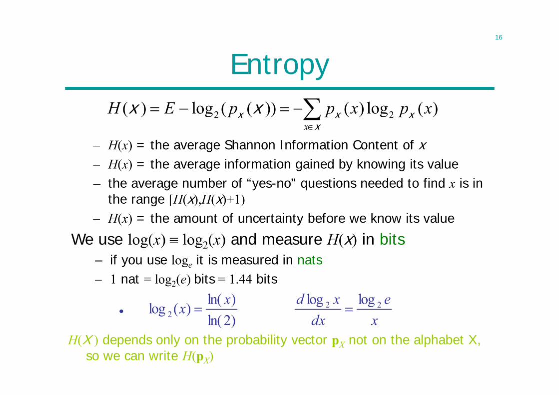
Entropy
– H(x) = the average Shannon Information Content of x– H(x) = the average information gained by knowing its value– the average number of “yes-no” questions needed to find x is in
the range [H(x),H(x)+1)– H(x) = the amount of uncertainty before we know its value
2 2( ) log ( ( )) ( ) log ( )x
H E p p x p x
x x xx
x x
H(X ) depends only on the probability vector pX not on the alphabet X, so we can write H(pX)
We use log(x) log2(x) and measure H(x) in bits– if you use loge it is measured in nats– 1 nat = log2(e) bits = 1.44 bits
• xe
dxxdxx 22
2loglog
)2ln()ln()(log
17
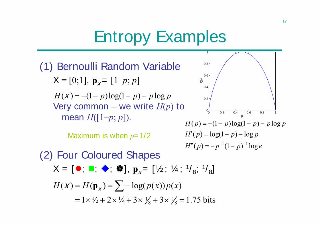
Entropy Examples
(1) Bernoulli Random VariableX = [0;1], px = [1–p; p]
Very common – we write H(p) tomean H([1–p; p]).
(2) Four Coloured ShapesX = [; ; ; ], px = [½; ¼; 1/8; 1/8]
ppppH log)1log()1()( x
bits75.133¼2½1)())(log()()(
81
81
xpxpHH xx p
0 0.2 0.4 0.6 0.8 10
0.2
0.4
0.6
0.8
1
p
H(p
)
Maximum is when p=1/2epppH
pppHpppppH
log)1()(log)1log()(
log)1log()1()(
11
18
Comments on Entropy• Entropy plays a central role in information
theory• Origin in thermodynamics
– S = k ln, k: Boltzman’s constant, : number of microstates
– The second law: entropy of an isolated system is non-decreasing
• Shannon entropy– Agrees with intuition: additive, monotonic, continuous– Logarithmic measure could be derived from an
axiomatic approach (Shannon 1948)
19
Lecture 2
• Joint and Conditional Entropy– Chain rule
• Mutual Information– If x and y are correlated, their mutual information is
the average information that y gives about x• E.g. Communication Channel: x transmitted but y received• It is the amount of information transmitted through the
channel
• Jensen’s Inequality
20
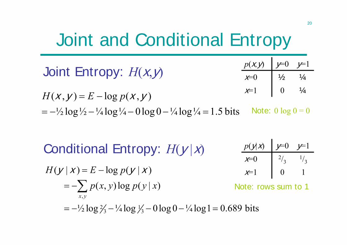
Joint and Conditional Entropy
Joint Entropy: H(x,y)p(x,y) y=0 y=1x=0 ½ ¼
x=1 0 ¼
bits 5.1¼log¼0log0¼log¼½log½),(log),(
yxyx pEH
Conditional Entropy: H(y |x)
,
2 13 3
( | ) log ( | )( , ) log ( | )
½ log ¼ log 0log 0 ¼ log1 0.689 bitsx y
H E pp x y p y x
y x y x
Note: 0 log 0 = 0
p(y|x) y=0 y=1x=0 2/3
1/3
x=1 0 1
Note: rows sum to 1
21
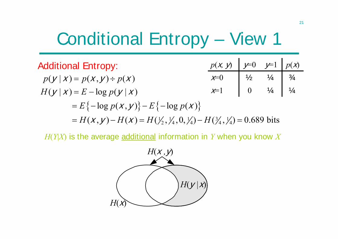
Conditional Entropy – View 1p(x, y) y=0 y=1 p(x)x=0 ½ ¼ ¾
x=1 0 ¼ ¼
Additional Entropy:
31 1 1 1
2 4 4 4 4
( | ) ( , ) ( )( | ) log ( | )
log ( , ) log ( )( , ) ( ) ( , ,0, ) ( , ) 0.689 bits
p p pH E p
E p E pH H H H
y x x y xy x y x
x y xx y x
H(Y|X) is the average additional information in Y when you know X
H(y |x)
H(x ,y)
H(x)
22
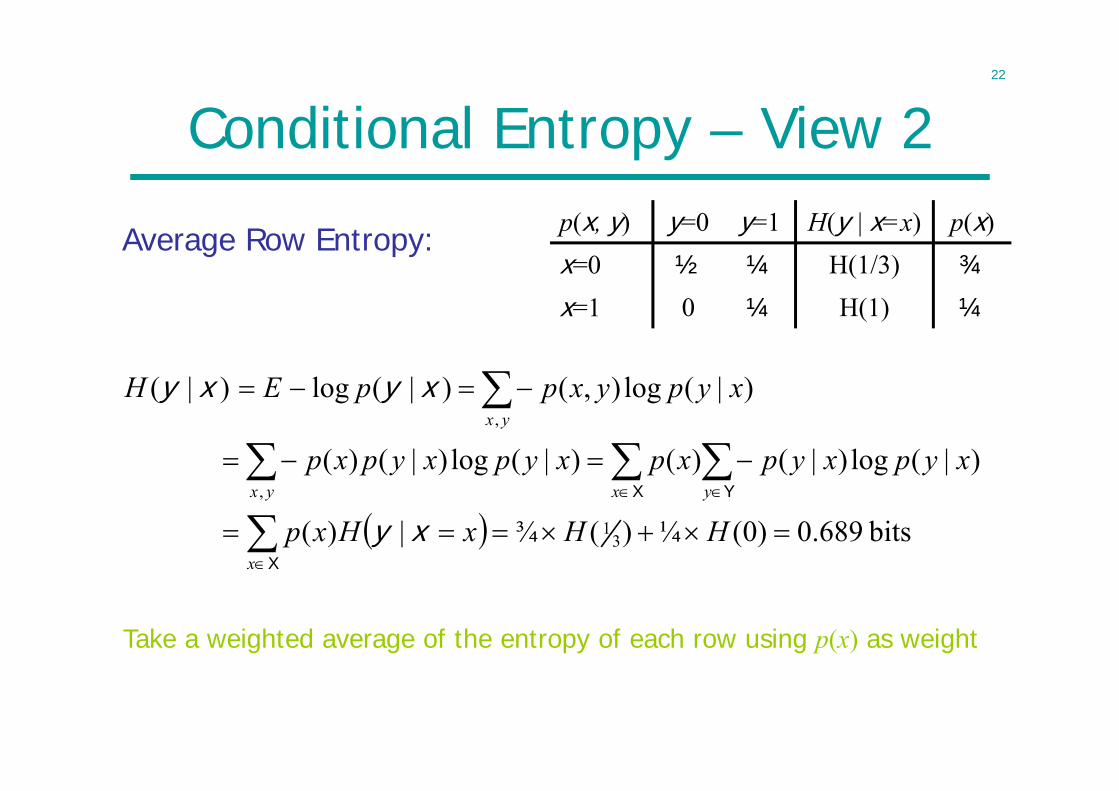
Conditional Entropy – View 2
Average Row Entropy:
bits 689.0)0(¼)(¾|)(
)|(log)|()()|(log)|()(
)|(log),()|(log)|(
31
,
,
HHxHxp
xypxypxpxypxypxp
xypyxppEH
x
x yyx
yx
X
X Y
xy
xyxy
p(x, y) y=0 y=1 H(y | x=x) p(x)x=0 ½ ¼ H(1/3) ¾
x=1 0 ¼ H(1) ¼
Take a weighted average of the entropy of each row using p(x) as weight
23
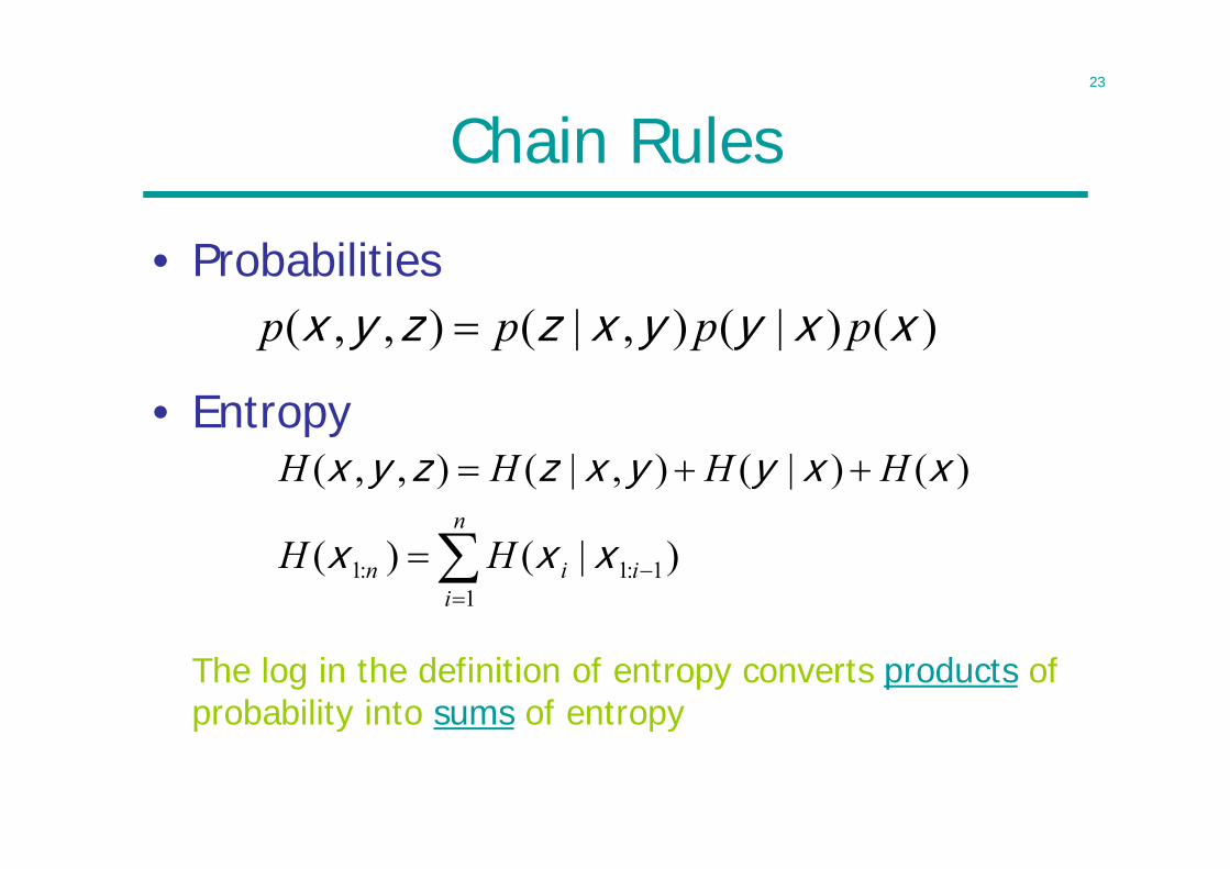
Chain Rules
• Probabilities
• Entropy
The log in the definition of entropy converts products of probability into sums of entropy
)()|(),|(),,( xxyyxzzyx pppp
n
iiin HH
HHHH
11:1:1 )|()(
)()|(),|(),,(
xxx
xxyyxzzyx
24
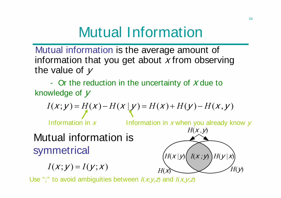
Mutual InformationMutual information is the average amount of information that you get about x from observing the value of y
- Or the reduction in the uncertainty of x due to knowledge of y
);();( xyyx II
),()()()|()();( yxyxyxxyx HHHHHI
Use “;” to avoid ambiguities between I(x;y,z) and I(x,y;z)
Information in x Information in x when you already know y
Mutual information is symmetrical H(x |y) H(y |x)
H(x ,y)
H(x) H(y)
I(x ;y)
25
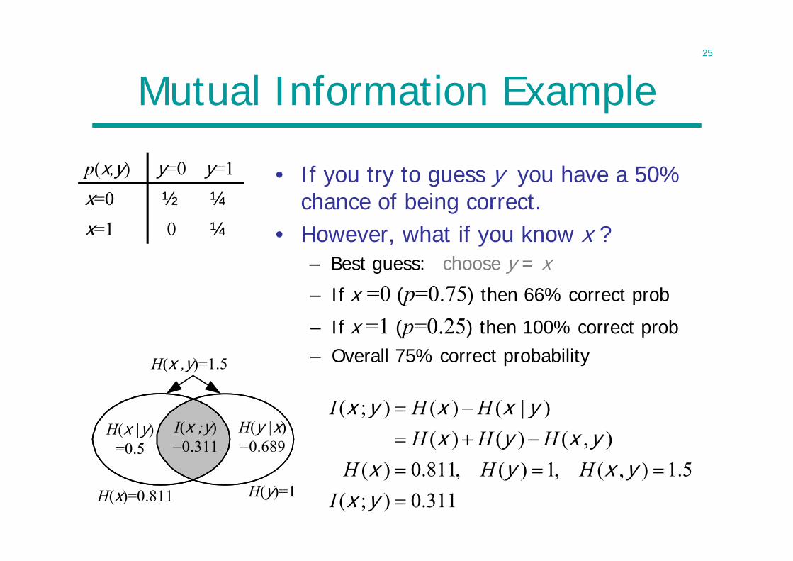
Mutual Information Example
• If you try to guess y you have a 50% chance of being correct.
• However, what if you know x ?– Best guess:
H(x |y)=0.5
H(y |x)=0.689
H(x ,y)=1.5
H(x)=0.811 H(y)=1
I(x ;y)=0.311
p(x,y) y=0 y=1x=0 ½ ¼
x=1 0 ¼
311.0);(5.1),(,1)(,811.0)(
),()()()|()();(
yxyxyx
yxyxyxxyx
IHHH
HHHHHI
choose y = x
– If x =0 (p=0.75) then 66% correct prob
– If x =1 (p=0.25) then 100% correct prob– Overall 75% correct probability
26
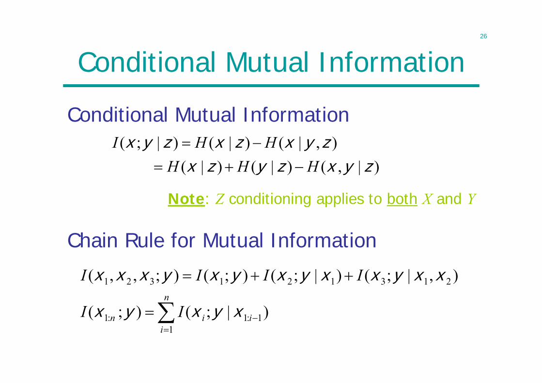
Conditional Mutual Information
Conditional Mutual Information
Note: Z conditioning applies to both X and Y
)|,()|()|(),|()|()|;(
zyxzyzxzyxzxzyx
HHHHHI
n
iiin II
IIII
11:1:1
213121321
)|;();(
),|;()|;();();,,(
xyxyx
xxyxxyxyxyxxx
Chain Rule for Mutual Information
27
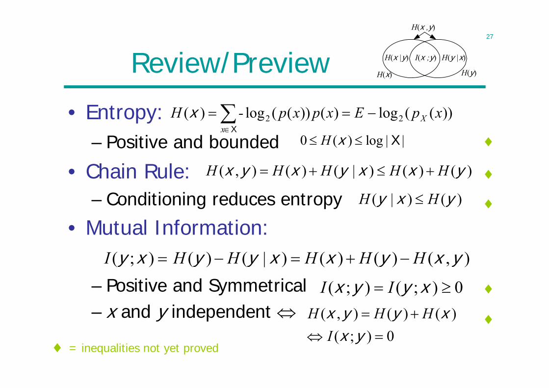
Review/Preview
• Entropy:– Positive and bounded
))((log)())((log)( 22 xpExpxp-H Xx
X
x
0 ( ) log | |H x X
)()()|()(),( yxxyxyx HHHHH
0);()()(),(
yxxyyx
IHHH
),()()()|()();( yxyxxyyxy HHHHHI
0);();( xyyx II
)()|( yxy HH
= inequalities not yet proved
H(x |y) H(y |x)
H(x ,y)
H(x) H(y)
I(x ;y)
• Chain Rule:– Conditioning reduces entropy
• Mutual Information:
– Positive and Symmetrical– x and y independent
28
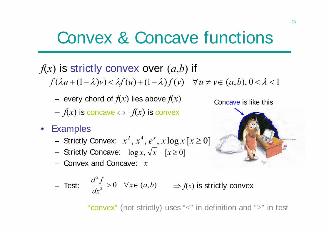
Convex & Concave functions
f(x) is strictly convex over (a,b) if
– every chord of f(x) lies above f(x)– f(x) is concave –f(x) is convex
Concave is like this
10),,()()1()())1(( bavuvfufvuf
),(02
2
baxdx
fd
]0[ log,,, 42 xxxexx x
]0[,log xxxx
• Examples– Strictly Convex: – Strictly Concave: – Convex and Concave:
– Test: f(x) is strictly convex
“convex” (not strictly) uses “” in definition and “” in test
29
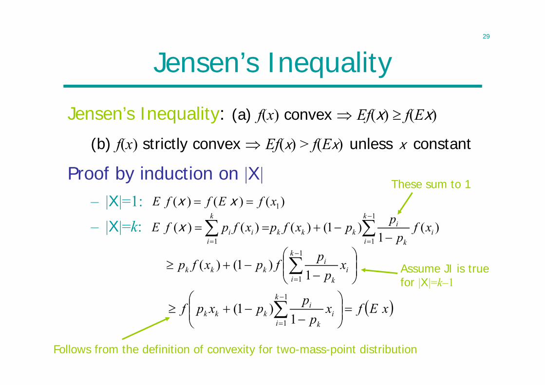
Jensen’s Inequality
Jensen’s Inequality: (a) f(x) convex Ef(x) f(Ex)
(b) f(x) strictly convex Ef(x) > f(Ex) unless x constant
Proof by induction on |X|– |X|=1: )()()( 1xfEffE xx
1
11
)(1
)1()()()(k
ii
k
ikkk
k
iii xf
pppxfpxfpfE x
Assume JI is true for |X|=k–1
These sum to 1
Follows from the definition of convexity for two-mass-point distribution
1
1 1)1()(
k
ii
k
ikkk x
ppfpxfp
xEfxp
ppxpfk
ii
k
ikkk
1
1 1)1(
– |X|=k:
30
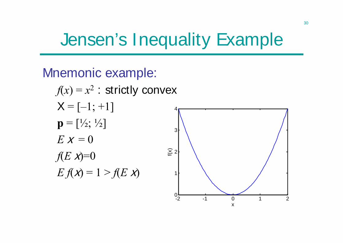
Jensen’s Inequality Example
Mnemonic example:f(x) = x2 : strictly convexX = [–1; +1]p = [½; ½]E x = 0f(E x)=0E f(x) = 1 > f(E x)
-2 -1 0 1 20
1
2
3
4
x
f(x)
31
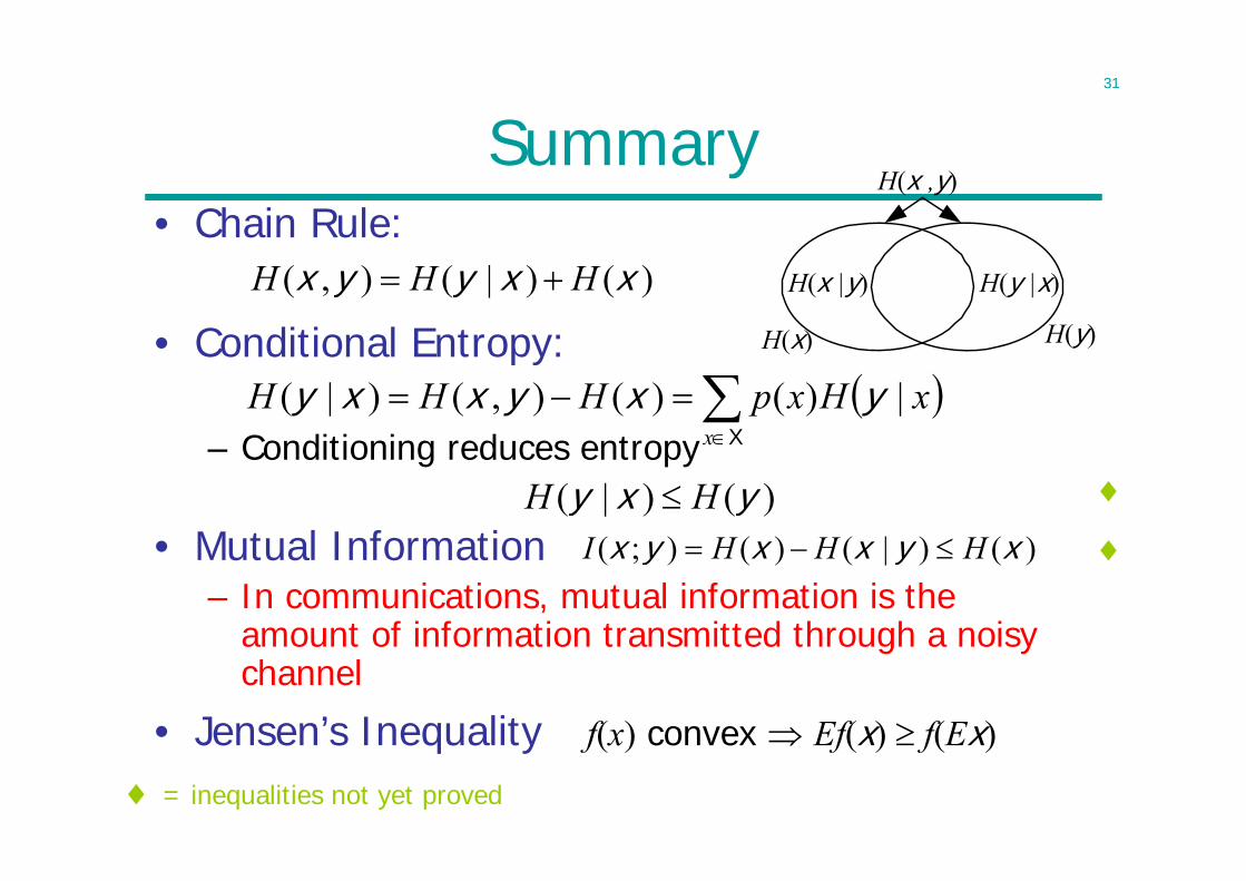
Summary• Chain Rule:
• Conditional Entropy:
– Conditioning reduces entropy
• Mutual Information– In communications, mutual information is the
amount of information transmitted through a noisy channel
• Jensen’s Inequality f(x) convex Ef(x) f(Ex)
)()|(),( xxyyx HHH
)()|( yxy HH
= inequalities not yet proved
Xx
xHxpHHH |)()(),()|( yxyxxy
H(x |y) H(y |x)
H(x ,y)
H(x) H(y)
)()|()();( xyxxyx HHHI
32
Lecture 3
• Relative Entropy– A measure of how different two probability mass
vectors are• Information Inequality and its consequences
– Relative Entropy is always positive• Mutual information is positive• Uniform bound• Conditioning and correlation reduce entropy
• Stochastic Processes– Entropy Rate– Markov Processes
33
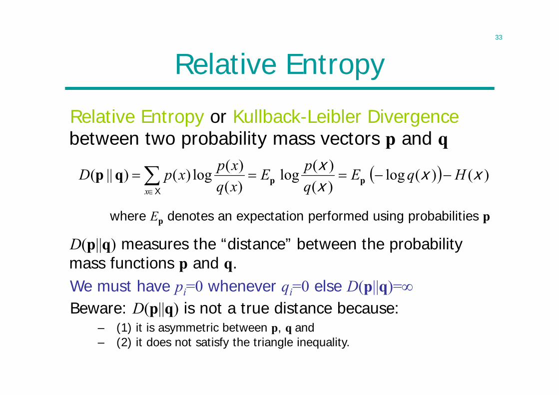
Relative Entropy
Relative Entropy or Kullback-Leibler Divergencebetween two probability mass vectors p and q
)()(log)()(log
)()(log)()||( xx
xx HqE
qpE
xqxpxpD
x
ppqp
X
where Ep denotes an expectation performed using probabilities p
D(p||q) measures the “distance” between the probability mass functions p and q. We must have pi=0 whenever qi=0 else D(p||q)=Beware: D(p||q) is not a true distance because:
– (1) it is asymmetric between p, q and– (2) it does not satisfy the triangle inequality.
34
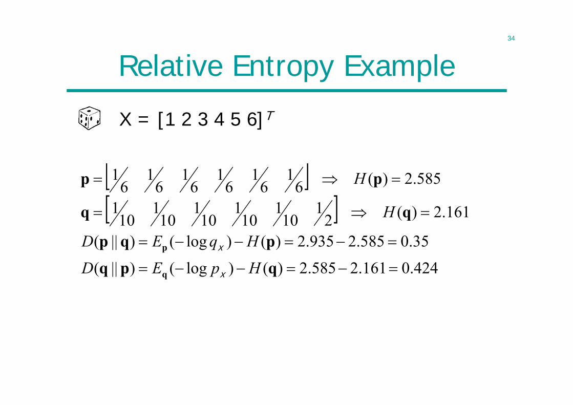
Relative Entropy Example
X = [1 2 3 4 5 6]T
424.0161.2585.2)()log()||(
35.0585.2935.2)()log()||(
161.2)(21
101
101
101
101
101
585.2)(61
61
61
61
61
61
qpq
pqp
pp
q
p
HpED
HqED
H
H
x
x
35
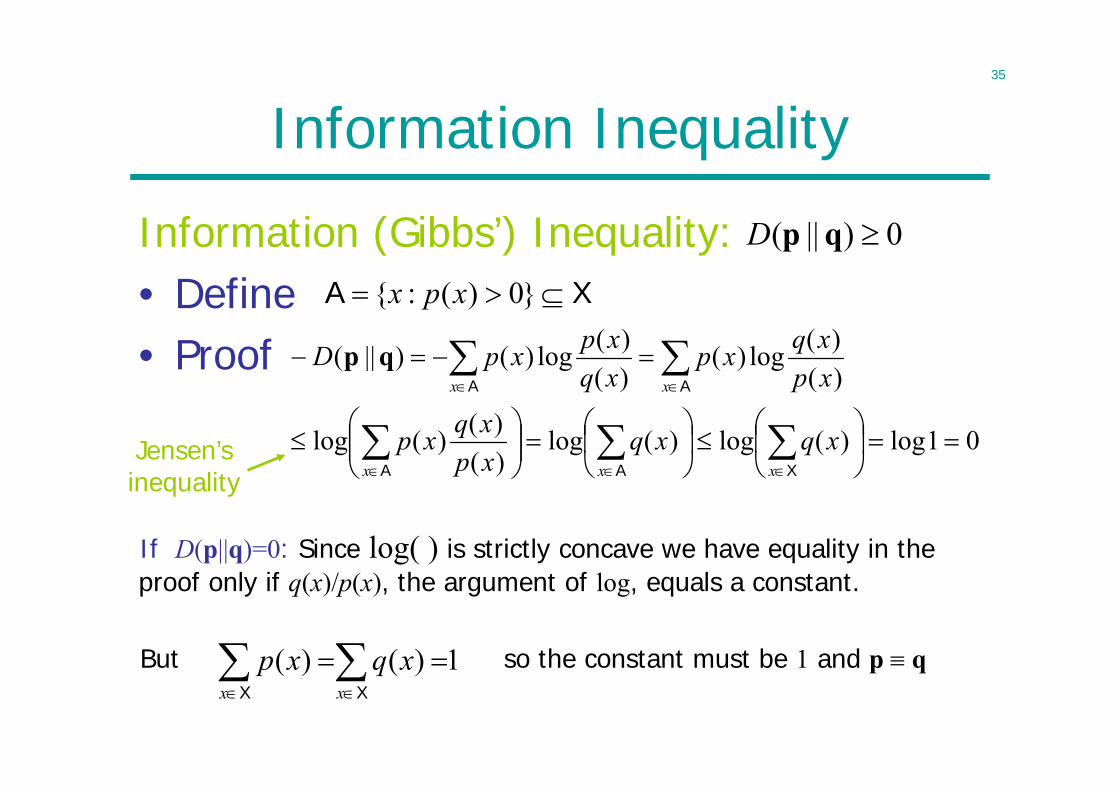
Information Inequality
Information (Gibbs’) Inequality:• Define • Proof
0)||( qpD
XA }0)(:{ xpx
01log)(log)(log)()()(log
)()(log)(
)()(log)()||(
XAA
AA
xxx
xx
xqxqxpxqxp
xpxqxp
xqxpxpD qp
If D(p||q)=0: Since log( ) is strictly concave we have equality in the proof only if q(x)/p(x), the argument of log, equals a constant.
But so the constant must be 1 and p q1)()(
XX xx
xqxp
Jensen’s inequality
36
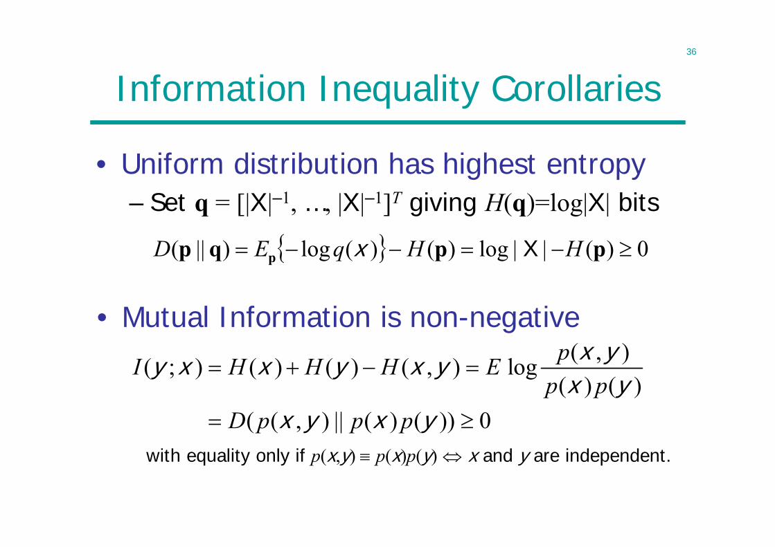
Information Inequality Corollaries
• Uniform distribution has highest entropy– Set q = [|X|–1, …, |X|–1]T giving H(q)=log|X| bits
0)(||log)()(log)||( ppqp p HHqED Xx
• Mutual Information is non-negative( , )( ; ) ( ) ( ) ( , ) log
( ) ( )( ( , ) || ( ) ( )) 0
pI H H H Ep p
D p p p
x yy x x y x yx y
x y x ywith equality only if p(x,y) p(x)p(y) x and y are independent.
37
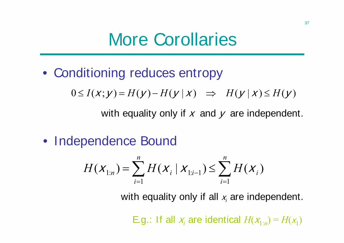
More Corollaries
• Conditioning reduces entropy)()|()|()();(0 yxyxyyyx HHHHI
• Independence Bound
n
ii
n
iiin HHH
111:1:1 )()|()( xxxx
with equality only if x and y are independent.
with equality only if all xi are independent.
E.g.: If all xi are identical H(x1:n) = H(x1)
38
Conditional Independence Bound
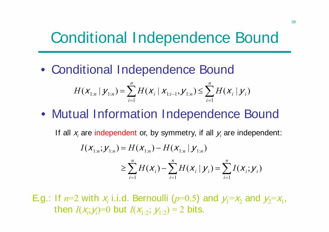
• Conditional Independence Bound
• Mutual Information Independence Bound
n
iii
n
iniinn HHH
11:11:1:1:1 )|(),|()|( yxyxxyx
If all xi are independent or, by symmetry, if all yi are independent:
n
iii
n
iii
n
ii
nnnnn
IHH
HHI
111
:1:1:1:1:1
);()|()(
)|()();(
yxyxx
yxxyx
E.g.: If n=2 with xi i.i.d. Bernoulli (p=0.5) and y1=x2 and y2=x1, then I(xi;yi)=0 but I(x1:2; y1:2) = 2 bits.
39
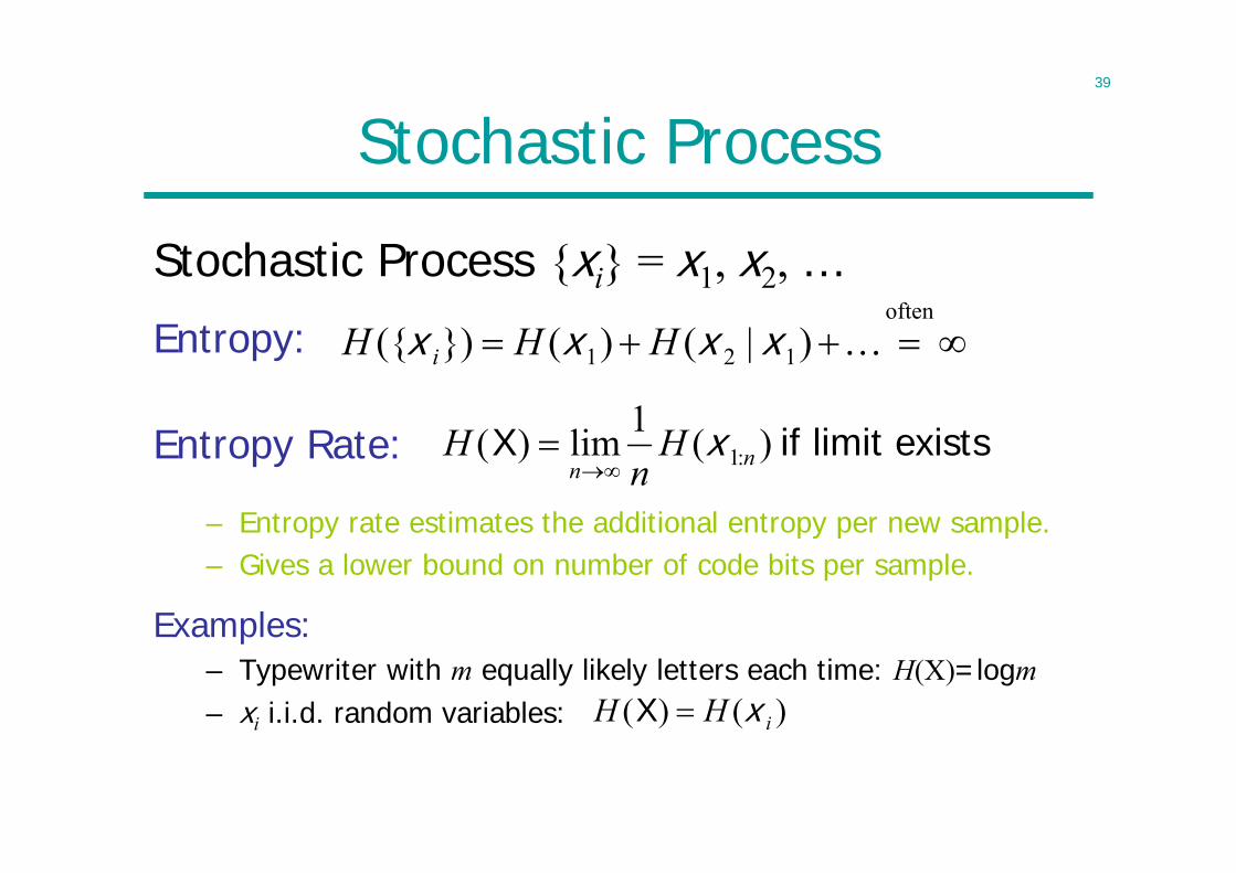
Stochastic Process
Stochastic Process {xi} = x1, x2, …Entropy:
Entropy Rate:
– Entropy rate estimates the additional entropy per new sample.– Gives a lower bound on number of code bits per sample.
Examples:– Typewriter with m equally likely letters each time: H(X)=logm– xi i.i.d. random variables:
often
121 )|()(})({ xxxx HHH i
existslimit if )(1lim)( :1 nnH
nH x
X
)()( iHH xX

40
Stationary Process
Stochastic Process {xi} is stationary iff
X innknn ankapap ,,)()( :1):1(:1:1 xx
If {xi} is stationary then H(X) exists and
)|(lim)(1lim)( 1:1:1 nnnnn
HHn
H xxxX
Proof: )|()|()|(0 2:11
)b(
1:2
)a(
1:1 nnnnnn HHH xxxxxx
Hence H(xn|x1:n-1) is positive, decreasing tends to a limit, say b
(a) conditioning reduces entropy, (b) stationarity
)()|(1)(1)|(1
1:1:11:1 XHbHn
Hn
bHn
kkknkk
xxxxx
Hence
41
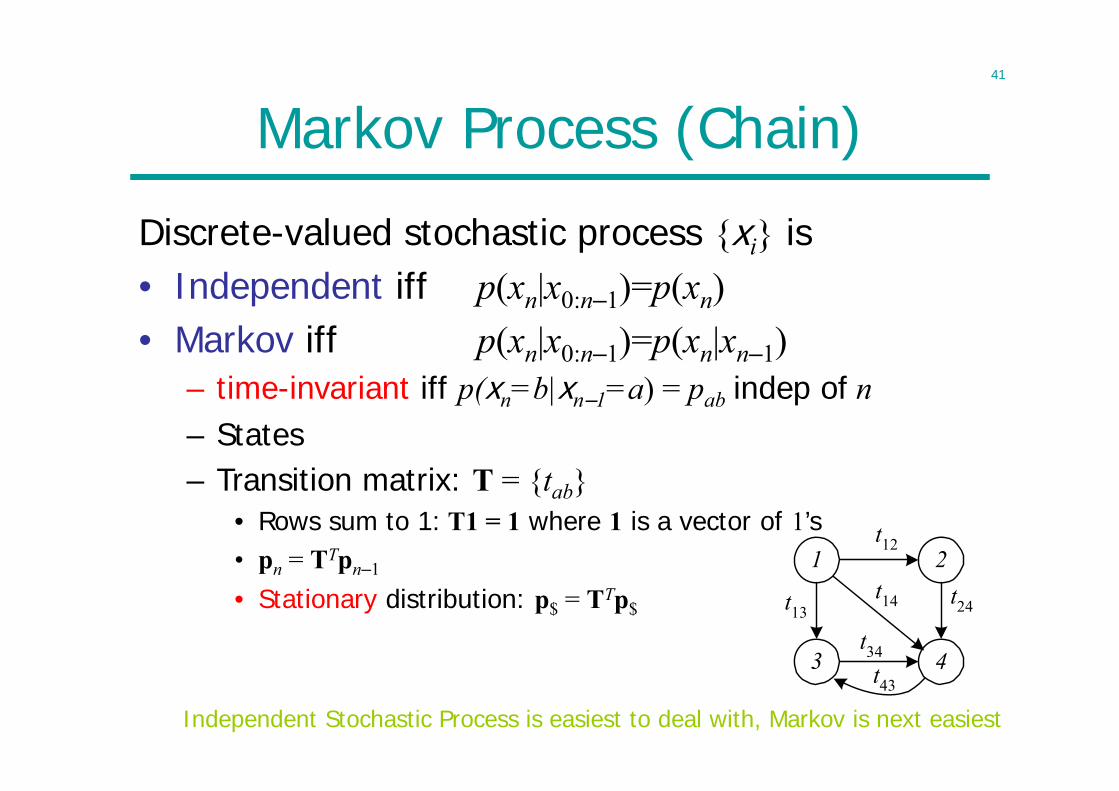
Markov Process (Chain)
Discrete-valued stochastic process {xi} is• Independent iff p(xn|x0:n–1)=p(xn)• Markov iff p(xn|x0:n–1)=p(xn|xn–1)
1
3 4
2t12
t13t24
t14
t34t43
Independent Stochastic Process is easiest to deal with, Markov is next easiest
– time-invariant iff p(xn=b|xn–1=a) = pab indep of n– States– Transition matrix: T = {tab}
• Rows sum to 1: T1 = 1 where 1 is a vector of 1’s• pn = TTpn–1
• Stationary distribution: p$ = TTp$
42
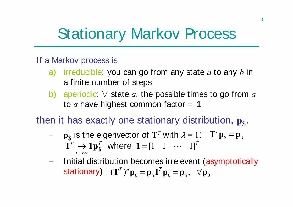
then it has exactly one stationary distribution, p$.– p$ is the eigenvector of TT with = 1:
– Initial distribution becomes irrelevant (asymptotically stationary)
Stationary Markov Process
If a Markov process isa) irreducible: you can go from any state a to any b in
a finite number of stepsb) aperiodic: state a, the possible times to go from a
to a have highest common factor = 1
$$ ppT T
TT
n
n ]111[$
11pT where
0 $ 0 $ 0( ) ,T n T T p p 1 p p p
43
H(p1)=0, H(p1 | p0)=0H(p2)=1.58496, H(p2 | p1)=1.58496H(p3)=3.10287, H(p3 | p2)=2.54795H(p4)=2.99553, H(p4 | p3)=2.09299H(p5)=3.111, H(p5 | p4)=2.30177H(p6)=3.07129, H(p6 | p5)=2.20683H(p7)=3.09141, H(p7 | p6)=2.24987H(p8)=3.0827, H(p8 | p7)=2.23038
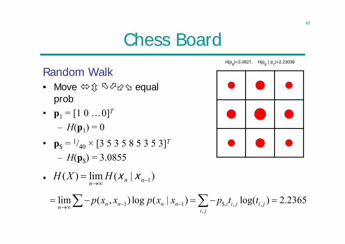
Chess Board
Random Walk• Move equal
prob• p1 = [1 0 … 0]T
– H(p1) = 0
1( ) lim ( | )n nnH X H
x x
• p$ = 1/40 × [3 5 3 5 8 5 3 5 3]T
– H(p$) = 3.0855
•
1 1 $, , ,,
lim ( , ) log ( | ) log( ) 2.2365n n n n i i j i jn i jp x x p x x p t t
44
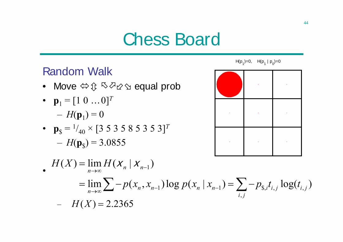
H(p1)=0, H(p1 | p0)=0
Chess Board
Random Walk• Move equal prob• p1 = [1 0 … 0]T
– H(p1) = 0• p$ = 1/40 × [3 5 3 5 8 5 3 5 3]T
– H(p$) = 3.0855
•
–
1
1 1 $, , ,,
( ) lim ( | )
lim ( , ) log ( | ) log( )
n nn
n n n n i i j i jn i j
H X H
p x x p x x p t t
x x
( ) 2.2365H X
45
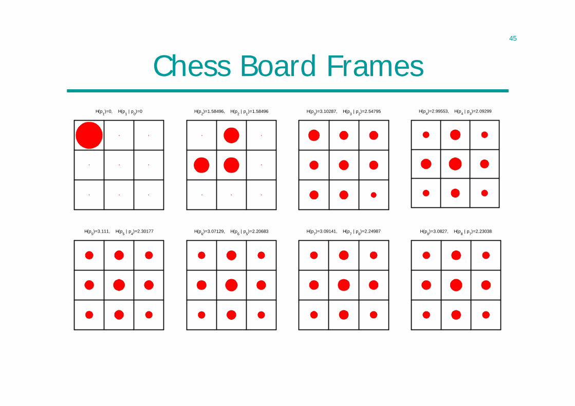
Chess Board FramesH(p1)=0, H(p1 | p0)=0 H(p2)=1.58496, H(p2 | p1)=1.58496 H(p3)=3.10287, H(p3 | p2)=2.54795 H(p4)=2.99553, H(p4 | p3)=2.09299
H(p5)=3.111, H(p5 | p4)=2.30177 H(p6)=3.07129, H(p6 | p5)=2.20683 H(p7)=3.09141, H(p7 | p6)=2.24987 H(p8)=3.0827, H(p8 | p7)=2.23038
46
Summary0
)()(log)||(
xx
qpED pqp
n
iiinn
n
iin HHHH
1:1:1
1:1 )|()|()()( yxyxxx
indep are or if ii
n
iiinn II yxyxyx
1
:1:1 );();(
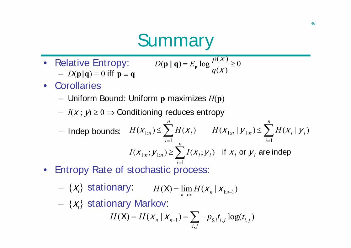
• Relative Entropy:– D(p||q) = 0 iff p q
• Corollaries– Uniform Bound: Uniform p maximizes H(p)
– I(x ; y) 0 Conditioning reduces entropy
– Indep bounds:
• Entropy Rate of stochastic process:
1: 1( ) lim ( | )n nnH H
x xX
1 $, , ,,
( ) ( | ) log( )n n i i j i ji j
H H p t t x xX
– {xi} stationary:
– {xi} stationary Markov:
47
Lecture 4
• Source Coding Theorem– n i.i.d. random variables each with entropy H(X) can
be compressed into more than nH(X) bits as n tends to infinity
• Instantaneous Codes– Symbol-by-symbol coding– Uniquely decodable
• Kraft Inequality– Constraint on the code length
• Optimal Symbol Code lengths– Entropy Bound
48
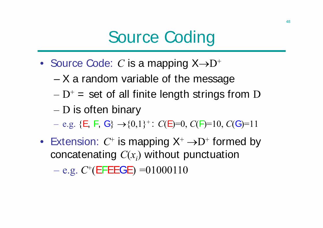
Source Coding• Source Code: C is a mapping XD+
– X a random variable of the message– D+ = set of all finite length strings from D– D is often binary– e.g. {E, F, G} {0,1}+ : C(E)=0, C(F)=10, C(G)=11
• Extension: C+ is mapping X+ D+ formed by concatenating C(xi) without punctuation– e.g. C+(EFEEGE) =01000110
49
Desired Properties
• Non-singular: x1 x2 C(x1) C(x2)– Unambiguous description of a single letter of X
• Uniquely Decodable: C+ is non-singular– The sequence C+(x+) is unambiguous– A stronger condition– Any encoded string has only one possible source
string producing it– However, one may have to examine the entire
encoded string to determine even the first source symbol
– One could use punctuation between two codewords but inefficient
50
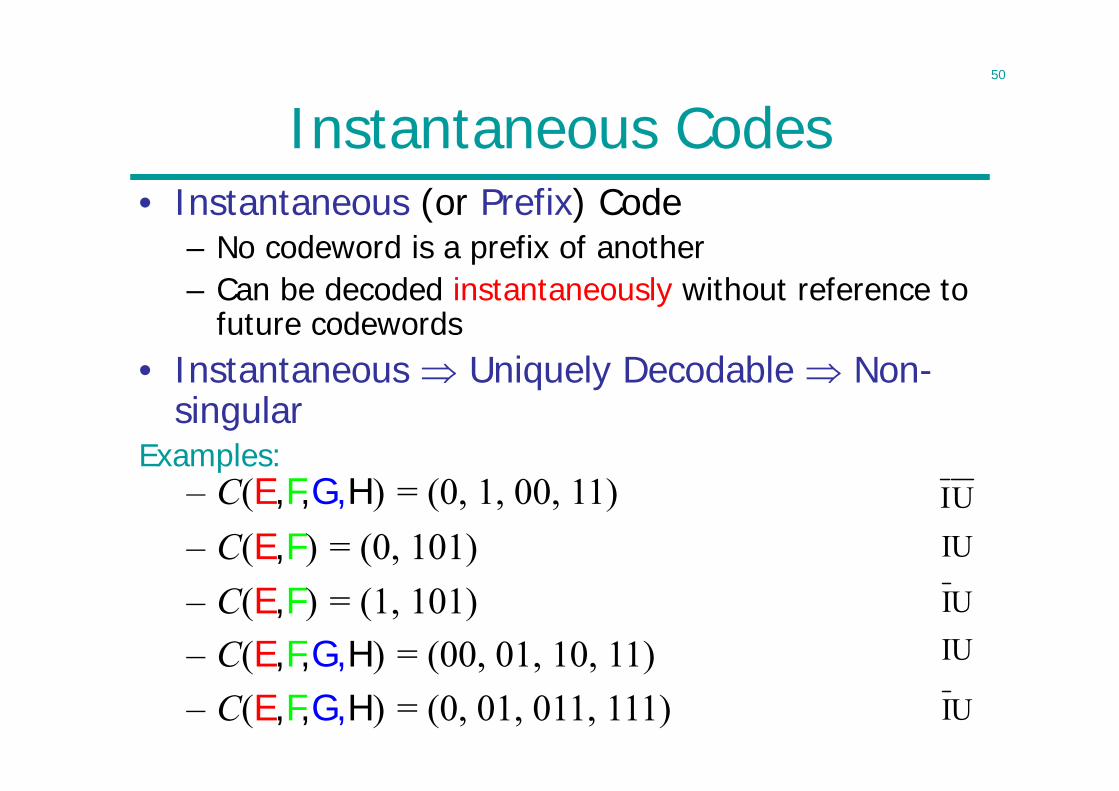
Instantaneous Codes• Instantaneous (or Prefix) Code
– No codeword is a prefix of another– Can be decoded instantaneously without reference to
future codewords• Instantaneous Uniquely Decodable Non-
singularExamples:
IUIU
IUIU
IU
– C(E,F,G,H) = (0, 1, 00, 11)– C(E,F) = (0, 101)– C(E,F) = (1, 101)– C(E,F,G,H) = (00, 01, 10, 11)– C(E,F,G,H) = (0, 01, 011, 111)
51
Code Tree
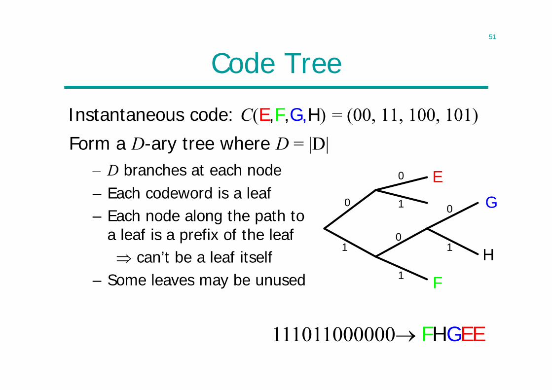
Instantaneous code: C(E,F,G,H) = (00, 11, 100, 101)
1
0
0
0
1
1
E
F
G
H
0
1
– D branches at each node– Each codeword is a leaf– Each node along the path to
a leaf is a prefix of the leaf can’t be a leaf itself
– Some leaves may be unused
111011000000 FHGEE
Form a D-ary tree where D = |D|
52
Kraft Inequality (instantaneous codes)
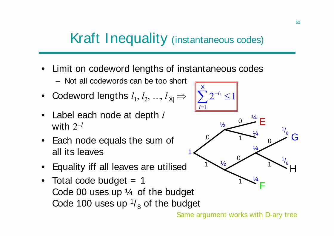
• Limit on codeword lengths of instantaneous codes– Not all codewords can be too short
• Codeword lengths l1, l2, …, l|X|
1
0
0
0
1
1
E
F
G
H
0
1
½
½
¼
¼
¼
¼
1/8
1/81
• Label each node at depth lwith 2–l
• Each node equals the sum of all its leaves
12||
1
X
i
li
• Equality iff all leaves are utilised• Total code budget = 1
Code 00 uses up ¼ of the budgetCode 100 uses up 1/8 of the budget
Same argument works with D-ary tree
53
McMillan Inequality (uniquely decodable codes)
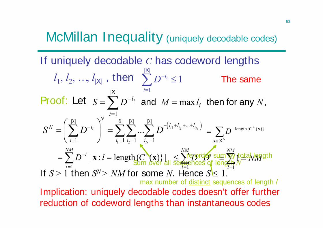
If uniquely decodable C has codeword lengthsl1, l2, …, l|X| , then
Proof: Let
1||
1
X
i
liD
,NlMDS ii
li any for then and max||
1
X
1 2
1 2
| | | | | | | |...
1 1 1 1... i i iNi
N
Nl l llN
i i i iS D D
X X X X
If S > 1 then SN > NM for some N. Hence S 1.
N
CDXx
x)}(length{
Sum over all sequences of length N
NM
l
l ClD1
|)}(length{:| xx
NM
l
ll DD1
NMNM
l
1
1re-order sum by total length
max number of distinct sequences of length lImplication: uniquely decodable codes doesn’t offer further reduction of codeword lengths than instantaneous codes
The same
54
NM
l
l ClD1
|)}(length{:| xx
NM
l
ll DD1
McMillan Inequality (uniquely decodable codes)
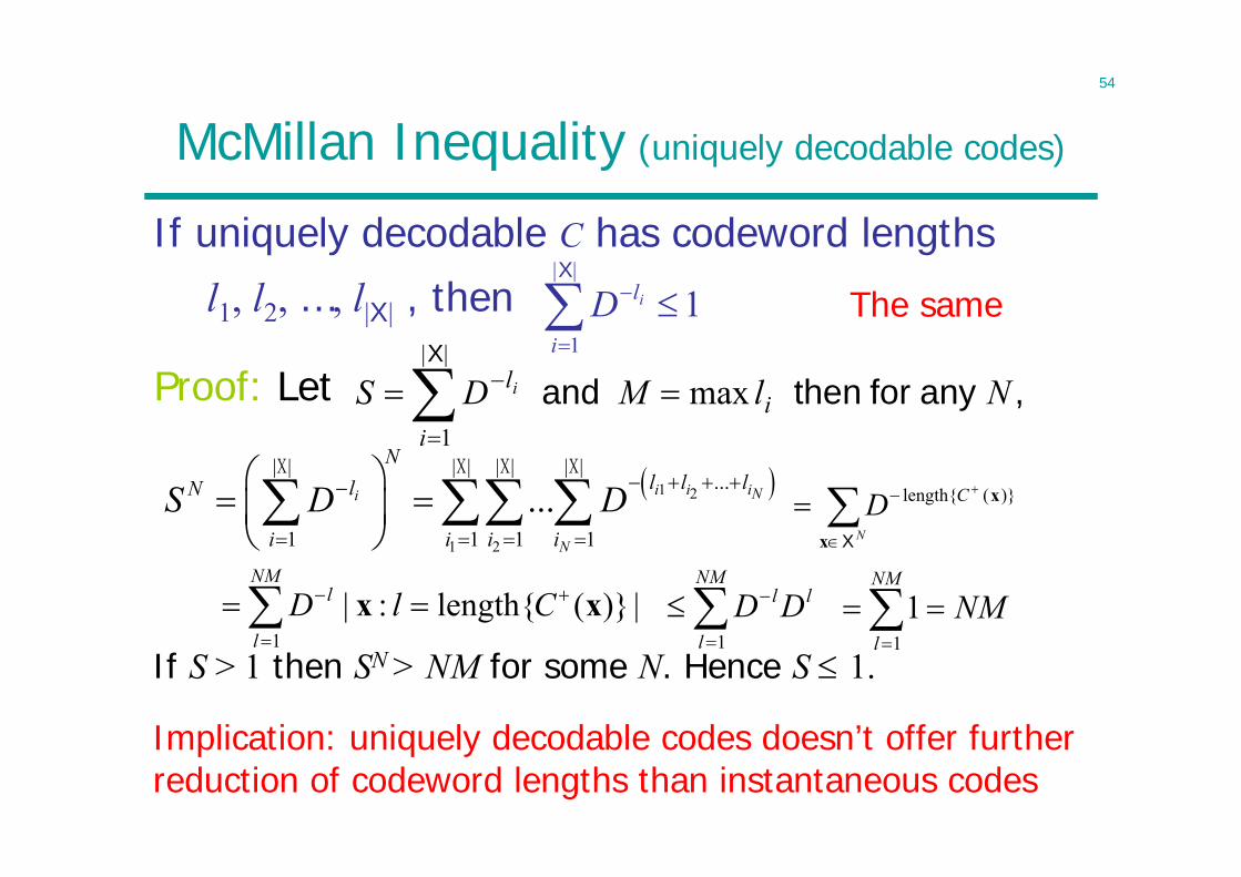
If uniquely decodable C has codeword lengthsl1, l2, …, l|X| , then
Proof: Let
1||
1
X
i
liD
,NlMDS ii
li any for then and max||
1
X
1 2
1 2
| | | | | | | |...
1 1 1 1... i i iNi
N
Nl l llN
i i i iS D D
X X X X
If S > 1 then SN > NM for some N. Hence S 1.
N
CDXx
x)}(length{
NMNM
l
1
1
Implication: uniquely decodable codes doesn’t offer further reduction of codeword lengths than instantaneous codes
The same
55
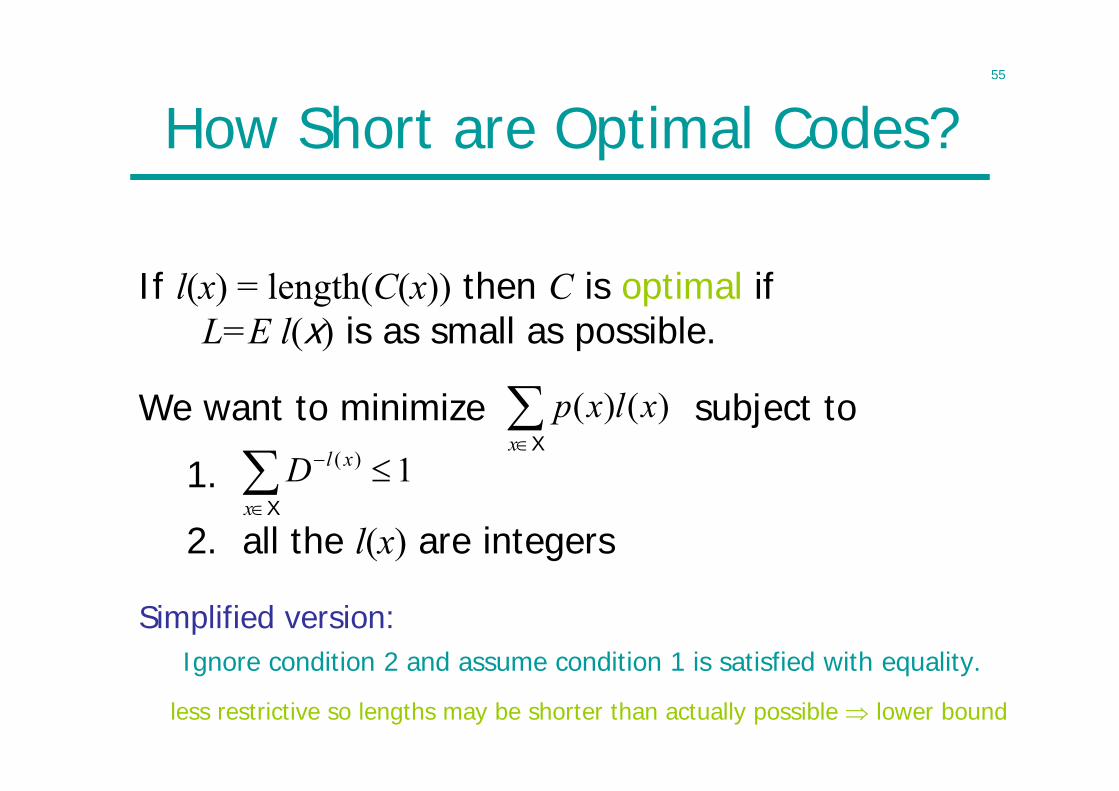
How Short are Optimal Codes?
If l(x) = length(C(x)) then C is optimal ifL=E l(x) is as small as possible.
We want to minimize subject to
1.
2. all the l(x) are integers
Simplified version:Ignore condition 2 and assume condition 1 is satisfied with equality.
Xx
xlxp )()(
1)(
Xx
xlD
less restrictive so lengths may be shorter than actually possible lower bound
56
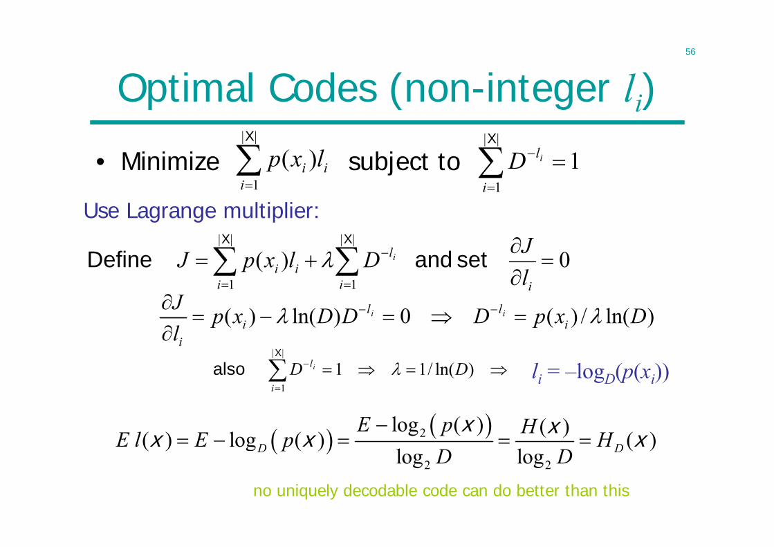
Optimal Codes (non-integer li)
• Minimize subject to
||
1)(
X
iii lxp
0 )(||
1
||
1
ii
l
iii l
JDlxpJ i set and DefineXX
)ln(/)(0)ln()( DxpDDDxplJ
ill
ii
ii
1||
1
X
i
liD
2
2 2
log ( ) ( )( ) log ( ) ( )log logD D
E p HE l E p HD D
x xx x x
no uniquely decodable code can do better than this
li = –logD(p(xi))
)ln(/11||
1
DDi
li X
also
Use Lagrange multiplier:
57
• We can do better by encoding blocks of n symbols
• If entropy rate of xi exists ( xi is stationary process)
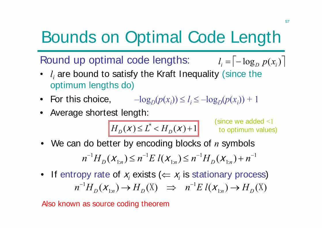
Bounds on Optimal Code LengthRound up optimal code lengths:• li are bound to satisfy the Kraft Inequality (since the
optimum lengths do)
)(log iDi xpl
*( ) ( ) 1D DH L H x x(since we added <1
to optimum values)
• For this choice, –logD(p(xi)) li –logD(p(xi)) + 1• Average shortest length:
1 1 1 11: 1: 1:( ) ( ) ( )D n n D nn H n E l n H n x x x
1 11: 1:( ) ( ) ( ) ( )D n D n Dn H H n E l H x xX X
Also known as source coding theorem
58
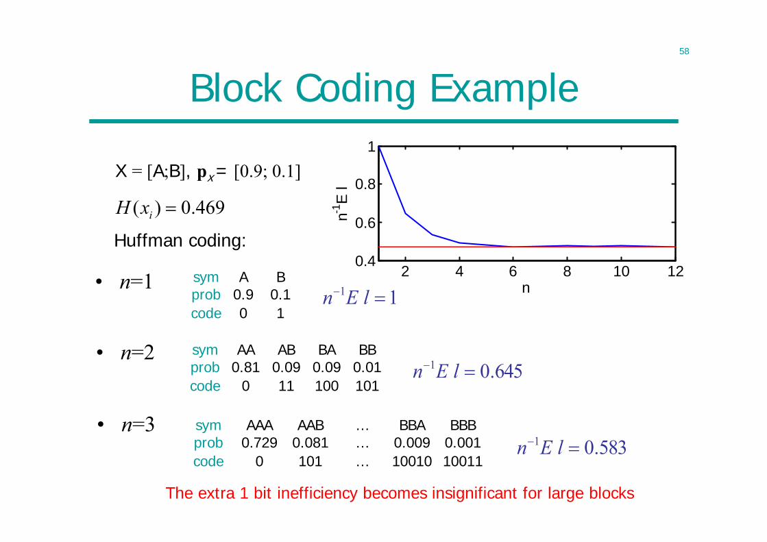
Block Coding Example
• n=1 sym A Bprob 0.9 0.1code 0 1
11 lEn
• n=2 sym AA AB BA BBprob 0.81 0.09 0.09 0.01code 0 11 100 101
645.01 lEn
• n=3 sym AAA AAB … BBA BBBprob 0.729 0.081 … 0.009 0.001code 0 101 … 10010 10011
583.01 lEn
2 4 6 8 10 120.4
0.6
0.8
1
n-1E
l
n
469.0)( ixH
X = [A;B], px = [0.9; 0.1]
Huffman coding:
The extra 1 bit inefficiency becomes insignificant for large blocks
59
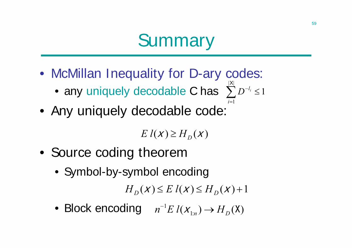
• McMillan Inequality for D-ary codes:• any uniquely decodable C has
• Any uniquely decodable code:
• Source coding theorem• Symbol-by-symbol encoding
• Block encoding
Summary
( ) ( )DE l Hx x
1||
1
X
i
liD
1)()()( xxx DD HlEH1
1:( ) ( )n Dn E l H x X
60
Lecture 5
• Source Coding Algorithms• Huffman Coding• Lempel-Ziv Coding
61
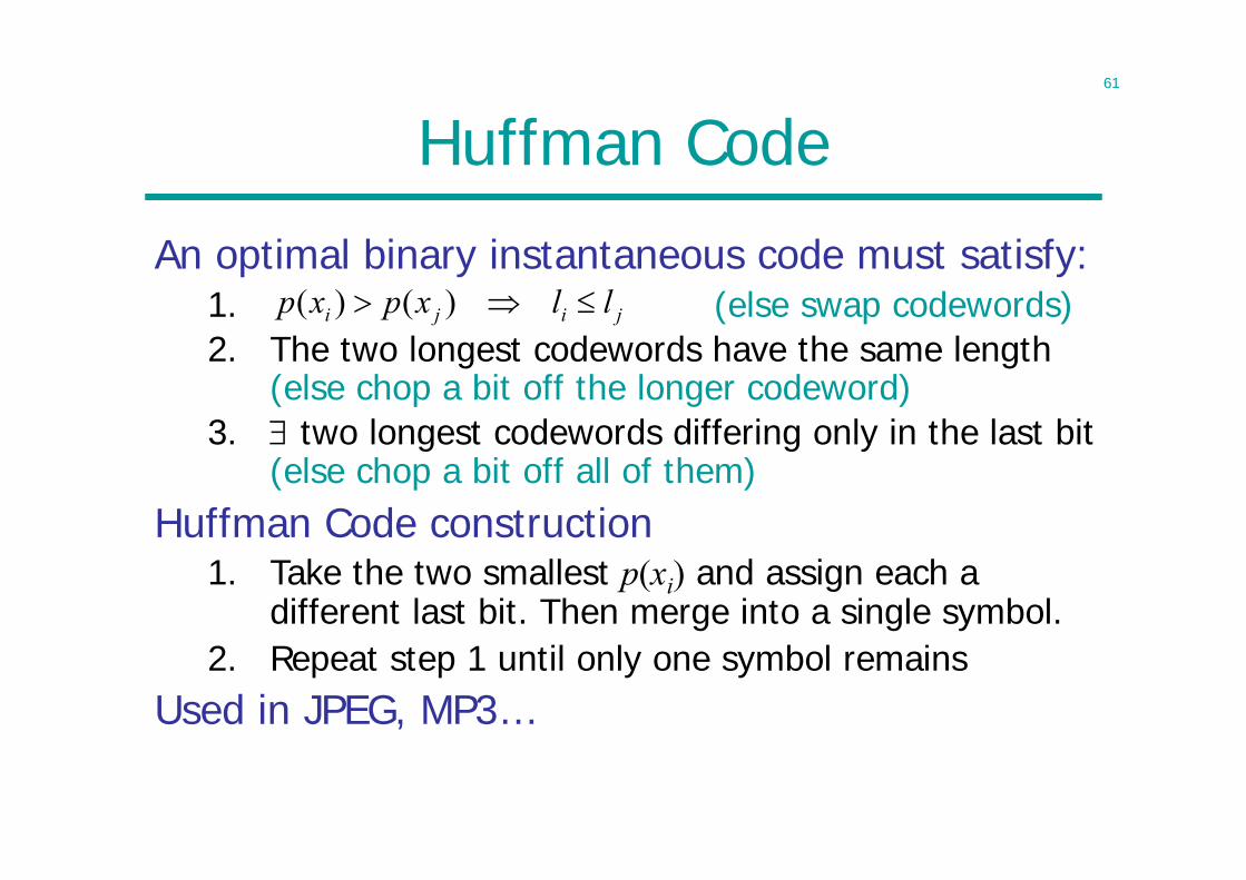
Huffman Code
An optimal binary instantaneous code must satisfy:1. (else swap codewords)jiji llxpxp )()(2. The two longest codewords have the same length
(else chop a bit off the longer codeword)3. two longest codewords differing only in the last bit
(else chop a bit off all of them)Huffman Code construction
1. Take the two smallest p(xi) and assign each a different last bit. Then merge into a single symbol.
2. Repeat step 1 until only one symbol remainsUsed in JPEG, MP3…
62
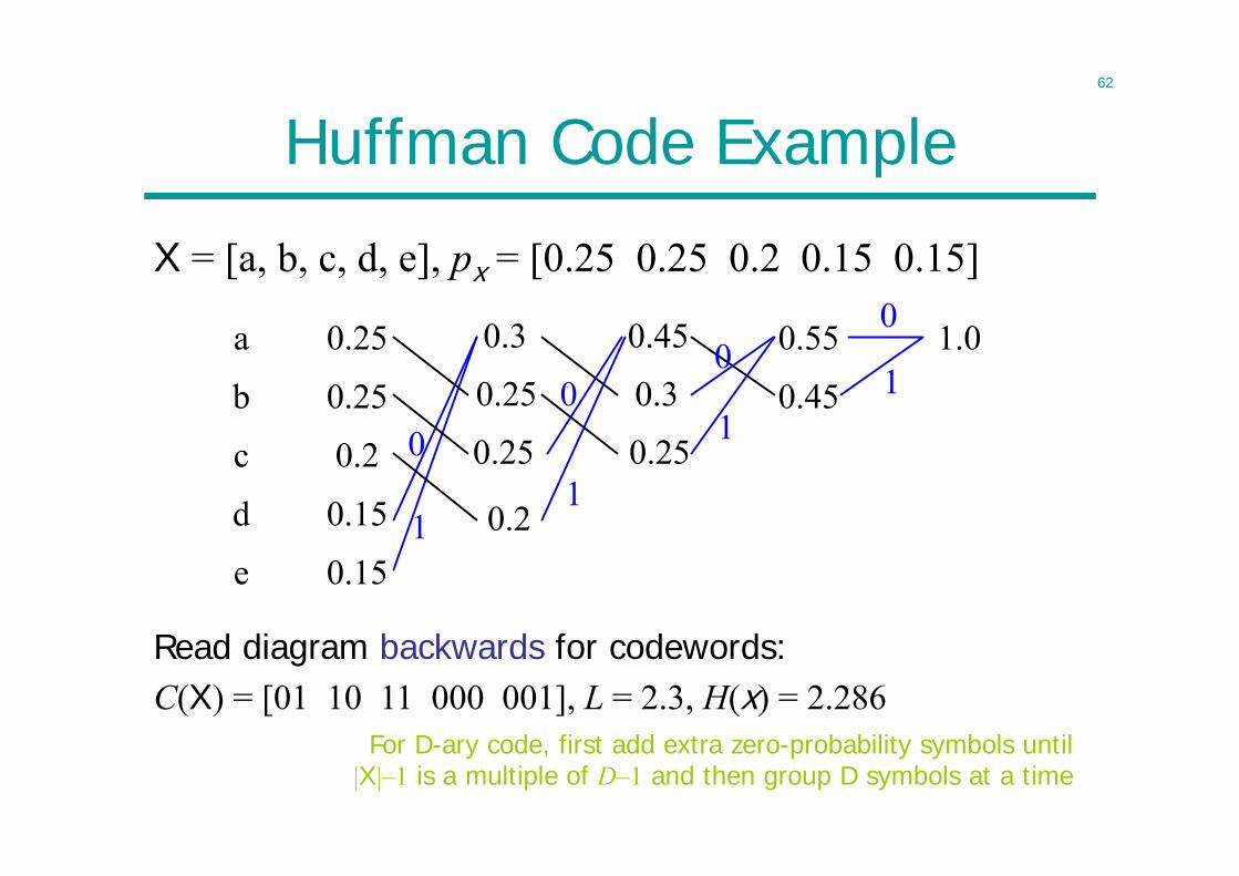
Huffman Code Example
X = [a, b, c, d, e], px = [0.25 0.25 0.2 0.15 0.15]
Read diagram backwards for codewords:C(X) = [01 10 11 000 001], L = 2.3, H(x) = 2.286
For D-ary code, first add extra zero-probability symbols until |X|–1 is a multiple of D–1 and then group D symbols at a time
63
Huffman Code is Optimal Instantaneous Code
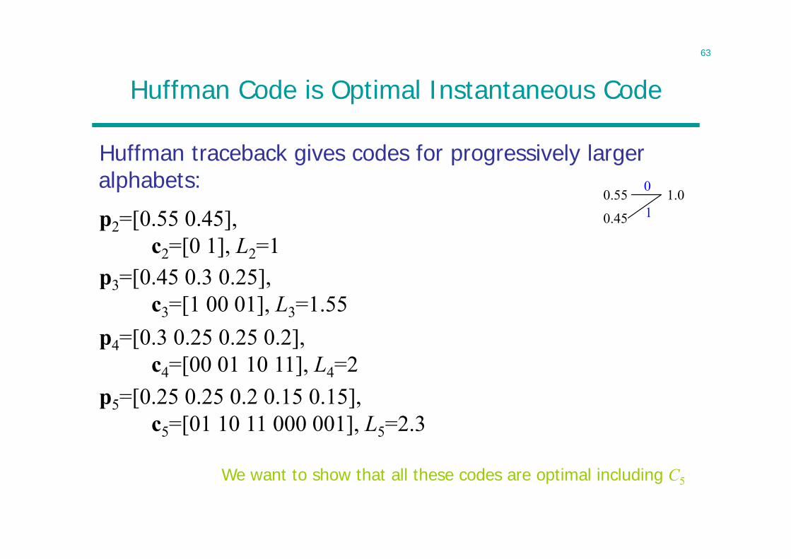
p2=[0.55 0.45],c2=[0 1], L2=1
0.25
0.25
0.2
0.15
0.15
0.25
0.25
0.2
0.3
0.25
0.45
0.3
0.55
0.45
1.0a
b
c
d
e
0
1
00 0
11
1
Huffman traceback gives codes for progressively larger alphabets:
We want to show that all these codes are optimal including C5
p3=[0.45 0.3 0.25],c3=[1 00 01], L3=1.55
p4=[0.3 0.25 0.25 0.2],c4=[00 01 10 11], L4=2
p5=[0.25 0.25 0.2 0.15 0.15],c5=[01 10 11 000 001], L5=2.3
64
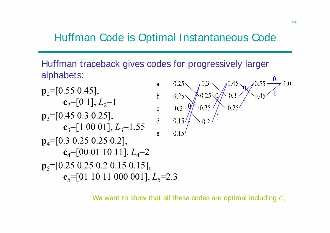
Huffman traceback gives codes for progressively larger alphabets:
Huffman Code is Optimal Instantaneous Code
p2=[0.55 0.45],c2=[0 1], L2=1
We want to show that all these codes are optimal including C5
p3=[0.45 0.3 0.25],c3=[1 00 01], L3=1.55
p4=[0.3 0.25 0.25 0.2],c4=[00 01 10 11], L4=2
p5=[0.25 0.25 0.2 0.15 0.15],c5=[01 10 11 000 001], L5=2.3
65
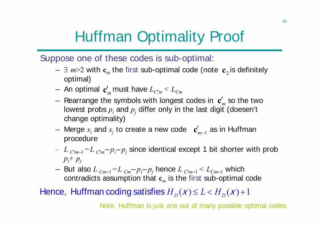
Suppose one of these codes is sub-optimal:– m>2 with cm the first sub-optimal code (note is definitely
optimal)
Huffman Optimality Proof
Note: Huffman is just one out of many possible optimal codes
2c
mcmc
1mc
– An optimal must have LC'm < LCm
– Rearrange the symbols with longest codes in so the two lowest probs pi and pj differ only in the last digit (doesen’t change optimality)
– Merge xi and xj to create a new code as in Huffman procedure
– L C'm–1 =L C'm– pi– pj since identical except 1 bit shorter with prob pi+ pj
– But also L Cm–1 =L Cm– pi– pj hence L C'm–1 < LCm–1 which contradicts assumption that cm is the first sub-optimal code
( ) ( ) 1D DH L H x xHence, Huffman coding satisfies
66
Shannon-Fano Code
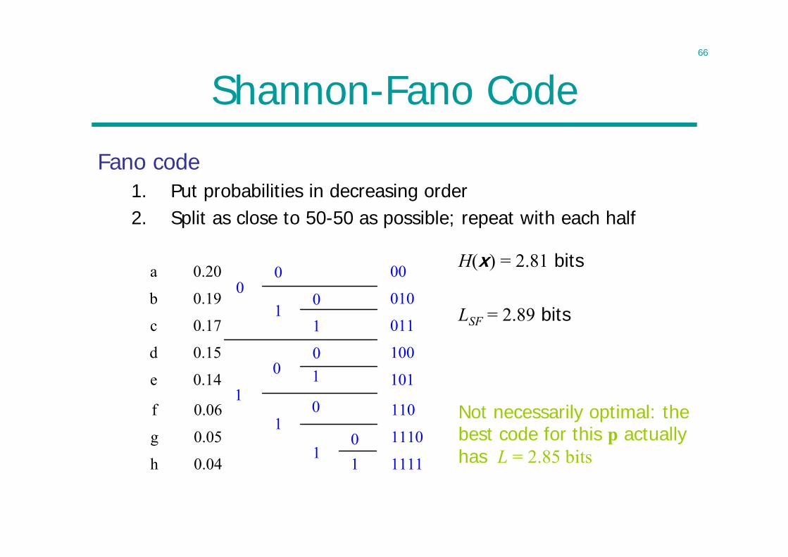
Fano code1. Put probabilities in decreasing order2. Split as close to 50-50 as possible; repeat with each half
0.20
0.19
0.17
0.15
0.14
a
b
c
d
e
0
10.06
0.05
0.04
f
g
h
0
10
1
0
1
01
0
101
00
010
011
100
101
110
1110
1111
H(x) = 2.81 bits
LSF = 2.89 bits
Not necessarily optimal: the best code for this p actually has L = 2.85 bits
67
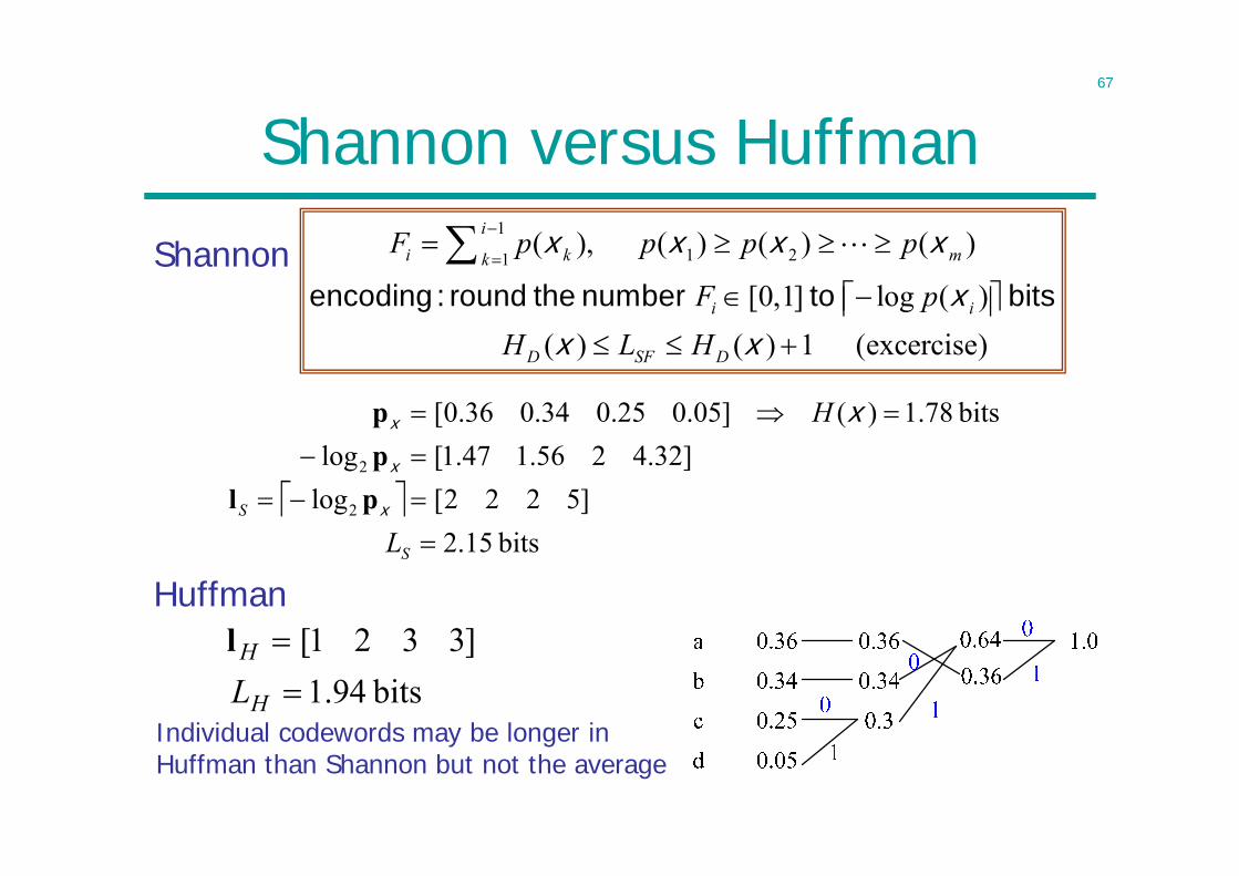
Shannon versus Huffman
Shannon
bits 15.2
]5222[log]32.4256.147.1[log
bits 78.1)(]05.025.034.036.0[
2
2
S
S
L
H
x
x
x x
plpp
Huffman
bits 94.1]3321[
H
H
Ll
Individual codewords may be longer in Huffman than Shannon but not the average
11 21
( ), ( ) ( ) ( )
[0,1] log ( )( ) ( ) 1 (excercise)
ii k mk
i i
D SF D
F p p p p
F pH L H
x x x x
xx x
encoding : round the number to bits
68
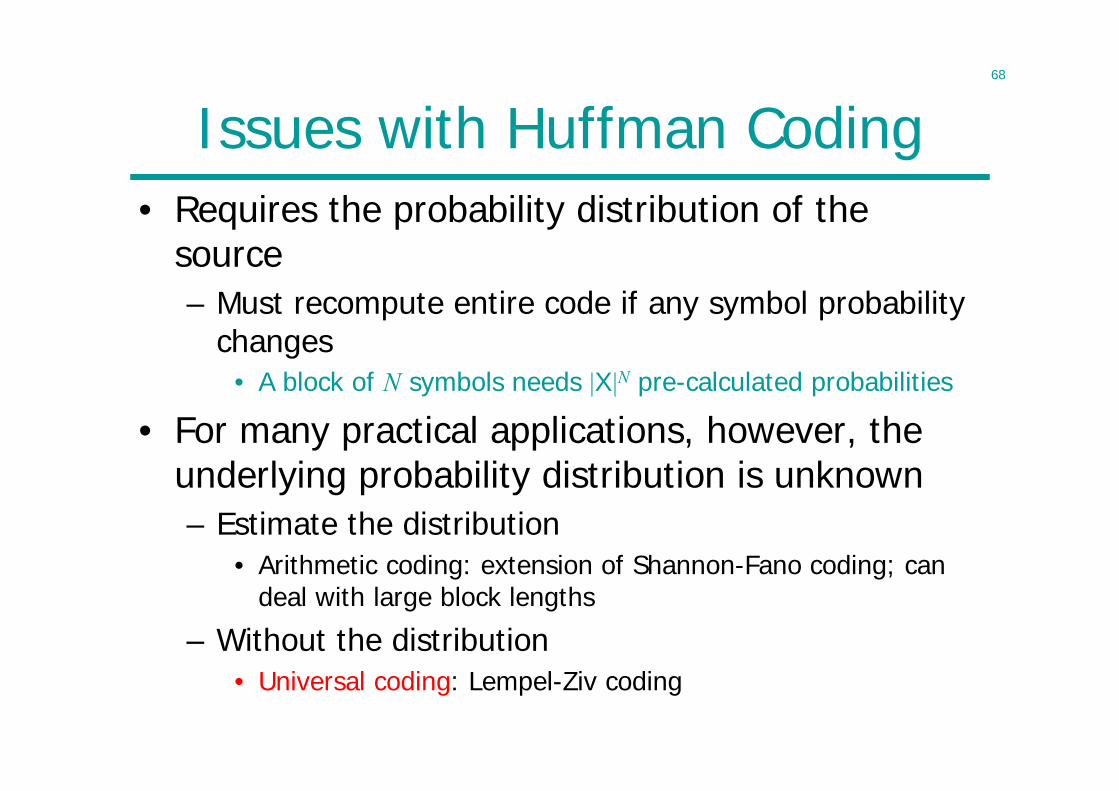
Issues with Huffman Coding• Requires the probability distribution of the
source– Must recompute entire code if any symbol probability
changes• A block of N symbols needs |X|N pre-calculated probabilities
• For many practical applications, however, the underlying probability distribution is unknown– Estimate the distribution
• Arithmetic coding: extension of Shannon-Fano coding; can deal with large block lengths
– Without the distribution• Universal coding: Lempel-Ziv coding
69
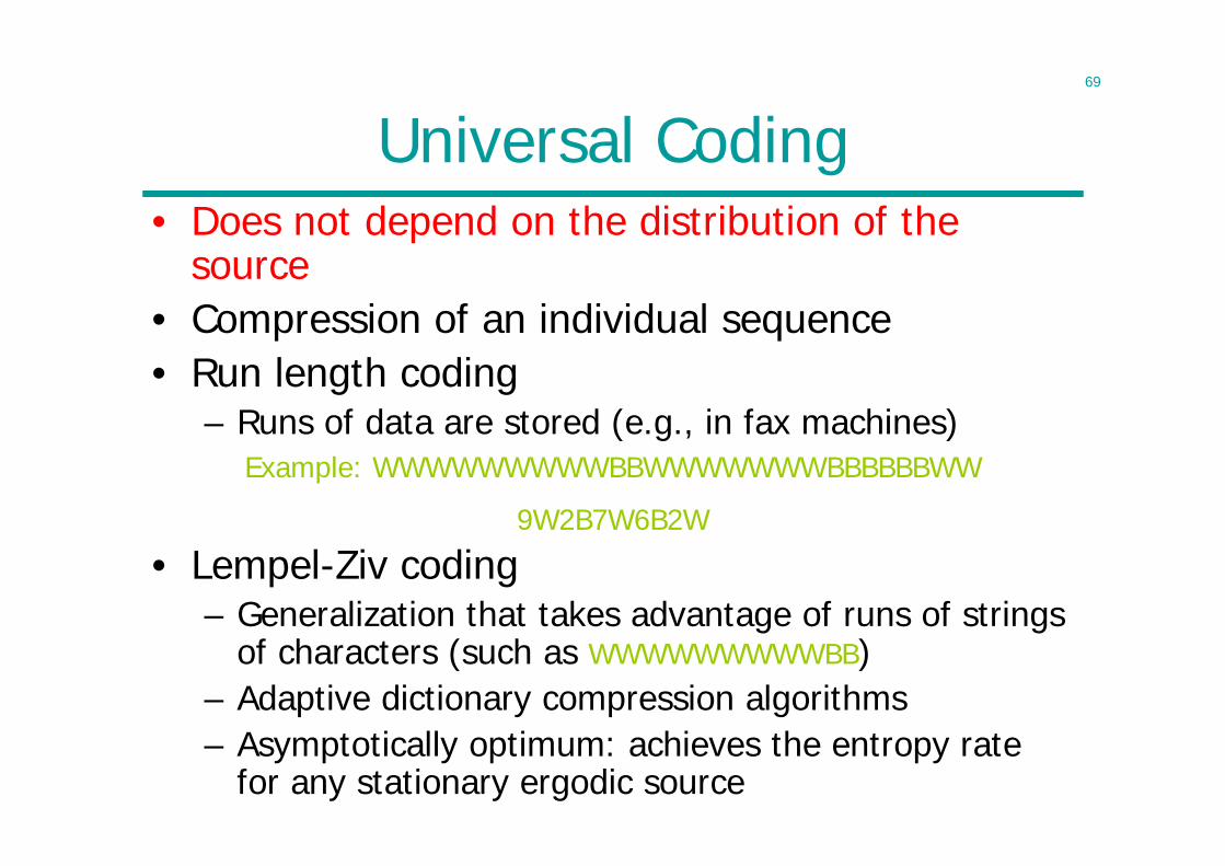
• Does not depend on the distribution of the source
• Compression of an individual sequence• Run length coding
– Runs of data are stored (e.g., in fax machines)
• Lempel-Ziv coding– Generalization that takes advantage of runs of strings
of characters (such as WWWWWWWWWBB)– Adaptive dictionary compression algorithms– Asymptotically optimum: achieves the entropy rate
for any stationary ergodic source
Universal Coding
Example: WWWWWWWWWBBWWWWWWWBBBBBBWW
9W2B7W6B2W
70
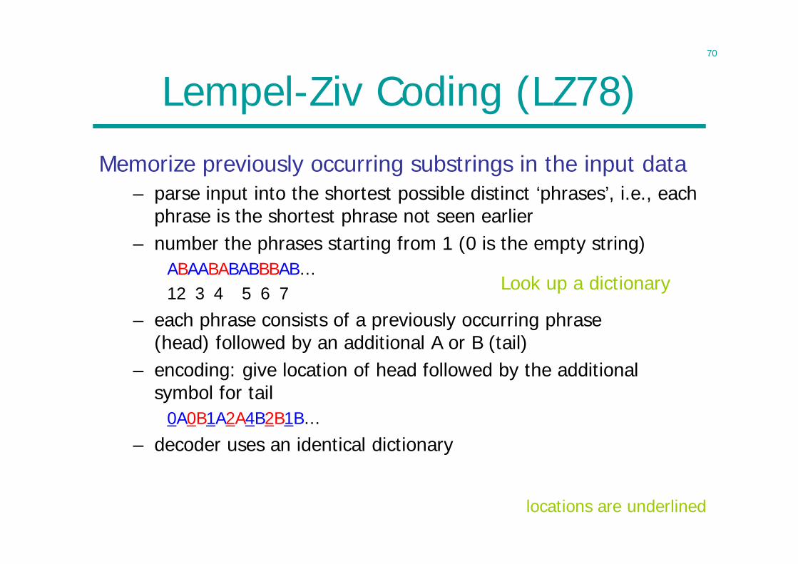
Lempel-Ziv Coding (LZ78)
Memorize previously occurring substrings in the input data– parse input into the shortest possible distinct ‘phrases’, i.e., each
phrase is the shortest phrase not seen earlier– number the phrases starting from 1 (0 is the empty string)
ABAABABABBBAB…12_3_4__5_6_7
– each phrase consists of a previously occurring phrase(head) followed by an additional A or B (tail)
– encoding: give location of head followed by the additional symbol for tail
0A0B1A2A4B2B1B…
– decoder uses an identical dictionary
locations are underlined
Look up a dictionary
71
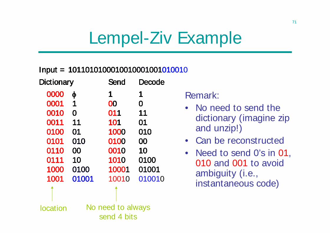
Input = 1011010100010010001001010010Dictionary Send Decode
0000 1 10001 1 00 00010 0 011 110011 11 101 010100 01 1000 0100101 010 0100 000110 00 0010 100111 10 1010 01001000 0100 10001 010011001 01001
Input = 1011010100010010001001010010Dictionary Send Decode
00 1 101 1 00 010 0
Input = 1011010100010010001001010010Dictionary Send Decode
00 1 101 1 00 010 0 011 11
Input = 1011010100010010001001010010Dictionary Send Decode
00 1 101 1 00 010 0 011 1111 11
Input = 1011010100010010001001010010Dictionary Send Decode
00 1 101 1 00 010 0 011 1111 11 101 01
Lempel-Ziv Example
Input = 1011010100010010001001010010Dictionary Send Decode
1 1
Input = 1011010100010010001001010010Dictionary Send Decode
0 1 11 1 00 0
Input = 1011010100010010001001010010Dictionary Send Decode
000 1 1001 1 00 0010 0 011 11011 11 101 01100 01
Input = 1011010100010010001001010010Dictionary Send Decode
000 1 1001 1 00 0010 0 011 11011 11 101 01100 01
Input = 1011010100010010001001010010Dictionary Send Decode
000 1 1001 1 00 0010 0 011 11011 11 101 01100 01 1000 010
Input = 1011010100010010001001010010Dictionary Send Decode
000 1 1001 1 00 0010 0 011 11011 11 101 01100 01 1000 010101 010
Input = 1011010100010010001001010010Dictionary Send Decode
000 1 1001 1 00 0010 0 011 11011 11 101 01100 01 1000 010101 010 0100 00
Input = 1011010100010010001001010010Dictionary Send Decode
000 1 1001 1 00 0010 0 011 11011 11 101 01100 01 1000 010101 010 0100 00110 00
Input = 1011010100010010001001010010Dictionary Send Decode
000 1 1001 1 00 0010 0 011 11011 11 101 01100 01 1000 010101 010 0100 00110 00 0010 10
Input = 1011010100010010001001010010Dictionary Send Decode
000 1 1001 1 00 0010 0 011 11011 11 101 01100 01 1000 010101 010 0100 00110 00 0010 10111 10
Input = 1011010100010010001001010010Dictionary Send Decode
000 1 1001 1 00 0010 0 011 11011 11 101 01100 01 1000 010101 010 0100 00110 00 0010 10111 10
Input = 1011010100010010001001010010Dictionary Send Decode
000 1 1001 1 00 0010 0 011 11011 11 101 01100 01 1000 010101 010 0100 00110 00 0010 10111 10
Input = 1011010100010010001001010010Dictionary Send Decode
000 1 1001 1 00 0010 0 011 11011 11 101 01100 01 1000 010101 010 0100 00110 00 0010 10111 10 1010 0100
Input = 1011010100010010001001010010Dictionary Send Decode
0000 1 10001 1 00 00010 0 011 110011 11 101 010100 01 1000 0100101 010 0100 000110 00 0010 100111 10 1010 01001000 0100
Input = 1011010100010010001001010010Dictionary Send Decode
0000 1 10001 1 00 00010 0 011 110011 11 101 010100 01 1000 0100101 010 0100 000110 00 0010 100111 10 1010 01001000 0100
Input = 1011010100010010001001010010Dictionary Send Decode
0000 1 10001 1 00 00010 0 011 110011 11 101 010100 01 1000 0100101 010 0100 000110 00 0010 100111 10 1010 01001000 0100
Input = 1011010100010010001001010010Dictionary Send Decode
0000 1 10001 1 00 00010 0 011 110011 11 101 010100 01 1000 0100101 010 0100 000110 00 0010 100111 10 1010 01001000 0100
Input = 1011010100010010001001010010Dictionary Send Decode
0000 1 10001 1 00 00010 0 011 110011 11 101 010100 01 1000 0100101 010 0100 000110 00 0010 100111 10 1010 01001000 0100 10001 01001
Input = 1011010100010010001001010010Dictionary Send Decode
0000 1 10001 1 00 00010 0 011 110011 11 101 010100 01 1000 0100101 010 0100 000110 00 0010 100111 10 1010 01001000 0100 10001 010011001 01001
Input = 1011010100010010001001010010Dictionary Send Decode
0000 1 10001 1 00 00010 0 011 110011 11 101 010100 01 1000 0100101 010 0100 000110 00 0010 100111 10 1010 01001000 0100 10001 010011001 01001
Input = 1011010100010010001001010010Dictionary Send Decode
0000 1 10001 1 00 00010 0 011 110011 11 101 010100 01 1000 0100101 010 0100 000110 00 0010 100111 10 1010 01001000 0100 10001 010011001 01001
Input = 1011010100010010001001010010Dictionary Send Decode
0000 1 10001 1 00 00010 0 011 110011 11 101 010100 01 1000 0100101 010 0100 000110 00 0010 100111 10 1010 01001000 0100 10001 010011001 01001
Input = 1011010100010010001001010010Dictionary Send Decode
0000 1 10001 1 00 00010 0 011 110011 11 101 010100 01 1000 0100101 010 0100 000110 00 0010 100111 10 1010 01001000 0100 10001 010011001 01001 10010 010010
Remark:• No need to send the
dictionary (imagine zip and unzip!)
• Can be reconstructed• Need to send 0’s in 01,
010 and 001 to avoid ambiguity (i.e., instantaneous code)
location No need to always send 4 bits
72
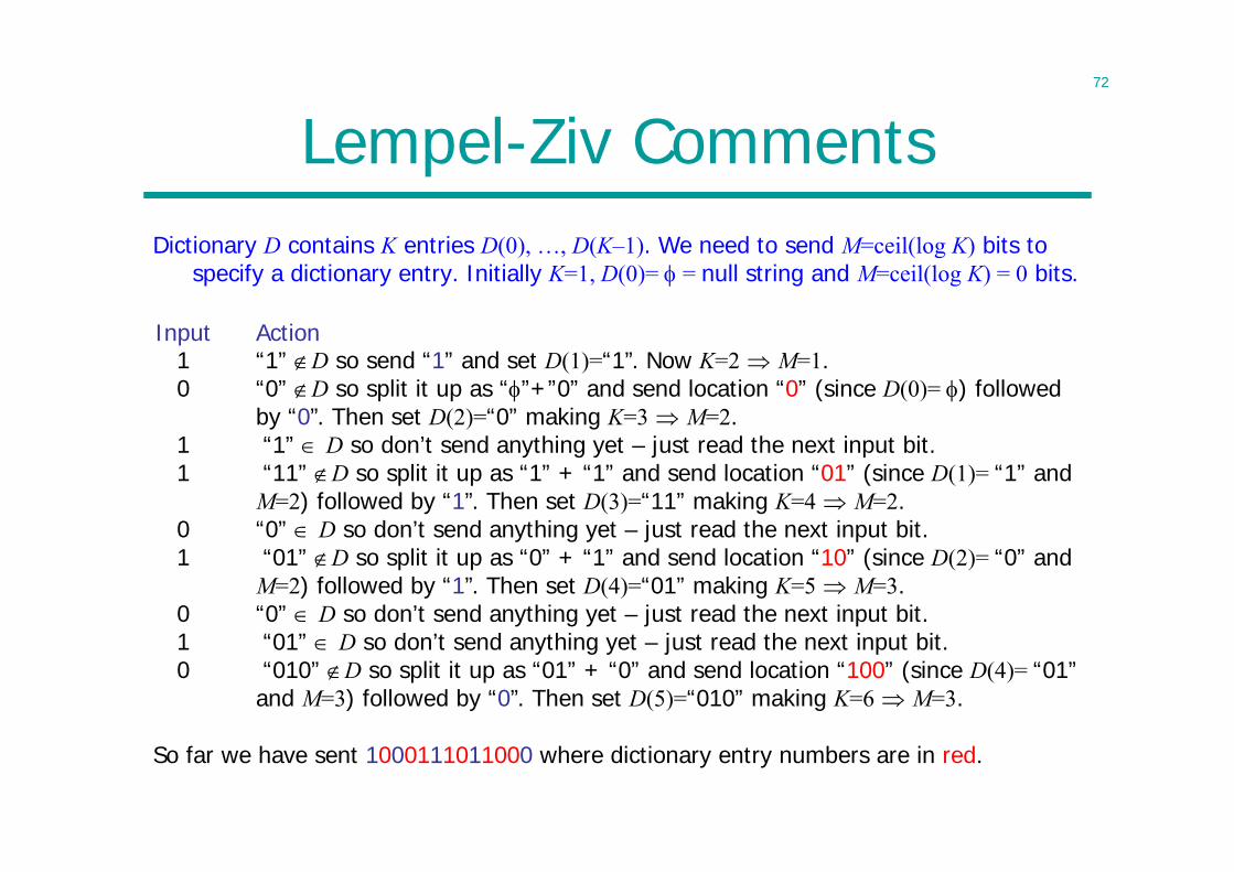
Lempel-Ziv CommentsDictionary D contains K entries D(0), …, D(K–1). We need to send M=ceil(log K) bits to
specify a dictionary entry. Initially K=1, D(0)= = null string and M=ceil(log K) = 0 bits.
Input Action1 “1” D so send “1” and set D(1)=“1”. Now K=2 M=1.0 “0” D so split it up as “”+”0” and send location “0” (since D(0)= ) followed
by “0”. Then set D(2)=“0” making K=3 M=2.1 “1” D so don’t send anything yet – just read the next input bit.1 “11” D so split it up as “1” + “1” and send location “01” (since D(1)= “1” and
M=2) followed by “1”. Then set D(3)=“11” making K=4 M=2.0 “0” D so don’t send anything yet – just read the next input bit.1 “01” D so split it up as “0” + “1” and send location “10” (since D(2)= “0” and
M=2) followed by “1”. Then set D(4)=“01” making K=5 M=3.0 “0” D so don’t send anything yet – just read the next input bit.1 “01” D so don’t send anything yet – just read the next input bit.0 “010” D so split it up as “01” + “0” and send location “100” (since D(4)= “01”
and M=3) followed by “0”. Then set D(5)=“010” making K=6 M=3.
So far we have sent 1000111011000 where dictionary entry numbers are in red.
73
Lempel-Ziv Properties• Simple to implement• Widely used because of its speed and efficiency
– applications: compress, gzip, GIF, TIFF, modem …– variations: LZW (considering last character of the
current phrase as part of the next phrase, used in Adobe Acrobat), LZ77 (sliding window)
– different dictionary handling, etc• Excellent compression in practice
– many files contain repetitive sequences– worse than arithmetic coding for text files
74
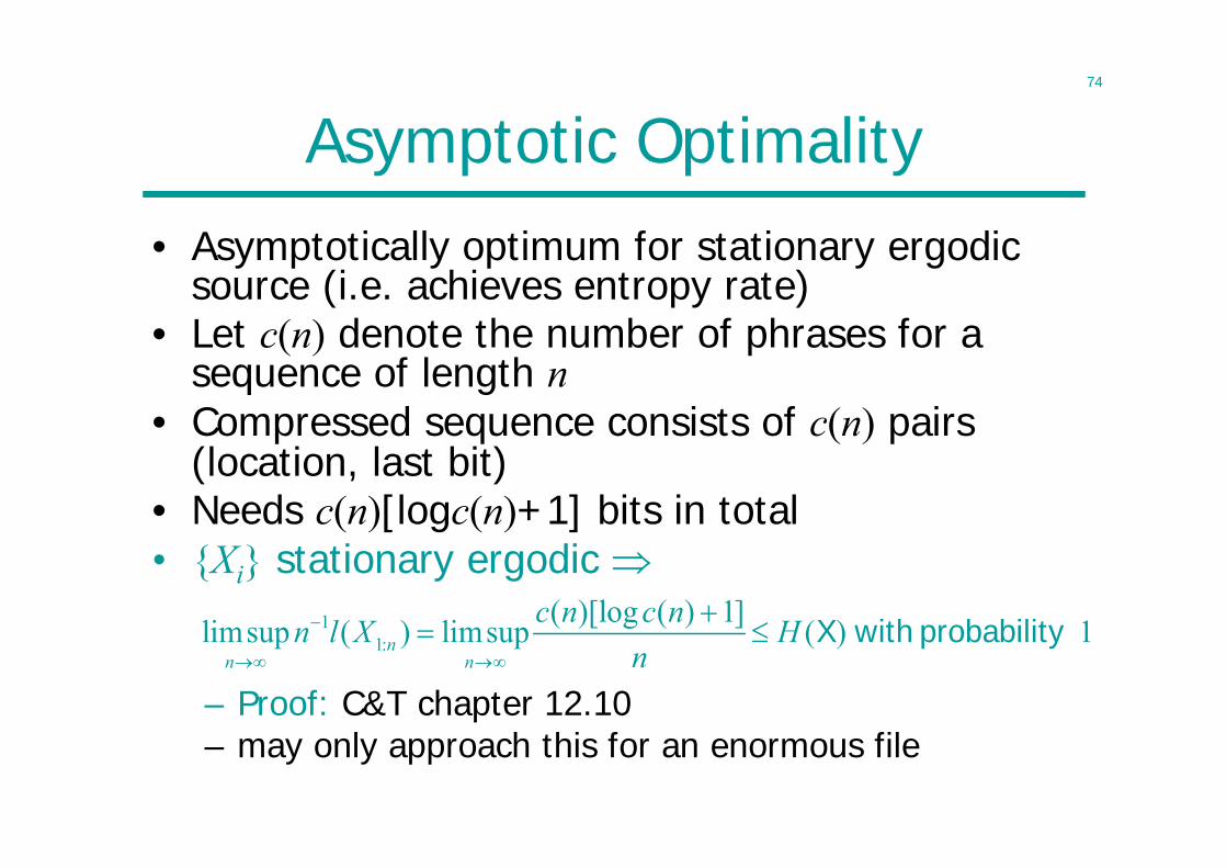
Asymptotic Optimality• Asymptotically optimum for stationary ergodic
source (i.e. achieves entropy rate)• Let c(n) denote the number of phrases for a
sequence of length n• Compressed sequence consists of c(n) pairs
(location, last bit)• Needs c(n)[logc(n)+1] bits in total• {Xi} stationary ergodic
– Proof: C&T chapter 12.10– may only approach this for an enormous file
11:
( )[log ( ) 1]limsup ( ) limsup ( ) 1nn n
c n c nn l X Hn
X with probability
75
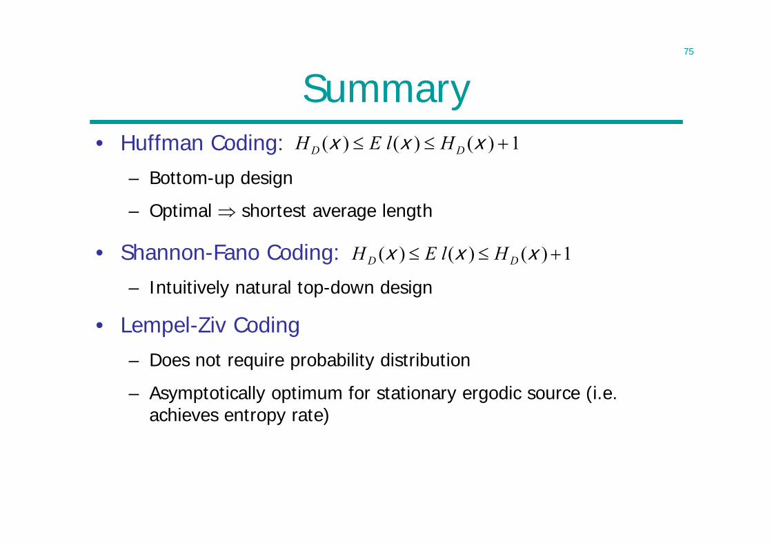
• Shannon-Fano Coding:– Intuitively natural top-down design
• Lempel-Ziv Coding– Does not require probability distribution
– Asymptotically optimum for stationary ergodic source (i.e. achieves entropy rate)
• Huffman Coding:– Bottom-up design
– Optimal shortest average length
Summary
1)()()( xxx DD HlEH
1)()()( xxx DD HlEH
76
Lecture 6
• Markov Chains– Have a special meaning– Not to be confused with the standard
definition of Markov chains (which are sequences of discrete random variables)
• Data Processing Theorem– You can’t create information from nothing
• Fano’s Inequality– Lower bound for error in estimating X from Y
77
Markov Chains
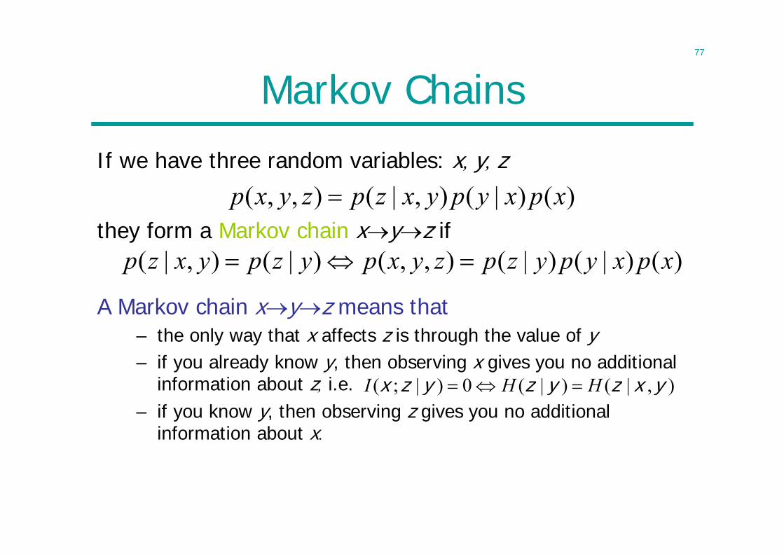
If we have three random variables: x, y, z)()|(),|(),,( xpxypyxzpzyxp
they form a Markov chain xyz if)()|()|(),,()|(),|( xpxypyzpzyxpyzpyxzp
A Markov chain xyz means that– the only way that x affects z is through the value of y
),|()|(0)|;( yxzyzyzx HHI – if you already know y, then observing x gives you no additional
information about z, i.e.– if you know y, then observing z gives you no additional
information about x.
78
Data Processing
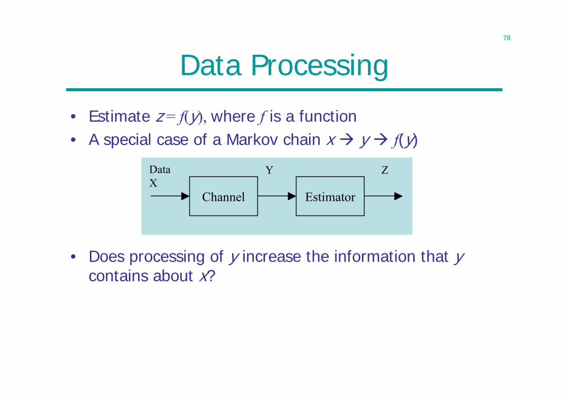
• Estimate z = f(y), where f is a function• A special case of a Markov chain x y f(y)
• Does processing of y increase the information that ycontains about x?
Channel Estimator
Data X
Y Z
79
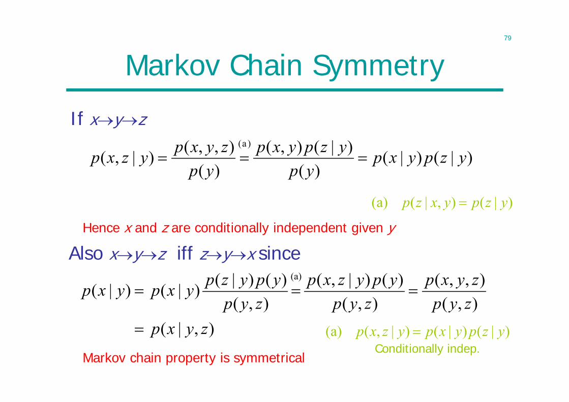
Markov Chain Symmetry
If xyz
)|()|()(
)|(),()(
),,()|,()a(
yzpyxpyp
yzpyxpyp
zyxpyzxp
)|(),|((a) yzpyxzp
Also xyz iff zyx since
),|(),(),,(
),()()|,(
),()()|()|()|(
(a)
zyxpzypzyxp
zypypyzxp
zypypyzpyxpyxp
Hence x and z are conditionally independent given y
Markov chain property is symmetrical
)|()|()|,((a) yzpyxpyzxp Conditionally indep.
80
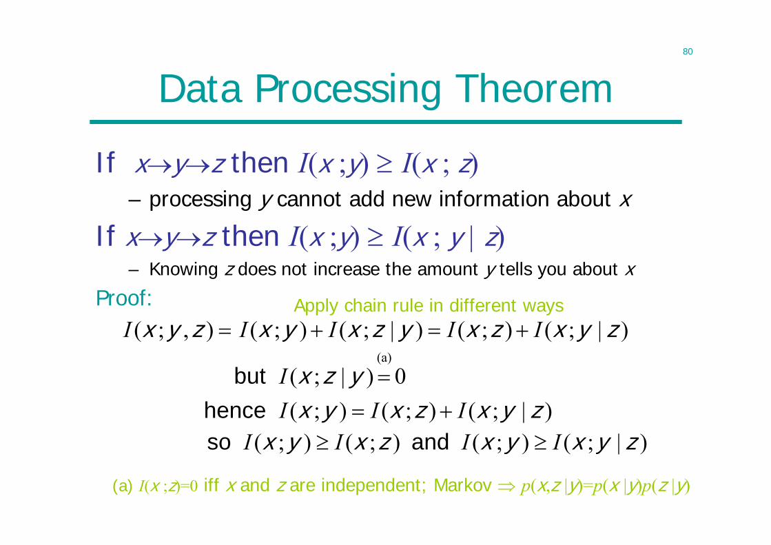
Data Processing Theorem
If xyz then I(x ;y) I(x ; z)– processing y cannot add new information about x
)|;();();(0)|;(
(a)
zyxzxyxyzx
IIII
hence but
(a) I(x ;z)=0 iff x and z are independent; Markov p(x,z |y)=p(x |y)p(z |y)
If xyz then I(x ;y) I(x ; y | z)– Knowing z does not increase the amount y tells you about x
Proof:)|;();()|;();(),;( zyxzxyzxyxzyx IIIII
)|;();();();( zyxyxzxyx IIII and so
Apply chain rule in different ways
81
So Why Processing?
• One can not create information by manipulating the data
• But no information is lost if equality holds• Sufficient statistic
– z contains all the information in y about x– Preserves mutual information I(x ;y) = I(x ; z)
• The estimator should be designed in a way such that it outputs sufficient statistics
• Can the estimation be arbitrarily accurate?
82
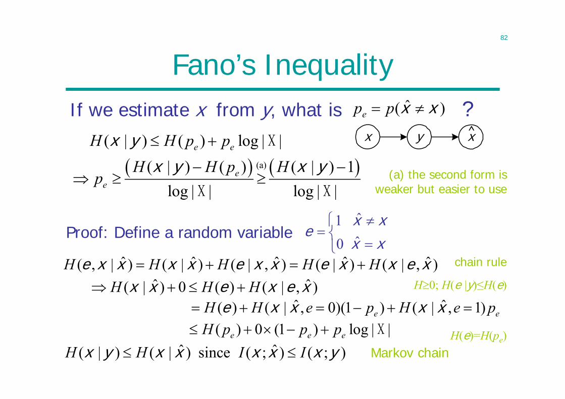
Fano’s InequalityIf we estimate x from y, what is ?
x xy ^
)ˆ( xx ppe
(a)
( | ) ( ) log | |( | ) ( ) ( | ) 1
log | | log | |
e e
ee
H H p pH H p H
p
X
X X
x yx y x y
Proof: Define a random variableˆ1ˆ0
x xe
x x
( ) 0 (1 ) log | |e e eH p p p X
(a) the second form is weaker but easier to use
chain rule
H0; H(e |y)≤H(e)
H(e)=H(pe)
ˆ ˆ ˆ ˆ ˆ( , | ) ( | ) ( | , ) ( | ) ( | , )H H H H H e x x x x e x x e x x e xˆ ˆ( | ) 0 ( ) ( | , )H H H x x e x e x
ˆ ˆ( ) ( | , 0)(1 ) ( | , 1)e eH H e p H e p e x x x x
ˆ ˆ( | ) ( | ) since ( ; ) ( ; )H H I I x y x x x x x y Markov chain
83
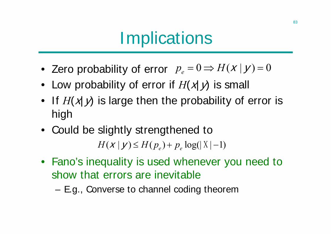
Implications
• Zero probability of error• Low probability of error if H(x|y) is small• If H(x|y) is large then the probability of error is
high• Could be slightly strengthened to
• Fano’s inequality is used whenever you need to show that errors are inevitable– E.g., Converse to channel coding theorem
0 ( | ) 0ep H x y
( | ) ( ) log(| | 1)e eH H p p Xx y
84
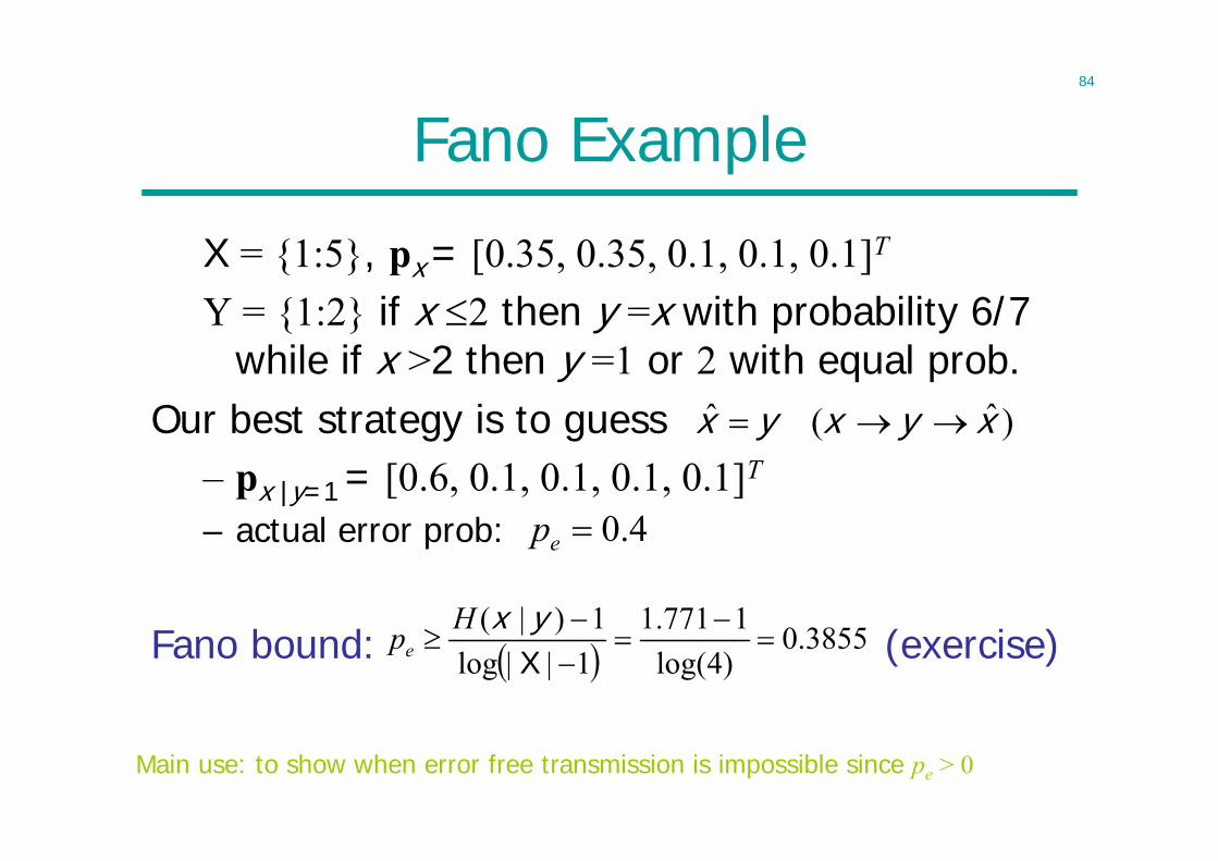
Fano Example
X = {1:5}, px = [0.35, 0.35, 0.1, 0.1, 0.1]T
Y = {1:2} if x 2 then y =x with probability 6/7 while if x >2 then y =1 or 2 with equal prob.
Our best strategy is to guess – px |y=1 = [0.6, 0.1, 0.1, 0.1, 0.1]T
– actual error prob:
Fano bound: (exercise) 3855.0)4log(1771.1
1||log1)|(
XyxHpe
Main use: to show when error free transmission is impossible since pe > 0
ˆ ˆ( ) x y x y x
4.0ep
85
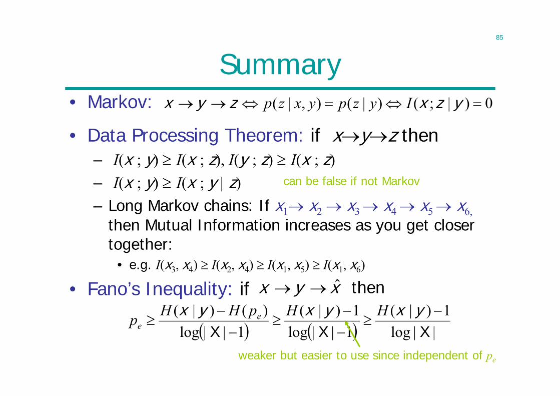
Summary• Markov:
• Data Processing Theorem: if xyz then– I(x ; y) I(x ; z), I(y ; z) I(x ; z)– I(x ; y) I(x ; y | z)– Long Markov chains: If x1 x2 x3 x4 x5 x6,
then Mutual Information increases as you get closer together:
• e.g. I(x3, x4) I(x2, x4) I(x1, x5) I(x1, x6)
• Fano’s Inequality: if
can be false if not Markov
then xyx ˆ
||log1)|(
1||log1)|(
1||log)()|(
XXX
yxyxyx HHpHHp ee
0)|;()|(),|( yzxzyx Iyzpyxzp
weaker but easier to use since independent of pe
86
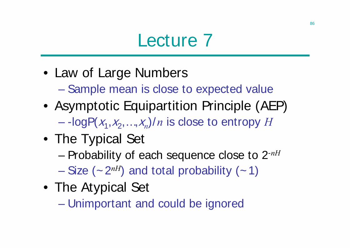
Lecture 7
• Law of Large Numbers– Sample mean is close to expected value
• Asymptotic Equipartition Principle (AEP)– -logP(x1,x2,…,xn)/n is close to entropy H
• The Typical Set– Probability of each sequence close to 2-nH
– Size (~2nH) and total probability (~1)• The Atypical Set
– Unimportant and could be ignored
87
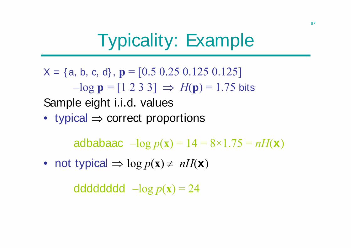
Typicality: Example
X = {a, b, c, d}, p = [0.5 0.25 0.125 0.125]–log p = [1 2 3 3] H(p) = 1.75 bits
Sample eight i.i.d. values• typical correct proportions
adbabaac –log p(x) = 14 = 8×1.75 = nH(x)
• not typical log p(x) nH(x)
dddddddd –log p(x) = 24
88
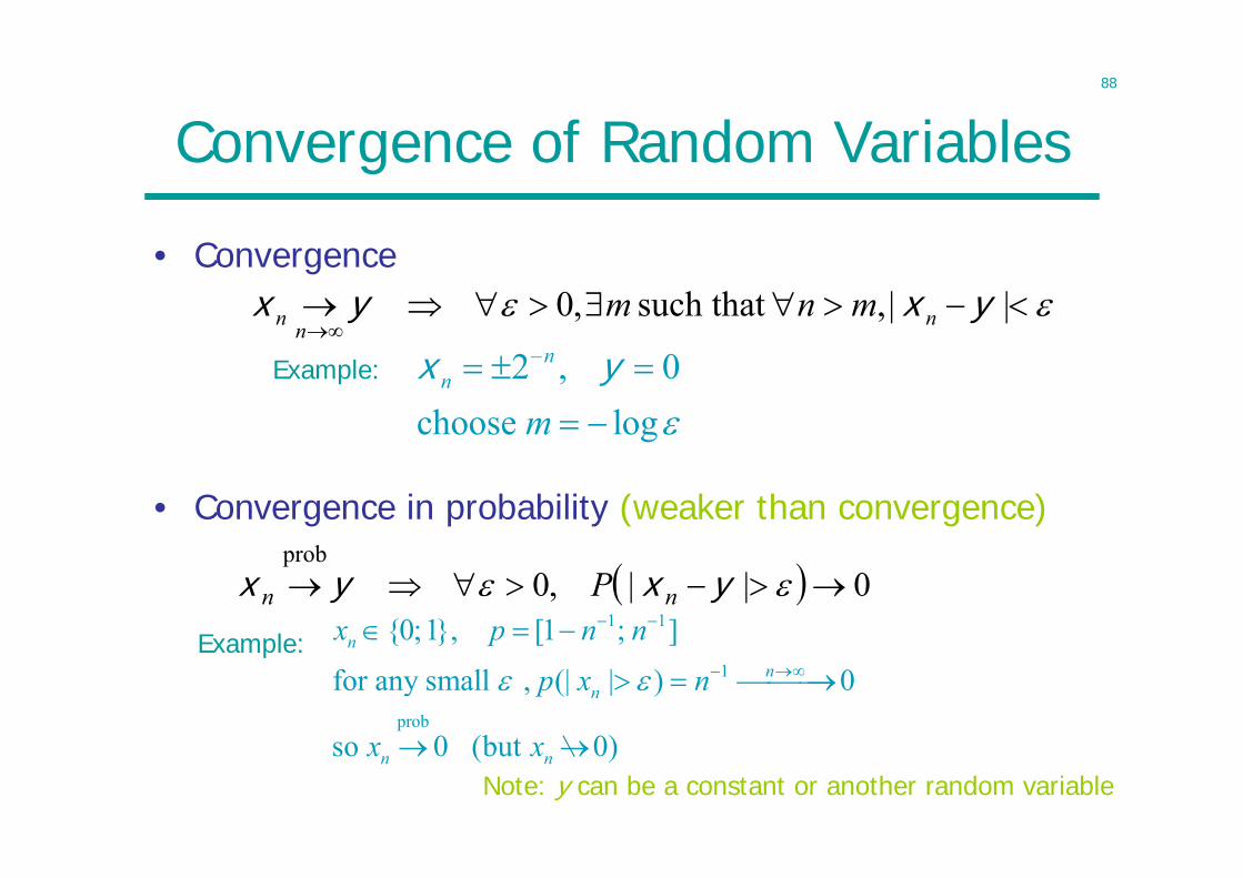
Convergence of Random Variables
• Convergence
||,such that ,0 yxyx nnn mnm
0||,0prob
yxyx nn P
Note: y can be a constant or another random variable
–2 , 0choose log
nn
m
x yExample:
1 1
1
prob
{0;1}, [1 ; ]
for any small , (| | ) 0
so 0 (but 0)
nn
n
n n
x p n n
p x n
x x
Example:
• Convergence in probability (weaker than convergence)
89
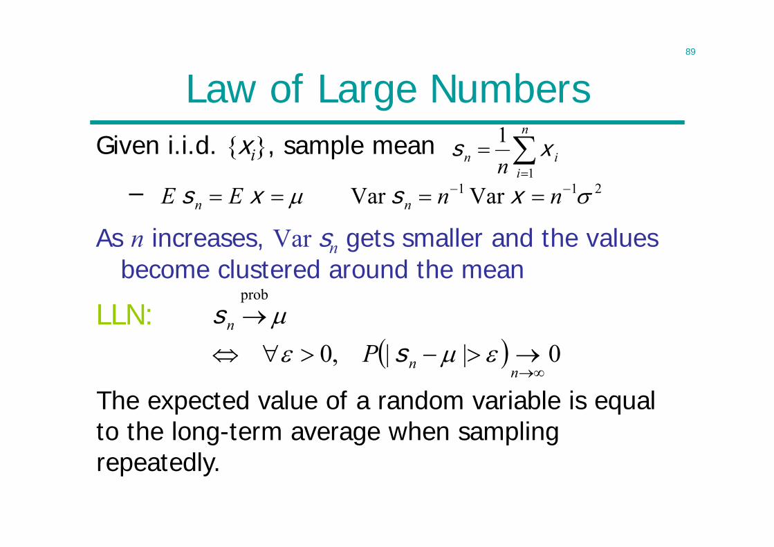
Law of Large NumbersGiven i.i.d. {xi}, sample mean
–
As n increases, Var sn gets smaller and the values become clustered around the mean
n
iin n 1
1 xs
211 VarVar nnEE nn xsxs
0||,0
prob
nn
n
P
ssLLN:
The expected value of a random variable is equal to the long-term average when sampling repeatedly.
90
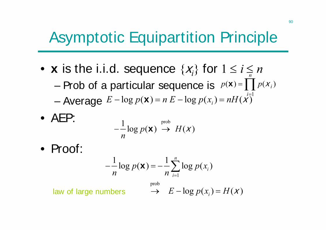
Asymptotic Equipartition Principle
• x is the i.i.d. sequence {xi} for 1 i n– Prob of a particular sequence is– Average
• AEP:
• Proof:
prob1 log ( ) ( )p Hn
xx
n
iipp
1
)()( xx
)()(log)(log xnHxpEnpE i x
1prob
1 1log ( ) log ( )
log ( ) ( )
n
ii
i
p p xn n
E p x H
x
x
law of large numbers
91
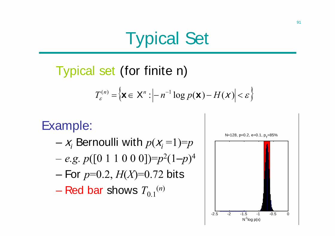
Typical Set
Typical set (for finite n)
Example:– xi Bernoulli with p(xi =1)=p– e.g. p([0 1 1 0 0 0])=p2(1–p)4
– For p=0.2, H(X)=0.72 bits– Red bar shows T0.1
(n)
)()(log: 1)( xHpnT nn xx X
-2.5 -2 -1.5 -1 -0.5 0N-1log p(x)
N=1, p=0.2, e=0.1, pT=0%
-2.5 -2 -1.5 -1 -0.5 0N-1log p(x)
N=2, p=0.2, e=0.1, pT=0%
-2.5 -2 -1.5 -1 -0.5 0N-1log p(x)
N=4, p=0.2, e=0.1, pT=41%
-2.5 -2 -1.5 -1 -0.5 0N-1log p(x)
N=8, p=0.2, e=0.1, pT=29%
-2.5 -2 -1.5 -1 -0.5 0N-1log p(x)
N=16, p=0.2, e=0.1, pT=45%
-2.5 -2 -1.5 -1 -0.5 0N-1log p(x)
N=32, p=0.2, e=0.1, pT=62%
-2.5 -2 -1.5 -1 -0.5 0N-1log p(x)
N=64, p=0.2, e=0.1, pT=72%
-2.5 -2 -1.5 -1 -0.5 0N-1log p(x)
N=128, p=0.2, e=0.1, pT=85%
92
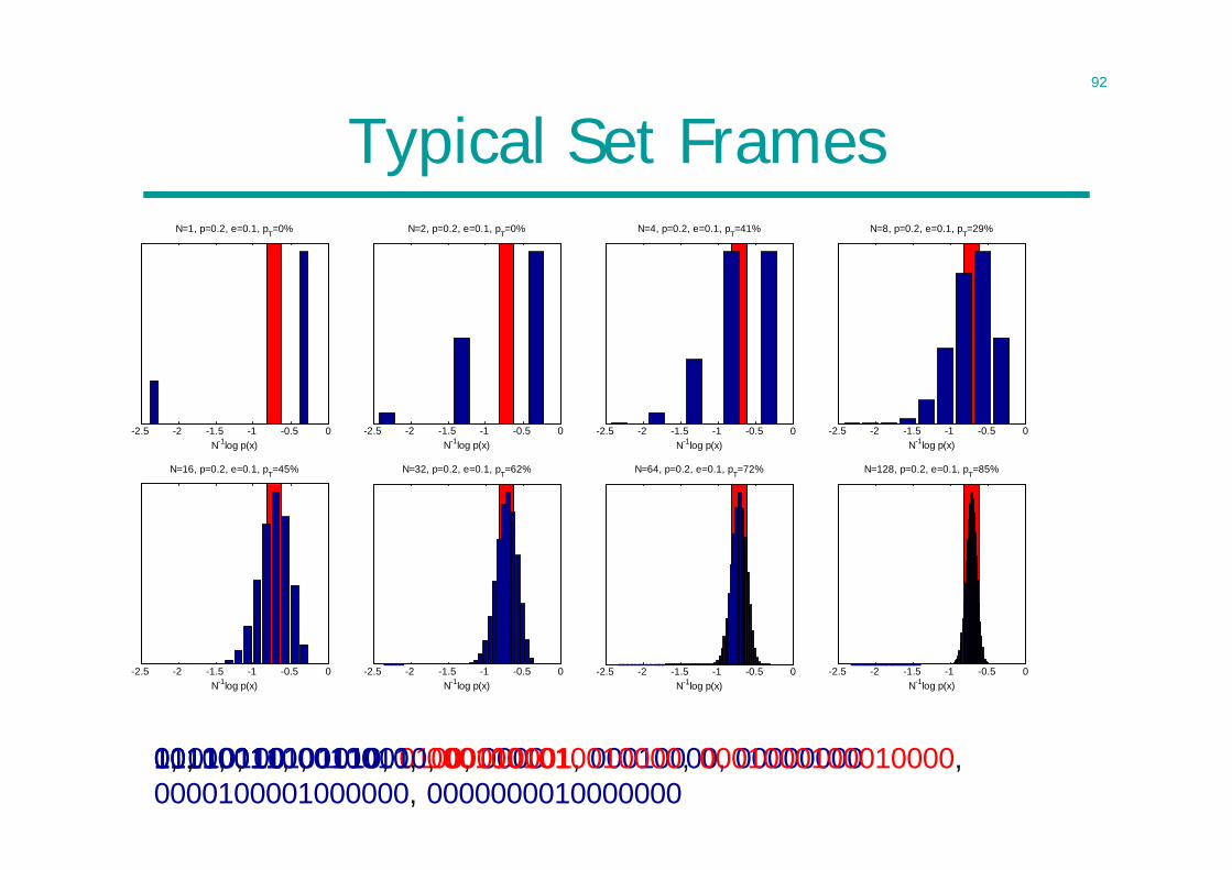
1111, 1101, 1010, 0100, 000000110011, 00110010, 00010001, 00010000, 000000000010001100010010, 0001001010010000, 0001000100010000, 0000100001000000, 00000000100000001, 011, 10, 00
Typical Set Frames
-2.5 -2 -1.5 -1 -0.5 0N-1log p(x)
N=1, p=0.2, e=0.1, pT=0%
-2.5 -2 -1.5 -1 -0.5 0N-1log p(x)
N=2, p=0.2, e=0.1, pT=0%
-2.5 -2 -1.5 -1 -0.5 0N-1log p(x)
N=4, p=0.2, e=0.1, pT=41%
-2.5 -2 -1.5 -1 -0.5 0N-1log p(x)
N=8, p=0.2, e=0.1, pT=29%
-2.5 -2 -1.5 -1 -0.5 0N-1log p(x)
N=16, p=0.2, e=0.1, pT=45%
-2.5 -2 -1.5 -1 -0.5 0N-1log p(x)
N=32, p=0.2, e=0.1, pT=62%
-2.5 -2 -1.5 -1 -0.5 0N-1log p(x)
N=64, p=0.2, e=0.1, pT=72%
-2.5 -2 -1.5 -1 -0.5 0N-1log p(x)
N=128, p=0.2, e=0.1, pT=85%
93
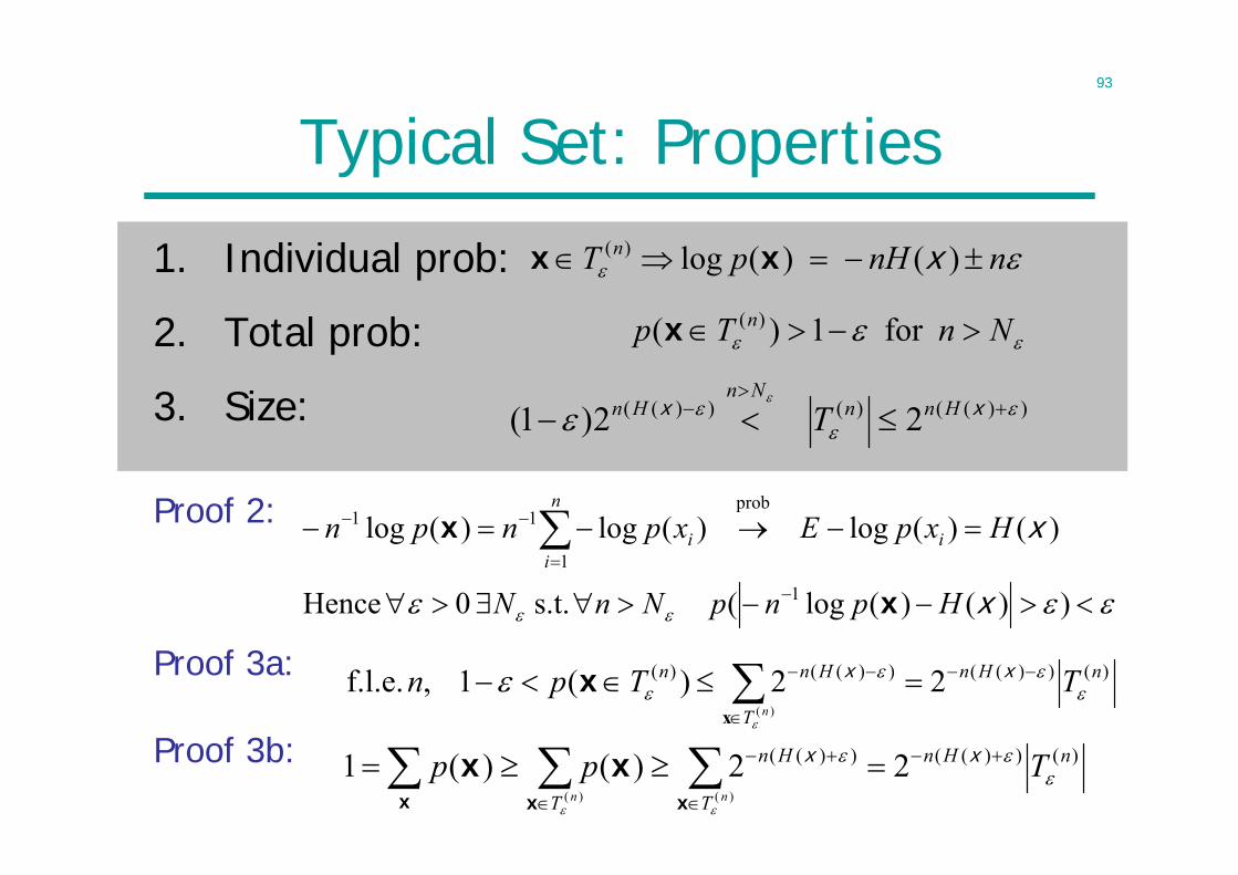
Typical Set: Properties
1. Individual prob:
2. Total prob:
3. Size:
nnHpT n )()(log)( xxx
NnTp n for 1)( )(x
))()(log( s.t. 0 Hence
)()(log)(log)(log
1
prob
1
11
x
x
HpnpNnN
HxpExpnpn i
n
ii
x
x
22)1( ))(()())((
xx HnnNn
Hn T
)())(())(( 22)()(1)()(
nHn
T
Hn
T
Tppnn
xx
xxx
xx
)())(())(()( 22)(1, f.l.e.)(
nHn
T
Hnn TTpnn
xx
x
x
Proof 2:
Proof 3a:
Proof 3b:
94
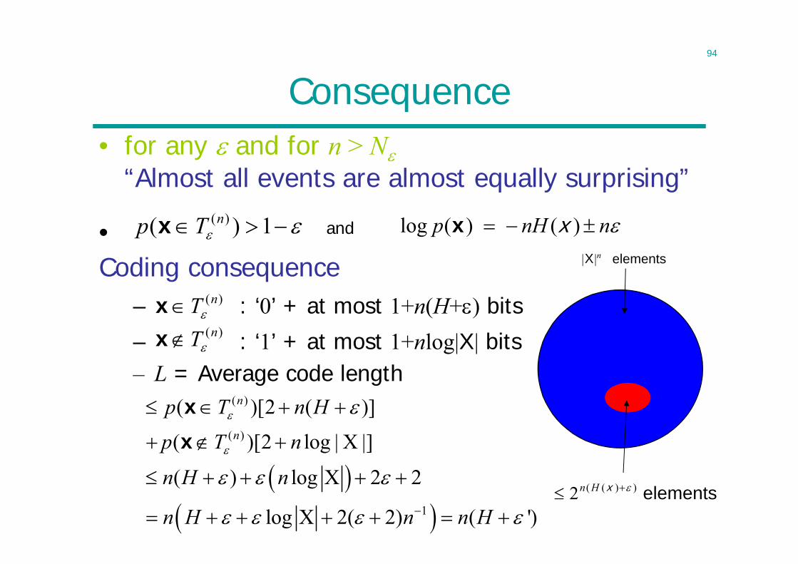
Consequence• for any and for n > N
“Almost all events are almost equally surprising”
• 1)( )(nTp x and
)(nTx)(nTx
( )
( )
1
( )[2 ( )]
( )[2 log | X |]
( ) log X 2 2
log X 2( 2) ( ')
n
n
p T n H
p T n
n H n
n H n n H
x
x
nnHp )()(log xx
Coding consequence– : ‘0’ + at most 1+n(H+) bits
– : ‘1’ + at most 1+nlog|X| bits– L = Average code length
elements ))((2 xHn
|X|n elements
95
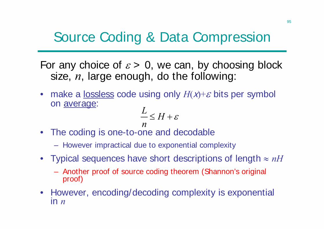
Source Coding & Data Compression
For any choice of > 0, we can, by choosing block size, n, large enough, do the following:
• make a lossless code using only H(x)+ bits per symbol on average:
• The coding is one-to-one and decodable– However impractical due to exponential complexity
• Typical sequences have short descriptions of length nH– Another proof of source coding theorem (Shannon’s original
proof)
• However, encoding/decoding complexity is exponential in n
L Hn
96
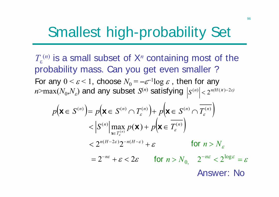
Smallest high-probability Set
T(n) is a small subset of Xn containing most of the
probability mass. Can you get even smaller ?
ε)n(HnS 2)()( 2 x
)()()()()( nnnnn TSpTSpSp xxx
Answer: No log
,0 22 nNnfor
Nn for
For any 0 < < 1, choose N0 = ––1log , then for any n>max(N0,N) and any subset S(n) satisfying
)()( )(max)(
n
T
n TppSn
xxx
)()2( 22 HnHn
22 n
97
Summary
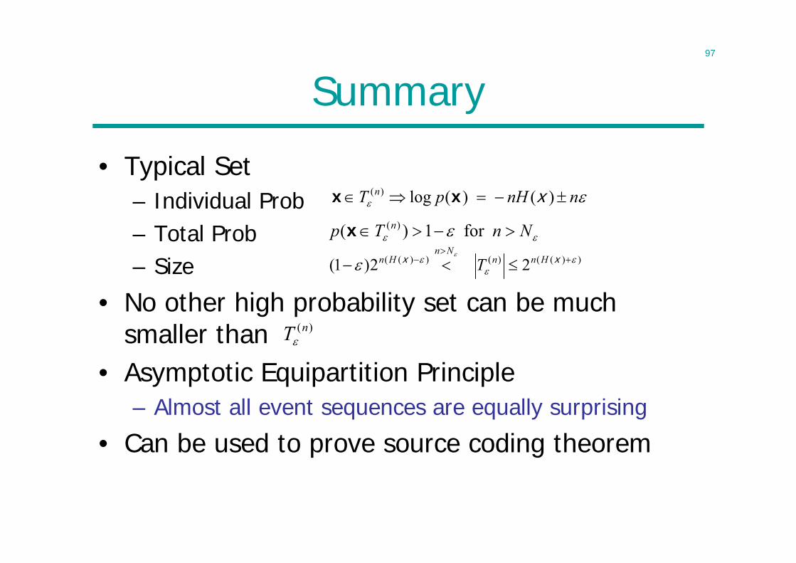
• Typical Set– Individual Prob– Total Prob– Size
• No other high probability set can be much smaller than
• Asymptotic Equipartition Principle– Almost all event sequences are equally surprising
• Can be used to prove source coding theorem
nnHpT n )()(log)( xxx
NnTp n for 1)( )(x
22)1( ))(()())((
xx HnnNn
Hn T
)(nT
98
Lecture 8
• Channel Coding• Channel Capacity
– The highest rate in bits per channel use that can be transmitted reliably
– The maximum mutual information• Discrete Memoryless Channels
– Symmetric Channels– Channel capacity
• Binary Symmetric Channel• Binary Erasure Channel• Asymmetric Channel
= proved in channel coding theorem
99
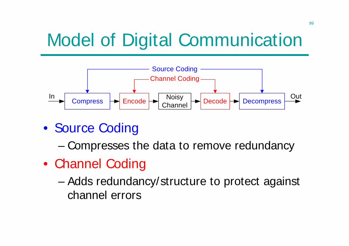
Model of Digital Communication
• Source Coding– Compresses the data to remove redundancy
• Channel Coding– Adds redundancy/structure to protect against
channel errors
Compress DecompressEncode DecodeNoisyChannel
Source CodingChannel Coding
In Out
100
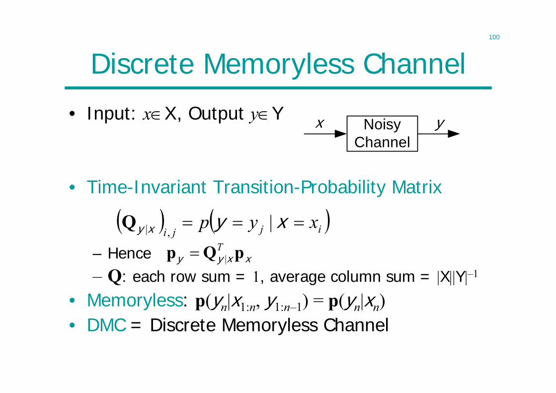
Discrete Memoryless Channel
• Input: xX, Output yY
• Time-Invariant Transition-Probability Matrix
– Hence– Q: each row sum = 1, average column sum = |X||Y|–1
• Memoryless: p(yn|x1:n, y1:n–1) = p(yn|xn)• DMC = Discrete Memoryless Channel
ijjixyp xyxy |
,|Q
xxyy pQp T|
NoisyChannel
x y
101
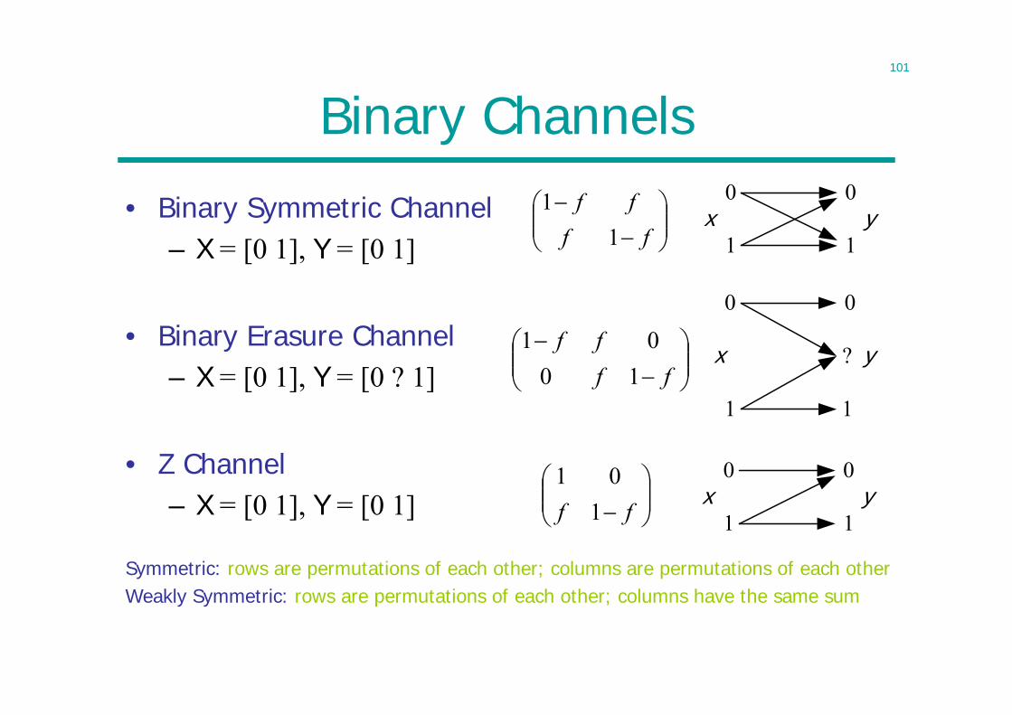
Binary Channels
• Binary Symmetric Channel– X = [0 1], Y = [0 1]
• Binary Erasure Channel– X = [0 1], Y = [0 ? 1]
• Z Channel– X = [0 1], Y = [0 1]
Symmetric: rows are permutations of each other; columns are permutations of each otherWeakly Symmetric: rows are permutations of each other; columns have the same sum
ff
ff1
1
ff
ff10
01
ff 101
x0
1
0
1y
x0
1
0
1y
x
0
1
0
? y
1
102
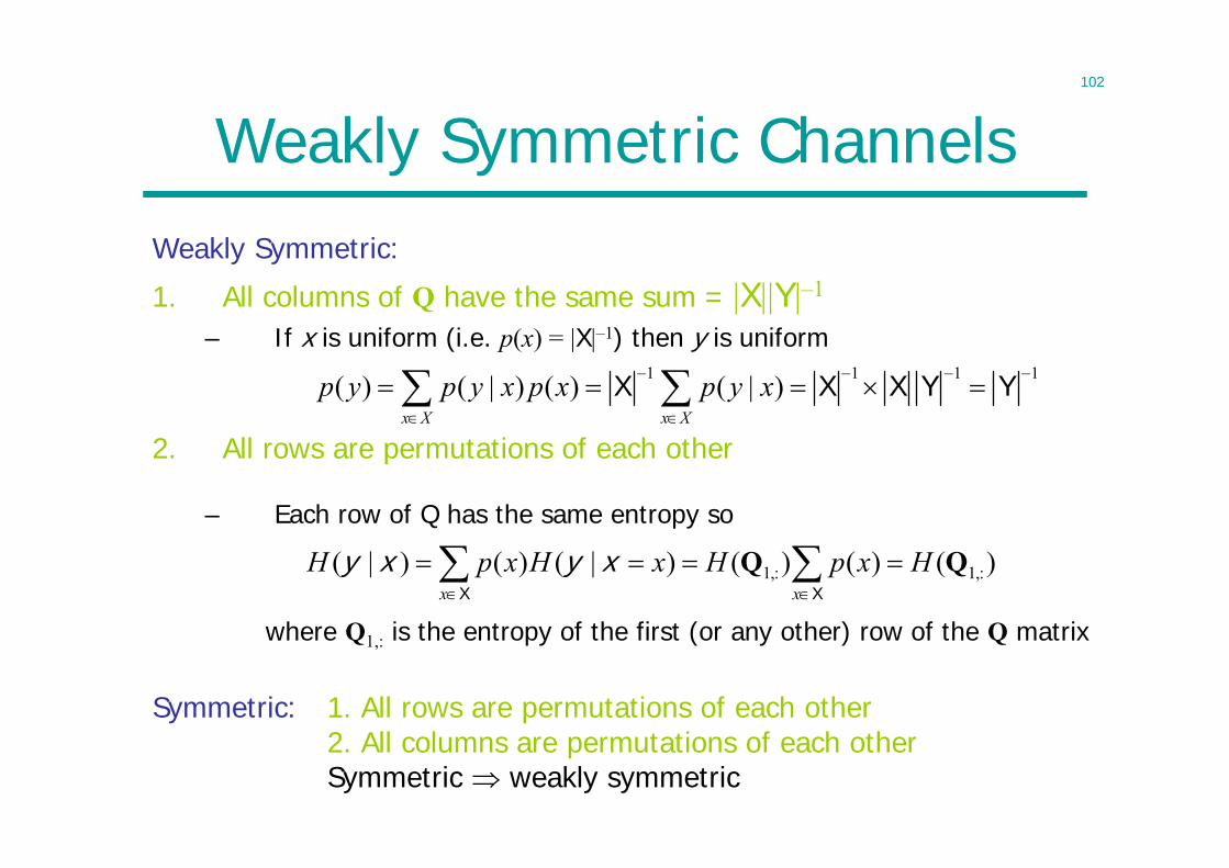
Weakly Symmetric ChannelsWeakly Symmetric:
1. All columns of Q have the same sum = |X||Y|–1
– If x is uniform (i.e. p(x) = |X|–1) then y is uniform1 1 1 1( ) ( | ) ( ) ( | )
x X x Xp y p y x p x p y x
X X X Y Y
)()()()|()()|( :,1:,1 QQ HxpHxHxpHxx
XX
xyxy
where Q1,: is the entropy of the first (or any other) row of the Q matrix
Symmetric: 1. All rows are permutations of each other2. All columns are permutations of each otherSymmetric weakly symmetric
2. All rows are permutations of each other
– Each row of Q has the same entropy so
103
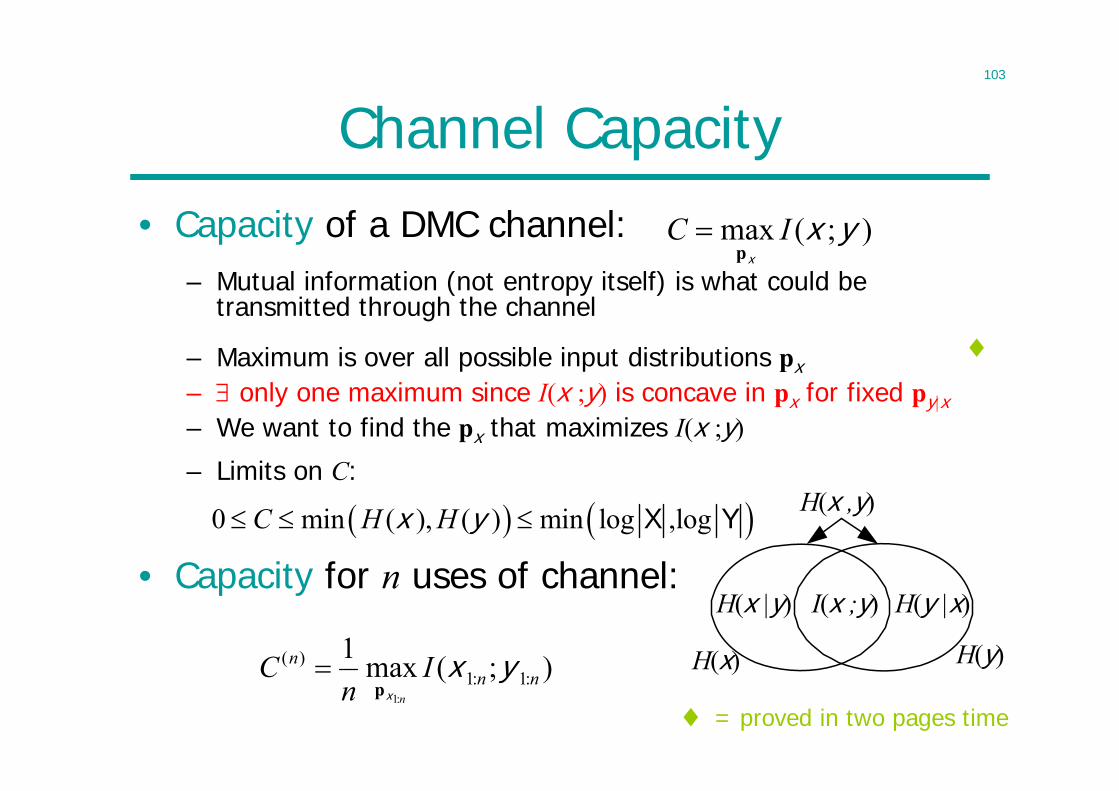
Channel Capacity• Capacity of a DMC channel:
– Mutual information (not entropy itself) is what could be transmitted through the channel
– Maximum is over all possible input distributions px– only one maximum since I(x ;y) is concave in px for fixed py|x– We want to find the px that maximizes I(x ;y)
);(max yxx
ICp
);(max1:1:1
)(
:1nn
n In
Cn
yxxp
0 min ( ), ( ) min log ,logC H H x y X Y
= proved in two pages time
H(x |y) H(y |x)
H(x ,y)
H(x) H(y)
I(x ;y)• Capacity for n uses of channel:
– Limits on C:
104
00.2
0.40.6
0.81 0
0.20.4
0.60.8
1-0.5
0
0.5
1
Channel Error Prob (f)
I(X;Y)
Input Bernoulli Prob (p)
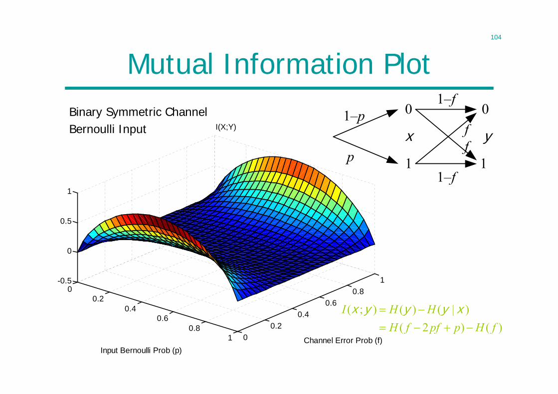
Mutual Information PlotBinary Symmetric ChannelBernoulli Input f
0
1
0
1
yxf
1–f
1–f
1–p
p
( ; ) ( ) ( | )( 2 ) ( )
I H HH f pf p H f
x y y y x
105
Mutual Information Concave in pX
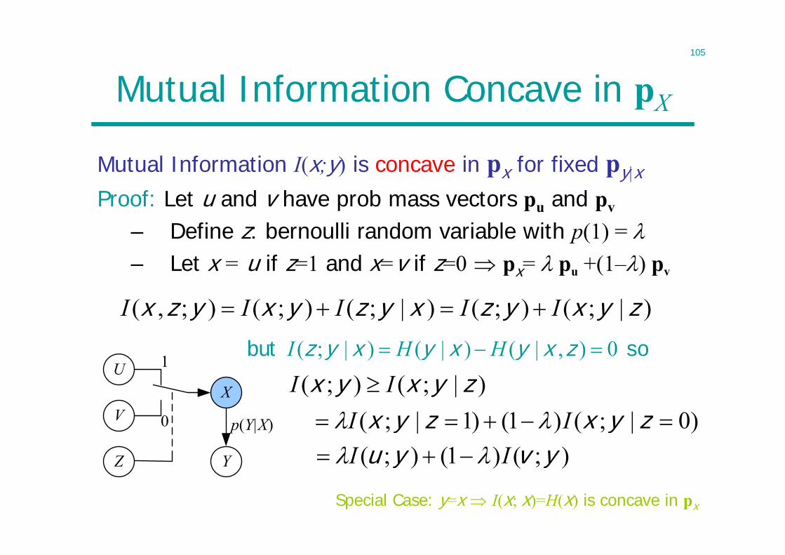
Mutual Information I(x;y) is concave in px for fixed py|x
)|;();()|;();();,( zyxyzxyzyxyzx IIIII
U
VX
Z Y
p(Y|X)
1
0
sobut 0),|()|()|;( zxyxyxyz HHI
);()1();( yvyu II
Special Case: y=x I(x; x)=H(x) is concave in px
)|;();( zyxyx II )0|;()1()1|;( zyxzyx II
Proof: Let u and v have prob mass vectors pu and pv
– Define z: bernoulli random variable with p(1) = – Let x = u if z=1 and x=v if z=0 px= pu +(1–) pv
106
Mutual Information Convex in pY|X
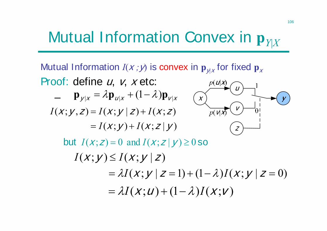
Mutual Information I(x ;y) is convex in py|x for fixed px
xvxuxy ||| )1( ppp
)|;();();()|;(),;(
yzxyxzxzyxzyx
IIIII
sobut 0)|;( and 0);( yzxzx II)|;();( zyxyx II
Proof: define u, v, x etc:–
)0|;()1()1|;( zyxzyx II );()1();( vxux II
107
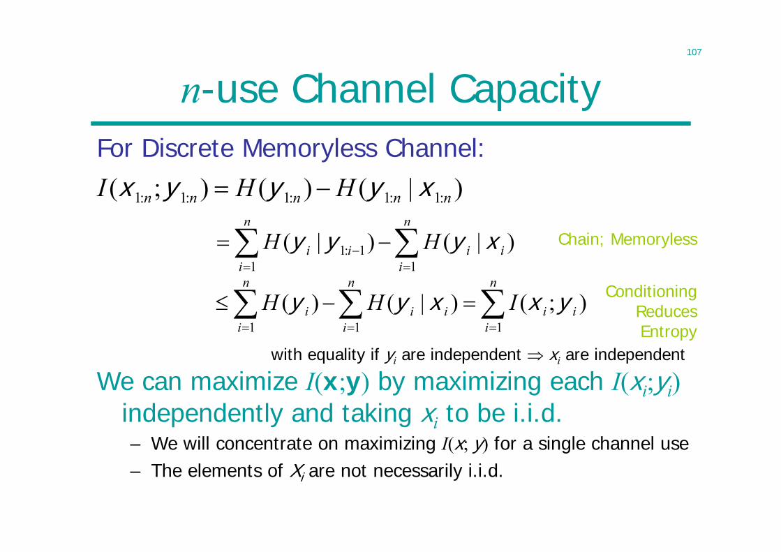
n-use Channel Capacity
We can maximize I(x;y) by maximizing each I(xi;yi)independently and taking xi to be i.i.d.– We will concentrate on maximizing I(x; y) for a single channel use– The elements of Xi are not necessarily i.i.d.
)|()();( :1:1:1:1:1 nnnnn HHI xyyyx For Discrete Memoryless Channel:
with equality if yi are independent xi are independent
Chain; Memoryless
ConditioningReducesEntropy
n
iii
n
iii
n
ii IHH
111);()|()( yxxyy
n
iii
n
iii HH
111:1 )|()|( xyyy
108
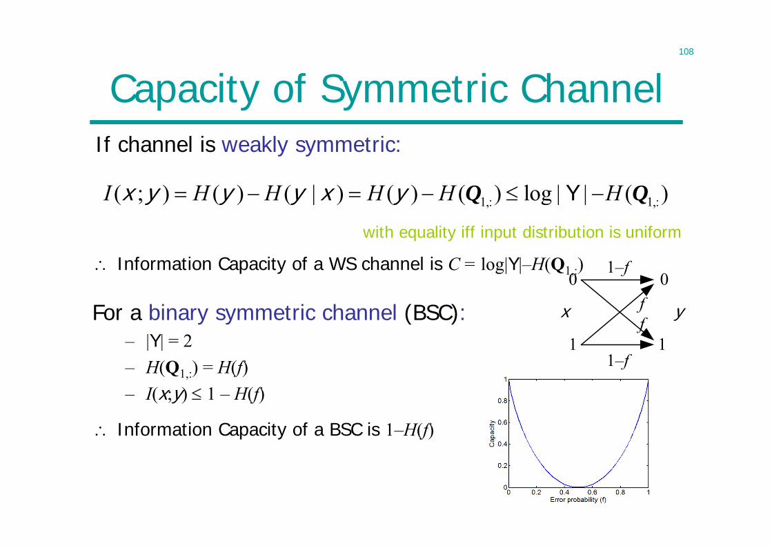
Capacity of Symmetric Channel
Information Capacity of a BSC is 1–H(f)
f0
1
0
1
yxf
1–f
1–f
1,: 1,:( ; ) ( ) ( | ) ( ) ( ) log | | ( )I H H H H H x y y y x y YQ Q
with equality iff input distribution is uniform
If channel is weakly symmetric:
For a binary symmetric channel (BSC):– |Y| = 2– H(Q1,:) = H(f)– I(x;y) 1 – H(f)
Information Capacity of a WS channel is C = log|Y|–H(Q1,:)
109
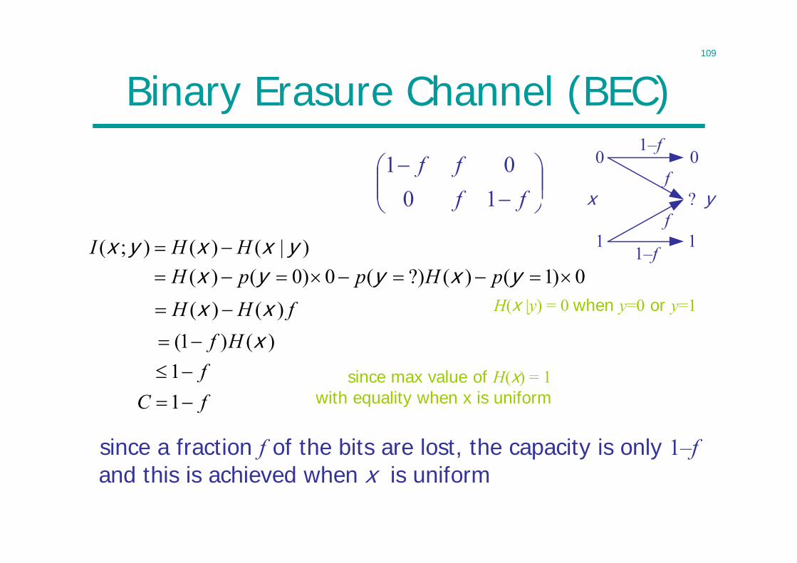
Binary Erasure Channel (BEC)
since a fraction f of the bits are lost, the capacity is only 1–fand this is achieved when x is uniform
x
0
1
0
? y
1
f
f
1–f
1–f)|()();( yxxyx HHI
ff
ff10
01
since max value of H(x) = 1with equality when x is uniform
H(x |y) = 0 when y=0 or y=1fHH )()( xx
0)1()(?)(0)0()( yxyyx pHppH
11
fC f
)()1( xHf
110
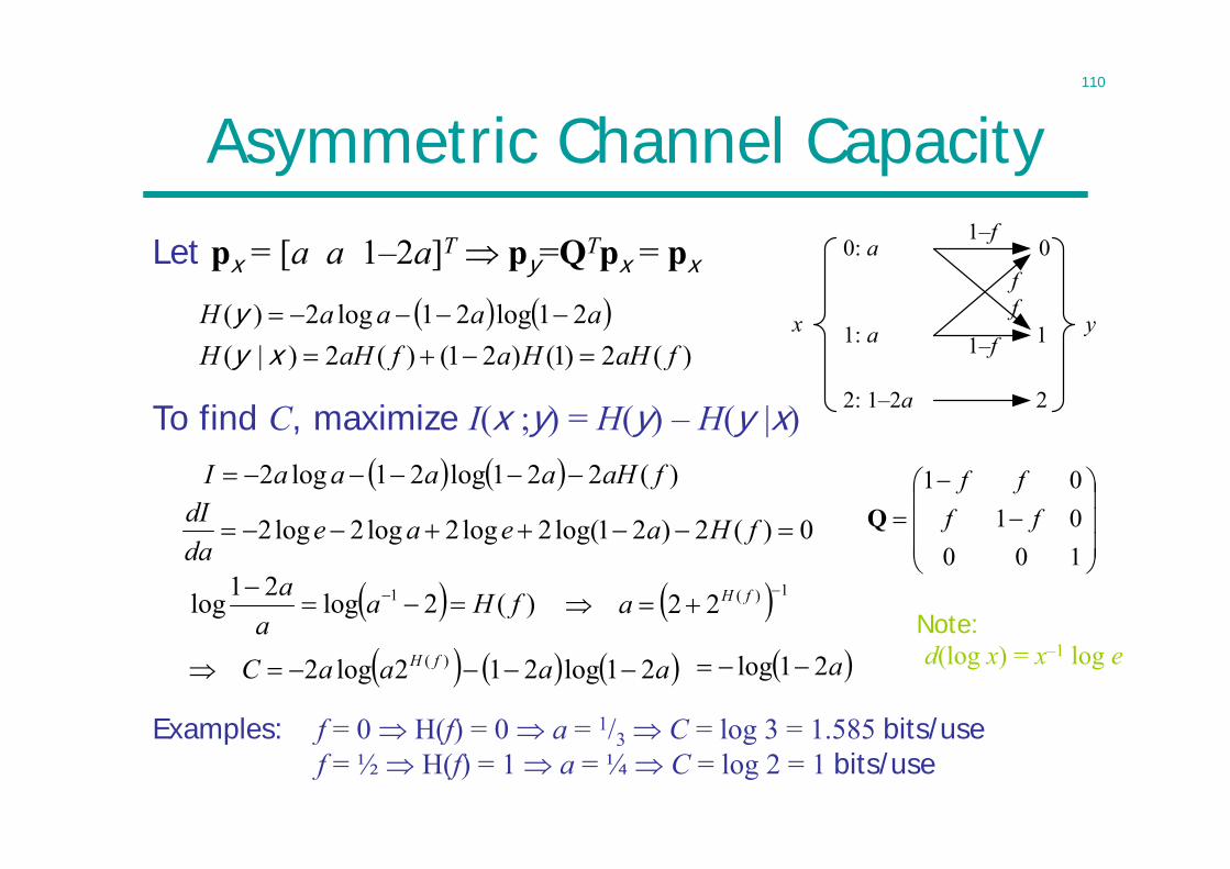
Asymmetric Channel Capacity
Let px = [a a 1–2a]T py=QTpx = pxf
0: a
1: a
0
1 yxf
1–f
1–f
2: 1–2a 2
1000101
ffff
Q
To find C, maximize I(x ;y) = H(y) – H(y |x) )(221log21log2 faHaaaaI
Note:d(log x) = x–1 log e
Examples: f = 0 H(f) = 0 a = 1/3 C = log 3 = 1.585 bits/usef = ½ H(f) = 1 a = ¼ C = log 2 = 1 bits/use
)(2)1()21()(2)|(
21log21log2)(faHHafaHH
aaaaH
xy
y
aaaaC fH 21log212log2 )(
0)(2)21log(2log2log2log2 fHaeaedadI
)(2log21log 1 fHaa
a
1)(22 fHa
a21log
111
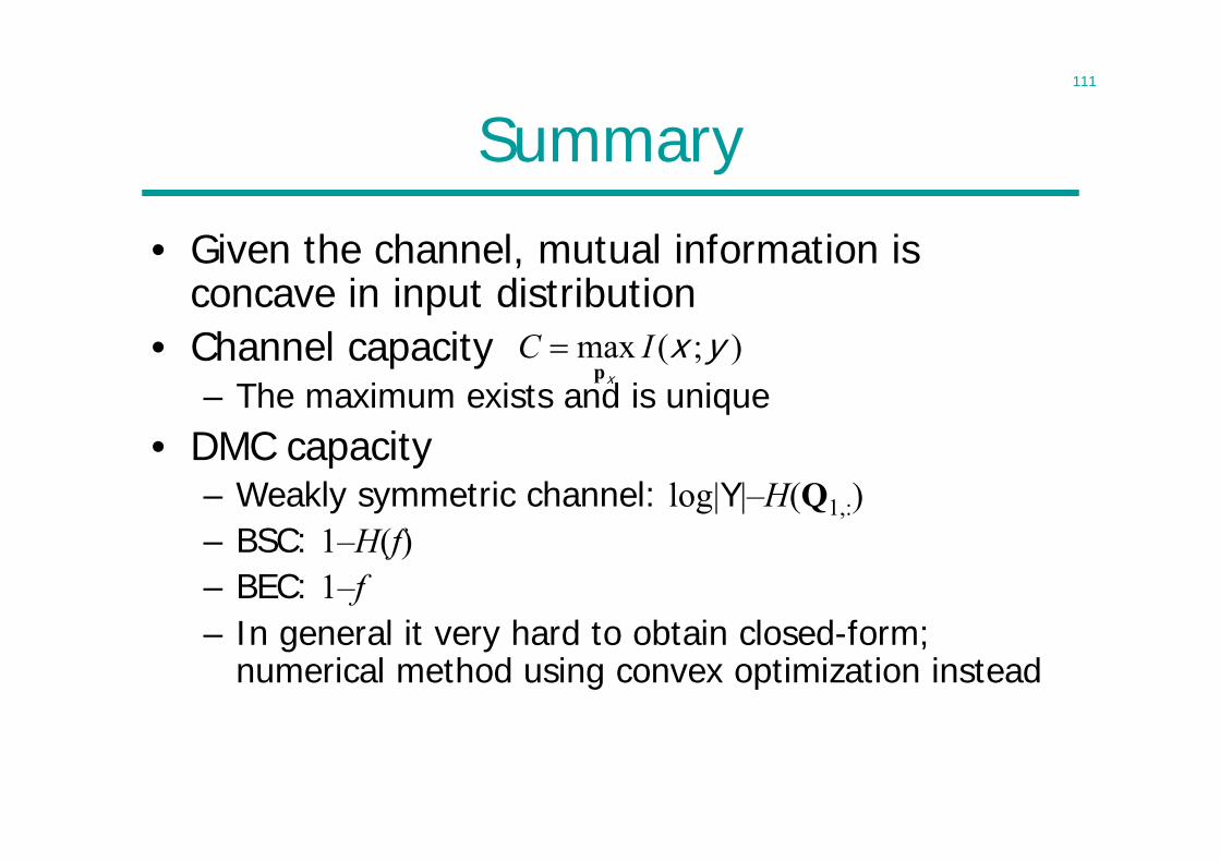
Summary
• Given the channel, mutual information is concave in input distribution
• Channel capacity – The maximum exists and is unique
• DMC capacity– Weakly symmetric channel: log|Y|–H(Q1,:)– BSC: 1–H(f)– BEC: 1–f– In general it very hard to obtain closed-form;
numerical method using convex optimization instead
);(max yxx
ICp
112
Lecture 9
• Jointly Typical Sets• Joint AEP• Channel Coding Theorem
– Ultimate limit on information transmission is channel capacity
– The central and most successful story of information theory
– Random Coding– Jointly typical decoding
113
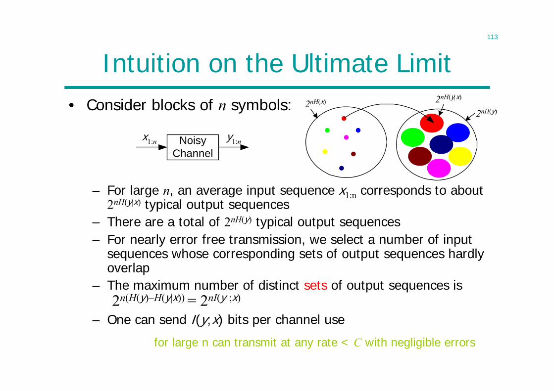
Intuition on the Ultimate Limit
– For large n, an average input sequence x1:n corresponds to about 2nH(y|x) typical output sequences
– There are a total of 2nH(y) typical output sequences– For nearly error free transmission, we select a number of input
sequences whose corresponding sets of output sequences hardly overlap
– The maximum number of distinct sets of output sequences is2n(H(y)–H(y|x)) = 2nI(y ;x)
– One can send I(y;x) bits per channel use
NoisyChannel
x1:n y1:n
2nH(x) 2nH(y|x)
2nH(y)• Consider blocks of n symbols:
for large n can transmit at any rate < C with negligible errors
114
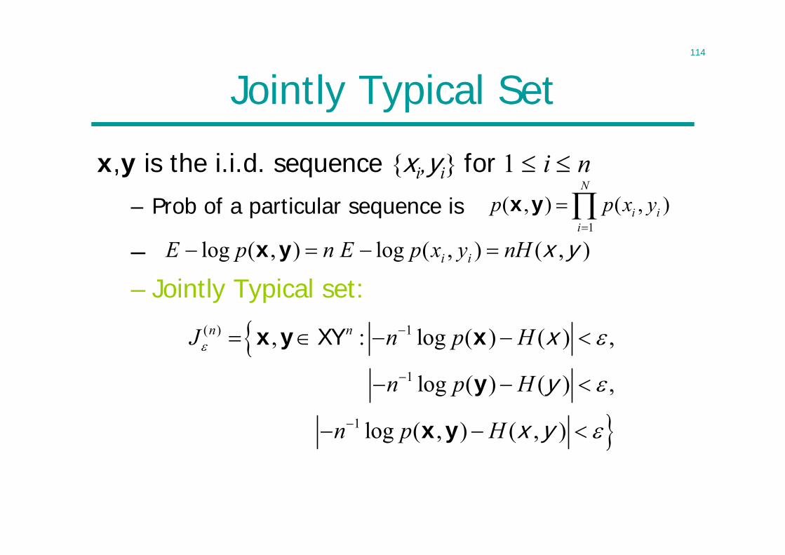
Jointly Typical Set
x,y is the i.i.d. sequence {xi,yi} for 1 i n– Prob of a particular sequence is
–– Jointly Typical set:
1
( , ) ( , )N
i ii
p p x y
x y
),(),(log),(log yxnHyxpEnpE ii yx
( ) 1
1
1
, : log ( ) ( ) ,
log ( ) ( ) ,
log ( , ) ( , )
n nJ n p H
n p H
n p H
x
y
x y
XYx y x
y
x y
115
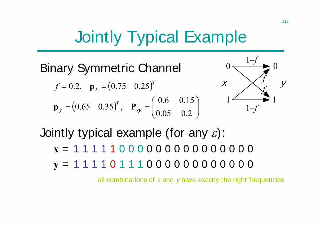
Jointly Typical Example
Binary Symmetric Channelf
0
1
0
1
yxf
1–f
1–f
2.005.015.06.0
,35.065.0
25.075.0,2.0
xyy
x
Pp
p
T
Tf
Jointly typical example (for any ):x = 1 1 1 1 1 0 0 0 0 0 0 0 0 0 0 0 0 0 0 0y = 1 1 1 1 0 1 1 1 0 0 0 0 0 0 0 0 0 0 0 0
all combinations of x and y have exactly the right frequencies
116
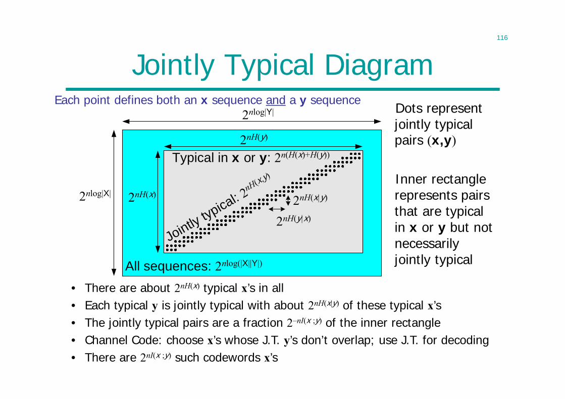
Jointly Typical DiagramDots represent jointly typical pairs (x,y)
Inner rectangle represents pairs that are typical in x or y but not necessarily jointly typical
2nlog|X| 2nH(x)
2nlog|Y|
2nH(y)
2nH(y|x)
2nH(x|y)
Typical in x or y: 2n(H(x)+H(y))
All sequences: 2nlog(|X||Y|)
Jointly typical: 2nH(x,y)
• There are about 2nH(x) typical x’s in all• Each typical y is jointly typical with about 2nH(x|y) of these typical x’s• The jointly typical pairs are a fraction 2–nI(x ;y) of the inner rectangle • Channel Code: choose x’s whose J.T. y’s don’t overlap; use J.T. for decoding• There are 2nI(x ;y) such codewords x’s
Each point defines both an x sequence and a y sequence
117
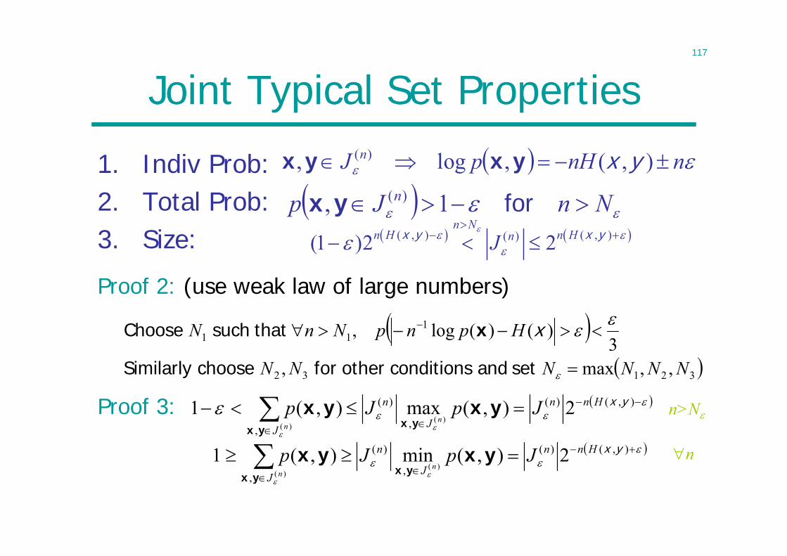
Joint Typical Set Properties
1. Indiv Prob:2. Total Prob: 3. Size:
NnJp n for1, )(yx ( , ) ( , )( )(1 )2 2
n Nn H n HnJ
x y x y
Proof 2: (use weak law of large numbers)
32132
111
,,max,3
)()(log,
NNNNNN
HpnpNnN
set and conditionsother for chooseSimilarly
that such Choose xx
nnHpJ n ),(,log, )( yxyxyx
),()(
,
)(
,
2),(max),(1)(
)(
yxHnn
J
n
J
JpJpn
n
yxyxyxyx
n
n>NProof 3:
),()(
,
)(
,
2),(min),(1)(
)(
yxHnn
J
n
J
JpJpn
n
yxyxyxyx
118
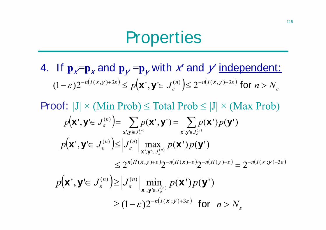
Properties
4. If px'=px and py' =py with x' and y' independent:
NnJp InnIn for 3),()(3),( 2','2)1( yxyx yx
Proof: |J| × (Min Prob) Total Prob |J| × (Max Prob)
Nn
ppJJp
In
J
nnn
for 3);(
','
)()(
2)1(
)'()'(min',')(
y x
yxyxyx
)()( ','','
)( )'()'()','(','nn JJ
n pppJp
yxyx
yxyxyx
3);()()(),(
','
)()(
2222
)'()'(max',')(
y xyxyx InHnHnHn
J
nn ppJJpn
yxyxyx
119
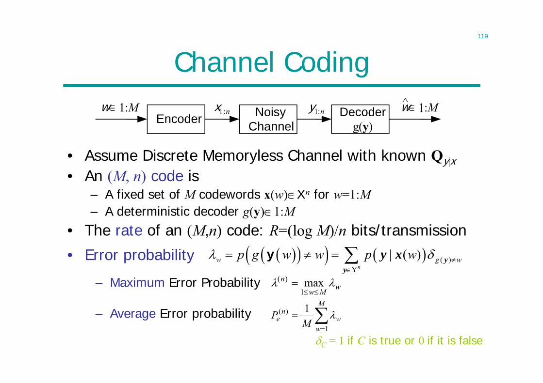
Channel Coding
• Assume Discrete Memoryless Channel with known Qy|x• An (M, n) code is
– A fixed set of M codewords x(w)Xn for w=1:M– A deterministic decoder g(y)1:M
• The rate of an (M,n) code: R=(log M)/n bits/transmission
NoisyChannel
x1:n y1:nEncoder
w1:M Decoderg(y)
w1:M^
( )Y
| ( )n
w g wp g w w p w
yy
y xy
M
ww
ne M
P1
)( 1
C = 1 if C is true or 0 if it is false
• Error probability
– Maximum Error Probability
– Average Error probability
wMw
n
1
)( max
120
Shannon’s ideas• Channel coding theorem: the basic theorem of
information theory– Proved in his original 1948 paper
• How do you correct all errors?• Shannon’s ideas
– Allowing arbitrarily small but nonzero error probability– Using the channel many times in succession so that
AEP holds– Consider a randomly chosen code and show the
expected average error probability is small• Use the idea of typical sequences• Show this means at least one code with small max error
prob• Sadly it doesn’t tell you how to construct the code
121
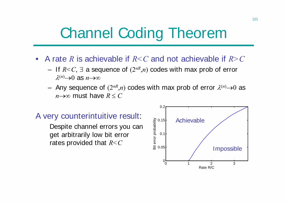
Channel Coding Theorem
• A rate R is achievable if R<C and not achievable if R>C– If R<C, a sequence of (2nR,n) codes with max prob of error
(n)0 as n– Any sequence of (2nR,n) codes with max prob of error (n)0 as
n must have R C
0 1 2 30
0.05
0.1
0.15
0.2
Rate R/C
Bit
erro
r pro
babi
lity Achievable
Impossible
A very counterintuitive result:Despite channel errors you can get arbitrarily low bit error rates provided that R<C
122
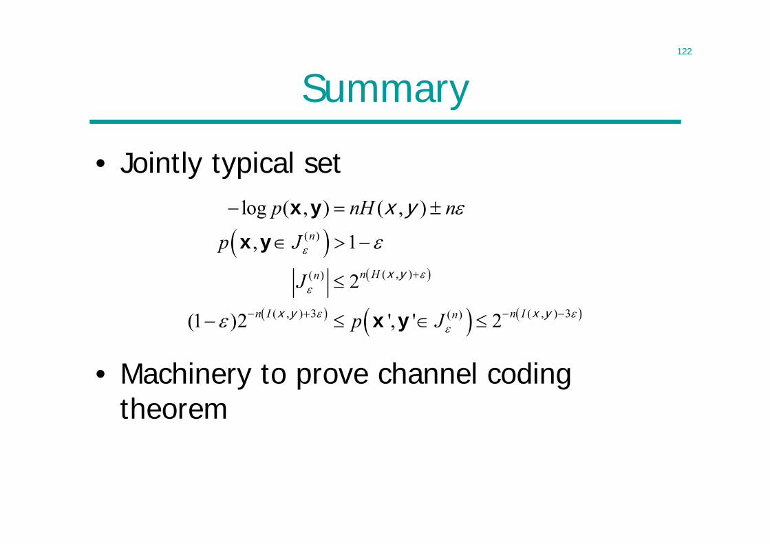
Summary
• Jointly typical set
• Machinery to prove channel coding theorem
( )
( , )( )
( , ) 3 ( , ) 3( )
log ( , ) ( , )
, 1
2
(1 )2 ', ' 2
n
n Hn
n I n In
p nH n
p J
J
p J
x y
x y x y
x yx y
x y
x y
123
Lecture 10
• Channel Coding Theorem– Proof
• Using joint typicality• Arguably the simplest one among many possible
ways• Limitation: does not reveal Pe ~ e-nE(R)
– Converse (next lecture)
124
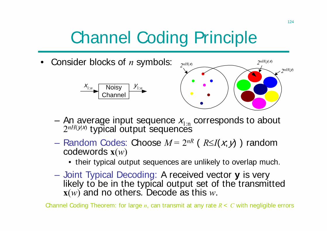
Channel Coding Principle
– An average input sequence x1:n corresponds to about 2nH(y|x) typical output sequences
NoisyChannel
x1:n y1:n
2nH(x) 2nH(y|x)
2nH(y)• Consider blocks of n symbols:
Channel Coding Theorem: for large n, can transmit at any rate R < C with negligible errors
– Random Codes: Choose M = 2nR ( RI(x;y) ) random codewords x(w)
• their typical output sequences are unlikely to overlap much.
– Joint Typical Decoding: A received vector y is very likely to be in the typical output set of the transmitted x(w) and no others. Decode as this w.
125
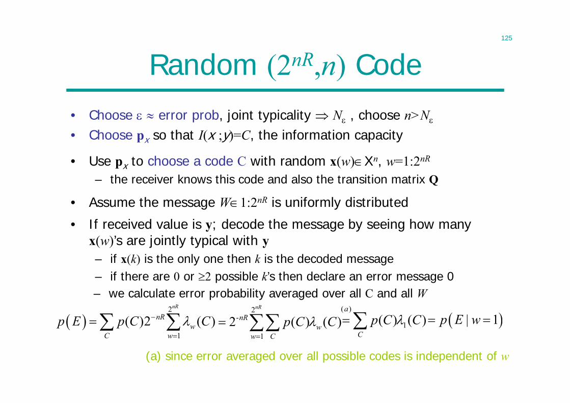
Random (2nR,n) Code• Choose error prob, joint typicality N , choose n>N
2
1( )2 ( )
nR
nRw
C wp E p C C
(a) since error averaged over all possible codes is independent of w
• Choose px so that I(x ;y)=C, the information capacity
• Use px to choose a code C with random x(w)Xn, w=1:2nR
– the receiver knows this code and also the transition matrix Q
• Assume the message W1:2nR is uniformly distributed
• If received value is y; decode the message by seeing how many x(w)’s are jointly typical with y– if x(k) is the only one then k is the decoded message– if there are 0 or 2 possible k’s then declare an error message 0– we calculate error probability averaged over all C and all W
2-
12 ( ) ( )
nR
nRw
w Cp C C
( )
1( ) ( )a
Cp C C | 1p E w
126
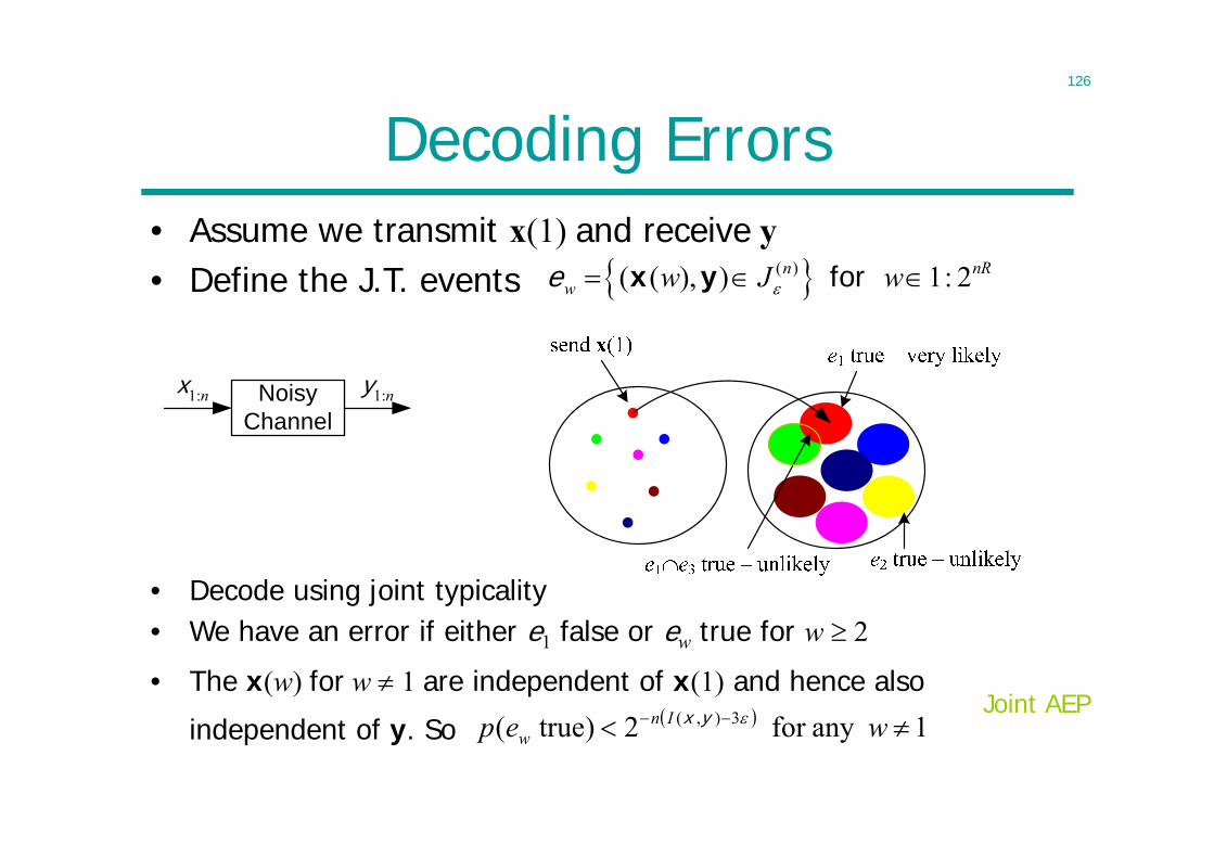
Decoding Errors
( )( ( ), ) 1: 2n nRw w J w for e x y
NoisyChannel
x1:n y1:n
• Assume we transmit x(1) and receive y• Define the J.T. events
• Decode using joint typicality • We have an error if either e1 false or ew true for w 2
• The x(w) for w 1 are independent of x(1) and hence also
independent of y. So 1any for 2) true( 3),( wep Inw
yx Joint AEP
127
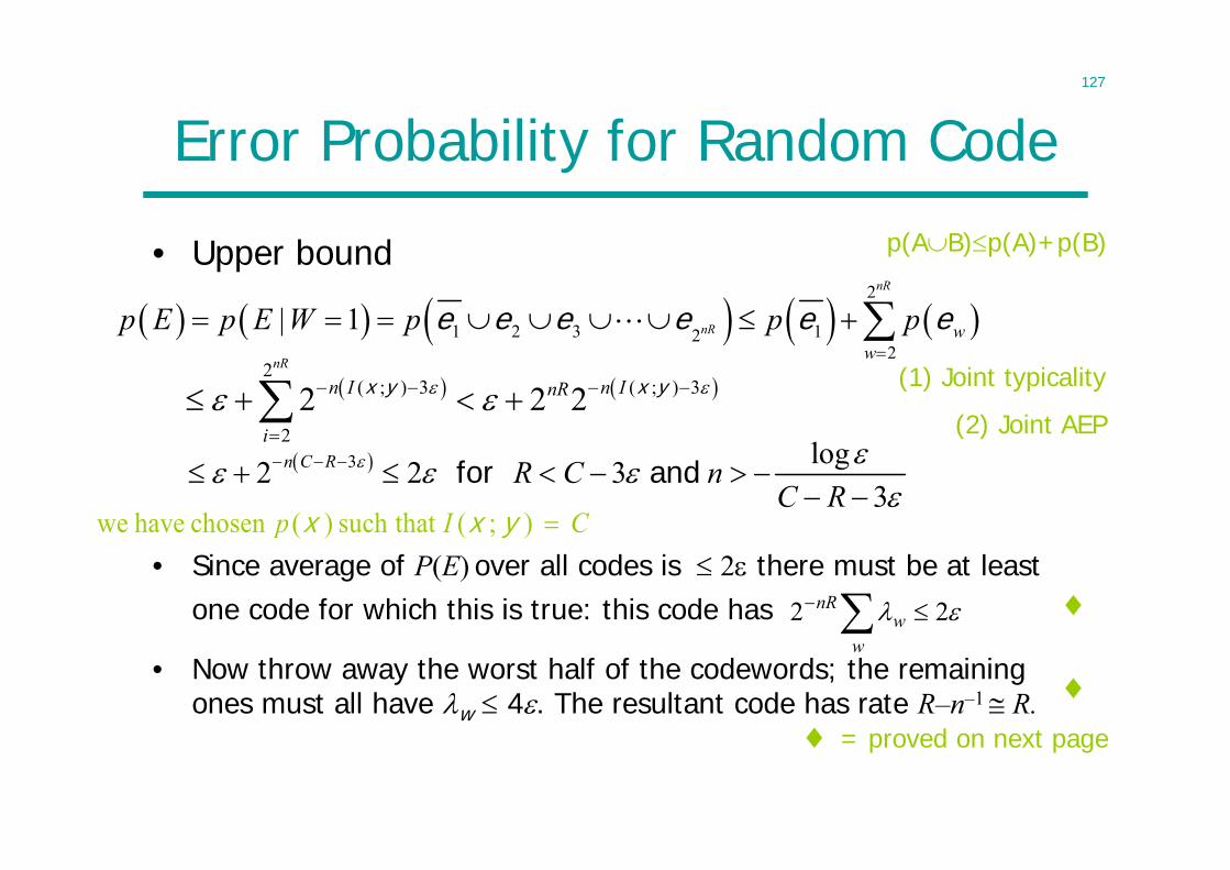
Error Probability for Random Code
2
1 2 3 122
| 1nR
nR ww
p E p E W p p p
e e e e e e
• Since average of P(E) over all codes is 2 there must be at least one code for which this is true: this code has 22
ww
nR
• Now throw away the worst half of the codewords; the remaining ones must all have w 4. The resultant code has rate R–n–1 R.
= proved on next page
(1) Joint typicality
(2) Joint AEP
p(AB)p(A)+p(B)
2
( ; ) 3 ( ; ) 3
2
2 2 2nR
n I n InR
i
x y x y
3 log2 2 33
n C R R C nC R
for and
• Upper bound
we have chosen ( ) such that ( ; )p I Cx x y
128
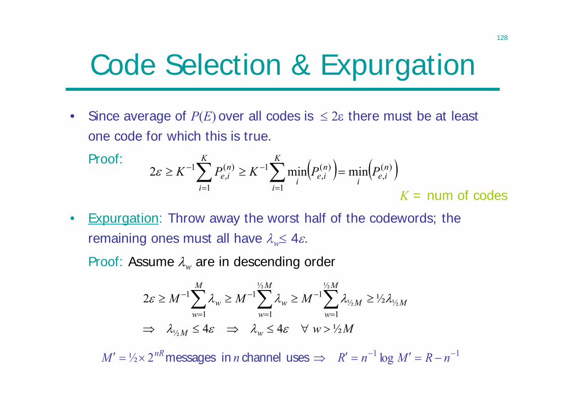
Code Selection & Expurgation• Since average of P(E) over all codes is 2 there must be at least
one code for which this is true.
Mw
MMM
wM
M
M
wM
M
ww
M
ww
½44
½2
½
½
½
1½
1½
1
1
1
1
)(,
1
)(,
1
1
)(,
1 minmin2 niei
K
i
niei
K
i
nie PPKPK
11 log 2½ nRMnRnM nR uses channelin messages
K = num of codes
Proof:
• Expurgation: Throw away the worst half of the codewords; the remaining ones must all have w 4.
Proof: Assume w are in descending order
129
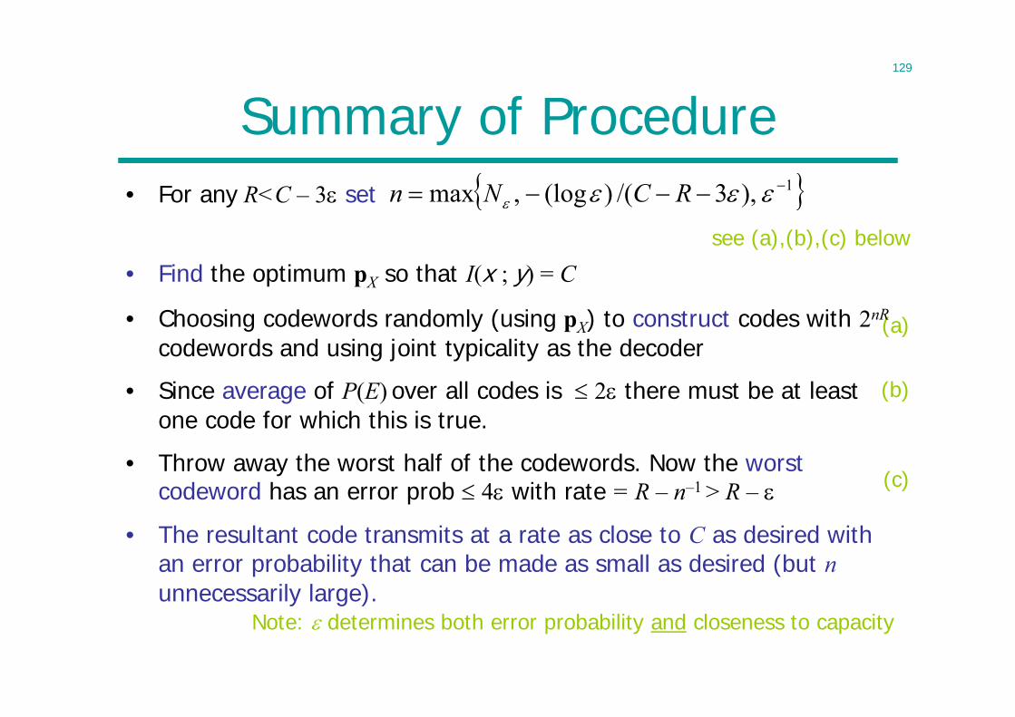
Summary of Procedure 1),3/()(log,max RCNn
see (a),(b),(c) below
(a)
(b)
(c)
Note: determines both error probability and closeness to capacity
• For any R<C – 3 set
• Find the optimum pX so that I(x ; y) = C
• Choosing codewords randomly (using pX) to construct codes with 2nR
codewords and using joint typicality as the decoder
• Since average of P(E) over all codes is 2 there must be at least one code for which this is true.
• Throw away the worst half of the codewords. Now the worst codeword has an error prob 4 with rate = R – n–1 > R –
• The resultant code transmits at a rate as close to C as desired with an error probability that can be made as small as desired (but nunnecessarily large).
130
Remarks• Random coding is a powerful method of proof,
not a method of signaling• Picking randomly will give a good code• But n has to be large (AEP)• Without a structure, it is difficult to
encode/decode– Table lookup requires exponential size
• Channel coding theorem does not provide a practical coding scheme
• Folk theorem (but outdated now):– Almost all codes are good, except those we can think
of
131
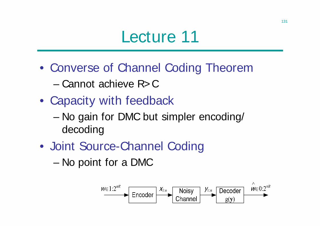
Lecture 11
• Converse of Channel Coding Theorem– Cannot achieve R>C
• Capacity with feedback– No gain for DMC but simpler encoding/
decoding
• Joint Source-Channel Coding– No point for a DMC
132
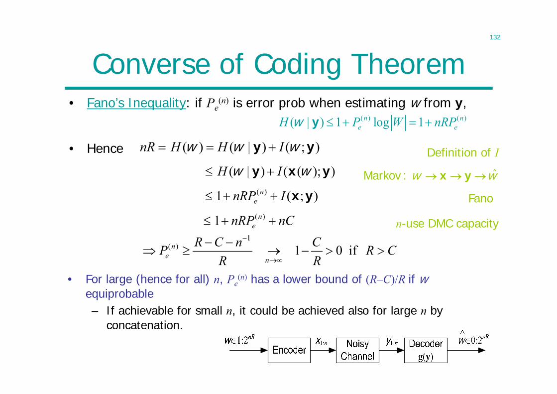
Converse of Coding Theorem• Fano’s Inequality: if Pe
(n) is error prob when estimating w from y,( ) ( )( | ) 1 log 1n n
e eH P W nRP w y
• Hence );()|()( yy www IHHnR
• For large (hence for all) n, Pe(n) has a lower bound of (R–C)/R if w
equiprobable– If achievable for small n, it could be achieved also for large n by
concatenation.
n-use DMC capacity
Fano
ww ˆ yx :Markov
Definition of I));(()|( yxy ww IH
);(1 )( yxInRP ne
nCnRP ne )(1
1( ) 1 0 ifn
e n
R C n CP R CR R
133
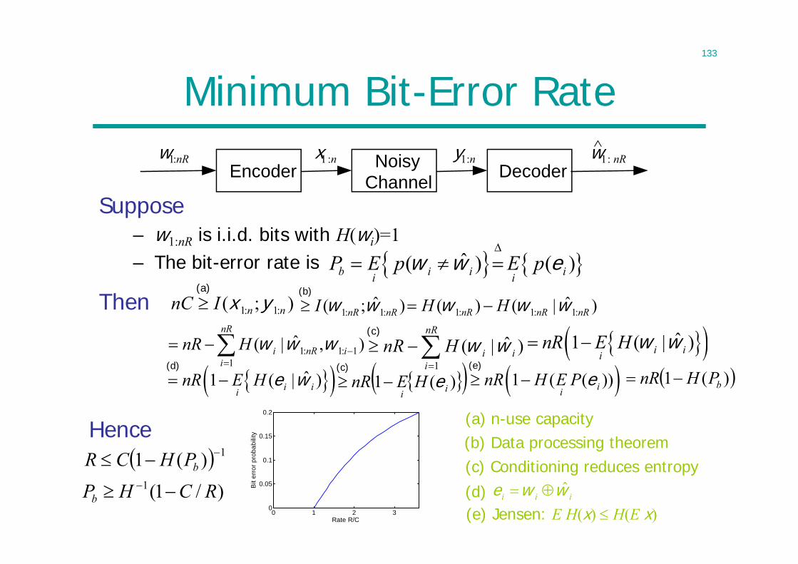
Minimum Bit-Error Rate
Suppose– w1:nR is i.i.d. bits with H(wi)=1– The bit-error rate is
^Noisy
Channelx1:n y1:n
Encoderw1:nR
Decoderw1: nR
ˆ( ) ( )b i i ii iP E p E p
w w e
);( :1:1 nnInC yx(a)
Hence 1)(1 bPHCR
(a) n-use capacity
0 1 2 30
0.05
0.1
0.15
0.2
Rate R/C
Bit
erro
r pro
babi
lity
ˆi i i e w w
1: 1:ˆ( ; )nR nRI w w
(b)
1: 1: 1:ˆ( ) ( | )nR nR nRH H w w w
1: 1: 11
ˆ( | , )nR
i nR ii
nR H
w w w1
ˆ( | )nR
i ii
nR H
w w(c) ˆ1 ( | )i ii
nR E H w w
ˆ1 ( | )i iinR E H e w
(d)
)(1 iiHEnR e
(c) )(1 bPHnR
(b) Data processing theorem(c) Conditioning reduces entropy(d)
Then
)/1(1 RCHPb
1 ( ( ))iinR H E P e
(e)
(e) Jensen: E H(x) H(E x)
134
Coding Theory and Practice• Construction for good codes
– Ever since Shannon founded information theory– Practical: Computation & memory nk for some k
• Repetition code: rate 0• Block codes: encode a block at a time
– Hamming code: correct one error– Reed-Solomon code, BCH code: multiple errors (1950s)
• Convolutional code: convolve bit stream with a filter• Concatenated code: RS + convolutional• Capacity-approaching codes:
– Turbo code: combination of two interleaved convolutional codes (1993)
– Low-density parity-check (LDPC) code (1960)– Dream has come true for some channels today
135
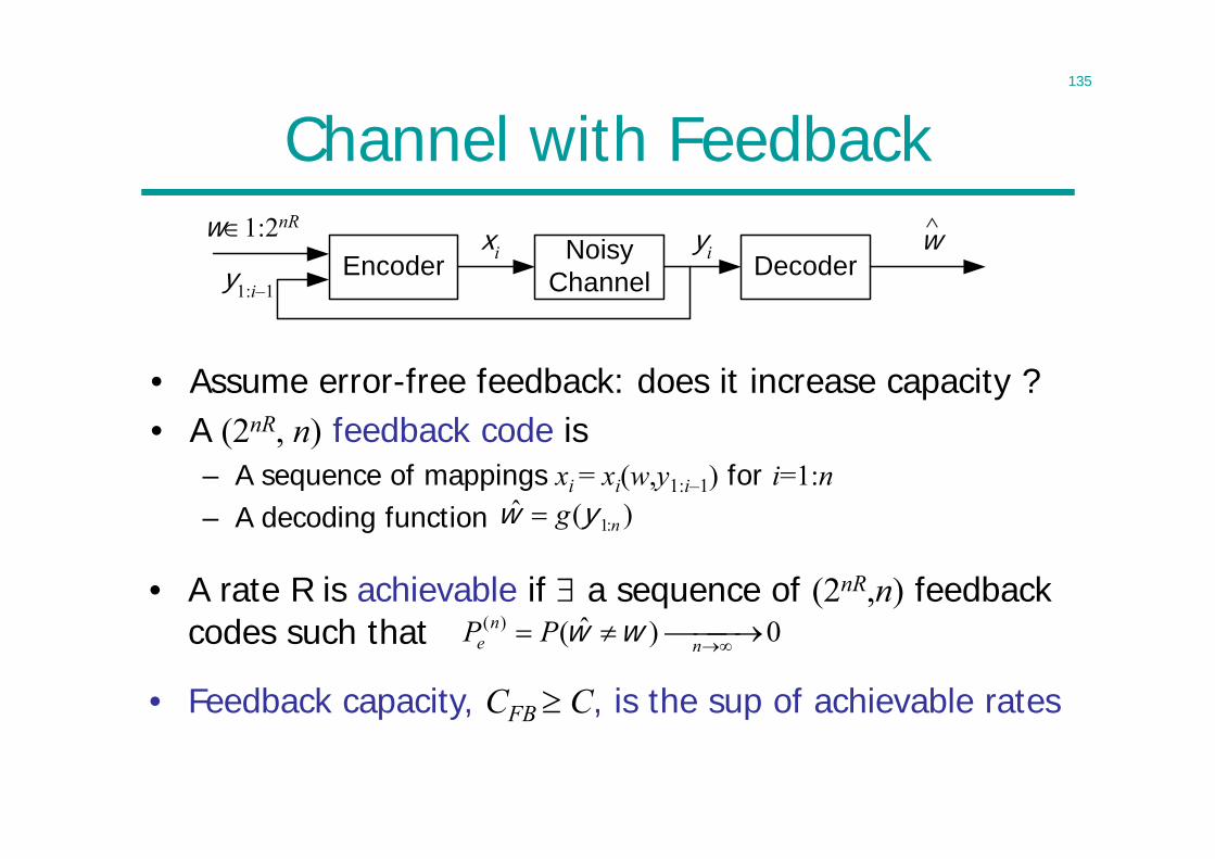
Channel with Feedback
• Assume error-free feedback: does it increase capacity ?• A (2nR, n) feedback code is
– A sequence of mappings xi = xi(w,y1:i–1) for i=1:n– A decoding function
NoisyChannel
xi yiEncoderw1:2nR
Decoderw
y1:i–1
)(ˆ :1 ng yw
0)ˆ()( nn
e PP ww• A rate R is achievable if a sequence of (2nR,n) feedback
codes such that
• Feedback capacity, CFB C, is the sup of achievable rates
136
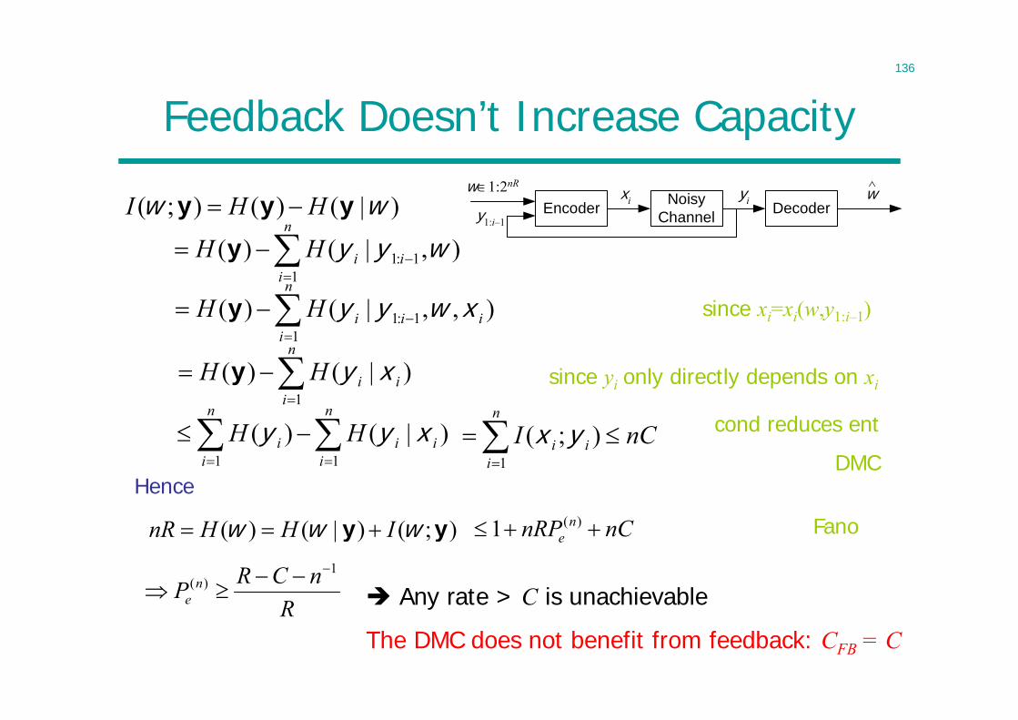
Feedback Doesn’t Increase Capacity
);()|()( yy www IHHnR
)|()();( ww yyy HHI
Hence
since xi=xi(w,y1:i–1)
since yi only directly depends on xi
Any rate > C is unachievable
The DMC does not benefit from feedback: CFB = C
cond reduces ent
DMC
Fano
NoisyChannel
xi yiEncoderw1:2nR
Decoderw
y1:i–1
n
iiiHH
11:1 ),|()( wyyy
n
iiiiHH
11:1 ),,|()( xwyyy
n
iiiHH
1)|()( xyy
n
iii
n
ii HH
11
)|()( xyy nCIn
iii
1
);( yx
nCnRP ne )(1
RnCRP n
e
1)(
137
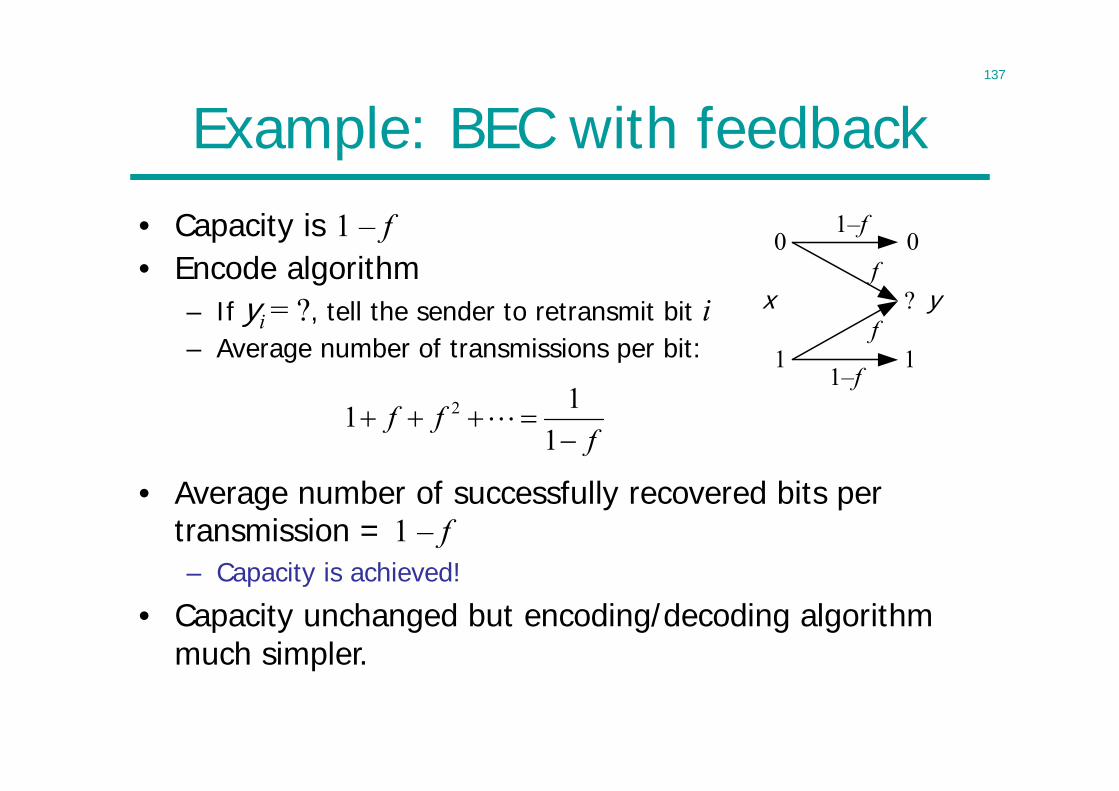
Example: BEC with feedback• Capacity is 1 – f• Encode algorithm
– If yi = ?, tell the sender to retransmit bit i– Average number of transmissions per bit:
x
0
1
0
? y
1
f
f
1–f
1–f
fff
111 2
• Average number of successfully recovered bits per transmission = 1 – f– Capacity is achieved!
• Capacity unchanged but encoding/decoding algorithm much simpler.
138
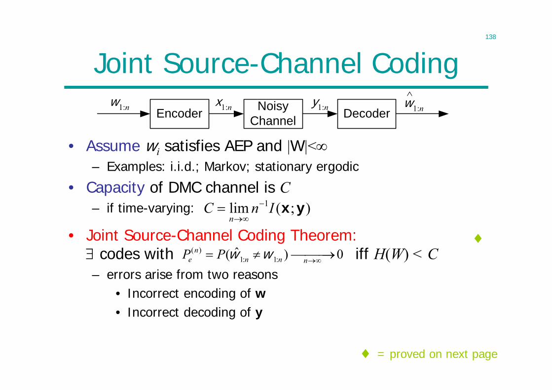
Joint Source-Channel Coding
• Assume wi satisfies AEP and |W|<– Examples: i.i.d.; Markov; stationary ergodic
• Capacity of DMC channel is C– if time-varying:
NoisyChannel
x1:n y1:nEncoderw1:n Decoder
w1:n
( )1: 1:
ˆ( ) 0ne n n nP P w w
);(lim 1 yxInCn
= proved on next page
• Joint Source-Channel Coding Theorem: codes with iff H(W) < C– errors arise from two reasons
• Incorrect encoding of w• Incorrect decoding of y
139
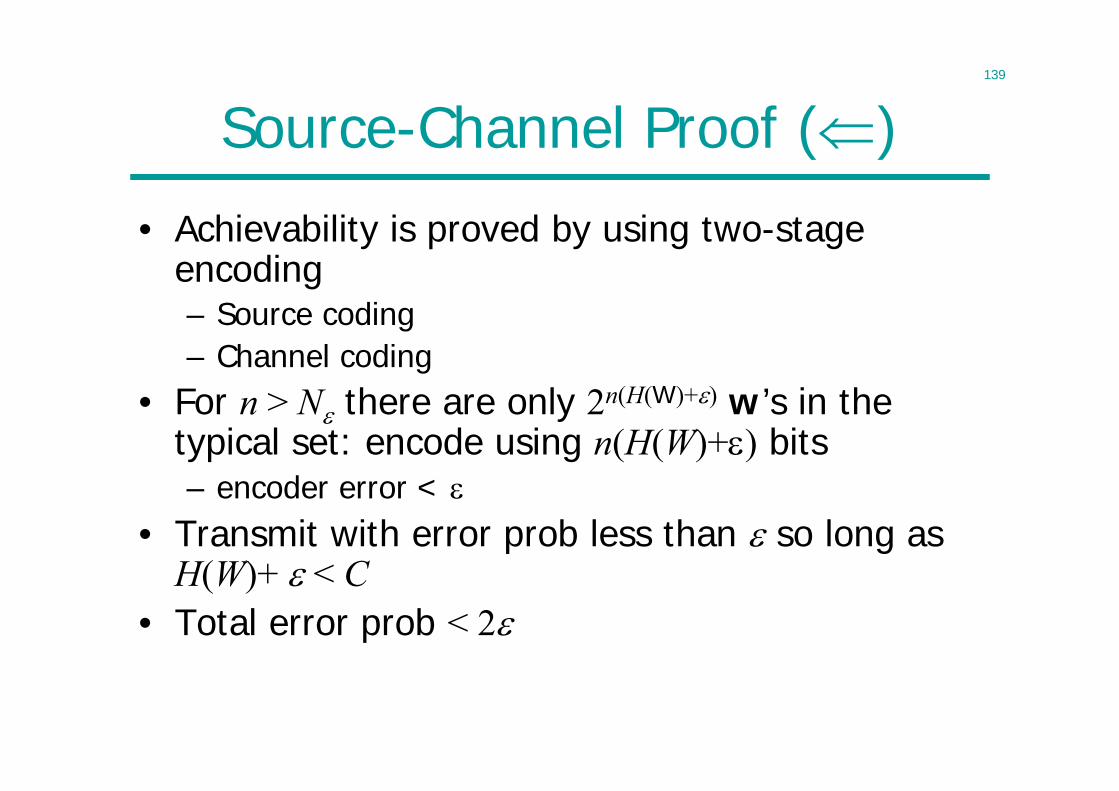
Source-Channel Proof ()
• Achievability is proved by using two-stage encoding– Source coding– Channel coding
• For n > N there are only 2n(H(W)+) w’s in the typical set: encode using n(H(W)+) bits– encoder error <
• Transmit with error prob less than so long as H(W)+ < C
• Total error prob < 2
140
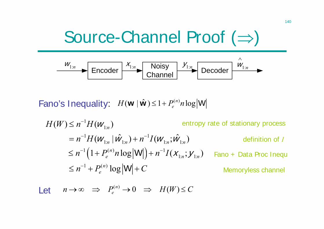
Source-Channel Proof ()
Fano’s Inequality: ( )ˆ( | ) 1 logneH P n w w W
11:( ) ( )nH W n H w entropy rate of stationary process
definition of I
Fano + Data Proc Inequ
Memoryless channel
Let ( ) 0 ( )nen P H W C
1 11: 1: 1: 1:
ˆ ˆ( | ) ( ; )n n n nn H n I w w w w
1 ( ) 11: 1:1 log ( ; )n
e n nn P n n I x yW1 ( ) logn
en P C W
NoisyChannel
x1:n y1:nEncoderw1:n Decoder
w1:n
141
Separation Theorem• Important result: source coding and channel coding
might as well be done separately since same capacity– Joint design is more difficult
• Practical implication: for a DMC we can design the source encoder and the channel coder separately– Source coding: efficient compression– Channel coding: powerful error-correction codes
• Not necessarily true for– Correlated channels– Multiuser channels
• Joint source-channel coding: still an area of research– Redundancy in human languages helps in a noisy environment
142
Summary
• Converse to channel coding theorem– Proved using Fano’s inequality– Capacity is a clear dividing point:
• If R < C, error prob. 0• Otherwise, error prob. 1
• Feedback doesn’t increase the capacity of DMC– May increase the capacity of memory channels (e.g.,
ARQ in TCP/IP)
• Source-channel separation theorem for DMC and stationary sources

143
Lecture 12
• Continuous Random Variables• Differential Entropy
– can be negative– not really a measure of the information in x– coordinate-dependent
• Maximum entropy distributions– Uniform over a finite range– Gaussian if a constant variance
144
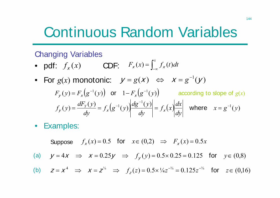
Continuous Random VariablesChanging Variables• pdf: CDF:)(xfx
x
dttfxF )()( xx
)()( 1 yxxy gg
)(1)()( 11 ygFygFyF xxy or
xxFxxf 5.0)()2,0(5.0)( xx for
)8,0(125.025.05.0)(25.04 yyf foryyxxy
)16,0(125.0¼5.0)( ¾¾¼4 zzzzf forzzxxz
(a)
(b)
Suppose
according to slope of g(x)
)()()()()( 11
1 ygxdydxxf
dyydgygf
dyydFyf Y
wherexxy
• Examples:
• For g(x) monotonic:
145
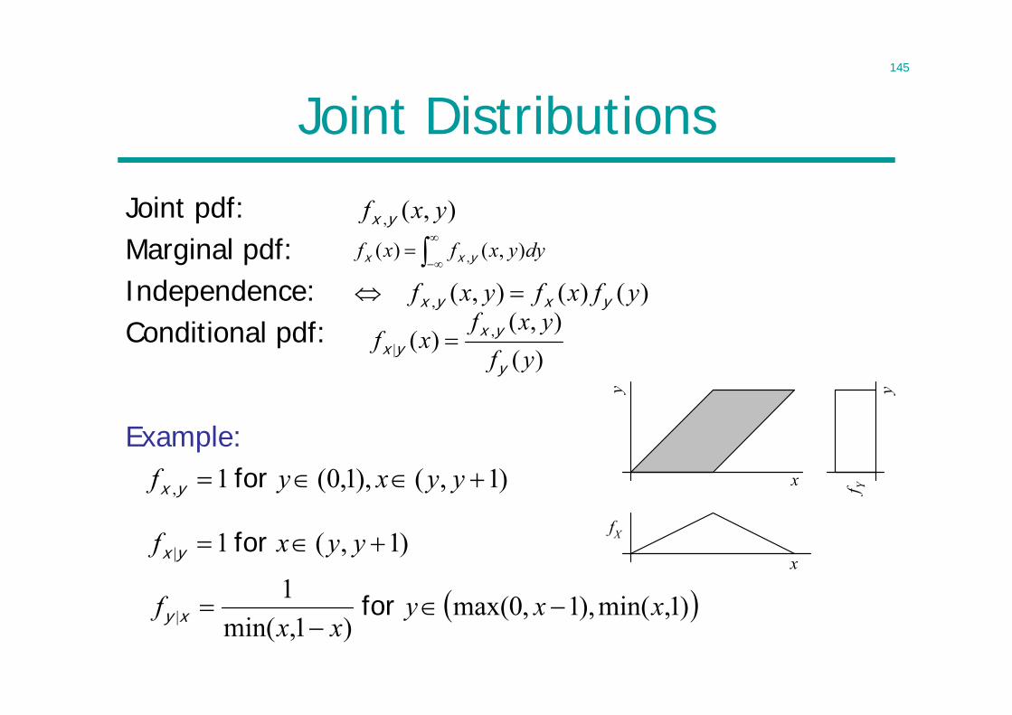
Joint Distributions
Joint pdf:Marginal pdf:Independence:Conditional pdf:
),(, yxf yx
dyyxfxf ),()( ,yxx
)(),(
)( ,| yf
yxfxf
y
yxyx
)()(),(, yfxfyxf yxyx
fX
x f Y
y
x
y
)1,(),1,0(1, yyxyf for yx
Example:
)1,(1| yyxf for yx
)1,min(),1,0max()1,min(
1| xxy
xxf
for xy
146
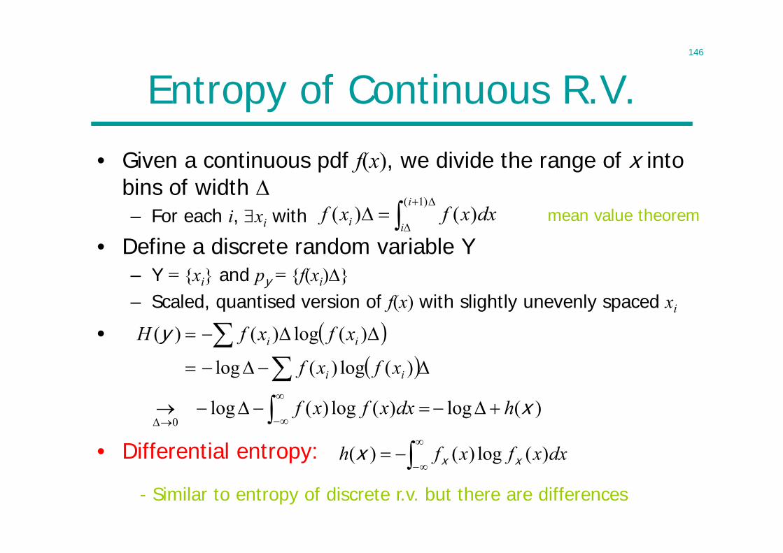
Entropy of Continuous R.V.
• Given a continuous pdf f(x), we divide the range of x into bins of width – For each i, xi with
• Define a discrete random variable Y– Y = {xi} and py = {f(xi)}– Scaled, quantised version of f(x) with slightly unevenly spaced xi
)1()()(
i
ii dxxfxf
)(log)(log)(log
)(log)(log
)(log)()(
0x
y
hdxxfxf
xfxf
xfxfH
ii
ii
dxxfxfh )(log)()( xxx
mean value theorem
• Differential entropy:
•
- Similar to entropy of discrete r.v. but there are differences
147
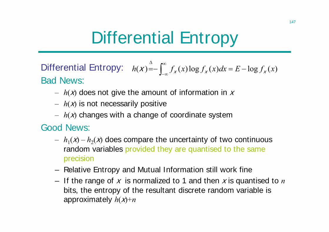
Differential Entropy
Differential Entropy: )(log)(log)()( xfEdxxfxfh xxxx
Good News:– h1(x) – h2(x) does compare the uncertainty of two continuous
random variables provided they are quantised to the same precision
– Relative Entropy and Mutual Information still work fine– If the range of x is normalized to 1 and then x is quantised to n
bits, the entropy of the resultant discrete random variable is approximately h(x)+n
Bad News:– h(x) does not give the amount of information in x– h(x) is not necessarily positive– h(x) changes with a change of coordinate system
148
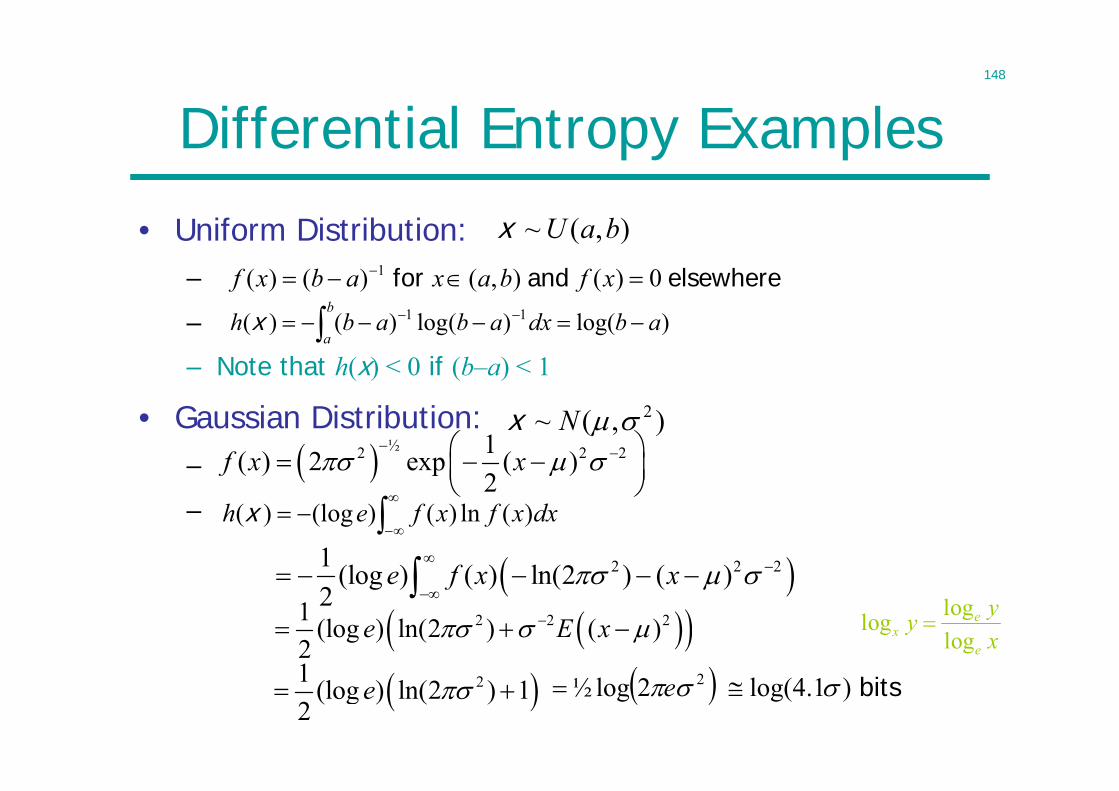
Differential Entropy Examples
• Uniform Distribution:–
–
– Note that h(x) < 0 if (b–a) < 1
),(~ baUx
elsewhere and for 0)(),()()( 1 xfbaxabxf
)log()(log)()( 11 abdxababhb
a x
),(~ 2Nx ½2 2 21( ) 2 exp ( )
2f x x
dxxfxfeh )(ln)()(log)(x
• Gaussian Distribution:–
–
2 2 21 (log ) ( ) ln(2 ) ( )2
e f x x
bits e )1.4log(2log½ 2
2 2 21 (log ) ln(2 ) ( )2
e E x
21 (log ) ln(2 ) 12
e
xyy
e
ex log
loglog
149
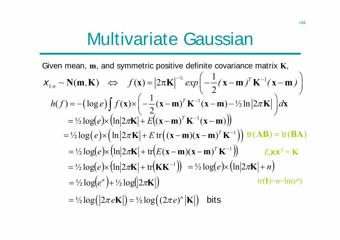
Multivariate GaussianGiven mean, m, and symmetric positive definite covariance matrix K,
11
1( ) ( ) 22
½ T:n ~ , f exp ( ) ( )
N m K x K x m K x mx
11( ) log ( ) ( ) ( ) ½ ln 22
Th f e f d x x m K x m K x
)()(2lnlog½ 1 mxKmxK TEe
1))((tr2lnlog½ KmxmxK TEe
1tr2lnlog½ KKKe ne K2lnlog½
K2log½log½ ne
½ log 2 ½ log (2 )ne e K K bits
1½ log ln 2 tr ( )( )Te E K x m x m K )(tr)(tr BAAB
EfxxT = K
tr(I)=n=ln(en)
150
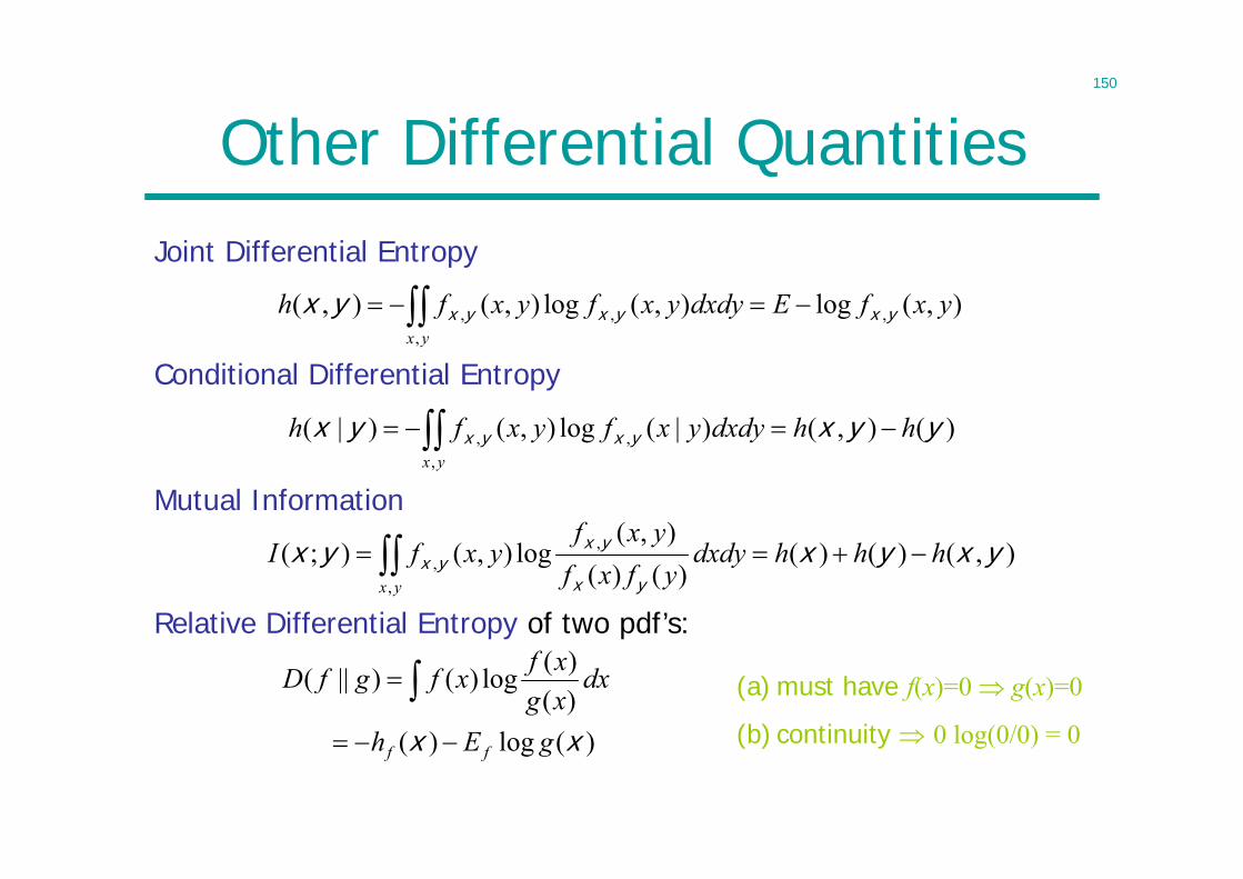
Other Differential QuantitiesJoint Differential Entropy
),(log),(log),(),( ,,
,, yxfEdxdyyxfyxfhyx
yxyxyxyx
)(),()|(log),()|(,
,, yyxyx yxyx hhdxdyyxfyxfhyx
)(log)()()(log)()||(
xx gEh
dxxgxfxfgfD
ff
),()()()()(
),(log),();(
,
,, yxyxyx
yx
yxyx hhhdxdy
yfxfyxf
yxfIyx
(a) must have f(x)=0 g(x)=0
(b) continuity 0 log(0/0) = 0
Relative Differential Entropy of two pdf’s:
Mutual Information
Conditional Differential Entropy
151
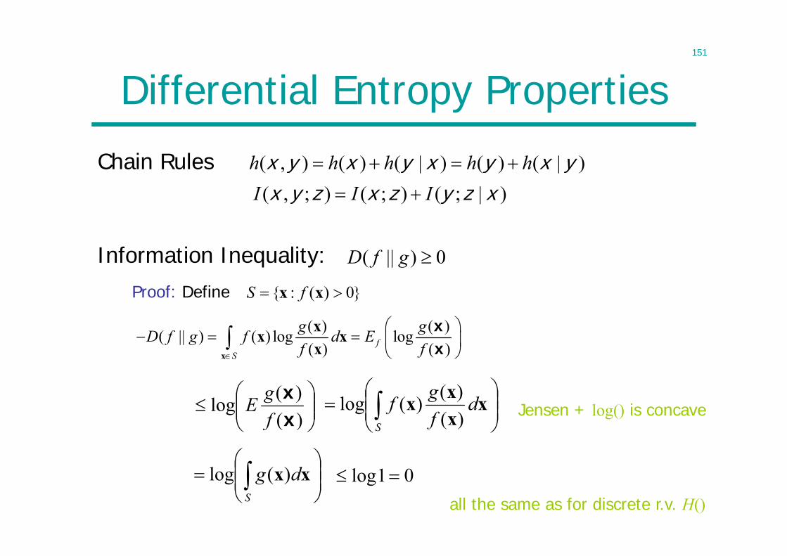
Differential Entropy Properties
Chain Rules )|()()|()(),( yxyxyxyx hhhhh
)|;();();,( xzyzxzyx III
0)||( gfD
( ) ( )( || ) ( ) log log( ) ( )f
S
g gD f g f d Ef f
x
xx xx
xx
Proof: Define }0)(:{ xx fS
Jensen + log() is concave
all the same as for discrete r.v. H()
Information Inequality:
)()(log
xx
fgE
S
dfgf x
xxx
)()()(log
S
dg xx)(log 01log
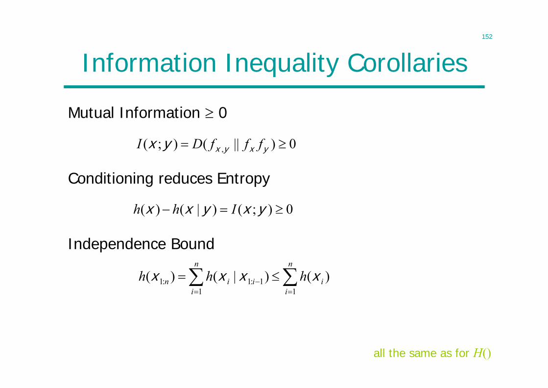
152
Information Inequality Corollaries
Mutual Information 0
0)||();( , yxyxyx fffDI
0);()|()( yxyxx Ihh
n
ii
n
iiin hhh
111:1:1 )()|()( xxxx
all the same as for H()
Independence Bound
Conditioning reduces Entropy
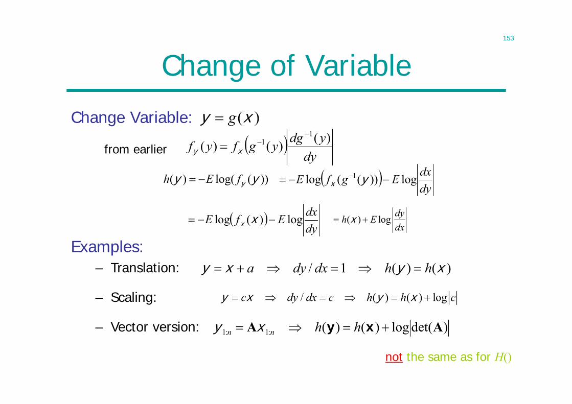
153
Change of Variable
Change Variable: )(xy g
dy
ydgygfyf )()()(1
1
xyfrom earlier
))(log()( yy yfEh
Examples:– Translation: )()(1/ xyxy hhdxdya
/ ( ) ( ) logc dy dx c h h c y x y x
not the same as for H()
)det(log)()(:1:1 AA xy hhnn xy
dydxEfE log)(log xx
dydxEgfE log))((log 1 yx
( ) log dyh Edx
x
– Vector version:
– Scaling:
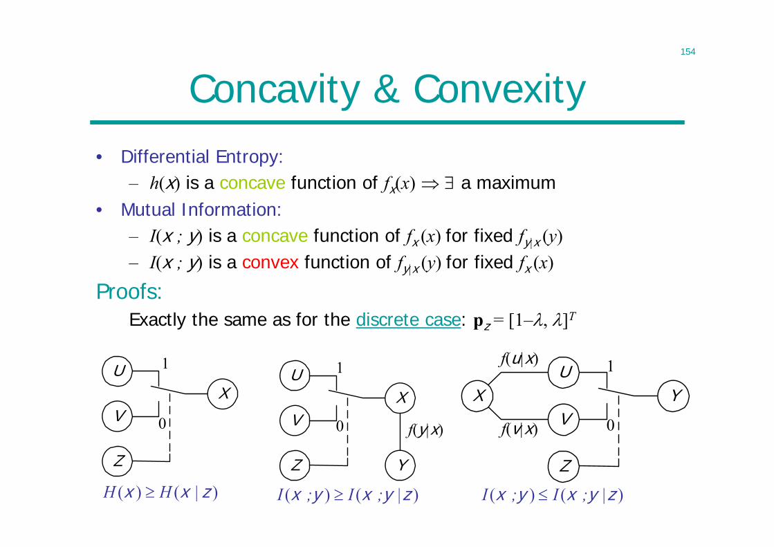
154
Concavity & Convexity• Differential Entropy:
– h(x) is a concave function of fx(x) a maximum• Mutual Information:
– I(x ; y) is a concave function of fx (x) for fixed fy|x (y)– I(x ; y) is a convex function of fy|x (y) for fixed fx (x)
U
VX
Z
1
0
U
VX
Z Y
f(y|x)
1
0
U
VY
Z
f(u|x)
X
f(v|x)
1
0
)|()( zxx HH )()( zyxyx |;I;I )()( zyxyx |;I;I
Proofs:Exactly the same as for the discrete case: pz = [1–, ]T
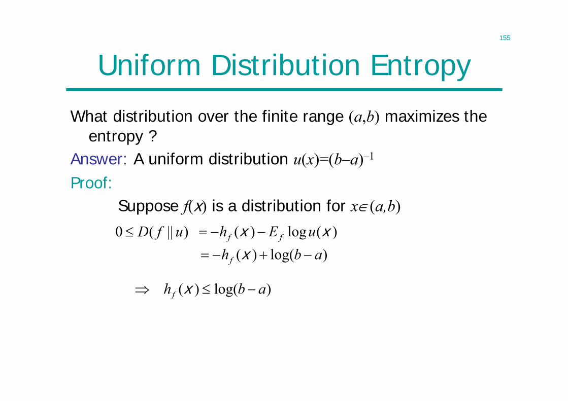
155
Uniform Distribution Entropy
What distribution over the finite range (a,b) maximizes the entropy ?
Answer: A uniform distribution u(x)=(b–a)–1
)||(0 ufD
Proof:Suppose f(x) is a distribution for x(a,b)
)(log)( xx uEh ff
)log()( abhf x
)log()( abhf x
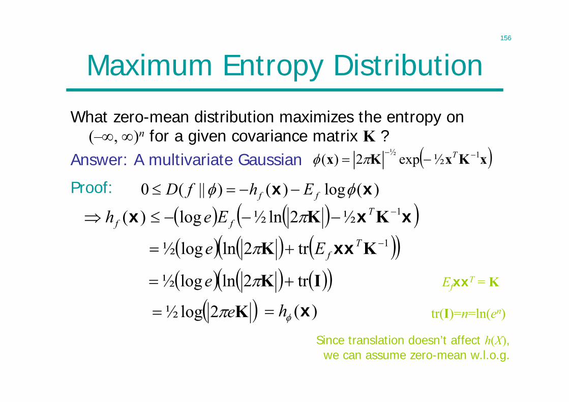
156
Maximum Entropy Distribution
What zero-mean distribution maximizes the entropy on(–, )n for a given covariance matrix K ?
Answer: A multivariate Gaussian xKxKx 1½ ½exp2)( T
)(log)()||(0 xx ff EhfD
Since translation doesn’t affect h(X), we can assume zero-mean w.l.o.g.
EfxxT = K
tr(I)=n=ln(en)
Proof:
Ke2log½
xxx 1½2ln½log)( KK Tff Eeh
1tr2lnlog½ KK TfEe xx
IK tr2lnlog½ e
)(xh
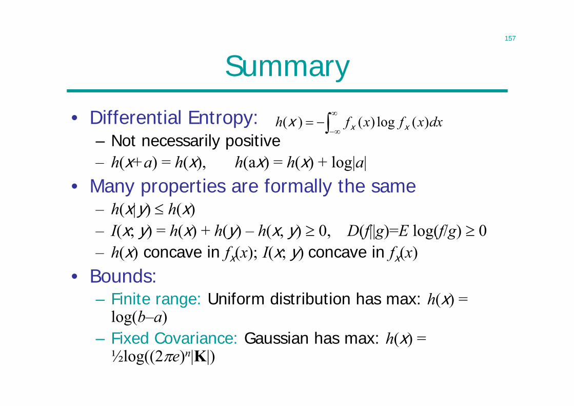
157
Summary
• Differential Entropy:– Not necessarily positive– h(x+a) = h(x), h(ax) = h(x) + log|a|
• Many properties are formally the same– h(x|y) h(x) – I(x; y) = h(x) + h(y) – h(x, y) 0, D(f||g)=E log(f/g) 0– h(x) concave in fx(x); I(x; y) concave in fx(x)
• Bounds:– Finite range: Uniform distribution has max: h(x) =
log(b–a)– Fixed Covariance: Gaussian has max: h(x) =
½log((2e)n|K|)
dxxfxfh )(log)()( xxx
158
Lecture 13
• Discrete-Time Gaussian Channel Capacity• Continuous Typical Set and AEP• Gaussian Channel Coding Theorem• Bandlimited Gaussian Channel
– Shannon Capacity
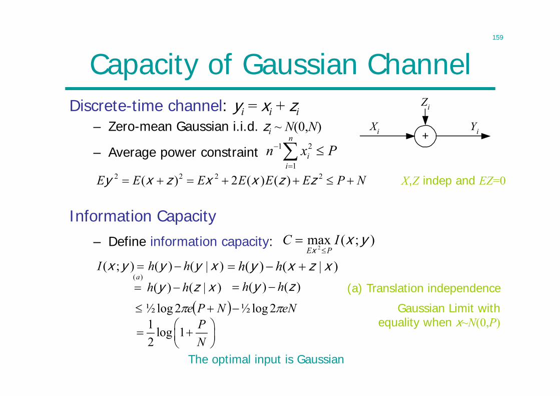
159
Capacity of Gaussian ChannelDiscrete-time channel: yi = xi + zi
– Zero-mean Gaussian i.i.d. zi ~ N(0,N)
– Average power constraint+
Xi Yi
Zi
Pxnn
ii
1
21
);(max2
yxx
ICPE
)|()( xzxy hh(a) Translation independence
NPEEEEEE 2222 )()(2)( zzxxzxy X,Z indep and EZ=0
Gaussian Limit withequality when x~N(0,P)
The optimal input is Gaussian
Information Capacity– Define information capacity:
)|()();( xyyyx hhI
)|()()(
xzy hha
1 log 12
PN
)()( zy hh
eNNPe 2log½2log½
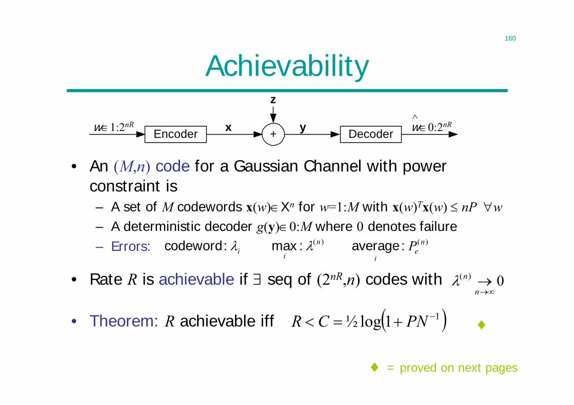
160
Achievability
• An (M,n) code for a Gaussian Channel with power constraint is– A set of M codewords x(w)Xn for w=1:M with x(w)Tx(w) nP w– A deterministic decoder g(y)0:M where 0 denotes failure– Errors: )()( n
ei
n
ii P:average :max :codeword
0)(
n
n
11log½ PNCR
+
z
Encoder Decoderx yw1:2nR w0:2nR^
= proved on next pages
• Theorem: R achievable iff
• Rate R is achievable if seq of (2nR,n) codes with
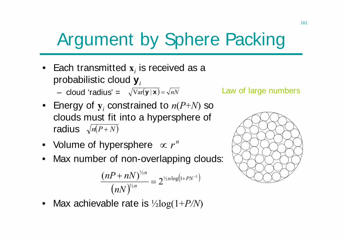
161
• Volume of hypersphere• Max number of non-overlapping clouds:
Argument by Sphere Packing• Each transmitted xi is received as a
probabilistic cloud yi– cloud ‘radius’ = nNxy |Var
NPn
nr
11log½
½
½
2)( PNn
n
n
nNnNnP
• Max achievable rate is ½log(1+P/N)
• Energy of yi constrained to n(P+N) so clouds must fit into a hypersphere of radius
Law of large numbers
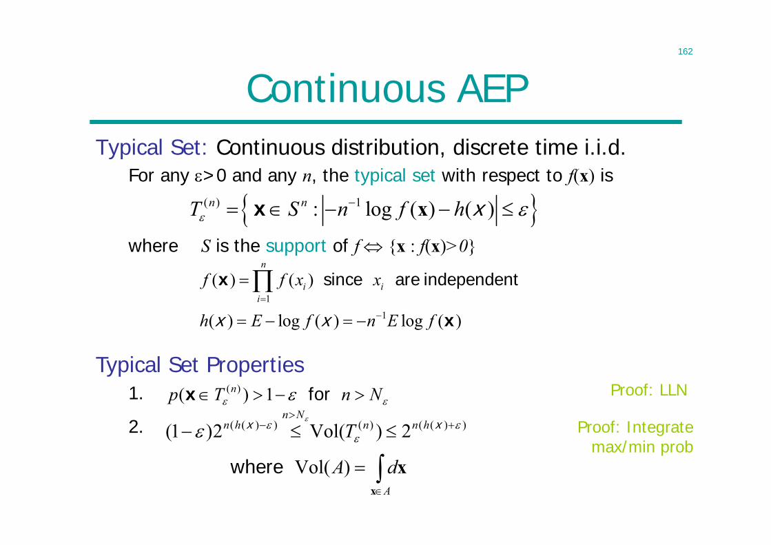
162
Continuous AEPTypical Set: Continuous distribution, discrete time i.i.d.
For any >0 and any n, the typical set with respect to f(x) is
( ) 1: log ( ) ( )n nT S n f h x xx
1
1
( ) ( )
( ) log ( ) log ( )
n
i ii
f f x x
h E f n E f
x x
x
x
since are independent
NnTp n for 1)( )(x))(()())(( 2)Vol(2)1(
xx hnnNn
hn T
Proof: LLN
Proof: Integrate max/min prob
A
dAx
x)Vol( where
Typical Set Properties1.
where S is the support of f {x : f(x)>0}
2.
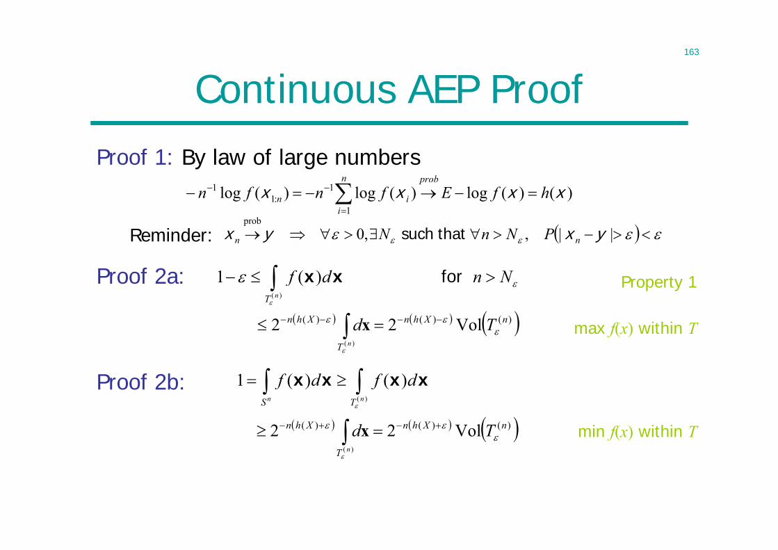
163
Continuous AEP ProofProof 1: By law of large numbers
)()(log)(log)(log1
1:1
1 xxxx hfEfnfnprobn
iin
||,,0prob
yxyx nn PNnN that such
)()()( Vol22)(
nXhn
T
Xhn Tdn
x
( )
1 ( ) ( )n nS T
f d f d
x x x x
max f(x) within T
Property 1
min f(x) within T
Proof 2b:
Proof 2a:
Reminder:
( )
1 ( )nT
f d n N
x x for
)()()( Vol22)(
nXhn
T
Xhn Tdn
x

164
Jointly Typical SetJointly Typical: xi, yi i.i.d from 2 with fx,y (xi,yi)
( ) 2 1
1
1,
, : log ( ) ( ) ,
log ( ) ( ) ,
log ( , ) ( , )
n nX
Y
X Y
J n f h
n f h
n f h
x
y
x y
x y x
y
x y
( ),, log , ( , )nJ f nh n x y x yx y x y
NnJp n for1, )(yx
),()(),( 2Vol2)1( yxyx hnnNn
hn J
3);()(3);( 2','2)1(
yxyx InnNn
In Jp yx
Proof of 4.: Integrate max/min f(x´, y´)=f(x´)f(y´), then use known bounds on Vol(J)
4. Indep x′,y′:
3. Size:
2. Total Prob:
Properties:
1. Indiv p.d.:
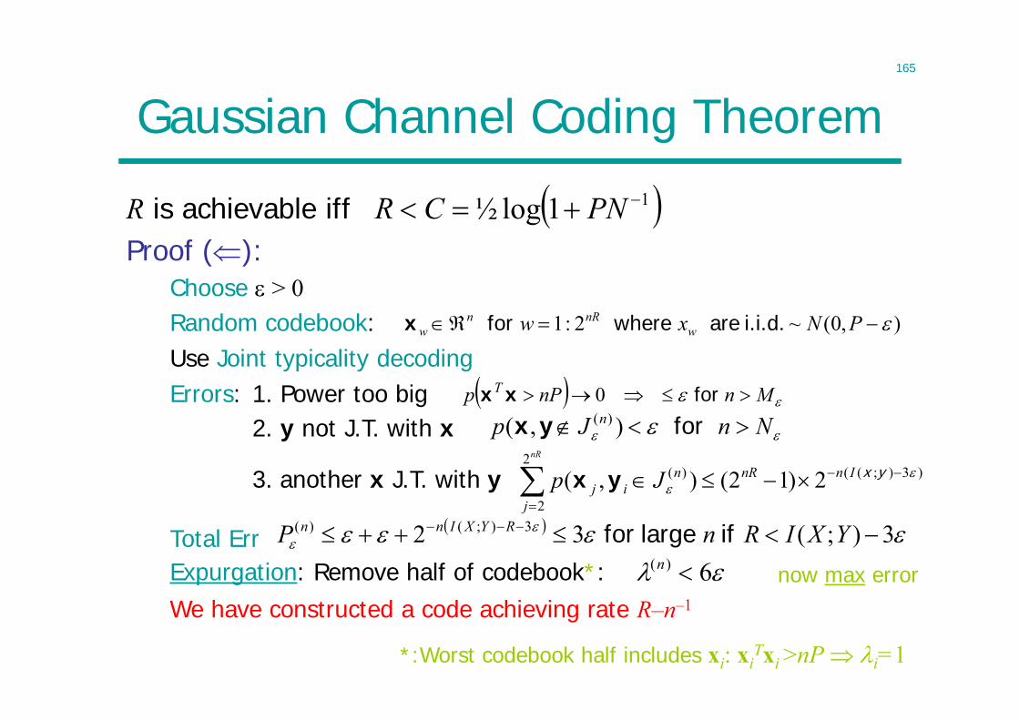
165
Gaussian Channel Coding Theorem
R is achievable iff 11log½ PNCR
),0(~2:1 PNxw wnRn
w i.i.d. are where for x
MnnPp T for 0xx
NnJp n for ),( )(yx
)3);((2
2
)( 2)12(),(
yxInnR
j
nij
nR
Jp yx
3);(32 3);()( YXIRnP RYXInn if largefor
6)( n
*:Worst codebook half includes xi: xiTxi >nP i=1
now max error
We have constructed a code achieving rate R–n–1
Expurgation: Remove half of codebook*: Total Err
3. another x J.T. with y
2. y not J.T. with xErrors: 1. Power too bigUse Joint typicality decodingRandom codebook:
Proof ():Choose > 0
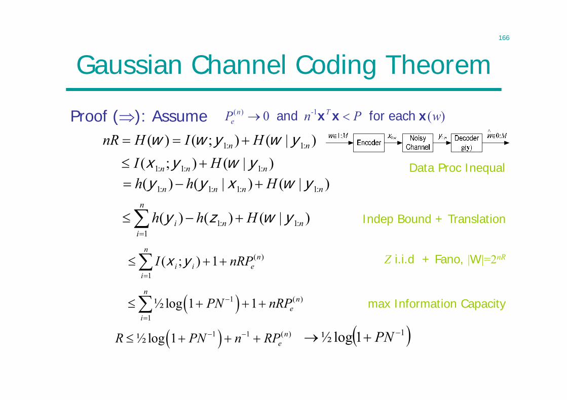
166
Gaussian Channel Coding Theorem
Proof (): Assume ( ) 10 ( )n - TeP n P w x x x and for each
11log½ PN
Data Proc Inequal
Indep Bound + Translation
Z i.i.d + Fano, |W|=2nR
max Information Capacity
)|();()( :1:1 nn HIHnR ywyww
)|();( :1:1:1 nnn HI ywyx )|()|()( :1:1:1:1 nnnn Hhh ywxyy
)|()()( :1:11
nn
n
ii Hhh ywzy
( )
1( ; ) 1
nn
i i ei
I nRP
x y
1 ( )
1½ log 1 1
nn
ei
PN nRP
1 1 ( )½ log 1 neR PN n RP
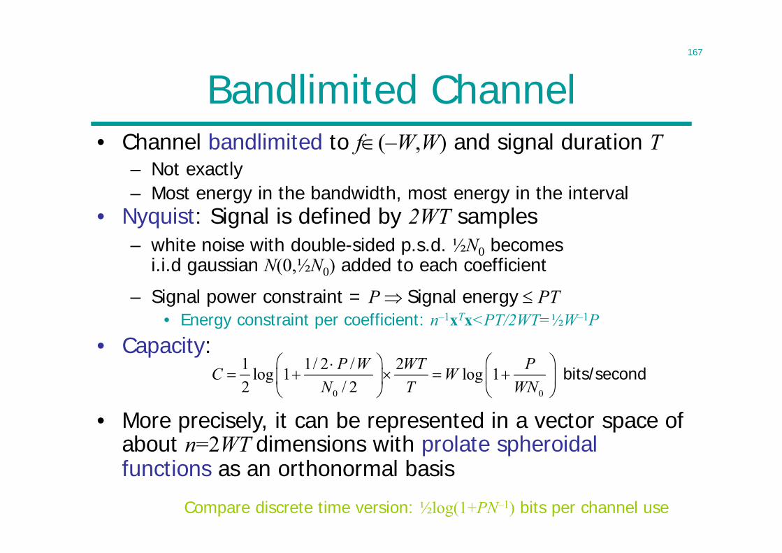
167
Bandlimited Channel• Channel bandlimited to f(–W,W) and signal duration T
– Not exactly– Most energy in the bandwidth, most energy in the interval
0 0
1 1/ 2 / 2log 1 log 12 / 2
P W WT PC WN T WN
bits/second
Compare discrete time version: ½log(1+PN–1) bits per channel use
• Capacity:
– Signal power constraint = P Signal energy PT• Energy constraint per coefficient: n–1xTx<PT/2WT=½W–1P
– white noise with double-sided p.s.d. ½N0 becomesi.i.d gaussian N(0,½N0) added to each coefficient
• More precisely, it can be represented in a vector space of about n=2WT dimensions with prolate spheroidal functions as an orthonormal basis
• Nyquist: Signal is defined by 2WT samples
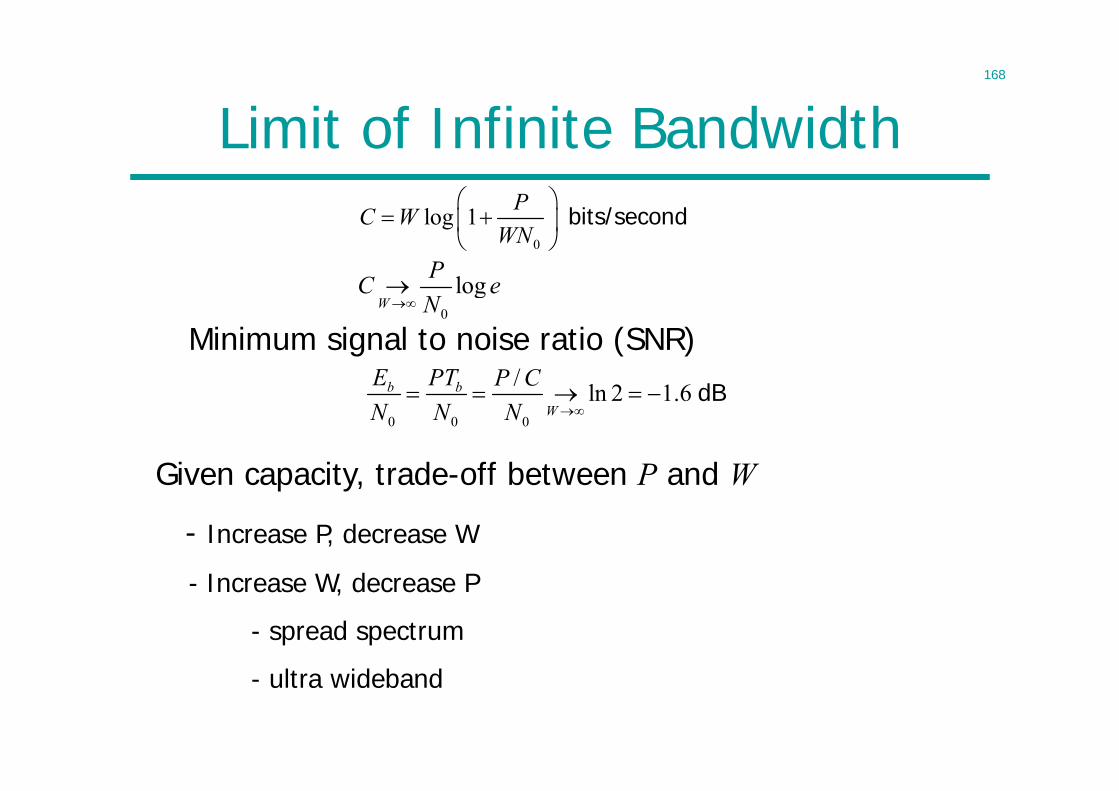
168
Limit of Infinite Bandwidth
Minimum signal to noise ratio (SNR) 0
logW
PC eN
0 0 0
/ ln 2 1.6b b
W
E PT P CN N N
dB
0
log 1 PC WWN
bits/second
Given capacity, trade-off between P and W
- Increase P, decrease W
- Increase W, decrease P
- spread spectrum
- ultra wideband
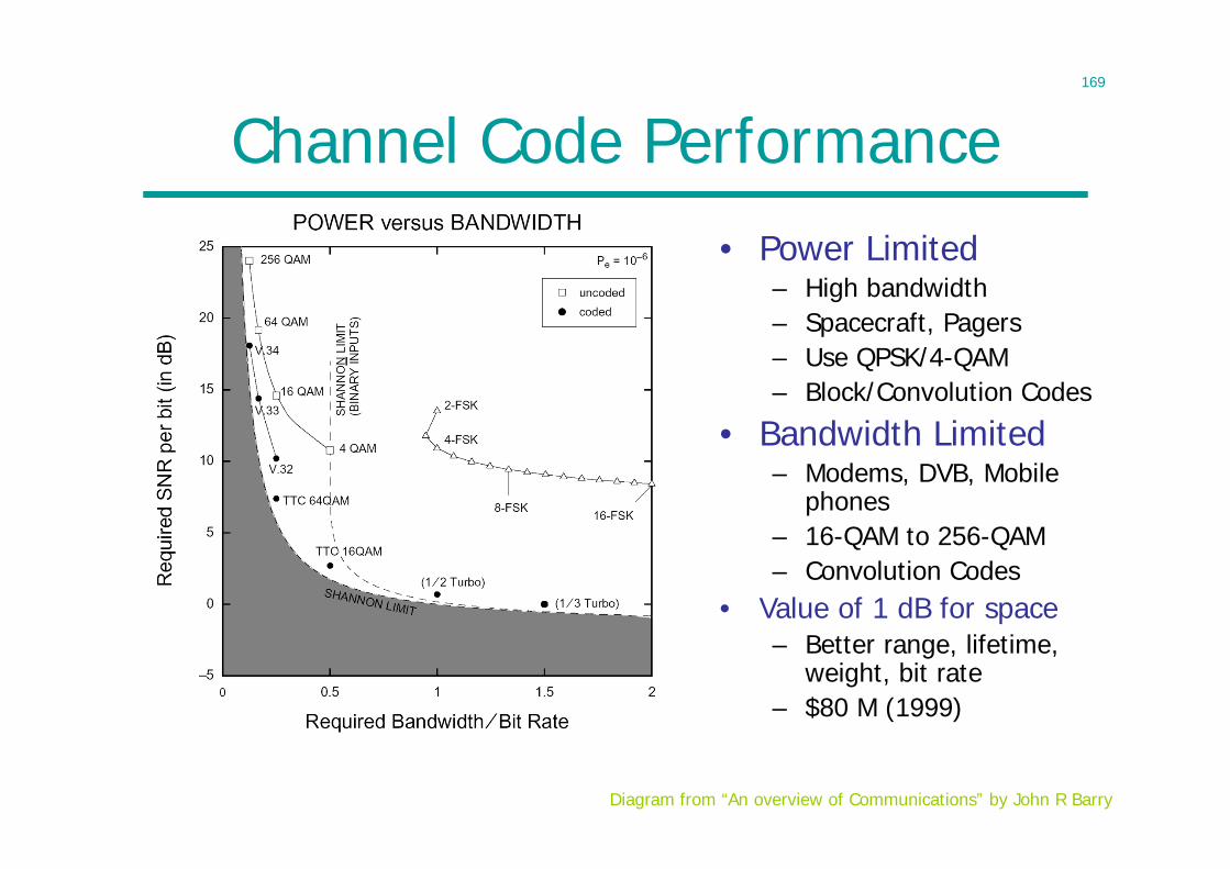
169
Channel Code Performance• Power Limited
– High bandwidth– Spacecraft, Pagers– Use QPSK/4-QAM– Block/Convolution Codes
Diagram from “An overview of Communications” by John R Barry
• Value of 1 dB for space– Better range, lifetime,
weight, bit rate– $80 M (1999)
• Bandwidth Limited– Modems, DVB, Mobile
phones– 16-QAM to 256-QAM– Convolution Codes
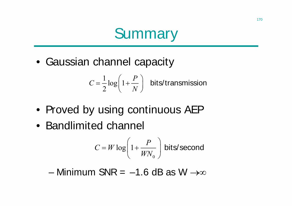
170
Summary
• Gaussian channel capacity
• Proved by using continuous AEP• Bandlimited channel
– Minimum SNR = –1.6 dB as W
1 log 12
PCN
bits/transmission
0
log 1 PC WWN
bits/second
171
Lecture 14
• Parallel Gaussian Channels– Waterfilling
• Gaussian Channel with Feedback– Memoryless: no gain– Memory: at most ½ bits/transmission
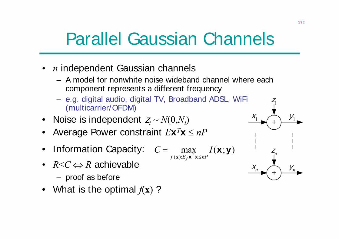
172
Parallel Gaussian Channels• n independent Gaussian channels
– A model for nonwhite noise wideband channel where each component represents a different frequency
– e.g. digital audio, digital TV, Broadband ADSL, WiFi (multicarrier/OFDM)
• Noise is independent zi ~ N(0,Ni)• Average Power constraint ExTx nP
+x1 y1
z1
+xn yn
zn( ):max ( ; )
Tff E nP
C I
x x x
x y
• What is the optimal f(x) ?
• R<C R achievable– proof as before
• Information Capacity:
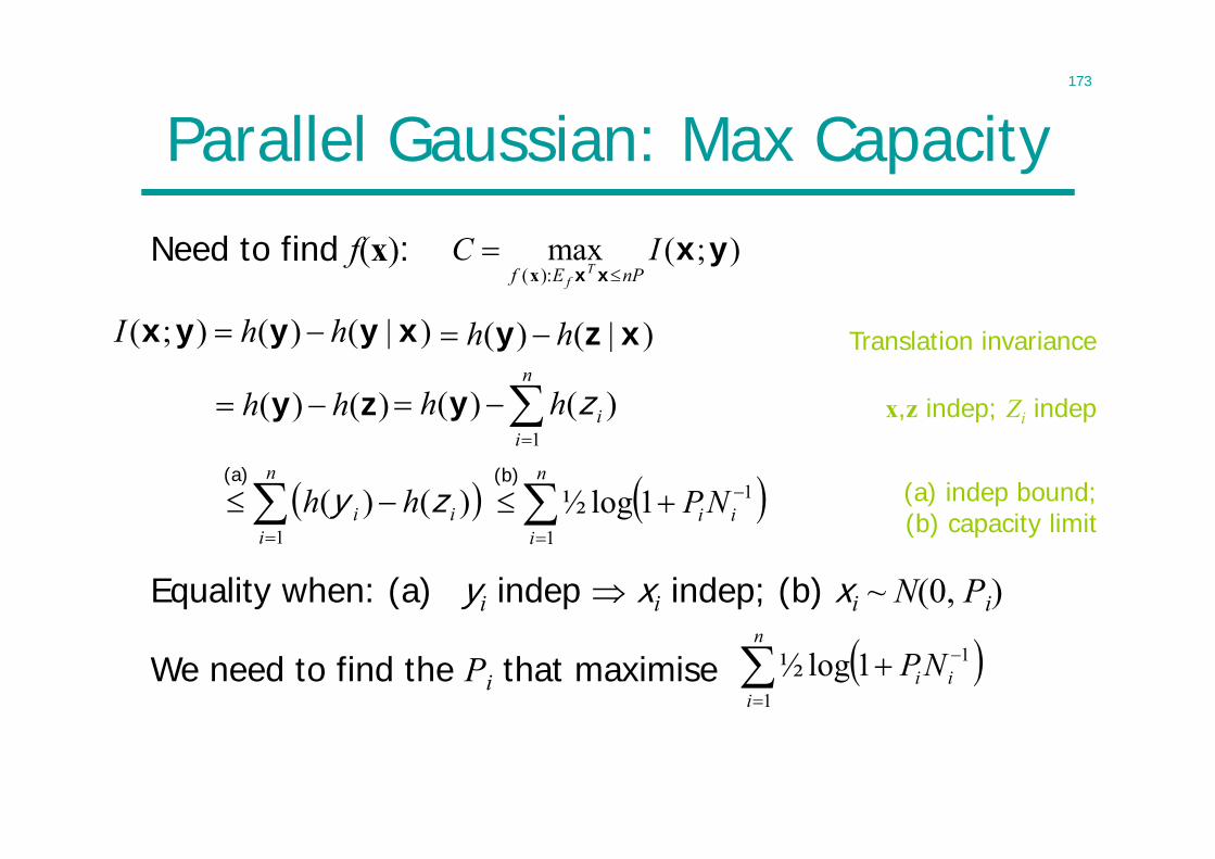
173
Parallel Gaussian: Max Capacity
Need to find f(x):
n
iii NP
1
11log½(b)
Translation invariance
x,z indep; Zi indep
(a) indep bound;(b) capacity limit
Equality when: (a) yi indep xi indep; (b) xi ~ N(0, Pi)
n
iii NP
1
11log½
( ):max ( ; )
Tff E nP
C I
x x x
x y
We need to find the Pi that maximise
)|()();( xyyyx hhI )|()( xzy hh
)()( zy hh
n
iihh
1
)()( zy
n
iii hh
1
)()( zy(a)
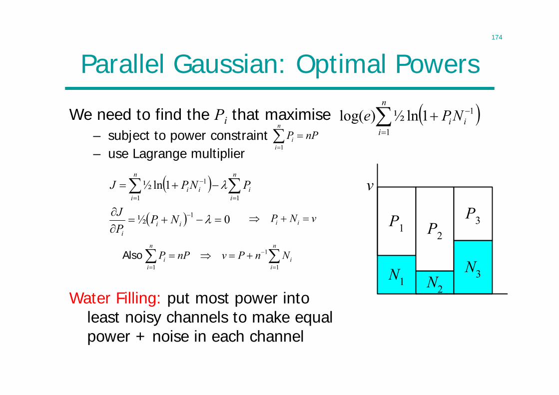
174
Parallel Gaussian: Optimal Powers
We need to find the Pi that maximise– subject to power constraint
n
iii NPe
1
11ln½)log(
i iP N v
1
n
ii
P nP
1
1 1
n n
i ii i
P nP v P n N
Also
Water Filling: put most power into least noisy channels to make equal power + noise in each channel
N1
P1
N2
P2
N3
P3
v
– use Lagrange multiplier
n
ii
n
iii PNPJ
11
11ln½
0½ 1 ii
i
NPPJ
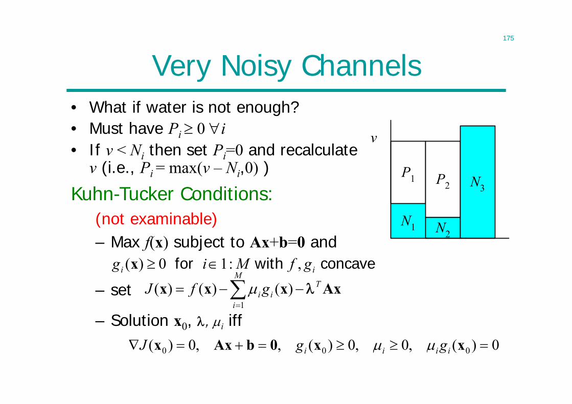
175
Very Noisy Channels• What if water is not enough?• Must have Pi 0 i• If v < Ni then set Pi=0 and recalculate
v (i.e., Pi = max(v – Ni,0) )
N1
P1
N2
P2 N3
v
Kuhn-Tucker Conditions:(not examinable)– Max f(x) subject to Ax+b=0 and
concave with for ii gfMig ,:10)( xAxxxx T
M
iii gfJ
1
)()()(
0)(,0,0)(,,0)( 000 xx0bAxx iiii ggJ – Solution x0, , i iff
– set
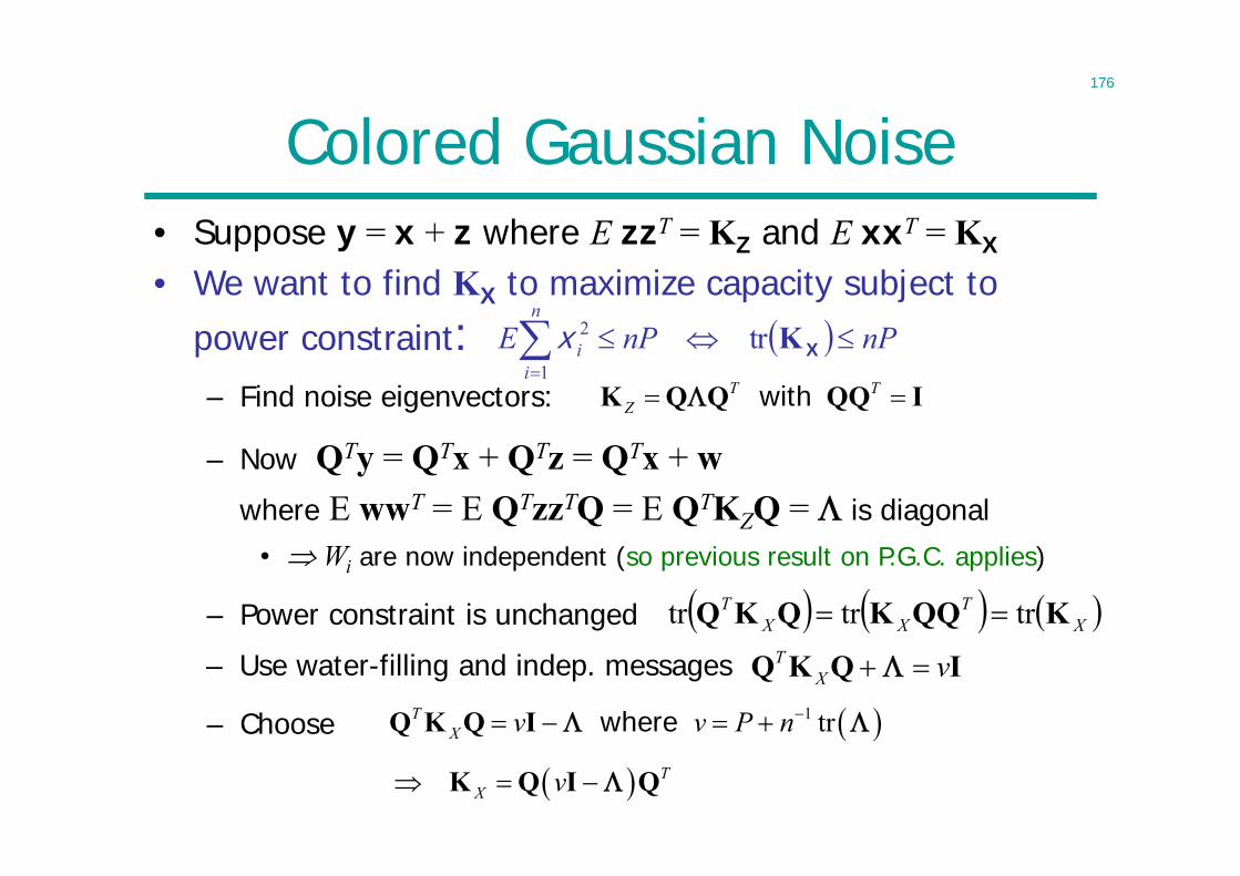
176
Colored Gaussian Noise• Suppose y = x + z where E zzT = KZ and E xxT = KX
nPnPEn
ii
XKtr
1
2xT T
Z K Q Q QQ I with
XT
XXT KQQKQKQ trtrtr
1 trTX v v P n Q K Q I where
TX v K Q I Q
– Choose
– Power constraint is unchanged
• Wi are now independent (so previous result on P.G.C. applies)
– Now QTy = QTx + QTz = QTx + wwhere E wwT = E QTzzTQ = E QTKZQ = is diagonal
– Find noise eigenvectors:
• We want to find KX to maximize capacity subject to power constraint:
– Use water-filling and indep. messages TX v Q K Q I
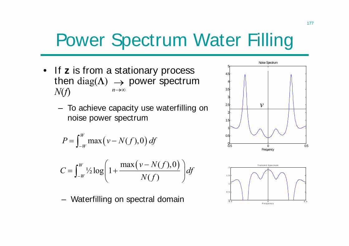
177
Power Spectrum Water Filling• If z is from a stationary process
then diag() power spectrum N(f)
-0.5 0 0.50
0.5
1
1.5
2
2.5
3
3.5
4
4.5
5
Frequency
Noise Spectrum
-0 .5 0 0 .50
0 .5
1
1 .5
2
F re q u e n c y
T ra n s m it S p e c tru m max ( ),0½log 1
( )W
W
v N fC df
N f
max ( ),0W
WP v N f df
n
– To achieve capacity use waterfilling on noise power spectrum
v
– Waterfilling on spectral domain
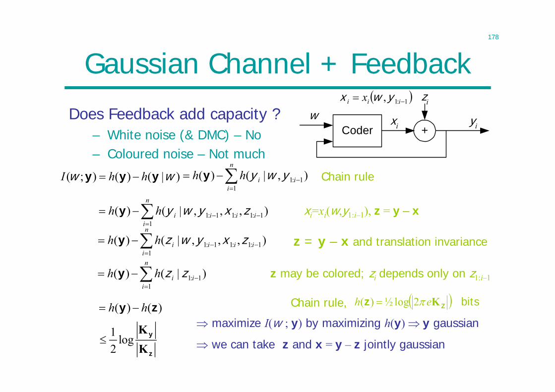
178
Gaussian Channel + Feedback
Does Feedback add capacity ?+
xi yi
zi
Coderw
1:1, iii x ywx
1 log2
KK
y
z
xi=xi(w,y1:i–1), z = y – x
z = y – x and translation invariance
z may be colored; zi depends only on z1:i–1
maximize I(w ; y) by maximizing h(y) y gaussian
we can take z and x = y – z jointly gaussian
Chain rule
Chain rule, bitsZz Keh 2log½)(
– White noise (& DMC) – No– Coloured noise – Not much
)|()();( ww yyy hhI
n
iiihh
11:1 ),|()( ywyy
n
iiiiihh
11:1:11:1 ),,,|()( zxywyy
n
iiiiihh
11:1:11:1 ),,,|()( zxywzy
n
iiihh
11:1 )|()( zzy
)()( zy hh
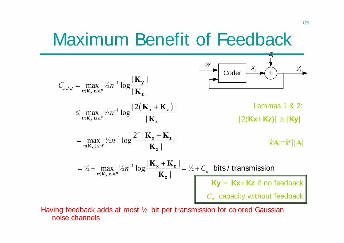
179
Maximum Benefit of Feedback
Having feedback adds at most ½ bit per transmission for colored Gaussian noise channels
1
tr( )
| |½ max ½ log ½
| | nnPn C
K
K KKx
x z
z
bits / transmission
|kA|=kn|(A|
Lemmas 1 & 2:
|2(Kx+Kz)| |Ky|
+xi yi
zi
Coderw
1, tr( )
| |max ½ log
| |n FB nPC n
K
KKx
y
z
1
tr( )
| 2 |max ½ log
| |nPn
K
K KKx
x z
z
1
tr( )
2 | |max ½ log
| |
n
nPn
K
K KKx
x z
z
Ky = Kx+Kz if no feedback
Cn: capacity without feedback
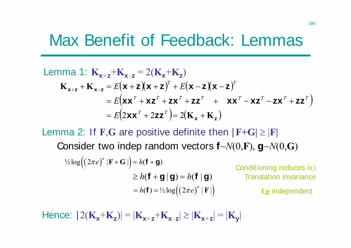
180
Max Benefit of Feedback: Lemmas
Lemma 1: Kx+z+Kx–z = 2(Kx+Kz) zx
zxzx
zzxx
zzzxxzxxzzzxxzxx
zxzxzxzx
KK
KK
222 TT
TTTTTTTT
TT
E
E
EE
Lemma 2: If F,G are positive definite then |F+G| |F|
Conditioning reduces h()Translation invariance
f,g independent
Hence: |2(Kx+Kz)| = |Kx+z+Kx–z| |Kx+z| = |Ky|
½ log 2 | | ( )ne h F G f g
)|()|( gfggf hh
( ) ½ log 2 | |nh e Ff
Consider two indep random vectors f~N(0,F), g~N(0,G)
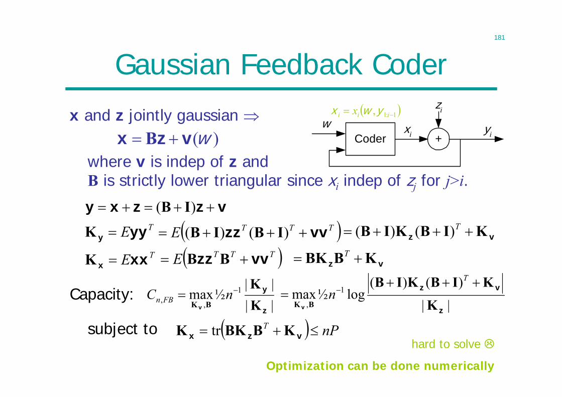
181
Gaussian Feedback Coder
x and z jointly gaussian
where v is indep of z andB is strictly lower triangular since xi indep of zj for j>i.
+xi yi
zi
Coderw
1:1, iii x ywx
)(wvzx B
Capacity:
subject to||
)()(log½max 1
,z
vz
v KKIBKIB
BK
T
n
nPT vzx KBBKK trhard to solve
Optimization can be done numerically
vzzxy )( IBTEyyy K TTTE vvzz )()( IBIB vz KIBKIB T)()(TExxx K TTTE vvzz BB vz KBBK T
||||
½max 1
,,z
y
v KK
BK
nC FBn
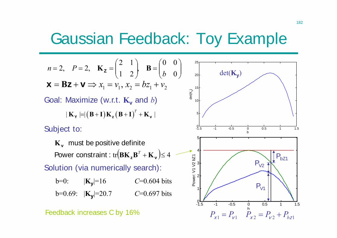
182
-1.5 -1 -0.5 0 0.5 1 1.50
1
2
3
4
5
b
Pow
er: V
1 V2
bZ1
Gaussian Feedback: Toy Example
000
,2112
,2,2b
Pn BKZ
-1.5 -1 -0.5 0 0.5 1 1.50
5
10
15
20
25
b
det(K
Y)
det(Ky)
PbZ1
PV1
PV2
1 1 2 1 2,x v x bz v x z vB
| | | |T K B I K B I KY z v
Goal: Maximize (w.r.t. Kv and b)
Subject to:
4tr vz
v
KBBK
KT :constraintPower
definite positive bemust
Solution (via numerically search):
b=0: |Ky|=16 C=0.604 bits
Feedback increases C by 16% 12211 zvxvx bPPPPP
b=0.69: |Ky|=20.7 C=0.697 bits
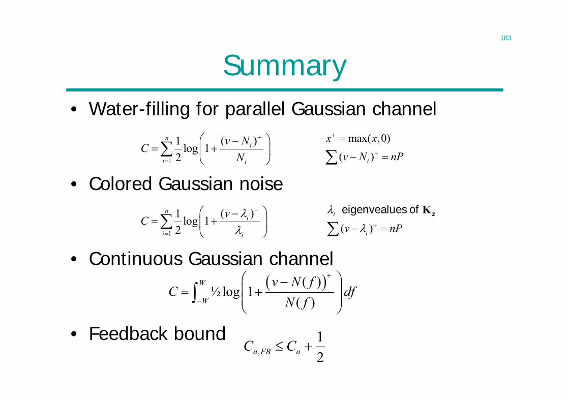
183
Summary• Water-filling for parallel Gaussian channel
• Colored Gaussian noise
• Continuous Gaussian channel
• Feedback bound
1
( )1 log 12
ni
i i
v NCN
max( ,0)( )i
x xv N nP
( )½log 1
( )W
W
v N fC df
N f
,12n FB nC C
1
( )1 log 12
ni
i i
vC
( )
i
iv nP
Κeigenvealues of z
184
Lecture 15
• Lossy Source Coding– For both discrete and continuous sources – Bernoulli Source, Gaussian Source
• Rate Distortion Theory– What is the minimum distortion achievable at
a particular rate?– What is the minimum rate to achieve a
particular distortion?
• Channel/Source Coding Duality
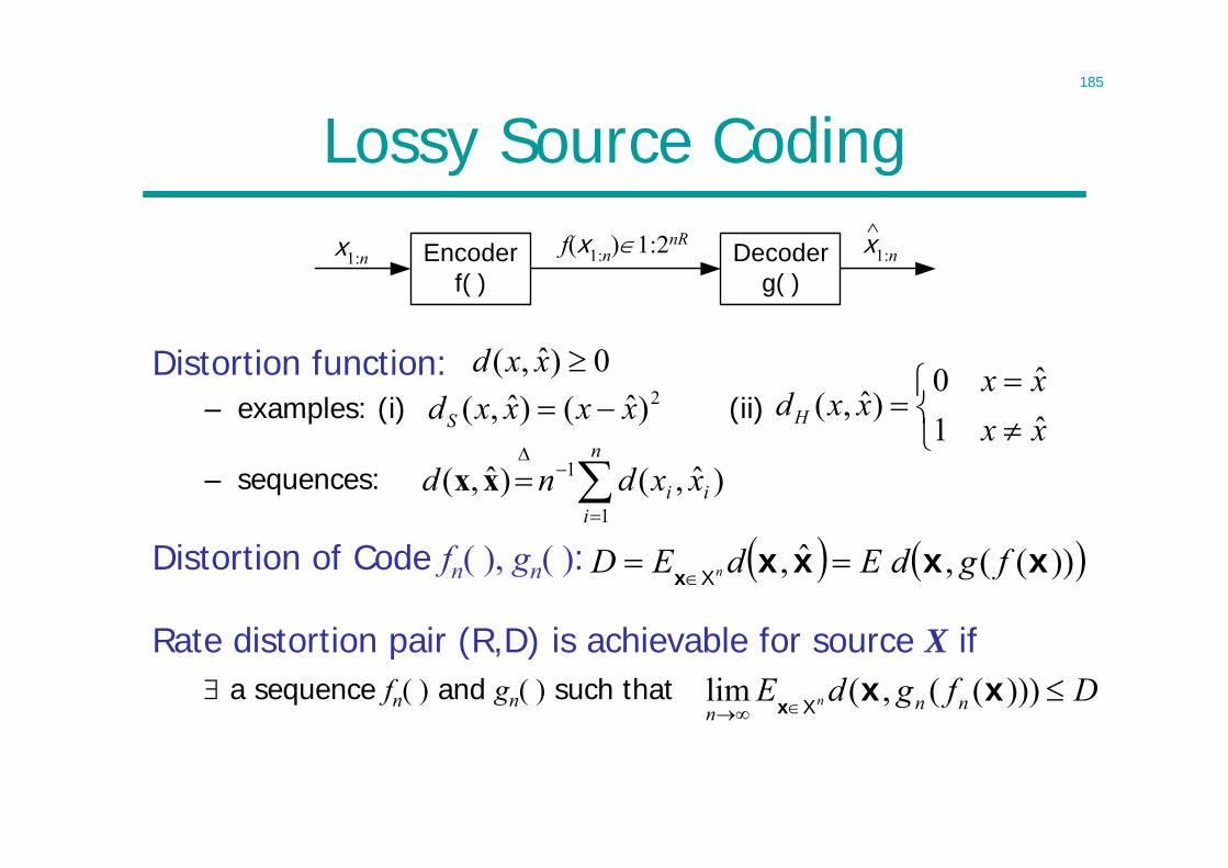
185
Lossy Source Coding
Distortion function:– examples: (i) (ii)
x1:n Encoderf( )
f(x1:n)1:2nRDecoder
g( )x1:n^
0)ˆ,( xxd2)ˆ()ˆ,( xxxxdS
xxxx
xxdH ˆ1ˆ0
)ˆ,(
n
iii xxdnd
1
1 )ˆ,()ˆ,( xx
))((,ˆ, xxxxx fgdEdED n X
DfgdE nnnn
)))((,(lim xx
x X
Rate distortion pair (R,D) is achievable for source X if a sequence fn( ) and gn( ) such that
Distortion of Code fn( ), gn( ):
– sequences:
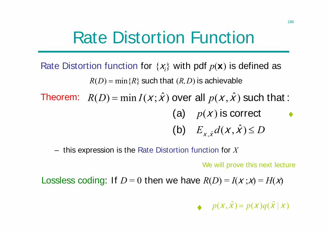
186
Rate Distortion FunctionRate Distortion function for {xi} with pdf p(x) is defined as
DdEp
pIDR
)ˆ,()(
)ˆ,()ˆ;(min)(
ˆ, xxx
xxxx
xx(b)
correct is (a):that such allover
( ) min{ } ( )R D R R,D such that is achievable
We will prove this next lecture
Lossless coding: If D = 0 then we have R(D) = I(x ;x) = H(x)
– this expression is the Rate Distortion function for X
Theorem:
ˆ ˆ( , ) ( ) ( | )p p qx x x x x
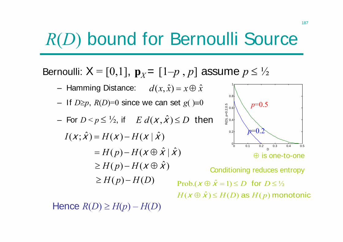
187
R(D) bound for Bernoulli Source
Bernoulli: X = [0,1], pX = [1–p , p] assume p ½– Hamming Distance: xxxxd ˆ)ˆ,(
ˆ( , )E d D thenx x
ˆProb.( 1) ½ˆ( ) ( ) ( )
D DH H D H p
x xx x
for
as monotonic
Conditioning reduces entropy
is one-to-one
Hence R(D) H(p) – H(D)
0 0.1 0.2 0.3 0.4 0.50
0.2
0.4
0.6
0.8
1
D
R(D
), p=
0.2,
0.5
p=0.2
p=0.5
– For D < p ½, if
– If Dp, R(D)=0 since we can set g( )0
)ˆ|()()ˆ;( xxxxx HHI
)ˆ|ˆ()( xxx HpH)ˆ()( xx HpH
)()( DHpH
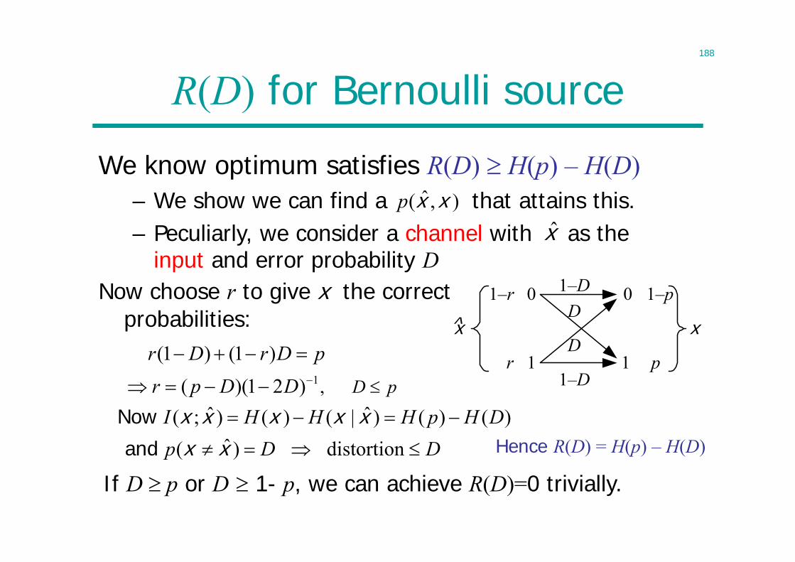
188
R(D) for Bernoulli source
We know optimum satisfies R(D) H(p) – H(D)– We show we can find a that attains this.),ˆ( xxp
x
D
0
1
0
1
xD
1–D
1–D
x
1–p
p
1–r
r
Now choose r to give x the correct probabilities:
Hence R(D) = H(p) – H(D)
– Peculiarly, we consider a channel with as the input and error probability D
ˆ ˆ( ; ) ( ) ( | ) ( ) ( )ˆ( ) distortion
I H H H p H Dp D D
x x x x xx x
Now
and
1,
(1 ) (1 )( )(1 2 ) D p
r D r D pr p D D
If D p or D 1- p, we can achieve R(D)=0 trivially.
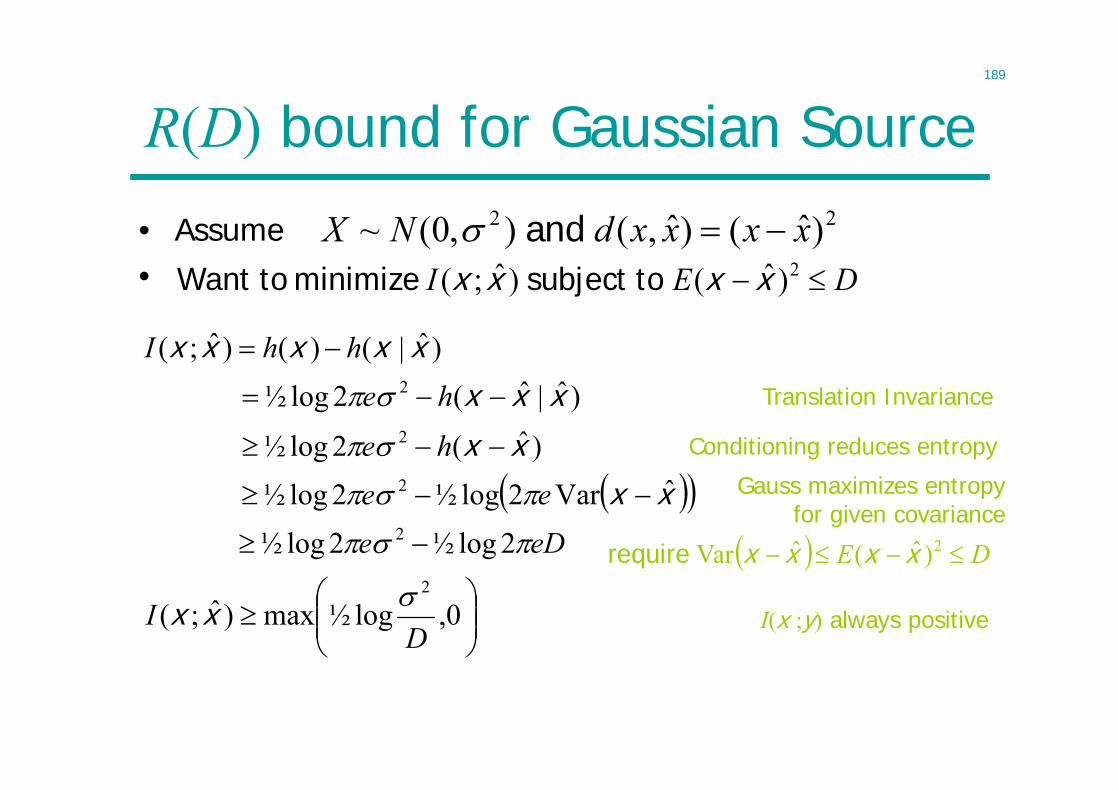
189
R(D) bound for Gaussian Source
• Assume 22 )ˆ()ˆ,(),0(~ xxxxdNX and
Translation Invariance
Conditioning reduces entropy
Gauss maximizes entropyfor given covariance
DE 2)ˆ(ˆVar xxxx require
DEI 2)ˆ()ˆ;( xxxx tosubject minimize toWant
I(x ;y) always positive
•
)ˆ|()()ˆ;( xxxxx hhI
)ˆ|ˆ(2log½ 2 xxx he
)ˆ(2log½ 2 xx he
xx ˆVar2log½2log½ 2 ee
eDe 2log½2log½ 2
0,log½max)ˆ;(
2
DI xx
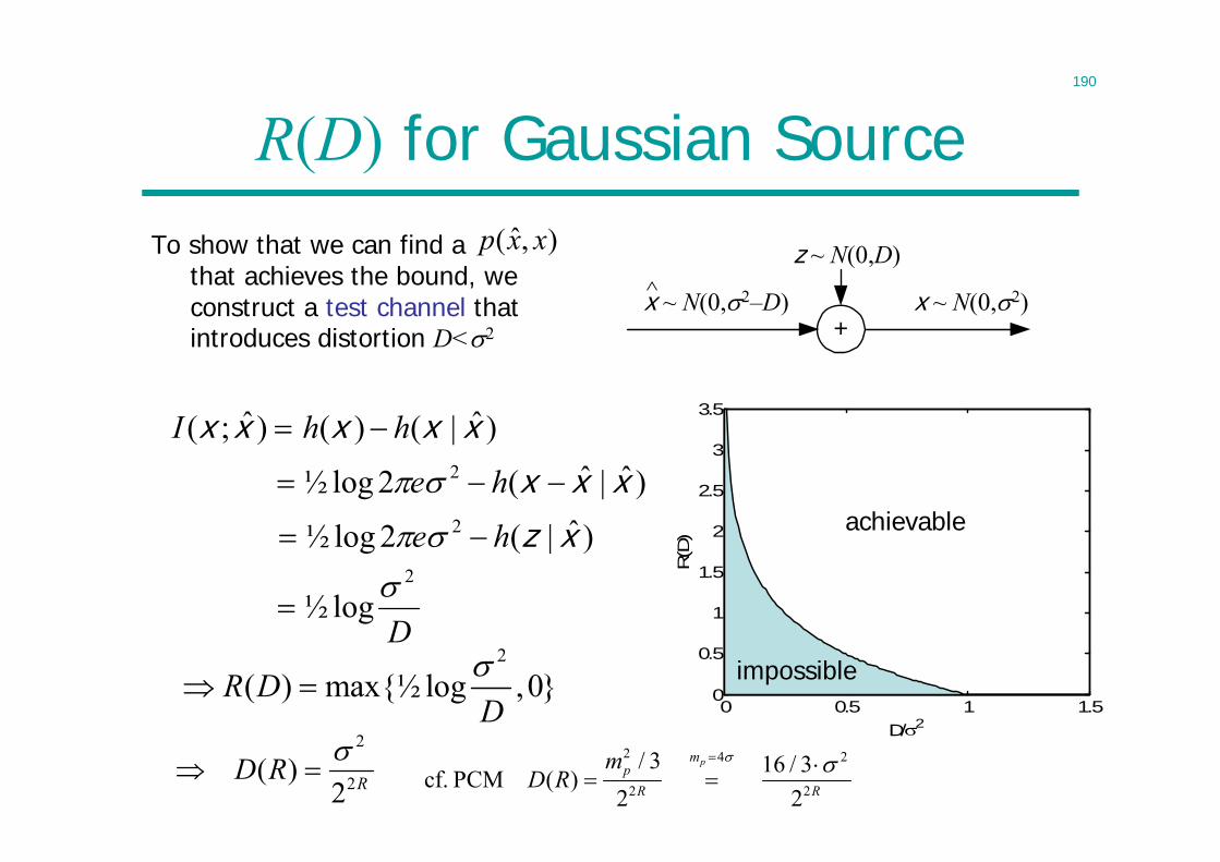
190
R(D) for Gaussian SourceTo show that we can find a
that achieves the bound, we construct a test channel that introduces distortion D<2 +
z ~ N(0,D)
x ~ N(0,2)x ~ N(0,2–D)^
0 0.5 1 1.50
0.5
1
1.5
2
2.5
3
3.5
D/2
R(D
) achievable
impossible
),ˆ( xxp
)ˆ|()()ˆ;( xxxxx hhI
)ˆ|ˆ(2log½ 2 xxx he
)ˆ|(2log½ 2 xzhe
D
2
log½
2
2( )2 RD R
2
( ) max{½ log ,0}R DD
2 24
2 2
/ 3 16 / 3cf. PCM ( )2 2
pmp
R R
mD R
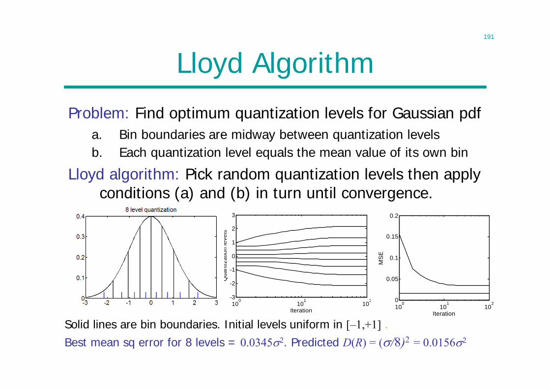
191
Lloyd Algorithm
Problem: Find optimum quantization levels for Gaussian pdf
100
101
102-3
-2
-1
0
1
2
3
Iteration
Qua
ntiz
atio
n le
vels
100
101
1020
0.05
0.1
0.15
0.2
Iteration
MS
E
Solid lines are bin boundaries. Initial levels uniform in [–1,+1] .
Lloyd algorithm: Pick random quantization levels then apply conditions (a) and (b) in turn until convergence.
b. Each quantization level equals the mean value of its own bina. Bin boundaries are midway between quantization levels
Best mean sq error for 8 levels = 0.03452. Predicted D(R) = (/8)2 = 0.01562
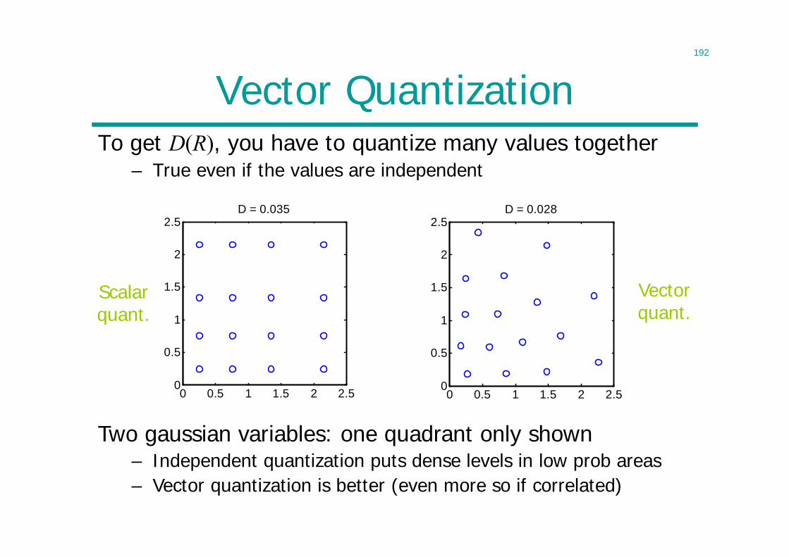
192
Vector QuantizationTo get D(R), you have to quantize many values together
– True even if the values are independent
0 0.5 1 1.5 2 2.50
0.5
1
1.5
2
2.5D = 0.035
Two gaussian variables: one quadrant only shown– Independent quantization puts dense levels in low prob areas– Vector quantization is better (even more so if correlated)
0 0.5 1 1.5 2 2.50
0.5
1
1.5
2
2.5D = 0.028
Scalar quant.
Vector quant.
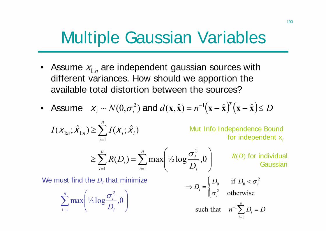
193
Multiple Gaussian Variables
• Assume x1:n are independent gaussian sources with different variances. How should we apportion the available total distortion between the sources?
DndN Tii xxxxxx ˆˆ)ˆ,(),0(~ 12 and x
Mut Info Independence Boundfor independent xi
R(D) for individual Gaussian
We must find the Di that minimize
n
i i
i
D1
2
0,log½max
• Assume
n
iiinn II
1:1:1 )ˆ;()ˆ;( xxxx
n
i i
in
ii D
DR1
2
10,log½max)(
20 02
1
1
if
otherwise
such that
ii
i
n
ii
D DD
n D D
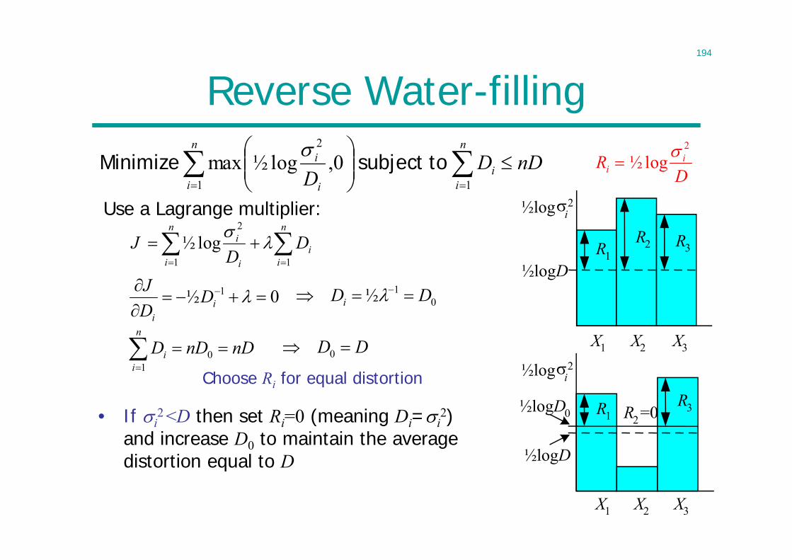
194
Reverse Water-filling
Use a Lagrange multiplier:
nDDD
n
ii
n
i i
i
11
2
0,log½max tosubject Minimize
½logi2
½logD
R3R2R1
X1 X2 X3
½logi2
½logD0R3R2=0R1
X3
½logD
X2X1
• If i2 <D then set Ri=0 (meaning Di=i
2) and increase D0 to maintain the average distortion equal to D
Choose Ri for equal distortion
n
ii
n
i i
i DD
J 11
2
log½
0½ 1 i
i
DDJ
01½ DDi
nDnDDn
ii
0
1
DD 0
DR i
i
2
log½
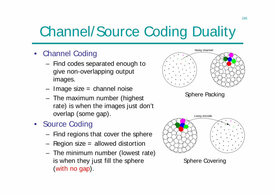
195
Channel/Source Coding DualityNoisy channel
• Channel Coding– Find codes separated enough to
give non-overlapping output images.
– Image size = channel noise– The maximum number (highest
rate) is when the images just don’t overlap (some gap). Lossy encode
Sphere Packing
Sphere Covering
• Source Coding– Find regions that cover the sphere– Region size = allowed distortion– The minimum number (lowest rate)
is when they just fill the sphere (with no gap).
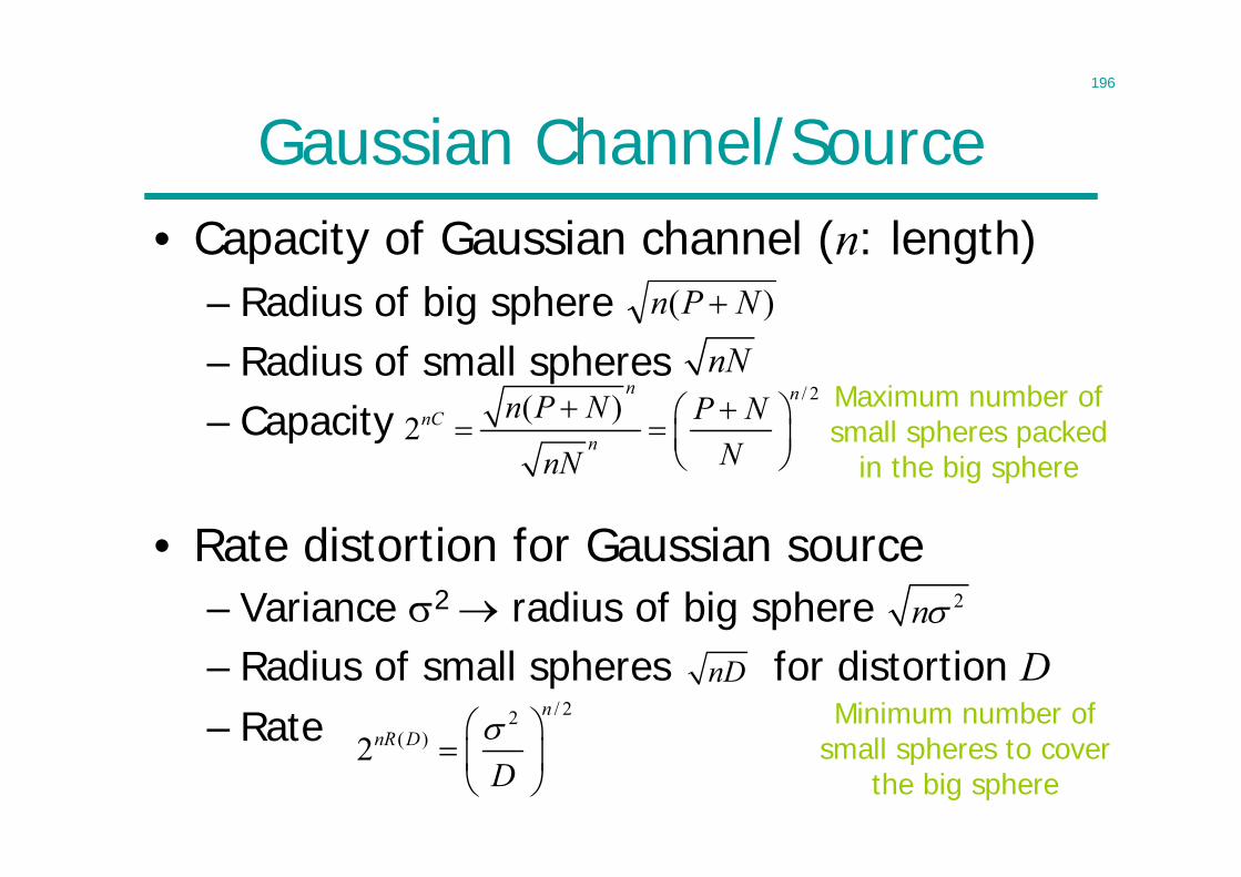
196
Gaussian Channel/Source• Capacity of Gaussian channel (n: length)
– Radius of big sphere– Radius of small spheres– Capacity
• Rate distortion for Gaussian source– Variance 2 radius of big sphere– Radius of small spheres for distortion D– Rate
)( NPn
nN/ 2( )
2n n
nCn
n P N P NNnN
2n
nD/ 22
( )2n
nR D
D
Maximum number of small spheres packed
in the big sphere
Minimum number of small spheres to cover
the big sphere
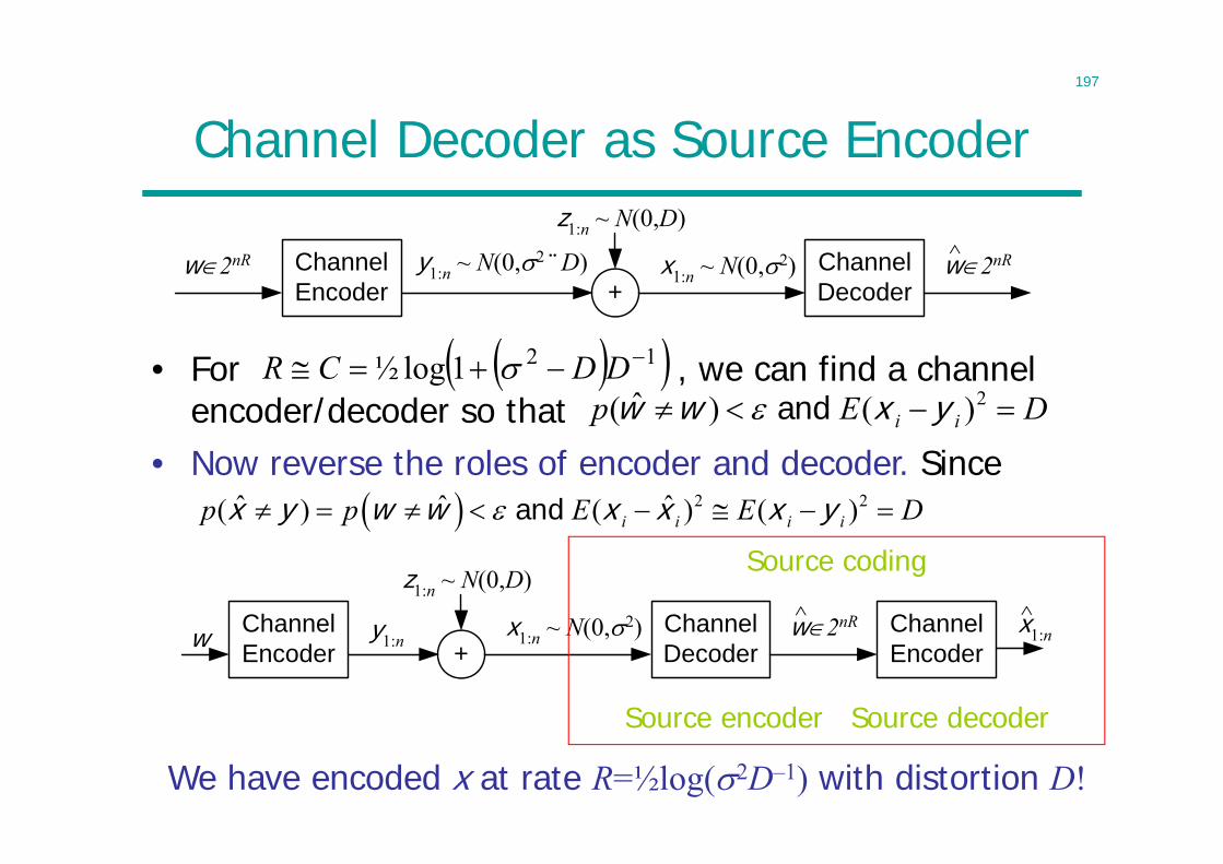
197
Channel Decoder as Source Encoder
• For , we can find a channel encoder/decoder so that
+
z1:n ~ N(0,D)
x1:n ~ N(0,2)ChannelEncoder
ChannelDecoder
w2nR w2nR^y1:n ~ N(0,2 ¨ D)
121log½ DDCR DEp ii 2)()ˆ( yxww and
2 2ˆ ˆ ˆ( ) ( ) ( )i i i ip p E E D x y w w x x x y and
We have encoded x at rate R=½log(2D–1) with distortion D!
• Now reverse the roles of encoder and decoder. Since
+
z1:n ~ N(0,D)
x1:n ~ N(0,2)ChannelEncoder
ChannelDecoderw w2nR^y1:n
ChannelEncoder
x1:n
Source coding
Source encoder Source decoder
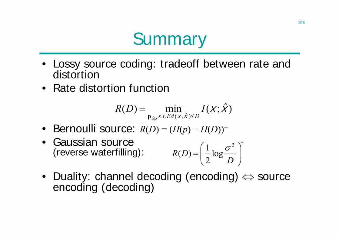
198
Summary• Lossy source coding: tradeoff between rate and
distortion• Rate distortion function
• Bernoulli source: R(D) = (H(p) – H(D))+
• Gaussian source(reverse waterfilling):
• Duality: channel decoding (encoding) source encoding (decoding)
)ˆ;(min)()ˆ,(..|ˆ
xxxxxx
IDRDEdts
p
21( ) log2
R DD
199
Nothing But Proof
• Proof of Rate Distortion Theorem– Converse: if the rate is less than R(D), then
distortion of any code is higher than D– Achievability: if the rate is higher than R(D),
then there exists a rate-R code which achieves distortion D
Quite technical!
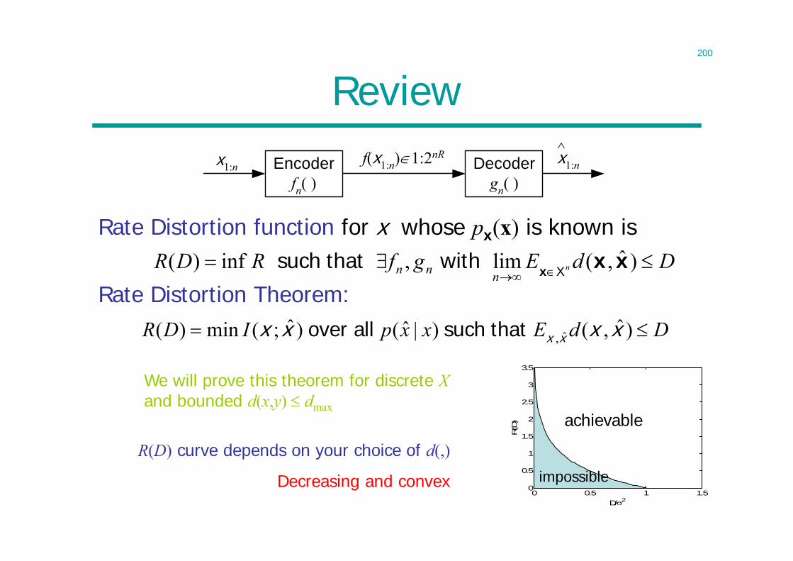
200
Review
Rate Distortion function for x whose px(x) is known is
x1:n Encoderfn( )
f(x1:n)1:2nRDecoder
gn( )x1:n^
DdEgfRDR nnnn
)ˆ,(lim,inf)( xxx X with that such
DdExxpIDR )ˆ,()|ˆ()ˆ;(min)( ˆ, xxxx xxthat such allover
0 0.5 1 1.50
0.5
1
1.5
2
2.5
3
3.5
D/2
R(D
) achievable
impossible
R(D) curve depends on your choice of d(,)
Decreasing and convex
We will prove this theorem for discrete Xand bounded d(x,y) dmax
Rate Distortion Theorem:
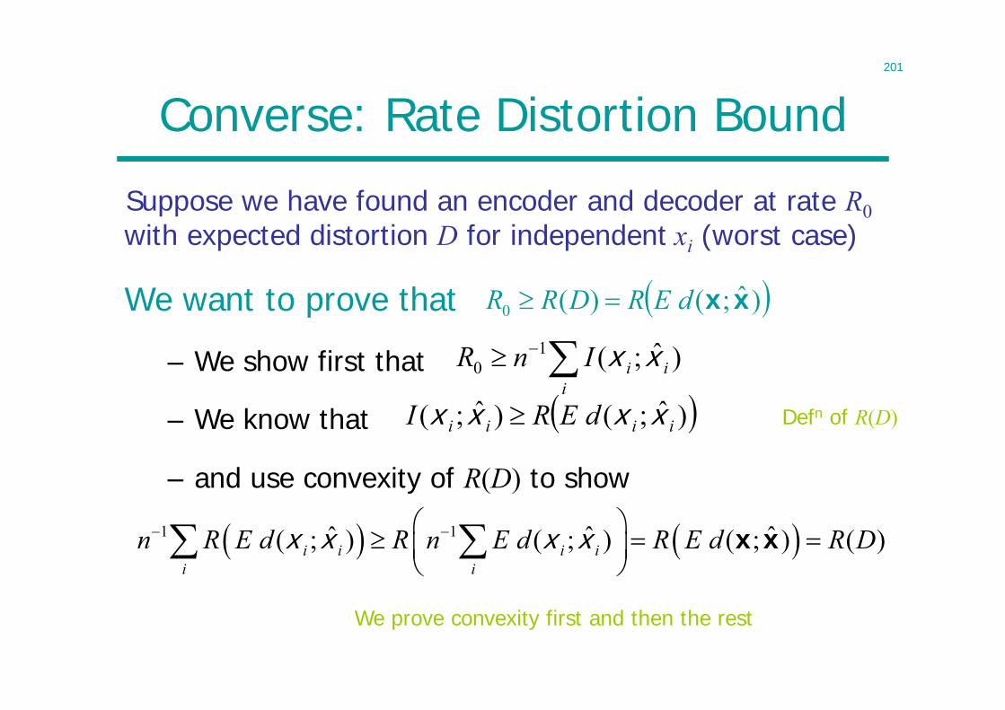
201
Converse: Rate Distortion Bound
We want to prove that
i
iiInR )ˆ;(10 xx
)ˆ;()ˆ;( iiii dERI xxxx
1 1ˆ ˆ ˆ( ; ) ( ; ) ( ; ) ( )i i i ii i
n R E d R n E d R E d R D
x x x x x x
We prove convexity first and then the rest
Defn of R(D)
Suppose we have found an encoder and decoder at rate R0with expected distortion D for independent xi (worst case)
)ˆ;()(0 xxdERDRR
– and use convexity of R(D) to show
– We know that
– We show first that
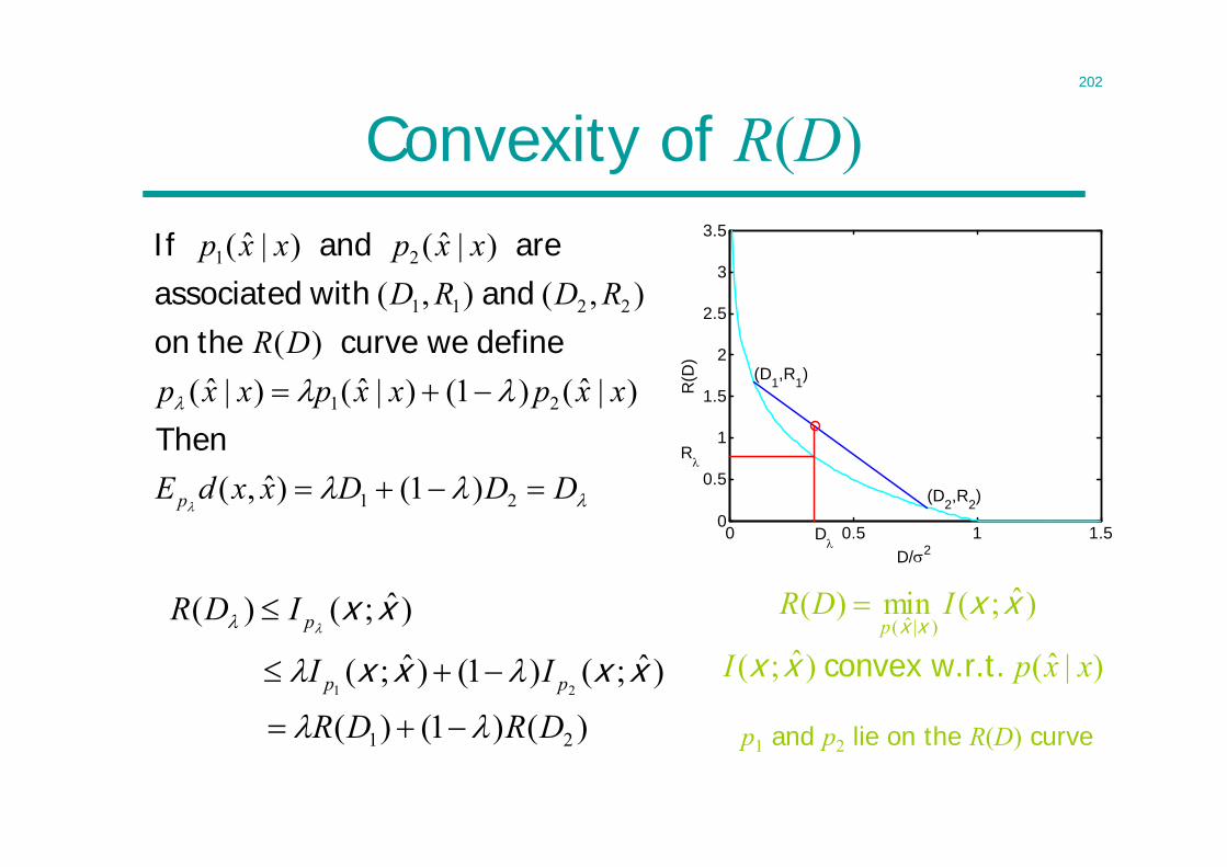
202
Convexity of R(D)
DDDxxdE
xxpxxpxxpDR
RDRDxxpxxp
p
21
21
2211
21
)1()ˆ,(
)|ˆ()1()|ˆ()|ˆ()(
),(),()|ˆ()|ˆ(
Then
define we curve the on and with associated
are and If
0 0.5 1 1.50
0.5
1
1.5
2
2.5
3
3.5
D/2
R(D
)
R
D
(D1,R1)
(D2,R2)
)|ˆ()ˆ;( xxpI w.r.t.convex xx
p1 and p2 lie on the R(D) curve
)ˆ;(min)()|ˆ(
xxxx
IDRp
)ˆ;()( xx pIDR
)ˆ;()1()ˆ;(21
xxxx pp II
)()1()( 21 DRDR
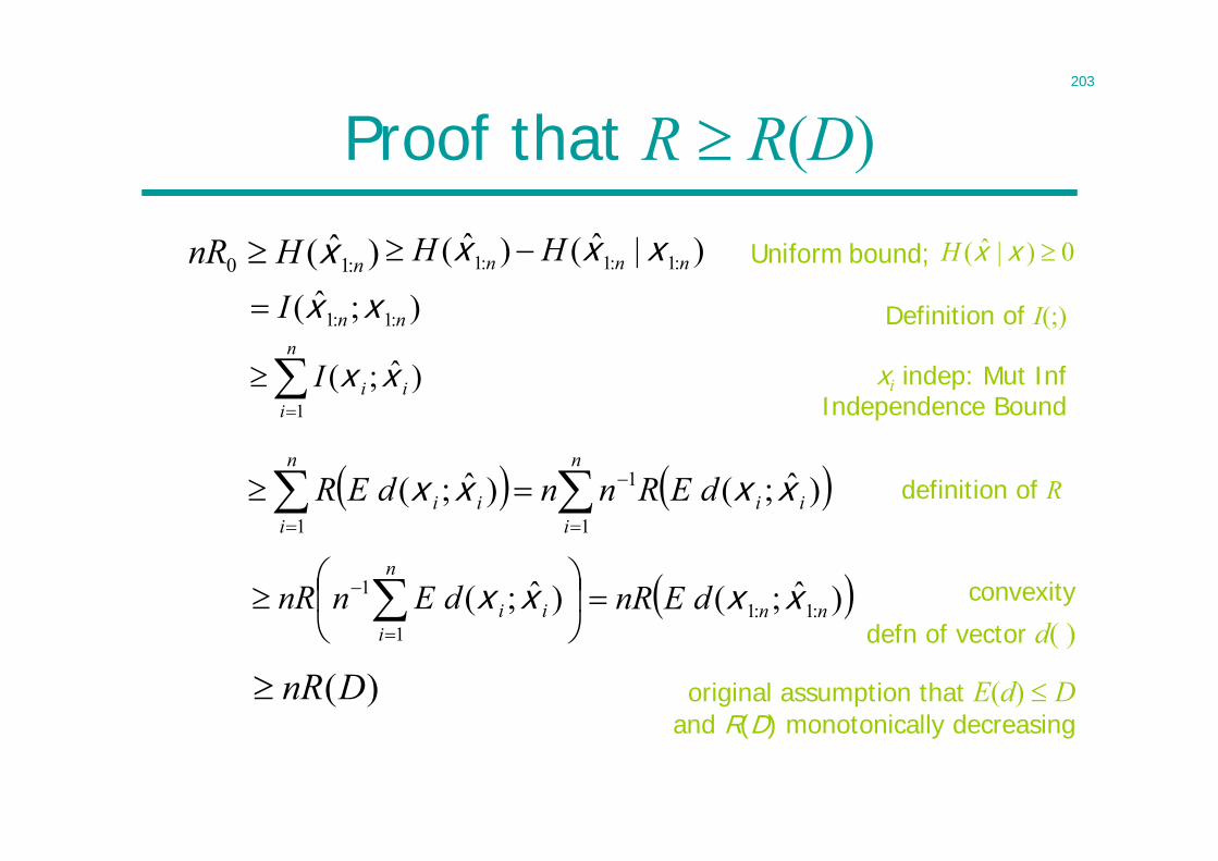
203
Proof that R R(D)
Definition of I(;)
bound; Uniform
xi indep: Mut Inf Independence Bound
definition of R
convexity
original assumption that E(d) Dand R(D) monotonically decreasing
)ˆ( :10 nHnR x 1: 1: 1:ˆ ˆ( ) ( | )n n nH H x x x
);ˆ( :1:1 nnI xx
n
iiiI
1
)ˆ;( xx
n
iii
n
iii dERnndER
1
1
1)ˆ;()ˆ;( xxxx
n
iiidEnnR
1
1 )ˆ;( xx )ˆ;( :1:1 nndEnR xx
)(DnR
ˆ( | ) 0H x x
defn of vector d( )
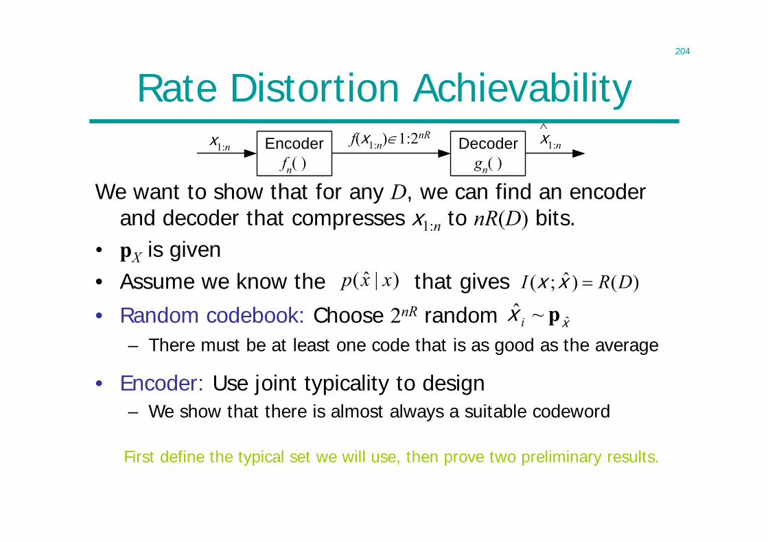
204
• Random codebook: Choose 2nR random– There must be at least one code that is as good as the average
Rate Distortion Achievability
We want to show that for any D, we can find an encoder and decoder that compresses x1:n to nR(D) bits.
• pX is given• Assume we know the that gives
x1:n Encoderfn( )
f(x1:n)1:2nRDecoder
gn( )x1:n^
)|ˆ( xxp )()ˆ;( DRI xx
xx ˆ~ˆ pi
First define the typical set we will use, then prove two preliminary results.
• Encoder: Use joint typicality to design– We show that there is almost always a suitable codeword
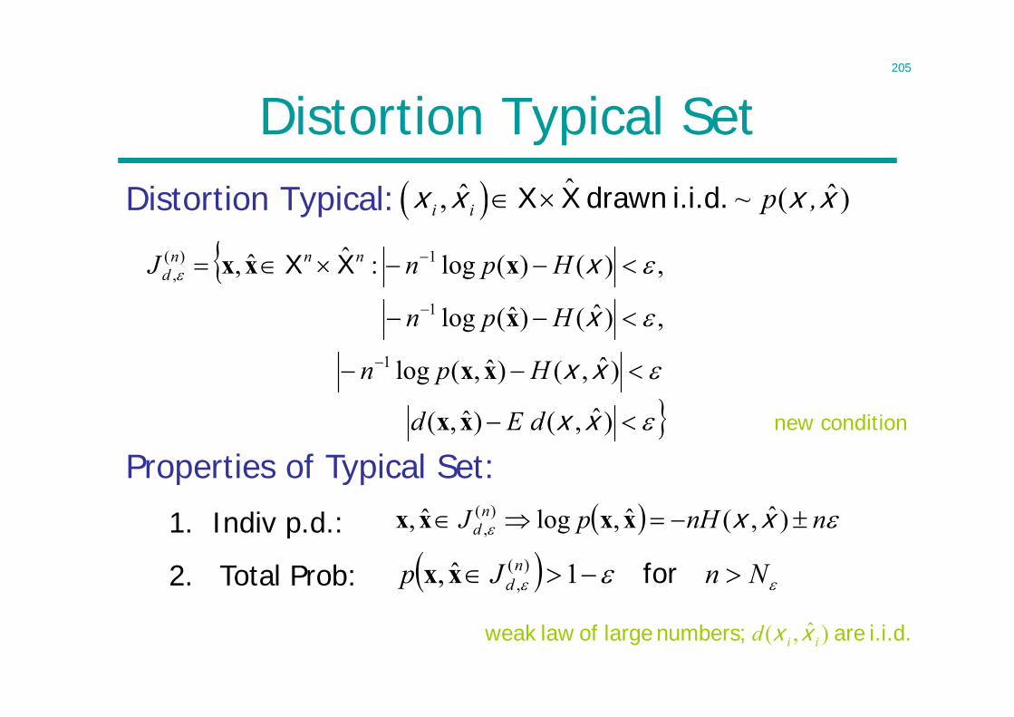
205
Distortion Typical SetDistortion Typical:
)ˆ,()ˆ,(
)ˆ,()ˆ,(log
,)ˆ()ˆ(log
,)()(log:ˆˆ,
1
1
1)(,
xx
xx
x
x
dEd
Hpn
Hpn
HpnJ nnnd
xx
xx
x
xxx XX
nnHpJ nd )ˆ,(ˆ,logˆ, )(
, xxxxxx
NnJp nd for1ˆ, )(
,xx
ˆˆ ˆ, ( )i i ~ p , x x x xX X drawn i.i.d.
new condition
i.i.d. are numbers; large of law weak )ˆ,( iid xx
2. Total Prob:
1. Indiv p.d.:
Properties of Typical Set:
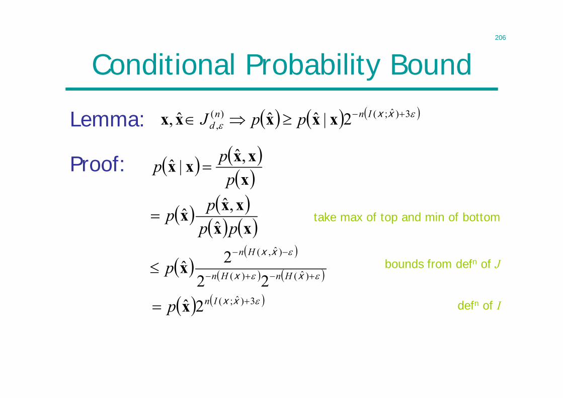
206
Conditional Probability Bound
Lemma:
3)ˆ;()(, 2|ˆˆˆ, xxInn
d ppJ xxxxx
bounds from defn of J
defn of I
take max of top and min of bottom
x
xxxxp
pp ,ˆ|ˆ
xx
xxxpp
ppˆ
,ˆˆ
)ˆ()(
)ˆ,(
222ˆ
xx
xx
HnHn
Hn
p x
3)ˆ;(2ˆ xxInp x
Proof:
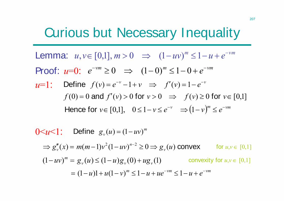
207
Curious but Necessary Inequality
Lemma: vmm euuvmvu 1)1(0],1,0[,vmmvm ee 01)01(0
convexity for u,v [0,1]
for u,v [0,1]
0<u<1:
u=1:Proof: u=0:
vv evfvevf 1)(1)( Define]1,0[0)(00)(0)0( vvfvvff for for and
vmmv evevv 110],1,0[for Hence
mv uvug )1()( Define
convex )(0)1()1()( 22 uguvvmmxg vn
v
)1()0()1()()1( vvvm ugguuguv
vmvmm euueuvuu 11)1(1)1(
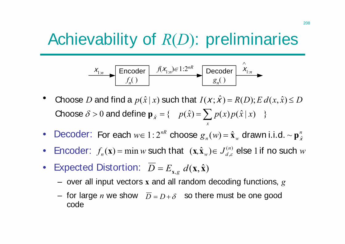
208
Achievability of R(D): preliminaries
•
x1:n Encoderfn( )
f(x1:n)1:2nRDecoder
gn( )x1:n^
})|ˆ()()ˆ({0)ˆ,();()ˆ;()|ˆ(
ˆ
xxxpxpxp
DxxdEDRIxxpD
x
xxp define and Choose
that such a find and Choose
nwn
nR wgw x~ˆ)(2:1 px i.i.d. drawn choose eachFor
w J, wf ndwn such no if else that such 1)ˆ(min)( )(
, xxx
)ˆ,(, xxx dED g
DD– for large n we show so there must be one good code
– over all input vectors x and all random decoding functions, g
• Expected Distortion:
• Encoder:
• Decoder:
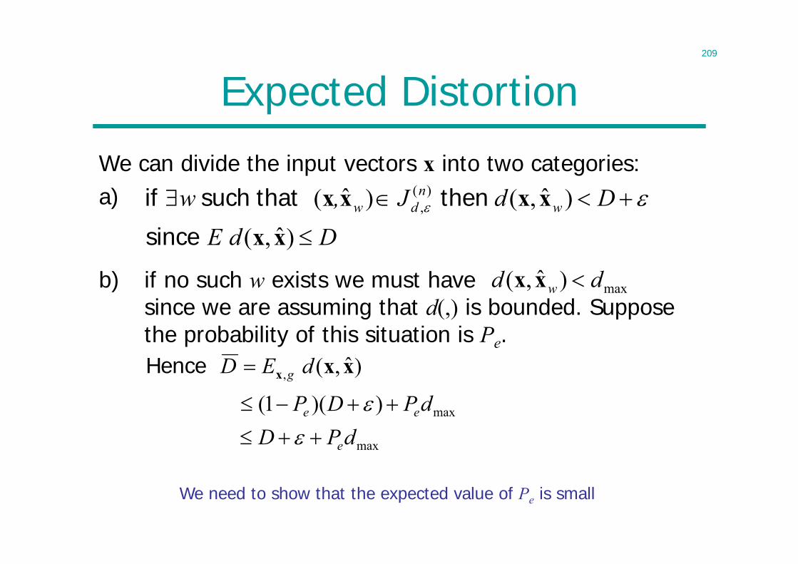
209
Expected Distortion
We can divide the input vectors x into two categories:
DdEDdJ, w w
ndw
)ˆ,()ˆ,()ˆ( )(
,
xxxxxx
since
then that such if
We need to show that the expected value of Pe is small
b) if no such w exists we must have since we are assuming that d(,) is bounded. Suppose the probability of this situation is Pe.
a)
)ˆ,(, xxx dED g Hence
max))(1( dPDP ee
maxdPD e
max)ˆ,( dd w xx
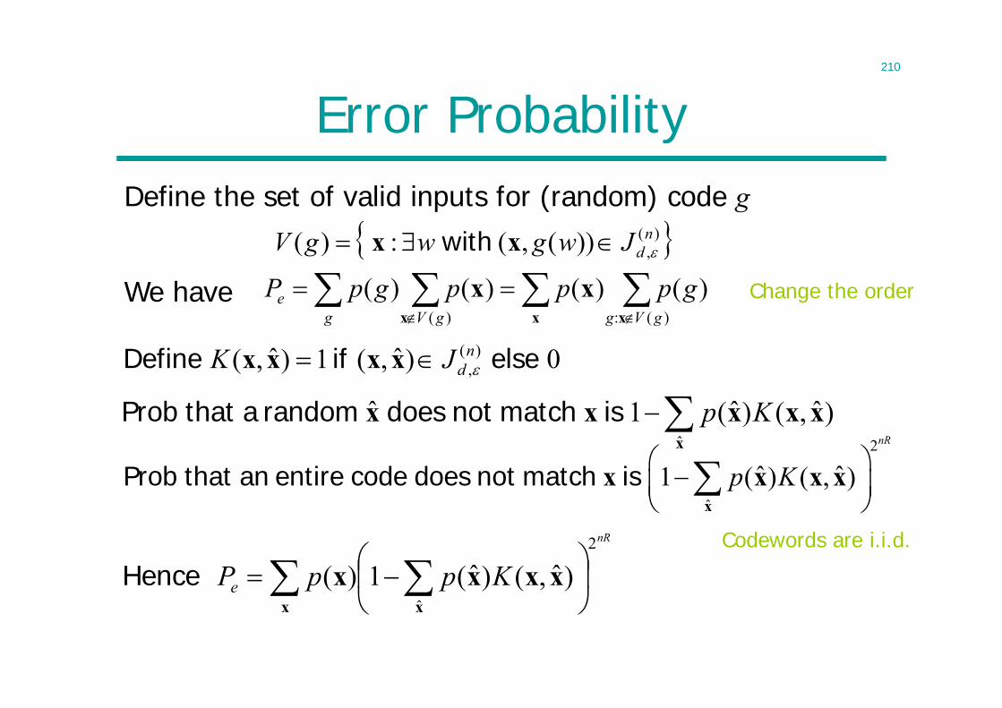
210
Error ProbabilityDefine the set of valid inputs for (random) code g
0)ˆ,(1)ˆ,( )(, else if Define n
dJK xxxx
x xx
xx)(:)(
)()()()(gVgg gV
e gpppgpP
)(,))(,(:)( n
dJwgwgV xx with
x
xxxxxˆ
)ˆ,()ˆ(1ˆ Kp is matchnot does random athat Prob2
ˆ
ˆ ˆ1 ( ) ( , )nR
p K
Prob that an entire code does not match is x
x x x x
x x
xxxxnR
KppPe
2
ˆ)ˆ,()ˆ(1)( Hence
We have Change the order
Codewords are i.i.d.
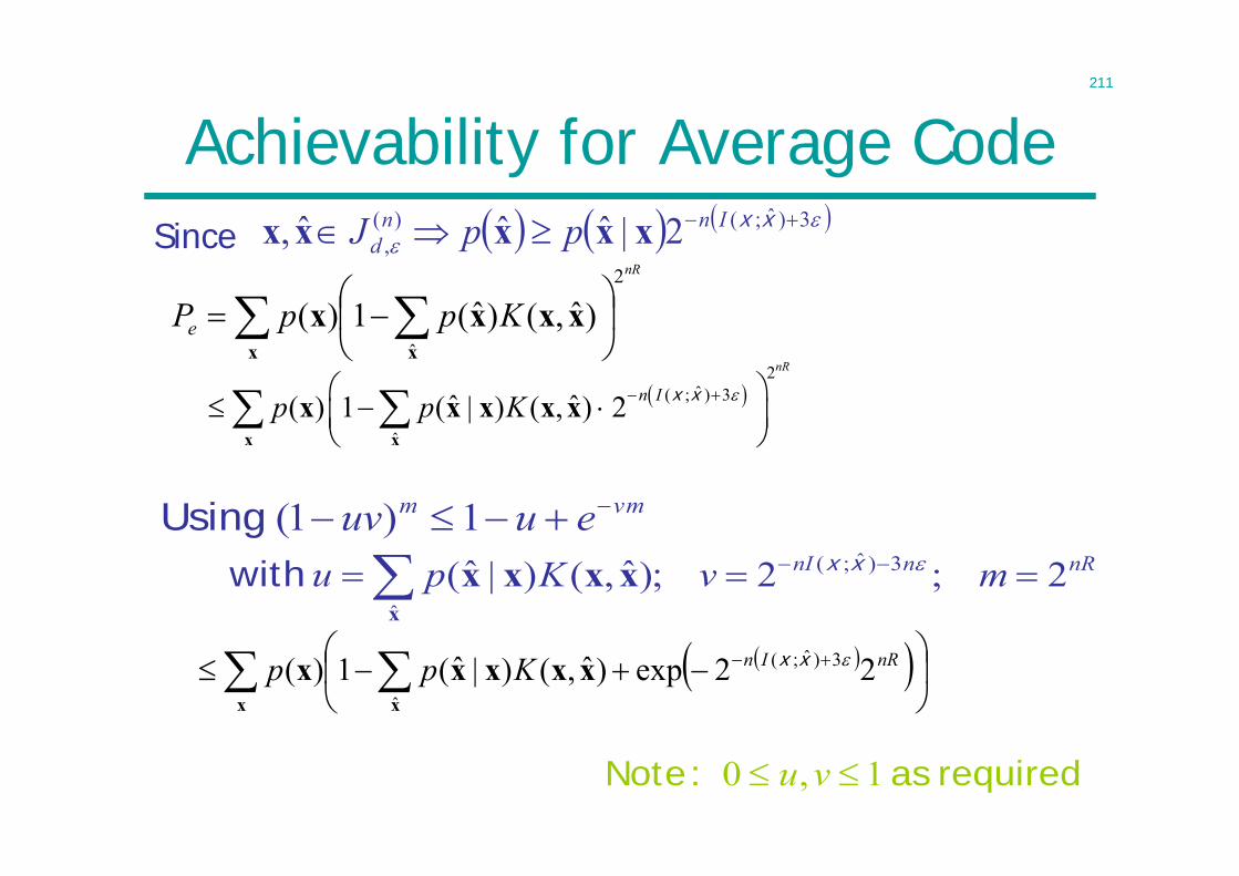
211
Achievability for Average CodeSince
3)ˆ;()(
, 2|ˆˆˆ, xxInnd ppJ xxxxx
vmm euuv 1)1( Using
2
ˆ( ; ) 3
ˆ
ˆ ˆ( ) 1 ( | ) ( , ) 2nR
n Ip p K
x x
x x x x x x x
x x
xxxxnR
KppPe
2
ˆ)ˆ,()ˆ(1)(
x xxxxxx
ˆ
3)ˆ;( 22exp)ˆ,()|ˆ(1)( nRInKpp xx
nRnnI mvKpu 2;2;)ˆ,()|ˆ( 3)ˆ;(
ˆ xx
xxxxx with
required as :Note 1,0 vu
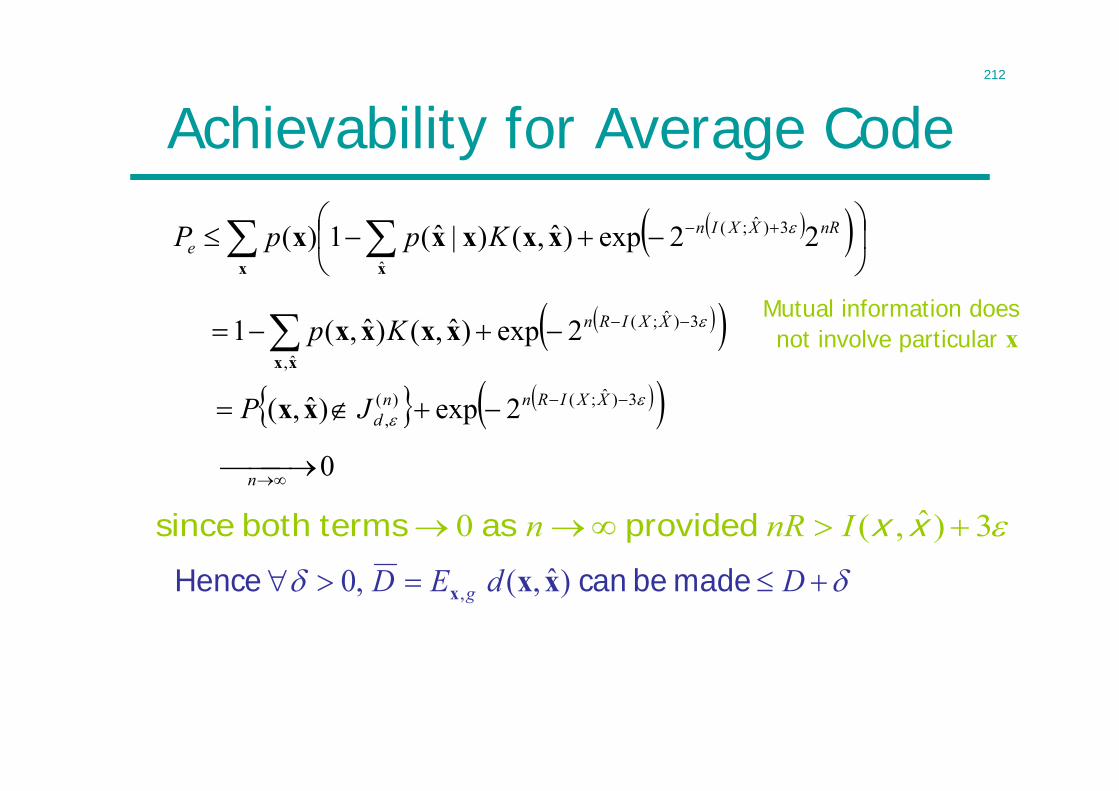
212
Achievability for Average Code
DdED g made be can Hence )ˆ,(,0 , xxx
x xxxxxx
ˆ
3)ˆ;( 22exp)ˆ,()|ˆ(1)( nRXXIne KppP
3)ˆ;(
ˆ,2exp)ˆ,()ˆ,(1 XXIRnKp
xxxxxx
Mutual information does not involve particular x
3)ˆ;()(, 2exp)ˆ,( XXIRnn
dJP xx
ˆ0 ( , ) 3 n nR I x xsince both terms as provided
0 n
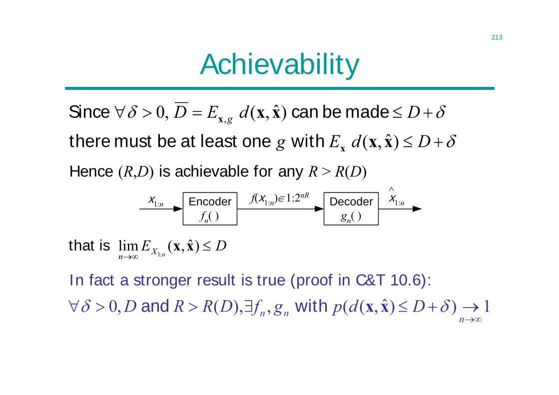
213
Achievability
Hence (R,D) is achievable for any R > R(D)
DdEg
DdED g
with oneleast at bemust there
made be can Since
)ˆ,(
)ˆ,(,0 ,
xx
xx
x
x
DEnXn
)ˆ,(lim:1
xx isthat
x1:n Encoderfn( )
f(x1:n)1:2nRDecoder
gn( )x1:n^
In fact a stronger result is true (proof in C&T 10.6):
1))ˆ,((,),(,0
nnn DdpgfDRRD xx with and
214
Lecture 16
• Introduction to network information theory
• Multiple access• Distributed source coding
215
Network Information Theory• System with many senders and receivers• New elements: interference, cooperation,
competition, relay, feedback…• Problem: decide whether or not the sources can
be transmitted over the channel– Distributed source coding– Distributed communication– The general problem has not yet been solved, so we
consider various special cases
• Results are presented without proof (can be done using mutual information, joint AEP)
216
Implications to Network Design• Examples of large information networks
– Computer networks– Satellite networks– Telephone networks
• A complete theory of network communications would have wide implications for the design of communication and computer networks
• Examples– CDMA (code-division multiple access): mobile phone
network– Network coding: significant capacity gain compared to
routing-based networks
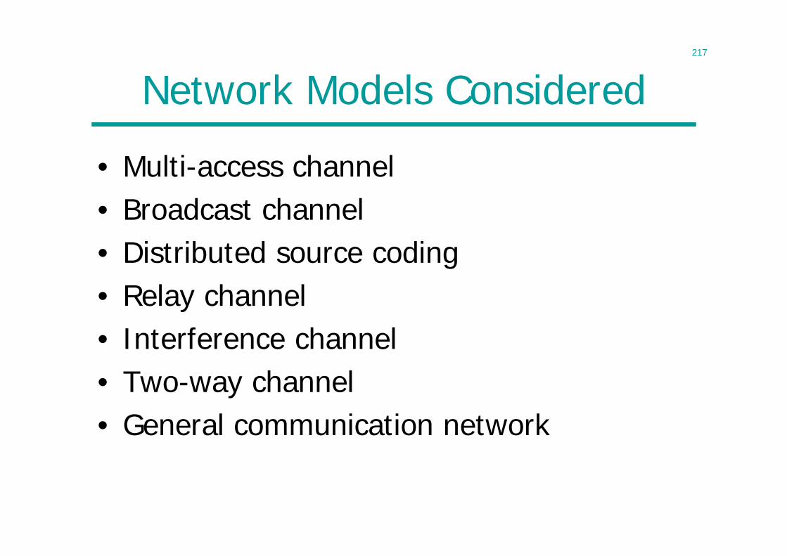
217
Network Models Considered
• Multi-access channel• Broadcast channel• Distributed source coding • Relay channel• Interference channel• Two-way channel• General communication network
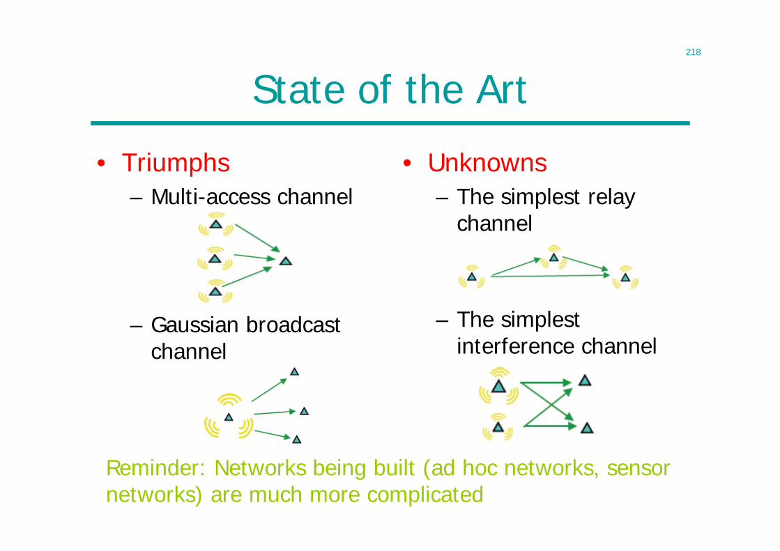
218
State of the Art
• Triumphs– Multi-access channel
– Gaussian broadcast channel
• Unknowns– The simplest relay
channel
– The simplest interference channel
Reminder: Networks being built (ad hoc networks, sensor networks) are much more complicated
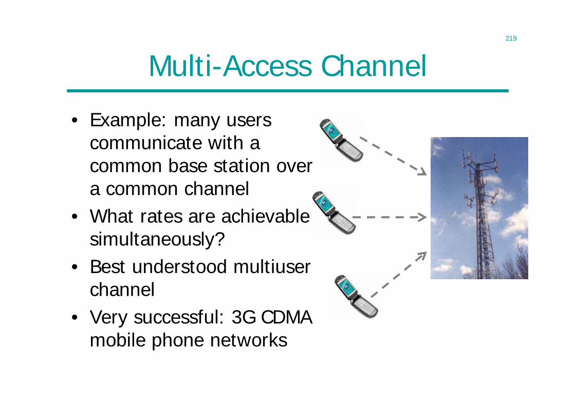
219
Multi-Access Channel
• Example: many users communicate with a common base station over a common channel
• What rates are achievable simultaneously?
• Best understood multiuser channel
• Very successful: 3G CDMA mobile phone networks
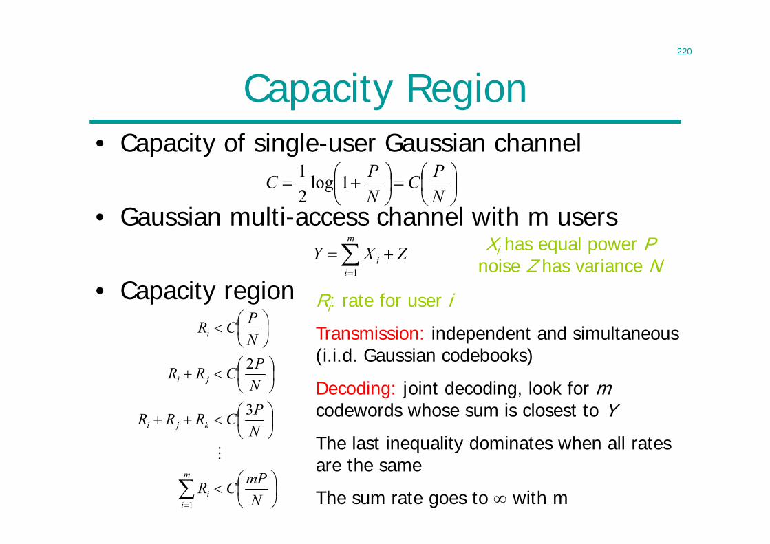
220
Capacity Region• Capacity of single-user Gaussian channel
• Gaussian multi-access channel with m users
• Capacity region
NPC
NPC 1log
21
m
ii ZXY
1
N
mPCR
NPCRRR
NPCRR
NPCR
m
ii
kji
ji
i
1
3
2
Xi has equal power Pnoise Z has variance N
Ri: rate for user i
Transmission: independent and simultaneous (i.i.d. Gaussian codebooks)
Decoding: joint decoding, look for mcodewords whose sum is closest to Y
The last inequality dominates when all rates are the same
The sum rate goes to with m
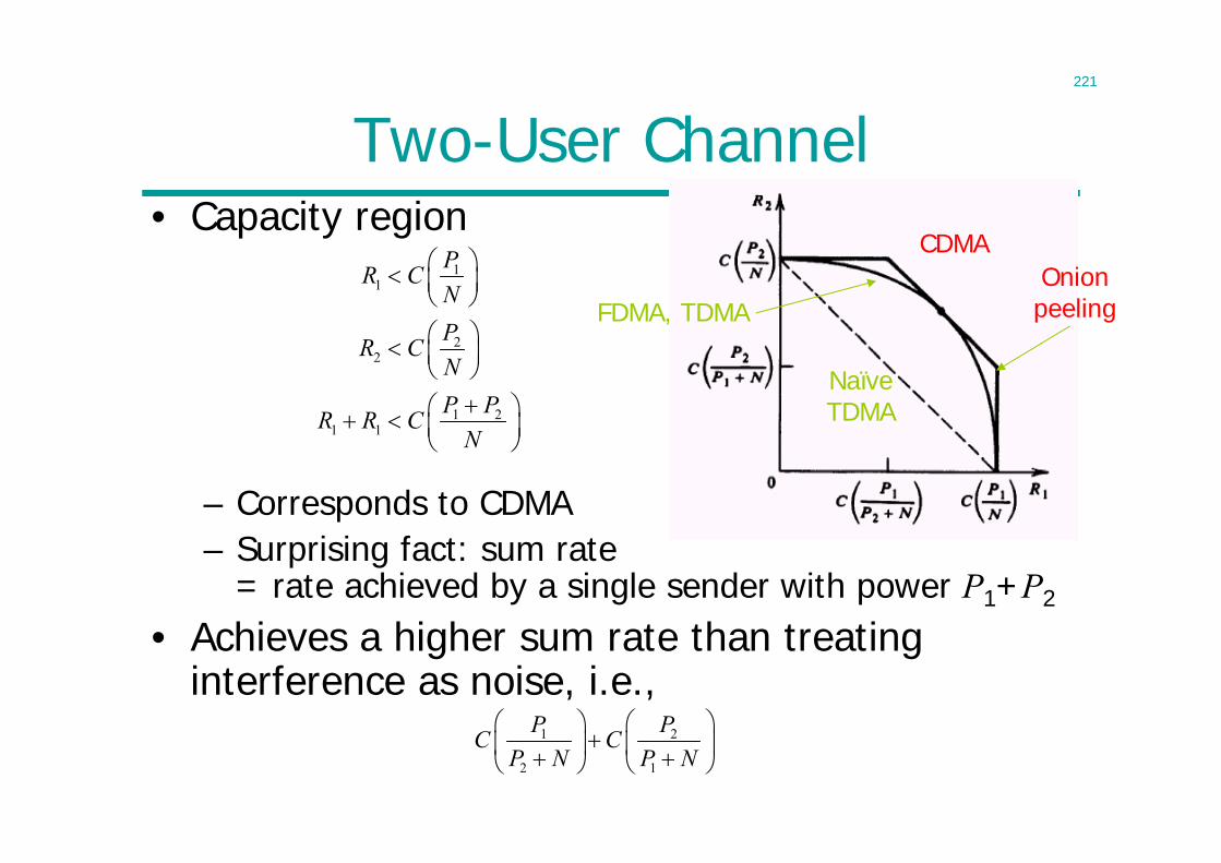
221
Two-User Channel• Capacity region
– Corresponds to CDMA– Surprising fact: sum rate
= rate achieved by a single sender with power P1+P2
• Achieves a higher sum rate than treating interference as noise, i.e.,
11
22
1 21 1
PR CNPR CNP PR R C
N
Naïve TDMA
CDMA
FDMA, TDMA
1 2
2 1
P PC CP N P N
Onion peeling
222
Onion Peeling• Interpretation of corner point: onion-peeling
– First stage: decoder user 2, considering user 1 as noise– Second stage: subtract out user 2, decoder user 1
• In fact, it can achieve the entire capacity region– Any rate-pairs between two corner points achievable by time-
sharing
• Its technical term is successive interference cancelation (SIC)– Removes the need for joint decoding– Uses a sequence of single-user decoders
• SIC is implemented in the uplink of CDMA 2000 EV-DO (evolution-data optimized)– Increases throughput by about 65%
223
Comparison with TDMA and FDMA• FDMA (frequency-division multiple access)
• TDMA (time-division multiple access)– Each user is allotted a time slot, transmits and other
users remain silent– Naïve TDMA: dashed line– Can do better while still maintaining the same
average power constraint; the same capacity region as FDMA
• CDMA capacity region is larger– But needs a more complex decoder
11 1
0 1
22 2
0 2
log 1
log 1
PR WN W
PR WN W
Total bandwidth W = W1 + W2
Varying W1 and W2 tracing out the curve in the figure
224
Distributed Source Coding
• Associate with nodes are sources that are generally dependent
• How do we take advantage of the dependence to reduce the amount of information transmitted?
• Consider the special case where channels are noiseless and without interference
• Finding the set of rates associate with each source such that all required sources can be decoded at destination
• Data compression dual to multi-access channel
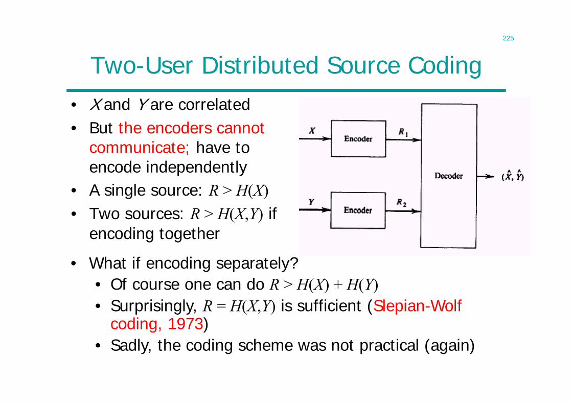
225
Two-User Distributed Source Coding• X and Y are correlated• But the encoders cannot
communicate; have to encode independently
• A single source: R > H(X)• Two sources: R > H(X,Y) if
encoding together
• What if encoding separately?• Of course one can do R > H(X) + H(Y)• Surprisingly, R = H(X,Y) is sufficient (Slepian-Wolf
coding, 1973)• Sadly, the coding scheme was not practical (again)
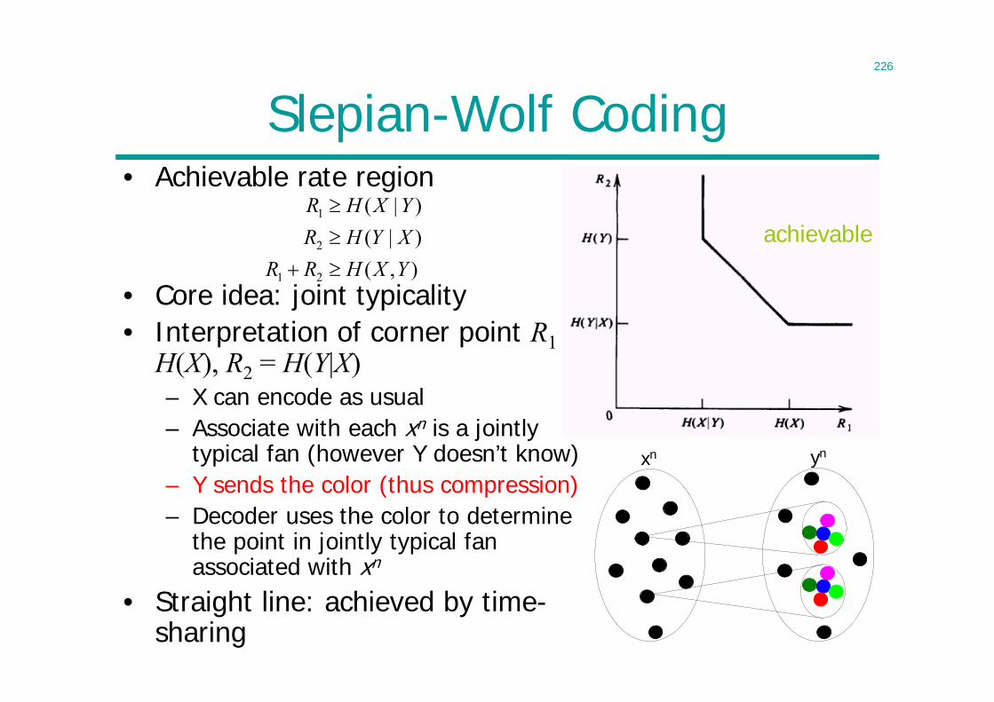
226
Slepian-Wolf Coding• Achievable rate region
• Core idea: joint typicality• Interpretation of corner point R1 =
H(X), R2 = H(Y|X)– X can encode as usual– Associate with each xn is a jointly
typical fan (however Y doesn’t know)– Y sends the color (thus compression)– Decoder uses the color to determine
the point in jointly typical fan associated with xn
• Straight line: achieved by time-sharing
),()|()|(
21
2
1
YXHRRXYHRYXHR
achievable
xn yn
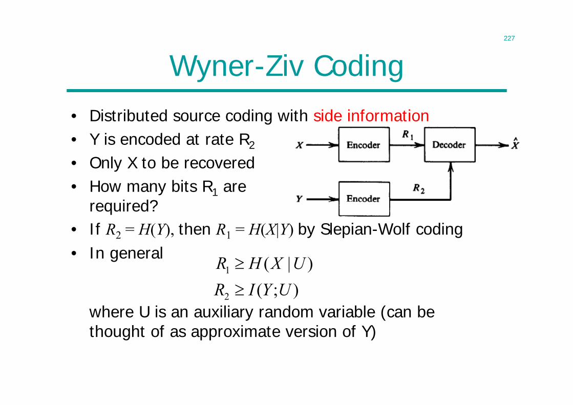
227
Wyner-Ziv Coding• Distributed source coding with side information• Y is encoded at rate R2
• Only X to be recovered• How many bits R1 are
required?• If R2 = H(Y), then R1 = H(X|Y) by Slepian-Wolf coding• In general
where U is an auxiliary random variable (can be thought of as approximate version of Y)
1
2
( | )( ; )
R H X UR I Y U
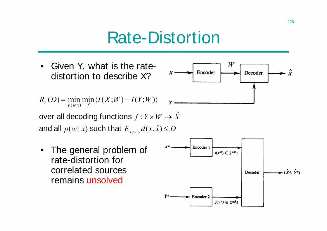
228
Rate-Distortion• Given Y, what is the rate-
distortion to describe X?
• The general problem of rate-distortion for correlated sources remains unsolved
DdExxpIDR )ˆ,()|ˆ()ˆ;(min)( ˆ, xxxx xxthat such allover
( | )
, ,
( ) min min{ ( ; ) ( ; )}
ˆ:ˆ( | ) ( , )
Y p w x f
x w y
R D I X W I Y W
f Y W Xp w x E d x x D
over all decoding functions and all such that
W
229
Lecture 17
• Network information theory – II– Broadcast– Relay– Interference channel– Two-way channel– Comments on general communication
networks
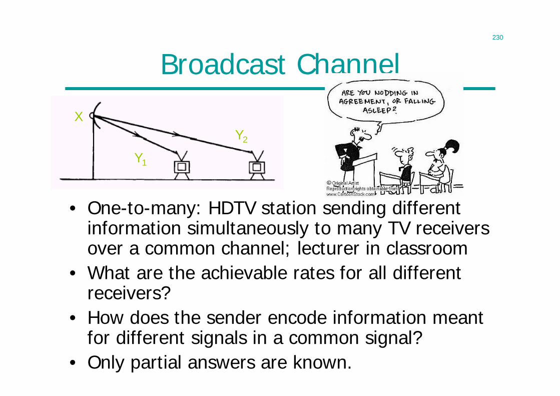
230
Broadcast Channel
• One-to-many: HDTV station sending different information simultaneously to many TV receivers over a common channel; lecturer in classroom
• What are the achievable rates for all different receivers?
• How does the sender encode information meant for different signals in a common signal?
• Only partial answers are known.
X
Y1
Y2
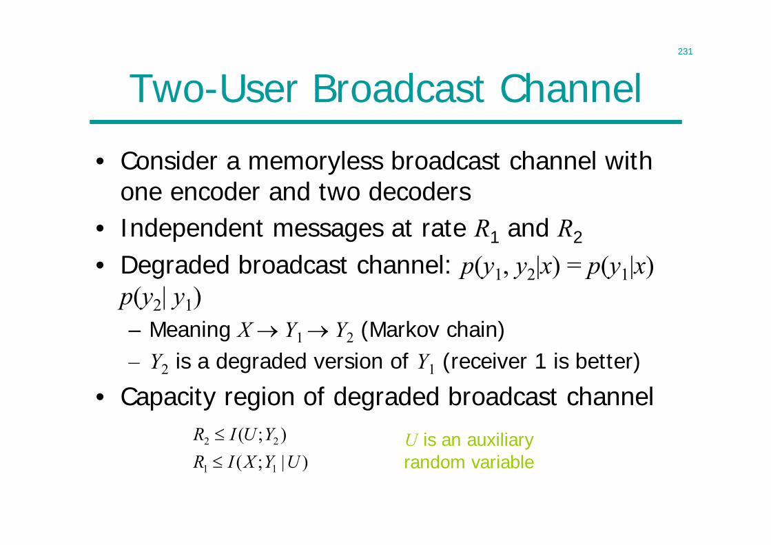
231
Two-User Broadcast Channel
• Consider a memoryless broadcast channel with one encoder and two decoders
• Independent messages at rate R1 and R2
• Degraded broadcast channel: p(y1, y2|x) = p(y1|x) p(y2| y1)– Meaning X Y1 Y2 (Markov chain)– Y2 is a degraded version of Y1 (receiver 1 is better)
• Capacity region of degraded broadcast channel
)|;();(
11
22
UYXIRYUIR
U is an auxiliary
random variable
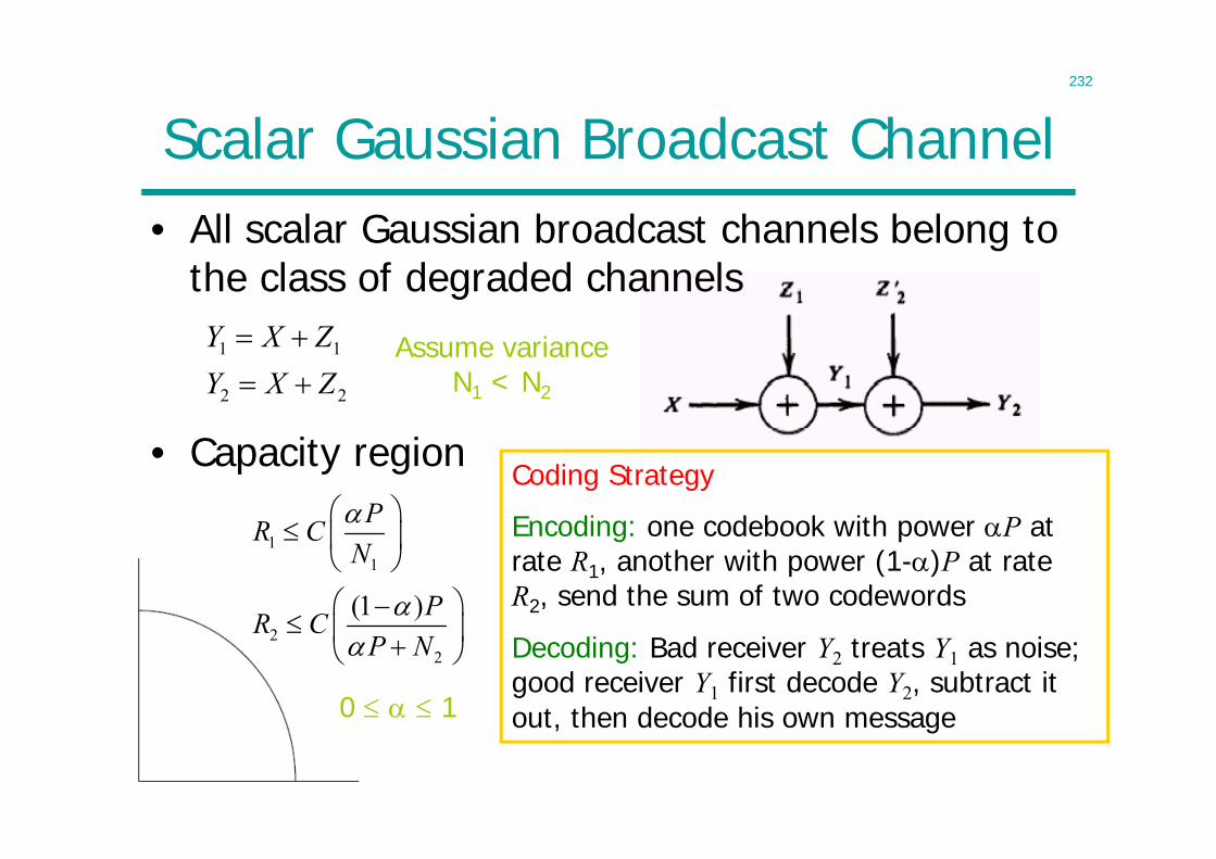
232
Scalar Gaussian Broadcast Channel• All scalar Gaussian broadcast channels belong to
the class of degraded channels
• Capacity region
11
22
(1 )
PR CN
PR CP N
22
11
ZXYZXY
Assume variance
N1 < N2
0 1
Coding Strategy
Encoding: one codebook with power P at rate R1, another with power (1-)P at rate R2, send the sum of two codewords
Decoding: Bad receiver Y2 treats Y1 as noise; good receiver Y1 first decode Y2, subtract it out, then decode his own message
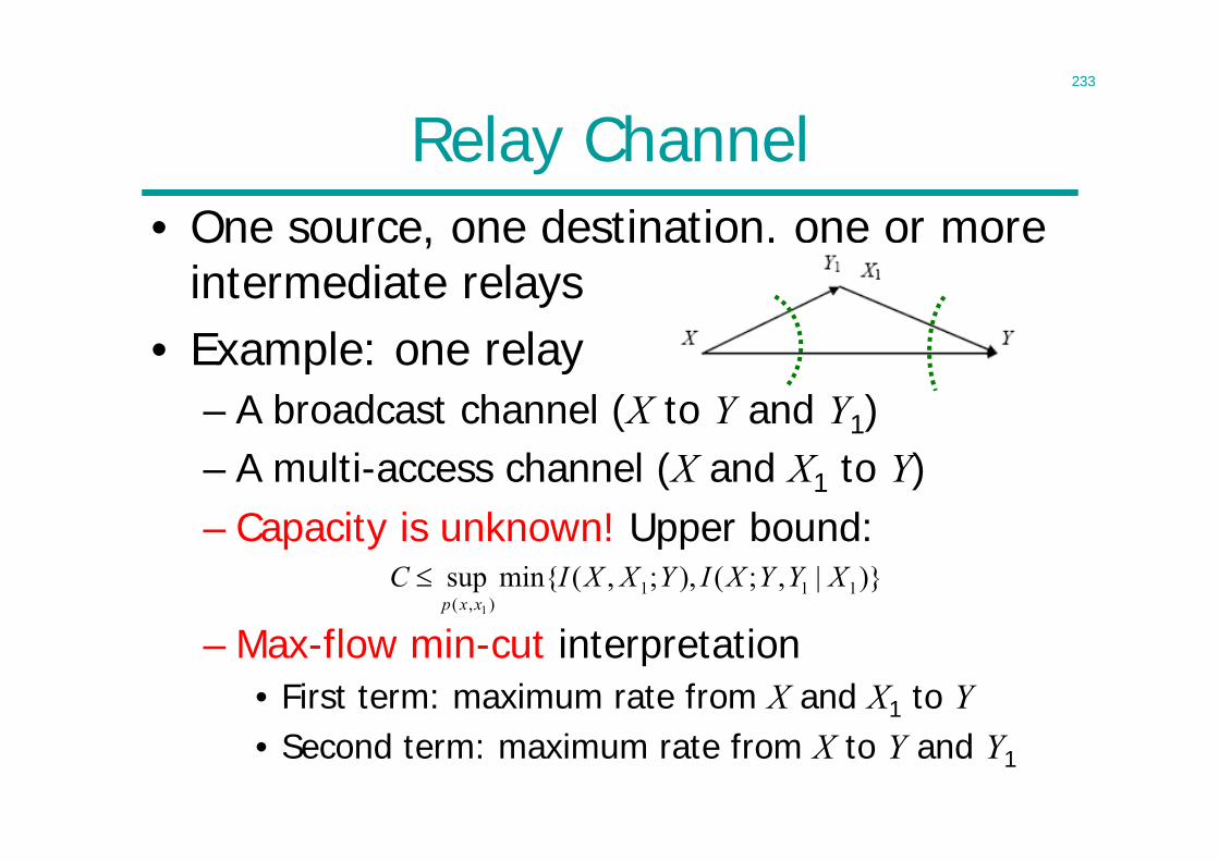
233
Relay Channel• One source, one destination, one or more
intermediate relays• Example: one relay
– A broadcast channel (X to Y and Y1)– A multi-access channel (X and X1 to Y)– Capacity is unknown! Upper bound:
– Max-flow min-cut interpretation• First term: maximum rate from X and X1 to Y• Second term: maximum rate from X to Y and Y1
)}|,;(),;,(min{sup 111),( 1
XYYXIYXXICxxp
234
Degraded Relay Channel
• In general, the max-flow min-cut bound cannot be achieved
• Reason– Interference– What for the relay to forward?– How to forward?
• Capacity is known for degraded relay channel (i.e, Y is a degradation of Y1, or relay is better than receiver), i.e., the upper bound is achieved
1
1 1 1( , )sup min{ ( , ; ), ( ; , | )}p x x
C I X X Y I X Y Y X
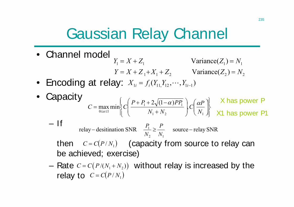
235
Gaussian Relay Channel• Channel model
• Encoding at relay:• Capacity
– If
then (capacity from source to relay can be achieved; exercise)
– Rate without relay is increased by the relay to
1 1 1 1
1 1 2 2 2
Variance( )Variance( )
Y X Z Z NY X Z X Z Z N
),,( 1112,111 iii YYYfX
121
11
10,
)1(2minmax
NPC
NNPPPP
CC
X has power P
X1 has power P1
SNRrelaysourceSNRondesitinatirelay12
1 NP
NP
1/ NPCC
1 2/( )C C P N N 1/ NPCC
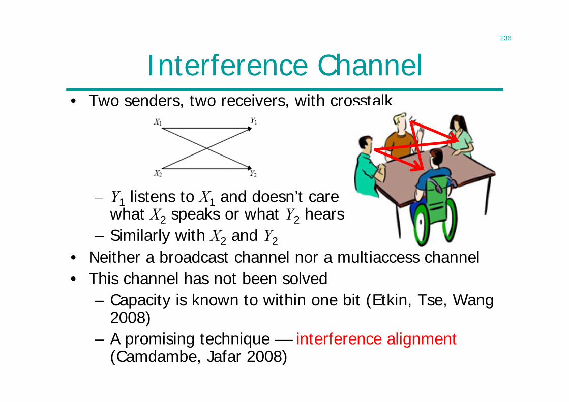
236
Interference Channel• Two senders, two receivers, with crosstalk
– Y1 listens to X1 and doesn’t care what X2 speaks or what Y2 hears
– Similarly with X2 and Y2
• Neither a broadcast channel nor a multiaccess channel• This channel has not been solved
– Capacity is known to within one bit (Etkin, Tse, Wang 2008)
– A promising technique interference alignment(Camdambe, Jafar 2008)
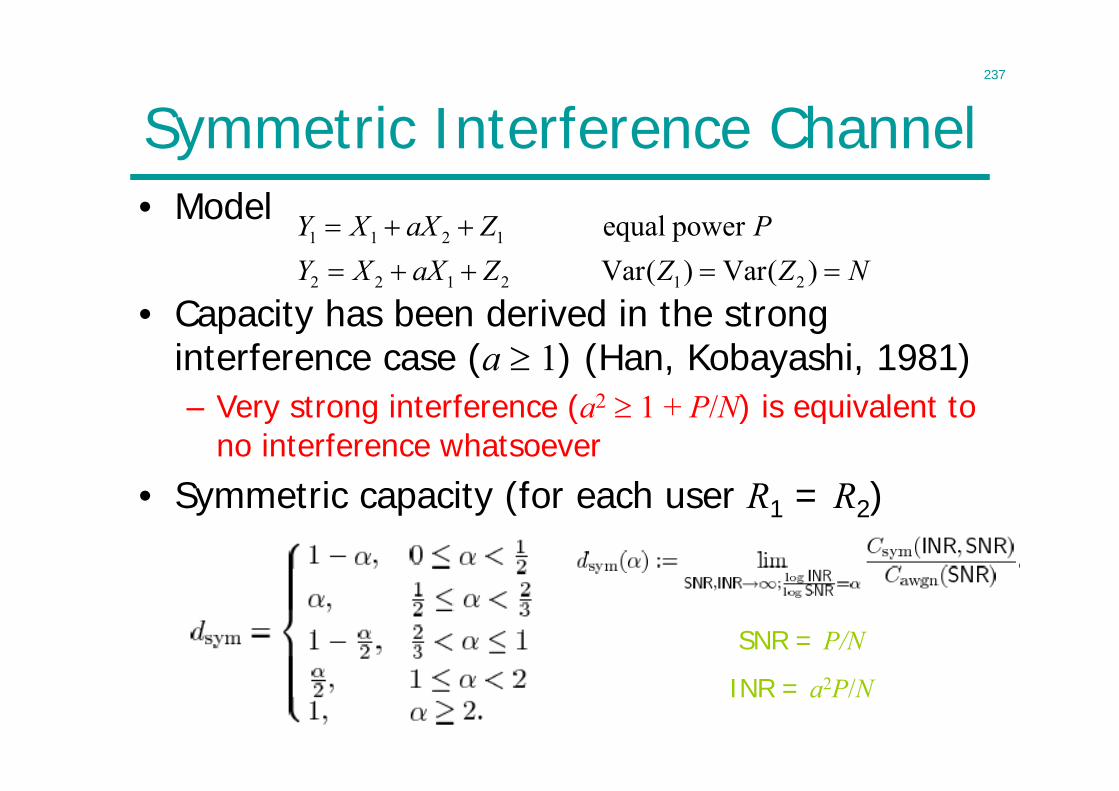
237
Symmetric Interference Channel• Model
• Capacity has been derived in the strong interference case (a 1) (Han, Kobayashi, 1981)– Very strong interference (a2 1 + P/N) is equivalent to
no interference whatsoever
• Symmetric capacity (for each user R1 = R2)
1 1 2 1
2 2 1 2 1 2
equal powerVar( ) Var( )
Y X aX Z PY X aX Z Z Z N
SNR = P/N
INR = a2P/N
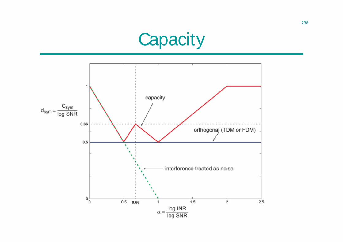
238
Capacity
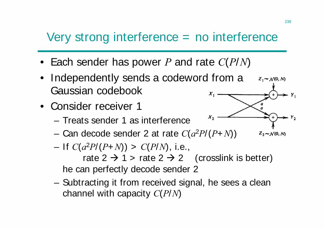
239
Very strong interference = no interference
• Each sender has power P and rate C(P/N)• Independently sends a codeword from a
Gaussian codebook• Consider receiver 1
– Treats sender 1 as interference– Can decode sender 2 at rate C(a2P/(P+N))– If C(a2P/(P+N)) > C(P/N), i.e.,
rate 2 1 > rate 2 2 (crosslink is better)he can perfectly decode sender 2
– Subtracting it from received signal, he sees a clean channel with capacity C(P/N)
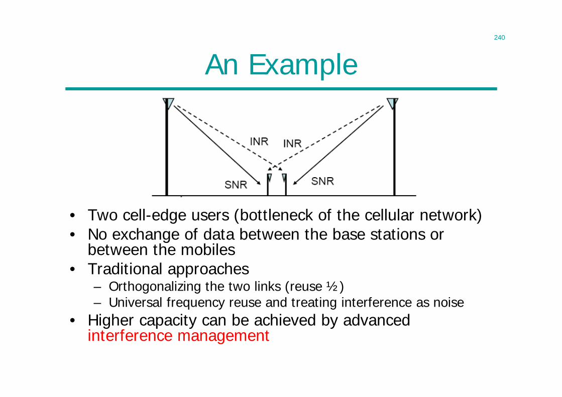
240
An Example
• Two cell-edge users (bottleneck of the cellular network)• No exchange of data between the base stations or
between the mobiles• Traditional approaches
– Orthogonalizing the two links (reuse ½)– Universal frequency reuse and treating interference as noise
• Higher capacity can be achieved by advanced interference management
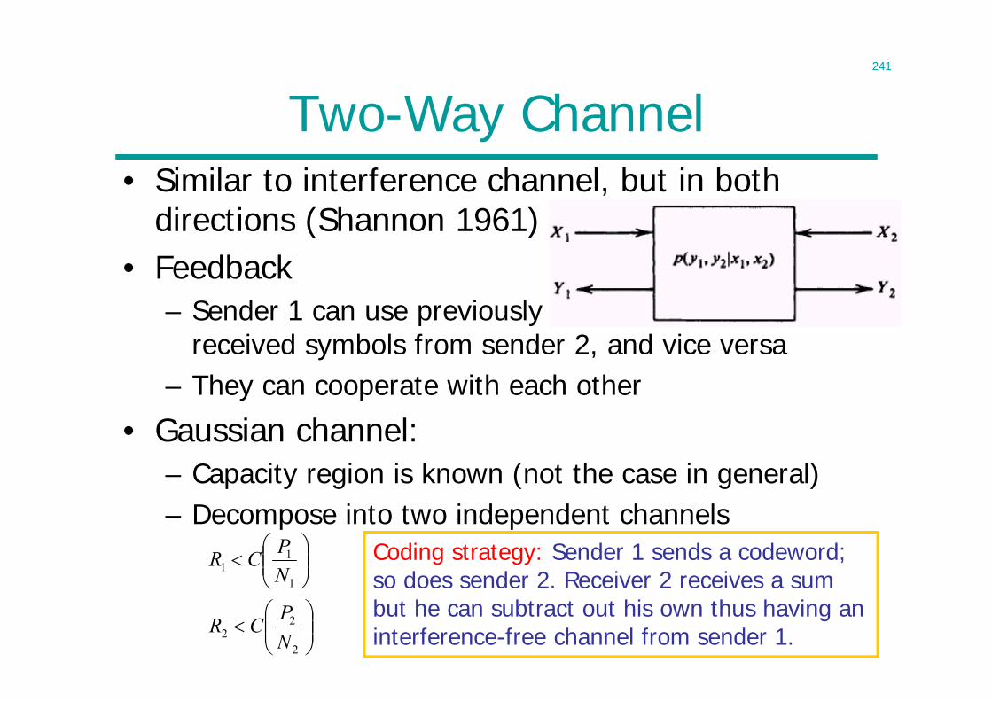
241
Two-Way Channel• Similar to interference channel, but in both
directions (Shannon 1961)• Feedback
– Sender 1 can use previouslyreceived symbols from sender 2, and vice versa
– They can cooperate with each other
• Gaussian channel:– Capacity region is known (not the case in general)– Decompose into two independent channels
2
22
1
11
NPCR
NPCR Coding strategy: Sender 1 sends a codeword;
so does sender 2. Receiver 2 receives a sum but he can subtract out his own thus having an interference-free channel from sender 1.
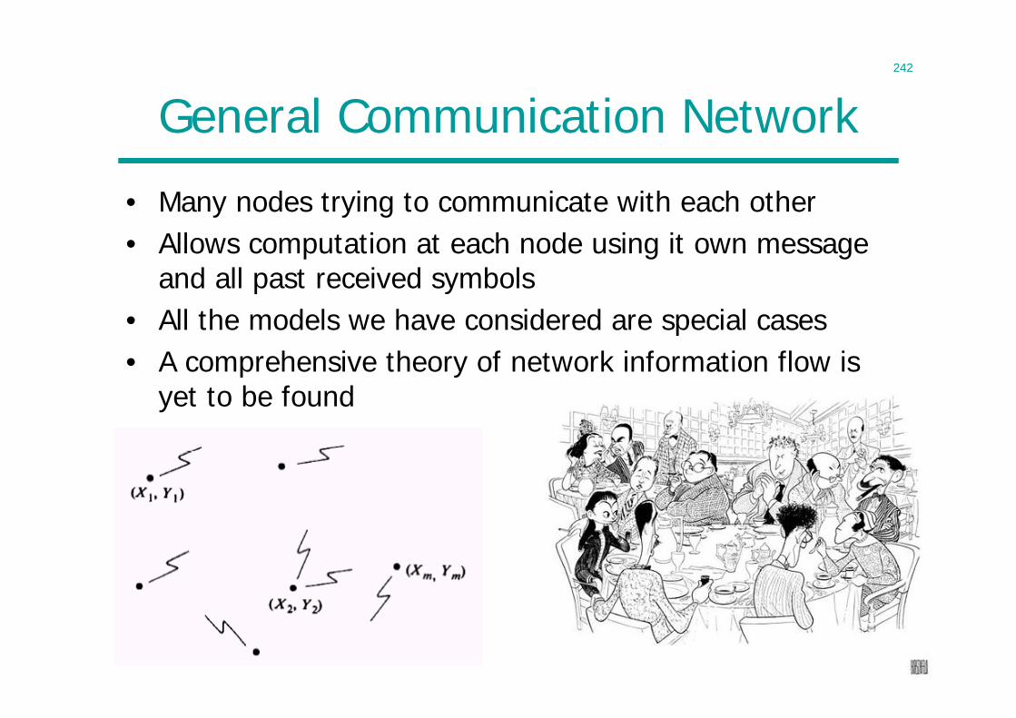
242
General Communication Network
• Many nodes trying to communicate with each other• Allows computation at each node using it own message
and all past received symbols• All the models we have considered are special cases• A comprehensive theory of network information flow is
yet to be found
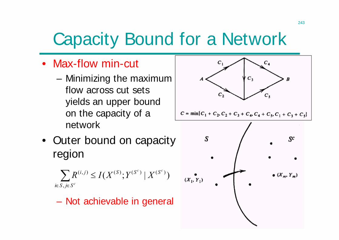
243
Capacity Bound for a Network• Max-flow min-cut
– Minimizing the maximumflow across cut sets yields an upper bound on the capacity of a network
• Outer bound on capacity region
– Not achievable in general
)|;( )()()(
,
),( cc
c
SSS
SjSi
ji XYXIR
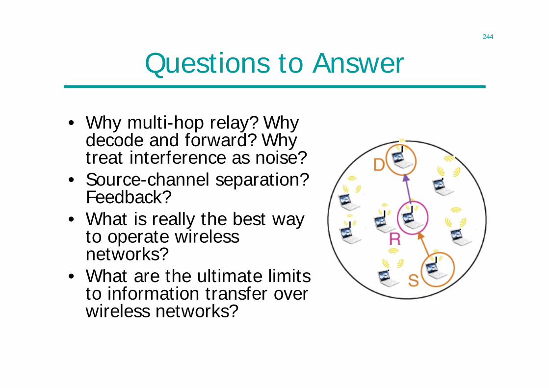
244
Questions to Answer
• Why multi-hop relay? Why decode and forward? Why treat interference as noise?
• Source-channel separation? Feedback?
• What is really the best way to operate wireless networks?
• What are the ultimate limits to information transfer over wireless networks?
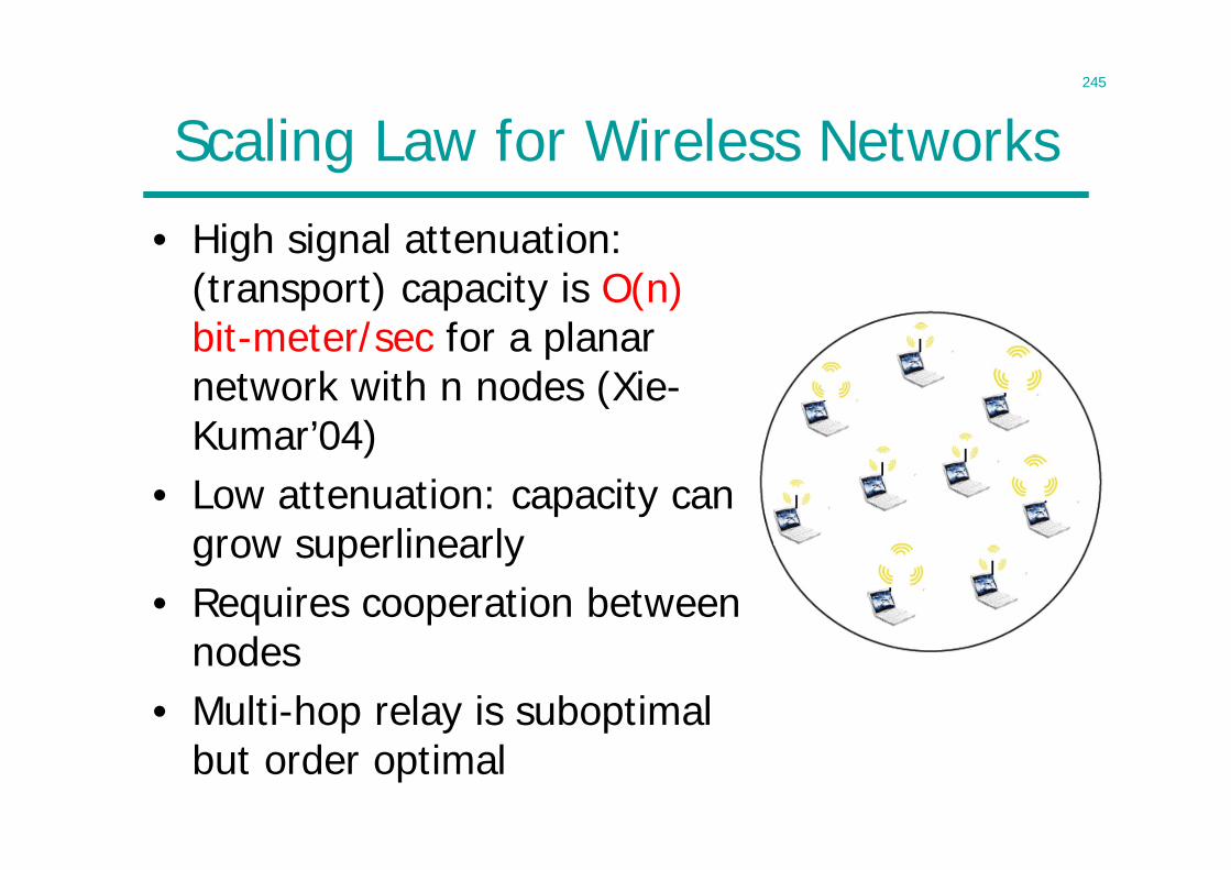
245
Scaling Law for Wireless Networks
• High signal attenuation: (transport) capacity is O(n) bit-meter/sec for a planar network with n nodes (Xie-Kumar’04)
• Low attenuation: capacity can grow superlinearly
• Requires cooperation between nodes
• Multi-hop relay is suboptimal but order optimal
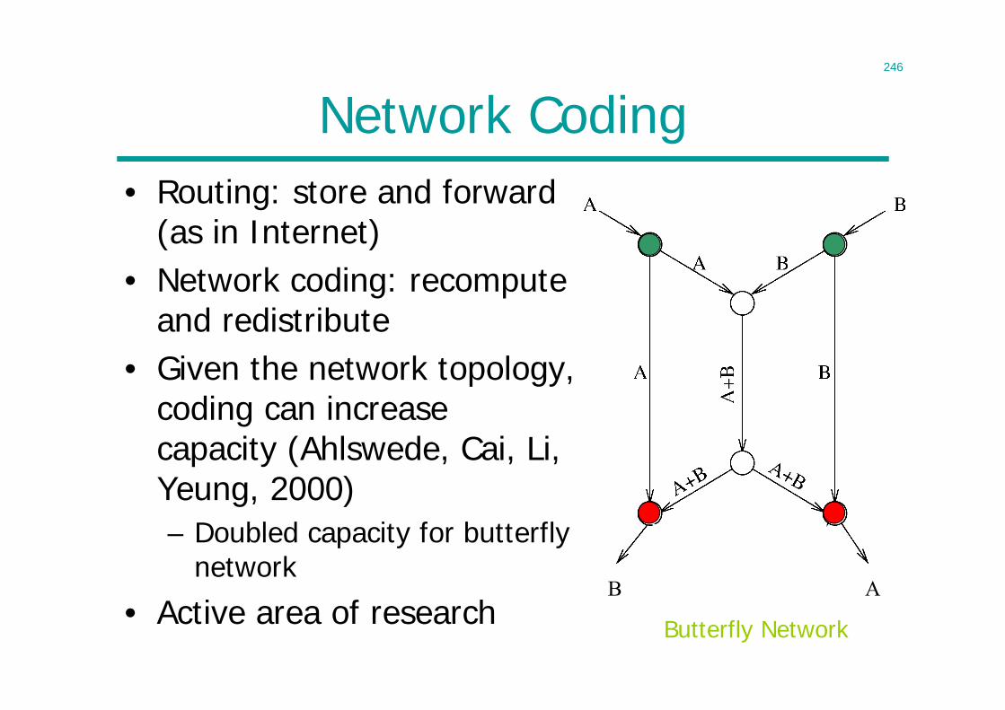
246
Network Coding• Routing: store and forward
(as in Internet)• Network coding: recompute
and redistribute• Given the network topology,
coding can increase capacity (Ahlswede, Cai, Li, Yeung, 2000)– Doubled capacity for butterfly
network
• Active area of researchB A
Butterfly Network

247
Lecture 18
• Revision Lecture
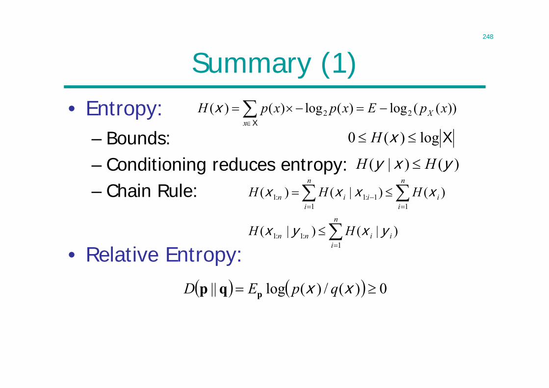
248
Summary (1)• Entropy:
– Bounds:– Conditioning reduces entropy:– Chain Rule:
• Relative Entropy:
))((log)(log)()( 22 xpExpxpH Xx
X
x
Xlog)(0 xH
)()|( yxy HH
n
iiinn
n
ii
n
iiin
HH
HHH
1:1:1
111:1:1
)|()|(
)()|()(
yxyx
xxxx
0)(/)(log|| xx qpED pqp
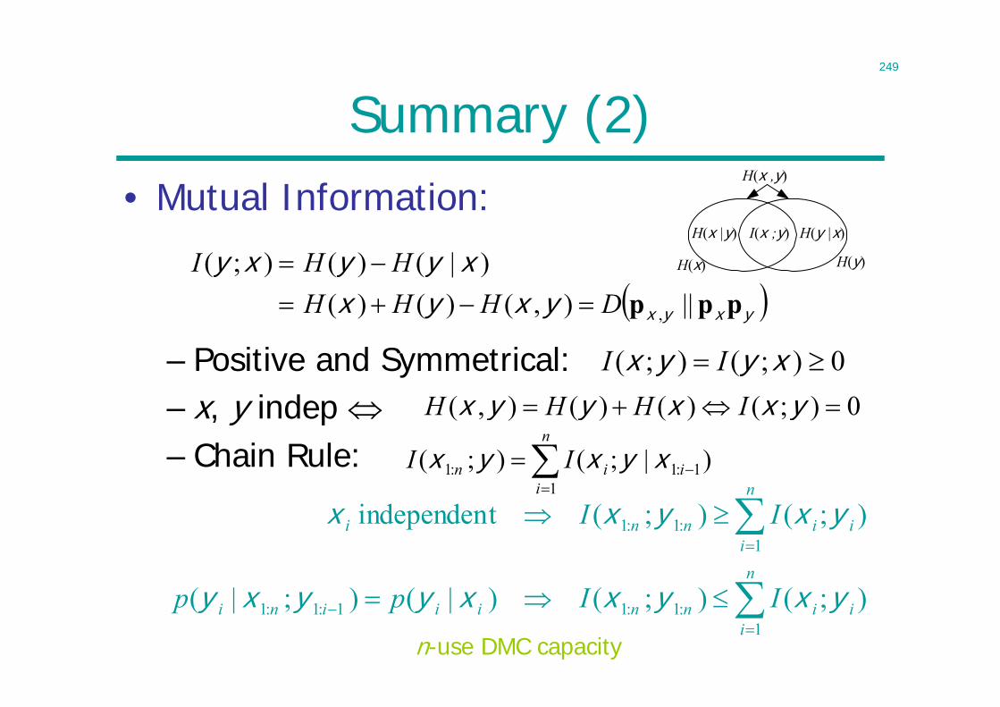
249
Summary (2)• Mutual Information:
– Positive and Symmetrical:– x, y indep – Chain Rule:
0);()()(),( yxxyyx IHHH
yxyxyxyxxyyxy
ppp ||),()()()|()();(
,DHHHHHI
0);();( xyyx II
n
iiin II
11:1:1 )|;();( xyxyx
n
iiinniiini
n
iiinni
IIpp
II
1:1:11:1:1
1:1:1
);();()|();|(
);();(tindependen
yxyxxyyxy
yxyxx
H(x |y) H(y |x)
H(x ,y)
H(x) H(y)
I(x ;y)
n-use DMC capacity
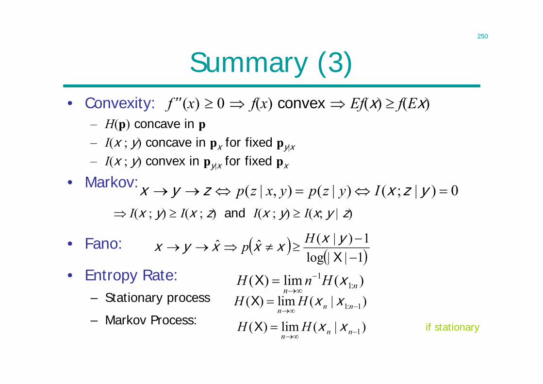
250
Summary (3)• Convexity: f’’ (x) 0 f(x) convex Ef(x) f(Ex)
– H(p) concave in p– I(x ; y) concave in px for fixed py|x
– I(x ; y) convex in py|x for fixed px
• Markov:
I(x ; y) I(x ; z) and I(x ; y) I(x; y | z)
• Fano:
• Entropy Rate:– Stationary process
– Markov Process:
0)|;()|(),|( yzxzyx Iyzpyxzp
1||log1)|(ˆˆ
Xyxxxxyx Hp
)(lim)( :11
nnHnH x
X
1: 1( ) lim ( | )n nnH H
X x x
)|(lim)( 1 nnn
HH xxX if stationary
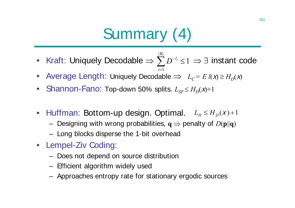
251
Summary (4)
• Kraft: Uniquely Decodable instant code
• Average Length: Uniquely Decodable LC = E l(x) HD(x)
• Shannon-Fano: Top-down 50% splits. LSF HD(x)+1
• Huffman: Bottom-up design. Optimal.– Designing with wrong probabilities, q penalty of D(p||q)– Long blocks disperse the 1-bit overhead
• Lempel-Ziv Coding:– Does not depend on source distribution– Efficient algorithm widely used– Approaches entropy rate for stationary ergodic sources
1||
1
X
i
liD
1)( xDH HL
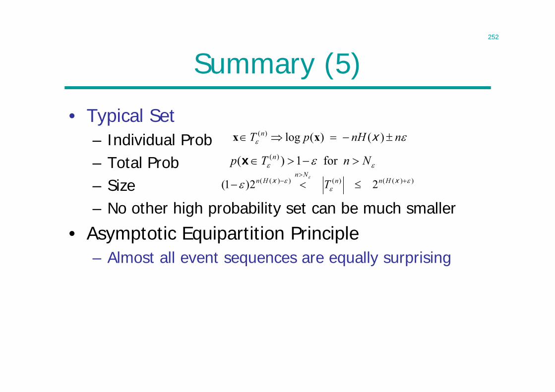
252
Summary (5)
• Typical Set– Individual Prob– Total Prob– Size– No other high probability set can be much smaller
• Asymptotic Equipartition Principle– Almost all event sequences are equally surprising
nnHpT n )()(log)( xxx
NnTp n for 1)( )(x
22)1( ))(()())((
xx HnnNn
Hn T
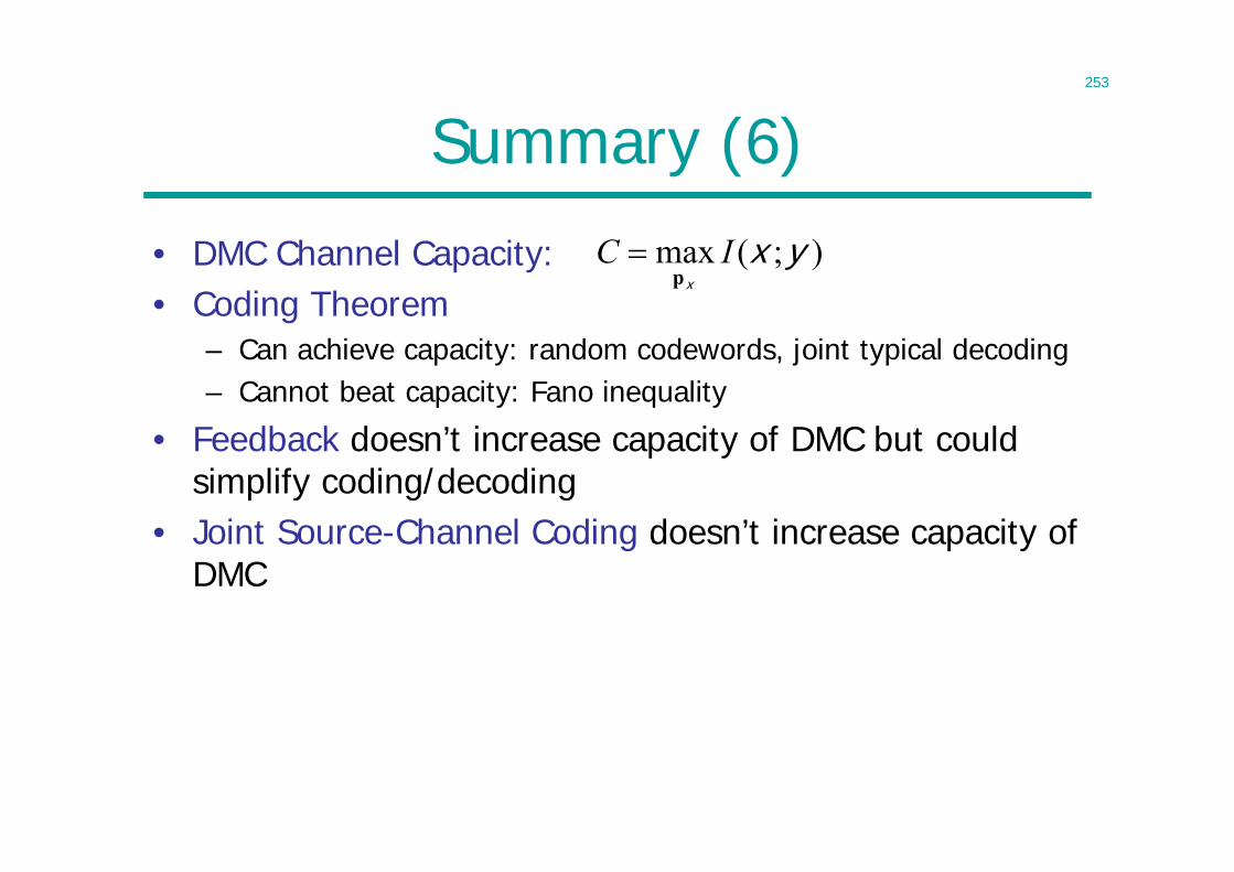
253
Summary (6)
• DMC Channel Capacity:• Coding Theorem
– Can achieve capacity: random codewords, joint typical decoding– Cannot beat capacity: Fano inequality
• Feedback doesn’t increase capacity of DMC but could simplify coding/decoding
• Joint Source-Channel Coding doesn’t increase capacity of DMC
);(max yxx
ICp
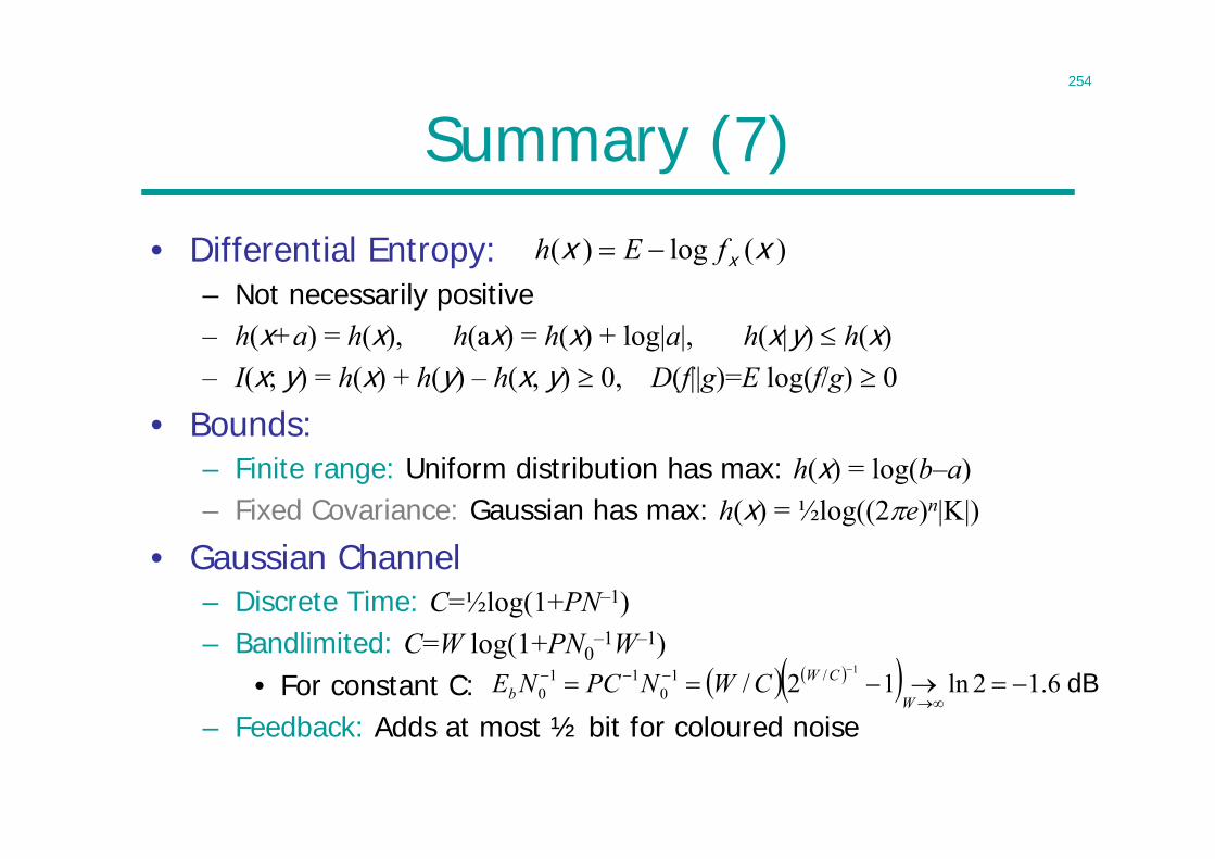
254
Summary (7)
• Differential Entropy:– Not necessarily positive– h(x+a) = h(x), h(ax) = h(x) + log|a|, h(x|y) h(x) – I(x; y) = h(x) + h(y) – h(x, y) 0, D(f||g)=E log(f/g) 0
• Bounds:– Finite range: Uniform distribution has max: h(x) = log(b–a)– Fixed Covariance: Gaussian has max: h(x) = ½log((2e)n|K|)
• Gaussian Channel– Discrete Time: C=½log(1+PN–1)– Bandlimited: C=W log(1+PN0
–1W–1)• For constant C:
– Feedback: Adds at most ½ bit for coloured noise
)(log)( xx xfEh
dB 6.12ln12/1/1
011
0
W
CWb CWNPCNE

255
Summary (8)
• Parallel Gaussian Channels: Total power constraint– White noise: Waterfilling:– Correlated noise: Waterfill on noise eigenvectors
• Rate Distortion:
– Bernoulli Source with Hamming d: R(D) = max(H(px)–H(D),0)– Gaussian Source with mean square d: R(D) = max(½log(2 D–1),0)
– Can encode at rate R: random decoder, joint typical encoder
– Can’t encode below rate R: independence bound
iP nP max ,0i iP v N
)ˆ;(min)()ˆ,(..|ˆ
xxxxxx
IDRDEdts
p
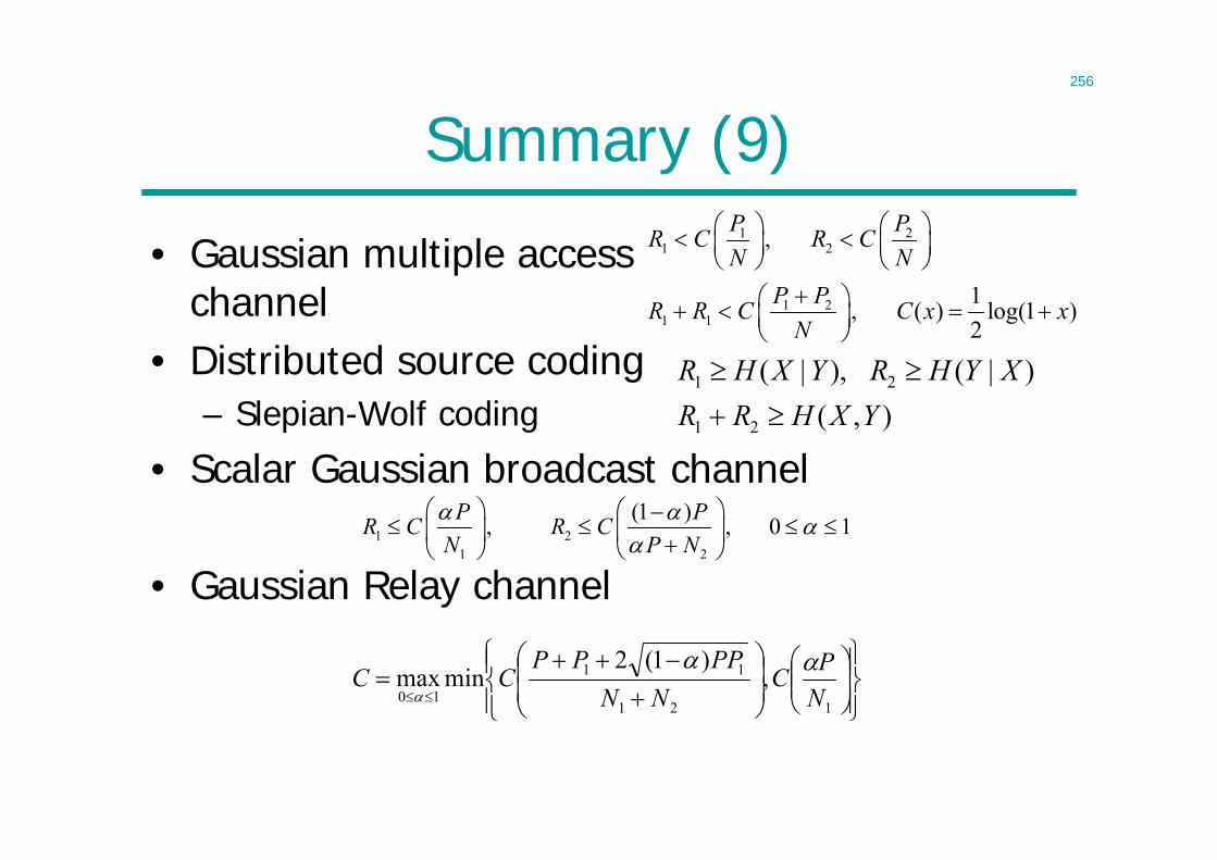
256
Summary (9)
• Gaussian multiple access channel
• Distributed source coding– Slepian-Wolf coding
• Scalar Gaussian broadcast channel
• Gaussian Relay channel
1 21 2
1 21 1
,
1, ( ) log(1 )2
P PR C R CN N
P PR R C C x xN
1 2
1 2
( | ), ( | )( , )
R H X Y R H Y XR R H X Y
1 21 2
(1 ), , 0 1P PR C R CN P N
121
11
10,
)1(2minmax
NPC
NNPPPP
CC
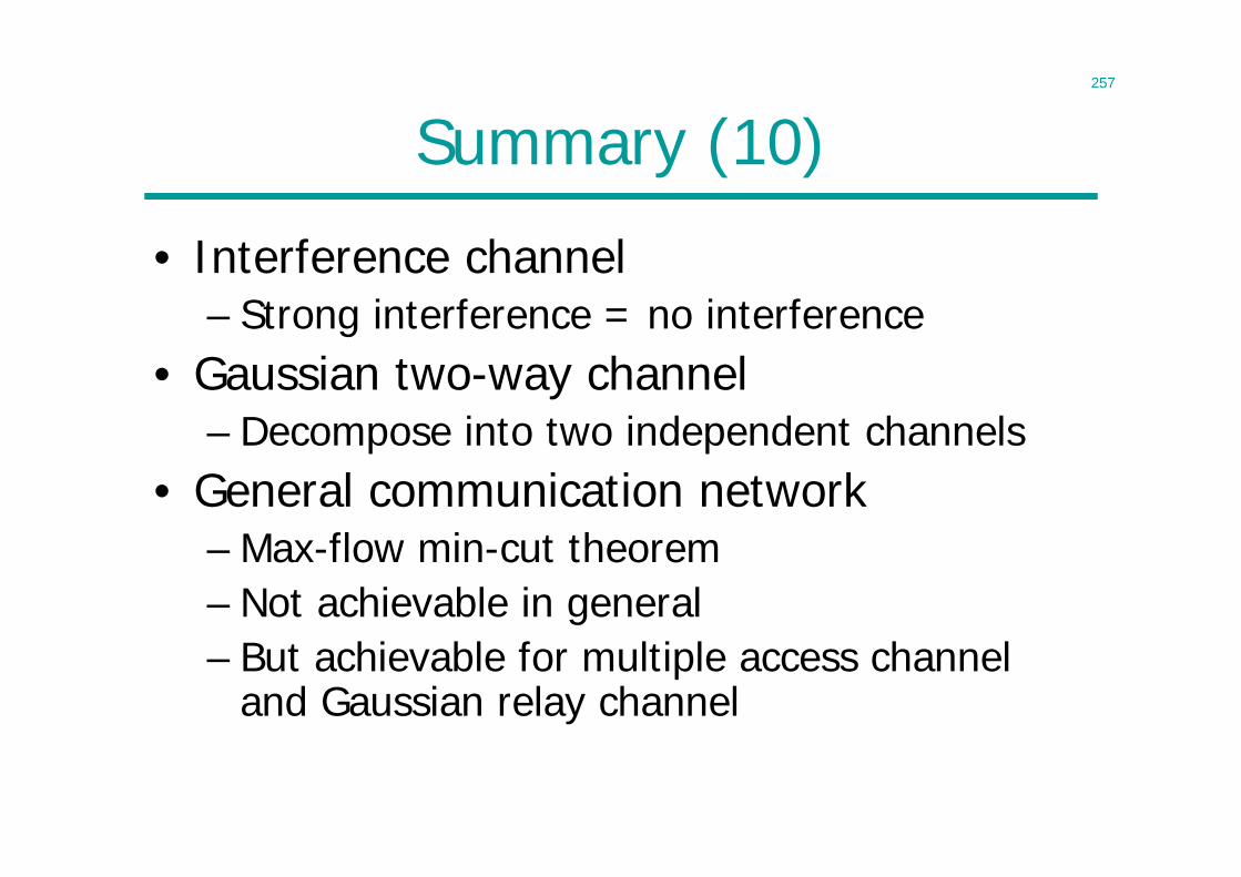
257
Summary (10)
• Interference channel– Strong interference = no interference
• Gaussian two-way channel– Decompose into two independent channels
• General communication network– Max-flow min-cut theorem– Not achievable in general– But achievable for multiple access channel
and Gaussian relay channel