information technology, organisational change and

Draft, please do not quote. Comments welcome.

Information Technology, Organisational Change and Productivity

Growth: Evidence from UK firms *

Gustavo Crespi University of Sussex and CeRiBA

Chiara Criscuolo

OECD and CeRiBA

Jonathan Haskel Queen Mary, University of London; AIM, CeRiBA, CEPR and IZA

June 2005

Keywords: Productivity Growth, ICT, Organisational change JEL classification: D24, J24

Abstract We use panel data on productivity, ICT and organisational change in UK establishments to examine the relationship between productivity growth, ICT and organisational change (∆O). Consistent with the small number of other micro studies we find that ICT and ∆O interact in their effect on productivity growth. but there is no interaction between ∆O and non-ICT investment. Some new findings are (a) ∆O is affected by competition and (b) we also find strong effects on the probability of introducing ∆O from ownership. US-owned firms, operating in the UK, are much more likely to introduce ∆O relative to other firms.

*Contact: Jonathan Haskel, Queen Mary, University of London, Economics Dept, London E1 4NS, j.e.

[email protected]. Financial support for this research comes from the ESRC/EPSRC Advanced Institute of Management Research, grant number RES-331-25-0030. This work was carried out at The Centre for Research into Business Activity, CeRiBA, at the Business Data Linking Branch at the ONS. This work contains statistical data from ONS which is crown copyright and reproduced with the permission of the controller HMSO and Queen's Printer for Scotland. The use of the ONS statistical data in this work does not imply the endorsement of the ONS in relation to the interpretation or analysis of the statistical data. We thank Ray Lambert for all his help with the CIS and the BDL team at ONS as usual for all their help with computing and facilitating reseach. All errors are of course our own.

1

mailto:[email protected]

1 Introduction

The impact of ICT on productivity growth is a key area of research. The early literature was

faced with the Solow puzzle, namely that computers seemed to be everywhere but in the

productivity statistics. Growth accountants offered an explanation: since computers in the early

1990s were only a relatively small fraction of overall capital stock their impact on productivity

growth was limited. Recently a second, related puzzle, has emerged: why does it seem to take

time for computer investment to show up in productivity growth? This is of specific interest to

Europeans since in many European countries the share of computers in capital is similar to the

US but (total factor) productivity acceleration has been either zero or even negative.

One suggested answer to this second puzzle is that computer investment requires

complementary investment in organisational change (∆O) to obtain productivity gains.1 Thus if

some firms or nations do not undertake such investment, they fail to get the productivity gains,

or, whilst they are undertaking such investment their measured productivity might slow since

they are devoting resources to such investment which are not measured as such.

Such an answer is consistent (to some extent) with the macro data (Basu et al, 2003), but

without a ready macro measure of organisational change it is still rather a matter of conjecture.

One possibility is to turn to micro data. However, there is very little micro evidence, for two

main reasons. First, it is very hard to find micro data on output, ICT and other inputs and

organisational measures. Three well-cited papers are Bresnahan, Brynjolfsson and Hitt (2002),

papers by Ichniowski and Shaw and co-authors (summarised in Ichniowski and Shaw,2003) and

Black and Lynch (2003) but this literature is still small. Second, as is well acknowledged in

these studies, organisational change is likely endogenous and so such an explanation would be

more convincing if there were an explanation of what drives organisational change in firms.

This current paper uses panel data on productivity, ICT and organisational change in UK

establishments to try to shed light on both these questions. Some of our findings we believe to

be of interest since they are consistent with findings in data for other countries. But some of our

findings we believe add to the extant literature.

1 A alternative is the poor EU productivity growth results in large part from relatively poor productivity growth in

wholesaling and retailing. This might in turn be due in part to planning regulations, but since wholesaling and retailing uses ICT intensively it could also be due to relatively “poor” use of the ICT capital stock.

2

We have three findings that are consistent with other studies. First, ICT appears to have

high returns in a growth accounting sense when one omits ∆O. When ∆O is included the ICT

returns are greatly reduced. Second, ICT and ∆O interact in their effect on productivity growth.

Third, there is no impact on productivity growth from ∆O and non-ICT investment. These

findings are all then consistent with the suggestion from the macro data and the evidence from

the micro data that ICT and ∆O together boost productivity growth (Brynjolfsson and Hitt; 2001,

Bresnahan, Brynjolfsson and Hitt, 2002).

We have in addition, two broad findings that, we believe, add to the extant literature.

First, we find that ∆O is affected by competition. When we measure competition by lagged

changes in market share we find that firms who lose market share in previous periods are

statistically significantly more likely to introduce ∆O in the current period. Second, we also find

strong effects on the probability of introducing ∆O from ownership. US-owned firms are much

more likely to introduce ∆O relative to non-UK firms. Since our data are all for firms operating

in the UK then such firms are operating in the same environment with the same local skills base,

regulatory structure, infrastructure etc. Thus this finding is consistent with management

differences being important in explaining ∆O.

As in all empirical studies our findings should be treated with caution due, among other

things as we discuss below, measurement problems and our short panel. But our findings are

suggestive of a story that might account for the second of the ICT/productivity growth puzzles

set out above. It is that (a) successful productivity growth needs both ICT and organisational

change; (b) competition forces firms to introduce organisational change and (c) US firms,

controlling for competition, implement organisational change particularly rapidly. Quite why

they do is a matter for speculation at this point since it is not something that we can answer with

our data. Nonetheless we regard the finding of interest and suggestive of areas for future fruitful

work.

The rest of the paper proceeds as follows. In section 2 we set out a framework to

understand the key questions involved and our and other approaches. Section 3 describes the

data available and section 4 our results on the production and section 5 results for organisational

change. Section 6 summarises and concludes.

3

2 Overall approach

2.1 Simplified model

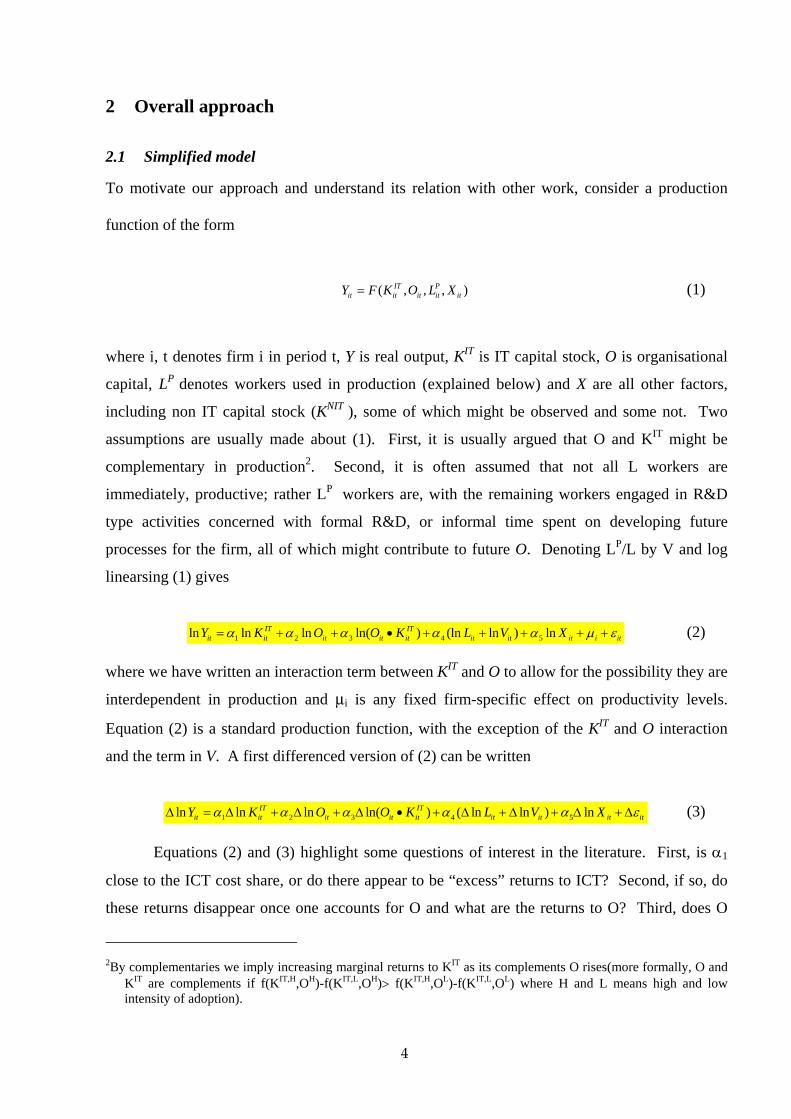
To motivate our approach and understand its relation with other work, consider a production

function of the form

(1) ( , , ,IT Pit it it it itY F K O L X= )

where i, t denotes firm i in period t, Y is real output, KIT is IT capital stock, O is organisational

capital, LP denotes workers used in production (explained below) and X are all other factors,

including non IT capital stock (KNIT ), some of which might be observed and some not. Two

assumptions are usually made about (1). First, it is usually argued that O and KIT might be

complementary in production2. Second, it is often assumed that not all L workers are

immediately, productive; rather LP workers are, with the remaining workers engaged in R&D

type activities concerned with formal R&D, or informal time spent on developing future

processes for the firm, all of which might contribute to future O. Denoting LP/L by V and log

linearsing (1) gives

1 2 3 4 5ln ln ln ln( ) (ln ln ) lnIT ITit it it it it it it it i itY K O O K L V Xα α α α α µ ε= + + • + + + + + (2)

where we have written an interaction term between KIT and O to allow for the possibility they are

interdependent in production and mi is any fixed firm-specific effect on productivity levels.

Equation (2) is a standard production function, with the exception of the KIT and O interaction

and the term in V. A first differenced version of (2) can be written

1 2 3 4 5ln ln ln ln( ) ( ln ln ) lnIT ITit it it it it it it it itY K O O K L V Xα α α α α ε∆ = ∆ + ∆ + ∆ • + ∆ + ∆ + ∆ + ∆

(3)

Equations (2) and (3) highlight some questions of interest in the literature. First, is α1

close to the ICT cost share, or do there appear to be “excess” returns to ICT? Second, if so, do

these returns disappear once one accounts for O and what are the returns to O? Third, does O

2By complementaries we imply increasing marginal returns to KIT as its complements O rises(more formally, O and

KIT are complements if f(KIT,H,OH)-f(KIT,L,OH)> f(KIT,H,OL)-f(KIT,L,OL) where H and L means high and low intensity of adoption).

4

and KIT interact in (2) or (3)? Fourth, if implementing ICT requires labour resources to be

directed away from production so that V falls in periods of ICT investment does failure to

measure V lead to measured TFP growth falling in such periods? Fifth, what determines O (and

indeed the other variables)?

The equations also highlight some of the problems in answering these questions. First,

data on all these variables is rarely found. Many company level data sets might have data on Y

and K but few also have data on ICT and fewer still also data on O. Second, if O is endogenous

and correlated with omitted variables in (2) or (3) then α2 and α3 are biased. For example, if

managerial quality is not measured and is not in X and if better managers raise Y and also

implement O (better organisational practices) then α2 would be upward biased in (2)3. Thus it is

hard to establish the contribution from O. Third, if we are to understand cross-country

differences in O then we need something like (2) and (3) for different countries or (2) and (3) for

one country along with data on the extent of K and O in different countries.

2.2 Existing evidence

What then is the approach of the literature to these questions? Brynjolfsson and Hitt (2003),

assemble company level data on 527 US firms, over an 8 year period, 1987-94 (with some firms

in the sample all the time and some not) with data on outputs, inputs and computers to estimate

equations like (3), which they do using a mix of long and short differences. They have no

measures of O or V however. They find long run returns to ∆Kit to exceed short run returns

which they interpret as consistent with congruent changes in O.

Bresnahan, Brynjolfsson and Hitt (2002) add data on O to these data, by using a cross-

section survey of managers in 1995 and 1996 (i.e. at the end of the other data), leaving around

300 large US firms in the sample. They measure O as a linear combination of questions on

teamworking, and the extent to which workers have authority over their pace and methods of

work. Since O is a cross section, their main results are estimates of (2), where again they have

no measures of V.4 They find statistically significant positive effects on Yit from KITit, Oit and

(Oit • KITit) and emphasise the interaction between O and KIT

it.

Black and Lynch (2001a) obtain two cross-sections of data on O for 1993 and 1996, in

their case indications of the use of high performance work systems, and combine this with a

3 Note that by taking first difference in (3) we are removing those firm level unobserved factors that remain fixed

over time. 4 They do argue that since the work practices in O are likely to be new, they might be measures of ∆O.

5

panel of firm data. Estimating both cross sections like (2) and panels like (3), they find that high

performance workplace practices are associated with higher productivity and in particular that

non-managers using computers is positively correlated with productivity.

There are of course a number of studies that look at highly related issues but not using IT.

For example, Black and Lynch (2001b) obtain a cross-section of data on O for 1994, in their case

indications of the use of high performance work systems, and combine this with a panel of firm

data for 1987-93. They estimate (2) and find significant effects from O on Y/L. However they

have in that study no data on KIT.5

A rather smaller literature is concerned with the determinants of O or ∆O. Nickell,

Nicolitsas and Patterson (2001) focus on the determinants of ∆Oit, using data on 66 UK

manufacturing firms 1981-86 using as their measure firms who report whether they (a) removed

restrictive practices or not and (b) introduced new technology. They also use 98 firms who were

surveyed in 1993/4 as regards changes in their management practices. They find that financial

and market pressure, the latter measured by lagged changes in market share, are more likely to

make firms introduce innovations in O.

Finally, Boning, Ichniowski and Shaw (2001) study both the productivity impact of O

and the determinants of O using data on physical output of US minimills for productivity and

teamworking for O. In their study, teamworking boosts productivity and the decision to adopt

teamworking is driven by things like plant characteristics (i.e. whether the plant is old or not),

the complexity of the good produced and older and longer tenured managers. Their focus is not

so much on IT however.

There are of course a number of unresolved issues with these studies. First, there are

relatively few and hence more studies would be of interest. Second, not all the studies deal

explicitly with IT. Third, it would be desirable to have some studies for services given that this

is where much of the IT capital stock is invested. Fourth, whilst it seems plausible that O or ∆O

are affected by technological factors it also seems plausible that they are affected by competition.

Fifth, it would be helpful to understand why different countries seem to perform so differently.

Thus our strategy is to try to estimate (3) with data on IT and O and an equation for ∆O namely

5 There is of course a related literature that has no data on IT or on O but looks at a number of proxies that might

determine O, most notably unions, product market competition or ownership. On unions for example Clark (1994) and Haskel (2005) find a negative effect on US and UK data, whilst Freeman and Medoff (1978) find a positive effect on productivity all of which is consistent with unions affecting O. On competition, Nickell (1996) finds a positive effect of increased competitive pressure on TFP growth, consistent with competition affecting O.

6

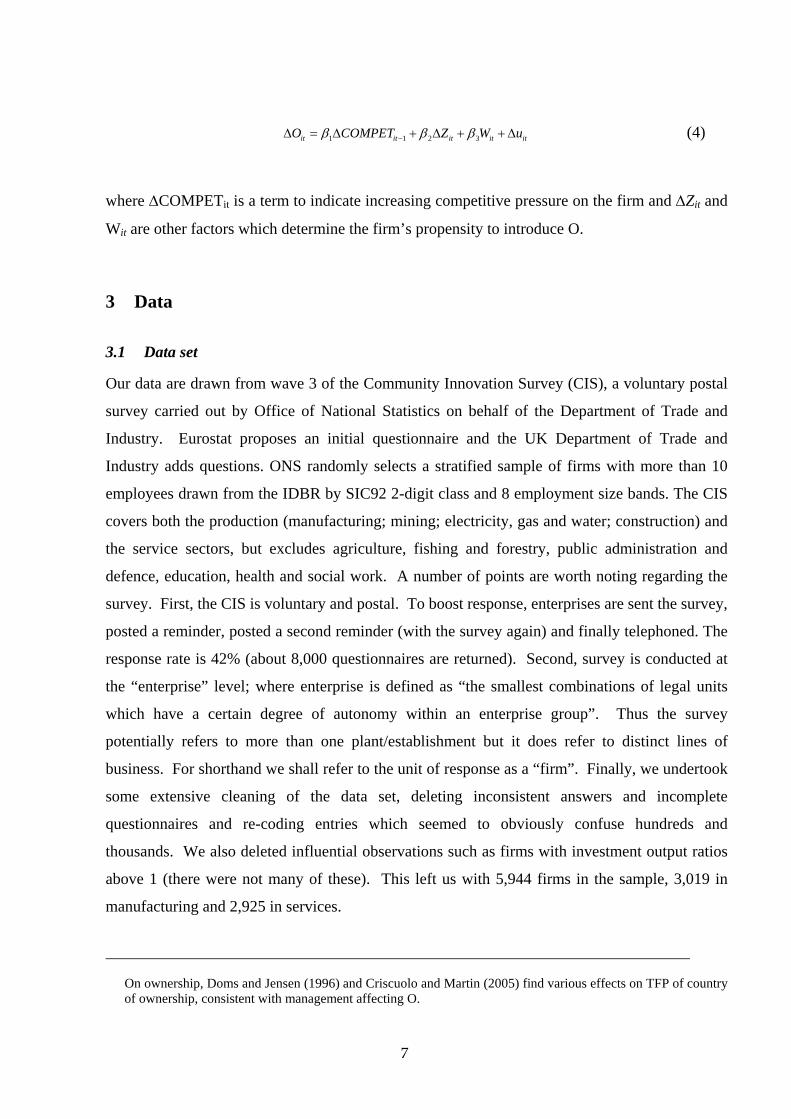
1 1 2 3it it it it itO COMPET Z W uβ β β−∆ = ∆ + ∆ + + ∆ (4)

where ∆COMPETit is a term to indicate increasing competitive pressure on the firm and ∆Zit and

Wit are other factors which determine the firm’s propensity to introduce O.

3 Data

3.1 Data set

Our data are drawn from wave 3 of the Community Innovation Survey (CIS), a voluntary postal

survey carried out by Office of National Statistics on behalf of the Department of Trade and

Industry. Eurostat proposes an initial questionnaire and the UK Department of Trade and

Industry adds questions. ONS randomly selects a stratified sample of firms with more than 10

employees drawn from the IDBR by SIC92 2-digit class and 8 employment size bands. The CIS

covers both the production (manufacturing; mining; electricity, gas and water; construction) and

the service sectors, but excludes agriculture, fishing and forestry, public administration and

defence, education, health and social work. A number of points are worth noting regarding the

survey. First, the CIS is voluntary and postal. To boost response, enterprises are sent the survey,

posted a reminder, posted a second reminder (with the survey again) and finally telephoned. The

response rate is 42% (about 8,000 questionnaires are returned). Second, survey is conducted at

the “enterprise” level; where enterprise is defined as “the smallest combinations of legal units

which have a certain degree of autonomy within an enterprise group”. Thus the survey

potentially refers to more than one plant/establishment but it does refer to distinct lines of

business. For shorthand we shall refer to the unit of response as a “firm”. Finally, we undertook

some extensive cleaning of the data set, deleting inconsistent answers and incomplete

questionnaires and re-coding entries which seemed to obviously confuse hundreds and

thousands. We also deleted influential observations such as firms with investment output ratios

above 1 (there were not many of these). This left us with 5,944 firms in the sample, 3,019 in

manufacturing and 2,925 in services.

On ownership, Doms and Jensen (1996) and Criscuolo and Martin (2005) find various effects on TFP of country of ownership, consistent with management affecting O.

7

3.2 Data on ∆O

We use the CIS to try to measure ∆O, changes in organisational capital at the firm. The

distinction used by Ichniowski and Shaw (1993, p.158) is between a “scientific technology

shock” and an “organisational technology shock”. From the production function we might

interpret this as a distinction between embodied and disembodied changes, whereby any

technology changes embodied in capital should not be thought of as part of ∆O. Bresnahan et al

(2002) for example use data on teamworking as their measure of disembodied organisational

capital i.e. something that does not necessarily involve different capital; fast turn around of

airliners by low-cost airlines might be another (as opposed to a computerised booking system to

make reservations over the web which we might think of as an embodied technology). The

organisational/scientific distinction seems to be a distinction suited to our data. The CIS opening

questionnaire paragraph says

We begin by looking at innovation based on the results of new technological developments, new combinations of existing technology or utilisation of other knowledge held or acquired by your enterprise….The final part of the questionnaire broadens the focus to consider organisational and management changes.

Since the questionnaire refers to changes, we shall try to use its answers to build measures of

∆O. 6 Let us start with the final part of the questionnaire relating to “…organisational and

management changes” which seems to be the closest in sprit to the disembodied nature of ∆O.

The question is

17. Wider innovation 17.1 Did your enterprise make major changes in the following areas of business structure and

practices during the period 1998-2000 and how far did business performance improve as a result?

a. Implementation of new or significantly changed corporate strategies e.g. mission statement, market share.

b. Implementation of advanced management techniques within your firm e.g. knowledge management, quality circles.

6 It is worth highlighting to how difficult it is to measure O. Whilst e.g. teamworking might be part of O there might

be very many other aspects of a firm’s O: morale, consultation methods, lean production, family-friendly work practices etc. and thus any questionnaire is almost bound to provide only a partial measure, as Bresnahan acknowledge. This suggests that it might be easier to try to measure DO, as we try to here, as opposed to the level of O. In addition whilst our questions on DO are rather broad, making the precise elasticity of a particular dimension of O hard to estimate, the broadness might help if O is in reality a range of aspects at the firm. Note that Bresnahan et al argue that their (composite) work organisation measure at a particular period might be a measure of DO if the work practices they measure have been newly introduced.

8

c. Implementation of new or significantly changed organisational structures e.g. Investors in People, diversification.

d. Changing significantly your firms marketing concepts/ strategies e.g. marketing methods.

Firms are given the options to answer “not used” and impact on performance “low”, “medium”

and “high”. We ignore the impact part of the answer since it might not meaningfully vary

between firms and be endogenous in a productivity study and therefore we reduce each answer to

a 1/0 yes/no. Answers to (b) and (c) would appear to proxy changes in organisational capital at

firms. Answers to (a) and (d) are more difficult to interpret since they may or may not have

involved changes in organisational capital. On the other hand, firms are asked (a) first which

might affect their propensity to answer the other questions. For the moment, we combined them

but we shall inspect the robustness of this below.

Table 1, column 1 sets out data on these wider innovations. 65% and 62% of firms

(unweighted) report implementing ∆O. The rest of the table shows the other innovations which

we shall come to.

As the above quote suggests, firms are in addition asked about their more technological

innovations. They are asked about what are called “process” and “product” innovations. We

deal with product innovations below, here we discuss whether process innovation should be part

of ∆O or some other part of the production function. The question is follows:

5.Process Innovation. “For this survey process innovation is the use of new or significantly improved technology for

production or the supply of goods and services. Purely organisational or managerial changes should not be included. For examples of process innovations see front cover”

During the three year period 1998-2000, did your enterprise introduce any new or

significantly improved processes for producing or supplying products (goods or services) which were new to your firm?

The examples of process innovations on the front of the questionnaire are as follows:

EXAMPLES OF PROCESS INNOVATIONS Linking of Computer Aided Design station to parts suppliers Introduction of Electronic Point of Sale equipment in Garden Centre Digitising of pre-press in printing house Robotised welding EXAMPLES WHICH ARE NOT TECHNOLOGICAL INNOVATION The renaming and repackaging of an existing soft drink popular with older people, to establish

a link with a football team in order to reach the youth market, is not a technology based innovation as defined in this survey, but could register as a marketing change in question 17. New models of complex products, such as cars or television sets, are not product

9

innovation, if the changes are minor compared with the previous models, for example offering a radio in a car.

The examples of process innovations on the front cover seem to be examples of embodied

changes, in particular changes in ICT. If they are captured in ∆KIT and ∆KNIT then this suggests

they might not be included in ∆O. Indeed, the description just before the actual question seems

to re-inforce this view. However, to investigate this further however we proceeded as follows.

Firms are asked

5.4 Please give a short description of your most important process innovation:

Around 1200 firms responded to having done any sort of process innovation but only 874

provide some description of it. To analyse what they say we searched each sentence for any

word we thought to be related to the hardware part of information technologies (IT) investment

(key words used are: computer/s, automation, automatic digitalisation, cnc, digital, automated,

robotic, cad, networking, digitising, pc, computerisation, it, cam, network, robot, hardware,

satellite, robotisation and automating. These keywords were generated after the analysis of a

random sample of about 100 reported process innovations. We then generated a new dummy

variable called HARDWARE if any of these words was present.

We then applied the same procedure in order to detect the software component of

information technologies, using the keywords: website, email, online, on-line, internet, web,

software, virtual, programming, e-commerce, edi, cctv, programmes, application, intranet and

email and generating a new dummy variable called SOFTWARE.7. Finally, we applied the

procedure to identify lean process innovations, with keywords outsourced, coding, bar, lean,

cell, sourcing, management, planning, outsourcing, layingout, iso, just, layout, cellular, logistics,

kanbam, kanbams, stock and re-organise and a new dummy variable called LEAN if any of

these words was present in any of the new variables-words. Finally, for those cases with no

match match with any of the above mentioned key words, we created a category called “NON-

IDENTIFIED”. This category includes typical very complex descriptions that might suggest a

more advanced sort of process innovations (for example: installation of steel wire armouring

machinery, improved petal and leaf cutting, precision cooking and slicing equipment

7 In this case some text cleaning was required because there were several cases with the phrase “computer software”,

which was cleaned to just “software”.

10

introduction of spectrophotometer for more accurate shade matching). Many of these words

seems to imply the introduction of some sort of “machinery”.

Because there was some degree of overlapping among the different classes, some results

were re-allocated in order to have classes that are fully exclusive. If there was an overlap

between HARDWARE and SOFTWARE the observation was allocated only to SOFTWARE,

because it is the class with fewer cases. Following in the same way, if there is an overlap

between SOFTWARE and LEAN the observation was allocated only to the last one, and so on.

Hence, in the results of below the categories will be fully exclusive. Table 2 shows the results of

this analysis. The largest category is still the non-identified case with 53% of the cases. Looking

at the other categories, about 22% are hardware related process innovations, 15% are software

related process innovations and less than 9% correspond to lean process innovations. Thus it

would seem reasonable to assume that whilst many reported process innovations are machinery

related, especially to IT, at least some of the reported process innovations are possibly

disembodied since they refer to new sorts of production.

To further investigate this question further we split up firms into all the possible

combinations of ICT, organisational change and process innovation. Thus this does not confine

us to just those firms who answered yes to process innovation and then filled out the most

significant innovation. The results are set out in Table 3 from which a number of points are

worth making. First, the largest group is those who did only organisational change with no

process or IT investment (33.7% of firms), consistent with the ideas that reported organisational

is potentially disembodied from ICT capital. Second, 6.71% of firms report doing process

innovation but no spending on IT (1.43 with no organisational change, 5.28 with) suggesting

that, as above, part of process innovation might not necessarily be embodied in IT capital. Third,

can we enter organisational change and process innovation as separate measures of ∆O? Since

we will enter ICT as well identification of these measures separately would rely on sufficient

firms undertaking them in isolation.8 The problem is that, as Table 3 shows, only 1.43% of firms

undertook only process innovation with no organisational change or ICT. Thus we are not

confident that we can enter organisational change and process innovation as separate measures of

∆O and identify them reliably (this indeed turned out to be the case, both terms and their

interactions were ill determined). Therefore we combined them together as part of ∆O.

8 This is not strictly correct since we use ICT as a continuous variable as set out below. But it gives the essential

intuition behind why in practice we cannot identify all these effects separately.

11

However, we did also re-run the regressions with just the “wider innovation” measures for ∆O,

see below.

Second, we tried to split up ∆O into process innovation and wider innovation. Our

results here were poorly determined suggesting collinearity which turned out indeed to be the

case, see below. Finally, we did experiment with novel process innovation.

Returning to Table 1, column 3 sets out data on reported process innovations. In

constrast to organisational innovations in column 2, many fewer firms report this: 25% and 16%

in manufacturing and services respectively. As column 4 shows, a variable coded 1 if firms

report either one of these and 0 otherwise is rather more even throughout. Note that the fact that

69% of firms do both shows that almost all the firms who did process innovation also did

organisational change.

3.3 Data on IT and other inputs

To estimate the rest (3) we require data on IT and other inputs. First, the CIS asks firms to report

turnover and employment (full time equivalents) 1998 and 2000. Thus we can use these data to

measure labour productivity.

Second, the CIS also asks firms to report investment in 1998 and in 2000. It also asks

firms to report on “Acquisition of machinery and equipment (including computer hardware) in

connection with product or process innovation.” Unfortunately it only asks this question for

2000. However we use it construct ICT and non-ICT investment by splitting reported

investment in 2000 into IT and Non-IT (this last one computed as a residual). Then we use the

plant level proportion of IT investment in total investment to impute the IT investment of each

plant in 1998. Finally, we interpolate IT investment and Non-IT investment between 1998 and

2000 to fill the gap in 1999, accumulate both investment over the three years and express it as a

ratio of initial turnover to have firm level investment rates.

Table 1, column 5 sets out data the fraction of firms who report any IT investment, which is 36%

and 26% in manufacturing and services respectively (20% of firms report no investment at all.

Of those who do invest, the fraction of investment accounted for is 20%. Note that the aggregate

figure for the year 2000 in the UK is 25%9).

9 For further details see Vaze (2003)

12

Finally, firms are also asked about their product innovations, which we shall use below

but not for ∆O. Firms are asked how much of their turnover is accounted for by product

innovation. Table 1, column 5 shows the average fractions, which are around 7% of turnover.

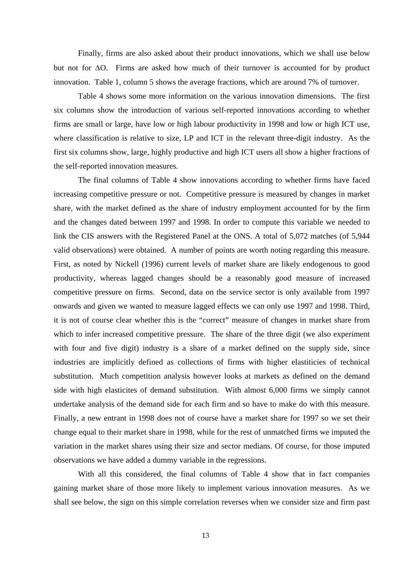
Table 4 shows some more information on the various innovation dimensions. The first

six columns show the introduction of various self-reported innovations according to whether

firms are small or large, have low or high labour productivity in 1998 and low or high ICT use,

where classification is relative to size, LP and ICT in the relevant three-digit industry. As the

first six columns show, large, highly productive and high ICT users all show a higher fractions of

the self-reported innovation measures.

The final columns of Table 4 show innovations according to whether firms have faced

increasing competitive pressure or not. Competitive pressure is measured by changes in market

share, with the market defined as the share of industry employment accounted for by the firm

and the changes dated between 1997 and 1998. In order to compute this variable we needed to

link the CIS answers with the Registered Panel at the ONS. A total of 5,072 matches (of 5,944

valid observations) were obtained. A number of points are worth noting regarding this measure.

First, as noted by Nickell (1996) current levels of market share are likely endogenous to good

productivity, whereas lagged changes should be a reasonably good measure of increased

competitive pressure on firms. Second, data on the service sector is only available from 1997

onwards and given we wanted to measure lagged effects we can only use 1997 and 1998. Third,

it is not of course clear whether this is the “correct” measure of changes in market share from

which to infer increased competitive pressure. The share of the three digit (we also experiment

with four and five digit) industry is a share of a market defined on the supply side, since

industries are implicitly defined as collections of firms with higher elastiticies of technical

substitution. Much competition analysis however looks at markets as defined on the demand

side with high elasticites of demand substitution. With almost 6,000 firms we simply cannot

undertake analysis of the demand side for each firm and so have to make do with this measure.

Finally, a new entrant in 1998 does not of course have a market share for 1997 so we set their

change equal to their market share in 1998, while for the rest of unmatched firms we imputed the

variation in the market shares using their size and sector medians. Of course, for those imputed

observations we have added a dummy variable in the regressions.

With all this considered, the final columns of Table 4 show that in fact companies

gaining market share of those more likely to implement various innovation measures. As we

shall see below, the sign on this simple correlation reverses when we consider size and firm past

13

growth, where past growth refers to employment growth computed from the Register Panel and

for the period 1997-1998.

4 Econometric implementation and results of production function

4.1 Econometric implementation

Looking at (1), let us add KNIT, non- IT capital stock and Mit, materials. If we also acknowledge

the fact that we do not have firm-specific price deflators , Pi, but industry-specific deflators, PI,

so that our measured real output is (PiYi/PI) when we can write (3) as

11 12 2 3 4

5 6 7

ln( / ) ln ln ln ln( ) ( ln ln )(ln ln ) ln ln

NIT IT ITit it It it it it it it it it

it It it it it

P Y P K K O O K L VP P M X

α α α α αα α α

∆ = ∆ + ∆ + ∆ + ∆ • + ∆ + ∆′ ε

++ ∆ − + ∆ + ∆ + ∆

(5)

Moving term by term, recall that above we mentioned that we do not have data on ∆lnK, but only

investment, I. Using the relation ∆K=I-δKt-1 and that α=(∂Y/∂K)(K/Y) we can write

α∆lnK=γI/Y - δK/Y where γ=(∂Y/∂K). We can use our data on I to measure the former term

and relegate the latter to the equation error which we discuss below. Second, terms in O are

discussed above. Third, measures of L come directly from the data although we are missing

measures of M and V. Thus both of these are also relegated to the equation error, along with a

host of unobservables in X′ which we also have to relegate. Note that to the extent that V and X′

are fixed then this is controlled for since the equation is in first differences. Finally, we use

product innovation to measure ∆lnPit-∆lnPIt and include three-digit industry effects , λI. Thus

we estimate

(6) *1 2 2 3 4 5ln( / ) ( / ) ( / ) ( ) ( 1) ln _NIT IT IT

it it it it it it it I itY L I Y I Y O O I L PROD INN vγ γ α α α α λ∆ = + + ∆ + ∆ • + − ∆ + + +

where we transformed the right hand side variable to be productivity growth and λI are a set of

203 three-digit industry dummies.

Equation (6) is clearly subject to a number of potential biases due to mismeasurement of

the included variables and relegation of a number of term to the equation error v. One way to

control partially for this, which we shall explore, is to add (Y/L)it-1 to (6). Following Oulton

(1998), establishments with initially low levels of productivity potentially have more opportunity

14

to learn from others, more successful ones, so we expect (Y/L)it-1 will be negatively correlated

with productivity growth10 To the extent that good firms (hence with high labour productivity)

tend innovate more and introduce more ∆O (see Table 2), then controlling for (Y/L)it-1 and

should raise α2. In addition, it should partially control for the omitted δK/Y terms that are in v

due to only having data on I and not ∆lnK and other transitory shocks influencing productivity.

Note that in order to give more consistency to the catching-up rationale we also include (Y/L)it-1

in some of the organisational change regressions.

4.2 Results

Table 6 sets out the results of estimating (6). Column 1 show the results excluding the terms in

∆O. The marginal returns to NIT and IT are 0.26 and 0.32 respectively and the term in product

innovation is significant. Column 2 adds the ∆O term which is positive and significant. Column

3 adds the interacted ∆O•(IIT/Y) term. This is positive and significant at conventional levels with

the coefficient on ∆O not much affected and the coefficient on (IIT/Y) much reduced. Thus, this

column has an interesting interpretation, namely that the measured marginal returns to IT

investment are 12% with no organisational change, but an additional 22% with organisational

change. Finally, column 4 adds an interaction between ∆O and the non-ICT term, ∆O•(INIT/Y).

This is statistically insignificant. We believe this to be an interesting finding since, as Bresnahan

et al (2002) remark, it suggests there is something particular about IT investment and

organisational change rather than non-IT investment.

Columns 5 and 6 add lagged productivity levels, as discussed above. This raises the

coefficient on ∆O and its significance. The rise in the coefficient is consistent with the idea that

lagged productivity levels control for omitted variables and adverse shocks to productivity in

previous periods that induce managers to introduce ∆O. As we shall see, adverse shocks to

market share induce managers to introduce ∆O as well.

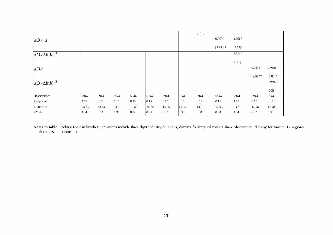
Table 7 sets out a number of robustness checks of these basic specifications.

Column 1 and 3 reproduce the previous results without and with interacted terms. Columns 2

and 4 add two skills measures to check that underlying skills were not driving both ∆O and

∆ln(Y/L). These skill measures are reported expenditure on training, a measure presumably of

10 Note that because we are including industry dummiesin the production function, lag labour productivity capture

the productivity gap between each plant and the three digit industry technological frontier (absorbed by the

15

changes in skill and reported fraction of staff educated to degree level or above, a measure

presumably of the level of skill that might affect changes in O or Y/L. Neither are significant or

affected the other coefficients.

Second, in columns 5 and 6 we re-specified the ∆O term to be just the wider innovation

term i.e. dropped the term in process innovation. Its sign was still positive but significance fell

somewhat. Third, in columns 7 and 8, we respecificed the ∆O term to use the “scale” of the

term, since we were concerned that simply a dummy does not distinguish well between firms

undergoing small and large ∆O. However, as noted above, one has to be very cautious here

since the scale of the variable is related to the success of the change which could of course be

endogenous to productivity growth. Nonetheless, in columns 7 and 8 we used ∆O as the

maximum of any of the answers to question 17.1. The effect is positive but not well determined.

In columns 9 and 10 we used the BBH standardised measure, namely the sum of the standardised

answers, which is itself then standardised.11 Both terms are positive and quite well determined.

Table 8 then explores these results by manufacturing and services with ln(Y/L)it-1

included and not. The main results suggest, interestingly, that the most statistically significant

effects of ∆O and its interactions are in services. One possibility is that manufacturing and

services simply have different elasticities, because software use is relatively more important in

services than in manufacturing. In our model, KIT proxies for hardware and O proxies for

software. This is reflected in a higher organisational change coefficient and a higher interaction

term of IT and organisational change.

5 Econometric implementation and results of ∆O equation

5.1 Econometric implementation

Our estimating equation for ∆O builds on (4) and can be written

1 1 21 1 22 1 23it it it it it I itO MSHARE SIZE GROWTH GE vβ β β β λ− − −∆ = ∆ + + + + + (7)

industry fixed effects).

11 Define STD(x) as (x-x*/σx) where x* is average x over the whole sample, then the variable is STD(ΣSTD(x)).

16

where ∆MSHARE i,t-1=(Li/LI)1998-(Li/LI)1997, SIZEt-1=lnY1998, GROWTHt-1= lnLi, 1998- lnLi, 1997,

recall that ∆O is defined between 2000 and 1998 and GE is a vector of four separate dummies

denoting global engagement taking the value one if a US MNE, a non-US/UK MNE, a UK MNE

and an exporter, where exporters are only those who export and not those who are UK MNEs. A

number of points are worth making. First, regarding measurement whilst we have Yi and Li in

1998 we only have Li in 1997.

Second, what is the rationale behind (7)? We think of it as a reduced form describing

two basic approaches to the determinants of O. The first might be to regard O as reflecting

knowledge capital. Grilliches’ (1979) model suggested modelling ∆Oi=f(Ri, Oi,, O_i) where R is

expenditure/effort into discovering new knowledge, and Oi and O_i the stocks of knowledge at

and outside the firm which firms can draw upon to make new discoveries. In this type of model

O at the frontier is unknown and requires some inputs to move towards it. Thus (7) might be

regarded as a reduced form describing this process. Competition forces firms to either invest in

more inputs to change O or to use such inputs more effectively. Larger firms might have more

knowledge stock upon which to draw or have economies of scale/scope in applying knowledge

to their production processes. Slow growing firms might be more inclined to invest in ∆O since

the opportunity cost of labour taken away from production to so invest is lower when sales are

lower. Or, they might be more inclined to invest in ∆O if changes, which might conceivably

involve job loss, are more acceptable to workers in growing companies (where employment

would grow by less than it would otherwise do, but at least not fall).12

A second way of viewing O is that organisational capital also includes the organisation of

work which can be summarised by the effort that workers apply to tasks. Thus changes in

organisational capital here are changes in work effort. In the knowledge capital model above

this arises from new knowledge about work practices. In this second view, the efficiency of

various work practices are known but implemented by firms to a greater or lesser extent. The

challenge is therefore to understand how different effort levels co-exist in equilibrium and how

they are affected by competition.

Competition likely increases effort and hence productivity in at least two settings, perfect

and imperfect competition. In Leamer (1999) there is perfect competition but two sectors,

capital and labour intensive. The price and productivity of capital increases with effort (since

12 The variable growth could be also capturing expectations of doing better in the future, hence it becomes

reasonable to introduce the organisational changes today because the (expected) discounted opportunity costs could be lower.

17

low effort means idle capital) and hence the capital intensive sector prefers high effort for which

it is prepared to pay high wages as compensation (whilst the labour intensive sector pays low

wages but demands low effort, with workers indifferent in equilibrium between the two

contracts). Effort rises in response to increased competition, here via a Stolper-Samuelson effect

from an exogenous lowing of product prices in the labour intensive sector.13

An alternative approach to modelling effort is under imperfect competition (see e.g.

Nickell, 1996, Haskel, 1991). Here workers value high wages and low effort and have some

labour market power and so are able to bargain with firms, who themselves have some product

market power. Tighter product market competition raises the marginal cost to workers of

demanding lower effort since consequent marginal reductions in employment are larger. Under

certain conditions, workers raise their effort.14 In this model effort might also vary with size and

growth if larger or growing firms are better able to bargain.

5.2 Results

Table 9 shows the results of estimating (7) (by probit since ∆Oi is a 1/0 variable, coefficients

reported are marginal effects). Note the number of observations is 5,944 as before but shows up

as 5,881 in the table since we include three-digit dummies that perfectly explain some of the

observations. Column 1 shows the results for manufacturing and services, excluding the GE

dummies and ln(Y/L)it-1. Larger and faster growing firms are both more likely to introduce ∆Oi.

The key variable for our purposes is the ∆MSHAREi, t-2 variable, here measured as the lagged

change in market share, which is negative and statistically significant. The negative term

suggests that firms who lost market share in the period 1997-1998 were more likely to introduce

∆Oi between 1998-2000. This effect when using lags is more revealing of the true causal effect

(which of course we cannot estimate without a natural experiment) since using current data

would likely induce a positive correlation since firms introducing ∆Oi likely grow market share.

Since the endogeneity bias likely biases the effect toward being positive, the true causal effect is

likely more negative than the negative effect that we find.

13 In this model all firms are the same, except for being in different sectors, and so firm market shares do not change,

which is what we use empirically here as a measure of competition. 14 The conditions essentially depend upon worker preferences over wages and effort: if workers marginal disutlity

from increases in effort is sufficiently large and their disutility from falls in wages is sufficiently small then workers might agree steep enough wage cuts in the face of increased competition to be able to take effort reductions too.

18

Column 2 enters the four GE dummies, US MNEs, non-US (but non-UK) MNEs, and UK

MNEs and the EXPORT dummy. The effects here are most interesting. First, the ∆MSHARE

term is hardly affected. Second, the coefficients on the dummies are greatest for US MNEs, and

then similar for other MNEs and exporters, with the omitted group being UK domestic firms.

This suggests that controlling for competition, nonUS firms are statistically less likely to

introduce ∆Oi than US firms. These effects are economically significant too, with US MNEs

15% (instead of 13%) more likely to introduce DO than, for example, UK domestic firms. Non

UK multinationals behave similar to those UK domestic firms that are exporters. .Finally, the lag

(labour) productivity term was always negative and significant, suggesting that firms below the

average labour productivity in the sector in the previous years were more likely to introduce

organisational changes in the following period. In other words, organisational changes are an

important transmission mechanism for the catching up process.15

The rest of the table shows these results for manufacturing and services and suggests the

DMSHARE and MNE results are robust (although the significance, but not the sign, of

DMSHARE falls slightly when the data is split between manufacturing and services). This

suggests a possible explanation for the difference in US and UK productivity performance in

recent periods: that UK firms, controlling for their type and competition, are less likely to

introduce organisational change.

5.3 IV

Table puts the findings on the effect of ∆O on productivity growth and the determinants of ∆O

together. Column 1 reports the IV estimate of the effect of ∆O on productivity growth in (6)

using the terms in (7) as instruments for ∆O (as the first stage F test and the Sargan test show,

these instruments are strong and valid). The coefficient, 0.0485 is similar to the OLS coefficient,

but poorly determined. Indeed, as the Hausman test reported in Table 10 shows, there is no

statistically significant difference between the OLS and IV results.16 Column 2 repeats this

exercise adding an interaction17 but finds similarly less well defined results.

15 This result only emerges in the conditional model. In the unconditional one there is actually a positive and

significant correlation between organisational change and lag labour productivity (see Table 2 column 3 and 4). 16 Note we are not claiming that ∆O is exogenous, but simply that with this current model which attempts to

endogenise ∆O , OLS and IV give, statistically speaking, the same results. 17 This also allow to add more instruments by interacting the original instrumental variables with IT investment.

19

Column 3 and 4 add ln(Y/L)it-1 to both (6) and (7). As before the coefficient on ∆O rises

in both magnitude and significance, with the effect of ∆O being to raise productivity growth by

8-10%. The Hausman test however still does not reject the hypothesis that the IV and OLS

coefficients are the same (with the exception of the test in column 3). Finally, given the results

of the Hausman tests, the last columns show SURE estimates of (6) and (7) (with and without

ln(Y/L)it-1). The coefficients are not much changed from the OLS results, although the

coefficient of . ∆O become more signficant, while the interaction is less signficant.

6 Conclusion and discussion

This paper has used panel data on productivity, ICT and organisational change in UK

establishments to examine the relationships between productivity growth, ICT and organisational

change. Consistent with the small number of other micro studies we find (a) ICT appears to

have high returns in a growth accounting sense when one omits ∆O, but when ∆O is included the

ICT returns are greatly reduced. (b) ICT and ∆O interact in their effect on productivity growth.

(c) there is no impact on productivity growth from ∆O and non-ICT investment. Some new

findings are (a), we find that ∆O is affected by competition and (b) US-owned firms are much

more likely to introduce ∆O relative to other MNEs and exporters who are more likely still

relative to UK domestic only firms. Of course one should be cautions about these results given

measurement error and the attendant difficulties of empirical work. But they suggest an

intriguing story explaining the lack of productivity growth following the IT revolution in the UK.

It is that productivity gains from IT depend upon organisational change, but that organisational

change is introduced less readily where there is less competitive pressure and less readily relative

to US firms. Quite why the latter is the case is something that deserves further investigation.

20

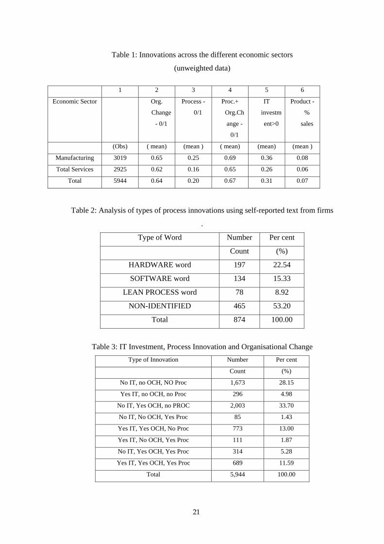
Table 1: Innovations across the different economic sectors

(unweighted data)

1 2 3 4 5 6

Economic Sector Org.

Change

- 0/1

Process -

0/1

Proc.+

Org.Ch

ange -

0/1

IT

investm

ent>0

Product -

%

sales

(Obs) ( mean) (mean ) ( mean) (mean) (mean )

Manufacturing 3019 0.65 0.25 0.69 0.36 0.08

Total Services 2925 0.62 0.16 0.65 0.26 0.06

Total 5944 0.64 0.20 0.67 0.31 0.07

Table 2: Analysis of types of process innovations using self-reported text from firms

.

Type of Word Number Per cent

Count (%)

HARDWARE word 197 22.54

SOFTWARE word 134 15.33

LEAN PROCESS word 78 8.92

NON-IDENTIFIED 465 53.20

Total 874 100.00

Table 3: IT Investment, Process Innovation and Organisational Change Type of Innovation Number Per cent

Count (%)

No IT, no OCH, NO Proc 1,673 28.15

Yes IT, no OCH, no Proc 296 4.98

No IT, Yes OCH, no PROC 2,003 33.70

No IT, No OCH, Yes Proc 85 1.43

Yes IT, Yes OCH, No Proc 773 13.00

Yes IT, No OCH, Yes Proc 111 1.87

No IT, Yes OCH, Yes Proc 314 5.28

Yes IT, Yes OCH, Yes Proc 689 11.59

Total 5,944 100.00

21

Table 4: Innovations and firm’s characteristics (after demeaning)

Size (t-1)

LP (t-1)

ICT

DMS(t-1)

Small Large Low High Low High Low High

Obs 3253 2691 3138 2806 4853 1091 3328 2616

Product - % sales -0.010 0.012 -0.006 0.007 -0.016 0.073 -0.003 0.003

Process - 0/1 -0.042 0.051 -0.004 0.005 -0.056 0.250 -0.015 0.019

Org. Change - 0/1 -0.074 0.089 -0.018 0.021 -0.033 0.146 -0.022 0.028

Proc.+ Org.Change –

0/1

-0.072 0.088 -0.018 0.021 -0.040 0.176 -0.023 0.029

Note: In order to buld this table we have first controlled for 3 digit SIC fixed effects and then we compute a dummy variable if the firm was above the sectoral average.

Table 5: Innovations across firm’s ownership status OWNERSHIP Product -

%

sales

Process -

0/1

Org.

Chang

e - 0/1

Proc.+

Org.Cha

nge - 0/1

(Obs) (mean) (mean ) (mean) (mean )

Domestic 4845 0.060 0.184 0.601 0.634

US MNE 191 0.105 0.246 0.843 0.890

No US MNE 413 0.111 0.266 0.782 0.809

UK MNE 495 0.094 0.303 0.776 0.804

Total 5944 0.068 0.202 0.636 0.669

22

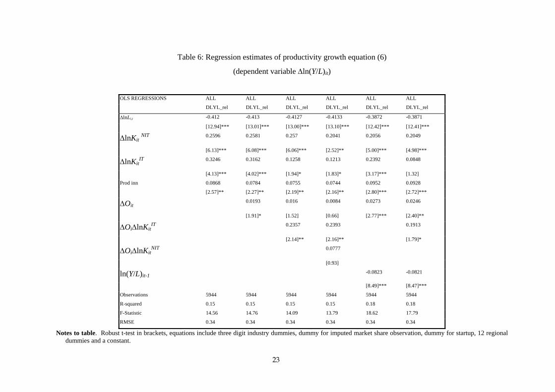
Table 6: Regression estimates of productivity growth equation (6)

(dependent variable ∆ln(Y/L)it)

OLS REGRESSIONS ALL ALL ALL ALL ALL ALL

DLYL_rel DLYL_rel DLYL_rel DLYL_rel DLYL_rel DLYL_rel

∆lnLi,t -0.412 -0.413 -0.4127 -0.4133 -0.3872 -0.3871

[12.94]*** [13.01]*** [13.00]*** [13.10]*** [12.42]*** [12.41]***

∆lnKit NIT 0.2596 0.2581 0.257 0.2041 0.2056 0.2049

[6.13]*** [6.08]*** [6.06]*** [2.52]** [5.00]*** [4.98]***

∆lnKitIT 0.3246 0.3162 0.1258 0.1213 0.2392 0.0848

[4.13]*** [4.02]*** [1.94]* [1.83]* [3.17]*** [1.32]

Prod inn 0.0868 0.0784 0.0755 0.0744 0.0952 0.0928

[2.57]** [2.27]** [2.19]** [2.16]** [2.80]*** [2.72]***

∆Oit 0.0193 0.016 0.0084 0.0273 0.0246

[1.91]* [1.52] [0.66] [2.77]*** [2.40]**

∆Oi∆lnKitIT

0.2357 0.2393 0.1913

[2.14]** [2.16]** [1.79]*

∆Oi∆lnKitNIT

0.0777

[0.93]

ln(Y/L)it-1 -0.0823 -0.0821

[8.49]*** [8.47]***

Observations 5944 5944 5944 5944 5944 5944

R-squared 0.15 0.15 0.15 0.15 0.18 0.18

F-Statistic 14.56 14.76 14.09 13.79 18.62 17.79

RMSE 0.34 0.34 0.34 0.34 0.34 0.34

Notes to table. Robust t-test in brackets, equations include three digit industry dummies, dummy for imputed market share observation, dummy for startup, 12 regional dummies and a constant.

23

Table 7: Robustness checks on Table 6

(dependent variable ∆ln(Y/L)it) Base Training Base Training no Proc no Proc Only OrgB Only_OrgC Scale BBH Scale BBH Scale C Scale

DLYL_rel DLYL_rel DLYL_rel DLYL_rel DLYL_rel DLYL_rel DLYL_rel DLYL_rel DLYL_rel DLYL_rel DLYL_rel DLYL_rel

∆lnLi,t -0.413 -0.4131 -0.4127 -0.4129 -0.4129 -0.4129 -0.4123 -0.4123 -0.4131 -0.413 -0.4131 -0.413

[13.01]*** [13.00]***[13.01]*** [13.00]*** [13.01]*** [13.00]*** [12.97]*** [12.99]***[12.97]*** [12.99]*** [12.99]*** [12.99]***

∆lnKit NIT 0.2581 0.2577 0.257 0.2566 0.2586 0.2583 0.2591 0.2591 0.2563 0.2563 0.2562 0.2562

[6.08]*** [6.07]*** [6.06]*** [6.05]*** [6.09]*** [6.08]*** [6.10]*** [6.10]*** [6.01]*** [6.01]*** [6.01]*** [6.01]***

∆lnKitIT 0.3162 0.3221 0.1258 0.1305 0.3198 0.2433 0.3228 0.306 0.3141 0.3048 0.3139 0.292

[4.02]*** [4.06]*** [1.94]* [2.01]** [4.07]*** [2.73]*** [4.11]*** [3.85]*** [3.96]*** [4.02]*** [3.96]*** [3.39]***

Prod inn 0.0784 0.0827 0.0755 0.0799 0.0801 0.0792 0.0845 0.0845 0.076 0.0759 0.0757 0.0757

[2.27]** [2.32]** [2.19]** [2.24]** [2.33]** [2.30]** [2.47]** [2.47]** [2.21]** [2.21]** [2.21]** [2.20]**

∆Oit0.0193 0.0207 0.016 0.0174

[1.91]* [2.01]** [1.52] [1.63]

∆Oit∆lnKitIT 0.2357 0.2373

[2.14]** [2.15]**

train_rel -0.009 -0.0093

[0.70] [0.72]

skills_rel -0.0054 -0.0054

[0.19] [0.18]

∆Oit′ 0.0168 0.0147

[1.73]* [1.45]

∆Oit′∆lnKitIT 0.1071

0.81] [

∆Oit′ 0.0064 0.0058

[0.70] [0.59]


24

0.20] [

∆Oit′ rel 0.0091 0.0087

[1.98]** [1.77]*


0.29] [

∆Oit′ 0.0375 0.0355

[2.02]** [1.80]*


.33] [0

Observations 5944 5944 5944 5944 5944 5944 5944 5944 5944 5944 5944 5944

R-squared 0.15 0.15 0.15 0.15 0.15 0.15 0.15 0.15 0.15 0.15 0.15 0.15

F-Statistic 14.76 13.43 14.09 12.88 14.74 14.05 14.36 13.81 14.45 13.77 14.46 13.78

RMSE 0.34 0.34 0.34 0.34 0.34 0.34 0.34 0.34 0.34 0.34 0.34 0.34

Notes to table. Robust t-test in brackets, equations include three digit industry dummies, dummy for imputed market share observation, dummy for startup, 12 regional

dummies and a constant.

25

Table 8: Regression estimates of productivity growth equation (6) for manufacturing and services

(dependent variable ∆ln(Y/L)it) OLS REGRESSIONS BY SECTOR Manuf Svs Manuf Svs Manuf Svs Manuf Svs

DLYL_rel DLYL_rel DLYL_rel DLYL_rel DLYL_rel DLYL_rel DLYL_rel DLYL_rel

∆lnLi,t -0.3527 -0.463 -0.3531 -0.4621 -0.3104 -0.4467 -0.3107 -0.4461

[6.60]*** [12.20]*** [6.60]*** [12.17]*** [6.05]*** [11.95]*** [6.05]*** [11.92]***

∆lnKit NIT 0.2554 0.2588 0.2543 0.2578 0.1776 0.2211 0.1767 0.2206

[3.56]*** [5.11]*** [3.55]*** [5.09]*** [2.68]*** [4.44]*** [2.67]*** [4.42]***

∆lnKitIT 0.2584 0.4022 0.0982 0.144 0.1748 0.3264 0.0386 0.1177

[2.53]** [3.37]*** [1.18] [1.18] [1.89]* [2.75]*** [0.49] [0.94]

Prod inn 0.1062 0.0534 0.1036 0.0502 0.1246 0.0676 0.1224 0.0649

[2.61]*** [0.96] [2.55]** [0.90] [3.22]*** [1.22] [3.17]*** [1.16]

∆Oit-0.0063 0.0432 -0.0098 0.0396 0.0116 0.0467 0.0087 0.0438

[0.45] [2.96]*** [0.65] [2.66]*** [0.87] [3.24]*** [0.62] [2.97]***

∆Oi∆lnKitIT 0.1957 0.3275 0.1664 0.2654

[1.39] [1.77]* [1.30] [1.42]

ln(Y/L)it-1 -0.1344 -0.0532 -0.1343 -0.0529

[7.19]*** [5.22]*** [7.19]*** [5.18]***

Constant 0.3128 0.4258 0.3126 0.4254 0.2438 0.4048 0.2437 0.4046

[3.22]*** [4.36]*** [3.22]*** [4.35]*** [3.02]*** [4.24]*** [3.02]*** [4.24]***

Observations 3019 2925 3019 2925 3019 2925 3019 2925

R-squared 0.13 0.17 0.13 0.17 0.2 0.18 0.2 0.18

F-Statistic 6.66 12.07 6.38 11.61 10.79 12.36 10.39 11.87

RMSE 0.3 0.38 0.3 0.38 0.29 0.37 0.29 0.37


26

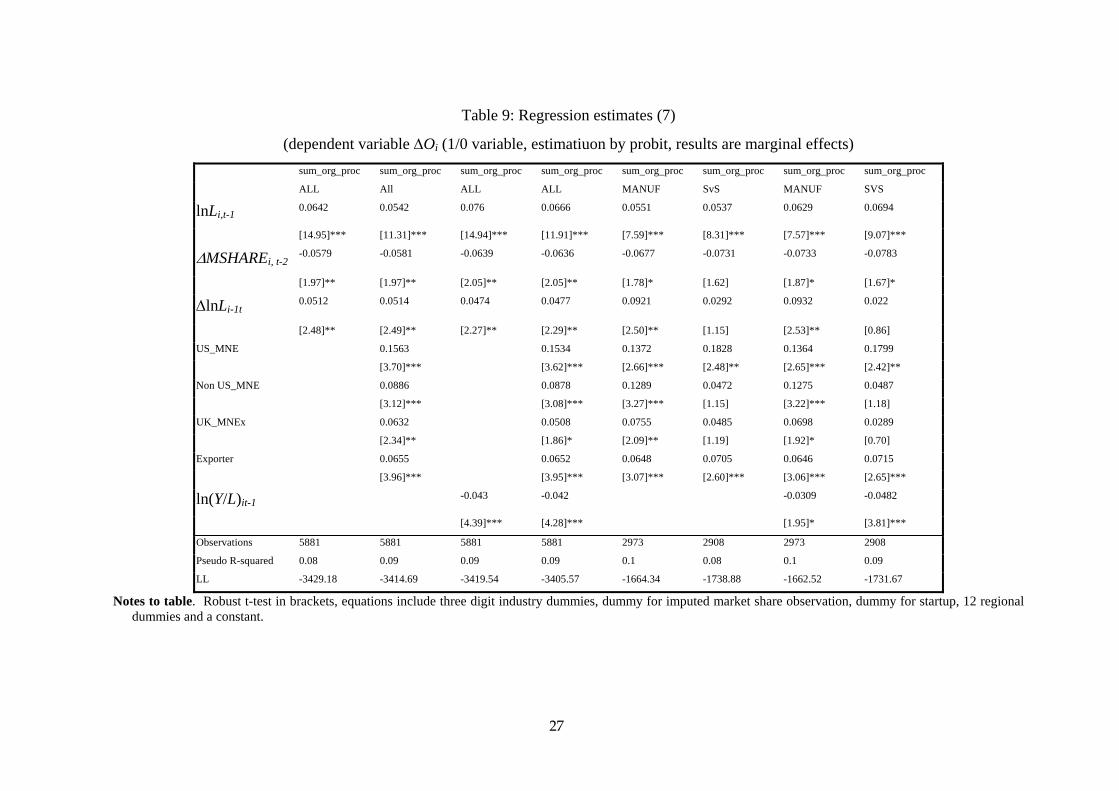
Table 9: Regression estimates (7)

(dependent variable ∆Oi (1/0 variable, estimatiuon by probit, results are marginal effects) sum_org_proc sum_org_proc sum_org_proc sum_org_proc sum_org_proc sum_org_proc sum_org_proc sum_org_proc

ALL All ALL ALL MANUF SvS MANUF SVS

lnLi,t-10.0642 0.0542 0.076 0.0666 0.0551 0.0537 0.0629 0.0694

[14.95]*** [11.31]*** [14.94]*** [11.91]*** [7.59]*** [8.31]*** [7.57]*** [9.07]***

∆MSHAREi, t-2-0.0579 -0.0581 -0.0639 -0.0636 -0.0677 -0.0731 -0.0733 -0.0783

[1.97]** [1.97]** [2.05]** [2.05]** [1.78]* [1.62] [1.87]* [1.67]*

∆lnLi-1t0.0512 0.0514 0.0474 0.0477 0.0921 0.0292 0.0932 0.022

[2.48]** [2.49]** [2.27]** [2.29]** [2.50]** [1.15] [2.53]** [0.86]

US_MNE 0.1563 0.1534 0.1372 0.1828 0.1364 0.1799

[3.70]*** [3.62]*** [2.66]*** [2.48]** [2.65]*** [2.42]**

Non US_MNE 0.0886 0.0878 0.1289 0.0472 0.1275 0.0487

[3.12]*** [3.08]*** [3.27]*** [1.15] [3.22]*** [1.18]

UK_MNEx 0.0632 0.0508 0.0755 0.0485 0.0698 0.0289

[2.34]** [1.86]* [2.09]** [1.19] [1.92]* [0.70]

Exporter 0.0655 0.0652 0.0648 0.0705 0.0646 0.0715

[3.96]*** [3.95]*** [3.07]*** [2.60]*** [3.06]*** [2.65]***

ln(Y/L)it-1 -0.043 -0.042 -0.0309 -0.0482

[4.39]*** [4.28]*** [1.95]* [3.81]***

Observations 5881 5881 5881 5881 2973 2908 2973 2908

Pseudo R-squared 0.08 0.09 0.09 0.09 0.1 0.08 0.1 0.09

LL -3429.18 -3414.69 -3419.54 -3405.57 -1664.34 -1738.88 -1662.52 -1731.67


27

Table 10: Regression estimates of productivity growth equation (6) by IV and system estimation

(dependent variable ∆ln(Y/L)it, only coefficient on ∆O and ∆O•∆KIT reported)

IV IV IV IV SURE SURE SURE SURE

RESULTS RESULTS RESULTS RESULTS RESULTS RESULTS RESULTS RESULTS

∆Oit0.0485 0.0408 0.1081 0.0859 0.0197 0.0165 0.027 0.0245

[0.98] [0.80] [2.11]** [1.60] [2.02]** [1.66]* [2.81]*** [2.49]**

∆Oi∆lnKitNIT 0.2984 0.2352 0.2204 0.1766

[1.06] [0.69] [1.60] [1.30]

Sargan 9.33 10.64 10.41* 12.15

hausman 0.38 0.27 1.71* 1.08

F-First Step (org_change) 39.06*** 21.53*** 33.91*** 18.75***

F-First Step (Interaction) 110.28*** 95.74***

LYL_lag No No Yes Yes No No Yes Yes


28

7. References Basu, S., J.G. Fernald, N. Oulton, and S. Srinivasan (2003): “The case of Missing Productivity

Growth: Or, Does Information Technology Explain why Productivity Accelerated in the US but not the UK”, NBER Working Paper 10010, October

Black, S. and L. M. Lynch (2001): "How to compete: The Impact of Workplace Practices and

Information Technology on Productivity growth” The Review of Economics and Statistics V 83(3) 434-445.

Black, S. and L. M. Lynch (2003): "What's driving the new economy?: the benefits of workplace

innovation," Working Papers in Applied Economic Theory 2003-23, Federal Reserve Bank of San Francisco.

Boning, B., Ichniowski and K. Shaw (2001): “Opportunity Counts: Teams and the Effectiveness

of Production Incentives”, NBER Working Paper 8306 Bresnahan, T. F., Brynjolfsson, E. and Hitt, L. M. (2002):. "Information Technology, Workplace

Organization, And The Demand For Skilled Labor: Firm-Level Evidence," The Quarterly Journal of Economics, MIT Press, vol. 117(1), pages 339-376

Brynjolfsson, E. and Hitt, L. M. (2003):. "Computing Productivity: Firm level evidence” The

Review of Economics and Statistics, MIT Press, vol. 85(4), pages 793-808 Brown, C. and Medoff, J. (1978): ‘Trade Unions in the Production Process’, Journal of Political

Economy, Vol.86, pp.355-378. Clark, K. (1984): “Unionisation and Firm Performance: The Impact on Profits, Growth and

Productivity”, American Economic Review, Vol.74(5), December, pp.893-919. Chiara Criscuolo and Ralf Martin, (2004), "Multinationals and US Productivity Leadership:

Evidence from Great Britain” OECD Science, Technology and Industry Department Working Papers (2004)5, OECD Science, Technology and Industry Department

Criscuolo C., Haskel J. and Martin R., (2003): “Building the evidence base for productivity

policy using business data linking”, Economic Trends 600 November 2003, pp.39-51, available at < www.statistics.gov.uk/articles/economic_trends/ETNov03Haskel.pdf>.

Freeman, R. and Medoff, J. (1984): What do Unions do?, Basic Books: New York. Griliches, Z. (1979): “Issues in Assessing the Contribution of Research and Development to

Productivity Growth”, Bell Journal of Economics v10, n1 (Spr. 1979): 92-116 Disney, R., Haskel, J. and Heden Y. (2003): “ Reestructuring and Productivity Growth in UK

Manufacturing”, Economic Journal v113, 489, 669-94 Haskel, Jonathan, 1991. "Imperfect Competition, Work Practices and Productivity Growth,"

Oxford Bulletin of Economics and Statistics, vol. 53(3), pages 265-79.

29

http://www.statistics.gov.uk/articles/economic_trends/ETNov03Haskel.pdf>

Ichniowski ,C. and Shaw, K. (2003): "Beyond Incentive Pay: Insiders' Estimates of the Value of Complementary Human Resource Management Practices," Journal of Economic Perspectives, American Economic Association, vol. 17(1), pages 155-180.

Leamer, E.E. (1999), “Effort, Wages and the International Division of Labor," Journal of

Political Economy, Vol. 107, Number 6, Part 1, December, 1999, 1127-1163 Nickell, S. (1996): “Competition and Corporate Performance”, Journal of Political Economy

v104, n4, 724-46 Nickell, S.; Nicolitsas, D. and Patterson, M (2001): “Does Doing Badly Encourage Management

Innovation”, Oxford Bulletin of Economics and Statistics V63, n1, 5-28 Oulton, N. (1998), “Investment, Capital and Foreign Ownership in UK Manufacturing”, NIESR

Discussion Paper No. 141. Vaze, P.(2003), “Estimates of the volume of capital services”, Economic Trends 600, November

30

information technology, organisational change and

Documents