Università degli Studi di MilanoMaster Degree in Computer Science

Information Management course

Teacher: Alberto Ceselli

Lecture 08: 28/10/2015

2

Data Mining: Methods and

Models

— Chapter 1 —

Daniel T. Larose©2006 John Wiley and Sons

33

Data (Dimensionality) Reduction

In large datasets it is unlikely that all attributes are independent: multicollinearity

Worse mining quality: Instability in multiple regression (significant overall, but

poor wrt significant attributes) Overemphasize particular attributes (multiple counts) Violates principle of parsimony (too many unnecessary

predictors in a relation with a response var) Curse of dimensionality:

Sample size needed to fit a multivariate function grows exponentially with number of attributes

e.g. in 1-dimensional distrib. 68% of normally distributed values lie between -1 and 1; in 10-dimensional distrib. only 0.02% within the radius 1 hypersphere

4

Recall: Visually Evaluating Correlation

Scatter plots showing the similarity from –1 to 1.

A minimal approach: user defined composites

Sometimes correlation is known to the data analyst or evident from data

Then, nothing forbids to aggregate attributes by hand!

Example: say you have a “house” dataset then housing median age, total rooms, total

bedrooms and population can be expected to be strongly correlated as “block group size”

replace these four attributes with a new attribute, that is the average of them(possibly after normalization)

Xm+1i = (X1

i + X2i + X3

i + X4i) / 4

6

Parametric Data Reduction: Regression and Log-Linear Models

Linear regression Data modeled to fit a straight line Often uses the least-square method to fit the

line Multiple regression

Allows a “response” variable Y to be modeled as a linear function of multidimensional “predictor” feature (variable) vector X

Log-linear model Approximates discrete multidimensional

probability distributions

7

Regression Analysis

Regression analysis: A collective name for

techniques for the modeling and analysis

of numerical data consisting of values of a

dependent variable (also called

response variable or measurement) and

of one or more independent variables

(aka. explanatory variables or

predictors)

The parameters are estimated so as to

give a "best fit" of the data

Most commonly the best fit is evaluated

by using the least squares method, but

other criteria have also been used

Used for prediction (including forecasting of time-series data), inference, hypothesis testing, and modeling of causal relationships

y

x

y = x + 1

X1

Y1

Y1’

8

Linear regression: Y = w X + b

Two regression coefficients, w and b, specify the line and are to be estimated by using the data at hand

Using the least squares criterion to the known values of Y1,

Y2, …, X1, X2, ….

Multiple regression: Y = b0 + b1 X1 + b2 X2

Many nonlinear functions can be transformed as above

Log-linear models:

Approximate discrete multidimensional prob. distributions

Estimate the probability of each point (tuple) in a multi-dimensional space for a set of discretized attributes, based on a smaller subset of dimensional combinations

Useful for dimensionality reduction and data smoothing

Regress Analysis and Log-Linear Models

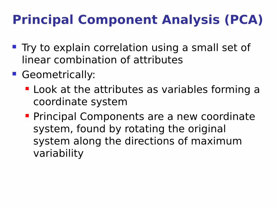
Principal Component Analysis (PCA)

Try to explain correlation using a small set of linear combination of attributes

Geometrically: Look at the attributes as variables forming a

coordinate system Principal Components are a new coordinate

system, found by rotating the original system along the directions of maximum variability

PCA – Step 1: preprocess data

Notation (review): Dataset with n rows and m columns Attributes (columns): Xj

Mean of each attrib:

Variance of each attrib:

Covariance between two attrib:

Correlation coefficient:

μ j=1n∑i=1

n

X ij

σ jj2=

1n∑i=1

n

(X ij−μ j)

2

σ kj2=

1n∑i=1

n

(X ik−μk )⋅(X i

j−μ j)

rkj=σ kj

2

σ kk σ jj

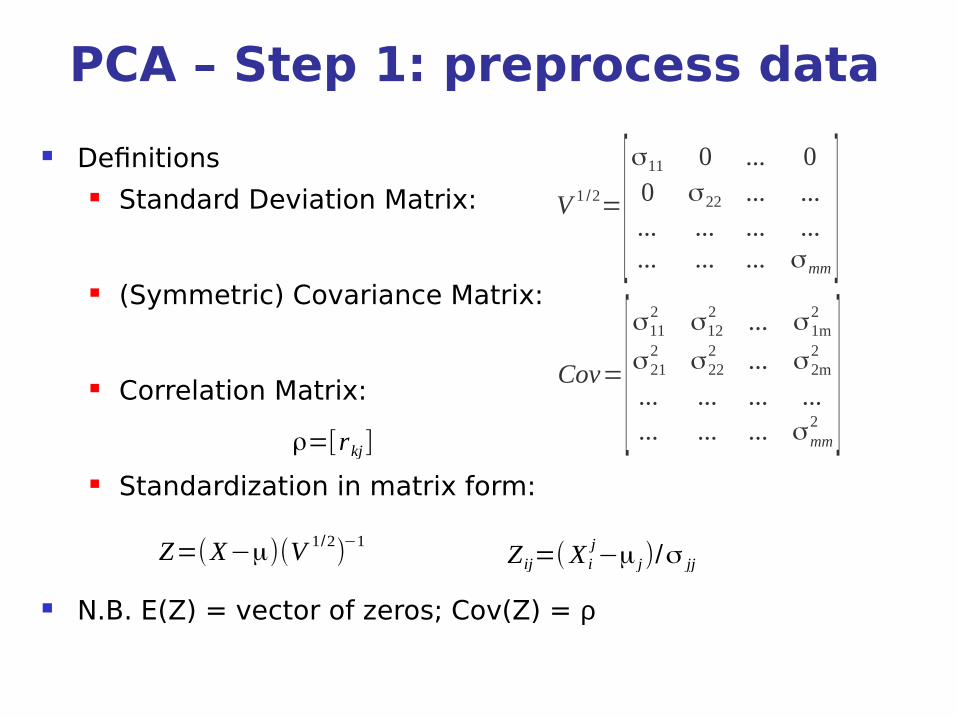
PCA – Step 1: preprocess data

Definitions Standard Deviation Matrix:

(Symmetric) Covariance Matrix:

Correlation Matrix:

Standardization in matrix form:

N.B. E(Z) = vector of zeros; Cov(Z) = ρ

V 1 /2=[σ11 0 ... 00 σ22 ... ...... ... ... ...... ... ... σmm

]Cov=[

σ112 σ12

2 ... σ1m2

σ212 σ22

2 ... σ2m2

... ... ... ...

... ... ... σmm2 ]

Z=(X−μ)(V 1/2)−1

Zij=(X ij−μ j)/σ jj

ρ=[rkj ]

PCA – Step 2: compute eigenvalues and eigenvectors

Eigenvalues of (mxm matrix) ρ are scalars λ1 ... λm such that det(ρ – λI) = 0

Given a matrix ρ and its eigenvalue λj, ej is a corresponding (mx1) eigenvector if ρ ej = λjej

Spectral theorem / symmetric eigenvalue decomposition (for symmetric ρ)

We are interested in eigenvalues / eigenvectors of the correlation matrix

ρ=∑ j=1

mλ j e

j(e j

)T

PCA – Step 3: compute principal components

Consider the original (standardized, nxm) matrix Z, with columns Zj

Consider the (nx1 column) vectors Yj = Z ej

e.g. Y1 = e11 Z1 + e1

2 Z2 + … + e1m Zm

Sort Yj by value of variance: Var(Yj) = (ej)T ρ (ej)

Then1)Start with an empty sequence of principal components

2)Select the vector ej that

1)maximizes Var(Yj)

2)Is independent from all selected components

3)Goto (2)

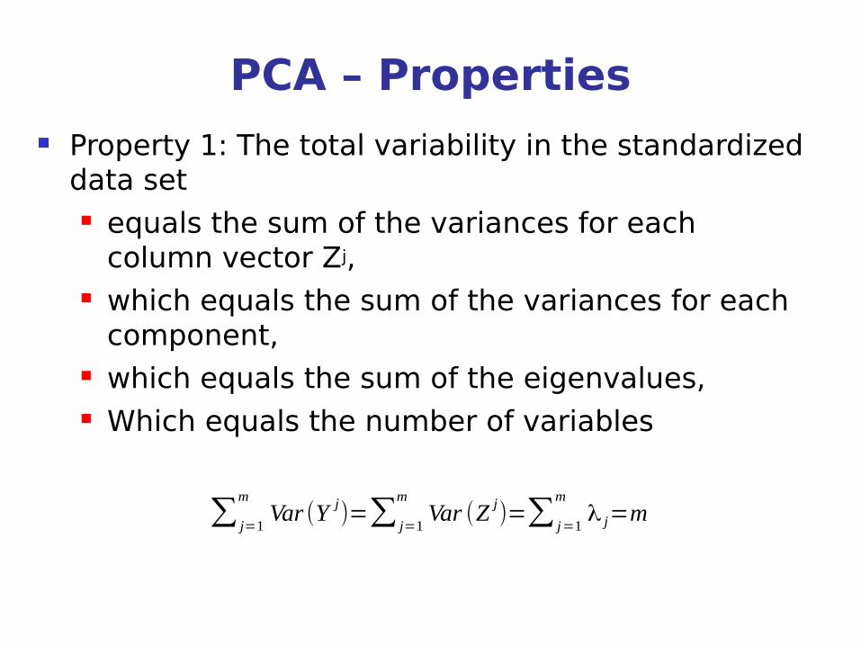
PCA – Properties Property 1: The total variability in the standardized

data set equals the sum of the variances for each

column vector Zj, which equals the sum of the variances for each

component, which equals the sum of the eigenvalues, Which equals the number of variables

∑ j=1

m

Var (Y j)=∑ j=1

m

Var (Z j)=∑ j=1

m

λ j=m

PCA – Properties Property 2: The partial correlation between a given

component and a given variable is a function of an eigenvector and an eigenvalue. In particular, Corr(Yk, Zj) = ek

j sqrt(λk)

Property 3: The proportion of the total variability in Z that is explained by the jth principal component is the ratio of the jth eigenvalue to the number of variables, that is the ratio λj/m

PCA – Experiment on real data Open R and read “cadata.txt” Keep first attribute (say 0) as response, remaining

ones as predictors Know Your Data: Barplot and scatterplot attributes Normalize Data Scatterplot normalized data Compute correlation matrix Compute eigenvalues and eigenvectors Compute components (eigenvectors) – attribute

correlation matrix Compute cumulative variance explained by

principal components

PCA – Experiment on real data Details on the dataset:

Block groups of houses (1990 California census) Response: Median house value Predictors:

1)Median income2)Housing median age3)Total rooms4)Total bedrooms5)Population6)Households7)Latitude8)Longitude

PCA – Step 4: choose components How many components should we extract?

Eigenvalue criterion Keep components having λ>1 (they “explain”

more than 1 attribute) Proportion of the variance explained

Fix a coefficient of determination r Choose the min. number of components to

reach a cumulative variance > r Scree plot Criterion

(try to barplot eigenvalues) Stop just prior to “tailing off”

Communality Criterion

PCA – Profiling the components Look at principal components:

Comp. 1 is “explaining” attributes 3, 4, 5 and 6

→ block group size? Comp. 2 is “explaining” attributes 7 and 8

→ geography? Comp. 3 is “explaining” attribute 1

→ salary? Comp. 4 ???

Compare factor scores of components 3 and 4 with attributes 1 and 2

PCA – Communality of attributes Def: communality of an (original) attribute j is the

sum of squared principal component weights for that attribute.

When we consider only the first p principal components:

k(p,j) = corr(1,j)2 + corr(2,j)2 + … + corr(p,j)2

Interpretation: communality is the fraction of variability of an attribute “extracted” by the selected principal components

Rule of thumb: communality < 0.5 is low! Experiment: compute communality for attribute 2

when 3 or 4 components are selected

PCA – Final choice of components Eigenvalue criterion did not exclude component 4

(and it tends to underestimate when number of attributes is small)

Proportion of variance criterion suggests to keep component 4

Scree criterion suggests not to exceed 4 components

Minimum communality suggests to keep component 4 to keep attribute 2 in the analysis

→ Let's keep 4 components