information, computation, and communication

ICC Module Computation Lesson 2 – Computation & Algorithms II

1

Information, Computation, and Communication

Algorithm 2


2

§ Recursion§ Complexity of a recursive algorithm§ Dynamic Programming§ (Binary Search « Recherche dichotomique »)

Topics

Understanding a Recurive Algorithm

A. 5B. 8C. 24D. 32

What is the output if L={5,8,6,10,3}?


4

Complexity

Algo1({5,8,6,10,3})

Algo1({8,6,10,3})

Algo1({6,10,3})

Height? Cost?

n+1

Algo1({10,3})

Algo1({3})

Algo1({}) 3

--”--

--”--

--”--

--”--

∼ 10

T(n)=10・n + 3 = Θ(n)T(n)= T(n-1) + 10T(0) = 3


5

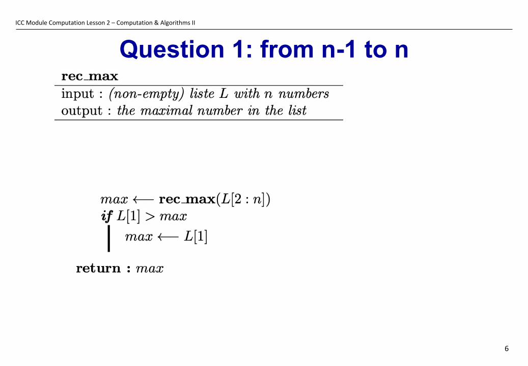
§ Find the largest number in a list• Input: a list L with n numbers• Output: the largest number in this list

§ Idea of recursion: • Use a solution of a smaller problem (a shorter list)

§ You need to answer two questions:1. Assume we are given the largest element in the list

L[2:n] (list of length n-1), how would we compute the largest element of the list L[1:n]?

2. What is the termination condition? What is the largest element of a list of size 1?

Writing a Recursive Algorithm


6

Question 1: from n-1 to n


7

Question 2: Termination

Find Max (Recursively)

A. Θ(log(n))B. Θ(n)C. Θ(n2)D. Θ(2n)

What is the complexity of this algorithm?


9

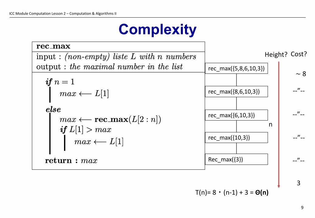
Complexity

rec_max({5,8,6,10,3})

rec_max({8,6,10,3})

rec_max({6,10,3})

Height? Cost?

n

rec_max({10,3})

Rec_max({3})

3

--”--

--”--

--”--

--”--

∼ 8

T(n)= 8・(n-1) + 3 = Θ(n)


10

§ The recursive solution is not always the only solution and rarely the most efficient...

§ ...but it is sometimes much simpler and more practical to implement !

§ Examples : sorting, processing of recursive data structures (e.g. trees, graphs, ...), ...

Recursion or Not?


11

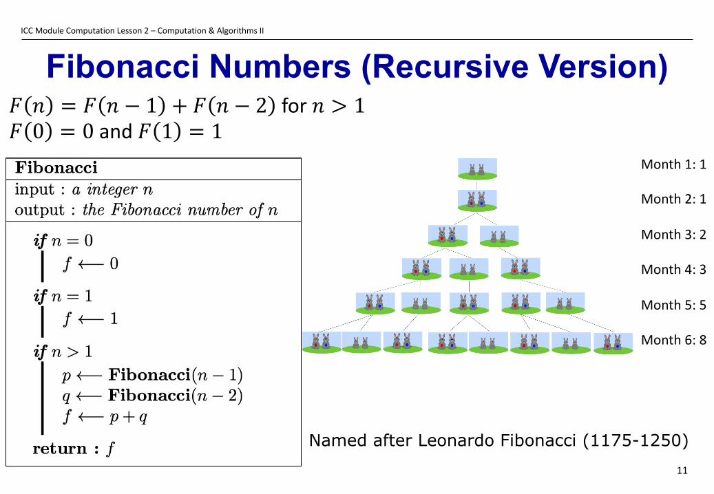
Fibonacci Numbers (Recursive Version)

Month 1: 1

Month 2: 1

Month 3: 2

Month 4: 3

Month 5: 5

Month 6: 8

Named after Leonardo Fibonacci (1175-1250)

𝐹 𝑛 = 𝐹 𝑛 − 1 + 𝐹 𝑛 − 2 for 𝑛 > 1𝐹 0 = 0 and 𝐹 1 = 1


12

Fibonacci Numbers in Nature

In these pictures there are 55 curves of seeds spiraling to the left as you go outwards and 34 spirals of seeds spiraling to the right. A little further towards the center you can count 34 spirals to the left and 21 spirals to the right. These pairs of numbers are (almost always) neighbors in the Fibonacci series.

The lengths of the squares describing naturally appear spirals are often Fibonacci numbers.1 1

2 3

58

13

https://plus.maths.org/content/life-and-numbers-fibonacci

Number of ancestors of a drone (a male honey bee) is a sum of Fibonacci number.

https://plus.maths.org/content/life-and-numbers-fibonacci


13

Fibonacci Recursive

F(5) = F(4)+F(3)

F(4) = F(3)+F(2) F(3) = F(2)+F(1)

F(3) = F(2)+F(1) F(2) = F(1)+F(0) F(2) = F(1)+F(0) F(1)

F(2) = F(1)+F(0) F(1) F(1) F(0)F(1) F(0)

F(1) F(0)

Height? Cost?

1

2

4

6

2

In each box in this tree we have to performance a constant number of instructions.1. How many boxes (function calls) are in this tree?2. How high is the tree? The height is n

> ∑!"#!"#$ 2! = 2

!%#$ − 1 = Ω(2

!$) lower bound

< ∑!"#$ 2! = 2$%& − 1 = 𝑂 2$ upper bound

𝐹 𝑛 = 𝐹 𝑛 − 1 + 𝐹 𝑛 − 2 for 𝑛 > 1𝐹 0 = 0 and 𝐹 1 = 1


14

§ Complexity F(n)?Exponential in n

§ Is there a better solution?

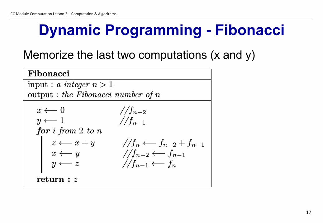
Idea: do not perform the same calculation many times but store the already calculated value for later use

Fibonacci Recursive


15

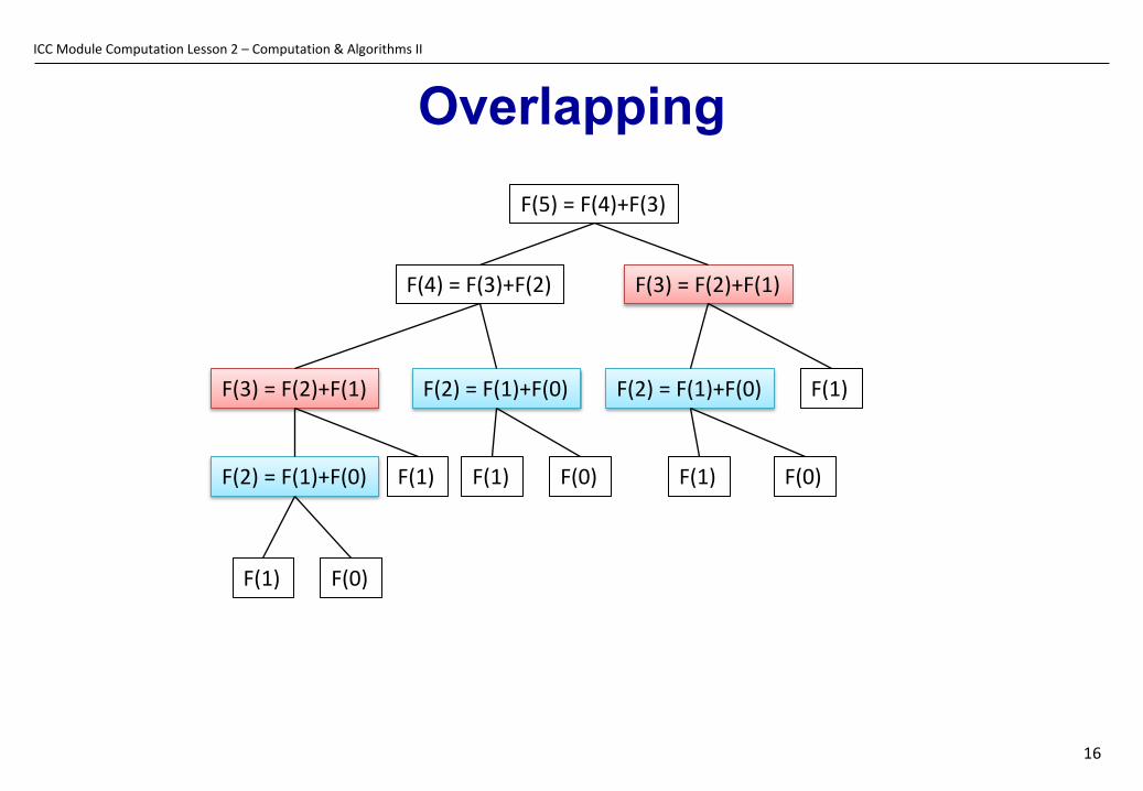
§ Dynamic programming is strategy to solve problems.• It applies to problems for which we can find an optimal

solution by breaking it down into smaller optimal overlapping sub-problems in a recursive manner.

• To solve such problems efficiently we memorize the solutions of sub-problems to avoid re-computation.

§ If the sub-problems are not overlapping the solving strategy is called ”divide and conquer” (like in binary search « Recherche dichotomique »).

Dynamic Programming


16

OverlappingF(5) = F(4)+F(3)

F(4) = F(3)+F(2) F(3) = F(2)+F(1)

F(3) = F(2)+F(1) F(2) = F(1)+F(0) F(2) = F(1)+F(0) F(1)

F(2) = F(1)+F(0) F(1) F(1) F(0)F(1) F(0)

F(1) F(0)


17

Memorize the last two computations (x and y)

Dynamic Programming - Fibonacci

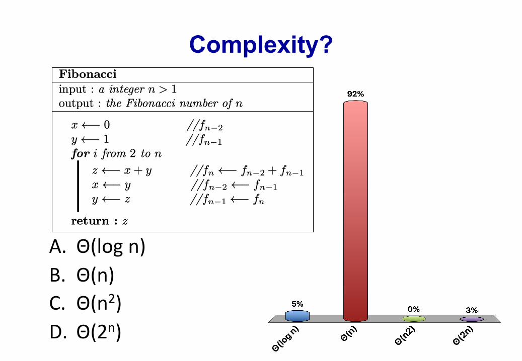
Complexity?

A. Θ(log n)B. Θ(n)C. Θ(n2)D. Θ(2n)


19

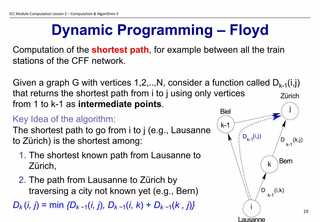
Computation of the shortest path, for example between all the train stations of the CFF network.

Given a graph G with vertices 1,2,..,N, consider a function called Dk-1(i,j) that returns the shortest path from i to j using only vertices from 1 to k-1 as intermediate points.

Dynamic Programming – Floyd

Key Idea of the algorithm:The shortest path to go from i to j (e.g., Lausanne to Zürich) is the shortest among:

1. The shortest known path from Lausanne toZürich,

2. The path from Lausanne to Zürich by traversing a city not known yet (e.g., Bern)

Dk (i, j) = min {Dk −1(i, j), Dk −1(i, k) + Dk −1(k , j)}

D (k,j)k-1

Dk-1(i,j)

D (i,k)k-1

Zürich

jBiel

k-1

i

Lausanne

k Bern


20

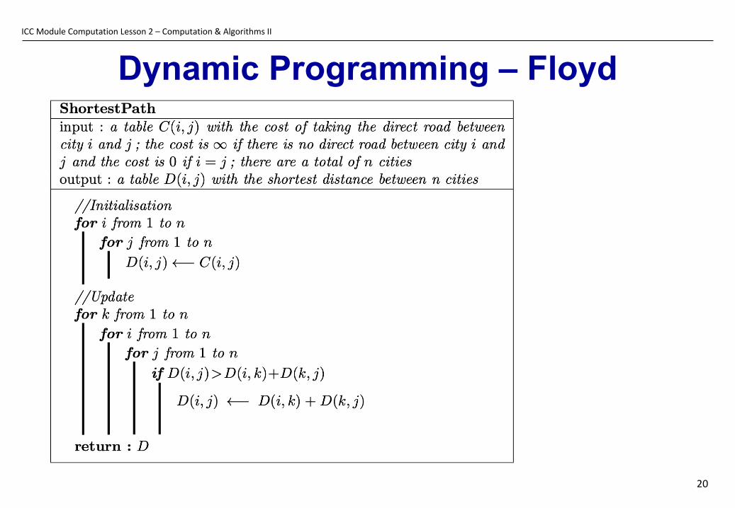
Dynamic Programming – Floyd


21

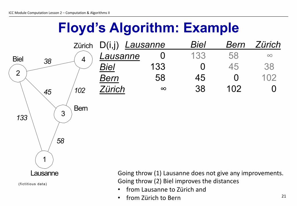
Floyd’s Algorithm: ExampleLausanne Biel Bern Zürich

0 133 58 ∞133 0 45 3858 45 0 102∞ 38 102 0

Zürich

3

1

Lausanne( f ic t i t ious data)

4

Bern

102

58

45

38

133

Biel

2

D(i,j)LausanneBielBernZürich

Going throw (1) Lausanne does not give any improvements.Going throw (2) Biel improves the distances • from Lausanne to Zürich and• from Zürich to Bern


22

Floyd’s Algorithm: Example

D0 = D 1

Lausanne Biel Bern Zürich0 133 58 ∞

133 0 45 3858 45 0 102∞ 38 102 0

D2 =

Zürich

3

1


4

Bern

102

58

45

38

133Lausanne Biel Bern Zürich

0133 0 58 45 0

171 38 83 0

Going throw (1) Lausanne does not give any improvements.Going throw (2) Biel improves the distances • from Lausanne to Zürich and• from Zürich to Bern

Biel

2


23

Lausanne Biel Bern Zürich0

133 0 58 45 0

171 38 83 0

Floyd’s Algorithm: Example

D3 =

Zürich

3

1


4

Bern

102

58

45

38

133Lausanne Biel Bern Zürich

0103 0 58 45 0

141 38 83 0

Going throw (3) Bern improves the distances • from Lausanne to Biel and• from Zürich to LausanneGoing throw (4) Zürich does not give any improvements

Biel

2 D2 =

Note: it also works for asymmetric graphs (directed graphs)

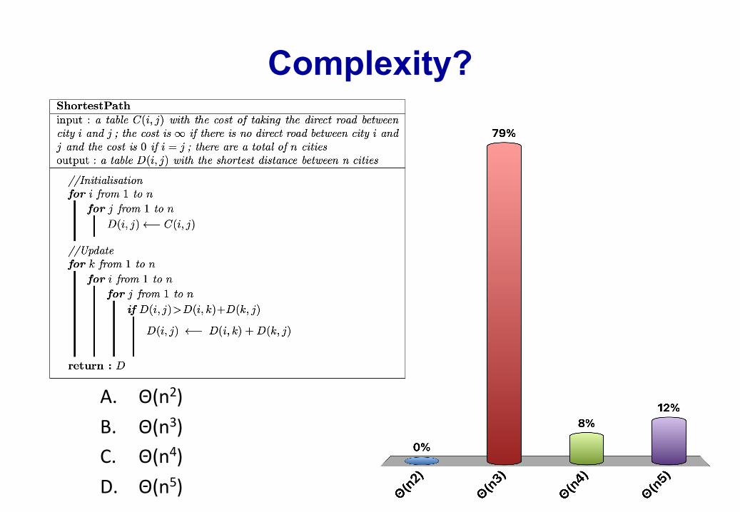
Complexity?

A. Θ(n2)B. Θ(n3)C. Θ(n4)D. Θ(n5)


25

§ There is no miracle recipe to find an algorithm, but there exist big families of resolution strategies:• decompose (e.g., “recursion”): try to solve the

problem by decomposing it in simpler (or smaller) instances

• decompose and regroup (e.g., “dynamic programming”): memorize intermediate computations to avoid executing them several times

Conclusion


26

Questions ?


27

§ About 300 copies sorted by SCIPER number§ How many copies do you have to look at (in the

worst case) in order to find your copy?

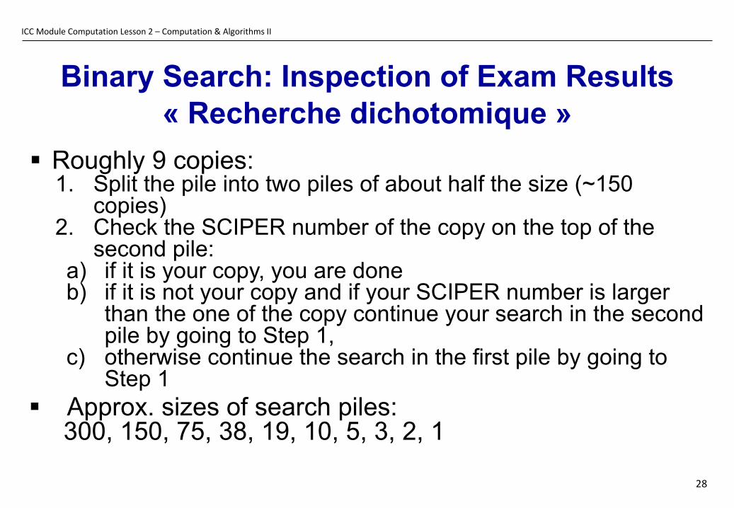
Binary Search: Inspection of Exam Results« Recherche dichotomique »


28

§ Roughly 9 copies:1. Split the pile into two piles of about half the size (~150

copies)2. Check the SCIPER number of the copy on the top of the

second pile:a) if it is your copy, you are doneb) if it is not your copy and if your SCIPER number is larger

than the one of the copy continue your search in the second pile by going to Step 1,

c) otherwise continue the search in the first pile by going to Step 1

§ Approx. sizes of search piles: 300, 150, 75, 38, 19, 10, 5, 3, 2, 1

Binary Search: Inspection of Exam Results« Recherche dichotomique »

information, computation, and communication

Documents