INFORMATION CASCADES IN THE LABORATORY

Lisa R. Anderson and Charles A. Holt*

AbstractWhen a series of individuals with private information announce public predictions, initial

conformity can create an “information cascade” in which later predictions match the earlyannouncements. This paper reports an experiment in which private signals are draws from anunobserved urn. Subjects make predictions in sequence and are paid if they correctly guesswhich of two urns was used for the draws. If initial decisions coincide, then it is rational forsubsequent decision makers to follow the established pattern, regardless of their privateinformation. Rational cascades formed in most periods in which such an imbalance occurred.

In many economic situations, agents observe private signals of some underlying state and

make public decisions. Subsequent decision makers face a dilemma if their own private signal

is indicative of a state that is unlikely given the previously observed decisions. An “information

cascade” occurs when initial decisions coincide in a way that it is optimal for each of the

subsequent individuals to ignore their private signals and follow the established pattern. For

example, suppose that a worker is not hired by several potential employers because of poor

interview performances. Knowing this, an employer approached subsequently may not hire the

worker even if the employer’s own assessment is favorable, since this information may be

dominated by the unfavorable signals inferred from previous rejections.1 Sushil Bikhchandani,

David Hirshleifer, and Ivo Welch (1992) discuss other examples and some simple models of the

cascade process. They point out that the conformity of followers in a cascade contains no

informational value, and in this sense, the cascade is fragile and can be upset by the arrival of

new public information.

* Lisa R. Anderson is Assistant Professor of Economics at American University, Washington, D.C. Charles A. Holtis Professor of Economics at the University of Virginia, Charlottesville, VA. This research was supported in part bygrants from the University of Virginia Bankard Fund and the National Science Foundation (SES90-12694 and SES93-20617). We wish to thank (without implicating) Michael Baye, Laura Clauser, Doug Davis, Dan Levin, Kevin McCabe,Roger Sherman, Steve Stern, Chris Swann, Robert Tollison, Darla Young, Nat Wilcox, and Marc Willinger forsuggestions.

1 Steve Stern (1990) presents an econometric study based on a model in which a longer duration of job search isinterpreted by employers as evidence that a worker has low skills.

As indicated above, an information cascade can result from rational inferences that others’

decisions are based on information that dominates one’s own signal. Particularly interesting is

the possibility of a reverse cascade; the initial decision makers are unfortunate to observe private

signals that indicate the incorrect state, and a large number of followers may join the resulting

pattern of “mistakes”, despite the fact that their private signals are more likely to indicate the

correct state.2 Even a qualified worker will sometimes make a bad impression in an interview,

and a series of rejections can create a reverse cascade that eliminates many future job

opportunities.3 Cascade-like behavior might also arise in financial markets, where trading

decisions come across a ticker tape in sequence. Even if early traders have no inside

information, others may incorrectly infer that the previous trades reveal private information.

These followers may then trade in a manner that suggests inside information, drawing in others.

In this way, some randomness in initial trades might create a price movement that is not

supported by fundamentals, as in a reverse cascade. Colin Camerer and Keith Weigelt (1991)

report some trading sequences in laboratory experiments that seem to fit this pattern.

There are several reasons to doubt that cascades develop in this way. First, human

subjects frequently deviate from rational Bayesian inferences in controlled experiments, especially

when simple rule-of-thumb heuristics are available.4 Second, with sequential announcements,

decision makers must make inferences about others’ rationality. Third, much of the evidence

offered in support of the rational view of cascades consists of anecdotes about patterns in fashion,

papers getting rejected by a sequence of journals, the risk of entering the academic job market

too early, etc. Laboratory experiments can provide more decisive evidence on the validity of the

rational view of cascades.

Several alternatives to the Bayesian view of conformity have been suggested.

Psychologists and decision theorists have found a tendency for subjects to prefer an alternative

that maintains the “status quo”. For example, William Samuelson and Richard Zeckhauser

2 Cf. John Dryden: “Nor is the people’s judgement always true; the most may err as grossly as the few.”

3 Other examples and applications are discussed in A. V. Bannerjee (1992) and Welch (1992).

4 See Daniel Kahneman and Amos Tversky (1973) and David Grether (1980 and 1992). Camerer (1995) and DougDavis and Charles Holt (1993, chapter 8) review this literature and provide additional references.

2

(1988) gave subjects hypothetical problems with several alternative decisions. When one of the

alternatives was distinguished as being the status quo, it was generally chosen more often than

when no alternative was distinguished.5 This systematic preference for the status quo is an

irrational bias if the decision maker’s private information is at least as good as the information

available to the people who established the status quo. In answering a question about an

unfamiliar decision problem, however, it can be rational for a subject to select the status quo

option if it is reasonable to believe that this status quo was initially established on the basis of

good information or bad experiences with alternatives. Even in non-hypothetical decision-making

situations, it may be very difficult for a researcher to infer what people think about the quality

of others’ sources of information. It is possible to control information flows in the laboratory

by drawing balls from urns, and therefore, to determine whether subjects tend to follow previous

decision(s) only when it is rational.

Another non-Bayesian explanation of patterns of conformity is that people derive utility

from herding together or that they are averse to the risk of standing alone.6 For example, a

forecaster may prefer the chance of being wrong with everybody else to the risk of providing a

deviant forecast that turns out to be the only incorrect guess.7 These other interpersonal factors

can be minimized in a laboratory experiment with anonymity and careful isolation of subjects.8

5 The status-quo version of question 2 from Samuelson and Zeckhauser (1988, pp. 52-53) is: “You are a seriousreader of the financial pages but until recently have had few funds to invest. That is when you inherited a portfolio ofcash and securities from your great uncle. A significant portion of this portfolio is invested in moderate-risk CompanyA. You are deliberating whether to leave the portfolio intact or to change it by investing in other securities. (The taxand broker commission consequences of any change are insignificant.) Your choices are (check one): ____ a) Retainthe investment in moderate-risk Company A. Over a year’s time, the stock has a .5 chance of increasing 30% in value,a .2 chance of being unchanged, and a .3 chance of declining 20% in value. ____ b) Invest in high-risk Company B.Over a year’s time, the stock has a .4 chance of doubling in value, a .3 chance of being unchanged, and a .3 chance ofdeclining 40% in value. ____ c) Invest in treasury bills. Over a year’s time, they will yield a nearly certain return of9%. ____ d) Invest in municipal bonds. Over a year’s time, these will yield atax-freerate of return of 6%.”

6 “To do exactly as your neighborsdo is the only sensible rule....” (Emily Post, 1922, chapter 33).

7 John Maynard Keynes (1965, p.158) notes that “Worldly wisdom teaches that it is better for reputation to failconventionally than to succeed unconventionally.”

8 Cascade-like behavior is sometimes observed in asset market experiments in which some investors are informedabout a state of nature and others are not (Charles Plott and Shyam Sunder, 1982). In these markets, the uninformed tendto follow the trading patterns of the insiders well enough to minimize earnings differences between the two groups.

3

This paper reports a cascade experiment that is based on a specific parametric model taken from

Bikhchandani, Hirshleifer, and Welch (1992). This model is outlined in section I. Section II

describes the experimental procedures, and sections III, IV, and V contain an analysis of the

results. The final section contains a conclusion.

I. A SYMMETRIC MODEL

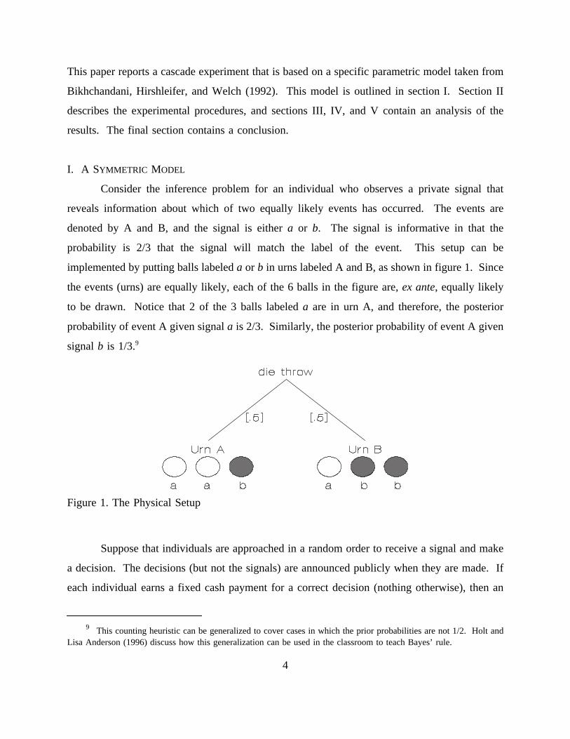
Consider the inference problem for an individual who observes a private signal that

reveals information about which of two equally likely events has occurred. The events are

denoted by A and B, and the signal is eithera or b. The signal is informative in that the

probability is 2/3 that the signal will match the label of the event. This setup can be

implemented by putting balls labeleda or b in urns labeled A and B, as shown in figure 1. Since

the events (urns) are equally likely, each of the 6 balls in the figure are,ex ante, equally likely

to be drawn. Notice that 2 of the 3 balls labeleda are in urn A, and therefore, the posterior

probability of event A given signala is 2/3. Similarly, the posterior probability of event A given

signalb is 1/3.9

Suppose that individuals are approached in a random order to receive a signal and make

Figure 1. The Physical Setup

a decision. The decisions (but not the signals) are announced publicly when they are made. If

each individual earns a fixed cash payment for a correct decision (nothing otherwise), then an

9 This counting heuristic can be generalized to cover cases in which the prior probabilities are not 1/2. Holt andLisa Anderson (1996) discuss how this generalization can be used in the classroom to teach Bayes’ rule.

4

expected-utility maximizer will always choose the urn with the higher posterior probability. The

first decision maker in the sequence, whose only information is the private draw, will predict

event A if the signal isa and will predict event B if the signal isb. Hence, the prediction made

by the first person will reveal that person’s private draw.

If the second person’s draw matches the label of the first person’s prediction, then the

second person should also follow the first person’s prediction. But suppose that the first person

predicts A and the second person drawsb. The second person should infer that the first draw

wasa. This inference, combined with theb signal, results in posterior probabilities of 1/2 since

the priors are 1/2 and the sample is balanced. In our initial discussion, we assume that the

second person will choose the event that matches the label of the private draw when this label

differs from the first decision.10 This assumption is reasonable when there is a positive

probability that the first person makes an error (e.g., drawsa and predicts B). This assumption

is also supported by an econometric analysis of the error rates to be reported below.

Suppose that each subsequent individual assumes that others use Bayes’ rule to make

predictions. For example, if the first two decisions are A and the third person observes ab

signal, then this person is responding to an inferred sample ofa on the first two draws, andb on

the third draw. Since the events are equally likelya priori, and since the sample favors event

A, the posterior probability of A is greater than 1/2. In this case, the third person should predict

event A in spite of the privateb signal. Hence, the first two decisions can start a cascade in

which the third and subsequent decision makers ignore their own private information. Whenever

the first and second individuals make the same prediction, all subsequent decision makers should

follow, regardless of their own private information. A cascade can also form, for example, if the

first two decisions differ and the next two match. In all cases, it takes an imbalance of two

decisions in one direction to overpower the informational content of subsequent individual

signals.

If individuals recognize that decisions made after the beginning of a cascade are not

informative, they will ignore these “irrelevant” decisions in their probability assessments. But

10 When the posterior probabilities are 1/2, we could make an alternative assumption that the decision is random,i.e., that it matches the label of the private signal with probability 1/2. This would not alter the analysis of cascadeformation that follows, but it would alter some of the numerical probability calculations, as indicated in the next footnote.

5

if someone breaks out of a cascade pattern and predicts the other event, then it is reasonable to

Table I. Posterior Probability of Event A

number ofasignals

number ofb signals

0 1 2 3

0 1/2 1/3 1/5 1/9

1 2/3 1/2 1/3 1/5

2 4/5 2/3 1/2 1/3

3 8/9 4/5 2/3 1/2

assume that this deviant decision reveals a private signal that is contrary to the cascade, because

the expected cost of deviating would be higher if the signal matched those inferred from previous

decisions.11 Therefore relevant signals are those inferred from decisions made before a cascade

starts, from the two decisions that start a cascade, and from non-Bayesian deviations from a

cascade. Letn be the number of relevanta signals and letm be the number of relevantb signals.

Then Bayes’ rule can be used to calculate the posterior probability of event A, given any

sequence of sample draws:

11 Of course, even the “irrelevant” decisions of followers in a cascade will convey some information in a modelwith the possibility of decision error, so the probability calculations in this section should be interpreted as appropriatein the limit as errors are reduced to zero. The econometric analysis of errors in section IV explicitly incorporates therelationship between the expected costs of each type of error and the resulting informational content of the error.

6

Table 1 can be used to determine the posterior probability of event A for any combination of

(1)

Pr(A|n, m) Pr(n,m|A)Pr(A)Pr(n,m|A)Pr(A) Pr(n,m|B)Pr(B)

(2/3)n(1/3)m(1/2)

(2/3)n(1/3)m(1/2) (1/3)n(2/3)m(1/2)

2n

2n 2m.

draws. Notice that when the signals are balanced, the posterior equals the prior of 1/2; it is the

difference in the number ofa andb signals that determines the posterior. In this manner, Bayes’

rule corresponds to a simple counting heuristic. Section VI reports results with an asymmetric

design in which Bayes’ rule and counting can give different predictions.

II. PROCEDURES

The 72 subjects in this experiment were recruited from undergraduate economics courses

at the University of Virginia and had no previous experience with this experiment. A $5

participation fee was paid upon arrival, and subsequent earnings, which averaged about $20, were

paid privately in cash when the subjects were released. In each session, six subjects were

decision makers and one was randomly chosen to serve as a “monitor” to assist the experimenters

with rolling dice and drawing marbles. The instructions in the Appendix were read aloud to

participants, and the monitor was asked to ensure that the procedures in the instructions were

followed. Then subjects were taken to their seats, which were separated by large foam board

partitions.12

A session consisted of 15 periods and lasted for about one and a half hours. At the start

of each period, the monitor threw a die to determine which of two urns would be used for the

period. As shown in figure 1, urn A contained twoa balls and oneb ball, and urn B contained

12 These partitions extended three feet beyond the desk on each side, and effectively isolated the subjects. Theroom has three rows of desks and one subject was seated at either end of each row, so subjects were at least 10 feet apart.The monitor was isolated behind a partition at the front of the room, making it impossible for participants to see eitherthe throw of the die that determined the urn or the private draws of other subjects.

7

two b balls and onea ball.13 The experimenters took great care to assure that all marbles were

uniform in size, color, and weight. The “urns” were envelopes marked A and B containing the

appropriate marbles. Urn A was used if the throw of the die was one, two, or three; urn B was

used otherwise. Once the urn was selected, the contents were emptied into an unmarked

container. Unintended visual clues were prevented by using the same container, regardless of

the urn used.

In each period, subjects were chosen in a random order and were approached by an

experimenter to see one private draw from the container, with replacement. After seeing a

private draw, the subject would record it and write the urn decision, A or B, on a record sheet.

The experimenter reported the decision to an announcer, who did not know either the urn in use

or the subject’s private draw.14 When the decision was announced, other subjects recorded this

decision on their record sheets. In this way, each subject knew his or her own private draw and

the prior decisions of others, if any, before making a prediction. This process continued until

all subjects had made decisions. Then the monitor announced which urn had been used, and

subjects recorded their earnings: $2 for a correct prediction and nothing otherwise. The session

was terminated after 15 periods.15,16 Three sessions followed this procedure, and three other

13 Thea balls were actually light marbles and theb balls were actually dark marbles. The draws were referred toas light and dark. In our discussion of the results, it is convenient to have the labels of the balls indicate the more likelyurn, but this would have been too suggestive for the actual experiment.

14 In an admittedly uncontrolled demonstration experiment in an experimental economics class, students seemedto use visual and voice cues in an attempt to discern whether the person making a prediction was agonizing over a sampledraw that seemed unlikely given the pattern of earlier public predictions. In fact, a reverse cascade was broken in thismanner.

15 Several practice periods were conducted at the beginning of each session to familiarize the subjects with theprocedures; we continued with practice periods until each urn had been selected at least once. In the practice periods,the subjects observed as the monitor threw the dice and emptied the contents of the appropriate urn into the container.Draws from the container were not private in the practice session and subjects were not asked to make decisions,precluding any reputation effects. This public demonstration of the mechanics of the drawing process was added aftera pilot session in which one of the subjects made a pattern of mistakes that suggested misunderstanding or distrust.Cascades were nevertheless observed in the pilot, but it is not included since it had a slightly different structure from thesessions reported here.

16 At the conclusion of the first session, subjects were asked if there was any confusion or bias in procedures andif they had suggestions for improving the experiment. None of the subjects reported any difficulty understanding theinstructions or the procedures. The only suggested improvement in the instructions was to eliminate some of the repetitionin the oral instructions across periods.

8

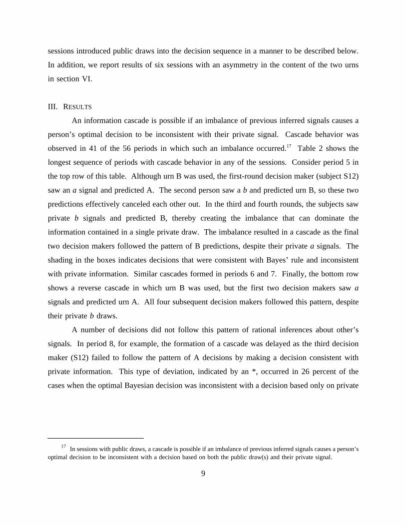
sessions introduced public draws into the decision sequence in a manner to be described below.

In addition, we report results of six sessions with an asymmetry in the content of the two urns

in section VI.

III. RESULTS

An information cascade is possible if an imbalance of previous inferred signals causes a

person’s optimal decision to be inconsistent with their private signal. Cascade behavior was

observed in 41 of the 56 periods in which such an imbalance occurred.17 Table 2 shows the

longest sequence of periods with cascade behavior in any of the sessions. Consider period 5 in

the top row of this table. Although urn B was used, the first-round decision maker (subject S12)

saw ana signal and predicted A. The second person saw ab and predicted urn B, so these two

predictions effectively canceled each other out. In the third and fourth rounds, the subjects saw

private b signals and predicted B, thereby creating the imbalance that can dominate the

information contained in a single private draw. The imbalance resulted in a cascade as the final

two decision makers followed the pattern of B predictions, despite their privatea signals. The

shading in the boxes indicates decisions that were consistent with Bayes’ rule and inconsistent

with private information. Similar cascades formed in periods 6 and 7. Finally, the bottom row

shows a reverse cascade in which urn B was used, but the first two decision makers sawa

signals and predicted urn A. All four subsequent decision makers followed this pattern, despite

their privateb draws.

A number of decisions did not follow this pattern of rational inferences about other’s

signals. In period 8, for example, the formation of a cascade was delayed as the third decision

maker (S12) failed to follow the pattern of A decisions by making a decision consistent with

private information. This type of deviation, indicated by an *, occurred in 26 percent of the

cases when the optimal Bayesian decision was inconsistent with a decision based only on private

17 In sessions with public draws, a cascade is possible if an imbalance of previous inferred signals causes a person’soptimal decision to be inconsistent with a decision based on both the public draw(s) and their private signal.

9

information. Over all six sessions, about 4 percent of the decisions were inconsistent with both

Bayes’ rule and private information.18

Table 2. Data for Selected Periods of Session 2

Period Urn

Used

Subject Number: Urn Decision

(private draw) Cascade

Outcome1st

round

2nd

round

3rd

round

4th

round

5th

round

6th

round

5 B S12: A

(a)

S11: B

(b)

S9: B

(b)

S7: B

(b)

S8: B

(a)

S10: B

(a)

cascade

6 A S12: A

(a)

S8: A

(a)

S9: A

(b)

S11: A

(b)

S10: A

(a)

S7: A

(a)

cascade

7 B S8: B

(b)

S7: A

(a)

S10: B

(b)

S11: B

(b)

S12: B

(b)

S9: B

(a)

cascade

8 A S8: A

(a)

S9: A

(a)

S12: B*

(b)

S10: A

(a)

S11: A

(b)

S7: A

(a)

cascade

9 B S11: A

(a)

S12: A

(a)

S8: A

(b)

S9: A

(b)

S7: A

(b)

S10: A

(b)

reverse

cascade

Key: Shading -- Bayesian decision, inconsistent with private information.

* -- Decision based on private information, inconsistent with Bayesian updating. One question of

interest is the extent to which errors cause actual earnings to be lower than the earnings that

would result from Bayesian decisions in a theoretical model with no errors. TheBayes

distributionfor subject Si in a particular round is defined to be the Bayesian posterior distribution

on the urn used, assuming that others are Bayesians and that an obvious deviation from a

Bayesian decision by someone else reveals that person’s private information. For example,

18 A complete data appendix is available from the authors on request.

10

consider the Bayesian calculations for the top row of table 2. Subject S12 drew ana in the first

round, so the Bayes distribution at this point was 2/3 for A. After split decisions of A and B in

the first 2 rounds of this period, the Bayes distribution for S9 with ab signal in the third round

was 2/3 for urn B. Expected-utility-maximizing decisions based on the Bayes distribution will

be calledoptimal. The optimal decision is A if and only if the Bayesian posterior for urn A is

greater than or equal to 1/2. As noted above, the shading in the table indicates rounds in which

the decision was optimal but inconsistent with private information.

We will use expected payoff calculations to measure both the extent to which subjects do

worse than choosing optimally and the extent to which they do better than just choosing

randomly. The expected payoff for a particular decision depends on the information used to

make decisions, and all expected payoffs are calculated on the basis of the Bayes distributionat

the time the decision was made. The optimal expected payoffis the expected earnings for a

person who makes an optimal urn decision at each stage using the appropriate Bayes distribution.

The random-choice expected payoffis the expected earnings for a person who makes decisions

randomly in each period. Theprivate-information expected payoffis the expected earnings for

a person who makes a decision only on the basis of the private draw. Finally, theactual

expected payoffis the expected earnings for the person’s actual decision. The sums of the

expected payoffs for all 15 periods will be denoted byπO, πR, πP, and πA for the optimal,

random-choice, private-information, and actual expected payoffs respectively.

These expected payoffs are used to construct measures of how efficiently people use

relevant information to make decisions. We will normalize the efficiency measure so that

optimal decisions are 100 percent efficient and random choices are 0 percent efficient:

Theactual efficiencyis the difference between the actual expected payoff and the random-choice

actual efficiency100(π A π R)

(π O π R).

payoff expressed as a percentage of the difference between the optimal expected payoff and the

random-choice payoff.19 As a benchmark, we also calculate theprivate information efficiency

19 Even a random chooser may get a measure above zero if they are lucky in their choices.

11

as the difference between the private-information expected payoff and the random-choice payoff

expressed as a percentage of the difference between the optimal expected payoff and the random-

choice payoff:private information efficiency

100(π P π R)

(π O π R).

This measure is also between 0 and 100 and is useful as a basis of comparison with actual

efficiency, to determine the extent to which a person used information inferred from public

decisions.

Actual efficiency, averaged over all subjects in the symmetric design being discussed here,

was 91.4 percent, and private-information efficiency was 72.1 percent. Of the 36 subjects, about

two-thirds (22) obtained actual efficiencies of 100 percent, indicating perfect conformity with

Bayes’ rule.20 About two-thirds of the others (9 of 14) also did better than they would have

with decisions based solely on private information. Several subjects seemed to disregard the

information in others’ previous predictions, which is a plausible reaction to the possibility that

others are making errors. The next section uses a logit model to analyze the effects of decision

errors, caused by independent additive shocks, on posterior probabilities.

IV. A N ECONOMETRIC ANALYSIS OF ERRORS21

This section presents a dynamic model in which people calculate posteriors allowing for

the possibility of errors in earlier decisions. Error rates are econometrically estimated assuming

a logistic distribution of independent shocks to expected payoffs. The first step in the analysis

is the calculation of expected payoffs. Suppose that the first person in the sequence sees a draw

of a, and therefore has a posterior of 2/3 for urn A and 1/3 for urn B. The expected payoff for

choosing A is 2/3 times the reward of $2 for a correct prediction, and the expected payoff for

choosing B is 1/3 times $2. Let these expected payoffs be denoted byπA andπB respectively,

and let the probability that the decision maker in round i chooses urn A be denoted by Pr(Di =

20 However, four of these subjects also had a private information efficiency of 100; these people faced a series ofchoices in which relying only on private information resulted in the optimal decisions.

21 This section summarizes the econometric analysis in Chapter 7 of Anderson’s (1994) doctoral dissertation.

12

A). Then the logit model specifies that this probability is an increasing exponential function of

πA:

Pr(Di A) eβπ A

eβπ A

eβπ B

1

1 e β (π A π B).

Thus the probability of choosing urn A is an increasing function of the payoff difference,πA -

πB, whereβ parameterizes the sensitivity to payoff differences.22 The tendency to make errors

diminishes as ß→ ∞, and the probability of making the decision with the highest payoff goes to

1. Conversely, behavior becomes essentially random as ß→ 0, in which case the decision

probabilities approach 1/2, regardless of expected payoffs. When the expected payoffs are equal,

the logit function specifies a probability of 1/2 for each decision.

The inference problem becomes more interesting for the decision maker in round 2 if the

second person in the sequence knows that the first one may make an error. When such errors

are possible, the private draw seen by the second person contains more information than can be

inferred from the first person’s decision. The estimated value of ß for the first round can be used

to determine the decision probabilities: Pr(D1 = A| s1 = a), Pr(D1 = A| s1 = b), etc., where s1 is

the signal seen by the first round decision maker. These probabilities, together with Bayes’ rule,

can be used to calculate the posterior probabilities for the second person conditional on D1 and

on the second person’s signal: Pr( Urn = A| D1, s2).23 This posterior determines the second

person’s expected payoff for each prediction. Since the second person may also make an error,

we assume that this person’s expected payoffs for each prediction determine decision probabilities

via the logit choice function given above.

22 The functional form of the logit model can be derived by assuming that there is an independent random shockto each of the expected payoffs, and that these shocks have a logistic distribution.

23 There are 22 (= 4) possible combinations of information that a second round decision maker might use tocalculate posteriors. These calculations are increasingly tedious for later decision making rounds because of theincorporation of all previous information. For a sixth round decision maker there are 26 (= 64) possible combinations ofprevious decisions and private signals that this person might observe. Posteriors for each round depend on the errordistributions for all previous rounds, making the calculation more complicated. These calculations can be found in Chapter6 of Anderson (1994).

13

Table 3. Econometric Results by Round

Round 1 2 3 4 5 6

β 2.84 8.67 4.95 2.94 3.03 4.29

(standard error) (0.36) (2.03) (1.02) (0.64) (0.58) (1.15)

number of errors 4 3 6 14 13 7

Notice that the error structure is recursive; theβ parameter for the first person in the

sequence affects the second person’s expected payoffs, which are used in turn to estimate aβ

parameter for the second stage decision. In each round, theβ estimates for previous rounds are

used to calculate the expected payoffs for each decision (urn A or urn B), conditional on each

possible combination of the current draw (a or b) and the decisions observed in previous rounds.

Then the difference in expected payoffs for a round constitutes the independent variable in the

estimation for that round. Table 3 reports the results of this recursive estimation, using a

maximum likelihood routine in GAUSS.24 The model predicts correctly in 493 out of 540

cases. This econometric approach changes the error classification of about 5 percent of the

individual decisions, as compared with the previous section’s analysis that assumed no error. The

inclusion of errors in the expected payoff calculation does not change the cascade outcome

classification for any period.

Notice from the round 1 column of the table that there were even some errors in the first

round, where the optimal prediction is clearly to reveal one’s own draw. Thus the first-round

prediction is a noisy signal of the first-round draw, and therefore, the second person in the

sequence should not be indifferent when the draw observed in the second round is inconsistent

with the first-round prediction. In such cases, the parameter estimate from the first column in

table 3 can be used to predict that the second person will make a decision consistent with his/her

private draw with a probability of 0.96. In fact, the second person did make a prediction that

24 The estimation used the Newton-Raphson algorithm to minimize the negative of the log likelihood function. Analternative to the recursive method is to constrainβ to be the same for all rounds, which resulted in aβ of 3.78.However, the recursive method reported in table 3 provides a better fit based on a likelihood ratio test.

14

matched the private draw in 95 percent of the cases in which there was a conflict between the

first-round prediction and the second-round draw.

The logit analysis shows how a cascade can result from rational behavior, even in the

presence of decision error. If the first two people predict A and the third person sees ab draw,

the parameter estimates in table 3 can be used to show that the third person should still start the

cascade, since the posterior for urn A (given two A decision and ab draw) is 0.5745.25 Since

the posterior for urn A is higher than the posterior for urn B, the expected payoff for predicting

A is higher. Hence the logit probability for decision A is greater than 1/2.

Similarly, the logit analysis of decision errors provides a natural framework in which to

interpret irrational deviations from a cascade pattern. For example, suppose that someone

announces a B decision that differs from a cascade pattern of A decisions. If the deviator saw

an a draw, then the deviation is a more costly error than if the deviator saw ab draw. For this

reason, a deviation from a cascade of A decisions should be interpreted as evidence that the

deviator was more likely to have seen ab signal. In fact, 15 of the 16 deviations from cascade

patterns were made after seeing a private draw that favored the urn that was not predicted by

previous decision makers. The information inherent in whether or not someone deviates from

a cascade is incorporated into the posteriors that are based on the application of Bayes’ rule in

a probabilistic choice context.26 Suppose that a person sees ana draw. The estimates in table

3 can be used to calculate a posterior for urn A of 0.84 if the person sees two previous A

decisions and no B decisions, and this posterior is only marginally higher (0.85) if the person

sees three previous A decision. But if the fourth decision maker sees two A decisions and a

(third) B decision, prior to thea draw, then the posterior for urn A falls to 0.73. Thus the

deviation from the cascade pattern lowers the probability of urn A by much more than it is

increased by the continuation of the cascade pattern.

To summarize, many of the interesting patterns of behavior can be explained when the

analysis is modified to include the possibility that others make errors. This model explains why

25 These calculations are provided in Anderson (1994).

26 The calculations are straightforward but tedious. See Anderson (1994) for details.

15

a second-round decision makers almost always makes a prediction consistent with private

information, even when this prediction differs from that made in the first round. Most

importantly, the error estimates are small enough so that it is still optimal to follow a cascade

once it develops even if one’s private information indicates otherwise. The information inferred

from others’ decisions depends on the context in which they are made. In most cases, the

possibility of error makes others’ decisions less informative. However, when errors by others

cause them to break out of a cascade pattern, their decisions are almost always indicative of their

private signal, thus providing much information for those later in the decision sequence. In

addition to the random errors discussed above, some subjects make systematic deviations from

Bayesian decision making. These errors can often be linked to one of biases which is discussed

in the next section.

V. BIASES

Unlike the random errors discussed in the previous section, many of the information

processing biases of interest to psychologists are systematic in nature. These biases are more

likely to show up in environments that are richer than the highly controlled ball-and-urn setting

discussed here. Nevertheless, even in this environment, it is possible to identify some patterns

of behavior that would be implied by previous research on biases. For simplicity, the posteriors

reported in this section are calculated without random decision error and the focus is on other

(non-random) biases that might be present.

A. Status Quo and Representativeness Bias

Recall that a cascade is a situation where it isrational for subjects to follow thestatus

quo. The high actual efficiencies indicate that most subjects followed others when it was rational

to do so, and not otherwise. If there is an additional preference to go along with the crowd, then

this status quobias should show up most clearly when the Bayes distribution for A is close to

1/2. Posteriors of 1/2 are most common in the second round, i.e. when the second decision

maker’s signal differs from the signal inferred from the first-round decision. We think that it is

reasonable to identify the previous decision as being the status quo, even when there is only one

16

previous decision.27 Over all 6 sessions with the symmetric design, there were 68 instances in

which the Bayes distribution was 1/2 and the private information did not match the label of the

previous decision. In 57 of these 68 cases, the subject did not follow the previous decision, but

rather made decisions that were consistent with their private information. If there is a systematic

bias in favor of following the previous decision(s), it is too weak to show up in these data.28

Another type of bias in decision making that has been suggested is that subjects tend to

underweight prior probabilities and focus on the similarity of their sample to a particular

population (Kahneman and Tversky, 1973). This notion of similarity or “representativeness” is

easiest to explain in the context of drawing balls from urns (Grether, 1980 and 1992). A sample

of draws is said to be representative of an urn if the sample proportions match those of the urn.

For example, a sample of twoa signals and oneb signal is representative of urn A in figure 1.29

By adding two public draws after the fourth round in sessions 4 and 5, we provided the fifth and

sixth decision makers with samples of three draws, making representativeness possible. Before

seeing the two public draws and their own private draw, these decision makers had priors based

on the previous decisions of others. They then formed their posteriors using the three additional

draws. The combination of the two public draws and the private draw matched the contents of

one urn in thirty-six cases. In ten of these cases, the Bayesian posterior for the urn that the

27 After all, many of the hypothetical questions used in the original Samuelson and Zeckhauser (1988) studyexplained the status quo to the subjects as being determined by a previous decision, e.g., the investment decision of arecently deceased great uncle. One version of the investment question (2) was phrased so that the subject was told howthe money was invested previously, and another version was phrased identically except that no information was givenabout how the money was previously invested. Although the same investment options were used in both versions, eachoption was selected more frequently if it was identified as the great uncle’s portfolio, i.e., the status quo.

28 These deviations from the status quo are consistent with an analysis that incorporates decision error. When othersmake errors, one’s own information becomes more informative. With errors incorporated in the calculations, all of theposterior probabilities in this section (with samples of A andb or B anda) change so that the urn represented by asubject’s private draw is slightly favored to the urn previously predicted.

29 Grether (1980) showed subjects samples from one of two possible urns, with the urn being selected with a knownprior probability. When individual subjects were asked which urn was being used, the frequency of Bayesian decisionswas clearly lower when the sample matched the contents of the urn with the lower posterior probability. By altering theprior probabilities, Grether was able to compare decisions made under identical posterior probabilities, but withrepresentativeness either reinforcing or contradicting the Bayesian decision. There were no public, sequential decisionsin the Grether experiment, so cascades were not possible.

17

sample “represented” was less than 1/2, and the subject made a decision consistent with Bayes’

rule in all ten cases.30 There is no support for representativeness in this context.31

B. Counting Heuristic

As discussed above, one implication of the symmetric composition of the two urns in

figure 1 is that the optimal Bayesian decision is to predict the urn that receives the greatest

number of observed and inferred signals, ignoring those that follow the formation of a cascade.

Therefore, we conducted six additional sessions with an asymmetric design in which counting

can be distinguished from Bayesian behavior.

Table 4. Physical Setup for the Asymmetric Design

Urn A

(used if the die is 1, 2, or 3)

Urn B

(used if the die is 4, 5, or 6)

6 a Balls

1 b Ball

5 a Balls

2 b Balls

In this asymmetric design, urns A and B are also equally likely to be chosen, but their

contents differ, as shown in table 4. As before, thea signal indicates that urn A is more likely,

and theb signal indicates that urn B is more likely. The asymmetry is that theb signal is much

more informative than thea signal, so that just counting the number of relevant decisions made

previously does not necessarily indicate a correct Bayesian decision.

30 Adding random decision error does not change the “correct” Bayesian prediction in any of these ten cases.

31 A possible explanation for the apparent lack of attention to representativeness is that priors in the cascadeexperiment are not in the form of instructions, as in Grether (1980 and 1992). Instead, priors in our setup are based onthe subjects’ own inferences about others’ signals.

18

Table 5 shows Bayesian posteriors for urn A (without decision error) as a function of the

Table 5. Posterior Probability of Event A for the Asymmetric Designa

number ofa signals

number ofb signals

0 1 2 3 4 5 6

0 0.50 0.33 0.20 0.11 0.06 0.03 0.02

1 0.55 0.38 0.23 0.13 0.07 0.04

2 0.59 0.42 0.27 0.15 0.08

3 0.63 0.46 0.30 0.18

4 0.68 0.51 0.34

5 0.71 0.55

6 0.75

a Shading indicates cases where Bayes’ rule and the counting rule make different predictions.

numbers ofa andb signals.32 The four shaded entries in this table correspond to cases in which

there are morea signals, but a smaller number of informativeb signals causes the Bayesian

posterior for urn A to be less than 0.5. The asymmetric design was chosen to yield a high

probability that the sample sequences will create this conflict (subject to a constraint of keeping

the design simple).33

Table 6 shows partial results for one of the six sessions conducted with this asymmetric

design. In period 2, the first three subjects sawa signals and correctly predicted urn A. The

posterior probabilities for urn A (from table 5) are shown in parentheses to the right of the letter

indicating the signal observed by the subject. The fourth decision maker in this period saw the

32 The econometric analysis in section IV was based on the symmetric experimental design. Random error rateswere not estimated for this asymmetric design. Hence, the Bayesian posteriors reported in this section do not includerandom decision error.

33 We also considered using the symmetric design in figure 1 but with unequal probabilities of selecting the twourns. This approach was not followed since, if a six-sided die is used to make the chances of one urn go from 1/2 to 2/3,then the posterior for the urn with the higher prior is always greater than or equal to 1/2 after only one draw.

19

more informativeb signal. Using a counting rule, this person would also predict urn A, with

Table 6. Data for Selected Periods of Session 10

PeriodUrnUsed

Subject Number: Urn Decision(private draw, Bayesian posterior)

CascadeOutcome

1stround

2ndround

3rdround

4thround

5thround

6thround

2 A S60: A(a, 0.55)

S59: A(a, 0.59)

S55: A(a, 0.63)

S58: B(b, 0.46)+

S56: B(b, 0.30)+

S57: B(a, 0.51)**

3 A S58: A(a, 0.55)

S55: A(a, 0.59)

S59: A(a, 0.63)

S60: A(b, 0.46)*

S56: A(a, 0.71)

S57: A(a, 0.71)

4 A S57: A(a, 0.55)

S58: B(a, 0.59)**

S59: B(a, 0.42)+

S55: B(a, 0.42)

S60: B(a, 0.42)

S56: B(a, 0.42)

reversecascade

5 B S58: B(b, 0.33)

S57: B(b, 0.20)

S59: B(a, 0.38)

S55: B(b, 0.20)

S56: B(a, 0.38)

S60: B(a, 0.38)

cascade

Key:Shading -- Bayesian decision, inconsistent with private information.

+ -- Bayesian decision, inconsistent with counting.* -- Decision based on counting, inconsistent with Bayesian updating.** -- Decision inconsistent with Bayes’ rule and counting.

three (inferred)a signals and only one (observed)b signal. However, because of the asymmetry

in the contents of the urns, the posterior for urn A is only 0.46, and this subject correctly

predicted urn B. The subject in the fifth round also made a correct Bayesian decision in a case

where counting would have yielded a different prediction. The + marks in the table indicate

Bayesian decisions that are inconsistent with counting. The last subject in period 2 made a

decision that was inconsistent with both Bayes’ rule and counting, as denoted by the ** notation

in the table. The third period begins in the same way as the previous period, however the fourth

subject in the sequence makes a decision that is inconsistent with Bayes’ rule but consistent with

counting. This type of error is denoted by a single asterisk in the table. The shading in period

4 shows a reverse cascade that was triggered by an error in the second round. Over all six

sessions with the asymmetric design, cascades formed in 46 out of the 66 periods where they

were possible, i.e. where an optimal Bayesian decision was inconsistent with a subjects private

information. The incidence of reverse cascades was higher in this asymmetric design (18 out of

46) than in the symmetric design (13 out of 41).

20

While cascades are still prevalent in this asymmetric design, the effect of counting is to

reduce the incidence of rational Bayesian cascades from about 73 percent to 70 percent. When

Bayes’ rule and counting make different predictions in the asymmetric design, people make a

correct (Bayesian) decision half of the time (41 out of 82 cases).34 When counting makes no

prediction (i.e. there are equal numbers of observed and inferred signals of each type) the

percentage of correct decisions increases to 66 percent, as would be expected. In total, 115 of

the 540 decisions were inconsistent with Bayes’ rule, and over a third of these can be explained

by counting.

Besides categorizing decisions, it is useful to calculate the expected gains and losses from

alternative decision rules. The previous efficiency calculations can be made with data from this

asymmetric design. Averaged over all subjects, actual and private information efficiencies were

67.6 percent and 45.2 percent, respectively. These are lower than the corresponding efficiencies

with the symmetric design where counting and Bayes’ rule always coincide. In addition to the

measures of actual and private information efficiency, we define counting efficiency to be the

percentage of the expected payoff gains for using a counting rule over random decision making:

whereπC is the expected payoff for making a decision based on counting. Twenty-one out of

counting efficiency100(π C π R)

(π O π R),

thirty-six subjects in the asymmetric design did better than counting in the sense that their actual

efficiencies exceeded counting efficiencies. Averaged over all subjects, however, counting

efficiency is approximately equal to actual efficiency. This is because the gains from Bayesian

decision making (instead of counting) were balanced by severe reductions in expected payoffs

when subjects made predictions that were inconsistent with both counting and Bayes’ rule.

VI. SUMMARY

Information cascades develop consistently in a laboratory situation in which other

incentives to go along with the crowd are minimized. Some decision sequences result in reverse

cascades, where initial misrepresentative signals start a chain of incorrect decisions that is not

34 A large fraction of these errors (29 out of 41) were made by a third of the subjects.

21

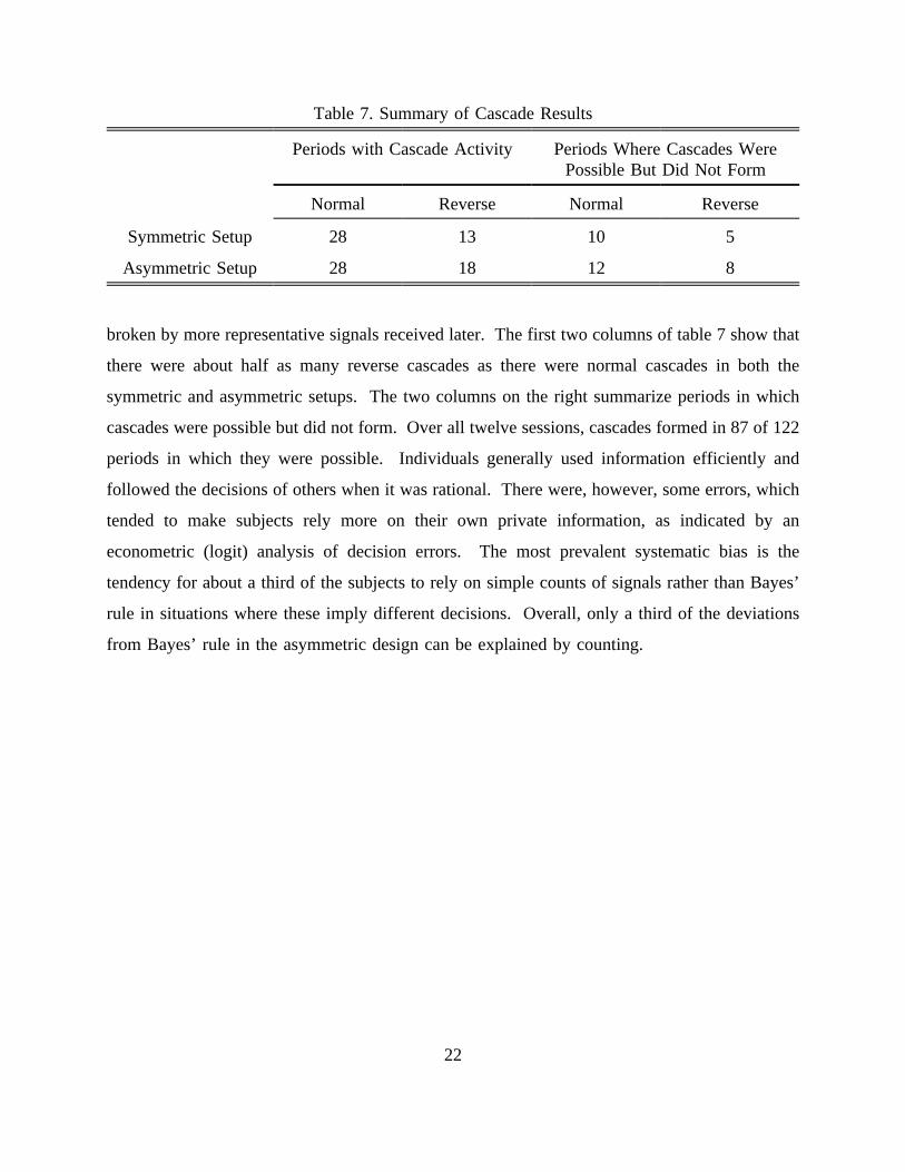
Table 7. Summary of Cascade Results

Periods with Cascade Activity Periods Where Cascades WerePossible But Did Not Form

Normal Reverse Normal Reverse

Symmetric Setup 28 13 10 5

Asymmetric Setup 28 18 12 8

broken by more representative signals received later. The first two columns of table 7 show that

there were about half as many reverse cascades as there were normal cascades in both the

symmetric and asymmetric setups. The two columns on the right summarize periods in which

cascades were possible but did not form. Over all twelve sessions, cascades formed in 87 of 122

periods in which they were possible. Individuals generally used information efficiently and

followed the decisions of others when it was rational. There were, however, some errors, which

tended to make subjects rely more on their own private information, as indicated by an

econometric (logit) analysis of decision errors. The most prevalent systematic bias is the

tendency for about a third of the subjects to rely on simple counts of signals rather than Bayes’

rule in situations where these imply different decisions. Overall, only a third of the deviations

from Bayes’ rule in the asymmetric design can be explained by counting.

22

APPENDIX: INSTRUCTIONS FORSYMMETRIC DESIGN

This is an experiment in the economics of decision making. Various agencies haveprovided funds for the experiment. Your earnings will depend partly on your decisions andpartly on chance. If you are careful and make good decisions, you may earn a considerableamount of money, which will be paid to you, privately, in cash, at the end of the experiment.At this time, we will give you $5. This payment is to compensate you for showing up today.

Before beginning, we will choose one of you to assist us in the experiment today. Thisperson, who will be called the monitor, will help us by throwing dice and drawing colored ballsfrom a container. The monitor will also observe procedures to insure that the instructions arefollowed. The monitor will be paid $15 at the end of the experiment in addition to the $5already paid. We will now assign each of you a number, and we will throw a multi-sided dieto select the monitor.

In this experiment, you will be asked to predict from which randomly chosen urn a ballwas drawn. We will begin by rolling a 6 sided die. If the roll of the die yields a 1, 2, or 3, wewill draw from urn A which contains 2 light balls and 1 dark ball. If the roll of the die yieldsa 4, 5, or 6, we will draw from urn B which contains 1 light ball and 2 dark balls. Therefore,it is equally likely that either urn will be selected.

Urn A

(used if the die is 1, 2, or 3)

Urn B

(used if the die is 4, 5, or 6)

2 Light Balls

1 Dark Ball

1 Light Ball

2 Dark Balls

Once an urn is determined by the roll of the die we will empty the contents of that urninto a container. (The container is always the same, regardless of which urn is being used.)Then we will come around to each of you and draw a ball from the container. The result of thisdraw will be your private information and should not be shared with other participants.Aftereach draw, we will return the ball to the container before making the next private draw. Eachperson will have one private draw, with the ball being replaced after each draw.

After each person has seen his or her own draw we will ask them to record the letter ofthe urn (A or B) that they think is more likely to have been used. When the first personapproached has indicated a letter, we will announce that letter. After announcing the firstperson’s decision, we will approach the second person and ask this person to record a letter (Aor B), which will then be announced. This process will be repeated until all remaining peoplehave made decisions. Finally, the monitor will inform everyone of the urn that was actuallyused. Everyone who correctly recorded the letter of the urn used earns $2. All others earnnothing.

The experiment will consist of 15 periods. The results for each period are recorded ona separate row on the decision sheet that follows. The period numbers are listed on the left sideof each row. Next to the period number is a blank that should be used to record the draw (Lightor Dark) that you see when we come to your desk. Write L (for Light) or D (for Dark) incolumn (0) at the time the draw is made. The columns numbered (1) through (6) should be usedto record the decisions as they are announced. When you are asked to record the letter of an urn,you will be able to see the decisions, if any, that have been made previously by otherparticipants. Write your decision in the column, (1) through (6), that corresponds to the orderin which you are approached,and circle your decision to distinguish it from others’ decisions.When all six participants have made their choices, the monitor will announce the letter of the urnthat was actually used. Record this letter in column (7). If your (circled) decision matches theletter of the urn used, record earnings of $2 in column (8). Otherwise, record earnings of zerofor this period. You should keep track of your cumulative earnings in column (9).

At this time, we will draw a colored marble for each participant; this color will serve asyour identification during the experiment. Please write this color in the blank indicated at thetop of your decision sheet. In each period, the order in which decisions are made will bedetermined by drawing these same colored marbles in sequence.

Before we begin the periods that determine your earnings, we will go through severalpractice periods. In these practice periods, the monitor will throw the die that determines whichurn will be used, and you will each see a draw from that urn. However, unlike in the periodsthat determine your earnings, you will observe the throw of the die, your draw will not beprivate, and you will not be asked to make a decision in these practice periods.

At this time the monitor will throw the die that determines which urn is to be used.Remember that urn A is used if the throw is 1, 2, or 3, and urn B is used if the throw is 4, 5,or 6. Now we will draw a colored marble to determine who will see the first draw. The coloris _____. We will bring the container to the desk of the person assigned this color and we willdraw a ball for this person to see. If this were not a practice period, this person would recordthe color of this ball (L or D) in column (0), make a decision (A or B), enter it in column (1),and circle it. Then, everyone else would record this decision in column (1), but would not circlethis decision since it is not your own.

Now we will draw a colored marble to determine who will see the next draw. The coloris _____. We will now draw a ball for this person to see. If this were not a practice period, thisperson would record the color of this ball (L or D) in column (0), make a decision (A or B),enter it in the appropriate column, and circle it. Then, everyone else would record this decisionin the appropriate column.

Are there any questions before we begin the periods that determine your earnings? Pleasedo not talk with anyone during the experiment. We will insist that everyone remain silent untilthe end of the last period. If we observe you communicating with anyone else during the

24

experiment we will pay you your cumulative earnings at that point and ask you to leave withoutcompleting the experiment.

At this time the monitor will throw the die that determines which urn is to be used.Remember that urn A is used if the throw is 1, 2, or 3, and urn B is used if the throw is 4, 5,or 6. Now we will draw a colored marble to determine who makes the first decision. The coloris _____. We will bring the container to the desk of the person assigned this color and we willdraw a ball for this person to see. This person should record the color of this ball (L or D) incolumn (0), make a decision (A or B), enter it in column (1), and circle it. The first decision is_____. Everyone else should now record this decision in column (1), but do not circle thisdecision since it is not your own.

Now we will draw a colored marble to determine who makes the next decision. The coloris _____. We will now draw a ball for this person to see. Record the color of this ball (L orD) in column (0), make a decision (A or B), enter it in the appropriate column, and circle it.This decision is _____. Everyone else should now record this decision in the appropriatecolumn.

25

REFERENCES

Anderson, Lisa R.Information Cascades, unpublished doctoral dissertation, University of

Virginia, 1994.

Bannerjee, A. V. “A Simple Model of Herd Behavior,”Quarterly Journal of Economics, August

1992,107(3), pp. 797-817.

Bikhchandani, Sushil; Hirshleifer, David and Welch, Ivo. “A Theory of Fads, Fashion, Custom,

and Cultural Change as Informational Cascades,”Journal of Political Economy, October

1992,100 (5), pp. 992-1026.

Camerer, Colin F. “Individual Decision Making,” in J. Kagel and A. Roth, eds.,Handbook of

Experimental Economics. Princeton: Princeton University Press, 1995, pp. 587-616.

Camerer, Colin F. and Weigelt, Keith. “Information Mirages in Experimenal Asset Markets,”

Journal of Business, October 1991,64(4), pp. 463-93.

Davis, Douglas D. and Holt, Charles A.Experimental Economics. Princeton: Princeton

University Press, 1993.

Grether, David M. “Bayes’ Rule as a Descriptive Model: The Representativeness Heuristic,”

Quarterly Journal of Economics, March 1980,95, pp. 537-557.

. “Testing Bayes Rule and the Representativeness Heuristic: Some Experimental

Evidence,”Journal of Economic Behavior and Organization, January 1992,17, pp. 31-57.

Holt, Charles A. and Anderson, Lisa R. “Classroom Games: Understanding Bayes’ Rule,”

Journal of Economic Perspectives, Spring 1996,10(2), pp. 179-187.

Kahneman, Daniel and Tversky, Amos. “On the Psychology of Prediction,”Psychological

Review, July 1973,80(4), pp. 237-251.

Keynes, John Maynard.The General Theory of Employment, Interest, and Money. New York:

Harcourt, Brace & World, 1965.

Plott, Charles R. and Sunder, Shyam. “Efficiency of Experimental Security Markets with Insider

Information: An Application of Rational-Expectations Models,”Journal of Political

Economy, August 1982,90, pp. 663-698.

26

Samuelson, William and Zeckhauser, Richard. “Status Quo Bias in Decision Making,”Journal

of Risk and Uncertainty, March 1988,1, pp. 7-59.

Stern, Steve. “The Effects of Firm Optimizing Behavior in Firm Matching Models,”Review of

Economic Studies, October 1990,57(4), pp. 647-660.

Welch, Ivo. “Sequential Sales, Learning, and Cascades,”Journal of Finance, June 1992,47(2),

pp. 695-732.

27