information-based trading, price impact of trades,...

Information-based trading, price impact of trades, and trade autocorrelation

Kee H. Chunga,*, Mingsheng Lib, Thomas H. McInishc

aState University of New York (SUNY) at Buffalo, Buffalo, NY 14260, USA

bUniversity of Louisiana at Monroe, Monroe, LA 71209, USA cUniversity of Memphis, Memphis, TN 38152, USA

________________________________________________________________________ Abstract

In this study we show that both the price impact of trades and serial correlation in trade

direction are positively and significantly related to the probability of information-based trading (PIN). The positive relation remains significant even after controlling for the effects of stock attributes. Higher trading activity (i.e., shorter intervals between trades) induces both larger price impact and stronger positive serial correlation in trade direction. The effect of time interval between trades on quote revision is stronger for stocks with higher PIN values. These results provide direct empirical support for the information models of trade and quote revision. © 2004 Elsevier B.V. All rights reserved. JEL classification: G14 Key words: quote revisions; asymmetric information; price impact; trade autocorrelation ______________________________________________________________________________ ________________________ *Corresponding author. Tel.: +1-716-645-3262; fax: +1-716-645-3823. E-mail addresses: [email protected] (K.H. Chung), [email protected] (M. Li), [email protected] (T.H. McInish).

1

1. Introduction

In this study we address the following three questions using trade and quote data: (1) What

is the extent to which quote revisions are driven by informational reasons? (2) Does informed

traders’ strategic trading result in serial correlation in trade direction? (3) How does informed

trading influence the effect of trading intensity on quote revision? We address these questions by

analyzing the relation between the probability of information-based trading (PIN), the price impact

associated with trades, trade direction serial correlation, and time interval between trades.

Market microstructure theory postulates that trades convey information and exert a

permanent impact on share price.1 Theory also predicts that the price impact of a trade is positively

related to the extent of information-based trading (see Hasbrouck, 1991a; Easley, Kiefer, and

O’Hara, 1997b). Although prior studies (see Hasbrouck, 1988; Hasbrouck, 1991b) show that trades

trigger quote revisions, there is limited evidence as to whether the observed quote revisions are

indeed driven by information motives or some other reasons. For example, the price impact of

trades may result mainly from the specialist’s inventory control (see Stoll 1978, 1989).2 Both the

information and inventory models predict that marketmakers raise quotes after buyer-initiated

trades and lower quotes after seller-initiated trades.

We differentiate between these theories by examining the relation between quote revisions

and PIN. If the relation is primarily driven by inventory control then the price impact of orders

should be independent of PIN. Alternatively, if quote revisions are driven, at least in part, by

information motives, then we should document a positive relation between PIN and price impacts.

Although Hasbrouck (1991a) shows that the price impact of a trade is greater for smaller firms, firm

size is likely to be a noisy proxy for information-based trading. Our study offers a more direct and

1How new information is impounded into asset prices in markets with asymmetrically informed agents is one of the intriguing questions in modern financial economics. Major contributors in this area include Bagehot (1971), Copeland and Galai (1983), Glosten and Milgrom (1985), Kyle (1985), Easley and O’Hara (1987), Admati and Pfleiderer (1988), and Seppi (1992). 2 Marketmakers control their inventories primarily by influencing the buying and selling decisions of their clients. When marketmakers want to decrease (increase) their inventories, they lower (raise) their bid and ask prices.

2

discriminating test of information vs. inventory models of quote revisions using a better measure

(i.e., PIN) of information-based trading.

Although numerous studies find positive serial correlation in trade direction, what drives

such correlation is not clear. Hasbrouck (1991a) holds that positive serial correlation in trade

direction could be attributed to price continuity rules, specialist inventory control, trade reporting

practices, and other institutional/market microstructure factors. Chan and Lakonishok (1993, 1995)

suggest that institutional investors may spread trades in a single security across time to minimize

execution costs, even in the absence of private information.3 Hence, in these studies, positive serial

correlation in trade direction is said to arise due to institutional or liquidity reasons.

Alternatively, serial correlation in trade direction may be driven by the strategic trading of

informed traders. Kyle (1985) analyzes the trading strategy of an informed trader using a dynamic

model of price formation. Kyle assumes that the informed trader chooses trade size strategically to

maximize his expected profit and shows that the informed trader trades in such a way that his

private information is incorporated into prices gradually.4 To the extent that the informed trader

exploits his private information by breaking up trades, trade direction is likely to be serially

correlated when the informed agent trades.5 Covrig and Ng (2004) find that institutional trading

produces greater clustering of trades than individual investor trading during periods of high

information flow. In addition, Kelly and Steigerwald (2001) predict that the size of serial

correlation in trade direction increases with the probability of informed-based trading.

3 Madhavan, Richardson, Roomans (1997) report a similar finding. This trading behavior may not necessarily result in positive serial correlation in trade direction if there are many concurrent trades in the same stock by other investors. 4 Back, Cao, and Willard (2000) show that when two traders have uncorrelated signals, each trader will trade less intensely than would a single trader with the same aggregate information. Back, Cao, and Willard also show that aggregate trading is less intense and the information is revealed to the market less quickly when there are two informed traders than when there is only one informed trader. In contrast, Holden and Subrahmanyam (1992) show that when at least two traders have the same information, their information is revealed almost immediately because each trader tries to beat the others. 5 In a similar spirit, Chowdhry and Nanda (1991) hold that when trades can be executed on multiple markets, informed traders hide their information by dispersing their trades across different markets, which causes a positive correlation in the volume across exchanges. Consistent with this prediction, Ascioglu, McInish, and Wood (2002) find a statistically significant increase in the correlation between NYSE and NASDAQ/regional trading volume preceding merger announcements.

3

Although both the liquidity- and information-based theories predict positive serial

correlation in trade direction, only the latter makes an additional prediction that the size of serial

correlation increases with PIN. This enables us to differentiate the information hypothesis from the

liquidity hypothesis and allows us to test the former by examining whether serial correlation in

trade direction is positively related to PIN. For instance, absence of a significant relation between

serial correlation in trade direction and PIN would be interpreted as evidence that the serial

correlation is driven mainly by liquidity reasons. On the other hand, if the size of serial correlation

in trade direction increases with PIN, the result would give credence to the information hypothesis.

Dufour and Engle (2000) extend Hasbrouck’s (1991a) vector autoregressive model of trade

and quote revision by incorporating the time interval between trades into the empirical estimation.

Dufour and Engle find that the price impact of trades, the speed of price adjustment to trade-related

information, and the positive autocorrelation in signed trades all increase as the time duration

between transactions decreases. They interpret these results as evidence that times of active trading

reflect an increased presence of informed traders. Prior studies (see Stoll, 1978) suggest that dealer

inventory problem decreases with trading activity because it is easier for dealers to reverse their

inventory positions when volume is higher. Hence, the inventory model predicts that the price

impact of trades decreases as the time duration between transactions decreases. We extend Dufour

and Engle’s study by examining whether the effect of trade time interval on price impact varies

with PIN across stocks.

We use the methodology detailed in Easley, Kiefer, and O’Hara (1997b) (EKO) to measure

the probability of information-based trading and the vector autoregressive (VAR) models of

Hasbrouck (1988, 1991a, 1991b) and Dufour and Engle (2000) to measure the price impact of a

trade and serial correlation in trades.6 We then provide empirical evidence on the informational role

6 Prior studies employ PIN to analyze a variety of informational issues. Easley, Kiefer, and O’Hara (1996) compare the information content of orders between New York and Cincinnati. Easley, Kiefer, and O’Hara (1997a) examine whether large and small trades have different information content. Easley, Kiefer, O’Hara, and Paperman (1996) investigate whether differences in information-based trading can explain observed differences in spreads for active and infrequently

4

of trades by examining whether the price impact of trades and serial correlation in trades are greater

for stocks with higher PIN values.

Chung and Li (2003) show that the adverse-selection component of the spread and PIN are

positively and significantly related to each other. They interpret the result as evidence of the

empirical validity of the spread component models they examined. Although both the adverse

selection component and our price impact measure are estimates of the trade-induced quote

revisions, the latter captures the information-driven quote revisions more accurately. If there were

to be any private-information inferred from a trade, it must be inferred not from the total trade but

from that component which was unanticipated. Our price impact model infers the information

content of a trade from the unanticipated trade whereas the spread component model infers the

information content of a trade from the total trade.

Our empirical results are consistent with all three hypotheses. Both the total and permanent

price impacts of trades are positively and significantly related to the extent of informed trading. The

positive relation between the price impact of trades and informed trading remains significant even

after we control for the effects of stocks attributes. Stocks with higher PIN values exhibit higher

serial correlation in trade direction, indicating that informed traders split their orders. Higher

trading activity (i.e., shorter intervals between trades) induces both larger price impact and stronger

positive serial correlation in trade direction. The effect of time interval between trades on quote

revision is stronger for stocks with higher PIN values. These results provide direct empirical

support for the information models of trade and price formation.

The paper is organized as follows. Section 2 establishes theoretical link between the price

impact of trades and PIN. Section 3 describes our methodology. Section 4 explains data sources and

the sample selection process. Sections 5 and 6 present our empirical findings. Section 7 concludes.

traded stocks. Easley, O’Hara, and Paperman (1998) investigate the informational role of financial analysts. Easley, Hvidkjaer, and O’Hara (2002) analyze the effect of information-based trading on asset returns.

5

2. Price impact of trades, serial correlation in trades, and PIN

The VAR models advanced by Hasbrouck (1988, 1991a, 1991b) measure the impact of a

trade on price due to asymmetric information.7 The basic premise of the VAR model is that the

marketmaker revises quotes based on signed trades (i.e., + for buy, -1 for sell). The marketmaker

makes an upward adjustment in quote midpoint (i.e., his perception of the true value of the

underlying asset) after a buyer-initiated trade and a downward adjustment after a seller-initiated

trade. In short, the VAR model analyzes how private information is impounded into asset prices

through trades.8 The VAR model is silent, however, on which stocks are likely to exhibit greater

price impacts of trades.

The EKO model helps us better understand (and predict) the cross-sectional difference in

the price impact of trades because it shows how the marketmaker revises quotes according to the

probability of information-based trading. In essence, the basic structure of the EKO model is

analogous to that of the VAR model: the marketmaker sets prices equal to the expected value of the

asset, conditional on the type of trade (buy, sell, or no trade). The EKO model assumes that the

marketmaker is a Bayesian who uses the arrival of trade and the rate of trading to update beliefs

about the occurrence of information events. To determine quotes at time t, the marketmaker updates

priors, conditional on the arrival of an order of the relevant type.

Analogous to the VAR model, the EKO marketmaker sets the bid price at time t as the

expected value of the asset conditional both on the history prior to t and on the fact that someone

wants to sell a unit. Likewise, the ask price at time t is the expected value of the asset conditional

both on the history prior to t and on the fact that someone wants to buy a unit. The EKO model

7 Hasbrouck (1988) holds that the information content of a trade can be measured by the permanent or ultimate price impact of the unexpected component of the trade. Hasbrouck (1988) measures the unexpected component of the trade, which he calls the trade innovation, using only past trade history. Hasbrouck (1991a) incorporates broader information sets (such as histories of quote revisions and nonlinear functions of the trade variables) to measure the trade innovation and models the interactions of trade and quote revisions as a vector autoregressive system. Hasbrouck (1991b) presents new measures of trade informativeness based on a decomposition of the variance of changes in the efficient price into trade-correlated and trade-uncorrelated components. He interprets the trade-correlated component as an absolute measure of trade informativeness and finds that trades are more informative for smaller firms.

6

predicts that the size of the marketmaker’s quote revision is positively related to the probability that

the trade at time t is information based. Because the price impact of a trade is measured by the size

of the marketmaker’s quote revision, the EKO model establishes a direct theoretical link between

the price impact of trades and the probability of information-based trading (PIN).

Kelly and Steigerwald (2001) consider a variant of Easley and O’Hara (1992) model and

show that the entry and exit of informed traders in response to the random arrival of private

information implies that trades are serially correlated. Given that informed traders are trading in the

current period, they are likely to trade in the following period again, which generates serial

correlation in trades. Kelly and Steigerwald show numerically that the magnitude of serial

correlation in trades increases with the probability that a trade comes from an informed trader (µ ).

Because PIN is a positive function ofµ , we expect that serial correlation in trade direction

increases with PIN.

3. Methodology

We use Hasbrouck’s (1991a) vector autoregressive model to estimate the price impact of

trades and serial correlation in trade direction. Transactions are characterized by a signed trade

indicator variable ( tTrade ), which takes the value of +1 for buyer-initiated trades and -1 for seller-

initiated trades. The midpoint of the bid and ask prices ( tQuote ), conditional on all public

information at time t, represents the expected value of the security. After the transaction at t

( tTrade ), the marketmaker posts new bid ( btq ) and ask ( a

tq ) quotes. The information inferred from

tTrade is revealed through the revision in the quote midpoint (rt), which is defined as:

}]2/)ln{(}2/)[ln{(100)ln(ln100 111

at

bt

at

btttt qqqqQuoteQuoter −−− +−+×=−×= .

8 The VAR model assumes that informed traders never trade passively. However, several recent studies suggest that such an assumption may not be warranted (see Werner, 2003; Cooney and Sias, 2004).

7

The dynamic interaction between quote revision and trade is characterized by the following

VAR model:

t1,221102211 ν+++++++= −−−− LL tttttt TradebTradebTradebrarar , (1) t,22t21t12t21t1t TradedTradedrcrcTrade ν++++++= −−−− LL . (2) In quote revision equation (1), ia and ib are the coefficients measuring serial correlation in quote

revisions and the price impact of trades, respectively, and t1,ν is the disturbance term reflecting

innovation in the public information. We measure the price impact of trades by ∑=

5

0iib .

In trade equation (2), ic and id are the coefficients measuring the effect of lagged quote

revisions on trade direction and trade autocorrelation, respectively, and t,2v is the disturbance term

capturing the unanticipated component of the trade (relative to an expectation formed from linear

projection on the trade and quote revision history). If there is any private information to be inferred

from trade, it must reside in tv ,2 because agents can use equation (2) to form an expectation about

the future trade based on the trade and quote revision history.9

Because informational shocks are permanently impounded into prices, the total price

impact can be decomposed into informational (permanent) and non-informational (transitory)

components. Hasbrouck (1991a, equation (6)) shows that the expected cumulative quote revision

conditional on 0,2v captures the permanent price impact. Hasbrouck (1991b) suggests that the quote

revisions and trades can be expressed as a linear function of current and past innovations and the

above VAR model can be transformed into the following vector moving average (VMA) model:

9 This does not mean that the innovation is a deterministic function of the new information because the presence of uninformed liquidity traders can introduce a noise that is uncorrelated with private information.

8

LL ++++++= −−− 1t,2*1t,2

*02t,1

*21t,1

*1t,1t vbvbνaνar ν , (3)

LL ++++++= −−−− 2t,2*21t,2

*1t,22t,1

*21t,1

*1t vdvdvccTrade νν ; (4)

where L,, 1,1,1 −tt νν , are the current and past innovations in quote revisions and L,, 1,2,2 −tt vv , are

the current and past innovations in trades. We measure the permanent impact of a unit trade shock

on quote revision by∑=

5

0i

*ib .

We use the model developed by Easley, Kiefer, and O’Hara (1997b) to measure the

probability of information-based trading. In this model, the marketmaker does not know whether

an information event has occurred, whether it is a good or bad news given that it has occurred,

whether any particular trader is informed, and whether an informed trader will actually trade. What

the marketmaker does know is the probabilities associated with each of these. The model measures

the information content of trades by extracting the marketmaker’s beliefs from trade data. The

marketmaker’s beliefs are characterized by four parameters ( εµδα ,,, ): (1) the probability that an

information event has occurred (α ); (2) the probability of a low signal (δ ) given an event has

occurred; (3) the probability that a trade comes from an informed trader (µ ) given an event has

occurred; and (4) the probability that the uninformed traders will actually trade (ε ). In the model,

the marketmaker is assumed to know the trade process and thus the values of these four parameters.

The marketmaker is assumed to be a rational agent who observes all trades and acts as a

Bayesian in updating beliefs. Over time, these observations allow the marketmaker to learn about

information events and to revise beliefs accordingly. It is this revision that causes quotes and thus

prices to adjust. The authors show that the above four parameters can be estimated by maximizing

the following likelihood function:

9

;]))1)(1log[((])1

1)(1()1()1)(1(log[1 1∑ ∑= =

+++ −−+−

−++++−D

d

D

d

BSNNBSSB xxx

εµµ

αµαδµδα

where εµ)1(21

−=x , B and S are the number of buys and sells, respectively, within a trading day,

N is the number of periods within a day that have no trades, and D is the total number of trading

days. Any trading day is characterized by {B, S, N}. Intuitively, the four parameters are determined

in such a way that they make the observed daily trading process {B, S, N} closely match its

expected value E{B, S, N}.

Finally, we calculate the probability of information-based trading (PIN) using the following

equation:

)1( αµεαµ

αµ−+

=PIN ; (5)

whereαµ is the probability that a trade is information based and )1( αµεαµ −+ is the probability

that a trade occurs.10

4. Data sources, sample selection, and the variable measurement procedure

We obtain data for this study from the NYSE’s Trade and Quote (TAQ) and the Center for

Research in Security Prices (CRSP) databases for the six-month period from April 1, 1999 through

September 30, 1999. Our initial sample consists of 1,000 randomly chosen NYSE-listed stocks

from the CRSP database. Of these 1,000 stocks, we include 538 stocks in the final study sample

based on the following criteria: (1) stocks with an average share price between $10 and $100 and at

least ten trades per day and (2) stocks for which the EKO maximum likelihood estimation

converges.

10 Easley, Kiefer, O’Hara, and Paperman (1996) obtain the same formula for PIN using the continuous time trading model. Although a model developed by Easley, Engle, O’Hara, and Wu (2001) (EEOW) provides more information and captures the dynamic feature of trade arrival rates, the EKO model serves our purpose well since the primary focus of the

10

The data are restricted to NYSE trades that are coded as regular trades and NYSE quotes

that are best bid and offer eligible. We exclude the first trade of the day if it is not preceded by a

quote. We omit quotes for which the bid price is greater than the ask price and for which the ratio of

the quoted spread to the quote midpoint, the bid price, and the ask price, in turn, is greater than 0.5.

Our sample comprises 9,245,343 quotes.

Since the TAQ database does not contain information regarding whether a trade is buyer or

seller initiated, we determine trade direction using the Lee and Ready (1991) algorithm.11 A trade

with a transaction price above (below) the prevailing quote midpoint is classified as a buyer-

(seller-) initiated trade. The prevailing quote for a trade is the nearest available quote at least five

seconds prior to the transaction (see Lee and Ready, 1991). A trade at the quote midpoint is

classified as seller-initiated if the midpoint moved down from the previous trade (downtick), and

buyer-initiated if the midpoint moved up (uptick). If there were no price movements from the

previous price, we apply the above algorithm successively to as many as four additional previous

quotes (five lags). If we could not determine the trade direction after five lags, we excluded the

trade from the sample.12

In constructing the time series of trades, trades are identified by signed indicators (+1 for

buy and -1 for sell) (see Hasbrouck, 1991a). Further, time is indexed beginning with the first trade

of the day (omitting the batch open). Specifically, the first trade for a stock is indexed as t equals 1,

and thereafter t is incremented each time a trade occurs. The assignment of transaction order

sequence begins anew each day.

present study is the cross-sectional relation between the probability of information-based trading and the price impact of trades. 11 Several recent studies show that the Lee-Ready algorithm has a serious limitation. Lee and Radhakrishna (2000) show that, although the Lee-Ready algorithm is 93% accurate for trades that can be classified, up to 40% of reported trades cannot be unequivocally classified as either buyer- or seller-initiated due to complexities in the NYSE auction process. Werner (2003) shows that market buy (sell) orders frequently execute at or below (above) the quote midpoint and almost 30% of all market orders are misclassified by the Lee-Ready algorithm. She finds that the extent of misclassification is even larger for other order types. As a result, the algorithm drastically overstates the information content for order types that are usually thought of as demanding liquidity. Cooney and Sias (2004) report a similar finding. 12 The mean and median percentages of trades that cannot be accurately identified are 2.59% and 2.35%, respectively, for the whole sample. The minimum, low quartile, upper quartile, and maximum percentages of trades that cannot be identified are 0.08%, 1.55%, 3.31%, and 7.09%.

11

5. Empirical results

This section examines how the price impact of trades and serial correlation in trade

direction are related to the extent of informed trading.

5.1. Information content parameters and firm characteristics

To estimate the probability of information-based trading and related parameters, we

calculate the number of buys and sells within each trading day for each stock. We also designate

periods with no trade. The number of no-trade periods within a trading day depends on the length of

the unit time interval. As in Easley, Kiefer, and O’Hara (1997b, p. 811), we determine the unit time

interval in such a way that each interval is long enough to accommodate one trade by dividing the

total daily trading hours (390 minutes) by the average daily number of trades (M). For example, if a

stock has 78 trades per day, we consider five minutes (390/78) as the unit time interval.13 If no trade

occurs within an interval, that period is counted as a no-trade interval.

To assess the sensitivity of our results with respect to different methods of determining no-

trade intervals, we also replicate our analyses using the algorithm employed by Easley, Kiefer, and

O’Hara (1997b). Specifically, we calculate the number of no-trade intervals using a single time

interval of ten minutes across all stocks and estimate PIN. We repeat the same procedure using 15,

20, and 30 minutes intervals, respectively. We estimate the information content parameters and PIN

for each stock and obtain their mean values for our sample of 538 stocks according to these

different methods. The first four columns of Table 1 show the results when we obtain the number of

no-trade intervals using a single time interval of 10, 15, 20, and 30 minutes, respectively, and the

last column shows the results when each interval is determined by dividing the total daily

trading hours by the average daily number of trades. Although PIN increases slightly from

13 We cluster our sample of stocks into ten portfolios according to the average daily number of trades and calculate the mean value of M across stocks within each portfolio. We then use this mean M value to determine the number of no-trade periods for each stock. The main reasons we took this approach were (1) to simplify our SAS code and (2) to reduce computational burden.

12

0.1403 to 0.1439 as the interval increases from 10 to 30 minutes, we find that PIN is quite robust to

different methods of determining no-trade intervals.

To further assess the robustness of our results, we also replicate all the relevant tables in the

remainder of the paper using PIN values based on ten minutes intervals. We find that the results are

qualitatively identical to those presented here. Hence, for brevity, we report only the results based

on 390/M intervals.

To examine how PIN is related to firm characteristics, we divide our study sample into

quartiles according to PIN. Portfolio 1 comprises stocks with the lowest PIN and portfolio 4

comprises stocks with the highest PIN. For each portfolio, we calculate the means of several stock

attributes that are likely to reflect the firm’s information environment, i.e., the bid-ask spread,

depth, trade size, share price, trading frequency, and market capitalization.

Table 2 shows that portfolio 1 has an average PIN of 0.1068 and portfolio 4 has an average

PIN of 0.1847 and the difference is significant at the 1% level. The average dollar (percentage)

spread is $0.1546 (0.66%) for portfolio 1 and $0.1942 (0.95%) for portfolio 4 and the difference is

statistically significant at the 1% level. The average quoted depth ($95,857) for portfolio 1 is

significantly larger than the corresponding figure ($67,780) for portfolio 4. These results are

consistent with our prior that marketmakers post wider spreads and smaller depths for stocks with

higher probabilities of information-based trading.

As in Easley, Kiefer, O’Hara, and Paperman (1996), we find a negative relation between

trading frequency and PIN. Table 2 also shows that smaller companies have higher degrees of

information-based trading. This is in line with the results reported in Jones, Kaul, and Lipson

(1994), Kavajecz (1999), and Lakonishok and Lee (2001). We find that low-priced stocks exhibit

higher probabilities of information-based trading. We find a negative relation between dollar trade

size and PIN, but this relation disappears when trade size is measured in number of shares. Hence,

the observed negative relation between trade size (in dollars) and PIN appears to reflect the

negative relation between share price and PIN.

13

5.2. Price impact of trades and serial correlation in trade direction

We first estimate the VAR model for each stock and then calculate the mean values of the

estimated coefficients across stocks. We calculate both t- and z-statistics to determine whether the

mean values of the estimated coefficients are significantly different from zero. We obtain z-

statistics by dividing the sum of individual regression t-statistics by the square root of number of

coefficients.14 We use only the first five lags because the coefficients for longer lags are small.15

Our primary interest is in the ib coefficients (which measure the price impact of trades) in quote

revision equation (1) and the id coefficients (which measure serial correlation in signed trades) in

trade equation (2).

Panel A of Table 3 shows that the mean value of the 0b estimates is positive and significant

(t-statistic = 51.16 and z-statistic = 728.52), indicating that the marketmaker raises (lowers) the

quote midpoint immediately subsequent to a purchase (sell) order.16 The mean values of estimated

coefficients for lagged trades ( 51 ~ bb ) are substantially smaller than the mean value of

0b estimates, indicating that contemporary trades are the primary cause for price movement. Panel

B shows that the mean values of )51( toidi = for lagged trades are all positive and significant,

indicating that trades are serially correlated.

14 See Warner, Watts, and Wruck (1988), Meulbroek (1992), and Chung, Van Ness, and Van Ness (1999) for a description of this method. 15 Other studies (Hasbrouck, 1991a; DuFour and Engle, 2000) also use five lags. 16 The reliability of the t- and z-statistics reported in Table 3 depends on estimation error being independent across equations (i.e., stocks). To examine this issue, we rank our study sample of 538 stocks according to the number of quote revisions and estimate the following regression model using the residuals from quote revision equation (1) for each of 537 pairs of adjacent stocks: ν1,i+1,t = λi,0 + λi,1 ν1,i,t + ξi,t (i = 1, …., 537), where ν1,i+1,t and ν1,i,t are the residuals from quote revision equation (1) for two adjacent stocks, λi,0 and λi,1 are regression coefficients, and ξi,t is an error term. We match the residuals of two stocks according to the proximity of quote revision time. The t-statistics for λi,1 provide evidence on cross-equation dependence. Similarly, we estimate the above regression model using residuals from trade equation (2) for each of 537 pairs of adjacent stocks that are formed according to the number of trades. We find that the average correlation between ν1,i+1,t and ν1,i,t, the sample mean and median t-statistics of the regression slope coefficient λi,1, and the frequency of absolute t-statistics exceeding typical significance levels, 5% and 2.5%. Although there are a few observations in the tails, the mean and median slope coefficients are very close to zero. In addition, the average correlation between ν1,i+1,t and ν1,i,t is close to zero for both the quote revision and trade equations, indicating that adjusting for cross-equation dependence would not change our results in any significant manner.

14

Consistent with the result in Hasbrouck (1991a), we find that the mean values of the

51 ,...,cc estimates in the trade equation are significant and negative, implying Granger-Sims

causality running from quote revisions to trades. This result may reflect the fact that the

marketmaker with an inventory surplus lowers his quotes to elicit more buyer-initiated trades. The

result is also consistent with the price experimentation hypothesis advanced by Leach and

Madhavan (1993) in which the marketmaker sets quotes to extract information from the traders.

5.3. Cross-sectional test of price impact and trade serial correlation

We now examine how the price impact of trades is related to PIN across stocks. Similarly,

we analyze whether serial correlation in trade direction is a function of PIN. Panel A of Table 4

shows the mean values of the estimated coefficients for each of the four PIN portfolios. Panel B

shows the results of Tukey’s Studentized Range test for multiple comparisons among the four

portfolios. The result shows that the average price impact of trades for portfolio 4 (0.1341) is

significantly greater than the corresponding figure (0.0915) for portfolio 1. Panel B shows that the

price impact is significantly different between most of the neighboring portfolios. For instance, the

average price impact of trades for portfolio 4 is larger than that of other portfolios and the

differences are all significant at the 5% level. The multiple comparison results in Panel B show that

the average price impact is significantly different among portfolios as a whole with a F-statistic of

23.17 (p-value = 0.0001). These results provide direct evidence in support of the information

hypothesis.

Table 4 shows that the mean serial correlation (∑=

5

1iid ) in trades for portfolio 1 is 0.4507

whereas the corresponding figure is 0.5270 for portfolio 4. We find that the mean serial correlation

in trades for portfolio 4 is significantly greater than the corresponding figures for the other three

portfolios. The results of Tukey’s Studentized Range test show that the mean serial correlation in

trades differs across the four portfolios with a F-statistic of 38.34 (p-value = 0.0001). These results

15

are consistent with the prediction of the information hypothesis and suggest that private information

manifests itself not only through the price impact of trades but also through the trading patterns.

The price impact of trades consists of permanent and transitory components. The cross-

sectional difference in the price impact of trades shown in Table 4 may also be due to some non-

informational reasons such as the inventory effect. In this section, we employ Hasbrouck’s (1991b)

method to measure the permanent price impact of trades and examine whether the permanent

impact of trades is related to PIN. We measure the permanent price impact by ∑=

5

0

*

iib in quote

revision equation (3) of the VMA model. We truncate the lagged trade innovation itv −,2 at the fifth

lag because the coefficients at longer lags are small.

Panel A of Table 5 shows that the mean permanent price impact (∑=

5

0

*

iib ) increases

monotonically from 0.1465 for portfolio 1 to 0.2674 for portfolio 4. The results (see Panel B) of

Tukey’s Studentized Range test show that the differences among portfolios are significant at the 5%

level, with a F-statistic of 51.62 (p-value = 0.0001). These results are consistent with our

expectation that the permanent price impact of trades is higher for stocks with the higher PIN.

The mean serial correlation (∑=

5

1

*

iid ) in unexpected trades for portfolio 1 is 0.5881 whereas

the corresponding figure is 0.7521 for portfolio 4. We find that the mean serial correlation in

unexpected trades for portfolio 4 is significantly greater than the corresponding figures for

portfolios 1 and 2. The results of Tukey’s Studentized Range test show that the mean serial

correlation in unexpected trades differs across the four portfolios with a F-statistic of 25.05 (p-value

= 0.0001). These results are qualitatively similar to the results from the VAR model reported in

Table 4, indicating that serial correlation in trades increases with PIN. As in Table 4, we also find

that the mean values of the *5

*1 ,...,cc estimates in the trade equation are significant and negative,

and decrease in absolute values with PIN.

16

5.4. Robustness test

Although our results show that both the total and permanent price impacts of trades are

positively related to PIN, it is possible that the observed relation is driven by their respective

correlation with other variables. For example, the positive relation between the total price impact of

trades and PIN may be driven by their respective associations with firm size, quoted depth, trade

size, turnover rate, or trading frequency. In addition, Dufour and Engle (2000) show that the price

impact of trades is positively and significantly related to the bid-ask spread. To examine the relation

between the price impact of trades and PIN after the controlling for the effects of stock attributes,

we estimate the following regression models:

,

)(

87

6543210

5

0

εαα

ααααααα

+++

++++++=∑=

LnDepthTurnover

RiskSpreadLnCapLnSizeFreqPINbi

i (6)

;

)(

87

6543210

5

0

*

ζββ

βββββββ

+++

++++++=∑=

LnDepthTurnover

RiskSpreadLnCapLnSizeFreqPINbi

i (7)

where∑=

5

0iib measures the total price impact of trades, ∑

=

5

0

*

iib measures the permanent price impact

of trades, PIN is the probability of information-based trading, Freq is the average daily number of

trades, LnSize is the (log) dollar trade size, LnCap is the (log) market value of equity, Spread is the

average quoted bid-ask spread, Risk is the standard deviation of daily returns, Turnover is the

turnover ratio, and LnDepth is the (log) number of shares quoted at bid and ask prices.17 Because

the permanent price impact of trades is related to the total price impact of trades, error terms in

17 Inspection of the correlation matrix of explanatory variables indicates that select variables are highly correlated with each other. For example, the correlation coefficient between LnCap and LnSize is 0.59 and between LnCap and Freq is 0.66. Thus, we follow the diagnostic procedure of Belsley et al. (1980) to assess the extent of multicollinearity problem among the variables. We first search for the presence of linear dependencies and isolate which explanatory variables are correlated. We then assess any adverse effects of linear dependency on the precision of estimated regression coefficients. The results indicate a moderate linear dependency among LnCap, LnSize, and Turnover. However, we do not find any significant linear dependency between PIN and other explanatory variables.

17

regression models (6) and (7) are likely to be contemporaneously correlated. To account for this

and the heteroskedasticity in the errors, we estimated the above models using the Seemingly

Unrelated Regression (SUR) method.

We report the regression result in Table 6. The results show that both the total and

permanent price impacts of trades are positively and significantly related to the probability of

information-based trading. We find that PIN has a stronger effect on the permanent price impact (t

= 6.50) than on the total price impact (t = 2.26), suggesting that the observed total price impact may

contain non-informational components (such as the inventory effect). PIN, together with other

explanatory variables, explains 50% of inter-stock variation in the total price impact and 44% in the

permanent price impact. The lower R2 value of the permanent price impact model is due, in part, to

the fact that the effect of trade size (LnSize) on the total price impact is much stronger than its effect

on the permanent price impact. Overall, these results indicate that the positive correlation between

PIN and the price impact of trades shown in Table 5 is not spurious and that the average price

impact of trades is indeed greater for stocks with greater likelihood of information-based trading.

To determine whether the positive relation between serial correlation in trade direction and

PIN shown in Table 4 and Table 5 can be explained by their respective correlation with other

variables, we estimate the following regression models using the SUR method:

;

)(

87

6543210

5

1

νγγ

γγγγγγγ

+++

++++++=∑=

LnDepthTurnover

RiskSpreadLnCapLnSizeFreqPINdi

i (8)

;

)(

87

6543210

5

1

*

υττ

τττττττ

+++

++++++=∑=

LnDepthTurnover

RiskSpreadLnCapLnSizeFreqPINdi

i (9)

18

where ∑=

5

1iid measures serial correlation in trade direction, ∑

=

5

1

*

iid measures serial correlation in

unexpected trades, and all other variables are the same as previously defined. Although we do not

have a priori expectations as to how they may influence serial correlation in trade direction, we

include various stock attributes in the regression model to control for any unknown effects of stock

attributes on the dependent variable.

Table 7 shows that the estimated coefficients for PIN are positive and significant at the 1%

level, indicating that stocks with higher PIN values exhibit greater serial correlation in trade

direction. This result is consistent with the information hypothesis that the strategic trading of

informed trades results in serially correlated trades.

6. Effect of time interval on price impact

Hasbrouck (1991a) assumes that the time between trades is exogenous and plays no role in

price innovation. Diamond and Verrechia (1987) investigate how short-selling constraints affect

price adjustment to private information. Diamond and Verrechia hold that periods without trades

are more likely to indicate the presence of bad news because of constraints on short selling. In

Easley and O’Hara (1992), the marketmaker faces two uncertainties: whether an information event

occurred and, if it did, whether the counterparty is an informed trader. The time interval between

trades signals the existence of information events, while trading itself provides signals regarding the

direction of information, i.e., good or bad news. Easley and O’Hara predict that spreads increase as

time intervals between trades decrease because active trading indicates a high probability of

information event. Dufour and Engle (2000) provide empirical evidence regarding the price impact

of time interval between trades. They show that higher trading activity induces a larger price impact

and stronger positive serial correlation in trades.

19

We extend Dufour and Engle’s study by examining whether the effect of trade time interval

on price impact varies with PIN across stocks. We employ the following extended version of

Hasbrouck’s VAR model, which is similar to the one used in Dufour and Engle (2000):

tititii

iiti

it TradeTbrar µ))ln(γ(5

0

5

1+++= −−

=−

=∑∑ , (10)

titi

itiiiti

it TradeTdrcTrade ξθ +++= −=

−−=

∑∑ ))ln((5

1

5

1

; (11)

where tT is the time length between two consecutive trades at time t and 1−t plus one second, n is

the number of lags, and all other variables are the same as previously defined. Our main concern

here is whether cross-sectional variations in iγ can be explained by PIN.

We conjecture that two consecutive buys (or sells) within a short time interval exert larger

impacts on price for stocks with higher PIN values because marketmakers are likely to view these

orders as information motivated. Thus, we expect that∑=

5

1γ

ii in quote revision equation (10) is not

only negative, but also larger in absolute value for stocks with higher PIN values.

Panel A of Table 8 shows that the mean value of 0γ estimate is -0.0146 with a t-statistic of

-41.12 and a z-statistic of -176.52 for the whole sample. The estimated coefficients for lagged

interaction terms are mostly negative, although their magnitudes are much smaller. These results

suggest higher trading activities (i.e., shorter intervals between trades) induce larger price

movements in general. Consistent with the finding of Dufour and Engle (2000), we also find (see

Panel B) that the estimates of iθ in trade equation (11) are all negative, indicating that higher

trading activity induces stronger positive serial correlation in trade direction.

To determine whether the effect of time interval between trades on the price impact of

trades differs across stocks with different levels of information-based trading, we calculate the

average coefficients∑=

5

0iiγ for each PIN portfolio and conduct Tukey’s Studentized Range test for

20

multiple comparisons. The results (see Table 9, Panel A) show that the magnitude of the summed

coefficients (∑=

5

0iiγ ) in the quote equation increases from -0.0125 for portfolio 1 to -0.0213 for

portfolio 4. These results show that trading intensity has a positive effect on price impact in general

and that the effect is stronger for stocks with higher PIN values. The results (see Table 9, Panel B)

of Tukey’s Studentized Range test show that differences in the estimates of iγ between most

neighboring portfolios are significant at the 5% level, except portfolio 1 and portfolio 2.

7. Conclusion

Prior empirical research provides evidence that trades affect asset prices: buyer-initiated

trades have a positive impact on share price and seller-initiated trades have a negative impact.

Surprisingly however, no direct evidence exists on the relation between the extent of information-

based trading and the price impact of trades or serial correlation in trade direction. Although prior

research shows that the price impact increases with spreads and decreases with firm size, both

spreads and firm size are likely to be a noisy proxy for the extent of information-based trading. In

the present study, we shed further light on the effect of information-based trading on the price

impact of trades and trade autocorrelation using a direct measure of information-based trading.

Our empirical results show that both the total and permanent price impacts of trades are

positively and significantly related to the probability of information-based trading. The results also

indicate that stocks with a higher probability of information-based trading exhibit higher serial

correlation in trade direction. These results provide direct empirical support for the information

models of trade and price formation advanced in the literature during the last decade.

21

Acknowledgements The authors thank two anonymous referees, the editor, Quentin Chu, David Kemme, Bruce Lehmann, Yiuman Tse, Robert Wood, and session participants at the 2002 FMA Conference for valuable comments and helpful discussions. The authors are solely responsible for the content of the paper.

22

References

Admati, A.R., Pfleiderer, P., 1988. A theory of intra-day patterns: volume and price volatility.

Review of Financial Studies 1, 3-40.

Ascioglu, N., McInish, T., Wood, R., 2002. Merger announcements and trading. Journal of

Financial Research 25, 263-278.

Back, K., Cao, H., Willard, G., 2000. Imperfect competition among informed traders. Journal of

Finance 55, 2117-2155.

Bagehot, W., 1971. The only game in town. Financial Analysts Journal 27, 12-14.

Belsley, D., Kuh, E., Welsch, R., 1980. Regression Diagnostics. John Wiley and Sons, Inc., New

York, NY.

Chan, L., Lakonishok, J., 1993. Institutional trades and intra-day stock price behavior. Journal of

Financial Economics 33, 173-199.

Chan, L., Lakonishok, J., 1995. The behavior of stock prices around institutional trades. Journal of

Finance 50, 1147-1174.

Chowdhry, B., Nanda, V., 1991. Multi-market trading and market liquidity. Review of Financial

Studies 4, 483-511.

Chung, K.H., Li, M., 2003. Adverse-selection costs and the probability of information-based

trading. Financial Review 38, 257-272.

Chung, K.H., Van Ness, B., Van Ness, R., 1999. Limit orders and the bid-ask spread. Journal of


Cooney, J., Sias, R., 2004. Informed trading and order type. Journal of Banking and Finance,

forthcoming.

Covrig, V., Ng, L., 2004. Volume autocorrelation, information, and investor trading. Journal of

Banking and Finance, forthcoming.

Copeland, T., Galai, D., 1983. Information effects on the bid/ask spread. Journal of Finance 38,

1457-1469.

23

Diamond, D.W., Verrecchia, R.E., 1987. Constraints on short-selling and asset price adjustment to

private information. Journal of Financial Economics 18, 277-311.

Dufour, A., Engle, R.F., 2000. Time and the price impact of a trade. Journal of Finance 55, 2467-

2498.

Easley, D., Engle, R., O’Hara, M., Wu, L., 2001. Time-varying arrival rates of informed and

uninformed trades. Working paper, Fordham University.

Easley, D., Hvidkjaer, S., O’Hara, M., 2002. Is information risk a determinant of asset returns?

Journal of Finance 57, 2185-2221.

Easley, D., Kiefer, N., O’Hara, M., 1996. Cream-skimming or profit-sharing? the curious role of

purchased order flow. Journal of Finance 51, 811-833.

Easley, D., Kiefer, N., O’Hara, M., 1997a. The information content of the trading process. Journal

of Empirical Finance 4, 159-186.

Easley, D., Kiefer, N., O’Hara, M., 1997b. One day in the life of a very common stock. Review of

Financial Studies 10, 805-835.

Easley, D., Kiefer, N., O’Hara, M., Paperman, J., 1996. Liquidity, information, and infrequently

traded stocks. Journal of Finance 51, 1405-1436.

Easley, D., O’Hara, M., 1987. Price, trade size, and information in securities markets. Journal of


Easley, D., O’Hara, M., 1992. Time and the process of security price adjustment. Journal of

Finance 47, 577-605.

Easley, D., O’Hara, M., Paperman, J., 1998. Financial analysts and information-based trade. Journal

of Financial Markets 1, 175-201.

Glosten, L., Milgrom, P.R., 1985. Bid, ask and transaction prices in a specialist market with

heterogeneously informed traders. Journal of Financial Economics 14, 71-100.

24

Hasbrouck, J., 1988. The quotes, inventories and information. Journal of Financial Economics 22,

229-252.

Hasbrouck, J., 1991a. Measuring the information content of stock trades. Journal of Finance 46,

179-207.

Hasbrouck, J., 1991b. The summary informativeness of stock trades: an econometric analysis.

Review of Financial Studies 4, 571-595.

Holden, C, Subrahmanyam, A., 1992. Long-lived private information and imperfect competition.

Journal of Finance 47, 247-270.

Jones, C.M., Kaul, G., Lipson, M.L., 1994. Transactions, volume, and volatility. Review of


Kavajecz, K.A., 1999. A specialist’s quoted depth and the limit order book. Journal of Finance 54,

747-771.

Kelly, D.L., Steigerwald, D.G., 2001. Private information and high-frequency stochastic volatility.

Working paper, University of California at Santa Barbara.

Kyle, A.S., 1985. Continuous auctions and insider trading. Econometrica 53, 1315-1335.

Lakonishok, J., Lee, I., 2001. Are insider trades informative? Review of Financial Studies 14, 79-

111.

Leach, C., Madhavan, A., 1993. Price experimentation and security market structure. Review of


Lee, C., Radhakrishna, B., 2000. Inferrring investor behavior: Evidence from TORQ data. Journal

of Financial Markets 3, 83-111.

Lee, C., Ready, M.J., 1991. Inferring trading direction from intraday data. Journal of Finance 46,

733-746.

Madhavan, A., Richardson, M., Roomans, M., 1997. Why do security prices change? A transaction-

level analysis of NYSE stocks. Review of Financial Studies 10,1035-1064.

25

Meulbroek, L., 1992. An empirical analysis of illegal insider trading. Journal of Finance 47, 1661-

1699.

Seppi, D.J., 1992. Block trading and information revelation around quarterly earnings

announcement. Review of Financial Studies 5, 281-305.

Stoll, H., 1978. The supply of dealer services in securities markets. Journal of Finance 33, 1133-

1151.

Stoll, H., 1989. Inferring the components of the bid-ask spread: Theory and empirical tests. Journal

of Finance 44, 115-134.

Warner, J., Watts, R., Wruck, K., 1988. Stock prices and top management changes. Journal of


Werner, I., 2003. NYSE order flow, spreads, and information. Journal of Financial Markets 6, 309-

335.

Table 1 Summary of information content parameters

No-trade intervals

Parameter 10 min 15 min 20 min 30 min 390/M

PIN 0.1403 (0.0491)

0.1415 (0.0392)

0.1392 (0.0397)

0.1439 (0.0442)

0.1442 (0.0312)

α 0.3533 (0.1288)

0.3876 (0.1218)

0.4059 (0.1353)

0.4712 (0.2197)

0.3620 (0.0774)

δ 0.4059 (0.2067)

0.4342 (0.2128)

0.4396 (0.2149)

0.4788 (0.2411)

0.4274 (0.1924)

µ 0.2706 (0.0886)

0.2900 (0.1685)

0.2894 (0.0734)

0.2984 (0.0844)

0.2777 (0.0666)

ε 0.6280 (0.2107)

0.7464 (0.1865)

0.8078 (0.1589)

0.8822 (0.1058)

0.6442 (0.0405)

We estimate the information content parameters ( εµδα ,,, ) for each stock using the algorithm in Easley, Kiefer, and O’Hara (1997b) and calculate their mean values for our study sample of 538 NYSE stocks. The parameters are defined as: α = the probability that an information event has occurred; δ = the probability of an unfavorable signal; µ = the probability that an informed trader trades given an information event has occurred; and ε = the probability that an uninformed trader trades. ))1(/( αµεαµαµ −+=PIN is the probability that a trade is information based given a trade occurs. We estimate these parameters using the following maximum likelihood function (Easley et al., 1997b, p. 819):

,]))1)(1log[((])1

1)(1()1()1)(1(log[1 1∑ ∑= =

+++ −−+−

−++++−D

d

D

d

BSNNBSSB xxx

εµµ

αµαδµδα

where B and S are the number of buys and sells, respectively, within a trading day, N is the number of periods within a day that have no trades, D is the total number of trading days during the test period, and

εµ)1(21

−=x . We divide the trading day into 10, 15, 20, 30, and 390/M minutes intervals, in turn, to

determine the number of no-trade intervals, where M is the average daily number of trades. Numbers in parentheses are standard deviations.

Table 2 Firm characteristics and the probability of information-based trading (PIN)

PIN Spread ($)

%Spread (%)

Depth ($)

Trade size ($)

Price ($)

Frequency

Cap (in $1,000)

Whole sample (538 stocks)

0.1442 0.1712 0.79 82,423 32,248 24.76 50.07 933,612

Portfolio 1

(135 stocks) 0.1068 0.1546 0.66 95,857 34,683 25.90 70.41 1,298,753

Portfolio 2

(134 stocks) 0.1328 0.1667 0.72 87,778 33,371 26.45 57.51 1,150,547

Portfolio 3

(135 stocks) 0.1526 0.1693 0.84 78,207 31,333 23.19 44.31 721,428

Portfolio 4

(134 stocks) 0.1847 0.1942 0.95 67,781 29,595 23.50 27.92 562,579

Portfolio 4 – 1 0.0778 0.0397 0.29 -28,077 -5,088 -2.40 -42.49 -736,174

t-stat 42.75 10.49 9.86 -10.79 -3.70 -2.53 -32.09 -12.35

p-value 0.0001 0.0001 0.0001 0.0001 0.0003 0.0125 0.0001 0.0001

We group our sample of stocks into four portfolios according to PIN. Portfolio 1 includes stocks with the lowest PIN and Portfolio 4 includes stocks with the highest PIN. For each portfolio, we report the mean value of the following variables: PIN = the probability of information-based trading; Spread = the dollar spread; %Spread = the percentage spread (i.e., the ratio of the dollar spread to the quote midpoint); Depth = the quoted depth in dollars; Trade size = transaction size in dollars; Price = transaction price; Frequency = daily number of trades; and Cap = market value of equity. We calculate t-statistics to determine whether observed differences (between portfolio 1 and portfolio 4) are statistically significant.

Table 3 Coefficient estimates of the vector autoregressive (VAR) model

Panel A: Quote equation ( tr )

Mean t-stat p-value | z-stat p-value Mean t-stat p-value | z-stat p-value

1a -0.0316 -11.54 0.0001 -52.53 0.0001 0b 0.1295 51.16 0.0001 728.52 0.0001

2a 0.0219 9.59 0.0001 34.42 0.0001 1b 0.0064 12.97 0.0001 39.32 0.0001

3a 0.0281 18.39 0.0001 43.39 0.0001 2b -0.0077 -16.61 0.0001 -33.73 0.0001

4a 0.0222 16.79 0.0001 36.61 0.0001 3b -0.0066 -17.55 0.0001 -28.67 0.0001

5a 0.0186 17.40 0.0001 29.69 0.0001 4b -0.0050 -14.59 0.0001 -22.39 0.0001

5b -0.0055 -17.92 0.0001 -27.08 0.0001 2RAdj − =0.2666

Panel B: Trade equation ( tTrade )

Mean t-stat p-value | z-stat p-value Mean t-stat p-value z-stat p-value

1c -0.6146 -53.92 0.0001 -243.18 0.0001 1d 0.3603 127.48 0.0001 530.51 0.0001

2c -0.0882 -14.35 0.0001 -31.96 0.0001 2d 0.0477 41.51 0.0001 66.50 0.0001

3c -0.0740 -15.35 0.0001 -27.50 0.0001 3d 0.0346 33.11 0.0001 48.24 0.0001

4c -0.0352 -9.18 0.0001 -13.42 0.0001 4d 0.0226 22.60 0.0001 31.17 0.0001

5c -0.0213 -6.58 0.0001 -7.62 0.0001 5d 0.0244 27.77 0.0001 34.76 0.0001 2RAdj − = 0.1472

This table shows the results of the following vector autoregressive (VAR) model:

t1,2t21t1t02t21t1t TradebTradebTradebrarar ν+++++++= −−−− LL ,

t,22t21t12t21t1t TradedTradedrcrcTrade ν++++++= −−−− LL ;

where )ln(ln100 1−−×= ttt QuoteQuoter , tTrade is a trade indicator variable (+1 for buyer-initiated trades and –1 for seller-initiated trades), and t indexes transaction sequences. We estimate the above model for each stock and report the mean values of the estimated coefficients for our study sample of 538 NYSE stocks. We calculate both t- and z-statistics to determine whether the mean values of the estimated coefficients are significantly different from zero. We obtain z-statistics by dividing the sum of individual regression t-statistics by the square root of number of coefficients. We report the cross-sectional mean value of Adj-R2 from the individual stock VAR results.

Table 4 Summary and comparison of the VAR model coefficients

The table shows the results of the following vector autoregressive (VAR) model:

t1,2t21t1t02t21t1t TradebTradebTradebrarar ν+++++++= −−−− LL ,

t,22t21t12t21t1t TradedTradedrcrcTrade ν++++++= −−−− LL ;

where )ln(ln100 1−−×= ttt QuoteQuoter , tTrade is a trade indicator variable (+1 for buyer-initiated trades and –1 for seller-initiated trades), and t indexes transaction sequences. We estimate the above model for each of our study sample of 538 NYSE stocks and report the mean values of the estimated coefficients for each of the four portfolios that are formed according to PIN (see Panel A). Portfolio 1 includes stocks with the lowest PIN and Portfolio 4 includes stocks with the highest PIN. Panel B reports the results of Tukey’s Studentized Range test for multiple comparisons among the four portfolios. We report the cross-sectional mean value of Adj-R2 from the individual stock VAR results. “*” in Panel B indicate 5% significance level.

Panel A: Sum of the coefficients for each portfolio

∑=

5

1iia ∑

=

5

0iib

∑=

5

1iic ∑

=

5

1iid

Portfolio 1 Mean 0.0097 0.0915 -1.06 0.4507 (135 stocks) t-stat 0.77 28.98 -24.40 84.30 p-value 0.4417 0.0001 0.0001 0.0001 Adj-R2 0.2516 0.1224




Panel B: Tukey’s Studentized Range test for multiple comparisons among portfolios

Portfolio 4 – 3 0.0829* 0.0165* 0.1671* 0.0278* Portfolio 4 – 2 0.0677* 0.0324* 0.3213* 0.0453* Portfolio 4 – 1 0.1163* 0.0425* 0.4653* 0.0764* Portfolio 3 – 2 -0.0152 0.0159* 0.1541* 0.0175 Portfolio 3 – 1 0.0334 0.0260* 0.2982* 0.0485* Portfolio 2 – 1 0.0487* 0.0101 0.1440* 0.0311*

F-value 14.52 23.17 28.18 38.34 p-value 0.0001 0.0001 0.0001 0.0001

Table 5 Summary and comparison of the VMA model coefficients

Panel A: Mean value of the sum of the coefficients

∑=

5

1i

*ia ∑

=

5

0i

*ib ∑

=

5

1i

*ic ∑

=

5

1i

*id

Portfolio 1 Mean -0.1038 0.1465 -1.6991 0.5881 (135 stocks) T-stat -9.87 28.80 -26.65 43.95

P-value 0.0001 0.0001 0.0001 0.0001 Adj-R2 0.0359 0.0302


P-value 0.0001 0.0001 0.0001 0.0001 Adj-R2 0.0383 0.0367


P-value 0.0001 0.0001 0.0001 0.0001 Adj-R2 0.0424 0.0417


P-value 0.1518 0.0001 0.0001 0.0001 Adj-R2 0.0456 0.0450


Portfolio 4 – 3 0.0625* 0.0552* 0.2307* 0.0404 Portfolio 4 – 2 0.0595* 0.0878* 0.4768* 0.0888* Portfolio 4 – 1 0.0952* 0.1209* 0.6416* 0.1640* Portfolio 3 – 2 -0.0030 0.0326* 0.2461* 0.0484 Portfolio 3 – 1 0.0328 0.0658* 0.4109* 0.1236* Portfolio 2 – 1 0.0357 0.0331* 0.1648* 0.0752*

F-value 11.71 51.62 20.04 25.05 P-value <0.0001 <0.0001 <0.0001 <0.0001

This table shows the results of the following vector moving average (VMA) model: LL ++++++= −−− 1t,2

*1t,2

*02t,1

*21t,1

*1t,1t vbvbνaνar ν ,

LL ++++++= −−−− 2t,2*21t,2

*1t,22t,1

*21t,1

*1t vdvdvccTrade νν ;

where )ln(ln100 1−−×= ttt QuoteQuoter is the change of the logarithm mid-point of the quoted bid-

ask prices caused by the trade at time t. tTrade is a trade indicator variable (+1 for buyer initiated order,

and –1 for seller initiated order). L,v,v 1t,1t,1 − , are the current and past quote innovations in quotes, and

L,v,v 1t,2t,2 − , are the current and past trade innovations in trades. We measure the permanent price

impact of trades by ∑=

5

0

*

iib . We estimate the above model for each stock in our study sample and report the

mean values for each of the four portfolios that are formed according to PIN (see Panel A). Portfolio 1 includes stocks with the lowest PIN and Portfolio 4 includes stocks with the highest PIN. Panel B reports the results of Tukey’s Studentized Range test for multiple comparisons among the four portfolios. *Significance at the 5% level.

Table 6 Cross-sectional regression of the price impact of trades

Panel A: Dependent variable = ∑=

5

0iib

Intercept PIN Freq LnSize Lncap Spread Risk Turnover Lndepth Adj-R2 0.5462

(8.35)** 0.1308 (2.26)*

-0.0002 (-2.39)*

-0.0376 (-6.99)**

-0.0168 (-4.08)**

0.1451 (2.71)**

-0.0005 (-0.84)

0.0014 (2.31)*

0.0169 (2.51)*

0.4956

Panel B: Dependent variable = ∑=

5

0

*

iib

1.0274 (7.53)**

0.7858 (6.50)**

-0.0002 (-0.77)

-0.0284 (-2.53)*

-0.0373 (-4.34)**

0.1342 (1.20)

-0.0008 (-0.62)

0.0021 (1.70)

-0.0215 (-1.54)

0.4387

This table shows the results of the following regression models:

εααααααααα +++++++++=∑=

LnDepthTurnoverRiskSpreadLnCapLnSizeFreqPINbi

i 876543210

5

0)( ,

ζβββββββββ +++++++++=∑=

LnDepthTurnoverRiskSpreadLnCapLnSizeFreqPINbi

i 876543210

5

0

* )( ;

where∑=

5

0iib measures the total price impact of trades, ∑

=

5

0

*

iib measures the permanent price impact of trades, PIN is the probability of information-based

trading, Freq is the average daily number of trades, LnSize is the (log) dollar trade size, LnCap is the (log) market value of equity, Spread is the average quoted bid-ask spread, Risk is the standard deviation of daily returns, Turnover is the turnover ratio, and LnDepth is the (log) number of shares quoted at bid and ask prices. We estimated the above models using the Seemingly Unrelated Regression (SUR) method. The numbers in the parentheses are t-statistics. ** and * significant at the 1% and 5% level, respectively.

Table 7 Cross-sectional regression of trade autocorrelation

Panel A: Dependent variable = ∑=

5

1iid

Intercept PIN Freq LnSize Lncap Spread Risk Turnover Lndepth Adj-R2 0.1593 (1.57)

1.1075 (12.29)**

0.0008 (5.70)**

0.0445 (5.32)**

-0.0227 (-3.54)**

0.1557 (1.87)

-0.0018 (-1.80)

0.0002 (0.24)

-0.0059 (-0.56)

0.3623

Panel B: Dependent variable = ∑=

5

0

*

iid

0.2807 (1.08)

2.8932 (12.56)**

0.0024 (6.46)**

0.1095 (5.11)**

-0.0379 (-2.31)*

-0.2921 (-1.37)

0.0020 (0.79)

0.0050 (2.07)*

-0.0912 (-3.41)**

0.4033

This table shows the results of the following regression models:

,)( 876543210

5

1νγγγγγγγγγ +++++++++=∑

=

LnDepthTurnoverRiskSpreadLnCapLnSizeFreqPINdi

i

;)( 876543210

5

1

* υτττττττττ +++++++++=∑=

LnDepthTurnoverRiskSpreadLnCapLnSizeFreqPINdi

i

where ∑=

5

1iid measures serial correlation in trade direction, ∑

=

5

1

*

iid measures serial correlation in unexpected trades, PIN is the probability of information-

based trading; Freq is the daily number of trades; LnSize is the (log) dollar trade size; LnCap is the (log) market value of the equity; Spread is the quoted bid-ask spread; Risk is the standard deviation of daily return; Turnover is the monthly trade volume turnover ratio; and LnDepth is the (log) number of shares quoted at bid and ask prices. We estimated the above models using the Seemingly Unrelated Regression (SUR) method. The numbers in the parentheses are t-statistics. ** and * significant at the 1% and 5% level, respectively.

Table 8 Estimates of the VAR model with both trade indicator and time length between trades

Panel A: Quote equation ( tr ) Mean t-stat p-value z-stat p-value Mean t-stat p-value z-stat p-value Mean t-stat p-value z-stat p-value

1a -0.0262 -9.13 0.0001 -44.11 0.0001 0b 0.2173 46.75 0.0001 420.30 0.0001 0γ -0.0146 -41.12 0.0001 -176.52 0.0001

2a 0.0166 7.41 0.0001 25.74 0.0001 1b 0.0061 5.53 0.0001 17.54 0.0001 1γ -0.0014 -9.90 0.0001 -19.11 0.0001

3a 0.0243 16.00 0.0001 37.00 0.0001 2b -0.0063 -6.34 0.0001 -10.31 0.0001 2γ -0.0002 -1.83 0.0682 -3.24 0.0012

4a 0.0193 14.49 0.0001 31.12 0.0001 3b -0.0053 -6.23 0.0001 -8.21 0.0001 3γ -0.0002 -1.63 0.1034 -3.11 0.0019

5a 0.0159 14.38 0.0001 25.08 0.0001 4b -0.0041 -4.16 0.0001 -7.36 0.0001 4γ -0.0001 -0.91 0.3658 -1.41 0.1593 5b -0.0053 -7.16 0.0001 -11.20 0.0001 5γ 2.26E-5 0.22 0.8239 0.73 0.4637

Adj-R2 = 0.2897 Panel B: Trade equation ( tTrade )

1c -0.6228 -54.25 0.0001 -240.30 0.0001 1d 0.3856 100.58 0.0001 211.88 0.0001 1θ -0.0041 -9.25 0.0001 -13.41 0.0001

2c -0.0921 -14.89 0.0001 -32.75 0.0001 2d 0.0723 25.04 0.0001 39.89 0.0001 2θ -0.0045 -11.01 0.0001 -17.37 0.0001

3c -0.0764 -15.40 0.0001 -27.82 0.0001 3d 0.0443 16.77 0.0001 23.68 0.0001 3θ -0.0020 -5.52 0.0001 -7.26 0.0001

4c -0.0395 -10.02 0.0001 -14.93 0.0001 4d 0.0333 12.94 0.0001 18.07 0.0001 4θ -0.0020 -5.20 0.0001 -7.24 0.0001

5c -0.0238 -7.18 0.0001 -8.83 0.0001 5d 0.0357 15.29 0.0001 20.68 0.0001 5θ -0.0022 -6.39 0.0001 -8.50 0.0001 Adj-R2= 0.1510

This table shows the results of the following VAR model:

tititii

iiti


0

5

1

+++= −−=

−=

∑∑ , titi

itiiiti


−−=

∑∑ ))ln((5

1

5

1

;

where )ln(ln100 1−−×= ttt QuoteQuoter , tTrade is a trade indicator variable (+1 for buyer-initiated trades and –1 for seller-initiated trades), tT is the time between two consecutive transactions plus one second, and t indexes transaction sequences. We estimate the above model for each stock and report the mean values of the estimated coefficients for our study sample of 538 NYSE stocks. We calculate both t- and z-statistics to determine whether the mean values of the estimated coefficients are significantly different from zero. We obtain z-statistics by dividing the sum of individual regression t-statistics by the square root of number of coefficients. We report the cross-sectional mean value of Adj-R2 from the individual stock VAR results.

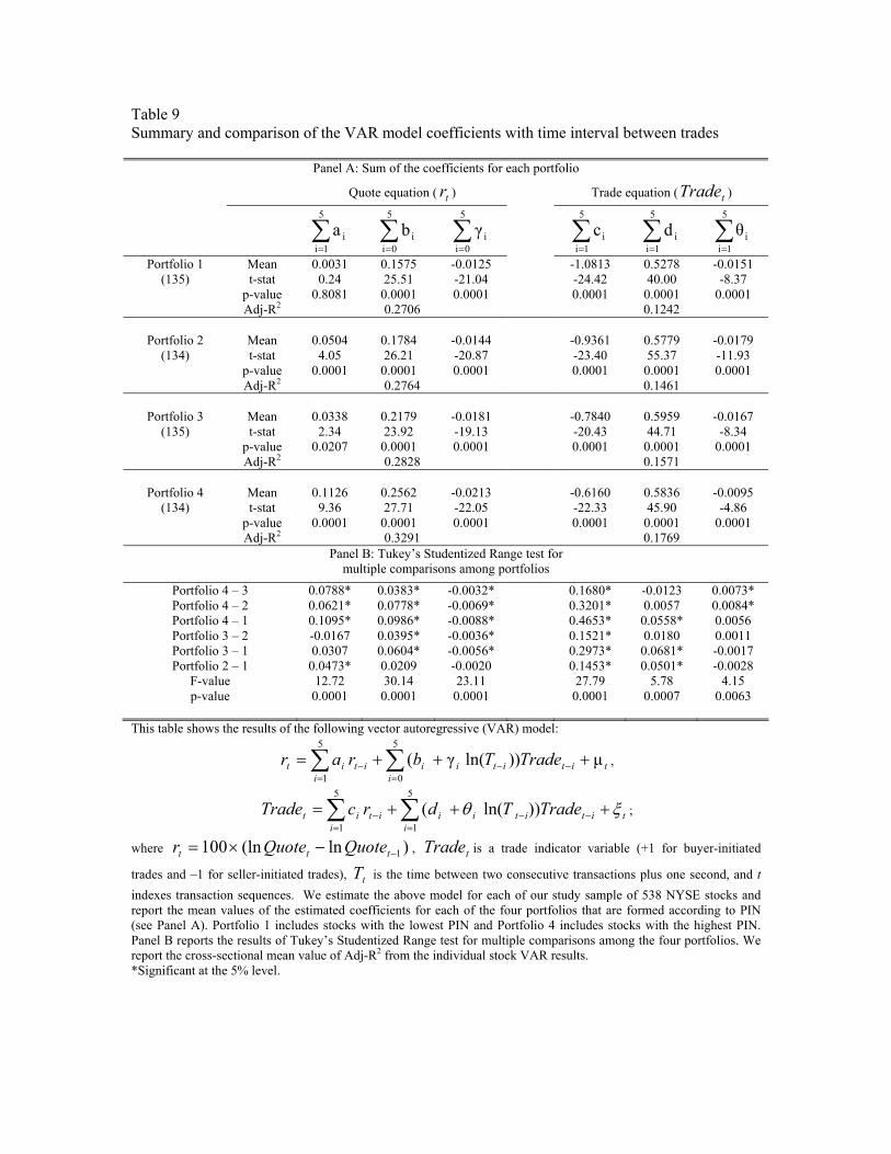
Table 9 Summary and comparison of the VAR model coefficients with time interval between trades

Panel A: Sum of the coefficients for each portfolio Quote equation ( tr ) Trade equation ( tTrade )

∑=

5

1iia ∑

=

5

0iib ∑

=

5

0iiγ

∑=

5

1iic ∑

=

5

1iid ∑

=

5

1iiθ

Portfolio 1 Mean 0.0031 0.1575 -0.0125 -1.0813 0.5278 -0.0151 (135) t-stat 0.24 25.51 -21.04 -24.42 40.00 -8.37

p-value 0.8081 0.0001 0.0001 0.0001 0.0001 0.0001 Adj-R2 0.2706 0.1242


p-value 0.0001 0.0001 0.0001 0.0001 0.0001 0.0001 Adj-R2 0.2764 0.1461

Portfolio 3 Mean 0.0338 0.2179 -0.0181 -0.7840 0.5959 -0.0167

(135) t-stat 2.34 23.92 -19.13 -20.43 44.71 -8.34 p-value 0.0207 0.0001 0.0001 0.0001 0.0001 0.0001 Adj-R2 0.2828 0.1571


p-value 0.0001 0.0001 0.0001 0.0001 0.0001 0.0001 Adj-R2 0.3291 0.1769


Portfolio 4 – 3 0.0788* 0.0383* -0.0032* 0.1680* -0.0123 0.0073* Portfolio 4 – 2 0.0621* 0.0778* -0.0069* 0.3201* 0.0057 0.0084* Portfolio 4 – 1 0.1095* 0.0986* -0.0088* 0.4653* 0.0558* 0.0056 Portfolio 3 – 2 -0.0167 0.0395* -0.0036* 0.1521* 0.0180 0.0011 Portfolio 3 – 1 0.0307 0.0604* -0.0056* 0.2973* 0.0681* -0.0017 Portfolio 2 – 1 0.0473* 0.0209 -0.0020 0.1453* 0.0501* -0.0028

F-value 12.72 30.14 23.11 27.79 5.78 4.15 p-value 0.0001 0.0001 0.0001 0.0001 0.0007 0.0063

This table shows the results of the following vector autoregressive (VAR) model:

tititii

iiti


0

5

1

+++= −−=

−=

∑∑ ,

titi

itiiiti


−−=

∑∑ ))ln((5

1

5

1;

where )ln(ln100 1−−×= ttt QuoteQuoter , tTrade is a trade indicator variable (+1 for buyer-initiated

trades and –1 for seller-initiated trades), tT is the time between two consecutive transactions plus one second, and t indexes transaction sequences. We estimate the above model for each of our study sample of 538 NYSE stocks and report the mean values of the estimated coefficients for each of the four portfolios that are formed according to PIN (see Panel A). Portfolio 1 includes stocks with the lowest PIN and Portfolio 4 includes stocks with the highest PIN. Panel B reports the results of Tukey’s Studentized Range test for multiple comparisons among the four portfolios. We report the cross-sectional mean value of Adj-R2 from the individual stock VAR results. *Significant at the 5% level.

information-based trading, price impact of trades,...

Documents