Information Asymmetry and the Timing of Capital Issuance: An International Examination

April M. Knill

and Bong Soo Lee

Abstract

Using issuance data across 50 countries from 1996 through 2009, we examine the role of information

asymmetry in market timing globally. We utilize a model that takes into account the possible feedback of

security issues to past market returns allowing us to ascertain whether timing of capital issuance around

the world is based on information asymmetry. We find evidence of both market timing and pseudo market

timing. The evidence for market timing is significantly stronger in international sub-samples with greater

levels of information asymmetry when capital issuance is measured by equity share. The evidence for

pseudo market timing is consistent across sub-samples when capital issuance is measured by changes in

equity issuance. These results suggest that information asymmetry in a market plays an important role in

the ability of managers to time capital issuance and that counter to the implications of extant literature,

market timing and pseudo market timing are not mutually exclusive, i.e., existence of one does not nullify

the other.

JEL classification: C53, G14, G15, G32,

Key words: equity issues, market timing, information asymmetry, international evidence

College of Business, The Florida State University, Rovetta Business Building, Tallahassee, FL 32306,

aknill@cob.fsu.edu, (tel) 850-644-2047, (fax) 850-644-4225

College of Business, The Florida State University, 251 Rovetta Business Building, Tallahassee, FL

32306, blee2@cob.fsu.edu, (tel) 850-644-4713, (fax) 850-644-4225

1

Information Asymmetry and the Timing of Capital Issuance:

An International Examination

Abstract

Using issuance data across 50 countries from 1996 through 2009, we examine the role of information

asymmetry in market timing globally. We utilize a model that takes into account the possible feedback of

security issues to past market returns allowing us to ascertain whether timing of capital issuance around

the world is based on information asymmetry. We find evidence of both market timing and pseudo market

timing. The evidence for market timing is significantly stronger in international sub-samples with greater

levels of information asymmetry when capital issuance is measured by equity share. The evidence for

pseudo market timing is consistent across sub-samples when capital issuance is measured by changes in

equity issuance. These results suggest that information asymmetry in a market plays an important role in

the ability of managers to time capital issuance and that counter to the implications of extant literature,

market timing and pseudo market timing are not mutually exclusive, i.e., existence of one does not nullify

the other.

JEL classification: C53, G14, G15, G32,

Key words: equity issues, market timing, information asymmetry, international evidence

2

Market timing and pseudo market timing theories differ fundamentally with respect to whether

market efficiency holds or not 1 and thus the literature implicitly assumes that market timing and pseudo

market timing are mutually exclusive ideas; proof of the existence of one nullifies the existence of the

other. Given the important role that information asymmetry plays in market timing, however, it makes

sense that the level of information asymmetry in a market would affect the likelihood that market timing

could occur. Depending on the relative information asymmetry in a given nation, managers may not be

able to exploit their superior knowledge. Conversely, in pseudo market timing, which uses a more

backward-looking approach, information asymmetry may not play an important role. Examining the U.S.

only, as many studies on market timing and pseudo market timing have done in the past, conceals the role

of information asymmetry in the timing of capital issuance. As such, the extant literature has heretofore

found evidence of one theory or the other, suggesting that they are mutually exclusive. We posit that

using a cross-section (i.e., international sample) is a more appropriate sample to examine the timing of

capital issuance in that it allows for diversity in information asymmetry, which in turn allows for evidence

of both market timing and pseudo market timing. We further posit that the patterns of this evidence may

be explained using information asymmetry.

Henderson et al. (2006) take a first step in examining the timing of capital-raising in an international

setting, finding evidence of both market timing and pseudo market timing in an international study. They

note that “estimates vary somewhat across regions” (p. 80). Indeed this is the case. Using equity share as

the determinant, only roughly half of the sub-samples analyzed show evidence of market timing and/or

pseudo market timing. As the intent of Henderson et al. (2006) is a preliminary examination of the world

1 Some studies find little evidence that IPOs and SEOs underperform the market on a risk-adjusted basis (e.g., Brav et al., 2000;

Eckbo et al., 2000; Mitchell and Stafford, 2000; Li and Zhao, 2003; and Butler et al., 2005). Gao et al. (2011) show that U.S.

IPOs from 1980-2009 underperform size- and book-to-market benchmarks when the pre-issue annual sales are less than $50M

($2009) by x%, but have insignificant positive abnormal performance when in the three years after issuing pre-issue sales are

above $50M. Chan et al. (2008) also report conditional underperformance. Butler et al. (2005) argue that the negative association

between equity issues and future aggregate stock returns is spurious. They show that the negative relation is primarily driven by

the strong positive correlation between market prices and the equity share surrounding the two structural breaks in U.S. economic

activities -- the Great Depression (1929-1931) and the oil crisis (1973-1974) periods -- and there is no out-of- sample predictive

power in the equity share variable.

3

market for raising capital, they do not attempt to examine why some evidence of both competing

hypotheses is found or why that evidence varies across nations. Our paper extends Henderson et al.

(2006) by exploring these issues. Combining the implications from the market timing, pseudo market

timing, and information asymmetry in capital issuance literatures, we explain the patterns in market

timing and pseudo market timing across 50 countries over the period 1996-2009. Specifically, we attempt

to explain patterns in the evidence of market timing and pseudo market timing as well as capital types

(i.e., the equity share, equity and debt).

Using an econometric model designed to carefully control for information asymmetry, we examine

the role of information asymmetry in the timing of capital issuance. We examine directly the role of

information asymmetry by ascertaining whether there is evidence of Granger causality in information-

based sub-samples. Based on such papers as Miller et al. (2008) and Anderson et al. (2009) who discuss

differences in information asymmetry in groups (country development and shareholder dispersion,

respectively), we create sub-samples based on information asymmetry: common law versus civil law

countries, strong versus weak investment profile, low versus high earnings management smoothing

countries, high versus low auditor presence countries, high versus low number of analysts countries, and

high versus low institutional investors countries. This allows us to better identify what environments

foster market timing (i.e., issuing equity before downturns in the market) and pseudo market timing (i.e.,

issuing after upturns in the market).2

The breadth and depth of our data arguably avoids the small sample bias discussed in prior literature.

Examining markets across 50 countries affords us sufficient heterogeneity to ascertain whether it is

possible that advocates of both market timing and pseudo market timing are correct. It also allows us to

examine what role, if any, information asymmetry (i.e., divergence from market efficiency) plays in

market timing around the globe.

2 Given that our international sample covers only fourteen years (1996 through 2009), we don’t pursue the issue of whether

market timing is real or a fiction being driven by structural breaks or other non-stationarities in the data.

4

In our analysis, we find greater evidence of market timing of the share of equity in sub-samples with

greater information asymmetry (i.e., civil law, weak investment profile, high earnings management

smoothing, low auditor and analyst presence as well as low institutional investor importance nations). In

support of Baker and Wurgler (2000; 2002), our findings suggest that the variation in the results found by

Henderson et al. (2006) are due to information asymmetry. We also find evidence of pseudo market

timing of equity issues. This evidence is found in all sub-samples, suggesting that information asymmetry

does not play a role in pseudo market timing of equity issues. This is quite intuitive since after return is

realized, information asymmetry is resolved. Interestingly, there is a role for information asymmetry in

pseudo market timing of debt issues. In particular, there exists evidence of pseudo market timing in sub-

samples with lower information asymmetry, suggesting that managers use backward-looking

consideration for this part of the capital structure.

Comprehensively, we find evidence of both market timing and pseudo market timing of equity issues

in sub-samples with greater levels of information asymmetry (i.e., equity share and changes in equity,

respectively), suggesting that both hypotheses have merit and that managers can use both forward- and

backward-looking strategies to optimize the timing of capital issuance.

The paper closest to ours in the literature is Henderson et al. (2006). Using extensive international

data, they find that firms all around the world are more likely to issue equity (debt) prior to periods of low

(high) stock (bond) market returns. However, the intent of Henderson et al. (2006) differs considerably

from ours. Henderson et al. provide an informative examination of capital issuance in an international

setting and find that issuers (pseudo) market time in an international setting. We extend Henderson et al.

(2006) by examining the role of information asymmetry in the patterns of both market and pseudo-market

timing.

The rest of the paper proceeds as follows. In Section I, we motivate the hypotheses, and in Section II,

we discuss the regression equations (i.e., Granger causality) we use in the test of market timing as well as

their relation to information asymmetry. In Section III, we describe our data with descriptive statistics and

various subsets of different countries. Section IV presents our main empirical results. Section V explores

5

the robustness of our results (e.g., excluding Australia, excluding simultaneous international offerings,

and looking at only IPOs and follow-on offerings), Section VI offers a final discussion, and finally

section VII concludes the paper.

I. Motivation

There are two explanations for underperformance by firms following equity offerings: market timing

and pseudo market timing. Market timing is a behavioral explanation pioneered by Baker and Wurgler

(2000) that suggests that stock prices periodically diverge from fundamental values, and that managers

take advantage of overpricing by selling stock or bonds to overly optimistic investors (e.g., Ritter, 1991;

Lerner, 1994; Loughran and Ritter, 1995, 2000; Hirshleifer, 2001).3 In their U.S.-based study, Flannery

and Rangan (2006) state that the market timing hypothesis asserts that managers routinely exploit

information asymmetries to benefit current shareholders.4,5

The notion that future returns can be predicted

from past prices flies in the face of market efficiency, and Schultz (2003) proposes a different explanation

for the same phenomenon. Schultz (2003) shows that underperformance by firms following equity

offerings is very likely to be observed ex-post in an efficient market and can be explained by a “pseudo”

market timing hypothesis (assuming that issuing volume follows a nonstationary process). The premise of

the hypothesis is that more firms issue equity at higher stock prices even though the market is efficient

and managers have no timing ability.

3 Early studies find that initial public offerings (IPOs) underperform relative to market indices and matching stocks after going

public (Ritter, 1991). Other studies find similar underperformance following seasoned equity offerings (SEOs) (e.g., Loughran

and Ritter, 1995; Spiess and Affleck-Graves, 1995; Lee, 1997; and Burch et al., 2004). See also Chen and Liang, 2006, who find

evidence of market timing ability in hedge funds, especially in bear and volatile markets. 4 See Sanders and Carpenter (2003) for a discussion of how stock repurchase programs, the opposite of equity issuance, is a

function of information asymmetry.

5 Consistent with this contention, a study by Chang et al. (2010) finds that the companies in a keiretsu (in Japan) cooperate with

each other to time equity issues (the specifics of which their investors are not aware) and that this market timing occurs more for

keiretsu firms than for standalone firms. Chemmanur and Simonyan (2010) find that firms issue putable convertibles when they

have valuable private information; firms without this information issue regular convertibles.

6

In a related literature, the role of information asymmetry in security issuance was first examined by

Myers and Majluf (1984). This seminal paper explained the importance of information in what type of

capital firms issue. Papers such as Dierkens (1991), Korajczyk et al. (1991, 1992), Bayless and

Chaplinsky (1996), Guo and Mech (2000) and Kennedy et al. (2006) extended this line of research by

asking the question whether information asymmetry affects more than just the type of capital. Given that

managers know more about the firm than investors, it is theoretically possible for managers to time the

issuance of capital to take advantage of stock prices that are overvalued. In this way, managers can

minimize their cost of capital, therefore maximizing the value of the firm.

While this research speaks to information asymmetry across time, it is theoretically possible that

differences in information asymmetry across markets can also affect a manager’s ability to time capital

issuance. Given insufficient levels of information asymmetry between managers and investors due to

characteristics of a nation (such as legal protection of investors, business stability, and accounting

standards such as earnings smoothing, the presence of Big 5 Accounting firms as well as analysts and the

importance of institutional investors), managers may not be able to exploit superior knowledge to reap the

financial reward of additional proceeds when their equity is over-valued. Market timing, therefore, may

only exist in nations where levels of information asymmetry are relatively high. Said formally:

H1: There is greater evidence of market timing (i.e., securities issuance’s predictive power of market

return) in international sub-samples with greater levels of information asymmetry.

Since ex post, investors have the same information as managers, information asymmetry should not

play a role when we test for evidence of pseudo market timing. Specifically, we should find similar

evidence of pseudo market timing across information asymmetry sub-samples around the world, at least

with regard to equity issues. Said formally, we hypothesize that:

7

H2: Evidence of pseudo market timing (i.e., market return’s predictive power of security issuance) is

similar across international sub-samples with different levels of information asymmetry.

Putting these two hypotheses together, we would expect to find evidence of both market timing and

pseudo market timing in sub-samples with greater information asymmetry and evidence only of pseudo

market timing in sub-samples with less information asymmetry.

II. Empirical Model

A. A test of asymmetric information based on causality tests (Sims test)

In this section, we provide a simple, parsimonious time-series model in which there is potential

information asymmetry between informed inside managers and outside investors so that we can

distinguish between market timing and pseudo market timing. In such a case, equity issue (or equity

share) decisions may contain (or convey) new information about future stock returns. 6 In fact, some

equity issue decisions may be information events (i.e., forward-looking), while others may be non-

information events (i.e., backward-looking) with respect to stock returns. The equity issue decision will

be related to future stock returns when it is an informative event under information asymmetry. The idea

is that, although informed inside managers and uninformed outside investors observe the same financial

variables such as current and past stock returns and fundamentals, uninformed outside investors may not

recover all the information which informed inside managers use in equity issue.7 Our model is very

useful because it provides a regression model that tests the predictive power of equity issue under

potential information asymmetry.

6 Here, we focus on the relation between equity issues (or equity share) and stock returns. However, the same logic

applies to the relation between debt issues and bond returns.

7 We can capture this intuition in a time-series concept of the non-invertibility of the moving average representation

[see Box and Jenkins (1976, p.69) and Granger and Newbold (1986, p.145)].

8

Here, we utilize a theorem in time-series econometrics, which states that any time-series process

has both invertible and non-invertible representations [see Fuller (1976, P. 64-66, Theorem 2.6.4)].

Although stock returns may follow a general ARMA (autoregressive moving average) process, for

expositional simplicity, we assume that uninformed outside investors, observing current and past stock

returns, infer a first-order moving average, MA(1), process of the returns: 8

Rt = (1 – L) ut, < 1.0 , (1)

where Rt is the stock return at time t, L is the lag (or backshift) operator (i.e., Ln Rt = Rt-n), and ut is white

noise with var(ut) = u2. The autocovariance functions (ACFs) for this return process are:

var(Rt) = (1 + 2) u

2,

cov(Rt, Rt-1) = - u2,

cov(Rt, Rt-k) = 0, for k 2. (2)

Conversely, suppose that informed inside managers, observing the same current and past stock

returns, infer the following MA(1) process of the returns:

Rt = (1 – -1

L) vt, < 1.0 , (3)

where vt is white noise with var(vt) = v2. The ACFs for this return process are:

var(Rt) = (1 + -2

) v2,

cov(Rt, Rt-1) = - -1

v2,

cov(Rt, Rt-k) = 0, for k 2. (4)

8 Any higher order representation of returns yields the same dynamic relations with more complicated computations.

9

Note that if we set v2 =

2 u

2, the ACFs in (2) and (4) are identical. Since the return process can be

identified in practice only by the observed ACFs, the identical ACFs imply that stock return processes in

(1) and (3) represent the same return process. That is, for a given return process, outside investors and

inside managers may infer different MA(1) processes.9 In addition, v

2 is smaller than u

2 because

v2 =

2 u

2, and < 1.0. (5)

This means that the variance of the one-step-ahead forecast error of the return process in (3) by

inside managers would be smaller than the corresponding variance of the return process in (1) by

uninformed outside investors. However, unlike the ut process, the vt process cannot be recovered by

uninformed investors from the information about current and past values of stock returns.10

In sum,

although both inside managers and outside investors observe the same (current and past) returns, under

information asymmetry informed inside managers with a larger information set t* = {Rt-j, vt-j, ut-j, for j

0} can forecast future returns better than uninformed investors with a smaller information set t = {Rt-j,

ut-j, for j 0}.

We can gain an important alternative insight by comparing the corresponding autoregressive

representations (ARR) of the moving average representations (MAR) of stock return processes {Rt} in (1)

and (3):

9 The return process in (1) with the innovation ut is an invertible MAR because the root of the determinant of the

MAR of Rt is greater than 1 (i.e., det [1- z] = 0, for z = -1). However, the return process with the innovations vt in

(3) is a non-invertible MAR because the root of the determinant is less than 1 (i.e., det [1- -1 z] = 0, for z = ).

10 This is because the process is not invertible.

10

Note that the innovations {ut} in the uninformed outside investors’ return process are backward-looking,

whereas the innovations {vt} in the informed inside managers’ return process are forward-looking.11

How is this information asymmetry between inside managers and outside investors related to the

dynamic relation between equity issue (or equity share) decisions and stock returns (i.e., the predictive

power of equity issues)? Suppose that inside managers have an informational advantage in that they can

forecast the firm’s future prospects better than uninformed investors by observing vt. If inside managers

use this information in their equity issue decisions, their equity issue (or equity share, St) decision will be

a function of the innovation vt that they observe but uninformed outside investors do not:

Then, by using vt in (6), the equity share variable, St, and stock return processes will be related as follows:

11

In practice, it would be more practical to posit the relation with an expectation operator that

j

t t j

j 1

v [ R ].tE

The innovations {ut} are represented by a square summable linear combination of current and past values of Rt’s

(i.e., ut lies in the space spanned by current and lagged Rt’s). However, the innovations {vt} are represented by a

square summable linear combination of future values of Rt’s (i.e., vt lies in the space spanned by future Rt’s). This is

because if we solve (3) backwards, the right-hand side is not square summable.

1 -1 -1 -1 1 j

t t t t j

j 1

v ( 1 L) R -( L )(1 L ) R R . (6)

0j

jt

j

t

1

t and,R RL) (1u

i 2

t t i t i t-i

i 0 i 0 i 0

f (v ) ( L ) v v , with . (7.1)iS

i i -1 1

t i t i t

i 0 i 0

i j

i t j j t j

i 0 j 1 j -

( L ) v ( L ) { (1 L) R }

( L )( R ) R , (7.2)

S

11

where j for j = -∞, …, -2, -1, 0, 1, 2, ….∞ is a function of i and j . That is, the equity share will be a

linear combination of future, current, and past returns; thus, it will be forward-looking. In practice, since

inside managers do not have perfect foresights, (7.2) will be

In contrast, suppose that inside managers do not have an informational advantage or they simply do

not make equity issue (or equity share) decisions based on their informational advantage. Then, the equity

share will be a function of ut , the innovation that uninformed outside investors observe,:

Then, by using ut in (6), equity share and stock return processes will be related as follows:

where k for k = 0, 1, 2, ….∞ is a function of i and j . That is, in this case, the equity share will only

reflect the past and current returns and will not be related to future returns; thus, it will be backward-

looking. To summarize, we have shown that under information asymmetry, informative equity issue (or

equity share) decision will be related to not only past and present returns but also future returns. In

contrast, in the absence of information asymmetry, non-informative equity issue (equity share) decision

will not be related to future returns.

A practical question is how we distinguish between the two -- informative and non-informative --

types of equity issue (or equity share) decisions. When an inside manager makes equity issue decision, if

it contains new information about future prospects of the firm (i.e., stock returns) that is not contained in

i i 1

t i t i t

i 0 i 0

i t-j k t-k

i 0 0 k 0

( L ) u ( L ) (1 L) R

( ) { R } R , (10) i j

j

S

L

i 2

t t i t i t-1

i 0 i 0 i 0

f ( u ) ( L ) u u , with . (9)iS

1

t j t j t j t j

j 0 j -

R + E [ R ]. (8) S

12

the current and past values of returns and equity issues, it is an informative (i.e., forward-looking) equity

issue and it is related to future returns. Otherwise, it is a non-informative (i.e., backward-looking) equity

issue. We can empirically test whether equity issue (or equity share) decisions are informative or not by

using the following proposition.

The equivalence of the two-sided regression in (7.2) with Granger-causality has been established

by Sims (1972, Theorem 2), which we restate in our context:

Proposition 1. Consider the following two-sided regression:

,m

t j t j t

j m

S R

(11)

where E(εt. Rt-j) = 0 for all j (= -m. …-1, 0, 1,… m). If the null hypothesis that all the coefficients of

future returns are zero (i.e., j = 0 for all j < 0 ) is rejected, then tS Granger-causes Rt.

That is, we can use the two-sided regression as a means of testing the predictability of equity issue (or

equity share) for market returns, and the finding of the predictive power of equity issue can be interpreted

based on information asymmetry. An intuition behind this test is that including lagged values of market

returns helps us to control for potential feedback in equity issue decisions.12

B. Empirical Model

In testing the predictive power of equity issues, existing studies use a regression of current market

return (Rt) on lagged equity share in new issues (St-1):

ttt SR 1 , (12)

12

It is interesting to note that, according to the pseudo-market timing story of Schulz (2003), both market timing and pseudo-

market timing hypotheses are consistent with past returns affecting issuance decisions, which is reflected in equation (11). On the

other hand, the market timing hypothesis suggests that we should observe post issuance returns, which is consistent with our

claim that issuance is related to future returns in equation (11).

13

where St = Et/(Et + Dt) is the equity share variable defined as the ratio of equity issue amount (Et) to the

sum of equity (Et) and debt issue amount (Dt).13

Baker et al. (2006) point out that this regression may not

be sufficient to differentiate the two hypotheses: market timing and pseudo-market timing hypotheses.

Instead, they characterize market timing as the tendency of firms to issue equity before low equity

market returns, and pseudo-market timing of Schultz (2003) as the tendency of firms to issue equity

following high returns.

Given the difference between the two competing views (i.e., whether managers are able to predict a

future stock price, or return, decline), one way to test the difference is to see whether equity issues help

better predict future decline in returns. Since both views agree that more equity issues tend to follow

higher stock prices, we also need to control for past stock price changes.

As discussed above, in our context, if equity issues (or equity shares) Granger-cause future stock

returns with a negative sign, then we can interpret this as evidence of equity issue containing additional

information that is not contained in past stock returns and as a result equity issues help better predict

future decline in returns. Then this can be used as evidence for the market timing view. If not, equity

issues do not contain additional information about future returns, and thus the pseudo market timing view

is supported.

Further, given potential information asymmetry between inside managers and outside investors, it is

more likely to be the case for samples and environments when and where the information asymmetry is

higher and more easily exploited by managers. The use of a Granger causality test across sub-samples of

disparate levels of information asymmetry can be a unique method of distinguishing between the two

views in an international setting.

Equivalently, the Granger causality in (11) can be tested by the null hypothesis that j = 0 for all j >

0 based on the following regression:

13 Domestic issues are used. In the robustness section, we will reexamine the base analysis excluding domestic issuances that

have simultaneous international issues to ensure that the timing of international issues does not bias results.

14

1 1

m m

t j t j j t j t

j j

R R S

. (13)

That is, we can use a one-sided Granger causality test in (13) as a means of testing the predictability of

the equity share for stock market returns (i.e., market timing), and the finding of the predictive power of

the equity share can be interpreted based on information asymmetry. The intuition behind this test is that

including lagged values of market returns helps us to control for potential feedback in equity issue

decisions. It is also interesting to note that Lucas and McDonald (1990) have developed an asymmetric

information model in an attempt to explain potential predictability of equity issues, although their

approach is very different from ours.

For thoroughness, we examine three measures for capital issuance previously examined in the

literature - the equity share in total new equity and debt issues, the change in equity issues, or change in

debt issues. 14

We use the following three regressions taking into account possible feedback of equity

(and/or debt) issues from past market returns:

1

1 1

m mE E

t i t i i t i t

i i

R R S

, (14)

2

1 1

,m m

E E

t i t i i t i t

i i

R R E

(15)

3

1 1

,m m

D D

t i t i i t i t

i i

R R D

(16)

14 Regarding the market timing of debt issues, Baker et al. (2003) find that managers have better foresight into debt market

innovations than other market participants so that managers successfully anticipate and time the market by their security issuance

choice. However, Butler et al. (2006) argue that the Baker et al. (2003) result is driven by a structural break in the data, and once

such non-stationarities are addressed, there is no in-sample predictive power of the long term share predictor variable.

In response to the claims of Butler et al. (2005) that the predictive power of the equity share is driven by small sample bias, Baker

et al. (2006) point out that aggregate pseudo-market timing is simply another name for the small-sample bias studied by

Stambaugh (1986, 1999) and others. Baker et al. (2006) demonstrate that small sample bias is in fact too small to explain the

predictive power. Therefore, the predictive power is indeed real.

15

where E

tR in (14) and (15) is the stock market return, D

tR in (16) is the bond market return (following

Henderson et al., 2006, we use 10-year interest rate swap rate),15

St is the equity share in total equity and

debt issues (= Et/(Et + Dt)), and itE ( itD )16

is the log difference in equity (debt) issues (i.e., growth in

equity/debt issues). Since this causality test can be interpreted as being based on information asymmetry

as discussed above, we interpret a finding of causal relation from equity issues to market return as

evidence of market timing of equity issues based on information asymmetry.

St, the equity share in total equity and debt issues, is said to Granger-cause the market return if we

reject:

H0: i = 0, for all i in (14).

In other words, the equity share Granger-causes the market returns if lagged equity shares can predict

current market returns, controlling for past returns. If the null H0: i = 0, for all i in (14) is rejected, we

find evidence of market timing using the equity share. This specification also allows us to test the net

(cumulative) effect of lagged equity shares on the market returns. Specifically, we test:

H0 :

1

m

i

i

= 0 in (14),

which allows us to test for the sign of the causal relation. If we find the net effect (sum of coefficients,

1

m

i

i

) is significantly negative, the sign of the causation is consistent with the expectation that managers

increase equity issues relative to debt in anticipation of a drop in market return (i.e., market timing).

15 Henderson et al. (2006) justify use of the swap rate of bond market interest rates since they are equivalent to the yield on a par

bond issued by the most-credit worthy buyer and are thus unaffected by default risk (Footnote #16; page 88).

16 The first difference in debt and equity issues is used to address the potential unit root in these issues (see Schultz, 2004,

Viswanathan and Wei, 2003 and Dahlquist and de Jong, 2008 for discussions on this).

16

Similarly, changes in equity (debt) issues Granger-cause stock (bond) market return if we reject H0:

i = 0, for all i in (15) ((16)), and the net effect of changes in equity (debt)17

issues on the market returns

can be examined by testing H0: 1

m

i

i

= 0 in (15) ((16)). If the null H0: i = 0, for all i in (15) ((16)), is

rejected, we find evidence for the market timing using equity (debt) issues. The market timing theory

anticipates the sign of the net effect 1

m

i

i

in (15) is negative, while the sign of the net effect 1

m

i

i

in

(16) is positive.

The premise of the pseudo-market timing is that more firms issue equity at higher stock prices even

though the market is efficient and managers have no timing ability. For the test of the pseudo-market

timing, the following regression equations are specified:

1

1 1

m mE

t i t i i t i t

i i

S R S

, (17)

2

1 1

m mE

t i t i i t i t

i i

E R E

, (18)

3

1 1

m mD

t i t i i t i t

i i

D R D

. (19)

Similarly, the equity shares (changes in equity issues or changes in debt issues) are Granger-caused by the

market returns if we reject H0: i = 0, for all i in (17) ((18) or (19)). The net effect of lagged market

returns on the equity shares (changes in equity issues or changes in debt issues) can be examined by

testing H0: 1

m

i

i

= 0 in (17) ((18) or (19)). If the null H0: i = 0, for all i in (17) ((18) or (19)) is rejected,

we find evidence for the pseudo-market timing using the equity shares (equity issues or debt issues). If we

17 Specifications using contemporaneous rates have also been examined with results qualitatively identical. They are available

upon request.

17

find the sign of the net effect (i.e., 1

m

i

i

) in (17) is positive, this implies that firms issue more equity

relative to debt following high returns on the market, which is consistent with the pseudo-market timing

theory. Similarly, the pseudo-market timing theory anticipates the sign of the net effect (i.e., 1

m

i

i

) in

(18) and (19) is positive and negative, respectively.

Under the pseudo market timing environment, more firms issue equity at higher stock prices even

though the market is efficient and managers have no market timing ability. As such, information

asymmetry is not a factor and we anticipate that the different level of the information asymmetry does not

make any difference between samples. However, under the market timing environment, information

asymmetry can be an important factor and we anticipate to see that samples with higher (or easier to

exploit) information asymmetry will show stronger evidence of the market timing.

To provide further evidence on the market timing by equity issues based on extensive international

data, we group countries as common law versus civil law countries, strong versus weak investment profile

countries, low versus high earnings management smoothing countries, high versus low auditor presence

countries, high versus low presence of analysts countries, and high versus low institutional investors

countries. Hence, if the market timing is primarily due to information asymmetry, we expect to find

greater evidence of market timing in civil law, weak investment profile, high earnings management

smoothing, low auditor and analyst presence as well as low institutional investor importance countries.

The use of these sub-samples is further substantiated in the next section.

III. Data and Descriptive Statistics

Issuance data are obtained from SDC Platinum Global New Issues from 01/01/1996 through

18

08/31/2009.18

Global new issues are not readily available prior to this era in SDC. We collect

observations for common stock, non-convertible debt, convertible debt, non-convertible preferred stock

and convertible preferred stock.19

Care is taken to note whether issuances are domestic or international.

International issuances are identified following the methodology of Gozzi, Levine, and Schmukler (2009)

and then dropped from the sample. Domestic issues are used in the analyses since it is these issuances that

would use local market returns for market timing (or pseudo market timing). Following Schultz (2003),

we exclude funds, investment companies and REITs (SIC codes 6722, 6726 and 6792) as well as

offerings by utilities (SIC codes 4911-4941) and banks (6000-6081). The total number of issuances

obtained through this dataset is 174,442, which includes 68,201 equity issuances and 106,241 debt

issuances. A detailed list of the issuances by country of origin (50 countries) and the average principal per

issue by country is given in Panel A of Table 1.

[Insert Table 1 here]

Stock return data is obtained from Thomson Financial’s Datastream. The most broadly defined

index in each country is obtained to represent the return of the market. The price indices are value-

weighted. Where available, the “all share” index is used. In lieu of the all share index, the next most

broadly defined index is obtained. This may be problematic where individual companies represented by

the issuance data are not included in the index. Using the most broadly defined index possible minimizes

this possibility and resulting biases would serve to work against the market timing hypothesis (versus

pseudo-market timing). Returns are collected in a monthly periodicity. A detailed list of these indexes is

provided in Panel B of Table 1.

18 As mentioned in the introduction, this fourteen-year term, although significant enough to perform empirical tests, is not long

enough to examine structural breaks in the data as in market timing examinations done in the United States. We assume that the

heterogeneity found in the cross-sectional data is significant enough that we do not pursue systematic structural breaks in the

data.

19 Mortgage and asset-backed securities as well as municipal bonds are not included to ensure consistency across countries where

information on these securities is not available.

19

Also collected from Datastream are the ten-year interest rate swap rates. Following Henderson et al.

(2006), we use these rates for our debt issuance analysis. This methodology limits the sample in that there

is limited or no data available for some of the 50 countries in our sample. Due to the number of lags in

our analysis and with the implementation of the Euro relative to our sample period, we use an eight-year

minimum length. Although admittedly somewhat arbitrary, the results are not sensitive to other cut-off

points. A list of sample averages for the countries included is provided in Panel B of Table 1.

Countries are dropped from the original SDC Platinum New Issues list only due to lack of

issuance observations in SDC Platinum or because return data is not available within Datastream.

Excluding these countries results in dropping approximately one percent of the overall dataset and is not

thought to bias the results in any significant way.

A. Issuance Information

Following the market timing literature, we use the “S ratio,” which is defined empirically as equity

principal (i.e., the amount issued) scaled by the sum of equity and debt principal (St = Et/(Et + Dt)), as one

of the predictors of market return. The data used to calculate this figure is obtained from the issuance

data. Other predictors include changes in equity and debt levels. We define this empirically as the log

difference in equity and debt issuance levels (separately) (∆Et and ∆Dt) and their lags.

B. Compilation of Data

Return data are carefully merged into the issuance data to ensure the maintenance of the relative time

period. To ascertain the impact of issuance on prior and subsequent returns, it is imperative that the time

period be matched carefully to ensure that the correct period is being measured. We follow Henderson et

al. (2006) by using monthly issuance data and calculate returns (in our case, quarterly) using a geometric

mean. With consideration of the Akaike Information criterion (1974) and the Schwarz Information

criterion (1978), we use four lags in the regressions.

20

C. Creation of Sub-samples

Sub-samples of nations in the analysis are determined through several means: legal origin,

investment profile, earnings management smoothing, Big 5 Auditor presence, number of analysts, and the

importance of institutional investors. Legal origin is used to examine the ultimate impact of the

importance of the development of a country’s legal system. This variable is chosen based on and derived

from the literature finding the importance of security law and investor protection such as La Porta et al.

(1997; 1998) and La Porta et al. (2006). Investment profile indices are derived from International Country

Risk Guide’s Investment Profile, which is a component that makes up their political risk index. The

investment profile indicates the level of general stability in business that is prevalent in a country; the

more (less) stability in a nation, the less (more) information asymmetry exists. 20

The index is derived

from data collected on nation’s contract viability, expropriation, profits repatriation, and payment

delays.21

The range of investment profiles is zero to twelve, with higher numbers reflecting less risk in

investment. The data is cross-sectional time-series.22

Following the accounting literature, several proxies for information asymmetry are used. As an

indicator of corporate transparency, we include an indicator of the level of earnings management (Leuz et

al., 2003), the presence of the Big 5 auditing firms (Bushman et al., 2004). As an indicator for how

information is gathered, we include both the average number of analysts (Chang et al., 2000; Bushman et

al., 2004) and the importance of institutional investors (Beck et al., 1999). Data for these variables are at a

country level.

In unreported results, we also performed analysis in country development (G10 versus nonG10) and

opacity.23

Results are qualitatively identical to those in this paper and are left out for brevity but are

20

See Chen et al. (2010) for a discussion on how political-connectedness affects information asymmetry.

21 http://www.prsgroup.com/ICRG_Methodology.aspx

22 This implies that countries are not restricted from moving from one category to another throughout its time series.

23 The basis for empirical opacity is a risk premium created by Pricewaterhouse Coopers reflecting the level of information

transference possible in a market. Opacity is relevant based on its effect on information asymmetry in the market (Bhattacharya et

al., 2003). Data for these variables are at a country level.

21

available upon request.

In constructing our data set, each country data are stacked very much like panel data analysis. A

similar stacking scheme is used in Vuolteenaho (2002), who examines the driver of stock return volatility

for U.S. firms.24

Definitions of all variables and sub-samples are found in the Appendix. Values for the

bases of these sub-samples may be found in Table 2.

[Insert Table 2 here]

Bifurcation of the data is substantiated using proxies of information asymmetry from Leuz (2003).

The two values used are market capitalization and total value traded. These values come from World

Bank’s World Development Indicators. Leuz uses these proxies to establish the level of information

asymmetry in a nation. Specifically, higher values of these two proxies indicate a lower level of

information asymmetry. The data is cross-sectional time-series. To substantiate the sub-samples as being

different with regard to information asymmetry, we provide a difference in means test of the proposed

sub-samples. Table 3 shows the results of these tests. The results clearly indicate that civil law, weak

investment profile, high earnings management smoothing, low auditor/analyst presence, and low

institutional investor importance nations have a statistically significant higher level of information

asymmetry. Regardless of the proxy used for information asymmetry or the sub-sample examined (one

exception is earnings management smoothing in the difference in means for total value traded/GDP),

24 When we use cross sectional data together with time series data, potential heterogeneous characteristics in cross section data

can be an important issue. Once we fail to consider potential heterogeneity in the cross sectional data, we may treat all data

containing either a causal relation as a group or no causal relation as a group. However, in our case, we are mainly interested in

whether different groups (e.g., common law vs. civil law group, etc.) have different causal relations as a group rather than

knowing which countries have a causal relation among the group. Therefore, for our purpose, a panel causality test can be

implemented assuming homogenous causal relation in each group and we naturally focus on the difference between each group

as a whole, rather than some part of each group. In sum, while we are using a panel data, given our main focus, it is sufficient to

pool the data for each group and implement a causal relation test assuming a homogeneous relation for each group (see, for

example, Kónya, 2006; Granger, 1969; Hsiao, 1982; Holtz-Eakin, Newey, and Rosen, 1988; Judson and Owen, 1999; Hartwig,

2009a, b).

22

there is a statistically significant difference in the means of these sub-samples, which substantiates their

use in our analysis.

[Insert Table 3 here]

IV. Empirical Results

A. Market Timing

Results for market timing show a distinction between the sub-samples. Using equity shares, Panel A

of Table 4 shows greater evidence of Granger causality for all of the sub-samples with greater information

asymmetry (i.e., civil law, weak investment profile, high earnings smoothing, lower auditor and analyst

presence and low institutional investor importance nations) than for the sub-samples with less information

asymmetry (i.e., common law, strong investment profile, low earnings smoothing, high auditor and

analyst presence, and high institutional investor importance). Specifically, in specifications (2), (4), (6),

(8), (10), and (12), we find that the null hypothesis that lagged equity shares, S (St = Et/(Et + Dt)), as a

group is insignificant (i.e., γi = 0 for all i) is rejected. Though statistical significance varies across sub-

samples, all are significant. In the one lower information asymmetry sub-sample where we find evidence

of Granger causality (i.e., low earnings management smoothing), this evidence is weaker than that of its

counterpart. As suggested in the motivation section, greater evidence of Granger causality in greater

information asymmetry sub-samples is interpreted to mean that in these subsamples, it is easier for

insiders to exploit the information that they have relative to outsiders.25

Collectively, this evidence suggests that the equity share Granger-causes returns in the sub-samples

with more information asymmetry. Their net effect (sum of coefficients,

4

1

i

i

) is significantly negative in

all of the aforementioned sub-samples. The sign of the causation is consistent with the expectation that

the share of equity capital would increase before a drop in market return (i.e., market timing). These

25Chow tests, though statistically significant for the paired sub-samples in Table 4, are not included because they do not affect

Granger causality test results and their interpretation.

23

results are consistent with those in Henderson et al. (2006). However, the results offer further insight into

why evidence of market timing is found in some countries but not in others – information asymmetry.

[Insert Table 4 here]

The results of Panel B are not as impressive as those in Panel A. In looking at the evidence as to

whether the change in equity issues (ΔE) has some predictive power for market returns, we find that there

is only conclusive evidence of Granger causality in one sub-sample: low auditor presence. There is

statistical significance for only the χ2(1) test results for seven sub-samples but these are not very

meaningful since the χ2(4) results, which tell us if there is evidence of Granger causality, are not

statistically significant, except for the low auditor presence sub sample. Though the comprehensive

evidence here is considerably weak, one of the six proxies for information asymmetry shows evidence

consistent with the equity share results in Panel A.

In Panel C, we find less than consistent predictive power in the change in debt issues (ΔD) as well.

There are no sub-samples that show evidence of Granger Causality. Three sub-samples, however, show

evidence of a statistically significant positive net effect (sum of coefficients,

4

1

i

i

): high auditor

presence, high analyst presence, and high institutional importance nations. It is interesting to note that all

three of these sub-samples have less information asymmetry, suggesting perhaps that managers in nations

where a less significant information advantage is possible try to market time using debt instruments. That

said, the lack of statistical significant evidence of Granger causality weakens the impact of this evidence.

The lack of evidence is not surprising once we consider the fact that the literature on the market timing of

debt issuances (e.g., Barclay and Smith, 1995; Guedes and Opler, 1996; Baker, Greenwood, and Wurgler,

2003) suggests that it is the maturity of existing debt or the issuances that is of importance, not the

amount. Since we do not document the maturity of the debt issued and look at rates on only ten-year

interest rate swaps, this characteristics of debt is completely ignored, suggesting that the literature in this

area is less comparable to the results found herein. The results on market timing of debt issues in

24

Henderson et al. (2006) are likewise weak.26

Since we use the same proxy for debt market interest rates, it

is comforting to find similar results.

Collectively, the evidence is not as strong for ΔE and ΔD as for S. These findings support the

contentions of Baker and Wurgler (2000), who suggest that equity share is a strong predictor of (U.S.)

stock market returns. The evidence of a vital role of information asymmetry in environments with greater

information asymmetry for equity share suggests that managers in these environments use market timing

to achieve capital structure goals. This, along with the less consistent results for changes in equity and

debt issues, suggests that the role of information asymmetry in changes in equity and debt individually is

unclear.

B. Pseudo-market Timing

As expected, the results found in Panel A of Table 5 show no pattern of evidence of pseudo market

timing in equity share St regardless of the level of information asymmetry. This is intuitive in the sense

that outsiders are privy to the same information as insiders (where returns are concerned) ex post. The

sub-sample with low number of analysts shows a significant pseudo market timing in equity share, but its

cumulative net effect on the market return is insignificant.

Panel B of Table 5 demonstrates strong evidence of market return Granger-causing the change in

equity. Importantly, all of the sub-samples show evidence of Granger causality, suggesting that

information asymmetry does not play a distinctive role. Once again, we expect that this should be the case

ex post. The significant positive cumulative impact suggests that firms issue equity following high returns

on the market, which is consistent with the pseudo-market timing theory. As discussed above, according

to the pseudo market timing hypothesis, more firms issue equity at higher stock prices even though the

market is efficient and managers have no market timing ability. As such, information asymmetry is not a

factor and we anticipate that the different level of the information asymmetry does not make any

difference between sub-samples.

26 Our specification is most comparable to equation (12) of Henderson et al. (2006; p. 91).

25

Evidence of debt market return Granger-causing change in debt issuances in our sub-samples is

provided in Panel C of Table 5. Interestingly, the results show evidence of pseudo market timing of debt

issuances primarily in sub-samples with lower levels of information asymmetry. The sign of the causality,

as established by the cumulative significance, is negative, suggesting that debt issuances follow

downturns in the market. This evidence is consistent with the work of Erel et al. (2010) and Gomes and

Phillips (2010), both of which suggest that debt securities, which are less informationally sensitive, are

used in times when there are greater levels of information asymmetry.

[Insert Table 5 here]

V. Robustness

A. Excluding Australia and the United States

Table 6 presents the results of robustness tests. Cross-country studies that examine equity issues

often exclude Australia due to its unique form of equity rights issues. This form of offering allows the

existing shareholders to decide whether they would like to accept a certain amount of shares based on a

pre-determined ratio at a price lower than market value. These equity offerings are typically excluded (or

the entire country in the cross-country sample) as rights issues affect firm fundamentals such as share

capital, book value per share, earnings per share, and the liquidity of the stock. Since the inclusion of

these observations could potentially bias the results, we provide the results after excluding Australia. In

looking at the table, darker shading or unshaded boxes indicate changes from the base results. Darker

shading indicates that statistical significance in the table is increased from the base results. An unshaded

box represents lost statistical significance from the base results. Panel A shows that excluding Australia

only changes the results slightly in the pseudo-market timing tests. Results overall substantiate those in

the base analysis and do not suggest that our base results are spurious based on the inclusion of Australia.

Critics of international empirical studies often cite the influence of the United States on results since

it is a powerful outlier in most studies. As such, we exclude the United States from our analysis in Panel

26

B. The vast majority of results remain, though it is clear that the United States is influential. For example,

we find evidence of Granger causality in strong investment profile nations as well as nations with a high

analyst presence using equity share in the market timing analysis (these regions are shaded in a darker

grey to represent increased significance from the base results). That said, in every information asymmetry

bifurcation, sub-samples with higher information asymmetry still see stronger results, both in terms of

statistical and economic significance. The qualitative results regarding market timing are unchanged when

we exclude the United States. Results for pseudo market timing are also different from those in the base

analysis, suggesting that the United States is relevant to the sample. The vast majority of the differences

are found in the changes in debt issuances. Instead of finding evidence of Granger Causality in sub-

samples with lower information asymmetry, we actually find evidence of Granger Causality in three sub-

samples with greater information asymmetry. The results suggest that the United States is responsible for

the information asymmetry pattern in the pseudo market timing analysis. The weak results for pseudo

market timing of debt issues suggest that information asymmetry once again does not play a major role.

[Insert Table 6 here]

B. Excluding Simultaneous International Offerings

Since it is conceivable that market considerations across country border might contribute to any

timing decisions, we exclude all issuances that involve simultaneous international offerings to ensure that

these considerations are not biasing our base results. Doing so yields largely consistent results, which are

seen in Panel C of Table 6. Though there are some differences in the market timing results using equity

share, the stronger results in the sub-samples with more information asymmetry are sufficient to maintain

the conclusions of the analysis in this paper.

C. IPOs and Follow-on Offerings

Since several studies distinguish among initial public offerings (IPOs) and follow-on offerings (e.g.,

SEOs), we re-examine the base analysis on these sub-samples. This comparison is particularly relevant

27

since as Alti (2006, p. 1682) states, “The IPO market constitutes a natural laboratory to analyze market

timing [since] investors face more uncertainty and a higher degree of asymmetric information when

valuing IPO firms than they face in the case of mature public companies. Hence, IPOs offer more room

for misvaluation, which is at the root of timing considerations”.

The results for these analyses are found in Panels D and E of Table 6. The results of this bifurcation

support the findings of Frank and Goyal (2003; 2009), in particular, the preference of small firms (most

likely those in the IPO sub-sample seen in Panel D) for equity. This isn’t surprising given that IPOs

involve equity issuance. This manifests in more statistical significance across sub-samples in the change

in equity issuance specifications versus those with equity share. In contrast, the results for changes in

equity issuances in the market timing panel of Panel E (SEO’s) are less consistent with those of equity

share above it in the panel. This divergence suggests that preference for equity type plays a role in the

changes of specific security types. Interestingly, Panel D shows some evidence of a role for information

asymmetry in pseudo market timing of equity share and changes in equity issuances for IPOs. Though

these results are seemingly inconsistent with those prior, we recall that insiders definitely have an

informational advantage in these cases, even ex post. The amount of underpricing and the resulting true

value of the firm is still an uncertainty in the months subsequent to the IPO.27

Revelation of this

information by insiders is constrained by the lock-up period for insiders.28

This is also consistent with the

results of Dahlquist and de Jong (2008), who find diminished evidence of pseudo market timing in a

sample of IPOs.

VI. Future Research

The data used in the analysis are as exhaustive as possible given availability. That said, worldwide

27 The amount of underpricing can vary from country to country. See, for example, Boulton et al. (2010), who find that the level

of corporate governance in a nation influences the level of IPO underpricing.

28 See Arthurs et al. (2009) for a discussion of how the agreed upon length of the lock-up period is important with regard to

signaling quality to investors.

28

data on securities issuance and debt market interest rates are sure to improve going forward. Though the

results of equity share and changes in equity issuances are not likely to change, results of changes in debt

issuances may change based on the availability of swap rates. That said, results using market rates for

changes in debt issuances (i.e., how changes in debt issuances are affected through capital structure

concerns) largely validate those using swap rates suggesting that these also will not likely change based

on availability of data going forward. These results are available upon request.

This research begs further analysis of the timing of international issues. In this study, we explicitly

limit the sample to examine domestic issuances with domestic market index returns. Given the increase in

international listings, it would be interesting, however, to examine timing of international issues. Though

econometrically challenging, burgeoning globalization and the mobility of capital suggest that this is an

important topic for study. The inferior information of foreign investors could offer additional

opportunities for managers to time capital issuance so as to minimize their cost of capital.

VII. Concluding Remarks

The role of information asymmetry in managerial choice of securities (i.e., pecking order) and market

timing (i.e., on a time dimension) have been explored in the literature. We extend the literature to

consider the role of information asymmetry in market timing cross-sectionally. Specifically, we examine

whether market timing (and pseudo market timing) is more prevalent in international sub-samples with

greater levels of information asymmetry.

Existing studies use a regression of market returns on a lagged equity share variable to find evidence

of the market timing of equity issues. We argue, as in Baker et al. (2006), that this simple regression is

not effective in distinguishing between the market timing and pseudo-market timing hypotheses. We

provide and implement an alternative regression model based on Granger causality test idea, which helps

us distinguish between the two hypotheses. The model not only takes into account equity issues’ possible

feedback to past market returns but also is based on information asymmetry between inside managers and

29

outside investors. Empirically, we extend the existing literature by examining an extensive dataset of

international data.

Using a Granger causality framework, we find extensive evidence of both market timing and pseudo-

market timing in a sample which spans 50 countries over the period 1996 through 2009. The direction of

these causalities is in line with the respective theories. Analysis done on international sub-samples of the

data based on the level of information asymmetry reveals that information asymmetry is a key component

of a firm’s ability to market time issues with equity share being the best predictor. Among different

market types, we find substantial evidence of market timing of equity share in civil law, weak investment

profile, high earnings management smoothing, low auditor and analyst presence, as well as low

institutional investor importance markets, and evidence of pseudo-market timing of changes in equity in

all sub-samples. Results also reveal that information asymmetry does not play a role in a firm’s ability to

pseudo market time issues.

Collectively, the results of this paper help to explain the divergence in market timing and pseudo

market timing in extant literature. Specifically, the results confirm that market timing and pseudo market

timing are not mutually exclusive and that information asymmetry helps to explain the patterns in

evidence found in prior studies.

30

References

Akaike, H., 1974, “A New Look at the Statistical Identification Model,” IEEE Transactions on

Automated Control, 19, 716–723.

Alti, A., 2006, “How Persistent is the Impact of Market Timing on Capital Structure?” The Journal of

Finance 61, 1681–1710.

Anderson, R., A. Duru, and D. Reeb, 2009, “Founders, Heirs, and Corporate Opacity in the United States,”

Journal of Financial Economics 92, 205-222.

Arthurs, J., L. Busenitz, Hoskisson, R., and R. Johnson, 2009, “Signaling and Initial Public Offerings:

The Use and Impact of the Lockup Period,” Journal of Business Venturing 24, 360-372.

Baker M., R. Greenwood, and J. Wurgler, 2003, “The Maturity of Debt Issues and Predictable Variation

in Bond Returns,” Journal of Financial Economics 70, 261-291.

Baker M., R. Taliaferro, and J. Wurgler, 2006, “Predicting Returns with Managerial Decision Variables:

Is There a Small Sample Bias?” Journal of Finance 61, 1711-1730.

Baker M. and J. Wurgler, 2000, “The Equity Share in New Issues and Aggregate Stock Returns,” Journal

of Finance 55, 2219–2257.

Baker M. and J. Wurgler, 2002, “Market Timing and Capital Structure,” Journal of Finance 57, 1-32.

Barclay, M. and C. Smith, 1995, “The Maturity Structure of Corporate Debt,” Journal of Finance 50,

609–631.

Bayless, M. and S. Chaplinsky, 1996, “Is There a Window of Opportunity for Seasoned Equity

Issuance?” The Journal of Finance 51, 253-278.

Beck, T., A. Demirguc-Kunt, and R. Levine, 1999, “A new Database on Financial Development and

Structure,” World Bank Economic Review 14, 597-605.

Bhattacharya U., H. Daouk, and M. Welker, 2003, “The World Price of Earnings Opacity,” The

Accounting Review 78, 641-678.

Boulton, T., S. Smart, and C. Zutter, 2010, “IPO Underpricing and International Corporate Governance,”

Journal of International Business Studies 41, 206–222.

Box, G. E. P. and G. M. Jenkins, 1976. Time Series Analysis: Forecasting and Control, Holden-Day.

Brav A., C. Geczy, and P. Gompers, 2000, “Is the Abnormal Return following Equity Issuances

Anomalous?” Journal of Financial Economics 56, 209–249.

Burch T., W. Christie, and V. Nanda, 2004, “Do Firms Time Equity Offerings? Evidence from the 1930s

and 1940s,” Financial Management 33, 5-23.

Bushman, R., J. Piotroski, and A. Smith, 2004, “What Determines Corporate Transparency?” Journal of

Accounting Research 42, 207-252.

31

Butler A., G. Grullon, and J. Weston, 2005, “Can Managers Forecast Aggregate Market Returns?”

Journal of Finance 60, 963-986.

Butler A., G. Grullon, and J. Weston, 2006, “Can Managers Successfully Time the Maturity Structure of

Their Debt Issues?” Journal of Finance 61, 1731-1758.

Chan, Cooney, Kim Singh, 2008, “The IPO Derby: Are there Consistent Losers and Winners on this

Track?” Financial Management 37, 45-79.

Chang, J., T. Khann, and K. Palepu, 2000, “Analyst Activity around the World.” HBS Strategy Unit

Working Paper No. 01-061.

Chang, X., H. Gilles, M-S. Chia, and L. Tam, 2010, “Conglomerate Structure and Capital Market

Timing,” Financial Management 39, 1307-1338.

Chemmanur, T. and K. Simonyan, 2010, “What Drives the Issuance of Putable Convertibles: Risk-

Shifting, Asymmetric Information, or Taxes? Financial Management 39, 1027-1067.

Chen B. and Y. Liang, 2006, “Do Market Timing Hedge Funds Time the Market?” Journal of Financial

and Quantitative Analysis forthcoming.

Chen, C., Y. Ding, and C. Kim, 2010, “High-level Politically Connected Firms, Corruption, and Analyst

Forecast Accuracy around the World,” Journal of International Business Studies 41, 1505–1524.

Dahlquist, M. and F. deJong, 2008, “Pseudo Market Timing: A Reappraisal” Journal of Financial and

Quantitative Analysis 43, 547-579.

Dierkens, N., 1991, “Information Asymmetry and Equity Issues,” Journal of Financial and Quantitative

Analysis 26, 181-199.

Durnev, A., V. Errunza, and A. Molchanov, 2009, “Property Rights Protection, Corporate Transparency,

and Growth,” Journal of International Business Studies 40, 1533–1562.

Eckbo E., R. Masulis, and O. Norli, 2000, “Seasoned Public Offerings: Resolution of the ‘New Issues

Puzzle’,” Journal of Financial Economics 56, 251–291.

Erel, I., B. Julio, W. Kim, and M. Weisbach, 2010, “Macroeconomic Conditions and the Structure of

Securities,” The Ohio State Univ. and NBER, Dice Center WP 2009-6 (Fisher College of Business)

Flannery, M. and K. Rangan, 2006, “Partial Adjustment toward Target Capital Structures,” Journal of

Financial Economics 79, 469–506.

Frank, M. and V. Goyal, 2003, “Testing the Pecking Order Theory of Capital Structure,” Journal of

Financial Economics 67, 217-248.

Frank, M. and V. Goyal, 2009, “Capital Structure Decisions: Which Factors are Reliably Important?,”

Financial Management 38, 1-37.

Fuller W., Introduction to Statistical Time Series, New York: John Wiley, 1976.

32

Gao, X., J. Ritter and Z. Zhu, 2011, “Where Have All of the IPOs Gone?” Working Paper, University of

Florida.

Gomes, A. and G. Phillips, 2010, “Why do Public Firms Issue Public and Private Equity, Debt and

Convertibles?” Working Paper, Washington University.

Gozzi, J., R. Levine, and S. Schmukler, 2009, “Patterns of International Capital Raisings,” Journal of

International Economics 80, 45-57.

Granger, C., 1969, “Investigating Causal Relations by Econometric Models and Cross-Spectral

Methods,” Econometrica 37, 424-438.

Granger, C. W. J. and P. Newbold, 1986. Forecasting Economic Time Series, 2nd

edition, Academic Press

Guedes, J. and T. Opler, 1996, “The Determinants of The Maturity of Corporate Debt Issues,” Journal of

Finance 51, 1809–1833.

Guo, L. and T. Mech, 2000, “Conditional Event Studies, Anticipation, and Asymmetric Information: The

Case of Seasoned Equity Issues and Pre-issue Information Releases,” Journal of Empirical Finance

7, 113-141.

Hartwig, J., 2009a, “Is Health Capital Formation Good for Long-Term Economic Growth? – Panel

Granger-Causality Evidence for OECD Countries,” Journal of Macroeconomics (forthcoming).

Hartwig, J., 2009b, “A Panel Granger-Causality Test of Endogenous Vs. Exogenous Growth,” ETH

Zurich KOF Swiss Economic Institute, KOF Working Papers No. 231, July 2009.

Henderson B., N. Jegadeesh, and M. Weisbach, 2006, “World Markets for Raising New Capital,” Journal

of Financial Economics 82, 63-101.

Hirshleifer, D., 2001, “Investor Psychology and Asset Pricing,” Journal of Finance 56, 1533-1597.

Holtz-Eakin, D., W. Newey, and H. Rosen, 1988, “Estimating Vector Autoregressions with

Panel Data,” Econometrica 56, 1371–1395.

Hsiao, C., 1982, “Autoregressive Modeling and Causal Ordering of Economic Variables,” Journal of

Economic Dynamics and Control 4, 243-259.

Huang, R. and J. Ritter, 2009, “Testing Theories of Capital Structure and Estimating the Speed of

Adjustment,” Journal of Financial and Quantitative Analysis 44, 237-271.

Judson, R. and Owen, A., 1999, “Estimating Dynamic Panel Data Models: A Guide for

Macroeconomists,” Economic Letters 65, 9-15.

Kennedy, D., R. Sivakumar and K. Vetzal, 2006, “The Implications of IPO Underpricing for the Firm and

Insiders: Tests of Asymmetric Information Theories,” Journal of Empirical Finance 13, 49-78.

Kónya, L., 2006, “Exports and Growth: Granger Causality Analysis on OECD Countries with a Panel

Approach,” Economic Modelling 23, 978-992.

33

Korajczyk, R., D. Lucas, and R. McDonald, 1991, “The Effect of Information Releases on the Pricing

And Timing of Equity Issues,” The Review of Financial Studies 4, 685-708.

Korajczyk, R., D. Lucas, and R. McDonald, 1992, “Equity Issues with Time-varying Asymmetric

Information,” Journal of Financial and Quantitative Analysis 27, 397-417.

La Porta R., F. Lopez-de-Silanes, and A. Shleifer, 2006, “What Works in Securities Laws?” Journal of

Finance 61(1), 1-32.

La Porta R., F. Lopez-de-Silanes, A. Shleifer, and R. Vishny, 1997, “Legal Determinants of External

Finance,” Journal of Finance 52, 1131-1150.

La Porta R., F. Lopez-de-Silanes, A. Shleifer, and R. Vishny, 1998, “Law and Finance,” Journal of

Political Economy 106, 1113-1155.

Lee I., 1997, “Do Firms Knowingly Sell Overvalued Equity?” Journal of Finance 52, 1439-1466.

Lerner, J., 1994, “Venture Capitalists and the Decision to Go Public,” Journal of Financial Economics

35, 293-316.

Leuz, C., 2003, “IAS versus U.S. GAAP: Information Asymmetry-based Evidence from Germany's New

Market,” Journal of Accounting Research 41, 445-472

Leuz, C., D. Nanda, and P. Wysocki, 2003, “Investor Protection and Earnings Management: An

International Comparison,” Journal of Financial Economics 69, 505-527.8

Li X. and X. Zhao, 2003, “Is There Abnormal Return after Seasoned Equity Offerings?” Working paper,

Ohio State University.

Loughran T. and J. Ritter, 1995, “The New Issues Puzzle,” Journal of Finance 50, 23–51.

Loughran, T. and J. Ritter, 2000, “Uniformly Least Powerful Tests of Market Efficiency,” Journal of

Financial Economics 55, 361-390.

Lucas D. and R. McDonald, 1990, “Equity Issues and Stock Dynamics,” Journal of Finance 45, 1019-

1043.

Miller, S., D. Li, L. Eden, and M. Hitt, 2008, “Insider Trading and the Valuation of International Strategic

Alliances in Emerging Stock Markets,” Journal of International Business Studies 39, 102-117.

Mitchell M. and E. Stafford, 2000, “Managerial Decisions and Long-Term Stock Price Performance,”

Journal of Business 73, 287-320.

Myers, S. and N. Majluf, 1984, “Corporate Financing and Investment Decisions When Firms Have

Information that Investors Do Not Have,” Journal of Financial Economics 13,187-221.

Ritter J., 1991, “The Long-run Performance of Initial Public Offerings,” Journal of Finance 46, 3-27.

Sanders, G. and M. Carpenter, 2003, “Strategic Satisficing? A Behavioral-Agency Theory Perspective on

Stock Repurchase Program Announcements,” Academy of Management Journal 46, 160-178.

34

Schultz P., 2003, “Pseudo-market Timing and the Long-run Underperformance of IPOs,” Journal of

Finance 58, 483–517.

Schultz P., 2004, “Pseudo Market Timing and the Stationarity of the Event-Generating Process,” Working

Paper, University of Notre Dame.

Schwarz G., 1978, “Estimating the Dimension of a Model,” Annals of Statistics 6, 461-464.

Sims C., 1972, “Money, Income, and Causality,” American Economic Review 62, 540-552.

Spiess K. and J. Affleck-Graves, 1995, “Underperformance in Long-run Stock Returns Following

Seasoned Equity Offerings,” Journal of Financial Economics 38, 243-267.

Stambaugh R., 1986, “Bias in Regression with Lagged Stochastic Regression,” Working Paper.

University of Chicago.

Stambaugh R., 1999, “Predictive Regressions,” Journal of Financial Economics 54, 375-421.

Viswanathan, S. and B. Wei, 2003, “Endogenous Events and Long Run Returns,” Working paper, Duke

University.

Vuolteenaho, T., 2002, “What Drives Firm-level Stock Returns?” Journal of Finance 57, 233–264.

35

Appendix A. Variable Definitions

Variable Definitions

Common legal origin An indicator variable that equals one if a nation is of British legal origin and zero otherwise. Source:

La Porta et al. (1997;1998)

Civil legal origin An indicator variable that equals one if a nation is of German or French legal origin and zero

otherwise. Source: La Porta et al. (1997;1998)

Investment Profile

An index that measures the general level of business stability in a nation and is derived from data on contract viability, expropriation, profits repatriation, and payment delays in a nation. The range of

investment profiles is zero to twelve, with higher numbers reflecting less risk in investment. Source:

International Country Risk Guide (PRS Group)

Earnings management

smoothing

An index from 2 (low smoothing) to 28.3 (high smoothing) of the level of earnings management

occurs in a nation. Source: Leuz et al., 2003

Auditor presence An index from 1 (low) to 4 (high) indicating the percent of a nation’s firms audited by the Big 5

accounting firms (i.e., quartiles). Source: Bushman et al., 2004

Analyst presence Number of analysts following a nation’s largest 30 firms. Source: Bushman et al., 2004; Chang et

al., 2000

Institutional investors Indicates the importance of institutional investors in a nation – proxied by the average of total assets

in pooled investment, scaled by that nation’s GDP. Source: Beck et al., 1999

Market return The log difference of the price index from time t+1 to time t. Source: DataStream

Equity share (S) The natural log of the equity principal scaled by the sum of equity and debt principal. Source: SDC

Platinum

Change in equity (∆E) The log difference in the equity principal issues from time t to t-1. Source: SDC Platinum

Change in debt (∆D) The log difference in the debt principal issues from time t to t-1. Source: SDC Platinum

36

Table 1. Data characteristics

This table provides information on both the number/amount of issuances (Panel A) and the indices (Panel B) used in the analysis. Issuance data

are obtained from SDC Platinum from 1996-2009. Equity issuance includes IPOs, SEOs, SPACs, REITs and closed-end funds. Index returns and

interest rate swap rates are obtained from DataStream. A “.” indicates no available data for a given country.

Panel A. Issuances by country

Number of

equity issuances

Number of

debt issuances

Total number of

issuances

Avg principal/yr

($ mil)

Argentina 88 210 298 161.82

Australia 13,812 593 14,405 28.34

Austria 102 68 170 460.90

Belgium 174 38 212 450.42

Brazil 242 757 999 211.86

Canada 8,902 1987 10,889 85.02

Chile 232 489 721 57.07

China 1,377 355 1,732 151.20

Colombia 52 565 617 52.10

Czech Republic 9 3 12 286.29

Denmark 234 30 264 198.77

Ecuador 4 79 83 19.17

Egypt 96 4 100 129.37

Finland 216 60 276 231.68

France 1,236 596 1,832 371.36

Germany 1,067 561 1,628 431.19

Greece 231 56 287 537.00

Hong Kong 2,966 425 3,391 55.12

Hungary 20 31 51 242.69

India 1,973 2,305 4,278 31.56

Indonesia 265 366 631 83.03

Ireland 82 15 97 232.57

Israel 44 7 51 122.39

Italy 415 250 665 990.60

Japan 5,651 6,008 11,659 125.19

Luxembourg 16 3 19 291.67

Malaysia 1,525 1,352 2,877 40.05

Mexico 136 794 930 181.95

Netherlands 276 77 353 294.05

New Zealand 204 57 261 59.59

Norway 373 41 414 130.43

Pakistan 34 19 53 82.37

Peru 8 547 555 26.94

Philippines 177 118 295 147.49

Poland 221 45 266 168.95

Portugal 94 71 165 482.53

Russian Fed 37 5 42 387.87

Singapore 1,109 889 1,998 49.41

South Africa 78 24 102 182.99

South Korea 3,770 10,355 14,125 36.92

Spain 212 176 388 625.69

Sri Lanka 19 0 19 65.30

Sweden 500 203 703 142.12

Switzerland 242 501 743 205.07

Taiwan 1,150 1,983 3,133 42.22

Thailand 564 565 1,129 64.08

Turkey 61 0 61 328.27

United Kingdom 7,219 3,127 10,346 153.45

United States 10,581 69,346 79,927 156.86

Venezuela 78 83 161 160.88

Total 68,201 106,241 174,442 150.60

*Average

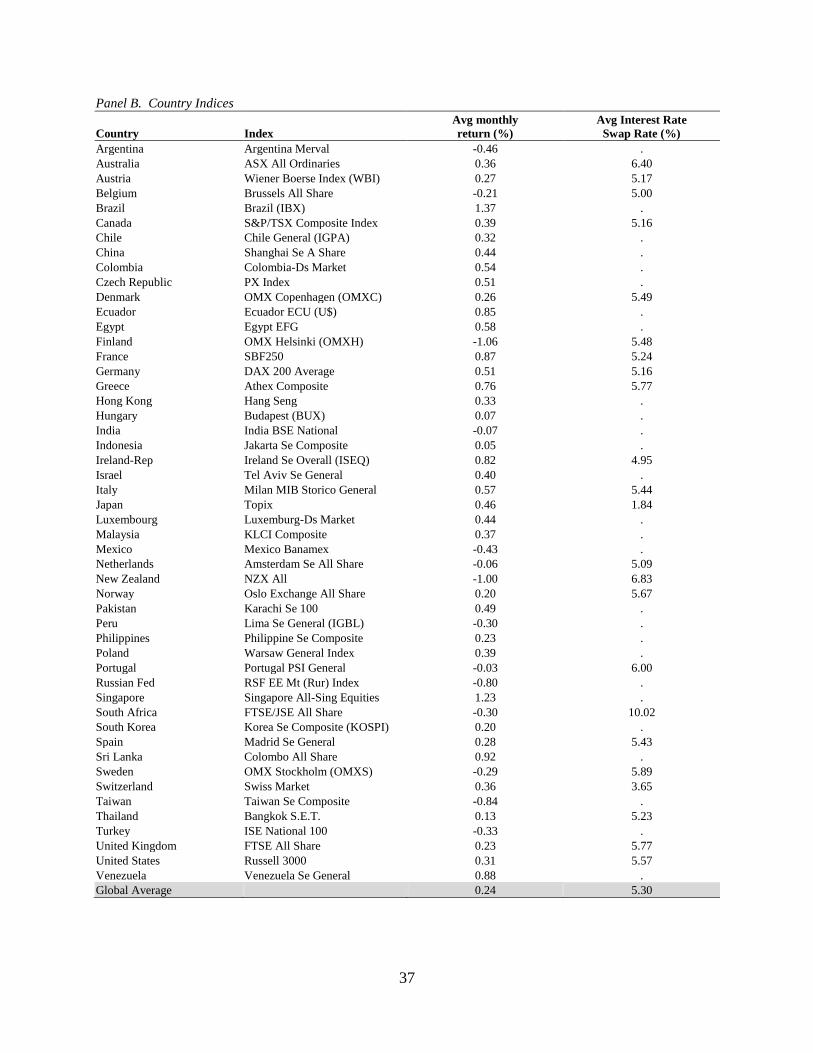
37

Panel B. Country Indices

Country Index

Avg monthly

return (%)

Avg Interest Rate

Swap Rate (%)

Argentina Argentina Merval -0.46 .

Australia ASX All Ordinaries 0.36 6.40

Austria Wiener Boerse Index (WBI) 0.27 5.17

Belgium Brussels All Share -0.21 5.00

Brazil Brazil (IBX) 1.37 .

Canada S&P/TSX Composite Index 0.39 5.16

Chile Chile General (IGPA) 0.32 .

China Shanghai Se A Share 0.44 .

Colombia Colombia-Ds Market 0.54 .

Czech Republic PX Index 0.51 .

Denmark OMX Copenhagen (OMXC) 0.26 5.49

Ecuador Ecuador ECU (U$) 0.85 .

Egypt Egypt EFG 0.58 .

Finland OMX Helsinki (OMXH) -1.06 5.48

France SBF250 0.87 5.24

Germany DAX 200 Average 0.51 5.16

Greece Athex Composite 0.76 5.77

Hong Kong Hang Seng 0.33 .

Hungary Budapest (BUX) 0.07 .

India India BSE National -0.07 .

Indonesia Jakarta Se Composite 0.05 .

Ireland-Rep Ireland Se Overall (ISEQ) 0.82 4.95

Israel Tel Aviv Se General 0.40 .

Italy Milan MIB Storico General 0.57 5.44

Japan Topix 0.46 1.84

Luxembourg Luxemburg-Ds Market 0.44 .

Malaysia KLCI Composite 0.37 .

Mexico Mexico Banamex -0.43 .

Netherlands Amsterdam Se All Share -0.06 5.09

New Zealand NZX All -1.00 6.83

Norway Oslo Exchange All Share 0.20 5.67

Pakistan Karachi Se 100 0.49 .

Peru Lima Se General (IGBL) -0.30 .

Philippines Philippine Se Composite 0.23 .

Poland Warsaw General Index 0.39 .

Portugal Portugal PSI General -0.03 6.00

Russian Fed RSF EE Mt (Rur) Index -0.80 .

Singapore Singapore All-Sing Equities 1.23 .

South Africa FTSE/JSE All Share -0.30 10.02

South Korea Korea Se Composite (KOSPI) 0.20 .

Spain Madrid Se General 0.28 5.43

Sri Lanka Colombo All Share 0.92 .

Sweden OMX Stockholm (OMXS) -0.29 5.89

Switzerland Swiss Market 0.36 3.65

Taiwan Taiwan Se Composite -0.84 .

Thailand Bangkok S.E.T. 0.13 5.23

Turkey ISE National 100 -0.33 .

United Kingdom FTSE All Share 0.23 5.77

United States Russell 3000 0.31 5.57

Venezuela Venezuela Se General 0.88 .

Global Average 0.24 5.30

38

Table 2. Sub-sample Characteristics

Common/Civil Law countries refer to those countries with the respective legal origins. The investment profile indicates the level of general

stability in business that is prevalent in a country. Earnings management smoothing (EMS) is an index from 2 (low smoothing) to 28.3 (high smoothing) of the level of earnings management occurs in a nation. Auditor Presence is an index from 1 (low) to 4 (high) indicating the percent

of a nation’s firms audited by the Big 5 accounting firms (i.e., quartiles). Analyst Presence is the average number of analysts following a nation’s

largest 30 firms. Institutional Investor indicates the importance of institutional investors in a nation – proxied by the average of total assets in pooled investment, scaled by that nation’s GDP. Figures are averaged over the term 1996-2009. A “.” indicates no available data for a given

country.

Country

Common

Law

Investment

Profile EMS

Auditor

Presence

Analyst

Presence

Institutional

Investor

Argentina 0 6.85 . . 12.73 .

Australia 1 10.23 4.8 4 12.3 0.103

Austria 0 10.11 28.3 3 8.63 0.109

Belgium 0 10.14 19.5 3 15.33 0.059

Brazil 0 6.99 . 3 16.1 0.184

Canada 1 8.95 5.3 4 16.9 .

Chile 0 10.32 . 4 5.53 0.069

China 0 7.31 . . . .

Colombia 0 8.93 . 3 3.31 .

Czech Republic 0 10.04 . . . .

Denmark 0 9.84 16 4 12.87 0.033

Ecuador 0 6.12 . . . .

Egypt 0 6.50 . . . .

Finland 0 10.46 12 4 14.9 0.013

France 0 10.50 13.5 3 23.2 0.371

Germany 0 10.52 21.5 4 32.4 0.135

Greece 0 9.87 28.3 1 6.1 0.047

Hong Kong 1 10.12 19.5 4 25 .

Hungary 0 9.50 . . . .

India 1 7.79 19.1 1 11.9 0.072

Indonesia 0 6.63 18.3 . . .

Ireland-Rep 1 10.77 . 4 5.43 0.262

Israel 1 9.45 . 0 3.19 0.123

Italy 0 10.22 24.8 4 21.57 0.072

Japan 0 9.71 20.5 4 14.87 .

Luxembourg 0 11.96 . 4 0 .

Malaysia 1 8.21 14.8 3 19.9 .

Mexico 0 9.86 . 3 18.53 .

Netherlands 0 10.83 16.5 4 29.53 0.156

New Zealand 1 11.53 . 4 8.87 .

Norway 0 11.50 5.8 4 12.83 0.038

Pakistan 1 7.63 17.8 2 3.4 .

Peru 0 8.15 . . 8.1 .

Philippines 0 8.88 8.8 1 10.87 .

Poland 0 10.64 . . . .

Portugal 0 10.54 25.1 3 5.33 0.101

Russian Fed . 8.84 . . . .

Singapore 1 11.02 21.6 4 20.9 .

South Africa 1 10.38 5.6 4 7.4 0.035

South Korea 0 8.62 26.8 . . .

Spain 0 11.14 18.6 4 22.73 0.163

Sri Lanka 1 . . . 2.4 .

Sweden 0 7.83 6.8 4 20.6 0.097

Switzerland 0 9.65 22 3 19.97 0.155

Taiwan 0 10.57 22.5 2 6.8 .

Thailand 1 8.50 18.3 3 9.77 .

Turkey 0 8.13 . 1 7.97 .

United Kingdom 1 11.90 7 4 20.1 0.126

United States 1 10.89 2 4 30.23 0.225

Venezuela 0 4.56 . 3 1.67 0.067

Table 3. Difference in Means

Common/Civil Law countries refer to those countries with the respective legal origins. The investment profile indicates the level of general stability in business that is prevalent in a country. Earnings management smoothing (EMS) is an indication of the level of earnings management occurs in a nation. Auditor Presence is an index from 1 (low) to 4 (high) indicating the percent of a nation’s firms

audited by the Big 5 accounting firms (i.e., quartiles). Analyst Presence is the number of analysts following a nation’s largest 30 firms. Institutional Investor indicates the importance of institutional

investors in a nation – proxied by the average of total assets in pooled investment, scaled by that nation’s GDP. Market capitalization is the aggregate value of a nation’s stock market. Total value traded is the aggregate value of the stocks traded in a nation. Observations are country-month and are based on the maximum number of observations included in the base analysis in Table 4 (N=4,818). Full

sample (4,045) does not equal 4,818 due to missing observations of market capitalization and total value traded.

Characteristic tested N

Market

capitalization

(% of GDP)

Difference test

statistic

Market

capitalization

(current $’s)

Difference

test statistic

Total value

traded (% of

GDP)

Difference test

statistic

Total value

traded

(current $’s)

Difference test

statistic

Full sample 4,045 94.00 1.12e+12 74.60 1.58e+12

Common legal origin 1,160 146.19 79.55***

2.29e+12 1.71e+12***

107.85 50.67***

3.44e+12 2.84e+12***

Civil legal origin 2,212 66.64 5.72e+11 57.17 5.98e+11

Strong Investment Profile 2,873 101.18 28.75***

1.36e+12 8.53e+11***

92.78 43.34***

1.80e+12 1.25e+11***

Weak investment Profile 1,790 72.43 5.08e+11 49.45 5.49e+11

Low earnings smoothing 1,537 108.14 5.32*

2.08e+12 1.41e+12***

96.62 2.39

2.92e+12 2.21e+12***

High earnings smoothing 1,967 102.79 6.63e+11 94.23 7.05e+11

High auditor presence 2,298 116.90 40.64***

1.73e+12 1.37e+12***

98.62 44.01***

2.32e+12 2.02e+12***

Low auditor presence 1,568 76.26 3.55e+11 54.61 2.93e+11

High number of analysts 2,963 111.44 52.11***

1.50e+12 1.41e+12***

96.57 72.80***

1.93e+12 1.89e+12***

Low number of analysts 1,082 59.33 8.95e+10 23.77 4.64e+10

High institutional investor 2,864 105.32 26.77***

1.48e+12 1.21e+12***

86.50 34.84***

1.92e+12 1.67e+12***

Low institutional investor 1,181 78.55 2.62e+11 51.66 2.19e+11

Table 4. Market Timing The following regression equation is specified:

4 4

1

1 1

,E E

t i t i i t i t

i i

R R S

in Panel A,

where E

tR is the stock return for month t, St is the ratio of the (equity principal/(equity principal + debt principal)) in month t. Common/Civil Law countries refer to those countries with the respective

legal origins. The investment profile indicates the level of general stability in business that is prevalent in a country. Earnings management smoothing (EMS) is an index from 2 (low smoothing) to 28.3

(high smoothing) of the level of earnings management occurs in a nation. Auditor Presence is an index from 1 (low) to 4 (high) indicating the percent of a nation’s firms audited by the Big 5 accounting

firms (i.e., quartiles). Analyst Presence is the number of analysts following a nation’s largest 30 firms. Institutional Investor indicates the importance of institutional investors in a nation – proxied by

the average of total assets in pooled investment, scaled by that nation’s GDP. The 2 (4) tests the null hypothesis that each lagged coefficient of St is zero. The 2 (1) tests the null hypothesis that the sum

of lagged coefficients of St is zero. Standard errors are given in brackets. *, **, *** indicate significance levels of 10, 5, and 1 percent, respectively. Shaded cells indicate evidence of significant test

results.

Panel A. Equity Share Dependent Variable = Rt

Legal

Origin Investment Profile

Earnings Management

Smoothing

Big 5

Auditors Presence

Number of

Analysts

Institutional

Investors

Common Civil Strong Weak Low High High Low High Low High Low

1 2 3 4 5 6 7 8 9 10 11 12

REt-1 0.410*** 0.212*** 0.244*** 0.248*** 0.375*** 0.273*** 0.302*** 0.205*** 0.335*** 0.174*** 0.286*** 0.166***

[0.029] [0.018] [0.018] [0.023] [0.026] [0.021] [0.020] [0.023] [0.019] [0.025] [0.018] [0.028]

REt-2 0.126*** 0.02 0.048*** 0.043* -0.003 0.123*** 0.029 0.048** 0.051*** 0.02 0.053*** -0.004

[0.029] [0.018] [0.017] [0.023] [0.025] [0.021] [0.020] [0.022] [0.019] [0.024] [0.017] [0.027] RE

t-3 -0.432*** -0.244*** -0.262*** -0.306*** -0.334*** -0.317*** -0.316*** -0.278*** -0.321*** -0.249*** -0.293*** -0.272***

[0.029] [0.018] [0.017] [0.023] [0.025] [0.022] [0.021] [0.023] [0.019] [0.024] [0.017] [0.028]

REt-4 0.108*** 0.028 0.032* 0.046* 0.131*** 0.019 0.130*** -0.021 0.100*** -0.016 0.021 0.082***

[0.030] [0.018] [0.018] [0.024] [0.026] [0.022] [0.021] [0.023] [0.020] [0.024] [0.018] [0.029]

St-1 -0.228 -0.411** -0.390** -0.433* -0.474** -0.448** -0.227 -0.641*** -0.353** -0.705*** -0.335** -0.855***

[0.269] [0.169] [0.156] [0.239] [0.238] [0.178] [0.171] [0.216] [0.167] [0.232] [0.154] [0.278] St-2 -0.26 -0.518*** -0.238 -0.734*** -0.661*** -0.516*** -0.063 -0.697*** -0.306* -0.537** -0.304** -0.705**

[0.256] [0.172] [0.154] [0.240] [0.236] [0.177] [0.167] [0.221] [0.163] [0.238] [0.155] [0.274] St-3 -0.007 -0.144 -0.03 -0.077 0.17 0.021 -0.173 -0.111 -0.117 -0.105 -0.016 -0.463*

[0.254] [0.171] [0.155] [0.238] [0.235] [0.177] [0.166] [0.223] [0.164] [0.233] [0.154] [0.280]

St-4 0.273 -0.152 -0.039 0.179 0.3 0.097 -0.085 0.188 0.036 0.077 0.033 -0.014 [0.260] [0.166] [0.150] [0.237] [0.239] [0.172] [0.165] [0.213] [0.164] [0.224] [0.152] [0.269]

Constant 0.289 1.079*** 0.780*** 1.034*** 0.802** 0.781** 0.714** 1.117*** 0.781*** 1.219*** 0.664*** 1.988***

[0.343] [0.292] [0.282] [0.360] [0.397] [0.307] [0.299] [0.386] [0.261] [0.424] [0.253] [0.537] Observations 1,160 2,868 3,022 1,796 1,537 2,116 2,298 1,723 2,691 1,509 3,013 1,187

# Countries 14 35 44 38 13 18 20 18 21 20 29 12

Model χ2 435.38 346.01 429.16 305.6 406.82 434.98 439.18 264.37 580.24 186.87 576.18 150.64

χ2 (4): S 2.19 13.61*** 7.80 10.86** 11.20** 12.63** 3.51 15.76*** 7.78 11.51** 7.33 14.59***

(p-value) 0.70 0.00 0.10 0.03 0.02 0.01 0.48 0.00 0.10 0.02 0.12 0.00

χ2 (1): S 0.27 10.17*** 4.30** 4.35** 2.13 4.46** 2.52 5.89** 5.12** 5.60** 3.63* 10.32***

(p-value) 0.60 0.00 0.04 0.04 0.14 0.03 0.11 0.02 0.02 0.02 0.06 0.00 Sum of Coef. -0.22 -1.22*** -0.70** -1.06** -0.67 -0.85** -0.55 -1.26** -.74** -1.27** -0.62* -2.04***

41

Table 4. Market Timing (cont.)

Panel B. Changes in Equity

Dependent Variable = Rt

Legal

Origin Investment Profile

Earnings Management

Smoothing

Big 5

Auditors Presence

Number of

Analysts

Institutional

Investors

Common Civil Strong Weak Low High High Low High Low High Low

1 2 3 4 5 6 7 8 9 10 11 12

REt-1 0.411*** 0.214*** 0.244*** 0.250*** 0.368*** 0.276*** 0.303*** 0.209*** 0.337*** 0.178*** 0.287*** 0.177***

[0.029] [0.018] [0.018] [0.023] [0.025] [0.021] [0.020] [0.023] [0.019] [0.025] [0.018] [0.028]

REt-2 0.128*** 0.021 0.050*** 0.044* -0.002 0.120*** 0.033 0.049** 0.054*** 0.018 0.055*** -0.003

[0.029] [0.018] [0.017] [0.023] [0.025] [0.021] [0.020] [0.022] [0.019] [0.024] [0.017] [0.027]

REt-3 -0.425*** -0.243*** -0.258*** -0.301*** -0.331*** -0.315*** -0.310*** -0.273*** -0.316*** -0.250*** -0.289*** -0.271***

[0.029] [0.018] [0.017] [0.024] [0.025] [0.022] [0.021] [0.023] [0.019] [0.024] [0.017] [0.028]

REt-4 0.108*** 0.028 0.032* 0.049** 0.131*** 0.024 0.132*** -0.015 0.102*** -0.013 0.023 0.087***

[0.030] [0.019] [0.018] [0.024] [0.026] [0.022] [0.021] [0.023] [0.020] [0.024] [0.018] [0.029]

∆Et-1 -0.001 0.000 -0.003** 0.000 -0.002 -0.002 -0.003** -0.015* -0.003* -0.008 -0.003* -0.011

[0.002] [0.004] [0.002] [0.005] [0.002] [0.004] [0.001] [0.009] [0.002] [0.007] [0.002] [0.010]

∆Et-2 -0.003 -0.001 -0.004** -0.005 -0.003 -0.009* -0.003** -0.028** -0.004** -0.011 -0.004* -0.024*

[0.002] [0.005] [0.002] [0.006] [0.002] [0.005] [0.002] [0.012] [0.002] [0.008] [0.002] [0.014]

∆Et-3 -0.002 -0.004 -0.005** -0.006 -0.003** -0.007 -0.004** -0.020* -0.004** -0.004 -0.004** -0.014

[0.002] [0.005] [0.002] [0.006] [0.002] [0.005] [0.002] [0.012] [0.002] [0.008] [0.002] [0.014]

∆Et-4 -0.001 -0.003 -0.002 -0.005 -0.001 -0.008** -0.002 -0.020** -0.002 -0.009 -0.002 -0.013

[0.002] [0.004] [0.001] [0.004] [0.001] [0.004] [0.001] [0.009] [0.001] [0.006] [0.001] [0.010]

Constant 0.136 0.379* 0.276* 0.486* 0.287 0.249 0.292** 0.440* 0.284* 0.463* 0.282* 0.537*

[0.183] [0.194] [0.149] [0.248] [0.180] [0.183] [0.144] [0.263] [0.148] [0.272] [0.157] [0.292]

Observations 1,160 2,868 3,022 1,796 1,537 2,116 2,298 1,723 2,691 1,509 3,013 1,187

# Countries 14 35 44 38 13 18 20 18 21 20 29 12

Model χ2 436.09 332.26 428.58 295.39 397.03 429.32 442.99 256.35 579.06 179.66 574.04 139.48

χ2 (4): ∆E 2.14 0.96 6.90 1.86 4.79 7.34 7.02 8.66* 6.06 5.03 5.35 4.51

(p-value) 0.71 0.92 0.14 0.76 0.31 0.12 0.14 0.07 0.20 0.28 0.25 0.34

χ2 (1): ∆E 1.56 0.31 5.63** 0.92 2.84* 3.56* 6.00** 5.74** 4.95** 1.89 4.80** 2.42

(p-value) 0.21 0.58 0.02 0.34 0.09 0.06 0.01 0.02 0.03 0.17 0.03 0.12

Sum of Coef. -0.01 -0.01 -0.01** -0.02 -0.01* -0.03* -0.01** -0.08** -0.01** -0.03 -0.012** -0.06

42

Table 4. Market Timing (cont.)

Panel C. Changes in Debt

Dependent Variable = Rt

Legal

Origin Investment Profile

Earnings Management

Smoothing

Big 5

Auditors Presence

Number of

Analysts

Institutional

Investors

Common Civil Strong Weak Low High High Low High Low High Low

1 2 3 4 5 6 7 8 9 10 11 12

RDt-1 0.256*** 0.165*** 0.244*** 0.211*** 0.233*** 0.219*** 0.224*** 0.221*** 0.233*** 0.217*** 0.316*** 0.147***

[0.041] [0.026] [0.021] [0.047] [0.027] [0.028] [0.022] [0.037] [0.023] [0.037] [0.024] [0.032]

RDt-2 -0.044 0.054** 0.115*** -0.073 0.039 0.105*** 0.043* 0.114*** 0.103*** 0.017 0.139*** -0.058*

[0.041] [0.026] [0.021] [0.047] [0.027] [0.028] [0.022] [0.038] [0.022] [0.037] [0.024] [0.032]

RDt-3 -0.110*** -0.137*** -0.205*** -0.115** -0.188*** -0.203*** -0.189*** -0.180*** -0.230*** -0.135*** -0.301*** -0.110***

[0.042] [0.025] [0.021] [0.047] [0.027] [0.028] [0.023] [0.037] [0.023] [0.037] [0.025] [0.030]

RDt-4 -0.058 -0.102*** -0.001 -0.125*** -0.056** -0.019 -0.053** -0.019 -0.006 -0.077** 0.081*** -0.175***

[0.042] [0.025] [0.021] [0.048] [0.027] [0.028] [0.022] [0.037] [0.022] [0.037] [0.025] [0.031]

∆Dt-1 0.000 0.000 0.000* 0.00 0.000 0.000 0.000 0.000 0.000* 0.001 0.000 0.000

[0.000] [0.000] [0.000] [0.000] [0.000] [0.000] [0.000] [0.001] [0.000] [0.001] [0.000] [0.002]

∆Dt-2 0.000 0.000 0.00 0.001** 0.000 0.000 0.000 0.003 0.000* 0.003 0.000* 0.001

[0.000] [0.000] [0.000] [0.000] [0.000] [0.000] [0.000] [0.002] [0.000] [0.002] [0.000] [0.002]

∆Dt-3 0.000 0.000 0.000* 0.00 0.000 0.000 0.000 0.002 0.000* 0.003 0.000* 0.002

[0.000] [0.000] [0.000] [0.000] [0.000] [0.000] [0.000] [0.002] [0.000] [0.002] [0.000] [0.002]

∆Dt-4 0.000 0.000 0.00 0.00 0.000 0.000 0.000 0.001 0.000 0.001 0.000 0.001

[0.000] [0.000] [0.000] [0.000] [0.000] [0.000] [0.000] [0.001] [0.000] [0.001] [0.000] [0.002]

Constant -0.073* -0.065*** -0.062*** -0.115** -0.070*** -0.070*** -0.069*** -0.072*** -0.064*** -0.080** -0.053*** -0.106***

[0.043] [0.021] [0.014] [0.056] [0.024] [0.021] [0.019] [0.028] [0.016] [0.038] [0.015] [0.035]

Observations 551 1,310 2,175 382 1,283 1,194 1,848 709 1,884 673 1,706 851

# Countries 8 15 23 16 11 11 16 7 15 8 14 9

Model χ2 69.54 114.49 302.62 57.58 178.14 142.56 239.31 86.42 276.85 72.32 372.76 91.92

χ2 (4): ∆D 3.72 0.62 5.87 6.61 3.49 0.58 4.03 4.45 4.78 2.43 4.17 1.10

(p-value) 0.44 0.96 0.21 0.16 0.48 0.97 0.40 0.35 0.31 0.66 0.38 0.89

χ2 (1): ∆D 2.60 0.00 2.48 1.62 2.58 0.12 2.85* 1.64 3.78* 1.68 3.57* 0.34

(p-value) 0.11 0.95 0.12 0.20 0.11 0.72 0.09 0.20 0.05 0.19 0.06 0.56

Sum of Coef. 0.00 0.00 0.00 0.00 0.00 0.00 0.00* 0.01 0.00* 0.01 0.00* 0.00

43

Table 5. Pseudo-market Timing The following regression equation is specified:

4 4

1

1 1

,E

t i t i i t i t

i i

S R S

in Panel A,

where E

tR is the stock return for month t, St is the ratio of the (equity principal/(equity principal + debt principal)) in month t. Common/Civil Law countries refer to those countries with the respective

legal origins. The investment profile indicates the level of general stability in business that is prevalent in a country. Earnings management smoothing (EMS) is an index from 2 (low smoothing) to 28.3

(high smoothing) of the level of earnings management occurs in a nation. Auditor Presence is an index from 1 (low) to 4 (high) indicating the percent of a nation’s firms audited by the Big 5 accounting firms (i.e., quartiles). Analyst Presence is the number of analysts following a nation’s largest 30 firms. Institutional Investor indicates the importance of institutional investors in a nation – proxied by

the average of total assets in pooled investment, scaled by that nation’s GDP. The 2 (4) tests the null hypothesis that each lagged coefficient of St is zero. The 2 (1) tests the null hypothesis that the sum

of lagged coefficients of St is zero. Standard errors are given in brackets. *, **, *** indicate significance levels of 10, 5, and 1 percent, respectively. Shaded cells indicate evidence of significant test results.

Panel A. Equity Share Dependent Variable = S

Legal

Origin Investment Profile

Earnings Management

Smoothing

Big 5

Auditors Presence

Number of

Analysts

Institutional

Investors

Common Civil Strong Weak Low High High Low High Low High Low

1 2 3 4 5 6 7 8 9 10 11 12

REt-1 -0.001 0.001 0.002 0.002 0.004 0.000 0.000 0.001 0.003 -0.002 0.002 -0.001

[0.003] [0.002] [0.002] [0.002] [0.003] [0.003] [0.002] [0.002] [0.002] [0.003] [0.002] [0.003]

REt-2 0.001 -0.001 0.000 -0.003 0.000 0.002 0.003 -0.002 -0.001 0.000 -0.002 0.003

[0.003] [0.002] [0.002] [0.002] [0.003] [0.003] [0.003] [0.003] [0.002] [0.003] [0.002] [0.003]

REt-3 -0.002 0.002 0.004* -0.001 0.004* 0.001 0.002 0.003 -0.004 0.008*** 0.001 0.004

[0.003] [0.002] [0.002] [0.002] [0.003] [0.003] [0.003] [0.003] [0.002] [0.003] [0.002] [0.003]

REt-4 0.002 0.001 0.002 0.002 -0.002 0.002 0.000 -0.002 0.005** -0.004 0.001 -0.001

[0.003] [0.002] [0.002] [0.002] [0.003] [0.003] [0.002] [0.003] [0.002] [0.003] [0.002] [0.003]

St-1 -0.127*** -0.091*** -0.085*** -0.129*** -0.095*** -0.086*** -0.109*** -0.080*** -0.041** -0.148*** -0.094*** -0.106***

[0.028] [0.020] [0.018] [0.023] [0.025] [0.021] [0.020] [0.024] [0.019] [0.025] [0.018] [0.027]

St-2 0.108*** 0.122*** 0.121*** 0.137*** 0.130*** 0.124*** 0.129*** 0.103*** 0.114*** 0.119*** 0.094*** 0.157***

[0.028] [0.020] [0.017] [0.023] [0.024] [0.021] [0.020] [0.024] [0.019] [0.025] [0.018] [0.027]

St-3 0.238*** 0.191*** 0.185*** 0.230*** 0.253*** 0.177*** 0.232*** 0.180*** 0.231*** 0.178*** 0.184*** 0.252***

[0.027] [0.020] [0.017] [0.023] [0.024] [0.021] [0.019] [0.023] [0.018] [0.025] [0.018] [0.027]

St-4 0.201*** 0.147*** 0.174*** 0.164*** 0.188*** 0.155*** 0.177*** 0.163*** 0.140*** 0.216*** 0.150*** 0.211***

[0.028] [0.020] [0.017] [0.024] [0.025] [0.021] [0.020] [0.024] [0.019] [0.025] [0.018] [0.027]

Constant 0.389*** 0.331*** 0.436*** 0.303*** 0.408*** 0.395*** 0.439*** 0.343*** 0.368*** 0.385*** 0.405*** 0.345***

[0.050] [0.032] [0.030] [0.033] [0.042] [0.035] [0.035] [0.037] [0.031] [0.043] [0.031] [0.044]

Observations 1,158 2,364 3,019 1,792 1,536 2,116 2,297 1,722 2,691 1,505 3,010 1,186

# Countries 14 26 43 38 13 18 20 18 21 19 28 12

Model χ2 143.02 192.58 276.55 201.47 196.48 172.55 268.93 133.12 273.04 174.87 212.7 191.84

χ2 (4): RE 0.87 1.32 8.53* 2.70 6.90 2.33 2.97 2.22 6.35 10.32** 1.56 4.88

(p-value) 0.93 0.86 0.07 0.61 0.14 0.67 0.56 0.70 0.17 0.04 0.82 0.30

χ2 (1): RE 0.01 0.50 6.86*** 0.04 3.06* 1.70 1.60 0.00 1.37 0.46 0.50 1.35

(p-value) 0.91 0.48 0.00 0.84 0.08 0.19 0.21 0.95 0.24 0.50 0.48 0.24

Sum of Coef. -0.00 0.00 0.01*** 0.00 0.01** 0.00 0.00 -0.00 0.00 0.00 0.00 0.01

44

Table 5. Pseudo-market Timing (cont.)

Panel B. Change in Equity

Dependent Variable = ∆E

Legal

Origin Investment Profile

Earnings Management

Smoothing

Big 5

Auditors Presence

Number of

Analysts

Institutional

Investors

Common Civil Strong Weak Low High High Low High Low High Low

1 2 3 4 5 6 7 8 9 10 11 12

REt-1 1.304*** 0.176** 0.453** 0.386*** 1.154*** 0.251** 0.897*** 0.048 0.574*** 0.06 0.474** 0.096

[0.466] [0.089] [0.184] [0.112] [0.392] [0.113] [0.302] [0.056] [0.218] [0.091] [0.191] [0.071]

REt-2 0.755 0.149 0.521*** 0.002 0.625 0.369*** 0.776** 0.156** 0.463* 0.208** 0.499** 0.073

[0.496] [0.095] [0.197] [0.130] [0.433] [0.122] [0.334] [0.061] [0.239] [0.099] [0.205] [0.078]

REt-3 -0.308 0.113 0.020 0.175 -0.083 0.029 -0.124 -0.033 -0.108 -0.028 -0.102 0.038

[0.499] [0.097] [0.198] [0.132] [0.435] [0.125] [0.337] [0.062] [0.243] [0.100] [0.207] [0.080]

REt-4 0.143 0.08 0.070 0.018 0.21 0.138 0.239 0.095 0.246 0.034 0.178 0.104

[0.484] [0.092] [0.187] [0.118] [0.403] [0.118] [0.313] [0.058] [0.227] [0.092] [0.195] [0.073]

∆Et-1 -0.603*** -0.910*** -0.686*** -0.716*** -0.654*** -0.882*** -0.689*** -0.855*** -0.692*** -0.703*** -0.689*** -0.872***

[0.029] [0.019] [0.018] [0.024] [0.025] [0.020] [0.020] [0.024] [0.019] [0.027] [0.018] [0.029]

∆Et-2 -0.576*** -0.734*** -0.597*** -0.632*** -0.597*** -0.685*** -0.612*** -0.685*** -0.613*** -0.562*** -0.609*** -0.726***

[0.032] [0.025] [0.021] [0.027] [0.029] [0.026] [0.024] [0.030] [0.022] [0.031] [0.021] [0.035]

∆Et-3 -0.323*** -0.424*** -0.354*** -0.404*** -0.355*** -0.397*** -0.366*** -0.418*** -0.364*** -0.390*** -0.364*** -0.425***

[0.032] [0.025] [0.020] [0.027] [0.028] [0.026] [0.023] [0.030] [0.021] [0.030] [0.020] [0.035]

∆Et-1 -0.138*** -0.187*** -0.129*** -0.283*** -0.144*** -0.178*** -0.152*** -0.193*** -0.146*** -0.261*** -0.153*** -0.172***

[0.027] [0.019] [0.017] [0.025] [0.024] [0.020] [0.019] [0.024] [0.018] [0.026] [0.017] [0.029]

Constant -1.352 -0.502 -1.157 -0.023 -2.044 -0.316 -1.724 -0.036 -1.394 -0.025 -1.163 -0.045

[2.065] [0.521] [0.892] [0.563] [1.656] [0.622] [1.218] [0.308] [1.037] [0.436] [0.937] [0.348]

Observations 1,157 2,362 3016 1790 1,535 2,116 2,296 1,721 2,691 1,503 3,009 1,185

# Countries 14 26 43 38 13 18 20 18 21 19 28 12

Model χ2 533.75 2274.37 1650.42 1012.22 766.92 1908.43 1244.48 1336.06 1484.39 733.27 1625.19 935.34

χ2 (4): RE 17.84*** 18.11*** 24.83*** 23.38*** 20.14*** 30.60*** 28.54*** 15.56*** 21.30*** 8.47* 22.76*** 10.44**

(p-value) 0.00 0.00 0.00 0.00 0.00 0.00 0.00 0.00 0.00 0.08 0.00 0.03

χ2 (1): RE 8.86*** 15.66*** 16.76*** 16.27*** 12.93*** 23.47*** 18.96*** 11.62*** 15.56*** 4.98** 15.57*** 10.27***

(p-value) 0.00 0.00 0.00 0.00 0.00 0.00 0.00 0.00 0.00 0.02 0.00 0.00

Sum of Coef. 1.89*** 0.52*** 1.06*** 0.58*** 1.91*** 0.79*** 1.79*** 0.27*** 1.17*** 0.27** 1.05*** 0.31***

45

Table 5. Pseudo-market Timing (cont.)

Panel C. Change in Debt

Dependent Variable = ∆D

Legal

Origin Investment Profile

Earnings Management

Smoothing

Big 5

Auditors Presence

Number of

Analysts

Institutional

Investors

Common Civil Strong Weak Low High High Low High Low High Low

1 2 3 4 5 6 7 8 9 10 11 12

RDt-1 -0.014 -0.026* -0.019* -0.029 -0.014 -0.028** -0.016 -0.024** -0.028** -0.007 -0.028* -0.016***

[0.023] [0.015] [0.011] [0.020] [0.014] [0.013] [0.012] [0.011] [0.014] [0.008] [0.015] [0.006]

RDt-2 -0.071*** 0.024 -0.013 0.011 -0.034** 0.018 -0.02 -0.001 -0.009 -0.012 -0.026 0.005

[0.027] [0.017] [0.014] [0.024] [0.017] [0.015] [0.016] [0.011] [0.017] [0.009] [0.019] [0.006]

RDt-3 0.043 -0.022 0.017 -0.023 0.027 -0.013 0.006 0.014 0.007 -0.006 0.033* -0.011*

[0.027] [0.017] [0.014] [0.024] [0.017] [0.015] [0.016] [0.011] [0.018] [0.009] [0.020] [0.006]

RDt-4 -0.025 0.012 -0.011 0.024 -0.019 0.014 -0.003 0.008 -0.012 0.019** -0.017 -0.001

[0.023] [0.015] [0.011] [0.020] [0.014] [0.013] [0.013] [0.011] [0.014] [0.008] [0.016] [0.006]

∆Dt-1 -0.000*** -0.003*** -0.000*** -0.001*** -0.000*** -0.003*** -0.000*** -0.009*** -0.000*** -0.009*** -0.000*** -0.009***

[0.000] [0.000] [0.000] [0.000] [0.000] [0.000] [0.000] [0.000] [0.000] [0.000] [0.000] [0.000]

∆Dt-2 -0.000*** -0.002*** -0.000*** 0.000 -0.000*** -0.002*** -0.000*** -0.006*** -0.000*** -0.007*** -0.000*** -0.005***

[0.000] [0.000] [0.000] [0.000] [0.000] [0.000] [0.000] [0.000] [0.000] [0.000] [0.000] [0.000]

∆Dt-3 -0.000* -0.001*** -0.000** 0.000** -0.000* -0.001*** 0.000 -0.004*** 0.000 -0.003*** 0.000 -0.004***

[0.000] [0.000] [0.000] [0.000] [0.000] [0.000] [0.000] [0.000] [0.000] [0.000] [0.000] [0.000]

∆Dt-1 0.000 0.000 0.000 -0.000** 0.000 0.000 0.000 -0.002*** 0.000 -0.001*** 0.000 -0.002***

[0.000] [0.000] [0.000] [0.000] [0.000] [0.000] [0.000] [0.000] [0.000] [0.000] [0.000] [0.000]

Constant -0.019 -0.006 -0.009** -0.01 -0.013 -0.006 -0.012** -0.005 -0.013** -0.004 -0.013** -0.005

[0.014] [0.005] [0.005] [0.009] [0.008] [0.004] [0.006] [0.005] [0.006] [0.005] [0.007] [0.004]

Observations 556 1,093 2189 385 1,292 1,201 1,860 714 1,897 677 1,715 859

# Countries 8 11 23 16 11 11 16 7 15 8 14 9

Model χ2 137.73 450.36 214.01 91.24 181.25 506.47 207.27 754.49 207.86 720.93 189.31 850.91

χ2 (4): RD 12.99** 5.12 9.42* 4.82 12.44** 7.10 12.32** 7.36 11.17** 11.08** 13.28** 11.64**

(p-value) 0.01 0.28 0.05 0.31 0.01 0.13 0.02 0.12 0.02 0.03 0.01 0.02

χ2 (1): RD 5.62** 0.65 5.11** 0.45 6.99*** 0.49 6.68*** 0.54 8.56*** 0.28 6.01** 6.77**

(p-value) 0.02 0.42 0.02 0.50 0.00 0.48 0.00 0.46 0.00 0.59 0.01 0.01

Sum of Coef. -0.07** -0.01 -0.03** -0.02 -0.04*** -0.01 -0.03** -0.01 -0.04*** -0.01 -0.04** -0.02**

Table 6. Robustness Tests

The following regression equation is specified:

1

1 1

,m m

E E

t i t i i t i t

i i

R R S

2

1 1

,m m

E E

t i t i i t i t

i i

R R E

3

1 1

,m m

D D

t i t i i t i t

i i

R R D

in market timing specifications, and

1

1 1

,m m

E

t i t i i t i t

i i

S R S

2

1 1

,m m

E

t i t i i t i t

i i

E R E

3

1 1

m mD

t i t i i t i t

i i

D R D

in pseudo-market timing specifications,

where E

tR (D

tR ) is the stock return (interest rate swap rate) for month t, St is the ratio of the (equity principal/(equity principal + debt principal)) in month t. ∆Et (∆Dt) is the log difference between the

firm’s principal raised through equity (debt) issuance in quarter t and t-1. Common/Civil Law countries refer to those countries with the respective legal origins. The investment profile indicates the level

of general stability in business that is prevalent in a country. Earnings management smoothing (EMS) is an index from 2 (low smoothing) to 28.3 (high smoothing) of the level of earnings management

occurs in a nation. Auditor Presence is an index from 1 (low) to 4 (high) indicating the percent of a nation’s firms audited by the Big 5 accounting firms (i.e., quartiles). Analyst Presence is the number of analysts following a nation’s largest 30 firms. Institutional Investor indicates the importance of institutional investors in a nation – proxied by the average of total assets in pooled investment, scaled

by that nation’s GDP. The 2 (4) tests the null hypothesis that each lagged coefficient of St (∆Et /∆Dt) is zero. The 2 (1) tests the null hypothesis that the sum of lagged coefficients of St (∆Et /∆Dt) is

zero. Standard errors are given in brackets. *, **, *** indicate significance levels of 10, 5, and 1 percent, respectively. Shaded cells indicate evidence of Granger Causality. Non-shaded outlined cells indicated reduced significance from the base analysis. Darker shaded cells indicate evidence of significant test results where there was none in the base analysis. Panel A excludes Australia. Panel B

excludes domestic issuances with simultaneous international issuances. Panel C examines IPOs only. Panel D examines SEOs only.

Panel A. Excluding Australia

Legal

Origin Investment Profile

Earnings Management

Smoothing

Big 5

Auditors Presence

Number of

Analysts

Institutional

Investors

Common Civil Strong Weak Low High High Low High Low High Low

1 2 3 4 5 6 7 8 9 10 11 12

Market Timing

χ2 (4): S RE 2.09 11.75** 7.55 11.07** 10.45** 12.63** 3.43 15.76*** 7.78 10.88** 7.20 14.59***

(p-value) 0.72 0.02 0.11 0.03 0.03 0.01 0.49 0.00 0.10 0.03 0.13 0.01

χ2 (1): S RE 0.33 9.30*** 3.89** 4.82** 2.04 4.65** 2.47 5.89** 5.12** 5.41** 3.65* 10.32***

(p-value) 0.56 0.00 0.04 0.03 0.15 0.03 0.12 0.02 0.02 0.02 0.06 0.00

Sum of Coef. -027 -1.24*** -0.67** -1.16** -0.69 -0.85** -0.56 -1.26** -0.74** -1.34** -0.65* -2.04***

χ2 (4): ∆E RE 2.11 2.79 6.43 1.51 4.55 7.34 6.68 8.65* 6.05 15.11*** 5.20 4.49

(p-value) 0.72 0.59 0.17 0.82 0.34 0.12 0.15 0.07 0.20 0.00 0.27 0.34

χ2 (1): ∆E RE 1.62 0.46 5.47** 0.85 2.66 3.56* 5.72** 5.74** 4.95** 2.74* 4.64** 2.42

(p-value) 0.20 0.50 0.02 0.36 0.10 0.06 0.02 0.02 0.03 0.09 0.03 0.12

Sum of Coef. -0.01 -0.01 -0.014** -0.02 -0.01 -0.03* -0.01** -0.08** -0.01** -0.08* -0.01** -0.06

χ2 (4): ∆D RD 4.58 0.62 5.79 7.28 4.07 0.58 4.60 4.45 4.78 3.91 4.93 1.10

(p-value) 0.33 0.96 0.22 0.12 0.40 0.97 0.33 0.35 0.31 0.42 0.29 0.89

χ2 (1): ∆D RD 3.15* 0.00 2.32 2.24 2.96* 0.12 3.20* 1.64 3.78* 2.15 4.20** 0.34

(p-value) 0.08 0.95 0.13 0.13 0.09 0.72 0.07 0.20 0.05 0.14 0.04 0.56

Sum of Coef. 0.00* 0.00 0.00 0.00 0.00* 0.00 0.00* 0.01 0.00* 0.01 0.00** 0.00

47

Table 6. Robustness Tests (cont.)

Pseudo Market Timing

χ2 (4): RE S 0.85 1.46 7.77 2.27 5.61 2.73 2.46 2.33 5.53 9.71** 1.50 4.71

(p-value) 0.93 0.83 0.10 0.69 0.23 0.60 0.65 0.68 0.24 0.04 0.83 0.32

χ2 (1): RE S 0.00 0.14 5.96** 0.00 2.13 1.99 1.05 0.00 0.59 0.50 0.21 1.12

(p-value) 0.95 0.71 0.01 0.98 0.14 0.16 0.31 0.96 0.44 0.48 0.64 0.29

Sum of Coef. -0.00 0.00 0.01** 0.00 0.01 0.00 0.00 -0.00 0.00 0.00 0.00 0.00

χ2 (4): RE ∆E 14.72*** 18.33*** 20.12*** 25.38*** 16.08*** 32.95*** 24.47*** 15.27*** 21.51*** 14.39*** 20.05*** 11.66**

(p-value) 0.00 0.00 0.00 0.00 0.00 0.00 0.00 0.00 0.00 0.00 0.00 0.02

χ2 (1): RE ∆E 6.57** 15.89*** 13.76*** 17.44*** 9.78*** 24.96*** 15.49*** 11.27*** 15.23*** 5.79** 13.31*** 11.34***

(p-value) 0.01 0.00 0.00 0.00 0.00 0.00 0.00 0.00 0.00 0.02 0.00 0.00

Sum of Coef. 1.62** 0.50*** 0.89*** 0.55*** 1.62*** 0.78*** 1.56*** 0.25*** 1.11*** 0.16** 0.94*** 0.31***

χ2 (4): RD ∆D 12.91** 5.12 9.55** 4.68 12.66** 7.08 10.49** 9.45* 11.23** 12.30** 13.18** 11.71**

(p-value) 0.01 0.27 0.04 0.32 0.01 0.13 0.03 0.05 0.02 0.02 0.01 0.02

χ2 (1): RD ∆D 6.80*** 0.66 5.87** 0.35 8.50*** 0.50 7.40*** 0.06 8.59*** 1.12 7.03*** 6.80**

(p-value) 0.00 0.42 0.02 0.55 0.00 0.48 0.00 0.80 0.00 0.29 0.00 0.01

Sum of Coef. -0.09*** -0.01 -0.03** -0.02 -0.05*** -0.01 -0.04*** -000 -0.04*** -0.00 -0.04*** -0.02**

48

Table 6. Robustness Tests (cont.)

Panel B. Excluding United States

Legal

Origin Investment Profile

Earnings Management

Smoothing

Big 5

Auditors Presence

Number of

Analysts

Institutional

Investors

Common Civil Strong Weak Low High High Low High Low High Low

1 2 3 4 5 6 7 8 9 10 11 12

Market Timing

χ2 (4): S RE 2.21 11.75** 8.64* 10.58** 12.45** 12.63** 4.51 15.76*** 8.55* 11.51** 7.57 14.59***

(p-value) 0.70 0.02 0.07 0.03 0.01 0.01 0.34 0.00 0.07 0.02 0.11 0.00

χ2 (1): S RE 0.42 9.30*** 4.71** 4.35** 3.92** 4.65** 3.54* 5.89** 6.01** 5.60** 4.01** 10.32***

(p-value) 52.00 0.00 0.03 0.03 0.04 0.03 0.06 0.02 0.01 0.02 0.04 0.00

Sum of Coef. -0.35 -1.24*** -0.78** -1.08** -1.18** -0.85** -0.74* -1.26** -0.87** -1.27** -0.69** -2.04***

χ2 (4): ∆E RE 2.54 2.74 5.12 2.66 3.88 7.34 4.18 8.65* 4.77 5.02 3.74 4.49

(p-value) 0.63 0.60 0.28 0.62 0.42 0.12 0.38 0.07 0.31 0.28 0.44 0.34

χ2 (1): ∆E RE 0.25 0.46 4.53** 0.72 1.65 3.56* 3.66* 5.74** 3.98** 1.94 3.51* 2.42

(p-value) 0.62 0.50 0.03 0.40 0.20 0.06 0.06 0.02 0.04 0.16 0.06 0.12

Sum of Coef. -0.01 -0.01 -0.02** -0.02 0.02 -0.03* -0.02* -0.08** -0.02** -0.03 -0.02* -0.06

χ2 (4): ∆D RD 2.96 0.062 1.20 1.93 6.38 0.58 1.78 4.45 2.08 2.43 2.47 1.10

(p-value) 0.56 0.96 0.88 0.75 0.17 0.97 0.78 0.35 0.72 0.66 0.65 0.89

χ2 (1): ∆D RD 0.45 0.00 0.25 0.09 0.01 0.12 0.03 1.64 0.04 1.68 0.00 0.34

(p-value) 0.50 0.95 0.62 0.76 0.93 0.72 0.86 0.20 0.84 0.19 0.95 0.56

Sum of Coef. 0.00 0.00 0.00 -0.00 -0.00 0.00 -0.00 0.01 -0.00 0.01 0.00 0.00

Pseudo Market Timing

χ2 (4): RE S 0.88 1.46 7.97* 2.64 4.84 2.73 2.41 2.33 5.25 10.66** 1.49 4.71

(p-value) 0.93 0.83 0.09 0.62 0.30 0.60 0.66 0.68 0.26 0.03 0.83 0.32

χ2 (1): RE S 0.01 0.14 6.16** 0.01 1.59 1.99 0.93 0.00 0.48 0.60 0.22 1.12

(p-value) 0.93 0.71 0.01 0.93 0.21 0.16 0.33 0.96 0.49 0.44 0.64 0.29

Sum of Coef. 0.00 0.00 0.01** -0.00 0.00 0.00 0.00 -0.00 0.00 0.00 0.00 0.00

χ2 (4): RE ∆E 20.94*** 18.51*** 27.39*** 30.76*** 22.16*** 32.95*** 32.16*** 15.27*** 27.46*** 9.27* 27.64*** 11.66**

(p-value) 0.00 0.00 0.00 0.00 0.00 0.00 0.00 0.00 0.00 0.05 0.00 0.02

χ2 (1): RE ∆E 12.68*** 16.07*** 22.65*** 22.71*** 19.88*** 24.96*** 27.66*** 11.27*** 25.15*** 5.51** 22.63*** 11.34***

(p-value) 0.00 0.00 0.00 0.00 0.00 0.00 0.00 0.00 0.00 0.02 0.00 0.00

Sum of Coef. 0.91*** 0.50*** 0.72*** 0.55*** 1.21*** 0.78*** 1.30*** 0.25*** 0.87*** 0.27** 0.77*** 0.31***

χ2 (4): RD ∆D 5.05 5.20 2.70 4.19 1.92 7.61 4.81 9.90** 5.05 11.97** 4.85 10.76**

(p-value) 0.28 0.27 0.61 0.38 0.75 0.11 0.31 0.04 0.28 0.02 0.30 0.03

χ2 (1): RD ∆D 1.04 0.47 0.31 0.92 1.05 0.33 1.66 0.01 2.31 0.08 0.69 6.55**

(p-value) 0.31 0.49 0.58 0.34 0.30 0.57 0.20 0.91 0.13 0.77 0.41 0.01

Sum of Coef. -0.02 -0.01 -0.00 -0.02 -0.01 -0.01 -0.01 -0.00 -0.02 -0.00 -0.01 -0.02**

49

Table 6. Robustness Tests (cont.)

Panel C: Excluding Simultaneous International Offerings

Legal

Origin Investment Profile

Earnings Management

Smoothing

Big 5

Auditors Presence

Number of

Analysts

Institutional

Investors

Common Civil Strong Weak Low High High Low High Low High Low

1 2 3 4 5 6 7 8 9 10 11 12

Market Timing

χ2 (4): S RE 6.86 12.76** 8.42* 10.58** 7.07 10.69** 5.04 11.64** 4.52 11.19** 5.29 12.71**

(p-value) 0.14 0.01 0.08 0.03 0.13 0.03 0.28 0.02 0.34 0.02 0.26 0.01

χ2 (1): S RE 0.17 12.14*** 2.72* 5.31** 1.14 5.89** 2.69 6.46** 3.85** 6.88*** 4.33** 6.92***

(p-value) 0.68 0.00 0.09 0.02 0.29 0.02 0.10 0.01 0.04 0.00 0.04 0.00

Sum of Coef. -0.17 -1.43*** -0.54* -1.15** -0.50 -0.98** -0.55 -1.31** -0.65* -1.36*** -0.63** -1.72***

χ2 (4): ∆E RE 1.89 5.62 5.83 3.02 5.10 11.25** 6.46 10.15** 4.44 6.55 3.92 5.24

(p-value) 0.76 0.23 0.21 0.55 0.28 0.02 0.17 0.04 0.35 0.16 0.42 0.26

χ2 (1): ∆E RE 0.95 0.60 5.07** 0.99 3.07* 3.29* 5.51** 5.24** 3.52* 2.34 3.63* 2.37

(p-value) 0.33 0.44 0.02 0.32 0.08 0.07 0.02 0.02 0.06 0.13 0.06 0.12

Sum of Coef. -0.01 -0.01 -0.02** -0.02 -0.01 -0.03* -0.01** -0.10** -0.01* -0.04 -0.01* -0.09

χ2 (4): ∆D RD 3.26 0.69 4.08 1.49 2.78 0.58 3.06 4.28 3.39 3.04 2.82 4.16

(p-value) 0.51 0.95 0.39 0.83 0.60 0.97 0.55 0.37 0.49 0.55 0.59 0.38

χ2 (1): ∆D RD 2.58 0.00 354* 0.10 2.21 0.09 2.35 1.59 2.71 2.36 2.30 0.39

(p-value) 0.11 0.98 0.06 0.75 0.14 0.77 0.13 0.21 0.10 0.12 0.13 0.53

Sum of Coef. 0.00 0.00 0.00* -0.00 0.00 0.00 0.00 0.01 0.00 0.01 0.00 0.00

Pseudo Market Timing

χ2 (4): RE S 2.13 2.43 4.80 2.45 6.82 5.18 0.33 6.70 5.98 16.97*** 0.42 4.56

(p-value) 0.71 0.66 0.31 0.65 0.15 0.27 0.99 0.15 0.20 0.00 0.98 0.34

χ2 (1): RE S 0.17 0.36 2.46 1.01 0.31 0.37 0.01 0.79 0.15 0.04 0.01 0.00

(p-value) 0.68 0.55 0.12 0.31 0.58 0.54 0.93 0.37 0.70 0.84 0.91 0.96

Sum of Coef. -0.00 0.00 0.00 -0.00 0.00 0.00 0.00 -0.00 -0.00 0.00 -0.00 -0.00

χ2 (4): RE ∆E 20.69*** 15.99*** 24.31*** 26.06*** 20.33*** 29.88*** 30.30*** 7.67* 20.53*** 7.54 23.14*** 7.02

(p-value) 0.00 0.00 0.00 0.00 0.00 0.00 0.00 0.09 0.00 0.11 0.00 0.13

χ2 (1): RE ∆E 8.53*** 12.97*** 12.06*** 16.87*** 10.13*** 21.88*** 16.67*** 5.05** 12.53*** 4.70** 14.11*** 5.37**

(p-value) 0.00 0.00 0.00 0.00 0.00 0.00 0.00 0.02 0.00 0.03 0.00 0.02

Sum of Coef. 1.49*** 0.42*** 0.75*** 0.50*** 1.39*** 0.68*** 1.42*** 0.15** 0.87*** 0.26** 0.85*** 0.18**

χ2 (4): RD ∆D 13.88*** 4.35 12.78** 5.17 11.58** 6.37 13.02** 8.32* 12.39** 9.51** 14.22*** 7.83*

(p-value) 0.00 0.36 0.01 0.27 0.02 0.17 0.01 0.08 0.01 0.04 0.00 0.09

χ2 (1): RD ∆D 4.17** 1.19 4.97** 0.83 4.99** 0.92 5.62** 0.00 6.89*** 0.20 4.80** 6.00**

(p-value) 0.04 0.27 0.03 0.36 0.03 0.34 0.02 0.96 0.00 0.66 0.03 0.01

Sum of Coef. -0.06** -0.02 -0.03** -0.02 -0.04** -0.01 -0.03** -0.00 -0.04*** -0.01 -0.04** -0.03**

50

Table 6. Robustness Tests (cont.)

Panel D. IPOs

Legal

Origin Investment Profile

Earnings Management

Smoothing

Big 5

Auditors Presence

Number of

Analysts

Institutional

Investors

Common Civil Strong Weak Low High High Low High Low High Low

1 2 3 4 5 6 7 8 9 10 11 12

Market Timing

χ2 (4): S RE 1.92 3.58 1.89 3.93 10.02** 2.14 1.42 8.90* 1.09 7.11 3.98 9.15*

(p-value) 0.75 0.47 0.76 0.42 0.04 0.71 0.84 0.06 0.90 0.13 0.41 0.06

χ2 (1): S RE 0.06 2.37 0.00 2.08 1.79 0.17 0.14 3.48* 0.40 1.94 0.01 6.96***

(p-value) 0.81 0.12 0.97 0.15 0.18 0.68 0.71 0.06 0.53 0.16 0.93 0.00

Sum of Coef. 0.10 -0.73 0.01 -0.82 -0.59 -0.17 0.12 -1.05* -0.21 -0.81 0.03 -1.81***

χ2 (4): ∆E RE 2.76 10.08** 6.72 10.68** 5.60 9.01* 5.97 14.02*** 5.31 6.86 6.06 1.43

(p-value) 0.60 0.04 0.15 0.03 0.23 0.06 0.20 0.00 0.26 0.14 0.19 0.84

χ2 (1): ∆E RE 2.10 4.90** 6.57** 3.57* 4.96** 4.88** 5.61** 8.08*** 5.07** 2.98* 5.91** 0.46

(p-value) 0.15 0.03 0.01 0.06 0.03 0.03 0.02 0.00 0.02 0.08 0.02 0.50

Sum of Coef. -0.02 -0.06** -0.03** -0.06* -0.02 -0.05** -0.02** -0.14*** -0.02** -0.08* -0.03** -0.05

χ2 (4): ∆D RD 4.12 0.72 5.76 2.01 4.33 0.64 4.62 3.39 5.40 3.30 4.06 0.34

(p-value) 0.39 0.95 0.22 0.73 0.36 0.96 0.33 0.49 0.25 0.51 0.40 0.99

χ2 (1): ∆D RD 3.51* 0.00 5.24** 0.07 3.85** 0.03 3.97** 0.64 4.74** 2.16 3.63* 0.11

(p-value) 0.06 0.95 0.02 0.79 0.04 0.86 0.04 0.42 0.03 0.14 0.06 0.74

Sum of Coef. 0.00* -0.00 0.00** -0.00 0.00* 0.00 0.00** 0.00 0.00** 0.01 0.00* 0.00

Pseudo Market Timing

χ2 (4): RE S 0.96 22.13*** 13.61*** 4.81 4.54 11.08** 7.06 7.14 6.97 9.92** 11.15** 8.80*

(p-value) 0.92 0.00 0.01 0.31 0.34 0.03 0.13 0.13 0.14 0.04 0.02 0.07

χ2 (1): RE S 0.46 5.56** 8.71*** 1.00 2.76* 2.36 1.01 3.79* 0.82 6.57** 2.91* 2.78*

(p-value) 0.50 0.02 0.00 0.32 0.09 0.12 0.32 0.05 0.36 0.01 0.09 0.09

Sum of Coef. -0.00 0.01** 0.01*** 0.00 0.01* 0.01 0.00 0.01* 0.00 0.01** 0.01* 0.01*

χ2 (4): RE ∆E 7.46 14.43*** 13.30*** 22.74*** 10.35** 16.89*** 12.95** 10.06** 10.95** 6.42 10.83** 5.29

(p-value) 0.11 0.00 0.00 0.00 0.04 0.00 0.01 0.04 0.03 0.17 0.03 0.26

χ2 (1): RE ∆E 3.20* 10.01*** 7.32*** 13.55*** 5.28** 11.94*** 8.64*** 7.00*** 8.59*** 1.84 7.43*** 4.81**

(p-value) 0.07 0.00 0.00 0.00 0.02 0.00 0.00 0.00 0.00 0.18 0.00 0.03

Sum of Coef. 0.62* 0.28*** 0.43*** 0.32*** 0.75** 0.36*** 0.78*** 0.15*** 0.52*** 0.10 0.41*** 0.18**

χ2 (4): RD ∆D 16.81*** 6.69 8.59* 6.42 13.16** 6.43 11.85** 8.37* 10.97** 11.33** 12.71** 11.91**

(p-value) 0.00 0.15 0.07 0.17 0.01 0.17 0.02 0.08 0.03 0.02 0.01 0.02

χ2 (1): RD ∆D 7.06*** 0.55 5.30** 1.35 8.17*** 0.32 7.15*** 0.01 8.11*** 0.38 6.21** 6.16**

(p-value) 0.00 0.46 0.02 0.25 0.00 0.57 0.00 0.94 0.00 0.54 0.01 0.01

Sum of Coef. -0.11*** -0.02 -0.04** -0.03 -0.06*** -0.01 -0.05*** -0.00 -0.06*** -0.01 -0.05** -0.03**

51

Table 6. Robustness Tests (cont.)

Panel E. SEOs

Legal

Origin Investment Profile

Earnings Management

Smoothing

Big 5

Auditors Presence

Number of

Analysts

Institutional

Investors

Common Civil Strong Weak Low High High Low High Low High Low

1 2 3 4 5 6 7 8 9 10 11 12

Market Timing

χ2 (4): S RE 4.28 9.51** 14.24*** 7.74* 5.21 12.86** 6.49 12.35** 7.08 15.59*** 7.80* 11.28**

(p-value) 0.37 0.04 0.00 0.09 0.27 0.01 0.17 0.02 0.13 0.00 0.09 0.02

χ2 (1): S RE 0.46 6.34** 2.44 3.61* 4.50** 2.31 3.09* 7.46*** 5.36** 5.25** 4.65** 6.72***

(p-value) 0.50 0.01 0.12 0.05 0.03 0.13 0.08 0.00 0.02 0.02 0.03 0.00

Sum of Coef. -0.29 -1.07** -0.52 -1.03 -0.93** -0.64 -0.60* -1.48*** -0.78** -1.21** -0.67** -1.68**

χ2 (4): ∆E RE 0.64 2.48 4.13 5.56 2.63 5.30 4.10 5.79 3.42 1.67 2.83 3.98

(p-value) 0.96 0.65 0.39 0.23 0.62 0.26 0.39 0.22 0.49 0.80 0.59 0.41

χ2 (1): ∆E RE 0.44 0.01 2.46 0.54 1.21 2.75* 3.14* 3.55* 2.31 0.56 1.98 2.41

(p-value) 0.51 0.94 0.12 0.46 0.27 0.09 0.08 0.06 0.13 0.46 0.16 0.12

Sum of Coef. -0.01 -0.00 -0.01 -0.02 -0.01 -0.03* -0.01* -0.11* -0.01 -0.02 -0.01 -0.10

χ2 (4): ∆D RD 4.18 0.67 5.77 7.75 3.73 0.42 4.11 4.18 4.76 2.90 4.13 2.06

(p-value) 0.38 0.96 0.22 0.10 0.44 0.98 0.39 0.38 0.31 0.57 0.39 0.73

χ2 (1): ∆D RD 3.59* 0.00 2.65 2.22 3.12* 0.05 3.39* 1.27 3.88** 1.66 3.60* 0.32

(p-value) 0.06 0.95 0.10 0.14 0.08 0.83 0.06 0.26 0.04 0.20 0.06 0.57

Sum of Coef. 0.00* -0.00 0.00 0.00 0.00* 0.00 0.00* 0.01 0.00** 0.01 0.00* 0.00

Pseudo Market Timing

χ2 (4): RE S 1.22 6.37 8.50* 5.97 7.76 2.64 5.77 5.87 3.09 11.85** 5.61 4.11

(p-value) 0.87 0.17 0.08 0.20 0.10 0.62 0.22 0.21 0.54 0.02 0.23 0.39

χ2 (1): RE S 0.51 1.84 3.29* 2.65 2.68 0.09 3.80* 2.40 0.24 0.17 0.00 0.05

(p-value) 0.48 0.18 0.07 0.10 0.10 0.76 0.05 0.12 0.62 0.68 0.96 0.82

Sum of Coef. 0.00 0.00 0.01* -0.01 0.01 0.00 0.01* -0.01 0.00 -0.00 0.00 0.00

χ2 (4): RE ∆E 20.03*** 14.13*** 21.48*** 14.74*** 20.13*** 26.68*** 28.20*** 9.70** 19.88*** 6.68 21.69*** 7.26

(p-value) 0.00 0.00 0.00 0.00 0.00 0.00 0.00 0.04 0.00 0.15 0.00 0.12

χ2 (1): RE ∆E 7.59*** 13.79*** 12.14*** 9.39*** 8.96*** 22.73*** 13.64*** 6.93*** 10.50*** 4.85** 12.03*** 6.21**

(p-value) 0.00 0.00 0.00 0.00 0.00 0.00 0.00 0.00 0.00 0.03 0.00 0.01

Sum of Coef. 1.50*** 0.36*** 0.77*** 0.32*** 1.28*** 0.60*** 1.21*** 0.15*** 0.77*** 0.24** 0.75*** 0.19**

χ2 (4): RD ∆D 16.72*** 3.38 11.46** 3.52 14.56*** 4.88 11.28** 12.10** 11.37** 9.80** 13.40*** 5.57

(p-value) 0.00 0.50 0.02 0.47 0.00 0.30 0.02 0.02 0.02 0.04 0.00 0.23

χ2 (1): RD ∆D 7.26*** 0.78 5.92** 0.53 7.83*** 0.55 7.15*** 0.14 8.46*** 0.02 6.88*** 4.32**

(p-value) 0.00 0.38 0.02 0.47 0.00 0.46 0.00 0.71 0.00 0.90 0.00 0.04

Sum of Coef. -0.08*** -0.02 -0.03** -0.02 -0.05*** -0.01 -0.04*** 0.01 -0.05*** -0.00 -0.04*** -0.02**