information aggregation in catastrophe reinsurance markets
TRANSCRIPT

Information Aggregation in a Catastrophe Futures Markets
Jason Shachat National University of Singapore
Anthony Westerling University of California, San Diego
Current Version: February 2004
Abstract:
We experimentally examine a reinsurance market in which participants have differing information regarding the probability distribution over losses. The key question is whether the market equilibrium reflects traders maximizing value with respect to their different priors, or whether the equilibrium is one based on a common belief incorporating all participants’ information. When assuming subjects are expected value maximizers, we reject both full information aggregation and no information aggregation equilibria. We discover, as in past individual choice insurance experiments, that buyers under-assess the probabilities of large loss states, or alternatively, subjects assign larger utility values to losses than to comparable gains. After accounting for these decision theoretic concerns, the non-aggregation of information hypothesis explains the data better than full information aggregation.

Introduction
It is commonly thought that insurance markets facilitate the efficient sharing of
risk, but whether they facilitate the efficient sharing of information is an open question.
A defining feature of an insurance market is its underlying uncertainty. It is reasonable to
assume that market participants possess differing information regarding the objective
probabilities governing states of nature. When these agents participate in a market there
are two natural conjectures regarding the nature of the arising competitive equilibrium.
First, agents maximize their objectives (holding their priors constant) and the resulting
market prices and allocations reflect efficiency with respect to these initial beliefs.
Second, market prices and allocations arise that reflect a competitive outcome of agents
maximizing their objectives conditional upon a common belief formed by the pooling of
the agents’ differing information. In the first conjecture, the invisible hand only optimally
coordinates activity treating the initial beliefs as exogenous parameters, while in the
second conjecture the invisible hand does substantially more. The process of market
feedback aggregates disparate information and generates individually optimal outcomes
with respect to the most informed sets of beliefs possible. Such a feature is highly
desirable within an insurance market.
The study of whether markets efficiently aggregate information is well suited for
an experimental approach. A laboratory experiment allows for the control of preferences,
endowments, and information structures that are essential in identifying when a market
achieves a non-information aggregation (NA) equilibrium or a full information
aggregation (FA) equilibrium. Several past experimental studies have addressed this
question in the context of basic asset markets with mixed results. Plott and Sunder
(1988) find aggregation can occur when market participants have a complete set of
Arrow-Debreu securities to trade, or when there are homogeneous preferences. In
Forsythe and Lundholm (1990) information aggregation occurs only when traders have
experience with market institutions and common knowledge of each others’ dividends.
Plott, Wit and Yang (2003) find some success for information aggregation in parimutuel
markets for situations for which Bayes’ Law is not needed.
Unfortunately, these experiments’ designs and results do not lend sufficient
insight into how effectively information aggregates in an insurance market because of the
1

strikingly different information structure. In this study we consider a property
reinsurance market. It is natural to suppose a risk and information structure like that in
Figure 1. Purchasers of reinsurance have considerable experience with the high-
frequency, low-value claims processes represented by the left side of the figure. Sellers
of reinsurance, on the other hand, with a long history of business in multiple regions and
lines of reinsurance, have better information about the large less likely catastrophe risks
represented by the right tail of the probability density in Figure 1.1
The presence of low-probability, large-loss states also is not captured in previous
experimental market studies, but is an integral part of an insurance market. However,
there is an extensive body of survey and experimental work addressing how individuals
make insurance decisions when faced with low-probability, high-value risks. Slovic et al
(1977) and Kunreuther et al (1978) find evidence of either persistent probability biases or
convex utility over losses in insurance experiments. McClelland, Schulze and Coursey
(1993) find, when agents purchase insurance from the experimenter in a Vickrey auction,
evidence of a bimodal response to very low probability risks, with some participants
disregarding very small risks and others highly sensitive to small risks. None of these
experiments are conducted in a bilateral-market context (i.e., subjects only perform the
task of buying insurance). Also these experiments do not consider the situation of
differential information.
An empirical example motivates us to draw distinct elements from the two
literatures: a recent innovation in the U.S market for catastrophe reinsurance. After three
recent low probability large loss events, Hurricane Hugo ($4.2 billion in insured claims),
Hurricane Andrew (claims over $16 billion), and the Northridge Earthquake (claims over
$12.5 billion), many insurers tried to withdraw from the catastrophe insurance market for
earthquake risk in California and wind risk in Florida.2 However, regulatory measures
1The property insurance market here is assumed to have little in the way of moral hazard. We believe this would muddle the central issue of information aggregation. Moreover, we feel secure in assuming that the market participant’s actions do not exert significant influence over the probabilities of catastrophic events such as hurricanes, earthquakes, and floods.
2See Nutter 1994, and Marlett and Eastman 1997, Lecomte 1998, Roth 1998.
2
kept firms from fleeing these markets. At the same time, available reinsurance coverage
grew increasingly scarce,3 as the reinsurance market did not face the same regulations.
These changes created an opportunity for new and innovative entrants to the reinsurance
industry.4 The Chicago Board of Trade (CBOT) was one of the first non-traditional
entrants, inaugurating trading in Catastrophe Futures and Options in December 1992.
CBOT officials were particularly enthusiastic about the potential success of catastrophe
insurance futures. Numerous members of the academic community shared this
enthusiasm. There were many anticipated benefits of catastrophe insurance futures and
one of the strongest was the reduction of information asymmetries.5 Despite the initial
optimism, trading in the CBOT’s catastrophe futures never amounted to much,6 and they
are no longer traded today. We hope our experiment sheds some light into this lack of
success, and give insights into whether any market of this structure leads to information
aggregation.
The results of our experiments do not offer much hope in this regard. First, when
we assume individuals are expected value maximizers, the market price and quantity data
do not support either an NA equilibrium or an FA equilibrium. However, there is strong
evidence that prices and quantities rely more heavily upon the realization of the buyer’s
prior information regarding high-probability, low-loss events than the seller’s prior
information regarding low-probability, high-loss events. This leads us to investigate the
impact that subjective probability biases and risk aversions, found in individual choice
insurance experiments, could be having in our markets. We find that buyers tend to
underestimate the probability of disasters while sellers on average assess these
3O’Hare 1994 and Kunruether 1996.
4See Doherty 1997 for a good review of conditions in the insurance industry at the time.
5D’Arcy and France (1992), Niehaus and Mann (1992), Harrington, Mann and Niehaus (1995), Doherty (1996 and 1997) discuss benefits of trading in catastrophe futures and insurance derivatives in general. Cox and Schwebach (1992), Cummins and Geman (1995) and Doherty 1997 also address the role of catastrophe futures markets in resolving information asymmetries.
6Harrington and Niehaus (1997).
3
probabilities correctly. This finding is also consistent with an agent model where the
correct probabilities are used by both buyers and sellers but subjects’ preferences are
those given in Prospect theory (Kahneman and Tversky 1979) in which losses loom
larger than gains. Once controlling for these preferences, we find that an NA equilibrium
typically explains the data more robustly than does an FA equilibrium.
In the next section we present an example of a catastrophe futures market, which
is also the basis of our experiment, and then we present the implications of the Full
Aggregation and Non-aggregation equilibrium concepts. Then we present our
experimental design. After which we present the results of our experimental markets. We
conclude with some comments on the implications of our work for those who are looking
to novel securities for insurance solutions.
A Simple Market for Catastrophe Futures and Equilibrium Hypothesis
We now describe the demand and supply conditions of an elementary market for a
catastrophe index future that we use in our experiments. Primary insurers, who purchase
catastrophe futures to help reinsure the risks inherent in their portfolio of property
insurance policies, determine the demand conditions. Reinsurers, who sell future
contracts, determine the supply conditions. The catastrophe future pays a dividend that is
proportional to an index of all claims made on the property insurance policies sold by
primary insurers.
Consider a primary insurer who sells property insurance policies that generate a
total fixed premium income of $4.60. There are four different states of claim levels
which we denote {NL, NH, DL, DH}—N and D are for normal and disaster states and L
and H are for low and high losses. The set of insurance policies has a corresponding set
of four possible levels of liabilities, {$2, $4, $10, $20}. In the absence of any other
purchases or sales of securities, the primary insurer has a set of four possible net incomes,
{$2.60, $.60 5.40, -$15.40}.
We now introduce a security that trades after the primary insurer collects
premiums but before the level of liabilities is determined. When the amount of liability is
determined, the dividends on the introduced security are paid. Now let’s assume there are
4

a total of six such primary insurers and, for simplicity, further assume that their liabilities
are perfectly correlated. An index of these insurers’ liabilities has four possible values
{$12, $24, $60, $120}. Define a future contract on this index such that a seller of the
contract pays the purchaser a dividend equal to one-twelfth of the realized value of the
liability index, i.e. the future contract has four potential dividend levels {$1, $2, $5, $10}.
Note that if a primary insurer purchases two such future contracts he is fully insured and
will have a net income of $4.60 less the price paid for the two contracts regardless of the
state. When the expected net income position is the sole consideration, the maximum
amount a risk neutral primary insurer is willing to pay for a unit of the security is the
expected dividend.
The reality of the property insurance market dictates that value of assets providing
reinsurance to primary insurers relies upon more then just the expected dividend. For
example, the property insurance market is highly regulated, and regulatory bodies closely
monitor and restrict the risk positions of insurers’ portfolios of policies and securities.7
To capture the impact of regulatory mandates and incentives to hold conservative
financial positions we specify that a primary insurer derives additional value from the
purchase of future contracts that is independent of the realized dividend. Specifically we
denote the marginal amount of this additional valuation for the first four contracts
purchased – as we will restrict the maximum number of contracts purchased to four -- is
($.54, $.30, -$.34, -$.58). Notice that this schedule provides a positive reward for the
purchase of contracts that lead to a more fully insured portfolio, and a negative reward for
contracts that lead an over-insured and more risky portfolio. The magnitude of the
rewards is increasing in the distance one’s portfolio is from the fully insured position.
A primary insurer’s state-dependent demand functions for each of the four
possible liability outcomes is simply the sum of the reward schedule that is independent
of the state and the dividend received in the state. This family of state dependent demand
functions is presented in Figure 2. Notice that family of demand functions differ by their
y-axis intercepts. This is due to the fact that the vertical location of the demand curve is
determined by the state dividend. Consequently, a primary insurer’s expected demand
5

curve is defined by the expectation of the intercept value, or in other words the expected
dividend. Furthermore, a change in the expected value of the dividend leads to a vertical
shift of the demand curve. Finally the market expected demand curve is found by a
horizontal summation of the individual expected demand curves.
The sellers in this catastrophe futures market are large reinsurers who don’t hold
any retail property insurance policies. In our experiments we will have six such sellers.
The revenue received from the sale of future contracts is the sole source of value for a
reinsurer in this market. There are two sources of cost for selling contracts. First, the
dividend that a reinsurer must pay on each contract sold is the state dependent marginal
cost for a contract. Second, reinsurers are also subject to regulatory mandates and
incentives on their portfolios like primary insurers. For example, a local regulator can
penalize a reinsurer for not providing a certain amount of coverage in a market. We
summarize the costs resulting from the effects as the state-independent marginal cost
schedule, (-$.54, -$.30, $.34, $.58). The negative values correspond to avoiding the
regulatory cost of not providing enough liquidity to the market, and the positive costs are
associated with excess volatility in the portfolio.
A reinsurer’s state-dependent supply functions for each of the four possible
liability outcomes is simply the sum of the marginal cost schedule that is independent of
the state and the dividend paid in the state. The state dependent supply curves are present
in Figure 3, and like the demand case, only differ by their y-axis intercepts as determined
by the state dividend. Thus the vertical placement of a primary insurer’s expected supply
curve is defined by the expected dividend value and any change in the expected value of
the dividend leads to a vertical shift of the expected supply curve. Finally the market
expected supply curve is found by a horizontal summation of the expected individual
supply curves.
Clearly, the equilibrium prices and quantity of contracts will depend upon the
probabilities that buyers and sellers place on the four possible loss states. As we
described in the introduction, there are strong reasons to believe that buyers have better
information regarding high probability small loss states of the world while sellers have
7See Lecomte (1996), Nutter (1994), and Roth for examples of such institutional detail.
6
better information regarding low probability large loss states of the world. We now
present a simple way to operationalize this notion. Recall we have four possible states of
the world, {NL, NH, DL, DH} corresponding to the primary insurer’s possible liabilities
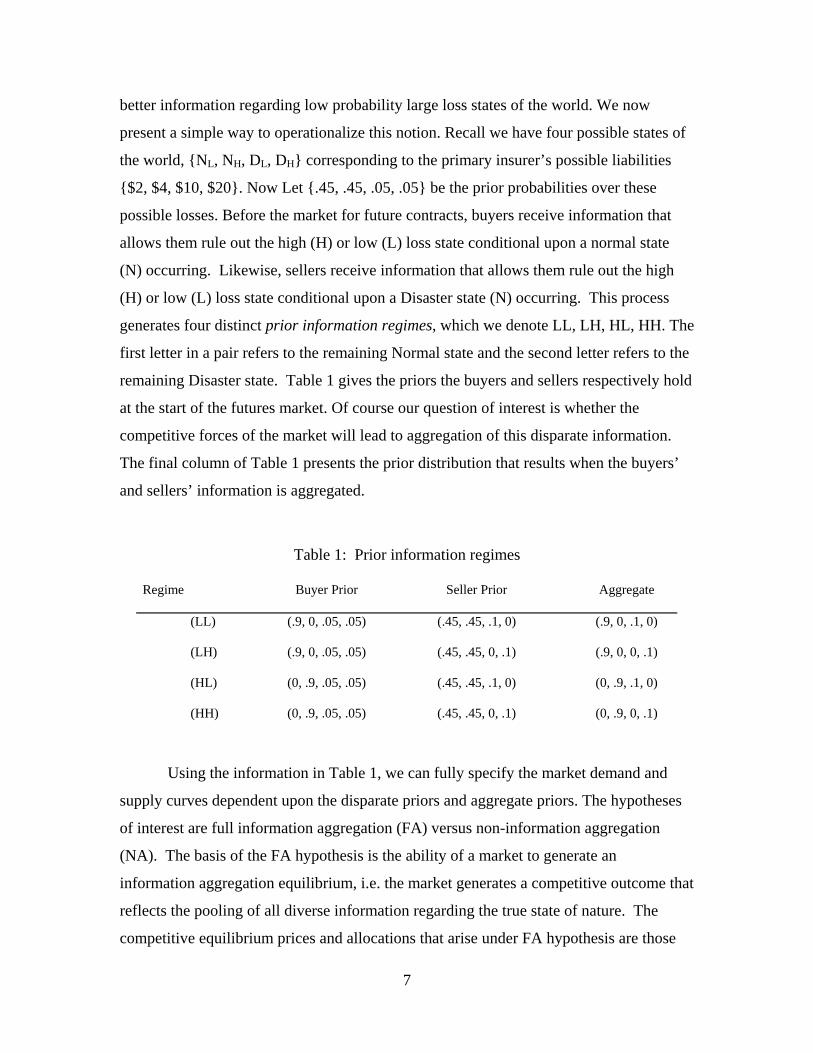
{$2, $4, $10, $20}. Now Let {.45, .45, .05, .05} be the prior probabilities over these
possible losses. Before the market for future contracts, buyers receive information that
allows them rule out the high (H) or low (L) loss state conditional upon a normal state
(N) occurring. Likewise, sellers receive information that allows them rule out the high
(H) or low (L) loss state conditional upon a Disaster state (N) occurring. This process
generates four distinct prior information regimes, which we denote LL, LH, HL, HH. The
first letter in a pair refers to the remaining Normal state and the second letter refers to the
remaining Disaster state. Table 1 gives the priors the buyers and sellers respectively hold
at the start of the futures market. Of course our question of interest is whether the
competitive forces of the market will lead to aggregation of this disparate information.
The final column of Table 1 presents the prior distribution that results when the buyers’
and sellers’ information is aggregated.
Table 1: Prior information regimes
Regime Buyer Prior Seller Prior Aggregate
(LL) (.9, 0, .05, .05) (.45, .45, .1, 0) (.9, 0, .1, 0)
(LH) (.9, 0, .05, .05) (.45, .45, 0, .1) (.9, 0, 0, .1)
(HL) (0, .9, .05, .05) (.45, .45, .1, 0) (0, .9, .1, 0)
(HH) (0, .9, .05, .05) (.45, .45, 0, .1) (0, .9, 0, .1)
Using the information in Table 1, we can fully specify the market demand and
supply curves dependent upon the disparate priors and aggregate priors. The hypotheses
of interest are full information aggregation (FA) versus non-information aggregation
(NA). The basis of the FA hypothesis is the ability of a market to generate an
information aggregation equilibrium, i.e. the market generates a competitive outcome that
reflects the pooling of all diverse information regarding the true state of nature. The
competitive equilibrium prices and allocations that arise under FA hypothesis are those
7

generated by expected demand and supply curves which use the aggregate prior to
calculate the expected dividend. The NA hypothesis is generated by the conjecture that
the market generates a competitive outcome reflecting the agents’ prior beliefs regarding
the true state of nature. The competitive equilibrium prices and allocations that arise
under the NA hypothesis are those generated by expected demand and supply curves
which use the respective priors to calculate the expected dividend.
The impact of these two competing models is generated through differing
expected dividend values. Under the FA conjecture, a competitive outcome reflects a
common expected dividend value based on the pooling of buyers’ and sellers’ private
information. The expected value is calculated as
E[d(s)] = 0.9(remaining N-state’s dividend) + 0.1(remaining D-state’s dividend).
On the other hand, if the NA conjecture holds true, the market outcome will
reflect the following distinct expected dividends for the buyer and seller;
E[d(s)]buyer = 0.9(remaining N-state’s dividend) + 0.1(average D-state’s dividend)
and
E[d(s)]seller = 0.9(average N-state’s dividend) + 0.1(remaining D-state’s dividend).
Buyers’ and Sellers’ expectations of the dividend values determine the vertical
location of supply and demand curves. Hence, the implications of the comparative statics
of FA versus NA are obtained from the inspection of the competitive equilibrium for their
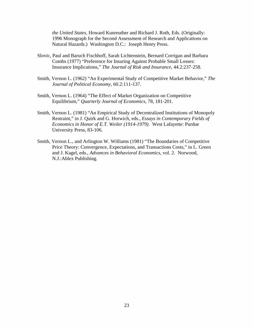
respective supply and demand curves. Table 2, and Figures 4 and 5 summarize the
equilibria for the two models in the four prior information regimes.
Table 2: Model predictions for equilibrium prices and quantities
Disaster State
Low High
LL LH
FA model: 12 units, $1.30-$1.50 12 units, $1.80-$2.00
Low
NA model: 12 units, $1.75 6 units, $1.81-$2.19
HL HH
FA model: 12 units, $2.20-$2.40 12 units, $2.70-$2.90
Normal State
High
NA model: 18 units, $2.19-$2.21 12 units, $2.25-$2.65
8
Figure 4 shows the market supply and demand curves under the FA premise for
the four prior information regimes. First, notice that for all four prior information
regimes the equilibrium market quantity is twelve units. In other words, buyers fully
reinsuring their endowed portfolio risk. Turning our attention to price, the FA outcome
generates distinct equilibrium price tunnels. The midpoints of these price tunnels
represent actuarially fair premiums for reinsurance.
In any prior information regime, the NA model will distinctly differ from the FA
model in either the equilibrium price or quantity. In the LH and HL regimes, the NA and
FA models only differ strongly in equilibrium quantities. The NA model predicts that in
the LH regime only 6 units are traded, resulting in an under-provision of reinsurance; in
the regime HL 18 units are traded, and there is an over-provision of reinsurance. One can
also observe that under prior information regimes LL and HH the equilibrium prices are
distinct under the FA and NA hypotheses, but full reinsurance is achieved in both
scenarios. However, in these two regimes the NA hypothesis does not generate actuarial
fair reinsurance premiums: In HH, the midpoint of the price tunnel is below the actuarial
fair rate and in LL the midpoint is above the actuarial fair rate.
Experimental Design
In our experiments, twelve participants are randomly partitioned into groups of
six Buyers and six Sellers. An experiment consists of a series of trading periods. In each
period, Buyers and Sellers have the opportunity to trade an asset in an oral double
auction. Before the auction starts, Buyers and Sellers are privately given information
relevant to the distribution of the dividend. After the auction, the experimenter conducts
a probability experiment that determines the actual dividend for the trading period.
Consider the time line in Figure 6. Before the start of each trading period, the
experimenter flips a coin. If the result is heads, the NL state is eliminated. If the result is
tails, the NH state is eliminated. Buyers are privately informed of the remaining Normal
state (NL or NH) with the use of a code sheet. Likewise, a second coin toss is used to
eliminate one of the Disaster states. Sellers are privately informed of the remaining
Disaster state (DL or DH).
9
Next a seven-minute open outcry double auction commences. Buyers may offer
bids or accept asks, and sellers may make asks or accept bids in an oral double auction
format. A valid bid or ask must improve upon any standing bid or ask. Once a bid or ask
is accepted, bidding starts over; buyers are then free to open bidding at any non-negative
price, and sellers are free to make an initial ask at any price between 0$ and $20. Bids,
asks, and trades are displayed on an overhead projector as they are made. After the
seven-minute trading period has expired, the final state of nature is resolved by drawing
one ball from a bingo cage in view of the participants. If the ball is numbered “1”
through “9”, the result is the remaining Normal state. If a “10” is drawn, the result is the
remaining Disaster state. The ball is returned to the bingo cage prior to the next trading
period. Buyers then receive the random values of the units they purchased and the
random transfers, and sellers pay the random costs of the units they sold.
Figure 7 below is a typical Buyer’s Decision Sheet. In row number 1 Buyer 1
carries over cumulative earnings from the previous period ($0.00 since this is the first
period). On the left side of the Buyer’s Decision sheet are four columns labeled X1, X2,
Y1, and Y2, corresponding to the state-space (NL, NH, DL, DH). In this period the
statement “not White” would inform Buyers that X1 had been eliminated, and “not Blue”
that X2 had been eliminated. There are no codes listed for the “Y” states (DL, DH), since
the buyers are not privy to this information. The values in row number 2 are net
premiums which apply in each state. Similarly, in rows three, six, nine and twelve the
values for each of the four units that Buyer number 1 may purchase are listed for each of
the four states. For each unit he purchases, Buyer 1 enters the purchase price in the
appropriate space on the far right column. After trading is finished the final state is drawn
and then completes the decision sheet. Figure 8 presents a typical Seller’s decision sheet.
Market participants are inexperienced prior to their arrival for the experiment.
They are trained in the procedure for resolving uncertainty and receiving private
information by several repetitions of the procedure without trading, and by participating
in one to three practice periods that include trading in the security.
Buyers and Sellers begin the experiment with zero cash endowments. They are
permitted to run negative cash balances without being expelled from the experiment, but
receive no compensation other than a non-salient show-up fee of five dollars if their
10

cumulative earnings are negative at the end of the experiment. The number of periods
over nine is randomly determined, and participants are not informed ahead of time which
period will be the final period.
Results and Analysis
We focus our analysis of the experimental data into two activities. First, we
compare how well the data conforms to our interior predictions for price and quantity for
the two competing models. Prices and quantities for units traded each period, with few
exceptions; do not match the equilibrium predictions for either the full-aggregation or the
no-aggregation model. Prices typically are lower than either model’s predictions and
market prices do not depend on the sellers’ prior information. The volume of reinsurance
contracts also does not reflect either model’s predictions. We do observe that the impact
of buyers’ prior information is more influential on quantity than is the sellers’ prior
information.
Since prices are generally lower than either hypothesis predicts, and buyers’ prior
information has a greater than expected impact on both price and quantity, we consider
alternative explanations. We turn to the experimental and survey research on disaster
insurance for possible explanations. Given the subjective probability biases that
underestimate the probability of disaster states found in these literatures, we explore the
possibility that the buyers’ and sellers’ posses this bias in our experiment. From the
experimental market data, we calculate implicit subjective probability beliefs of a disaster
for both buyers and sellers under the FA and NA hypotheses. The result of this exercise
suggests there is a strong bias: the buyers’ implicit beliefs are typically below the sellers’
implicit beliefs (which are on average statistically indistinguishable from 10 percent.)
Once we account for this bias, there is evidence that the NA assumption is more
appropriate. We also point out that there is an alternative to our subjective probability
bias conclusion: individuals use the objective probabilities but differ in the way they
evaluate risky choice. In this scenario we conclude that the implications of prospect
theory hold: sellers’ losses loom larger than buyers’ gains.
11
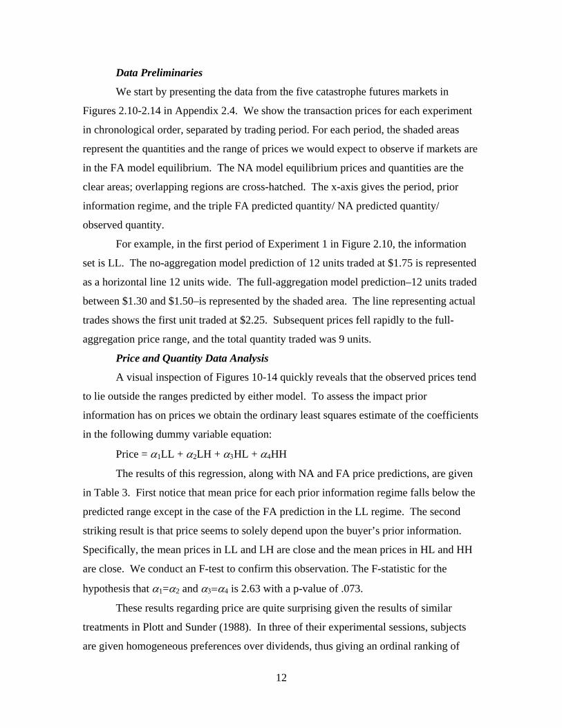
Data Preliminaries
We start by presenting the data from the five catastrophe futures markets in
Figures 2.10-2.14 in Appendix 2.4. We show the transaction prices for each experiment
in chronological order, separated by trading period. For each period, the shaded areas
represent the quantities and the range of prices we would expect to observe if markets are
in the FA model equilibrium. The NA model equilibrium prices and quantities are the
clear areas; overlapping regions are cross-hatched. The x-axis gives the period, prior
information regime, and the triple FA predicted quantity/ NA predicted quantity/
observed quantity.
For example, in the first period of Experiment 1 in Figure 2.10, the information
set is LL. The no-aggregation model prediction of 12 units traded at $1.75 is represented
as a horizontal line 12 units wide. The full-aggregation model prediction–12 units traded
between $1.30 and $1.50–is represented by the shaded area. The line representing actual
trades shows the first unit traded at $2.25. Subsequent prices fell rapidly to the full-
aggregation price range, and the total quantity traded was 9 units.
Price and Quantity Data Analysis
A visual inspection of Figures 10-14 quickly reveals that the observed prices tend
to lie outside the ranges predicted by either model. To assess the impact prior
information has on prices we obtain the ordinary least squares estimate of the coefficients
in the following dummy variable equation:
Price = α1LL + α2LH + α3HL + α4HH
The results of this regression, along with NA and FA price predictions, are given
in Table 3. First notice that mean price for each prior information regime falls below the
predicted range except in the case of the FA prediction in the LL regime. The second
striking result is that price seems to solely depend upon the buyer’s prior information.
Specifically, the mean prices in LL and LH are close and the mean prices in HL and HH
are close. We conduct an F-test to confirm this observation. The F-statistic for the
hypothesis that α1=α2 and α3=α4 is 2.63 with a p-value of .073.
These results regarding price are quite surprising given the results of similar
treatments in Plott and Sunder (1988). In three of their experimental sessions, subjects
are given homogeneous preferences over dividends, thus giving an ordinal ranking of
12
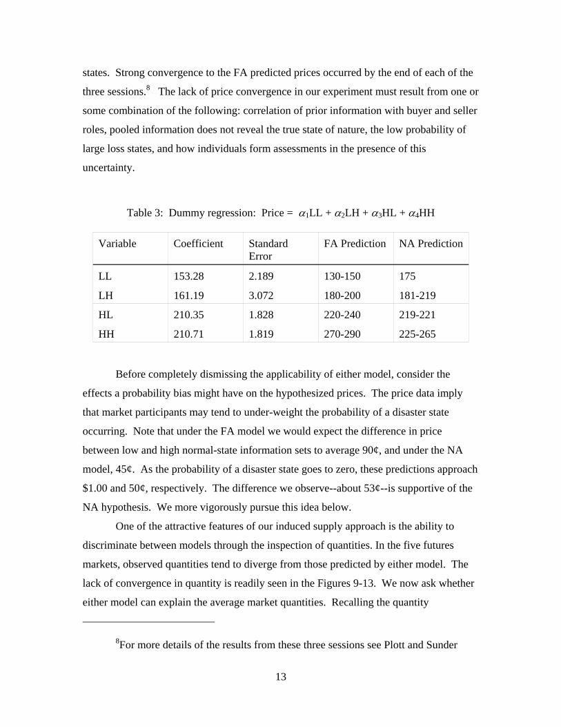
states. Strong convergence to the FA predicted prices occurred by the end of each of the
three sessions.8 The lack of price convergence in our experiment must result from one or
some combination of the following: correlation of prior information with buyer and seller
roles, pooled information does not reveal the true state of nature, the low probability of
large loss states, and how individuals form assessments in the presence of this
uncertainty.
Table 3: Dummy regression: Price = α1LL + α2LH + α3HL + α4HH
Variable Coefficient Standard Error
FA Prediction NA Prediction
LL 153.28 2.189 130-150 175
LH 161.19 3.072 180-200 181-219
HL 210.35 1.828 220-240 219-221
HH 210.71 1.819 270-290 225-265
Before completely dismissing the applicability of either model, consider the
effects a probability bias might have on the hypothesized prices. The price data imply
that market participants may tend to under-weight the probability of a disaster state
occurring. Note that under the FA model we would expect the difference in price
between low and high normal-state information sets to average 90¢, and under the NA
model, 45¢. As the probability of a disaster state goes to zero, these predictions approach
$1.00 and 50¢, respectively. The difference we observe--about 53¢--is supportive of the
NA hypothesis. We more vigorously pursue this idea below.
One of the attractive features of our induced supply approach is the ability to
discriminate between models through the inspection of quantities. In the five futures
markets, observed quantities tend to diverge from those predicted by either model. The
lack of convergence in quantity is readily seen in the Figures 9-13. We now ask whether
either model can explain the average market quantities. Recalling the quantity
8For more details of the results from these three sessions see Plott and Sunder
13

predictions of the two models summarized in Table 2, note that under the FA model we
expect 12 units to be traded in each period. Also note that under the NA model the
quantity prediction differs in two prior information regimes: in LH the quantity is six and
in HL the quantity is eighteen. The FA and NA models both give testable implications in
the following expression:
Qt = α + ν Hxt + δ xHt,
where Qt is the market quantity in period t, Hxt is dummy variable for the prior
information regimes in which buyers are informed that the low Normal state is eliminated
(i.e. regimes HL and HH), and xHt is a dummy variable for the prior information regimes
in which the seller has been informed that the low Disaster state is eliminated (i.e. LH
and HH). Under the FA model, α = 12 and ν = δ = 0 and under the NA model α = 12
and ν = - δ = 6. The OLS estimates of these coefficients are presented in Table 4. The F-
statistic for this regression (24.301) rejects the hypothesis that the mean quantity is
independent of the prior information regime. This is a rejection of the FA coupled with
symmetric subjective probability beliefs of a Disaster state. On the other hand, the
estimated model coefficients do not follow the predictions of the NA model either. The
estimated value of α (9.0) is not the predicted 12 units, and a t-test indicates a 0.00
probability that α = 12. While the estimated values of ν and δ are significantly different
from zero, and have the correct sign for the NA model, they are not equal to 6 and - 6,
respectively. The probability that ν, given an estimated value of 4.7, is equal to 6 is
0.059 and the probability that δ, given an estimated value of -1.5, is equal to - 6 is 0.000,
again according to two-sided t-tests. The other notable result of this exercise is the
magnitude of ν is significantly greater than δ. This result is indicative of the more
significant impact the buyers’ information has than the sellers’ information.
(1988) pages 1100-1102.
14

Table 4: Regression: Qt = α + ν Hxt + δ xHt
Variable Coefficient Standard Error T-Statistic
Constant 8.99 0.563 0.000
Hx 4.69 0.681 0.000
xH -1.50 0.679 0.032
In our analysis of prices we noted that observed biases were consistent with the
buyers and sellers assigning a probability of a disaster state as less than ten percent. Is
this consistent with the data on quantities? If buyers and sellers tend to under-weight the
probability of a disaster, we would still expect under the FA model a quantity of 12 units
traded in each period. Under the NA model, we would expect, as observed, a value for |δ|
less than 6; as the probability of a disaster state goes to zero, δ goes to 0 as well. As the
perceived probability of a disaster declines, however, the observed value of ν should
increase under the NA model, converging to 7 as the probability of a disaster state goes to
zero, contrary to our result. How then do we account for these results? Some possible
explanations for our results are that the experimental subjects’ perceived probability of a
disaster state changes over time, that buyers’ and sellers’ beliefs may differ, or both.
Subjective Probability Biases
We assess whether subjective probability biases combined with either the FA or
NA model can rationalize our market data. We start by assuming that the market prices
and quantities we observe each period reflect a competitive equilibrium. This assumption
relies upon the oral double auction’s substantial history of robustly generating
competitive outcomes in induced supply and demand experiments. Next we know that
the schedules of private marginal valuations and costs give us the slopes of the demand
and supply curves. What is not known is the vertical location of these curves as these are
defined by the experimental subjects’ subjective probability beliefs of a disaster state. We
further assume that all buyers have the same belief and that all sellers have the same
belief. The size of a vertical shift given a belief depends upon whether there is
information aggregation or not. We proceed by calculating implicit beliefs under both the
FA and NA hypotheses. To summarize, we have two parameters (the subjective size of
15

the supply and demand curves’ positive vertical shifts) whose values we can use to
calibrate the observed market price and quantity.
The answer to the following question is not obvious; are there role-specific
probability biases which can explain our results under these two models? To address this
question, we perform a numerical exercise in which we deduce the implicit probability
biases for buyers and for sellers using the FA and NA hypotheses. The are four main
conclusions: the NA model most plausibly explains results in most periods, buyers’
average implied beliefs of disaster under the NA hypothesis are below the actual ten
percent probability, sellers’ average probability beliefs of disaster under the NA
hypothesis do not differ significantly from ten percent on average, and correspondingly
sellers’ implied probabilities are higher than buyers’.
Let pb denote the buyers’ perceived probability of a Disaster state and ps denote
the sellers’ perceived probability of a Disaster state. Substituting into equations 1-3, we
get
E(d)buyer = (1 - pb) (remaining N-state’s dividend)
+ pb (remaining D-state’s dividend)
E(d)seller = (1 - ps) (remaining N-state’s dividend)
+ ps (remaining D-state’s dividend)
for the expected values of the common dividend under the FA hypothesis, and
E(d)buyer = (1 - pb) (remaining N-state’s dividend)
+ pb(average of the D-states’ dividends)
E(d)seller = (1 - ps) (average of the N-states’ dividends)
+ ps (remaining D-state’s dividend)
for the expected values of the common dividend under the NA hypothesis. Combining
these equations with the private value and cost increments, we solve for market
equilibrium prices and quantities for both models for all the combinations of probability
beliefs (pb, ps) over pb = 0.01, 0.02, ..., 1 and ps = 0.01, 0.02, ..., 1. From these results we
identify the range of probability beliefs of sellers and buyers in our experiments that
could support the observed quantities and median prices for each period.
The median and range of probability beliefs for buyers and sellers supporting the
observed quantities and median prices for each period’s trades are shown in
16
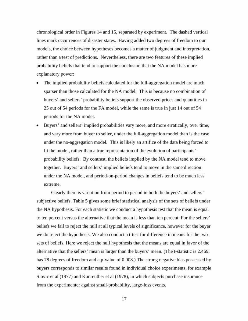
chronological order in Figures 14 and 15, separated by experiment. The dashed vertical
lines mark occurrences of disaster states. Having added two degrees of freedom to our
models, the choice between hypotheses becomes a matter of judgment and interpretation,
rather than a test of predictions. Nevertheless, there are two features of these implied
probability beliefs that tend to support the conclusion that the NA model has more
explanatory power:
• The implied probability beliefs calculated for the full-aggregation model are much
sparser than those calculated for the NA model. This is because no combination of
buyers’ and sellers’ probability beliefs support the observed prices and quantities in
25 out of 54 periods for the FA model, while the same is true in just 14 out of 54
periods for the NA model.
• Buyers’ and sellers’ implied probabilities vary more, and more erratically, over time,
and vary more from buyer to seller, under the full-aggregation model than is the case
under the no-aggregation model. This is likely an artifice of the data being forced to
fit the model, rather than a true representation of the evolution of participants’
probability beliefs. By contrast, the beliefs implied by the NA model tend to move
together. Buyers’ and sellers’ implied beliefs tend to move in the same direction
under the NA model, and period-on-period changes in beliefs tend to be much less
extreme.
Clearly there is variation from period to period in both the buyers’ and sellers’
subjective beliefs. Table 5 gives some brief statistical analysis of the sets of beliefs under
the NA hypothesis. For each statistic we conduct a hypothesis test that the mean is equal
to ten percent versus the alternative that the mean is less than ten percent. For the sellers’
beliefs we fail to reject the null at all typical levels of significance, however for the buyer
we do reject the hypothesis. We also conduct a t-test for difference in means for the two
sets of beliefs. Here we reject the null hypothesis that the means are equal in favor of the
alternative that the sellers’ mean is larger than the buyers’ mean. (The t-statistic is 2.469,
has 78 degrees of freedom and a p-value of 0.008.) The strong negative bias possessed by
buyers corresponds to similar results found in individual choice experiments, for example
Slovic et al (1977) and Kunreuther et al (1978), in which subjects purchase insurance
from the experimenter against small-probability, large-loss events.
17

Table 5: Test of mean implied probability beliefs
Statistic
Mean
Standard
Deviation
Mean Test
Statistic
P-value
Seller Belief 0.089 .062 -1.152 0.125
Buyer Belief 0.059 .046 -5.590 0.000
Our experiment is the first in which some subjects sell insurance against small-
probability, large losses. It also appears that changing the point of reference and the
framing of the reinsurance task has eliminated this bias for sellers. However, there is
another interesting perspective from which we can view these results. Instead of
assuming that individuals are expected value maximizers who have probability biases, we
could have assumed that they did not have subjective probability biases but that there
preferences differ from risk neutrality. Under this interpretation we would conclude that
the sellers give a greater assessment to the potential large losses of selling insurance
contract than buyers give to the assessment of the large gains. This interpretation is
consistent with the implications of the Kahneman and Tversky’s (1979) prospect theory
of decision making under uncertainty, where relative losses typically loom larger than
relative gains.
Conclusion
In this paper we examine an insurance market’s ability to generate equilibria
which reflect the union of market participants’ diverse information regarding the
probabilities that govern states of nature. The correlation of prior information with
market roles and the structure of uncertainty in these markets lead us to develop
significant changes to the standard experimental design, introduced by Plott and Sunder
(1988), used to test information aggregation. We found that the economic environment of
a reinsurance market failed to generate the equilibrium predictions under either the FA
model or the NA model. This is in contrast to Plott and Sunder’s finding of information
18
aggregation in simpler environments. In evaluating the hypotheses we found strong
evidence that the value of the buyer’s prior information had more impact on economic
outcomes than did the seller’s prior information. This suggested alternative explanations.
The uncertainty that characterizes insurance markets requires individuals to assess
the value of small-probability, large-loss (gain) states. A plethora of past studies show
that traditional expected utility theory’s robustness falters in these situations, and that
subjective probability biases or non-expected utility preferences can characterize
behavior. In our setting one can not distinguish between a subjective probability bias and
a utility phenomenon. After we calculate the implicit subjective probability beliefs in our
experiment we conclude that buyers posses a strong subjective probability bias and
sellers do not. The corresponding utility explanation is that sellers’ potential losses from
reinsurance contracts loom larger than buyers’ gains from reinsurance. Finally, after we
control for these decision theoretic aspects, we see that the NA hypothesis has more
explanatory power than the FA hypothesis.
These results do not provide optimism that insurance markets, such as the
catastrophe futures index introduced by the CBOT in 1992, can lead to outcomes in
which information is aggregated and risk is efficiently shared. Given the strong
desirability of the information aggregation property in an insurance market, it is
worthwhile to explore whether other financial instruments (e.g. PCS option spreads and
Act of God Bonds) and other institutions (such as the long standing bilateral contractual
relationships that governed the reinsurance market prior to 1990) fare better than the
market we study here.
Our results also suggest future directions in the study of information aggregation
in general. Specifically, can we explain why the challenging decision making under
uncertainty environment of catastrophe insurance impedes the information aggregation
process? If we can not answer this question, can we at least establish the boundary of this
breakdown empirically? Furthermore, in previous experiments in which information
aggregation occurs, the pooled information reveals the true state. In our experiments
pooled information does not reveal the true state of nature, and it is of interest to assess
the impact this has. Clearly, in most cases of interest, pooled information does not reveal
the true state. Finally, we believe the introduction of the induced supply and demand
19

approach to the study of markets with uncertainty is an innovation which may permit the
performance of a wider class of experiments. The robustness of this approach needs to be
more thoroughly tested.
20

Bibliography
Cox, Samuel H. and Robert G. Schwebach (1992) “Insurance Futures and Hedging Insurance Price Risk,” The Journal of Risk and Insurance, 59.4:628-644.
Cummins, J. David and Hélyette Geman (1995) “Pricing Catastrophe Insurance Futures
and Call Spreads: An Arbitrage Approach,” The Journal of Fixed Income, 4:46-57.
D’Arcy, Stephen P. and Virgina G. France (1992) “Catastrophe Futures: A Better Hedge
for Insurers,” The Journal of Risk and Insurance, 59.4:575-601. Doherty, Neil A. (1996) “Insurance Markets and Climate Change,” Presented at IIASA
1996 conference Climate Change: Cataclysmic Risk and Fairness. Doherty, Neil A. (1997) “Innovations in Managing Catastrophe Risk,” Journal of Risk
and Insurance, 64.4:713-718. Forsythe, Robert and Russell Lundholm (1990) “Information Aggregation in an
Experimental Market,” Econometrica, 58.2:309-347. Gjerstad, Steven and Jason Shachat (1996) “A General Equilibrium Structure for Induced
Supply and Demand,” UCSD Economics Discussion Paper 96-35. Harrington, Scott E., Steven V. Mann and Greg Niehaus (1995) “Insurer Capital
Structure Decisions and the Viability of Insurance Derivatives,” The Journal of Risk and Insurance, 62.3:483-508.
Harrington, Scott and Greg Niehaus (1999) “Basis Risk with PCS Catastrophe Insurance
Derivative Contracts,” Journal of Risk and Insurance, 66:49-82. Holt, Charles A., Loren Langan, and Anne P. Villamil (1986) “Market Power in Oral
Double Auctions,” Economic Inquiry, 24, 107-123. Kahneman, Daniel and Amos Tversky (1979) “Prospect Theory: An Analysis of Decision
Under Risk,” Econometrica 47:263-291. Kunreuther, Howard (1996) “Mitigating Losses and Providing Protection against
Catastrophic Risks: The Role of Insurance and Other Policy Instruments,” The Geneva Lecture, presented at the European Society for Risk Analysis, June 4, 1996, Guilford, England.
Kunreuther, Howard (1998) “Preface,” in Paying the Price: The Status and Role of
Insurance Against Natural Disasters in the United States, Howard Kunreuther and Richard J. Roth, Eds. (Originally: 1996 Monograph for the Second
21
Assessment of Research and Applications on Natural Hazards.) Washington D.C.: Joseph Henry Press.
Kunreuther, Howard, Ralph Ginsberg, Louis Miller, Philip Sagi, Paul Slovic, Bradley
Borkan and Norman Katz (1978) Disaster Insurance Protection: Public Policy Lessons, John Whiley and Sons: New York.
Lecomte, Eugene (1996) “Hurricane Insurance Protection in Florida,” chapter 5 in in
Paying the Price: The Status and Role of Insurance Against Natural Disasters in the United States, Howard Kunreuther and Richard J. Roth, Eds. (Originally: 1996 Monograph for the Second Assessment of Research and Applications on Natural Hazards.) Washington D.C.: Joseph Henry Press.
Marlett, David C. and Alan Eastman (1997) “The Estimated Impact of Residual Market
Assessments on Florida Property Insurers,” American Risk and Insurance Association 1997 Annual Meeting.
McClelland, Gary H., William D. Schulze and Don Coursey (1993) “Insurance for Low-
Probability Hazards: A Bimodal Response to Unlikely Events,” Journal of Risk and Uncertainty, 7:95-116.
Niehaus, Greg and Steven V. Mann (1992) “The Trading of Underwriting Risk: An
Analysis of Insurance Futures Contracts and Reinsurance,” The Journal of Risk and Insurance, 59.4:601-627.
Nutter, Franklin W. (1994) “The Role of Government in the United States in Addressing
Natural Catastrophes and Environmental Exposures,” The Geneva Papers on Risk and Insurance: Issues and Practice, (no. 72) 19:244-256.
Ohare, Dean (1994) “The Need for Insurers to Change,” Geneva Papers on Risk and
Insurance: Issues and Practice, (no. 72) 19:357-364. Plott, Charles R. and Shyam Sunder (1982) “Efficiency and Experimental Security
Markets with Insider Information: An Application of Rational Expectations Models,” Journal of Political Economy, 90:663-698.
Plott, Charles R. and Shyam Sunder (1988) “Rational Expectations and the Aggregation
of Diverse Information in Laboratory Security Markets,” Econometrica, 56.5:1085-1118.
Plott, Charles R., Jorgen Wit, and Winston C. Yang (2003) “Parimutuel betting markets
as information aggregation devices: experimental results,” Economi Theory, 22.2:311-351.
Roth, Richard J. Jr. (1996) “Earthquake Insurance Protection in California,” chapter 4 in
Paying the Price: The Status and Role of Insurance Against Natural Disasters in
22
the United States, Howard Kunreuther and Richard J. Roth, Eds. (Originally: 1996 Monograph for the Second Assessment of Research and Applications on Natural Hazards.) Washington D.C.: Joseph Henry Press.
Slovic, Paul and Baruch Fischhoff, Sarah Lichtenstein, Bernard Corrigan and Barbara
Combs (1977) “Preference for Insuring Against Probable Small Losses: Insurance Implications,” The Journal of Risk and Insurance, 44.2:237-258.
Smith, Vernon L. (1962) “An Experimental Study of Competitive Market Behavior,” The
Journal of Political Economy, 60.2:111-137. Smith, Vernon L. (1964) “The Effect of Market Organization on Competitive
Equilibrium,” Quarterly Journal of Economics, 78, 181-201. Smith, Vernon L. (1981) “An Empirical Study of Decentralized Institutions of Monopoly
Restraint,” in J. Quirk and G. Horwich, eds., Essays in Contemporary Fields of Economics in Honor of E.T. Weiler (1914-1979). West Lafayette: Purdue University Press, 83-106.
Smith, Vernon L., and Arlington W. Williams (1981) “The Boundaries of Competitive
Price Theory: Convergence, Expectations, and Transactions Costs,” in L. Green and J. Kagel, eds., Advances in Behavioral Economics, vol. 2. Norwood, N.J.:Ablex Publishing.
23

loss size
prob
abilit
y de
nsity
Buyer's Information Seller's Information
Figure 1: Reinsurance market risk and information structure
0
4
8
12
16
20
0 1 2 3 4 5
Contracts
Pric
e
State DL
State NH
State NL
State DH
Figure 2: A Primary Insurer’s State Dependent Demand Functions for Future Contracts
24

0
4
8
12
16
20
0 1 2 3 4 5
Contracts
Pric
e
State DL
State NH
State NL
State DH
Figure 3: A Reinsurer’s State Dependent Supply Functions for Future Contracts
Figure 4: Full-aggregation equilibrium induced supply and demand
25
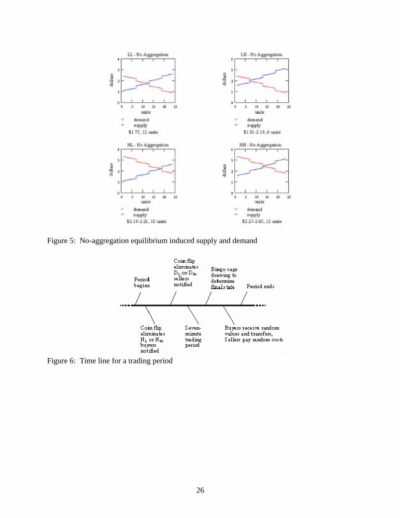
Figure 5: No-aggregation equilibrium induced supply and demand
Figure 6: Time line for a trading period
26

Figure 4. Buyer’s Decision Sheet
1Period:1Buyer Decision Sheet for Buyer #
Name:
Probability of an X-state: 90%
Probability of a Y-state: 10%
Row #Unit # State
0.00Cumulative Earnings1Y2Y1X2X1 — — Blue White
Random Transfer2****-5.400.602.60
Unit Value3110.545.542.541.54
Purchasing Price4
Unit Earnings (3 - 4)5
Unit Value6210.305.302.301.30
Purchasing Price7
Unit Earnings (6 - 7)8
Unit Value939.664.661.660.66
Purchasing Price10
Unit Earnings (9 - 10)11
Unit Value1249.424.421.420.42
Purchasing Price13
Unit Earnings (12 - 13)14
Total Unit Earning s 15
(5+8+11+14)
Period Net Earning s 16
(2 + 15)
Cumulative Earnings 17
(1 + 16)
27
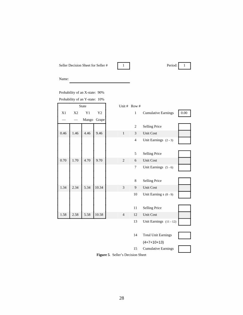
Figure 5. Seller’s Decision Sheet
1Period:1Seller Decision Sheet for Seller #
Name:
Probability of an X-state: 90%
Probability of an Y-state: 10%
Row #Unit # State
0.00Cumulative Earnings1Y2Y1X2X1
Grape Mango — —
Selling Price2
Unit Cost319.464.461.460.46
Unit Earnings (2 - 3)4
Selling Price5
Unit Cost629.704.701.700.70
Unit Earnings (5 - 6)7
Selling Price8
Unit Cost9310.345.342.341.34
Unit Earning s (8 - 9)10
Selling Price11
Unit Cost12410.585.582.581.58
Unit Earnings (11 - 12)13
Total Unit Earnings 14
(4+7+10+13)
Cumulative Earnings 15
28

Figure 9: Market 1
Figure 10: Market 2
29

Figure 11: Market 3
Figure 12: Market 4
30
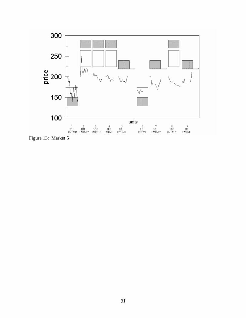
Figure 13: Market 5
31
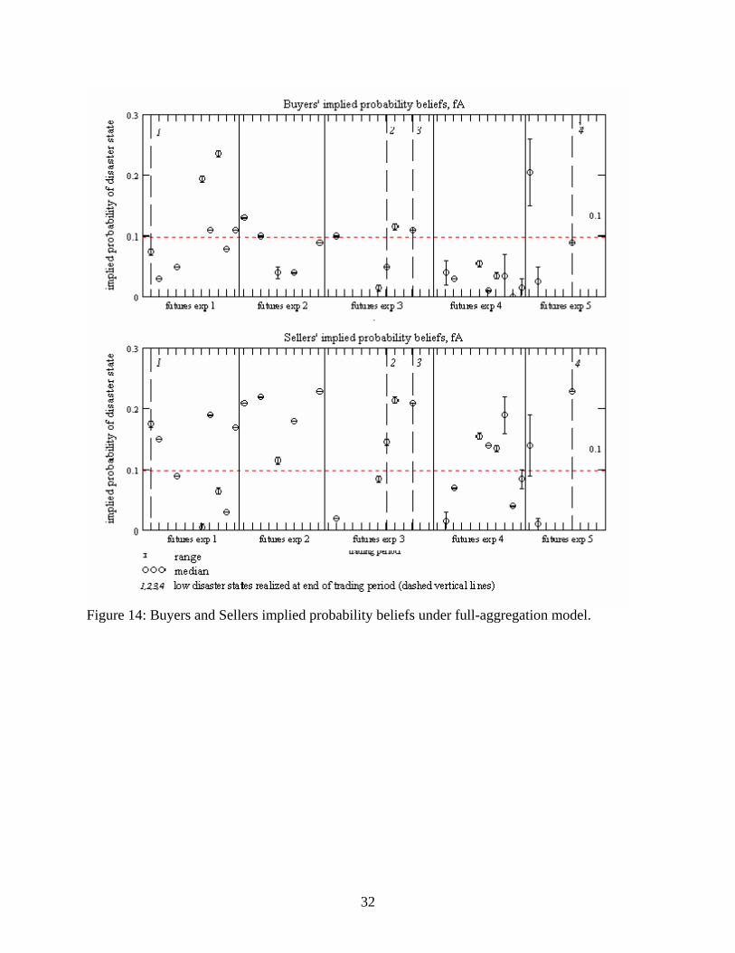
Figure 14: Buyers and Sellers implied probability beliefs under full-aggregation model.
32
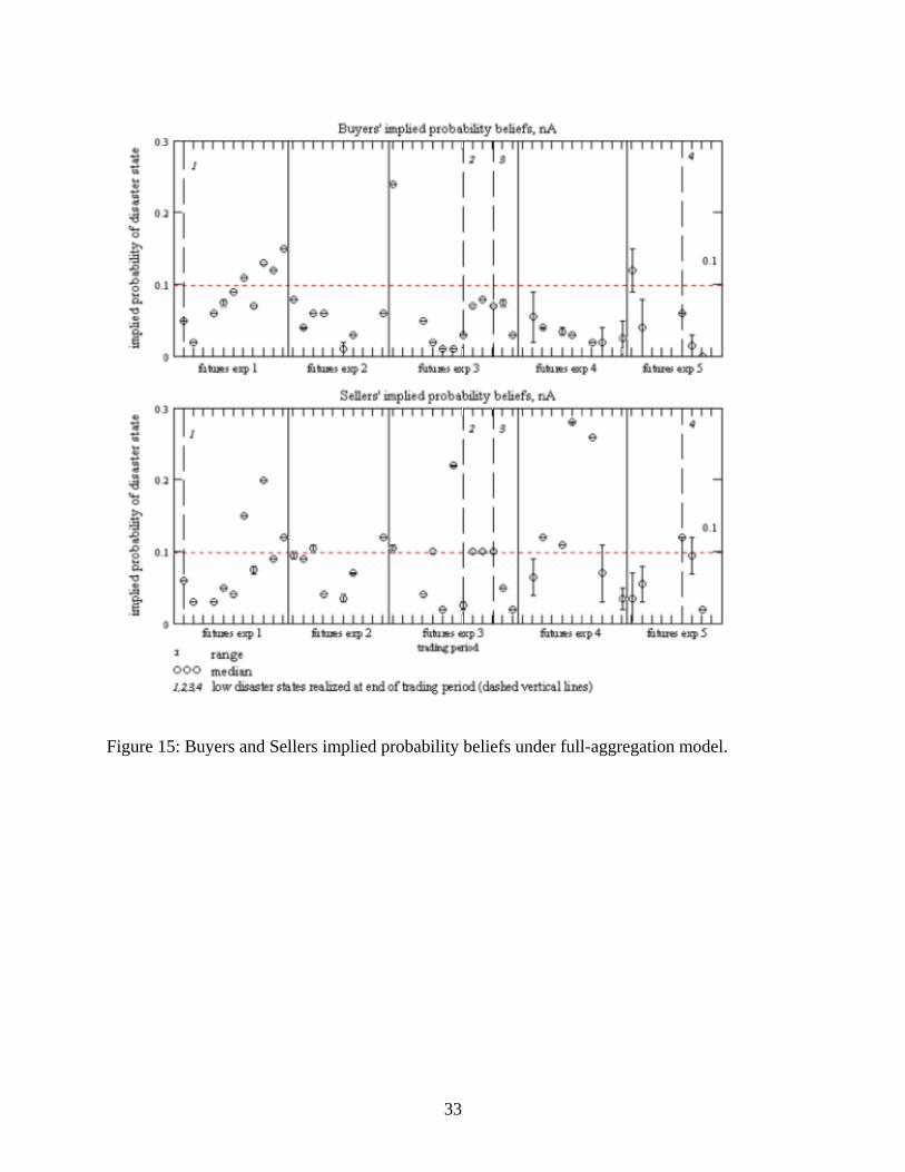
Figure 15: Buyers and Sellers implied probability beliefs under full-aggregation model.
33