influence of surface height variance on distribution of ground control

Influence of surface height varianceon distribution of ground controlpoints

Sudniran PhetcharatMasahiko NagaiTaravudh Tipdecho

Downloaded From: https://www.spiedigitallibrary.org/journals/Journal-of-Applied-Remote-Sensing on 07 Feb 2022Terms of Use: https://www.spiedigitallibrary.org/terms-of-use

Influence of surface height variance on distributionof ground control points

Sudniran Phetcharat, Masahiko Nagai, and Taravudh TipdechoAsian Institute of Technology, School of Engineering and Technology,Remote Sensing and Geographic Information Systems, P.O. Box 4,

Klong Luang, Pathumthani 12120, [email protected]

Abstract. The process of geometric correction of a satellite image requires a network of groundcontrol points (GCPs), the density of which depends on the accuracy required. In this study, anapproach to determine the distribution of the GCPs was developed based on dividing the surfaceterrain into zones of low- and high-height variances. Comparative statistics were investigated tosummarize the optimum number and distribution of the GCPs. For a uniform arrangement of 10GCPs, the accuracy using root mean square error was 7.19 m. This accuracy was improved to6.13 m following the inclusion of just two additional GCPs in the zone of high-surface heightvariance. Thus, the transformation using the polynomial model and a set of GCPs, for which thesurface variance in height was considered, resulted in greater accuracy than using the conven-tional uniformly distributed method. In addition, the time required for the trial-and-error selec-tion of the locations of the GCPs was reduced. Our results suggest that a method that considersthe variance in height of the surface terrain could be applied to various types of images such assatellite or aerial photography. © The Authors. Published by SPIE under a Creative CommonsAttribution 3.0 Unported License. Distribution or reproduction of this work in whole or in part requiresfull attribution of the original publication, including its DOI. [DOI: 10.1117/1.JRS.8.083684]

Keywords: surface variance in height; ground control points; polynomial coefficients function.

Paper 13118 received Apr. 11, 2013; revised manuscript received Dec. 5, 2013; accepted forpublication Dec. 31, 2013; published online Jan. 29, 2014.

1 Introduction

Aerial photographs and satellite images are fundamental sources of data used for the analysis ingeographic information systems, remote sensing, and mapping. The image acquisition processdepends on the type of sensor used. Geometric distortion of the images from current pushbroomsatellites, such as SPOT, ASTER, and Quickbird, is derived from two principal sources: inac-curate modeling of the charge-coupled device sensor geometry and small movements of theinstrument platform during image acquisition.1 High-resolution satellite images are prone to geo-metric distortion and thus, geometric correction is desirable.2 The primary distortions have bothinternal and external sources. The former are the distortions inherent within a system that can beadjusted based on the characteristics of the sensor, e.g., lens distortion, which can be compen-sated for using the colinearity equation. The latter are the errors introduced from sources such asthe Earth’s curvature and changes in atmospheric conditions, the reflective properties of light,and surface topography. These external sources distort the image directly, causing positionswithin the image to be inconsistent with those on the ground. Variations in elevation and surfaceroughness cause a particular type of distortion known as perspective distortion, which normallyhappens when using a short focal length.

In some cases, images used in satellite data analysis have no accompanying informationregarding the sensor model of the satellite and thus, they may require adjustment usingother appropriate models. Different methods for the transformation of one coordinate systemto another have been proposed,3 e.g., the Helmert transformation, affine transformation,pseudo-affine transformation, projective transformation, second-order conformal transforma-tion, and polynomial transformation. Of these, the polynomial model is simple and easy touse. Historically, polynomial models are among those empirical models used most frequently

Journal of Applied Remote Sensing 083684-1 Vol. 8, 2014


http://dx.doi.org/10.1117/1.JRS.8.083684





for fitting functions.4 The distortion is predominantly low frequency and therefore, it can bemodeled using a low-order polynomial. Polynomials offer many advantages such as simpleform, moderate flexibility of shapes, well-known and understood properties, and ease of usecomputationally. This model transforms three-dimensional (3-D) object coordinates to imagecoordinates and converts the data from 3D to two-dimensional (2-D). This transformationrequires the use of ground control points (GCPs), which may be obtained using integrated infor-mation from ground surveys, photogrammetry, or GPS data comprising x, y, and z coordinates.Rizos and Satirapod5 stated that the differential GPS technique generally provides an accuracy ofbetter than 3 m in the horizontal component at twice the distance root mean square error (RMSE)(at approximately 95% confidence level). The results of the transformation are the coefficients ofthe polynomial equation.

Generally, GCPs for geometric correction are distributed uniformly throughout the entireimage using a square grid.6 This approach is suitable for the calculation and determinationof the GCP positions, but it does not account for onsite topography. The number of GCPs shouldbe higher in mountainous areas or in areas with high variance of surface height. However,obtaining GCPs by field survey or other methods can be costly and time consuming; therefore,the optimization of the GCP network is desirable. The GCP locations should have high-spatialfrequency and well-defined positions such as at river crossings and road junctions.7 Elevation isone of the three important variables needed to determine the coefficients of the 3-D polynomialequation and the positions of the GCPs. The GCPs should be located to sample the 3-D contentof the data, i.e., a greater number of samples in regions of high height variation. Wang et al.stated that the spatial distribution of GCPs may affect the accuracy and quality of image cor-rection.8 This study aims to determine the optimum number of GCPs required for each type ofsurface by classifying the level of height variance based on the standard deviation (SD) of theelevation distribution.

2 Study Area and GCP Availability

The study area is located in Chiang Mai and Lampoon, which are northern provinces ofThailand, approximately 600 km from Bangkok. This area has a variety of topographic char-acteristics including both flat areas and highly complex surfaces. The coordinates of the upperleft and lower right corners of the target area are 98.83040° E, 18.7702° N and 99.02550° E,18.5918° N, respectively, encompassing an area of approximately 406 km2. The observed sur-face variance in height, based on a digital elevation model (DEM), is highly diverse, causing highvalues of SD and difference in elevation (the highest – the lowest), which are 69 and 643 m,respectively. Areas with high variance in height (mountainous terrain) accounted for ∼35% ofthe area, mainly to the northwest; and the remaining 65% in eastern and southern parts of theimage was areas with low variance in height (urban). Figure 1 shows an image of the landscapeof this area acquired from Worldview-1 (Level 1B) on February 23, 2008. Level 1B data are

Fig. 1 Study area in Chiang Mai and Lampoon, Thailand.

Phetcharat, Nagai, and Tipdecho: Influence of surface height variance on distribution of ground control points



radiometric-corrected, sensor-corrected, and band-aligned, providing imagery as seen fromthe spacecraft without any further correction of terrain distortion. Worldview-1 operates atan altitude of 496 km with a resolution of 50 cm in the panchromatic band at nadir. The specifiedgeolocation accuracy of the instrument is less than 4.0 m CE90 (Circular Error of 90%) withoutGCPs in a 2-D image.9

There are 78 GCP points with 3-D coordinates and accuracy of 0.2 m available for the image,which are provided by the Land Development Department of Thailand; however, only 68 GCPpoints were used in this study as independent check points (ICPs). The ICPs are those points thathave been used in the RMSE process for checking the transformed image. A static and kinematicGPS survey was used to acquire the positions of the GCPs. All GCPs including the ICPs areshown in Fig. 2.

3 Three-Dimensional Polynomial Model

Using GCPs to determine the coefficients, polynomial modeling is applied to generate a newsurface model with enhanced accuracy, both in terms of shape and position of the image.Stability analysis of the polynomial differential equations is a central topic in nonlinear dynamicsand control, which in recent years has undergone major algorithmic developments followingadvances in optimization theory.10 The transformation model creates a new geocoded imagespace, in which interpolated pixel values will be placed later during resampling. The procedurerequires that the polynomial equations to be fitted to the GCPs using least squares criteria tomodel the geometrical distortion in the image domain independently of its source. The degree ofthe polynomial may be chosen based on the desired accuracy and the number of GCPs available.In general, polynomial equations used for modifying images are typically second or third order.The independent variables in the equation are Xn, Yn, and Zn. The dependent variables arethe row and column positions of the pixel (rp and cp).

For matching the point of the GCP chip on the ground and the associated point on the dis-torted image, the surrounding observation has been used. The coordinate functions are as shownbelow:

rp ¼ pvðXn; Yn; ZnÞ (1)

cp ¼ phðXn; Yn; ZnÞ; (2)

where rp is the position of the pixel in the row that corresponds to the column of the pixel inthe distorted satellite image, cp is the position of the pixel in the column that correspondsto the row of the pixel in the distorted satellite image, and X, Y, Z, and n are the ground

Fig. 2 All GCPs and ICPs across the digital elevation model (DEM).




coordinates that correspond to the east and north positions, elevation, and local position number,respectively.

Function pvðXn; Yn; ZnÞ and phðXn; Yn; ZnÞ, as a second-order polynomial, can be generatedfrom Eqs. (1) and (2) as follows:

rp ¼ a0 þ a1Xn þ a2Yn þ a3Zn þ a4XnYn þ a5XnZn þ a6YnZn þ a7X2n þ a8Y2

n þ a9Z2n: (3)

cp ¼ b0 þ b1Xn þ b2Yn þ b3Zn þ b4XnYn þ b5XnZn þ b6YnZn þ b7X2n þ b8Y2

n þ b9Z2n: (4)

Generally, polynomial transformations with terms up to the first order can model rotation,scale, and translation and are computationally economical. As additional terms are added, morecomplex warping can be achieved. aj and bj ðj ¼ 0; 1; : : : ; 9Þ are coefficients that are unknownbut can be calculated using the least squares method from the error E of all data n deviating fromthe function pðXn; Yn; ZnÞ as follows:

E ¼Xni¼1

½rp − ða0 þ a1Xi þ a2Yi þ : : : þ a9Z2i Þ�2: (5)

Then, the minimum error can be found by differentiating Ewith respect to the coefficient andsetting the result to zero; thus, the following 10 subequations are produced:

∂E∂a0

¼ 0;∂E∂a1

¼ 0;∂E∂a2

¼ 0; : : : ;∂E∂a9

¼ 0: (6)

The results of these equations will be in the form of a matrix with the following equation:2666666664

nP

ni¼1 Xi

Pni¼1 Yi · · ·

Pni¼1 Z

2iP

ni¼1 Xi

Pni¼1 X

2i

Pni¼1 XiYi · · ·

Pni¼1 XiZ2

iPni¼1 Yi

Pni¼1 XiYi

Pni¼1 Y

2i · · ·

Pni¼1 YiZ2

i

..

. ... ..

.· · · ..

.

Pni¼1 Z

2i

Pni¼1 XiZ2

i

Pni¼1 YiZ2

i. .. P

ni¼1 Z

4i

3777777775

2666666664

a0a1a2

..

.

a9

3777777775

2666666664

Pni¼1 rpP

ni¼1 XirpPni¼1 Yirp

..

.

Pni¼1 Z

2i rp

3777777775: (7)

On the left side of this equation, a symmetric matrix “A” represents the known values squarematrix (10 × 10), and matrix “B” denotes the coefficients matrix (10 × 1). On the right side,matrix “C” represents the known value matrix (10 × 1). Therefore, the multiplication of bothsides of Eq. (7) with inverse matrix A provides the coefficients a0; a1; a2; : : : ; a9.

4 Surface Variance in Height Classification Method

Bayer et al.11 stated that the synthetic aperture radar images reveal radiometric image distortionsthat are caused by terrain undulations, because the 3-D nature of the surface is ignored and GCPsare distributed uniformly here. We account for this and increase the sampling density dependingon local variations of elevation. Here, two zones were chosen for these data; however, this maynot be optimal. One method to allow for this would be to partition the image into several regionsbased on height variation and to have different GCP densities in the different regions. Manyhistogram-based approaches identify a threshold for the binarization of an image by approxi-mating a histogram as two distribution functions.12–14 Wu et al. proposed procedures for change-point detection (threshold selection) by determining the maximum distance from a line L to acumulative histogram, where line L connects the first and last points of the cumulative histogram(Fig. 3).15 The main advantage of this method is being able to use the height to find a change-point of the surface variance in height. It is also appropriate for a large number of data points.

In Fig. 3, the straight line L connecting ðx1; y1Þ and ðxN; yNÞ is a cumulative “equalized”histogram. Histogram equalization modifies the pixel values in such a way that the intensity




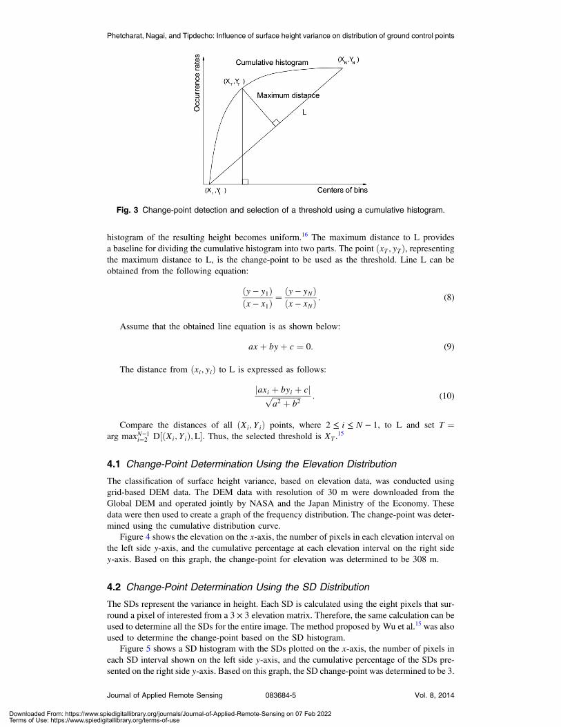
histogram of the resulting height becomes uniform.16 The maximum distance to L providesa baseline for dividing the cumulative histogram into two parts. The point ðxT; yTÞ, representingthe maximum distance to L, is the change-point to be used as the threshold. Line L can beobtained from the following equation:

ðy − y1Þðx − x1Þ

¼ ðy − yNÞðx − xNÞ

: (8)

Assume that the obtained line equation is as shown below:

axþ byþ c ¼ 0: (9)

The distance from ðxi; yiÞ to L is expressed as follows:

jaxi þ byi þ cjffiffiffiffiffiffiffiffiffiffiffiffiffiffiffia2 þ b2

p : (10)

Compare the distances of all ðXi; YiÞ points, where 2 ≤ i ≤ N − 1, to L and set T ¼arg maxN−1

i¼2 D½ðXi; YiÞ;L�. Thus, the selected threshold is XT .15

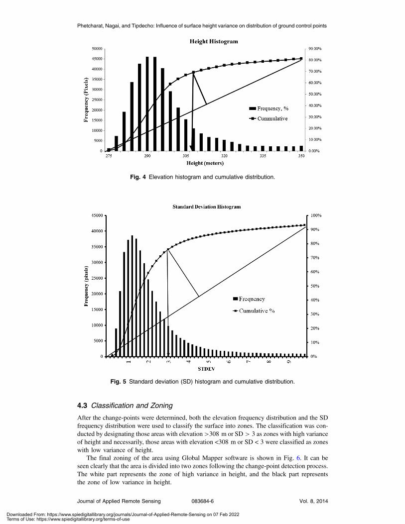
4.1 Change-Point Determination Using the Elevation Distribution

The classification of surface height variance, based on elevation data, was conducted usinggrid-based DEM data. The DEM data with resolution of 30 m were downloaded from theGlobal DEM and operated jointly by NASA and the Japan Ministry of the Economy. Thesedata were then used to create a graph of the frequency distribution. The change-point was deter-mined using the cumulative distribution curve.

Figure 4 shows the elevation on the x-axis, the number of pixels in each elevation interval onthe left side y-axis, and the cumulative percentage at each elevation interval on the right sidey-axis. Based on this graph, the change-point for elevation was determined to be 308 m.

4.2 Change-Point Determination Using the SD Distribution

The SDs represent the variance in height. Each SD is calculated using the eight pixels that sur-round a pixel of interested from a 3 × 3 elevation matrix. Therefore, the same calculation can beused to determine all the SDs for the entire image. The method proposed by Wu et al.15 was alsoused to determine the change-point based on the SD histogram.

Figure 5 shows a SD histogram with the SDs plotted on the x-axis, the number of pixels ineach SD interval shown on the left side y-axis, and the cumulative percentage of the SDs pre-sented on the right side y-axis. Based on this graph, the SD change-point was determined to be 3.

Fig. 3 Change-point detection and selection of a threshold using a cumulative histogram.




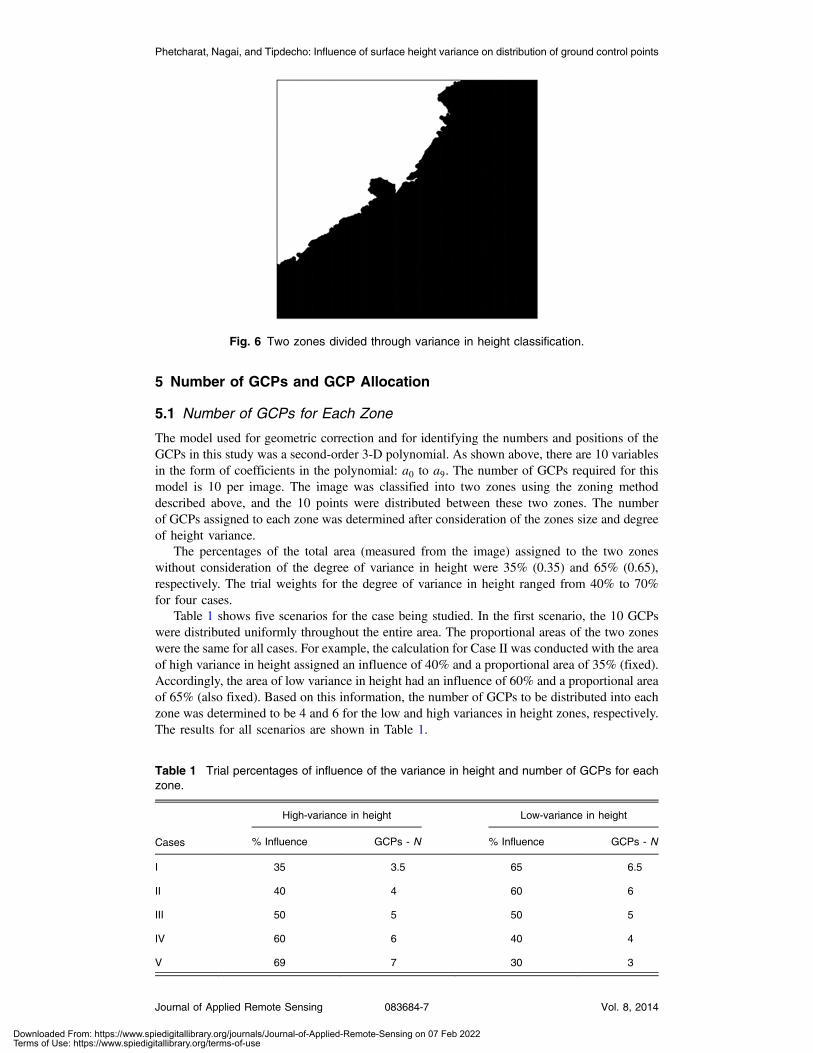
4.3 Classification and Zoning

After the change-points were determined, both the elevation frequency distribution and the SDfrequency distribution were used to classify the surface into zones. The classification was con-ducted by designating those areas with elevation >308 m or SD > 3 as zones with high varianceof height and necessarily, those areas with elevation <308 m or SD < 3 were classified as zoneswith low variance of height.

The final zoning of the area using Global Mapper software is shown in Fig. 6. It can beseen clearly that the area is divided into two zones following the change-point detection process.The white part represents the zone of high variance in height, and the black part representsthe zone of low variance in height.

Fig. 4 Elevation histogram and cumulative distribution.

Fig. 5 Standard deviation (SD) histogram and cumulative distribution.




5 Number of GCPs and GCP Allocation

5.1 Number of GCPs for Each Zone

The model used for geometric correction and for identifying the numbers and positions of theGCPs in this study was a second-order 3-D polynomial. As shown above, there are 10 variablesin the form of coefficients in the polynomial: a0 to a9. The number of GCPs required for thismodel is 10 per image. The image was classified into two zones using the zoning methoddescribed above, and the 10 points were distributed between these two zones. The numberof GCPs assigned to each zone was determined after consideration of the zones size and degreeof height variance.

The percentages of the total area (measured from the image) assigned to the two zoneswithout consideration of the degree of variance in height were 35% (0.35) and 65% (0.65),respectively. The trial weights for the degree of variance in height ranged from 40% to 70%for four cases.

Table 1 shows five scenarios for the case being studied. In the first scenario, the 10 GCPswere distributed uniformly throughout the entire area. The proportional areas of the two zoneswere the same for all cases. For example, the calculation for Case II was conducted with the areaof high variance in height assigned an influence of 40% and a proportional area of 35% (fixed).Accordingly, the area of low variance in height had an influence of 60% and a proportional areaof 65% (also fixed). Based on this information, the number of GCPs to be distributed into eachzone was determined to be 4 and 6 for the low and high variances in height zones, respectively.The results for all scenarios are shown in Table 1.

Fig. 6 Two zones divided through variance in height classification.

Table 1 Trial percentages of influence of the variance in height and number of GCPs for eachzone.

Cases

High-variance in height Low-variance in height

% Influence GCPs - N % Influence GCPs - N

I 35 3.5 65 6.5

II 40 4 60 6

III 50 5 50 5

IV 60 6 40 4

V 69 7 30 3




5.2 GCP Allocation

In general, GCPs are used in uniform distribution patterns. Points should first be placed onthe four corners of the image to control the accuracy of regional mapping.17 Then, the otherGCPs should be distributed uniformly within each zone. In this study, the selection of the loca-tions of the GCPs was conducted manually. The locations of the GCPs for the five trial cases,based on the numbers of GCPs presented in Table 1, are shown in Fig. 7.

Figure 7(a) shows Case I, in which the GCPs were allocated using the uniform distributionmethod. Four GCPs were placed at the corners to control the boundaries of the study area.The fifth GCP was placed at the center of the area, and the remaining five GCPs were spacedequally around the fifth point, resulting in a pentagon shape. The variance in height was notconsidered in this case.

For Cases II to V presented in Figs. 7(b) to 7(e), the GCP allocation based on a uniformdistribution was conducted as follows:

1. Ten assumed points were defined within the study area, corresponding to the coefficientsin the polynomial (a0 to a9), and each point is circled to show clearly the definitionapplied in each trial case.

2. First, four GCPs were allocated near the four corners of the image.3. The other priority GCPs should be allocated to the corners of each zone.4. Then, an available GCP is selected as close as possible to the center of each

assumed point.5. The remaining GCPs should be allocated in other areas within the same zone for

an equidistant coverage.

6 Results and Evaluation of Accuracy

The evaluation of accuracy was conducted by cross-checking the GCP positions on the trans-formed image in 2-D ðXest; YestÞ against the actual locations at the same positions on the groundin 2-D ðXact; YactÞ. The ground coordinates for the transformed image can be expressed byreversing Eqs. (3) and (4), because the polynomial transformation can be reversed from objectcoordinates to image coordinates, or vice versa. The accuracy of the transformation wasdetermined using the RMSE with all the remaining 68 ICPs scattered throughout the image.The equation used in this calculation was as follows:18

Fig. 7 GCP allocation for each trial case: (a) I—uniformly distributed, (b) II, (c) III, (d) IV, and (e) V.




RMSE ¼ffiffiffiffiffiffiffiffiffiffiffiffiffiffiffiffiffiffiffiffiffiffiffiffiffiffiffiffiffiffiffiffiffiffiffiffiffiffiffiffiffiffiffiffiffiffiffiffiffiffiffiffiffiffiffiffiffiffiffiffiffiffiffiffiffiffiffiffiffiffiffiffiffiffiffiffiffiffiffiffiffiffiffiffiffiffiffiffiffiffiffiffiffi��P

ni¼1 ðXact − XestÞ2

�þ �Pni¼1 ðYact − YestÞ2

��n

s; (11)

where n is the number of all remaining ICPs, Xact and Yact are the actual control points’ X and Ycoordinates, and Xest and Yest are the estimated control points’ X and Y coordinates.

Table 2 shows the RMSEs results when the GCP distribution was selected by varying thenumbers and locations of the GCPs. It can be concluded that Case I is the best case because itshows the lowest average RMSE. This is probably because Case I applied a uniform distribution,which is a popular method for allocating GCPs. Furthermore, the variance in height of the sur-face in this case was ignored. The other cases that resulted in an increasing RMSE after the GCPpositions were moved from the area of low variance in height to the area with high variance inheight.

To compare the 68 points in the transformed image, 68 ICPs were used and the evaluateddirection of error, both in the x- and y-axes, is presented in Fig. 8. It was necessary to enlargethe scale by a factor of 100 to show clearly the direction of error. Furthermore, Fig. 8 shows thatthere were still errors in the upper-left corner of the map of error, corresponding to the zone ofhigh variance in height.

To confirm that the surface variance in height influenced the accuracy of the geometric cor-rection of the image, a number of GCPs were removed or added to the zone of high variance in

Table 2 RMSEs for the ICPs.

Case

RMSE

ICP-X (m) ICP-Y (m) Average X -Y (m)

Total High Low Total High Low Total High Low

Case I 2.33 3.74 0.97 6.80 11.31 1.85 7.19 11.91 2.09

Case II 2.64 3.56 1.71 6.92 10.44 3.40 9.69 11.03 4.45

Case III 2.85 3.38 2.57 7.33 9.44 6.11 9.80 10.03 6.62

Case IV 23.77 4.95 42.58 69.96 15.87 124.04 73.88 16.62 131.14

Case V 52.27 7.87 62.33 169.95 24.23 202.74 177.81 25.48 212.10

Fig. 8 Map of error, Case II.




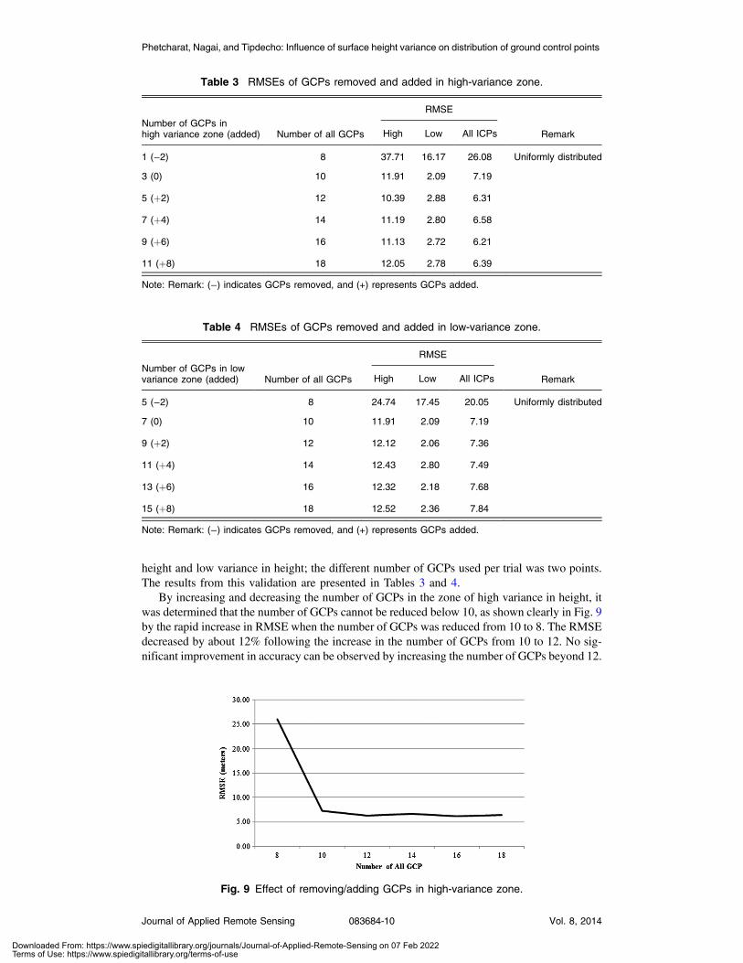
height and low variance in height; the different number of GCPs used per trial was two points.The results from this validation are presented in Tables 3 and 4.

By increasing and decreasing the number of GCPs in the zone of high variance in height, itwas determined that the number of GCPs cannot be reduced below 10, as shown clearly in Fig. 9by the rapid increase in RMSE when the number of GCPs was reduced from 10 to 8. The RMSEdecreased by about 12% following the increase in the number of GCPs from 10 to 12. No sig-nificant improvement in accuracy can be observed by increasing the number of GCPs beyond 12.

Table 3 RMSEs of GCPs removed and added in high-variance zone.

Number of GCPs inhigh variance zone (added) Number of all GCPs

RMSE

RemarkHigh Low All ICPs

1 (−2) 8 37.71 16.17 26.08 Uniformly distributed

3 (0) 10 11.91 2.09 7.19

5 (þ2) 12 10.39 2.88 6.31

7 (þ4) 14 11.19 2.80 6.58

9 (þ6) 16 11.13 2.72 6.21

11 (þ8) 18 12.05 2.78 6.39

Note: Remark: (−) indicates GCPs removed, and (+) represents GCPs added.

Table 4 RMSEs of GCPs removed and added in low-variance zone.

Number of GCPs in lowvariance zone (added) Number of all GCPs

RMSE

RemarkHigh Low All ICPs

5 (−2) 8 24.74 17.45 20.05 Uniformly distributed

7 (0) 10 11.91 2.09 7.19

9 (þ2) 12 12.12 2.06 7.36

11 (þ4) 14 12.43 2.80 7.49

13 (þ6) 16 12.32 2.18 7.68

15 (þ8) 18 12.52 2.36 7.84

Note: Remark: (−) indicates GCPs removed, and (+) represents GCPs added.

Fig. 9 Effect of removing/adding GCPs in high-variance zone.




Increasing or decreasing the number of GCPs in the low variance in height zone resulted inthe same trend found in the high variance in height zone; however, the results did not show anysignificant improvement in accuracy following an increase in the number of GCPs beyond10 (Fig. 10).

7 Conclusions

In this study, an image of mountainous terrain of the Chiang-Mai area acquired by Worldview I,a global DEM, and 78 ground truth points with an accuracy of 0.2 m were used to evaluatethe accuracy of distortion correction using a polynomial model. Using the turning pointfrom the elevation and SD histogram, the terrain was divided into two regions: low variancein height and high variance in height. This study determined the RMSE of the GCPs’ coordinatesand demonstrated that the distribution of the GCPs affects the accuracy. In particular, it wasshown that a uniform distribution of GCPs was the best arrangement. The effect of increasingor decreasing the number of GCPs in the high/low variance in height zones was investigated forthe case of uniform distribution. The results conclude that a suitable minimum number of GCPswas 10 and that the accuracy was improvable by including just two additional GCPs in the zoneof high variance in height, but that increase in the number of GCPs in the zone of low variance inheight offered no significant improvement in accuracy.

The results of this study could be applied to aerial photographs or satellite images as guidancefor identifying the optimum numbers and locations of GCPs for each zone of variance in height,especially for study areas with a variety of surface types. Through this approach, researcherscould save time on the trial-and-error selection of locations for GCPs.

References

1. F. Ayoub et al., “Influence of camera distortions on satellite image registration and changedetection applications,” in IEEE International Geoscience and Remote Sensing Symposium,Vol. 2, pp. 1072–1075 (2008).

2. F. Arif, M. Akbar, and A. M. Wu, “Geometric correction of high resolution satellite imageryand its residual analysis,” in International Conference on Advances in Space Technologies,pp. 162–166 (2006).

3. F. H. Moffitt and E.M. Mikhail, Photogrammetry, 3rd ed., p. 648, Harper & Row, New York(1980).

4. C. Croarkin and P. Tobias, “NIST/SEMATECH e-handbook of statistical methods,” NIST/SEMATECH, 2006, http://www.itl.nist.gov/div898/handbook (24 October 2013).

5. C. Rizos and C. Satirapod, “Differential GPS-how good is it now?,” Meas. Map 15, 28–30(2001).

6. J. Zhang and B. Cheng, “Distribution optimization of ground control points in remote sens-ing image geometric rectification based on cluster analysis,” Proc. SPIE 7497, 749707(2009), http://dx.doi.org/10.1117/12.833671.

Fig. 10 Effect of removing/adding GCPs in low-variance zone.




http://www.itl.nist.gov/div898/handbook




http://dx.doi.org/10.1117/12.833671

http://dx.doi.org/10.1117/12.833671

http://dx.doi.org/10.1117/12.833671

http://dx.doi.org/10.1117/12.833671

http://dx.doi.org/10.1117/12.833671

7. J. Huang and J. Wang, “The selection of GCPs of remote sensing image correction [C],” inEnvironmental Remote Sensing Symposium Academic, pp. 738–742 (2004), http://www.isprs.org/proceedings/XXXV/congress/comm4/papers/446.pdf (24 October 2013).

8. J. Wang et al., “Effect of the sampling design of ground control points on the geometriccorrection of remotely sensed imagery,” Int. J. Appl. Earth Obs. Geoinf. 18(1), 91–100(2012), http://dx.doi.org/10.1016/j.jag.2012.01.001.

9. http://www.digitalglobe.com/resources/satellite-information (October 10 2013).10. A. A. Ahmadi and P. A. Pablo, “Stability of polynomial differential equations: complexity

and converse Lyapunov questions,” IEEE Trans. Autom. Control (Submitted) (2012).11. T. Bayer, R. Winter, and G. Schreier, “Terrain influences in SAR backscatter and attempts to

their correction,” IEEE Trans. Geosci. Remote Sens. 29(3), 451–462 (1991), http://dx.doi.org/10.1109/36.79436.

12. S. Boukharouba, J. M. Rebordao, and P. L. Wendel, “An amplitude segmentation methodbased on the distribution function of an image,” Comput. Vision Graph. Image Process.29(1), 47–59 (1985), http://dx.doi.org/10.1016/S0734-189X(85)90150-1.

13. M. I. Sezan, “A peak detection algorithm and its application to histogram-based image datareduction,” Comput. Vision Graph. Image Process. 49(1), 36–51 (1990), http://dx.doi.org/10.1016/0734-189X(90)90161-N.

14. D. M. Tsai, “A fast thresholding selection procedure for multimodal and unimodal histo-grams,” Pattern Recogn. Lett. 16(6), 653–666 (1995), http://dx.doi.org/10.1016/0167-8655(95)80011-H.

15. Q. Z. Wu, H. Y. Cheng, and B. S. Jeng, “Motion detection via change-point detection forcumulative histograms of ratio images,” Pattern Recogn. Lett. 26(5), 555–563 (2005),http://dx.doi.org/10.1016/j.patrec.2004.09.010.

16. J. H. Han, S. Yang, and B. U. Lee, “A novel 3-D color histogram equalization method withuniform 1-D gray scale histogram,” IEEE Trans. Image Process. 20(2), 506–512 (2011),http://dx.doi.org/10.1109/TIP.2010.2068555.

17. Z. Wangfei et al., “The selection of ground control points in a remote sensing image cor-rection based on weighted Voronoi diagram,” in IEEE Int. Conf. Information Technologyand Computer Science, Vol. 2, pp. 326–329 (2009).

18. K. T. Chang, Introduction to Geographic Information Systems, 3rd ed., McGraw-Hill, NewYork (2006).

Sudniran Phetcharat is a PhD student of the Asian Institute of Technology, Thailand. Hereceived the B.Eng. degree in transportation engineering from Suranaree University ofTechnology, Nakonrachasima, in 1997, and an M.Eng. degree in civil engineering fromKasetsart University, Bangkok, in 2001. He has been an assistant professor with the CivilEngineering Department, Srinakharinwirot University, College Station. His research interestsinclude crumb rubber-modified asphalt, highway materials, GIS application in transportation,and house saving energy.

Masahiko Nagai is an associate director of the Geoinformatics Center and a visiting faculty inthe Asian Institute of Technology (AIT) in Thailand. He received the Master of Science fromAIT and the Doctoral of Engineering from the University of Tokyo, Japan. His research focuseson geoinformatics, mainly environmental monitoring, Earth observation data interoperabilityarrangement with ontological information for remote sensing and GIS, construction of 3-Dmodeling by integrating multiple sensors, as well as disaster management.

Taravudh Tipdecho is a research specialist I (adjunct faculty) at the Asian Institute ofTechnology (AIT) in Thailand. He received his BS and MS degrees from ChiangmaiUniversity, Thailand, and D Tech Sc. degree from AIT, Thailand. His research focuses onthe acquisition methods for large scale geoinformation. In recent years, the research focushas been on information extraction from airborne laser-scanning data. These interests alsoinclude accuracy analysis, image understanding, and object modelling.




http://www.isprs.org/proceedings/XXXV/congress/comm4/papers/446.pdf




http://dx.doi.org/10.1016/j.jag.2012.01.001








http://www.digitalglobe.com/resources/satellite-information



http://dx.doi.org/10.1109/36.79436

http://dx.doi.org/10.1109/36.79436

http://dx.doi.org/10.1109/36.79436

http://dx.doi.org/10.1109/36.79436

http://dx.doi.org/10.1109/36.79436

http://dx.doi.org/10.1016/S0734-189X(85)90150-1

http://dx.doi.org/10.1016/S0734-189X(85)90150-1

http://dx.doi.org/10.1016/S0734-189X(85)90150-1

http://dx.doi.org/10.1016/S0734-189X(85)90150-1

http://dx.doi.org/10.1016/0734-189X(90)90161-N

http://dx.doi.org/10.1016/0734-189X(90)90161-N

http://dx.doi.org/10.1016/0734-189X(90)90161-N

http://dx.doi.org/10.1016/0734-189X(90)90161-N

http://dx.doi.org/10.1016/0734-189X(90)90161-N

http://dx.doi.org/10.1016/0167-8655(95)80011-H

http://dx.doi.org/10.1016/0167-8655(95)80011-H

http://dx.doi.org/10.1016/0167-8655(95)80011-H

http://dx.doi.org/10.1016/0167-8655(95)80011-H

http://dx.doi.org/10.1016/0167-8655(95)80011-H

http://dx.doi.org/10.1016/j.patrec.2004.09.010








http://dx.doi.org/10.1109/TIP.2010.2068555






influence of surface height variance on distribution of ground control

Documents