Influence of Fish Passage Retrofits on Culvert Hydraulic Capacity

Primary Author: Margaret Lang, Ph.D., P.E. Environmental Resources Engineering Humboldt State University

Contributing Author: Eileen Cashman, Ph.D. Environmental Resources Engineering Humboldt State University

Final Report for California Dept. of Transportation (CalTrans)

Contract No.: 43A0068.10

Disclaimer

The contents of this report reflect the views of the authors who are responsible for the facts and accuracy of the data presented herein. The contents do not necessarily reflect the official views or policies of the State of California or the Federal Highway Administration. This report does not constitute a standard, specification, or regulation.

i

ABSTRACT Barriers to migration affect the ease and extent to which fish and other aquatic organisms access required habitat conditions and may affect an organism’s survival and ultimately, a population’s viability. Road-stream crossings, such as culverts bridges and fords, can create passage barriers due to their inherent design or as a result of geomorphic response of streams to their installation. Addressing fish passage at road-stream crossings requires inventorying, assessing and prioritizing retrofit or replacement of existing culvert barriers, and proper design and installation of new culverts and culvert retrofits. Laboratory and field analysis of the effects of fish passage retrofits, such as baffles and weirs, on culvert hydraulic performance has focused primarily on whether the retrofit meets the hydraulic conditions needed for fish passage over the range of flows at which fish are present and attempting to migrate. Retrofitting a culvert barrel to improve fish passage may also alter the hydraulic performance of the culvert at all flows. Few studies have been conducted to specifically measure and quantify the impact of retrofits on culvert hydraulic capacity at flood flows. In these studies, laboratory and field measurements were collected to quantify high flow hydraulic performance of retrofit culverts, develop model parameters and identify appropriate design and analysis methods. Sample applications, updated design parameters and recommended analysis assumptions are described for common design tools (HY8, HEC-RAS, and FishXing V3). Laboratory physical model experiments were also conducted to evaluate sediment transport and trapping characteristics of these retrofit designs over a range of flows. Generally, experimental results indicate trapped sediment in culverts retrofit to improve fish passage decreases the effectiveness of the retrofit due to sediment deposition in areas with lower velocities (where fish can rest). Other observations include:

1. Trapped sediment reduced the effective culvert barrel roughness and, thus, decreased water depths and increased velocities through the culvert, compared to clear water experiments with the retrofit baffles.

2. High flows (culvert barrel water depth/culvert height > 0.5) successfully cleared trapped sediment under conditions of minimal sediment transport from upstream

3. Preliminary results indicate moderate flows (culvert barrel water depth/culvert height ~ 0.25 to 0.5) in combination with moderate sediment feed rates caused the greatest accumulation of trapped sediment

These experiments highlight the importance of including sediment accumulation in design and analysis, and potentially impact design recommendations for culverts retrofit for fish passage and other similar fish passage improvement structures.

ii

ACKNOWLEDGMENTS This work would not have been possible without the hard work and dedication of Humboldt State University’s College of Natural Resources and Sciences technicians and students. Marty Reed (technician) constructed the flume culvert models and kept the flume and pumps functional. Humboldt State University Environmental Resources Engineering students worked on the field and laboratory crews collecting data and performing data analysis: Vernon Bevan, Cameron Bracken, Bryce Cruey, Omar Diaz, Amelia Dillon, Peter Ghiulamila, Katie Gurin, Graham Lierley, Travis May, Jeremy Miller-Schulze, William Semel, Adam Siade, Charles Sharpsteen, Lucas Siegfried, Joey Smith, Jamie Taylor, Daryl Van Dyke, and Ryan Vincente. The Caltrans project manager, Bruce Swanger, provided valuable assistance with project coordination.

iii

TABLE OF CONTENTS

1 INTRODUCTION ................................................................................................................ 1

2 LITERATURE REVIEW .................................................................................................... 4

2.1 PHYSICAL MODEL EXPERIMENTS .................................................................................. 4 2.1.1 Circular Culvert Retrofits.......................................................................................... 5 2.1.2 Box Culvert Retrofits ................................................................................................. 8 2.1.3 Other Relevant Physical Model Experiments .......................................................... 11 2.1.4 Experiments incorporating Sediment....................................................................... 13

2.2 SUMMARY OF METHODS IN DESIGN MANUALS AND GUIDANCE DOCUMENTS ........... 14 2.3 SUMMARY OF PROFESSIONAL PRACTICE ..................................................................... 14

3 METHODS.......................................................................................................................... 17

3.1 PHYSICAL MODEL EXPERIMENTS ................................................................................ 17 3.2 SEDIMENT TRANSPORT EXPERIMENTS......................................................................... 25 3.3 FIELD SITE SELECTION AND MONITORING .................................................................. 29 3.4 LABORATORY AND FIELD DATA ANALYSES................................................................ 32

4 RESULTS ............................................................................................................................ 36

4.1 PHYSICAL MODEL EXPERIMENTS – WITHOUT SEDIMENT............................................ 36 4.1.1 Retrofit Impact on Headwater Depth....................................................................... 36 4.1.2 Laboratory-Scale Retrofit Culvert Effective Roughness.......................................... 45 4.1.3 Extension of Empirical Models................................................................................ 53 4.1.4 Vortex Weir Model Results ...................................................................................... 60

4.2 PHYSICAL MODEL EXPERIMENTS – WITH SEDIMENT................................................... 62 4.2.1 Sediment Clearing and Trapping Characteristics ................................................... 62 4.2.2 Fish passage conditions through retrofit culverts with trapped sediment............... 68

4.3 FIELD OBSERVATIONS.................................................................................................. 73 4.3.1 Chadd Creek ............................................................................................................ 74 4.3.2 Clarks Creek ............................................................................................................ 78 4.3.3 Griffin Creek............................................................................................................ 79 4.3.4 John Hatt Creek....................................................................................................... 81 4.3.5 Luffenholtz Creek..................................................................................................... 82 4.3.6 Palmer Creek ........................................................................................................... 84 4.3.7 Peacock Creek ......................................................................................................... 86

5 DISCUSSION AND APPLICATIONS ............................................................................. 88

5.1 APPLICATION OF LABORATORY RESULTS TO FIELD SCALE......................................... 88 5.1.1 Headwater Elevation Impacts.................................................................................. 88 5.1.2 Effective Roughness ................................................................................................. 92 5.1.3 Empirical Design Equations.................................................................................... 95 5.1.4 Analysis of Culverts Longer than the Laboratory Models....................................... 96

5.2 COMPARISON OF BOX CULVERT RETROFIT PERFORMANCE ........................................ 99 5.3 MODELING APPROACHES FOR DESIGN AND ANALYSIS ............................................. 103 5.4 SEDIMENT EFFECTS.................................................................................................... 106

6 SUMMARY....................................................................................................................... 108

7 REFERENCES ................................................................................................................. 110

APPENDICES ARE AVAILABLE AS SEPARATE DOCUMENTS.

iv

LIST OF FIGURES Figure 2-1. Offset baffle design used in the experiments of Rajaratnam et al. (1988). [Figure from Rajaratnam et al. (1988)] ........................................................................................................ 6 Figure 2-2. Depressed invert or embedded culvert showing perimeter regions with different roughness coefficients. .................................................................................................................. 11 Figure 3-1. Baffle geometry variable definitions for the full-spanning angled baffle culvert models. .......................................................................................................................................... 19 Figure 3-2. Baffle geometry variable definitions for the circular culvert with corner baffle retrofit models. .......................................................................................................................................... 19 Figure 3-3. Measuring the water surface profile along the culvert centerline through the circular culvert retrofit................................................................................................................................ 23 Figure 3-4. Looking upstream at the experimental set-up in the flume for a box culvert. ............ 26 Figure 3-5. Sediment size distribution for bed sediment collected from Luffenholtz Creek, Humboldt County, California. ....................................................................................................... 28 Figure 3-6. Sediment size distribution for the sediment mix used in the flume sediment transport experiments. .................................................................................................................................. 28 Figure 3-7. (a) Cork line marking the high water level after a storm flow. (b) Peak stage recorders installed at each site also doubled as staff plates. .......................................................... 31 Figure 3-8. Clay line sets at Chadd Creek. ................................................................................... 31 Figure 3-9. Peacock Ck (Tan Oak Dr, Del Norte Co, CA)............................................................ 34 Figure 3-10. Mixed regions of plunging and streaming flow over a fishway weir. ...................... 35 Figure 3-11. Defining an equivalent V-notch weir for vortex weir geometry............................... 35 Figure 4-1. Retrofit and non-retrofit water surface profiles for the high, close-spaced, full-spanning, angled baffles at the highest experimental flow rate, 0.34 cfs. ..................................... 37 Figure 4-2. Change in relative headwater depth (HWbaffled/HWunbaffled) as a function of flow rate in a model box culvert retrofit with the various height, far-spaced, full-spanning angled baffles. ... 38 Figure 4-3. Change in relative headwater depth (HWbaffled/HWunbaffled) as a function of flow rate in a model box culvert retrofit with the various height, intermediate-spaced, full-spanning angled baffles. ........................................................................................................................................... 39 Figure 4-4. Change in relative headwater depth(HWbaffled/HWunbaffled) as a function of flow rate in a model box culvert retrofit with the various height, close-spaced, full-spanning angled baffles. 40

v

Figure 4-5. Change in relative headwater depth (HWbaffled/HWunbaffled) as a function of flow rate in model box culverts retrofit with partial spanning, constant height baffles with wall angles of 30-, 45- and 60-degrees. ....................................................................................................................... 42 Figure 4-6. Relative change in headwater depth with installation of corner baffles in 6- and 8-inch diameter circular culvert models. .......................................................................................... 43 Figure 4-7. Relative change in headwater depth with installation of vortex weirs in a 1-ft wide x 0.93-ft high arch culvert model. .................................................................................................... 43 Figure 4-8. Relative increase in HW with distance from the inlet to the first baffle for the three baffle heights in the full-spanning, angled baffle culvert models. ................................................ 44 Figure 4-9. Laboratory-scale effective roughness (as Manning’s n) versus relative submergence (water depth / maximum baffle height) for various height, far-spaced, full-spanning angled baffles. ........................................................................................................................................... 46 Figure 4-10. Laboratory-scale effective roughness (as Manning’s n) versus relative submergence (water depth / maximum baffle height) for various height, intermediate-spaced, full-spanning angled baffles. ............................................................................................................................... 47 Figure 4-11. Laboratory-scale effective roughness (as Manning’s n) versus relative submergence (water depth / maximum baffle height) for various height, far-spaced, full-spanning angled baffles. ........................................................................................................................................... 48 Figure 4-12. Laboratory-scale effective roughness (as Manning’s n) versus flow rate for all configurations of the full-spanning angled baffles. ....................................................................... 49 Figure 4-13 Laboratory-scale effective roughness (as Manning’s n) versus relative submergence (water depth / maximum baffle height) for various wall angle, constant height, partial-spanning baffles. ........................................................................................................................................... 51 Figure 4-14. Laboratory-scale effective roughness (as Manning’s n) versus flow rate for the 30-, 45-, and 60-degree wall angle, partial-spanning baffles................................................................ 52 Figure 4-15. Laboratory-scale effective roughness (as Manning’s n) versus relative submergence (water depth / maximum baffle height) for the circular culvert model retrofit with corner baffles........................................................................................................................................................ 52 Figure 4-16. Full-spanning, angled baffle retrofit model culvert observations fit

to ( zyCWgSQQ oa

o max 5

* == ) ....................................................................................... 54

Figure 4-17. Full-spanning, angled baffle retrofit model culvert observations fit

to ( zyCWgSQQ oa

o max 5

* == ) ....................................................................................... 55

Figure 4-18. Full-spanning, angled baffle retrofit model culvert observations fit

to ( zyCWgSQQ oa

o max 5

* == ) ....................................................................................... 56

vi

Figure 4-19. Variation of empirical design equation parameters, C and a, for various baffle height and spacing full-spanning, angled baffle retrofits in box culverts................................................. 57 Figure 4-20. Fit of partial spanning angled baffle retrofit data to

( zyCWgSQQ oa

o max 5

* == ) .......................................................................................... 58

Figure 4-21. Fit of all corner baffle model data to determine model parameters for Rajaratnam and Katapodis’ dimensionless equation (Equation 3-2). ............................................................... 59 Figure 4-22. Comparison of corner baffle retrofit model results with C = 8.6 and a = 2.53 values recommended by WDFW (2003) for baffles of this height and spacing....................................... 59 Figure 4-23. Chezy coefficient for model vortex weir fishway in a custom arch culvert. ............ 61 Figure 4-24. A photo showing the sediment accumulation in the high, close-spaced, full-spanning angled baffle culvert model at a slope of 0.5% and a flow of 0.34 cfs. ....................................... 63 Figure 4-25. A photo showing the sediment accumulation in the high, close-spaced, full-spanning angled baffle culvert model at a slope of 2.0% and flows of 0.06, 0.095, 0.195 and 0.34 cfs, respectively from top to bottom. ................................................................................................. 63 Figure 4-26. A photo showing the sediment accumulation in the low, far-spaced, full-spanning angled baffle culvert model at a slope of 2.0% and flows of 0.06, 0.095, 0.195 and 0.34 cfs, respectively, from top to bottom. ................................................................................................ 65 Figure 4-27. A photo showing the sediment accumulation in the custom arch retrofit culvert at a slope of 4.0% and flows of 0.06, 0.095, 0.195 and 0.34 cfs, respectively from top to bottom. .. 66 Figure 4-28. Photos comparing sediment accumulation in all culvert models at 2.0% slope and 0.195 cfs flow. ............................................................................................................................... 67 Figure 4-29. Retrofit water surface profiles with and without sediment for box culvert with high, close-spaced, full-spanning angled baffles. The slope is 0.5% and the measurement flow is 0.195 cfs. ............................................................................................................................................... 69 Figure 4-30. Retrofit water surface profiles with and without sediment for the box culvert model with high, close-spaced, full-spanning angled baffles. ................................................................ 70 Figure 4-31. Mannings roughness coefficients compared between unbaffled, baffled clear water runs and baffled runs with sediment. ........................................................................................... 70 Figure 4-32. Retrofit water surface profiles with and without sediment for the box culvert retrofit with high, close-spaced, full-spanning angled baffles................................................................... 71 Figure 4-33. Retrofit water surface profiles with and without sediment for the custom arch culvert with vortex weirs at the highest experimental flow rate, 0.34 cfs. ................................................ 72 Figure 4-34. Water surface profiles (WSPs) collected at Chadd Creek. ....................................... 75 Figure 4-35. Effective roughness approach model fit for Chadd Creek at 90 cfs. ........................ 76

vii

Figure 4-36. Effective roughness approach model fit for Chadd Creek at 200 cfs. ...................... 76 Figure 4-37. Effective roughness approach model fit for Chadd Creek at 253 cfs. ...................... 76 Figure 4-38. HEC-RAS simulations of the Chadd Creek culvert (HUM101, PM40.12) water surface elevations with weir spacing at 21 ft for Q = 90 and 200 cfs. .......................................... 77 Figure 4-39. HEC-RAS simulations of the Chadd Creek culvert (HUM101, PM40.12) water surface elevations with weir spacing at 10.5 ft for Q = 253 cfs. ................................................... 77 Figure 4-40. Clarks Creek water surface profiles measured in the offset baffle retrofit, right culvert bay. .................................................................................................................................... 78 Figure 4-41. Observed and HY-8 predicted water surface profile through the retrofit, right, bay of the Clarks Creek (DN199, PM2.56) culvert at 55 cfs. .................................................................. 79 Figure 4-42. Observed and HY-8 predicted water surface profile through the retrofit, right, bay of the Clarks Creek (DN199, PM2.56) culvert at 104 cfs. ................................................................ 79 Figure 4-43. Water surface profiles measured through the Griffin Creek culvert (DN199, PM31.31) in Water Year 2006. The corner baffles in the downstream 175 feet of culvert are shown in side view. ....................................................................................................................... 80 Figure 4-44. Water surface profiles measured through the Griffin Creek culvert (DN199, PM31.31) in Water Year 2007. ..................................................................................................... 80 Figure 4-45. High water mark elevations from the January 3-5, 2008 peak flows surveyed at John Hatt Ck (MEN128, PM39.95) on January 17, 2008...................................................................... 82 Figure 4-46. Water surface profiles and partial profiles collected at Luffenholtz Creek (HUM101, PM99.03)....................................................................................................................................... 83 Figure 4-47. Analysis of Luffenholtz Ck (HUM101, PM99.03) water surface profile under streaming flow conditions at 221 cfs............................................................................................. 84 Figure 4-48. Water surface profiles measured at Palmer Creek (HUM101, PM62.22). ............... 85 Figure 4-49. HEC-RAS simulation using n=0.060 for the corner baffle retrofit effective roughness at 44 cfs for Palmer Creek (HUM101, PM62.22). ....................................................... 85 Figure 4-50. HEC-RAS simulation using n=0.060 for the corner baffle retrofit effective roughness at 102 cfs for Palmer Creek (HUM101, PM62.22). ..................................................... 86 Figure 4-51. Predicted and observed water surface elevations over the vortex weirs at Peacock Ck for a discharge of 1.25 cfs. ............................................................................................................ 87 Figure 4-52. Predicted and observed water surface elevations over the vortex weirs at Peacock Ck for a discharge of 6.84 cfs. ............................................................................................................ 87

viii

Figure 5-1. Comparison of HW depths observed in the laboratory for an unbaffled model box culvert 0.5-ft wide by 0.5-ft high to the inlet control HW prediction equations of HDS-5 (FHWA, 2004). Data includes all culvert slopes.......................................................................................... 90 Figure 5-2. Comparison of HW depths observed in the laboratory for the model box culvert retrofit with low, far-spaced, full-spanning angled baffles to the inlet and outlet control HW prediction equations of HDS-5 (FHWA, 2004)............................................................................. 91 Figure 5-3. Comparison of HW depths observed in the laboratory for the model box culvert retrofit with high, close-spaced, full-spanning angled baffles to the inlet and outlet control HW prediction equations of HDS-5 (FHWA, 2004)............................................................................. 92 Figure 5-4. Comparison of field measured and laboratory-derived effective roughness coefficients. ................................................................................................................................... 93 Figure 5-5. Effective roughness versus flow rate for a 6-ft by 6-ft box culvert retrofit with medium height, close-spaced full spanning angle baffles. ............................................................ 96 Figure 5-6. Headwater and water surface elevation simulations for various length laboratory-scale box culverts on 0.5 and 2% slopes retrofit with high height, close-spaced full-spanning angled baffles. ........................................................................................................................................... 98 Figure 5-7. Headwater and water surface elevation simulations for various length field-scale box culverts on a 0.5 and 2% slope retrofit with high height, close-spaced full-spanning angled baffles. ........................................................................................................................................... 98 Figure 5-8. Water surface profiles for the model box culverts retrofit with the three partial-spanning angled baffle retrofits (30-, 45- and 60-degree wall angles) and the low, far-spaced full-spanning angled baffle................................................................................................................. 100 Figure 5-9. Water surface profiles for the model box culverts retrofit with the three partial-spanning angled baffle retrofits (30-, 45- and 60-degree wall angles) and the low, far-spaced full-spanning angled baffle................................................................................................................. 100 Figure 5-10. Water surface profiles for the model box culverts retrofit with the three partial-spanning angled baffle retrofits (30-, 45- and 60-degree wall angles) and the low, far-spaced full-spanning angled baffle................................................................................................................. 100 Figure 5-11. Water surface profiles for the model box culverts retrofit with the three partial-spanning angled baffle retrofits (30-, 45- and 60-degree wall angles) and the low, far-spaced full-spanning angled baffle................................................................................................................. 101 Figure 5-12. Water surface profiles for the model box culverts retrofit with the three partial-spanning angled baffle retrofits (30-, 45- and 60-degree wall angles) and the low, far-spaced full-spanning angled baffle................................................................................................................. 102 Figure 5-13. Water surface profiles for the model box culverts retrofit with the three partial-spanning angled baffle retrofits (30-, 45- and 60-degree wall angles) and the low, far-spaced full-spanning angled baffle................................................................................................................. 102

ix

Figure 5-14. Predicted headwater and water surface elevations through the 8-ft x 8-ft culvert for flow rates from 200 to 500 cfs..................................................................................................... 105 Figure 5-15. Observed sediment accumulation in the custom arch culvert with vortex weirs at the 4.0% slope and highest armoring flow of 0.34 cfs. ..................................................................... 106 Figure 5-16. Peacock Creek field site. ....................................................................................... 107

x

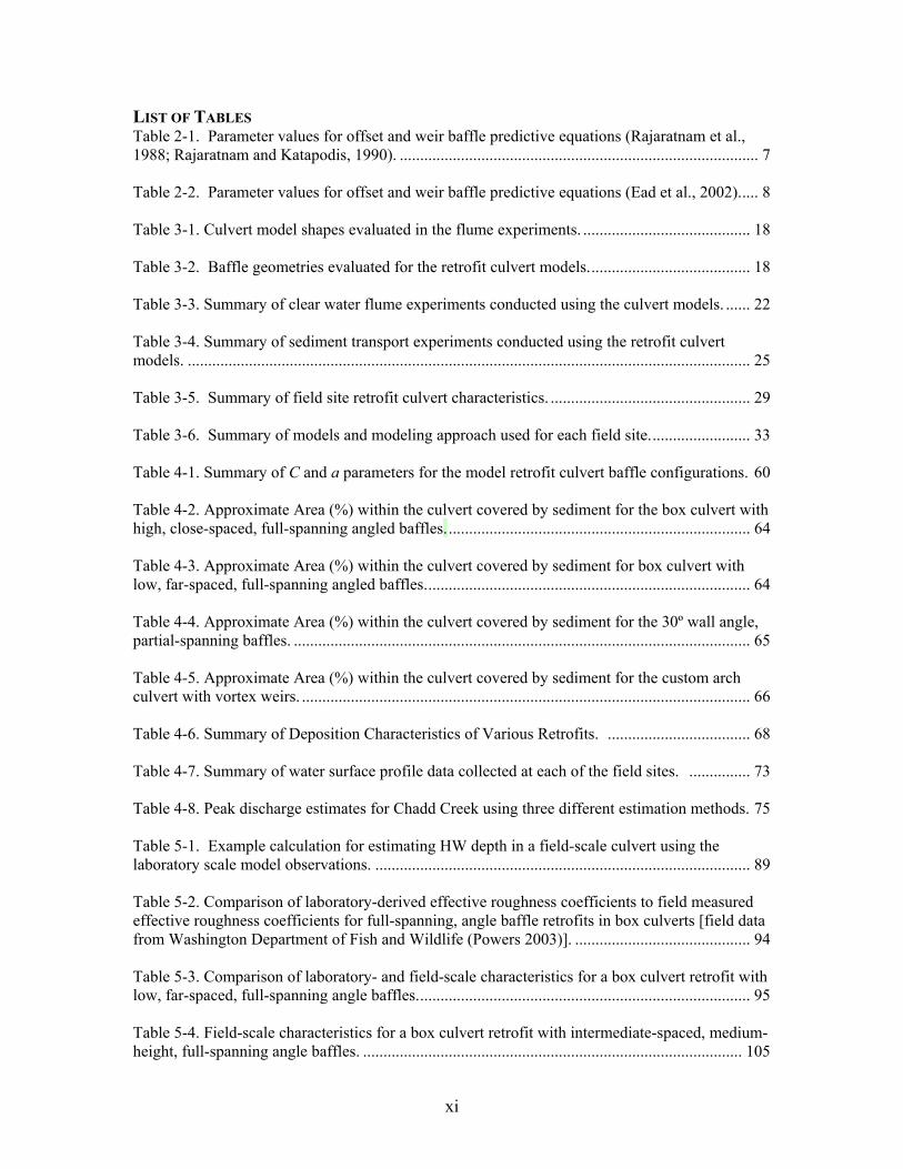
LIST OF TABLES Table 2-1. Parameter values for offset and weir baffle predictive equations (Rajaratnam et al., 1988; Rajaratnam and Katapodis, 1990). ........................................................................................ 7 Table 2-2. Parameter values for offset and weir baffle predictive equations (Ead et al., 2002)..... 8 Table 3-1. Culvert model shapes evaluated in the flume experiments. ......................................... 18 Table 3-2. Baffle geometries evaluated for the retrofit culvert models........................................ 18 Table 3-3. Summary of clear water flume experiments conducted using the culvert models. ...... 22 Table 3-4. Summary of sediment transport experiments conducted using the retrofit culvert models. .......................................................................................................................................... 25 Table 3-5. Summary of field site retrofit culvert characteristics. ................................................. 29 Table 3-6. Summary of models and modeling approach used for each field site......................... 33 Table 4-1. Summary of C and a parameters for the model retrofit culvert baffle configurations. 60 Table 4-2. Approximate Area (%) within the culvert covered by sediment for the box culvert with high, close-spaced, full-spanning angled baffles........................................................................... 64 Table 4-3. Approximate Area (%) within the culvert covered by sediment for box culvert with low, far-spaced, full-spanning angled baffles................................................................................ 64 Table 4-4. Approximate Area (%) within the culvert covered by sediment for the 30º wall angle, partial-spanning baffles. ................................................................................................................ 65 Table 4-5. Approximate Area (%) within the culvert covered by sediment for the custom arch culvert with vortex weirs. .............................................................................................................. 66 Table 4-6. Summary of Deposition Characteristics of Various Retrofits. ................................... 68 Table 4-7. Summary of water surface profile data collected at each of the field sites. ............... 73 Table 4-8. Peak discharge estimates for Chadd Creek using three different estimation methods. 75 Table 5-1. Example calculation for estimating HW depth in a field-scale culvert using the laboratory scale model observations. ............................................................................................ 89 Table 5-2. Comparison of laboratory-derived effective roughness coefficients to field measured effective roughness coefficients for full-spanning, angle baffle retrofits in box culverts [field data from Washington Department of Fish and Wildlife (Powers 2003)]. ........................................... 94 Table 5-3. Comparison of laboratory- and field-scale characteristics for a box culvert retrofit with low, far-spaced, full-spanning angle baffles.................................................................................. 95 Table 5-4. Field-scale characteristics for a box culvert retrofit with intermediate-spaced, medium-height, full-spanning angle baffles. ............................................................................................. 105

xi

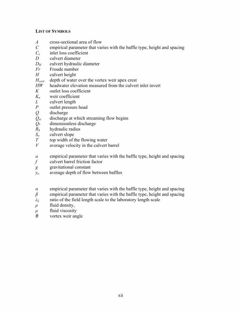
LIST OF SYMBOLS A cross-sectional area of flow C empirical parameter that varies with the baffle type, height and spacing Ce inlet loss coefficient D culvert diameter DH culvert hydraulic diameter Fr Froude number H culvert height Hweir depth of water over the vortex weir apex crest HW headwater elevation measured from the culvert inlet invert K outlet loss coefficient Ku weir coefficient L culvert length P outlet pressure head Q discharge Qst discharge at which streaming flow begins Q* dimensionless discharge Rh hydraulic radius So culvert slope T top width of the flowing water V average velocity in the culvert barrel a empirical parameter that varies with the baffle type, height and spacing f culvert barrel friction factor g gravitational constant yo average depth of flow between baffles α empirical parameter that varies with the baffle type, height and spacing β empirical parameter that varies with the baffle type, height and spacing λL ratio of the field length scale to the laboratory length scale ρ fluid density, μ fluid viscosity θ vortex weir angle

xii

1 Introduction It is well established that resident and anadromous salmonids need access to and from streams as well as unimpaired movement within a stream to access suitable habitat. Barriers to migration affect the ease and extent to which fish and other aquatic organisms access required habitat conditions and may affect an organism’s likelihood for survival and ultimately, a population’s viability. Barriers are defined as any obstacle that prevents or impedes fish from successful passage upstream or downstream (Evans and Johnson 1972), and can be natural or man-made. Some examples of natural barriers are waterfalls, debris jams, or temperature barriers. Artificial, or man-made, barriers to salmonid migration include stream crossings (culverts, bridges, and fords), irrigation diversions and dams. Culverts are a major category of stream crossing structures that can impede or block the movement of fish within a stream. Culverts that are not properly sized, installed, or maintained can cause passage problems such as excessive water velocities through the culvert, downstream channel scour, perched culvert outlets, lack of water depth within a culvert and debris accumulation. These channel and culvert hydraulic conditions or changes in stream channel morphology can cause severe impediments to fish migration and movement within a stream or watershed. Efforts to develop and incorporate fish passage criteria into the design of culverts and other road-stream crossings have been ongoing for many decades. State and federal resource and transportation agencies develop design guidelines specifying methods and hydraulic criteria needed for fish passage. In California, Caltrans (formerly the Division of Highways) implemented a research project in collaboration with the California Department of Fish and Game in 1970 to develop design criteria for passing adult anadromous salmonids through State Highway drainage structures (Kay and Lewis 1970). During this same era, the U.S. Forest Service began a series of systematic culvert inventories and corrections on National Forest lands in California (Evans and Johnson 1972). The basis for fish passage criteria remained similar to recommendations from these early works until recently when the California Department of Fish and Game (2002) and NOAA-Fisheries (NMFS 2001) updated and published new criteria for fish passage in California. Updates to the fish passage criteria were motivated by several factors but the consideration of resident and juvenile salmonid passage needs had the greatest impact on the most recent fish passage criteria and culvert design guidelines. Instream movements of juvenile and non-anadromous salmonids are highly variable and still poorly understood. Juvenile coho salmon spend approximately one year in freshwater before migrating to the ocean and juvenile steelhead may rear in freshwater for up to four years before out-migration; one to two years is common in California. Because much of their life history is spent in freshwater, juveniles of both species are highly dependent on instream habitat. For over-wintering juvenile coho, a common strategy is to migrate out of larger river systems into smaller streams, during late-fall and early-winter storms. Although reasons for this behavior are not certain, juvenile coho may migrate upstream to find more suitable overwintering habitat, away from higher flows and potentially higher turbidity levels found in mainstem channels (Skeesick 1970; Cederholm and Scarlett 1981; Tripp and McCart 1983; Tschaplinski and Hartman 1983;

1

Scarlett and Cederholm 1984; Sandercock 1991; Nickelson et al. 1992). During summer months in western Washington State, juvenile salmonids that moved upstream grew faster than both non-moving and downstream moving juveniles, demonstrating that this behavior may play an important role in the overall heath of the population (Kahler et al. 2001). Similar research in Oregon found a strong correlation between coho smolt size and overwintering location with larger smolts overwintering in small tributaries (Ebersole et al. 2006). Culvert designs that are intended to provide passage for all anadromous life stages have been presented in several detailed design manuals developed by various government agencies that oversee fisheries and road construction and maintenance (e.g., WDFW 2003; British Columbia Ministry of Forests 2002; Baker and Votapka 1990). Thus, properly designed and constructed new culverts should not present migration problems. Existing culverts, however, continue to act as barriers to fish passage because:

• Earlier designs tended to target passage of only adult anadromous salmonids, failing to address the needs of migrating juvenile or non-anadromous salmonids,

• Culverts designed to provide fish passage have frequently been incorrectly installed and improperly maintained,

• Changes in stream morphology often create conditions that hinder fish passage at culverts, and

• Opportunities for improving fish passage are lost due to the “emergency” status of culvert replacements following flood events.

Solving fish passage problems at existing culverts can be accomplished by either full culvert replacement or modification to the existing structure and possibly the adjacent channel. Replacing an existing structure with one designed for fish passage is the most effective solution but modification to the existing structure generally costs significantly less than full replacement. Selecting the appropriate solution is site specific taking into account the current structure’s age and condition, the degree of fish passage that can be restored by modification compared to replacement, the fish species and populations impacted, upstream habitat quality and quantity, and the relative cost of replacement compared to retrofit. The solution adopted for a particular site is generally decided through engineering analysis and consultation with the relevant resource agencies. If modification of the existing structure is selected, this often includes a retrofit to the existing culvert barrel to increase water depth and decrease velocities at fish passage flows. Retrofits generally take the form of baffles or weirs of a specific shape, size and spacing installed along the culvert barrel to achieve water depth and/or velocity criteria for fish passage. Engineers designing culvert retrofits need to be concerned about performance of the retrofits throughout the range of fish passage flows and at flood

2

flows. Alteration of the culvert barrel may impact the high flow performance of an existing culvert and methods to estimate this impact are not well developed or tested. This study was undertaken to develop and evaluate methods for analyzing the hydraulic performance of retrofit culverts. Quantifying the impact of culvert barrel retrofits on a culvert’s flood flow capacity was of particular interest. The study used both laboratory and field measurements to address this question. In the laboratory, physical models of retrofit culverts were installed in a tilting flume to measure hydraulic performance and capacity changes over a wide range of flow and slope conditions. Model box, circular and arch culverts retrofit with a variety of weir and baffle shapes were tested. The laboratory experiments allowed measurements of retrofit culvert hydraulic performance at both fish passage and flood flows. Laboratory experiments were initially conducted with only water in the flume, but the study was extended to include preliminary experiments to compare sediment transport and trapping characteristics of the different retrofit types. Additional measurements were collected at full-scale, retrofit culvert field sites to verify laboratory observations and evaluate the performance of laboratory derived methods or model parameters in predicting field-scale hydraulic performance.

3

2 Literature Review Experimental and field analysis of the effects of fish passage retrofits on culvert hydraulic performance has focused primarily on whether the retrofit meets the hydraulic conditions needed for fish passage over the range of flows at which fish are present and attempting to migrate. Retrofitting a culvert barrel to improve fish passage conditions may also alter the hydraulic performance of the culvert at all flows. Few studies have been conducted to specifically measure and quantify the impact of retrofits on culvert hydraulic capacity at flood flows. Currently, engineers responsible for designing and evaluating culvert retrofits for fish passage use a variety of conservative assumptions to estimate the potential changes in hydraulic capacity. This literature review summarizes all literature found that directly addresses, or potentially contributes to, the analysis of culvert hydraulic capacity changes at flood flows due to culvert barrel retrofits for fish passage. Pertinent research using flume and physical modeling was identified but only limited field measurements were found. In addition to published research, the approaches currently recommended in design manuals or used by practicing professionals are also summarized. This literature review does not cover the extensive literature pertaining to design of baffles, fish ladders and other culvert modifications to improve fish passage through culverts.

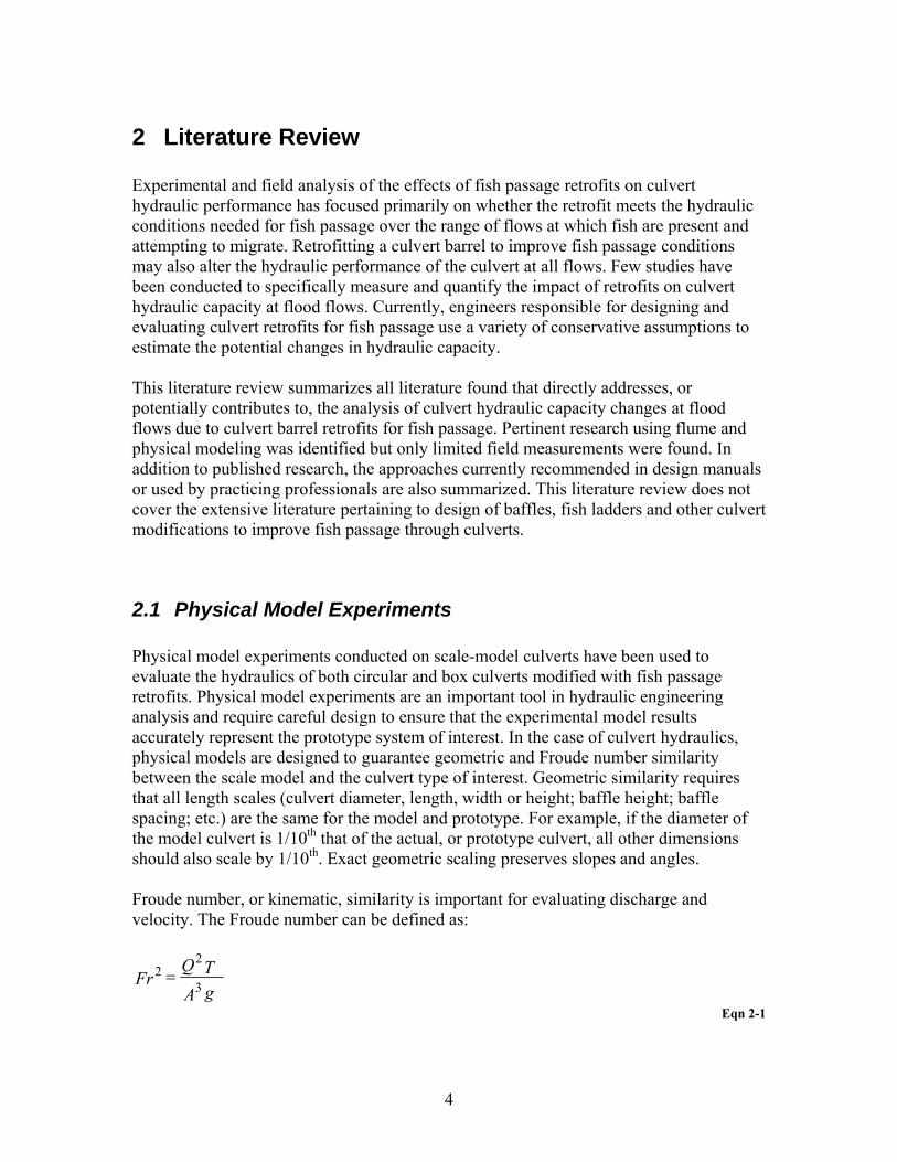
2.1 Physical Model Experiments Physical model experiments conducted on scale-model culverts have been used to evaluate the hydraulics of both circular and box culverts modified with fish passage retrofits. Physical model experiments are an important tool in hydraulic engineering analysis and require careful design to ensure that the experimental model results accurately represent the prototype system of interest. In the case of culvert hydraulics, physical models are designed to guarantee geometric and Froude number similarity between the scale model and the culvert type of interest. Geometric similarity requires that all length scales (culvert diameter, length, width or height; baffle height; baffle spacing; etc.) are the same for the model and prototype. For example, if the diameter of the model culvert is 1/10th that of the actual, or prototype culvert, all other dimensions should also scale by 1/10th. Exact geometric scaling preserves slopes and angles. Froude number, or kinematic, similarity is important for evaluating discharge and velocity. The Froude number can be defined as:

gATQ

Fr 3

22 =

Eqn 2-1

4

where Q is the discharge, T is the top width of the flowing water, A is the cross-sectional area of flow, and g is the gravitational constant. The Froude number is dimensionless so any consistent set of units can be applied. Using the Froude number, the velocity or discharge measured in the model culvert can be used to predict the average velocity or discharge in the prototype culvert at the same relative depth of flow. For strict equivalency between model and prototype systems, one would also have to achieve dynamic similarity or matching Reynolds (Re) number:

μρ DV H

Re =

Eqn 2-2 where ρ is the fluid density, V is the average channel velocity, DH is the hydraulic diameter, and μ is the fluid viscosity. Dynamic similarity is not possible for open channel flow models due to limitations imposed by the fluid properties (density and viscosity). The error introduced by failing to maintain strict Reynolds number similarity is minimized by maintaining Re as high as possible in the model runs and in the same flow regime, laminar or turbulent, as the prototype system. Several physical model experiments conducted at flows approaching flood capacities and which developed relationships appropriate for design level analysis were identified. Rajaratnam, Katapodis and colleagues (Rajaratnam and Katapodis 1990; Rajaratnam et al. 1988, 1989, 1990, 1991) conducted extensive experiments on various baffle configurations in circular culverts with the model culverts flowing up to 80% full. Shoemaker (1956) performed flume experiments with retrofit box culverts to specifically evaluate flood flow hydraulic capacity changes and develop predictive equations for design and analysis. These studies and the resulting design equations are summarized in this section.

2.1.1 Circular Culvert Retrofits Rajaratnam, Katopodis and colleagues (Rajaratnam and Katapodis 1990; Rajaratnam et al. 1988, 1989, 1990, 1991) performed physical model experiments to evaluate the effects of different baffle configurations on the hydraulic conditions in culverts modified for fish passage. Field observations were also made at one retrofit culvert. Their experiments were primarily intended to develop predictive equations for water depth and velocity under fish passage flow conditions but for some baffle configurations their experiments did extend to water depths up to 80% of the culvert diameter. Results from these larger flows have been used to estimate the impacts of baffles on culvert hydraulic capacity for moderate flood flows. The results from these experiments were further refined by Ead et al. (2002) to develop a general correlation between dimensionless discharge and relative depth of flow.

5

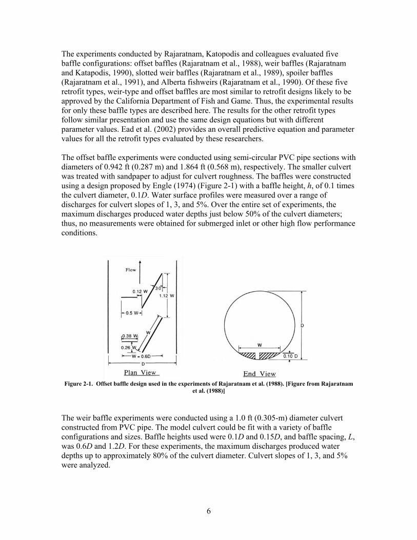
The experiments conducted by Rajaratnam, Katopodis and colleagues evaluated five baffle configurations: offset baffles (Rajaratnam et al., 1988), weir baffles (Rajaratnam and Katapodis, 1990), slotted weir baffles (Rajaratnam et al., 1989), spoiler baffles (Rajaratnam et al., 1991), and Alberta fishweirs (Rajaratnam et al., 1990). Of these five retrofit types, weir-type and offset baffles are most similar to retrofit designs likely to be approved by the California Department of Fish and Game. Thus, the experimental results for only these baffle types are described here. The results for the other retrofit types follow similar presentation and use the same design equations but with different parameter values. Ead et al. (2002) provides an overall predictive equation and parameter values for all the retrofit types evaluated by these researchers. The offset baffle experiments were conducted using semi-circular PVC pipe sections with diameters of 0.942 ft (0.287 m) and 1.864 ft (0.568 m), respectively. The smaller culvert was treated with sandpaper to adjust for culvert roughness. The baffles were constructed using a design proposed by Engle (1974) (Figure 2-1) with a baffle height, h, of 0.1 times the culvert diameter, 0.1D. Water surface profiles were measured over a range of discharges for culvert slopes of 1, 3, and 5%. Over the entire set of experiments, the maximum discharges produced water depths just below 50% of the culvert diameters; thus, no measurements were obtained for submerged inlet or other high flow performance conditions.

Figure 2-1. Offset baffle design used in the experiments of Rajaratnam et al. (1988). [Figure from Rajaratnam

et al. (1988)] The weir baffle experiments were conducted using a 1.0 ft (0.305-m) diameter culvert constructed from PVC pipe. The model culvert could be fit with a variety of baffle configurations and sizes. Baffle heights used were 0.1D and 0.15D, and baffle spacing, L, was 0.6D and 1.2D. For these experiments, the maximum discharges produced water depths up to approximately 80% of the culvert diameter. Culvert slopes of 1, 3, and 5% were analyzed.

6

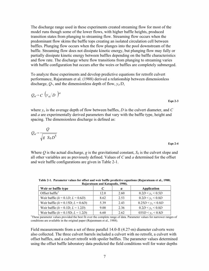
The discharge range used in these experiments created streaming flow for most of the model runs though some of the lower flows, with higher baffle heights, produced transition states from plunging to streaming flow. Streaming flow occurs when the predominant flow skims the baffle tops creating an isolated circulation cell between baffles. Plunging flow occurs when the flow plunges into the pool downstream of the baffle. Streaming flow does not dissipate kinetic energy, but plunging flow may fully or partially dissipate kinetic energy between baffles depending on the baffle characteristics and flow rate. The discharge where flow transitions from plunging to streaming varies with baffle configuration but occurs after the weirs or baffles are completely submerged. To analyze these experiments and develop predictive equations for retrofit culvert performance, Rajaratnam et al. (1988) derived a relationship between dimensionless discharge, Q*, and the dimensionless depth of flow, yo/D,

( DyCQ oa

** = )

Eqn 2-3 where yo is the average depth of flow between baffles, D is the culvert diameter, and C and a are experimentally derived parameters that vary with the baffle type, height and spacing. The dimensionless discharge is defined as:

DSg

QQ

50

** =

Eqn 2-4 Where Q is the actual discharge, g is the gravitational constant, S0 is the culvert slope and all other variables are as previously defined. Values of C and a determined for the offset and weir baffle configurations are given in Table 2-1.

Table 2-1. Parameter values for offset and weir baffle predictive equations (Rajaratnam et al., 1988; Rajaratnam and Katapodis, 1990).

Weir or baffle type C a Application Offset baffle1 12.0 2.60 0.2D < yo < 0.5D Weir baffle (h = 0.1D; L = 0.6D) 8.62 2.53 0.2D < yo < 0.8D Weir baffle (h = 0.15D; L = 0.6D) 5.39 2.43 0.25D < yo < 0.8D Weir baffle (h = 0.1D; L = 1.2D) 9.00 2.36 0.2D < yo < 0.8D Weir baffle (h = 0.15D; L = 1.2D) 6.60 2.62 035D < yo < 0.8D

1These parameter values provided the best fit over the complete range of data. Parameter values for narrower ranges of conditions are available in the original paper (Rajaratnam et al., 1988). Field measurements from a set of three parallel 14.0-ft (4.27-m) diameter culverts were also collected. The three culvert barrels included a culvert with no retrofit, a culvert with offset baffles, and a culvert retrofit with spoiler baffles. The parameter values determined using the offset baffle laboratory data predicted the field conditions well for water depths

7

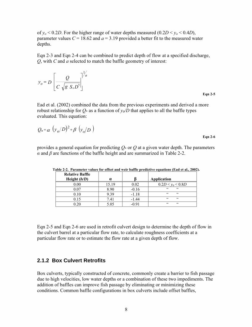
of yo < 0.2D. For the higher range of water depths measured (0.2D < yo < 0.4D), parameter values C = 18.62 and a = 3.19 provided a better fit to the measured water depths. Eqn 2-3 and Eqn 2-4 can be combined to predict depth of flow at a specified discharge, Q, with C and a selected to match the baffle geometry of interest:

⎥⎥

⎦

⎤

⎢⎢

⎣

⎡=

DSgC

QDy

o

a

o 5

1

Eqn 2-5 Ead et al. (2002) combined the data from the previous experiments and derived a more robust relationship for Q* as a function of y0/D that applies to all the baffle types evaluated. This equation:

( ) ( DyDyQ oo βα += 2 * )

Eqn 2-6 provides a general equation for predicting Q* or Q at a given water depth. The parameters α and β are functions of the baffle height and are summarized in Table 2-2.

Table 2-2. Parameter values for offset and weir baffle predictive equations (Ead et al., 2002). Relative Baffle Height (h/D) α β Application

0.00 15.19 0.02 0.2D < y0 < 0.8D 0.07 8.90 -0.16 “ “ 0.10 9.39 -1.18 “ “ 0.15 7.41 -1.44 “ “ 0.20 5.05 -0.91 “ “

Eqn 2-5 and Eqn 2-6 are used in retrofit culvert design to determine the depth of flow in the culvert barrel at a particular flow rate, to calculate roughness coefficients at a particular flow rate or to estimate the flow rate at a given depth of flow.

2.1.2 Box Culvert Retrofits Box culverts, typically constructed of concrete, commonly create a barrier to fish passage due to high velocities, low water depths or a combination of these two impediments. The addition of baffles can improve fish passage by eliminating or minimizing these conditions. Common baffle configurations in box culverts include offset baffles,

8

transverse baffles with notches, and other weir-type baffles. For weir-type baffles, the design principal is to use baffles to create consecutive pools through the culvert barrel (Shoemaker, 1956). Baffle height and spacing are selected to match passage criteria for the fish species of interest by controlling:

• the minimum depth of flow at the upstream end of the pool created between baffles,

• the minimum length of each pool, and • the maximum elevation difference between consecutive pools.

Unlike the experiments conducted by Rajaratnam, Katapodis and colleagues, Shoemaker (1956) conducted experiments to explicitly evaluate changes in culvert hydraulic capacity at flood flows with submerged inlet conditions for concrete box culverts modified with full-spanning, transverse baffles. These experiments were conducted to:

• identify the most hydraulically efficient baffle shapes and heights, • determine the effects of baffle spacing, and • develop design equations to predict the culvert hydraulic capacity after baffle

installation. Shoemaker’s experiments were conducted using plexiglass culvert models with 4-in by 4-in (0.10-m by 0.10-m) square cross-section, and culvert barrel lengths of 4.98 ft (1.52 m), 11.64 ft (3.55 m), and 18.31 ft (5.58 m). All culvert models used identical inlet and outlet configurations with 34-degree wingwalls and an apron to reproduce a standard design used by the State of Oregon Department of Transportation. The outlet apron also had baffles (Shoemaker, 1956). To identify the most hydraulically efficient baffle shape and height, Shoemaker conducted experiments with baffles of 0.1, 0.2 and 0.3 times the culvert height and baffle spacing of 1, 2, and 4 times the culvert height. Observations showed that the "magnitude of the restriction of flow caused by a single baffle appeared to be a function of the contraction of the jet issuing from the area directly above the baffle" (Shoemaker, 1956). Thus, baffles with rounded or angled upstream facing tops minimized flow obstruction and were deemed more hydraulically efficient. The experiments to determine the effects of baffle spacing and to develop design equations were conducted together using baffles with a rounded leading edge and a radius of curvature of 0.1 times the baffle height. Shoemaker (1956) used a standard energy loss approach distinguishing the three principal components of energy loss through the culvert: inlet loss, culvert barrel loss and outlet loss. The culvert barrel losses varied with each baffle configuration, and the inlet and outlet loss remained constant. The experiments were conducted with the culvert slope set at horizontal and the model culvert flowing full throughout with submerged inlet and outlet. Measurements were made for a range of discharges that resulted in headwater depths from 1.5 to 7.5 times the culvert height. This experimental setup creates pressurized flow through the entire

9

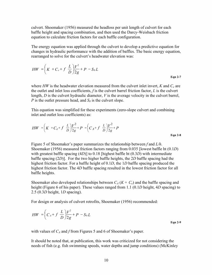
culvert. Shoemaker (1956) measured the headloss per unit length of culvert for each baffle height and spacing combination, and then used the Darcy-Weisbach friction equation to calculate friction factors for each baffle configuration. The energy equation was applied through the culvert to develop a predictive equation for changes in hydraulic performance with the addition of baffles. The basic energy equation, rearranged to solve for the culvert’s headwater elevation was:

LSPgV

DLfCKHW e 0

2

2−+⎟

⎠⎞

⎜⎝⎛ ++=

Eqn 2-7 where HW is the headwater elevation measured from the culvert inlet invert, K and Ce are the outlet and inlet loss coefficients, f is the culvert barrel friction factor, L is the culvert length, D is the culvert hydraulic diameter, V is the average velocity in the culvert barrel, P is the outlet pressure head, and S0 is the culvert slope. This equation was simplified for these experiments (zero-slope culvert and combining inlet and outlet loss coefficients) as:

PVfCPVfCKHW gDL

gDL

Ae +⎟⎠⎞

⎜⎝⎛ +=+⎟

⎠⎞

⎜⎝⎛ ++=

22

22

Eqn 2-8 Figure 5 of Shoemaker’s paper summarizes the relationship between f and L/h. Shoemaker (1956) measured friction factors ranging from 0.035 [lowest baffle ht (0.1D) with greatest baffle spacing (4D)] to 0.18 [highest baffle ht (0.3D) with intermediate baffle spacing (2D)]. For the two higher baffle heights, the 2D baffle spacing had the highest friction factor. For a baffle height of 0.1D, the 1D baffle spacing produced the highest friction factor. The 4D baffle spacing resulted in the lowest friction factor for all baffle heights. Shoemaker also developed relationships between CA (K + Ce) and the baffle spacing and height (Figure 6 of his paper). These values ranged from 1.1 (0.1D height, 4D spacing) to 2.5 (0.3D height, 1D spacing). For design or analysis of culvert retrofits, Shoemaker (1956) recommended:

LSPgV

DLfCHW A 0

2

2−+⎟

⎠⎞

⎜⎝⎛ +=

Eqn 2-9 with values of CA and f from Figures 5 and 6 of Shoemaker’s paper. It should be noted that, at publication, this work was criticized for not considering the needs of fish (e.g. fish swimming speeds, water depths and jump conditions) (McKinley

10

and Webb, 1956). The baffle shapes recommended by Shoemaker, rounded vs. square-topped to promote efficient water flow and the use of transverse baffles spanning the entire box culvert to create consecutive pools were questioned. Thus, the exact baffle shapes and spacing used in the experiments may be inappropriate for fish passage retrofits but the approach for calculating flood flow hydraulic capacity using the friction factors developed in this research appears valid.

2.1.3 Other Relevant Physical Model Experiments

Jordan and Carlson (1987) Design of Depressed Invert Culverts Jordan and Carlson (1987) performed physical model experiments at the Water Research Center of the University of Alaska, Fairbanks to develop a design method for depressed invert culverts. A depressed invert culvert is a culvert with the invert buried below the stream channel bottom (Figure 2-2). The culvert invert is buried with either rip-rap or stream bed material. Their research compared the hydraulic performance of a standard culvert installation to culverts with the invert buried up to 50% of their diameter. The experiments were conducted in a hydraulics flume using 4-inch (0.10-m) and 6-inch (0.15-m) diameter PVC pipe for the model culverts. The culverts were installed flush to a vertical headwall. The culvert backfill material was constructed by gluing a single layer of the appropriate scale of rock (determined by the culvert scale ratio) to the top of a plexiglass insert that occupied the desired embeddedness volume. For all experiments, the embedded material was completely immobile.

Figure 2-2. Depressed invert or embedded culvert showing perimeter regions with different roughness

coefficients. [Figure from FishXing V3 help files (Furniss et al., 2006)] To aid in design of depressed invert culverts, Jordan and Carlson (1987) include the derivation of the culvert cross-section geometric relationships for the non-circular cross-section and the equations needed to determine critical depth. Explicit experiments were

11

conducted to determine:

1. Inlet loss coefficient predictive relationships, 2. Flow resistance of the bed material, and 3. Composite roughness of the culvert barrel.

Experimental measurements were used to determine the inlet and barrel loss coefficients for different percents of embeddedness and compare these loss coefficients to non-embedded culverts. These results could be important for analysis of retrofit culverts if the retrofit or stream geomorphology results in sediment accumulation in the culvert barrel.

McKinley and Webb (1956) Fish Baffle Experiments McKinley and Webb (1956) conducted physical model experiments to identify the baffle configurations that best met fish passage criteria in box culverts. Their research was motivated by a need to improve passage through existing culverts because two commonly used fish passage retrofit types had proven unsuccessful. Placement of low (6- to 8-inch) transverse baffles spanning the bottom of a box culvert (similar to Shoemaker’s experiments described above) to approximate a pool-and-weir fishway had proven ineffective for two reasons. The culvert hydraulics transitioned to streaming flow, creating excessive velocities, at relatively low discharge, and the water depth in the pools between baffles was not sufficient to provide favorable conditions to access the next pool upstream. A second proposed baffle configuration, using alternate partial baffles to create a tortuous flow path through the culvert, also had limited success over the full range of fish passage flows. McKinley and Webb’s (1956) concluded that an offset baffle configuration with 1-ft baffle heights provided the best passage through box culverts and best met their fish passage and culvert performance criteria which included:

• Provide sufficient rest area – large enough to accommodate the numbers of fish with easy access and protection from areas of high velocity

• Achieve complete energy dissipation in each section so that velocity distributions are similar from inlet to outlet

• Provide minimum water depth • Produce a stable flow pattern • Create no objectionable hydraulic features such as whirlpools, hydraulic jumps,

standing waves, etc. • Minimize impacts on hydraulic efficiency • Present no barrier to transport of bed load and debris.

McKinley and Webb (1956) did not develop design equations for predicting the effects of their recommended baffle configuration on hydraulic capacity at flood flows but they did attempt to quantify these effects by comparing hydraulic capacity with and without baffles at high discharges. The high discharges used for these experiments were not defined but qualitatively described as flows that fully submerged the baffles such that

12

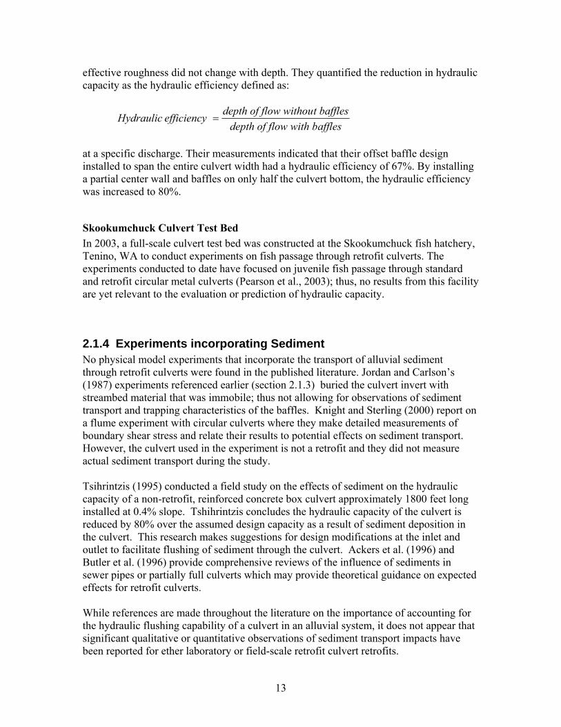
effective roughness did not change with depth. They quantified the reduction in hydraulic capacity as the hydraulic efficiency defined as:

affleslow with bdepth of ft baffleslow withoudepth of fefficiencyHydraulic =

at a specific discharge. Their measurements indicated that their offset baffle design installed to span the entire culvert width had a hydraulic efficiency of 67%. By installing a partial center wall and baffles on only half the culvert bottom, the hydraulic efficiency was increased to 80%.

Skookumchuck Culvert Test Bed In 2003, a full-scale culvert test bed was constructed at the Skookumchuck fish hatchery, Tenino, WA to conduct experiments on fish passage through retrofit culverts. The experiments conducted to date have focused on juvenile fish passage through standard and retrofit circular metal culverts (Pearson et al., 2003); thus, no results from this facility are yet relevant to the evaluation or prediction of hydraulic capacity.

2.1.4 Experiments incorporating Sediment No physical model experiments that incorporate the transport of alluvial sediment through retrofit culverts were found in the published literature. Jordan and Carlson’s (1987) experiments referenced earlier (section 2.1.3) buried the culvert invert with streambed material that was immobile; thus not allowing for observations of sediment transport and trapping characteristics of the baffles. Knight and Sterling (2000) report on a flume experiment with circular culverts where they make detailed measurements of boundary shear stress and relate their results to potential effects on sediment transport. However, the culvert used in the experiment is not a retrofit and they did not measure actual sediment transport during the study. Tsihrintzis (1995) conducted a field study on the effects of sediment on the hydraulic capacity of a non-retrofit, reinforced concrete box culvert approximately 1800 feet long installed at 0.4% slope. Tshihrintzis concludes the hydraulic capacity of the culvert is reduced by 80% over the assumed design capacity as a result of sediment deposition in the culvert. This research makes suggestions for design modifications at the inlet and outlet to facilitate flushing of sediment through the culvert. Ackers et al. (1996) and Butler et al. (1996) provide comprehensive reviews of the influence of sediments in sewer pipes or partially full culverts which may provide theoretical guidance on expected effects for retrofit culverts. While references are made throughout the literature on the importance of accounting for the hydraulic flushing capability of a culvert in an alluvial system, it does not appear that significant qualitative or quantitative observations of sediment transport impacts have been reported for ether laboratory or field-scale retrofit culvert retrofits.

13

2.2 Summary of Methods in Design Manuals and Guidance Documents

Several State Departments’ of Transportation (DOTs) and resource agencies have produced design or guidance manuals (Alaska Dept. of Fish and Game & Alaska Dept. of Transportation 2001; Oregon Dept. of Fish and Wildlife 2004; Caltrans 2007; California Dept. Fish and Game 1998; WDFW 2003) that address culvert retrofits for fish passage improvement. Though fish passage retrofits are described in all of these documents, only two specifically address analysis of hydraulic capacity of culvert retrofits: Washington Department of Fish and Wildlife’s (WDFW) Design of Road Culverts for Fish Passage (WDFW 2003) and Caltrans’ Fish Passage Design for Road Crossings (Caltrans 2007). The WDFW design manual provides the most detailed discussion and recommends using the results from the physical studies of Rajaratnam and Katapodis’ (1990) experiments with weir baffles for circular culverts and Shoemaker’s (1956) findings for box culverts. A summary of both methods, including all relevant equations and equation parameters for recommended retrofit types, are provided in Appendix D of the WDFW design manual (WDFW 2003). The Caltrans design manual does not directly address analysis of hydraulic capacity in retrofit culverts in the chapter on retrofits (Chapter 7) but provides an example in Appendix J. In the example, installation of weirs to retrofit a box culvert are simulated in HEC-RAS as inline structures in a rectangular open channel with the same width as the box culvert. In addition to the State documents, the Federal Highway Administration recently published Design for Fish Passage at Roadway-Stream Crossings: Synthesis Report (Hotchkiss and Frei 2007). However, this document is primarily an overview of the issues that describes the current state of practice and presents guidelines for initiating or improving fish passage programs for State DOTs that have not yet implemented programs.

2.3 Summary of Professional Practice Predicting the effects of culvert baffle installation on high flows is a practical design issue that many hydraulic engineers have encountered. The approaches described in this section summarize methods currently used by hydraulic engineers practicing in the field. This information resulted from a discussion on the Fish Passage mailing list, an online forum for professionals sponsored by the American Fisheries Society Bioengineering Section and hosted by Oregon State University (http://lists.oregonstate.edu/pipermail/fishpass) in July 2005. The discussion was prompted by a query from a forum member following a National Marine Fisheries

14

Service (NMFS) request that baffles be installed on a culvert required to pass a 25-year peak discharge. Initial discussion focused on existing experimental and practical literature on the subject. Contributors referenced the research completed by Rajaratnam, Katopodis and colleagues (Rajaratnam and Katapodis 1990; Rajaratnam et al. 1988, 1989, 1990, 1991), and the methods described in Washington state’s design manual Design of Road Culverts for Fish Passage (WDFW, 2003) discussed above. Two conceptual approaches were described by practitioners:

1. Increasing the effective roughness coefficient for the culvert barrel to account for the increase in barrel frictionloss caused by the presence of baffles, or

2. Reducing the culvert cross-sectional area by the projected area of the installed baffles and calculating a new composite roughness for the culvert.

Both approaches assume that the baffles are fully submerged with streaming, rather than plunging, flow so that the baffles act as roughness elements rather than weirs. This assumption is appropriate for flood flows as streaming flow conditions occur at high flows that completely submerge the baffles. Thus, these analysis methods apply to estimating flood flow culvert performance but may not apply to fish passage flows. Practitioners differed somewhat in their assumptions about baffle roughness and how composite culvert barrel roughness was calculated. The different approaches are summarized below along with the limitations and cautions identified. Two contributors suggested treating the baffles as roughness elements that increased the overall culvert barrel roughness and provided guidelines for determining the new culvert barrel roughness. Patrick Klavas (WDFW) referred to observations from several baffled culverts in Washington State and suggested a general guideline for selecting n-values as a function of flow depth (yo) and baffle height (h). Observed Manning’s roughness values (n) seem to converge to two values. For yo/ h of approximately 1.45, he suggests an n value of 0.084. For yo/ h above 2.8, the suggested value of n is 0.050. A NMFS study (Lang et al. 2004) conducted by Humboldt State University measured roughness coefficients for 3 culverts retrofit with offset baffles and found similar values. For (yo/ h) from 0.6 to 1.95, n was determined to range from 0.039 to 0.107 from a total of 7 observations. The high value, n = 0.107 with yo/ h = 1.3, was an outlier as the next highest n value was 0.076. Contributors agreed that methods used to predict hydraulic capacity should be conservative to ensure reliability. The other recommended analysis method, reducing the culvert cross-sectional area by the projected area of the installed baffles, is similar to the analysis of depressed inlet culverts described above. In this approach, the culvert barrel roughness is calculated as a composite roughness resulting from the sides and bottom of the culvert having different n-values. This method also requires analysis of a culvert with a non-standard cross-section shape. Contributors described the use of hydraulic models and other analytical

15

tools to perform these calculations and recommended roughness values for the false culvert bottom defined by the baffle tops. Many culvert design models allow the user to analyze non-standard culvert cross-section areas by defining the irregular cross-section outline by a set of coordinates. For example, HY8 (FHWA, 2007) allows up to 19 coordinate pairs to describe a non-standard culvert cross-section shape. These coordinate pairs must be determined independent of the culvert hydraulic software and contributors suggested using CAD software or developing spreadsheet macros for common culvert and baffle geometries. Other culvert design models [(e.g. FishXing (Furniss et al., 2006), HEC-RAS (USACE, 2005)] can analyze countersunk or depressed invert culverts, by truncating the culvert cross-section by the depth of embedding. For horizontal baffles, the baffle height can be entered as the embedded depth to simulate the truncated culvert cross-sectional area (similar to Figure 2-2). Once the new culvert cross-section is defined, the additional roughness of the false culvert bottom defined by the baffle tops must be determined. Contributors suggested n-values from 0.035 to 0.045 were reasonable values for the baffle top roughness. The composite roughness resulting from different materials being present on the culvert bottom compared to the sides and top is typically calculated as function of wetted perimeter in contact with each material. The culverts design models internally calculate a composite roughness from either the user provided culvert cross-section geometry (each segment is assigned a roughness coefficient) or from the embedded bottom and culvert material roughness coefficients for the case of embedded culverts. In addition to these suggested approaches, several contributors pointed out that hydraulic capacity of existing culverts was unlikely to be significantly impacted by retrofits because the culvert’s hydraulic capacity would remain inlet controlled. Retrofits are generally used to overcome passage problems associated with steep culverts (>1% slope). If culvert retrofits do not significantly backwater the culvert inlet or otherwise constrict the culvert inlet cross-sectional area, the culvert’s hydraulic capacity should remain unchanged.

16

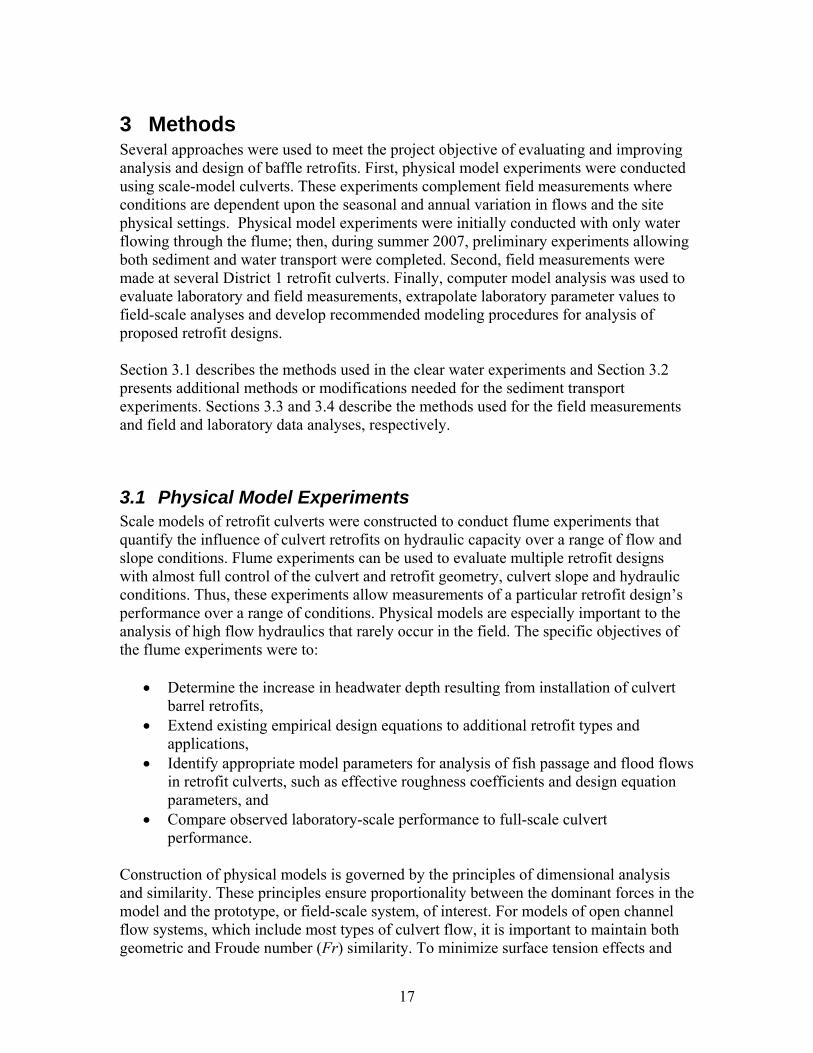
3 Methods Several approaches were used to meet the project objective of evaluating and improving analysis and design of baffle retrofits. First, physical model experiments were conducted using scale-model culverts. These experiments complement field measurements where conditions are dependent upon the seasonal and annual variation in flows and the site physical settings. Physical model experiments were initially conducted with only water flowing through the flume; then, during summer 2007, preliminary experiments allowing both sediment and water transport were completed. Second, field measurements were made at several District 1 retrofit culverts. Finally, computer model analysis was used to evaluate laboratory and field measurements, extrapolate laboratory parameter values to field-scale analyses and develop recommended modeling procedures for analysis of proposed retrofit designs. Section 3.1 describes the methods used in the clear water experiments and Section 3.2 presents additional methods or modifications needed for the sediment transport experiments. Sections 3.3 and 3.4 describe the methods used for the field measurements and field and laboratory data analyses, respectively.

3.1 Physical Model Experiments Scale models of retrofit culverts were constructed to conduct flume experiments that quantify the influence of culvert retrofits on hydraulic capacity over a range of flow and slope conditions. Flume experiments can be used to evaluate multiple retrofit designs with almost full control of the culvert and retrofit geometry, culvert slope and hydraulic conditions. Thus, these experiments allow measurements of a particular retrofit design’s performance over a range of conditions. Physical models are especially important to the analysis of high flow hydraulics that rarely occur in the field. The specific objectives of the flume experiments were to:

• Determine the increase in headwater depth resulting from installation of culvert barrel retrofits,

• Extend existing empirical design equations to additional retrofit types and applications,

• Identify appropriate model parameters for analysis of fish passage and flood flows in retrofit culverts, such as effective roughness coefficients and design equation parameters, and

• Compare observed laboratory-scale performance to full-scale culvert performance.

Construction of physical models is governed by the principles of dimensional analysis and similarity. These principles ensure proportionality between the dominant forces in the model and the prototype, or field-scale system, of interest. For models of open channel flow systems, which include most types of culvert flow, it is important to maintain both geometric and Froude number (Fr) similarity. To minimize surface tension effects and

17

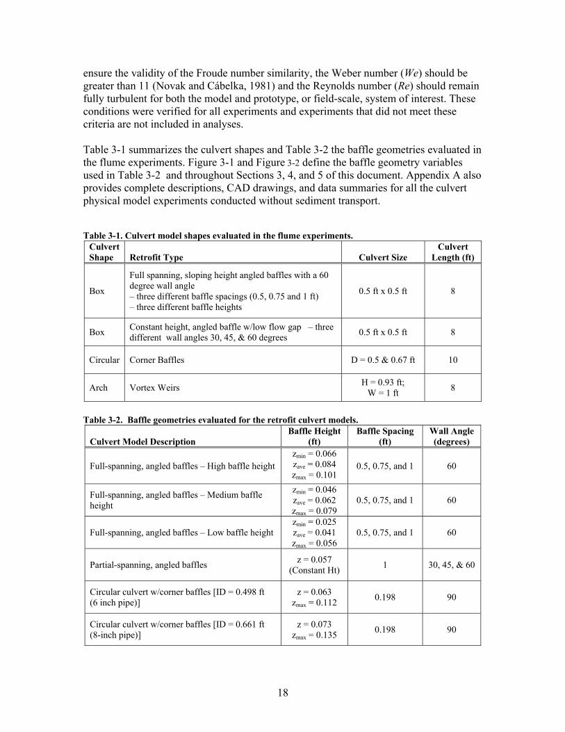
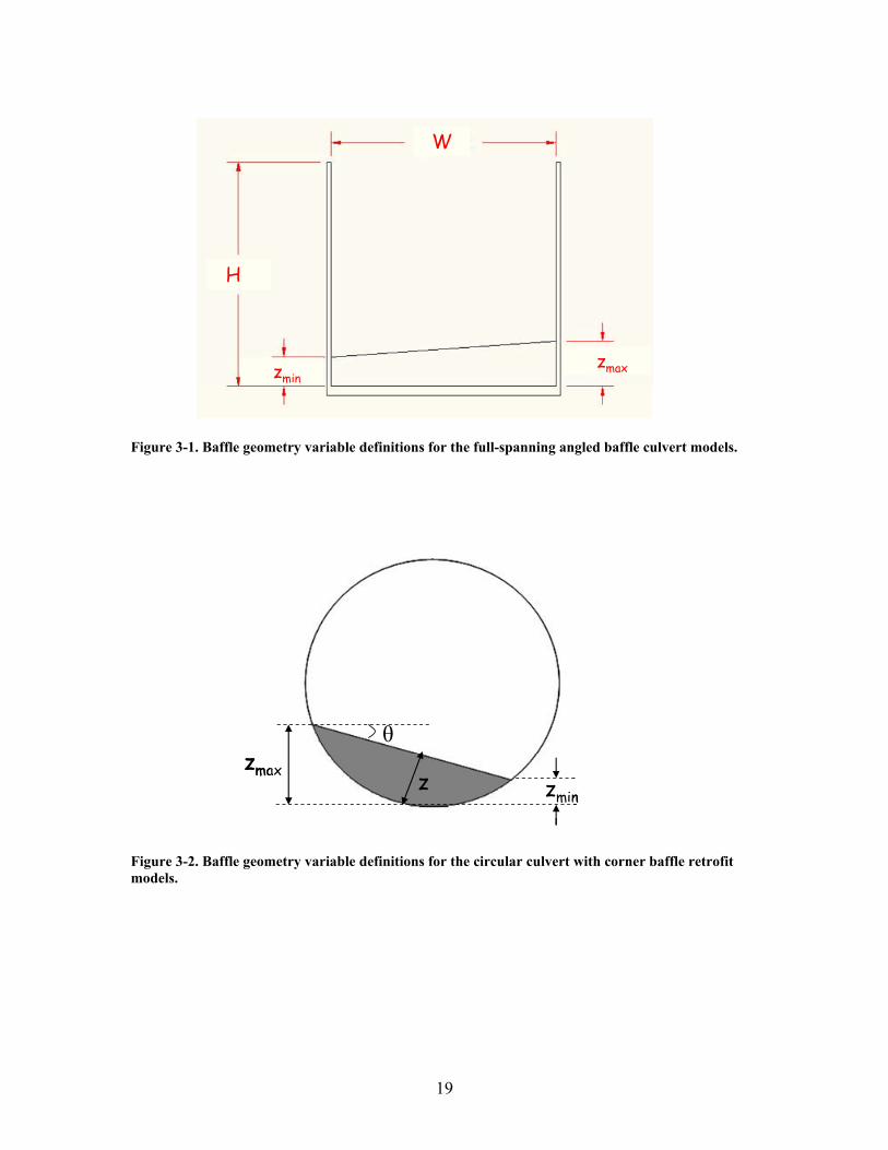
ensure the validity of the Froude number similarity, the Weber number (We) should be greater than 11 (Novak and Cábelka, 1981) and the Reynolds number (Re) should remain fully turbulent for both the model and prototype, or field-scale, system of interest. These conditions were verified for all experiments and experiments that did not meet these criteria are not included in analyses. Table 3-1 summarizes the culvert shapes and Table 3-2 the baffle geometries evaluated in the flume experiments. Figure 3-1 and Figure 3-2 define the baffle geometry variables used in Table 3-2 and throughout Sections 3, 4, and 5 of this document. Appendix A also provides complete descriptions, CAD drawings, and data summaries for all the culvert physical model experiments conducted without sediment transport. Table 3-1. Culvert model shapes evaluated in the flume experiments.

Culvert Shape Retrofit Type Culvert Size

Culvert Length (ft)

Box

Full spanning, sloping height angled baffles with a 60 degree wall angle – three different baffle spacings (0.5, 0.75 and 1 ft) – three different baffle heights

0.5 ft x 0.5 ft 8

Box Constant height, angled baffle w/low flow gap – three different wall angles 30, 45, & 60 degrees 0.5 ft x 0.5 ft 8

Circular Corner Baffles D = 0.5 & 0.67 ft 10

Arch Vortex Weirs H = 0.93 ft; W = 1 ft 8

Table 3-2. Baffle geometries evaluated for the retrofit culvert models.

Culvert Model Description Baffle Height

(ft) Baffle Spacing

(ft) Wall Angle (degrees)

Full-spanning, angled baffles – High baffle height zmin = 0.066 zave = 0.084 zmax = 0.101

0.5, 0.75, and 1 60

Full-spanning, angled baffles – Medium baffle height

zmin = 0.046 zave = 0.062 zmax = 0.079

0.5, 0.75, and 1 60

Full-spanning, angled baffles – Low baffle height zmin = 0.025 zave = 0.041 zmax = 0.056

0.5, 0.75, and 1 60

Partial-spanning, angled baffles z = 0.057 (Constant Ht) 1 30, 45, & 60

Circular culvert w/corner baffles [ID = 0.498 ft (6 inch pipe)]

z = 0.063 zmax = 0.112 0.198 90

Circular culvert w/corner baffles [ID = 0.661 ft (8-inch pipe)]

z = 0.073 zmax = 0.135 0.198 90

18

W

H

zminzmax

W

H

zminzmax

Figure 3-1. Baffle geometry variable definitions for the full-spanning angled baffle culvert models.

zmaxzmin

z

θzmax

zminz

θ

Figure 3-2. Baffle geometry variable definitions for the circular culvert with corner baffle retrofit models.

19

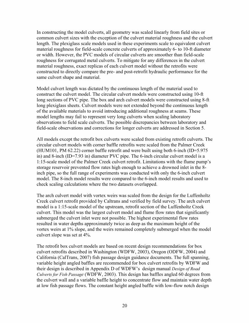
In constructing the model culverts, all geometry was scaled linearly from field sites or common culvert sizes with the exception of the culvert material roughness and the culvert length. The plexiglass scale models used in these experiments scale to equivalent culvert material roughness for field-scale concrete culverts of approximately 6- to 10-ft diameter or width. However, the PVC models of circular culverts are smoother than field-scale roughness for corrugated metal culverts. To mitigate for any differences in the culvert material roughness, exact replicas of each culvert model without the retrofits were constructed to directly compare the pre- and post-retrofit hydraulic performance for the same culvert shape and material. Model culvert length was dictated by the continuous length of the material used to construct the culvert model. The circular culvert models were constructed using 10-ft long sections of PVC pipe. The box and arch culvert models were constructed using 8-ft long plexiglass sheets. Culvert models were not extended beyond the continuous length of the available materials to avoid introducing additional roughness at seams. These model lengths may fail to represent very long culverts when scaling laboratory observations to field scale culverts. The possible discrepancies between laboratory and field-scale observations and corrections for longer culverts are addressed in Section 5. All models except the retrofit box culverts were scaled from existing retrofit culverts. The circular culvert models with corner baffle retrofits were scaled from the Palmer Creek (HUM101, PM 62.22) corner baffle retrofit and were built using both 6-inch (ID=5.975 in) and 8-inch (ID=7.93 in) diameter PVC pipe. The 6-inch circular culvert model is a 1:15-scale model of the Palmer Creek culvert retrofit. Limitations with the flume pump’s storage reservoir prevented flow rates high enough to achieve a drowned inlet in the 8-inch pipe, so the full range of experiments was conducted with only the 6-inch culvert model. The 8-inch model results were compared to the 6-inch model results and used to check scaling calculations where the two datasets overlapped. The arch culvert model with vortex weirs was scaled from the design for the Luffenholtz Creek culvert retrofit provided by Caltrans and verified by field survey. The arch culvert model is a 1:15-scale model of the upstream, retrofit section of the Luffenholtz Creek culvert. This model was the largest culvert model and flume flow rates that significantly submerged the culvert inlet were not possible. The highest experimental flow rates resulted in water depths approximately twice as deep as the maximum height of the vortex weirs at 1% slope, and the weirs remained completely submerged when the model culvert slope was set at 4%. The retrofit box culvert models are based on recent design recommendations for box culvert retrofits described in Washington (WDFW, 2003), Oregon (ODFW, 2004) and California (CalTrans, 2007) fish passage design guidance documents. The full spanning, variable height angled baffles are recommended for box culvert retrofits by WDFW and their design is described in Appendix D of WDFW’s design manual Design of Road Culverts for Fish Passage (WDFW, 2003). This design has baffles angled 60 degrees from the culvert wall and a variable baffle height to concentrate flow and maintain water depth at low fish passage flows. The constant height angled baffle with low-flow notch design

20

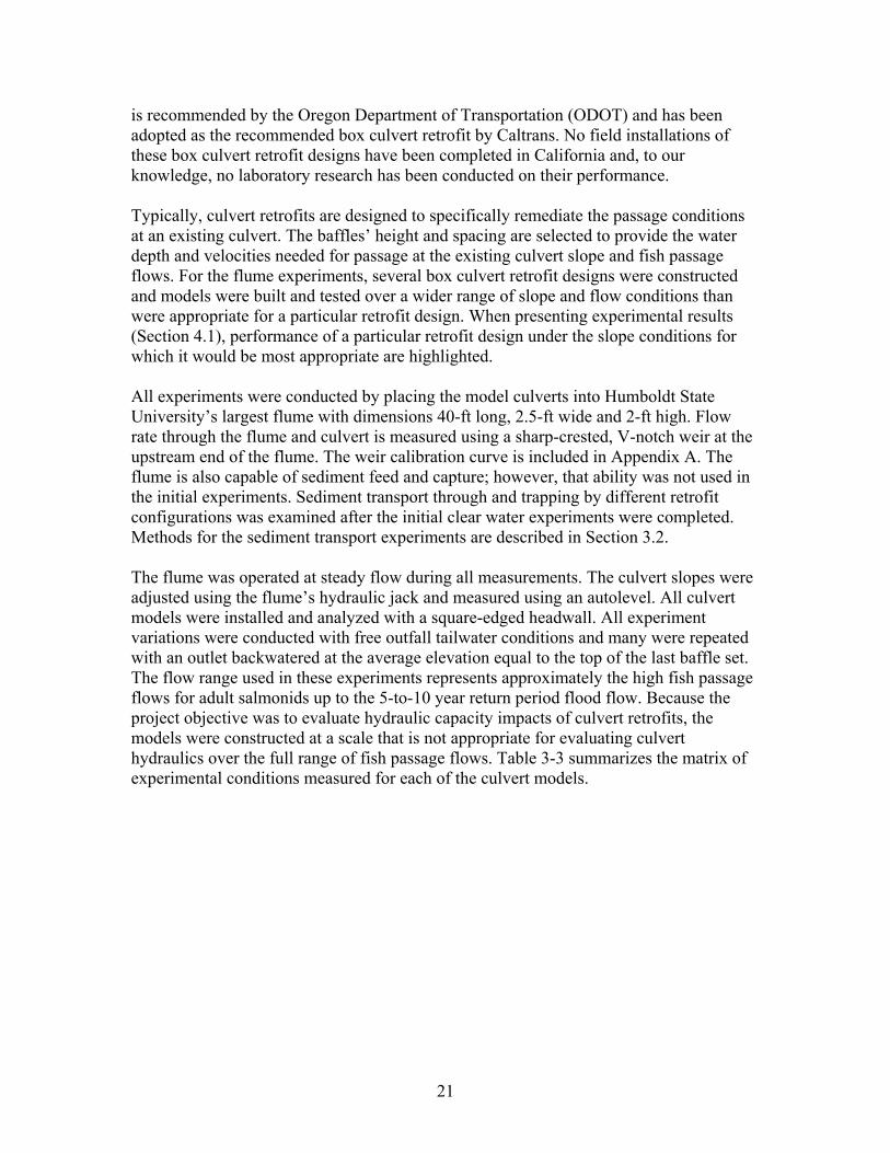
is recommended by the Oregon Department of Transportation (ODOT) and has been adopted as the recommended box culvert retrofit by Caltrans. No field installations of these box culvert retrofit designs have been completed in California and, to our knowledge, no laboratory research has been conducted on their performance. Typically, culvert retrofits are designed to specifically remediate the passage conditions at an existing culvert. The baffles’ height and spacing are selected to provide the water depth and velocities needed for passage at the existing culvert slope and fish passage flows. For the flume experiments, several box culvert retrofit designs were constructed and models were built and tested over a wider range of slope and flow conditions than were appropriate for a particular retrofit design. When presenting experimental results (Section 4.1), performance of a particular retrofit design under the slope conditions for which it would be most appropriate are highlighted. All experiments were conducted by placing the model culverts into Humboldt State University’s largest flume with dimensions 40-ft long, 2.5-ft wide and 2-ft high. Flow rate through the flume and culvert is measured using a sharp-crested, V-notch weir at the upstream end of the flume. The weir calibration curve is included in Appendix A. The flume is also capable of sediment feed and capture; however, that ability was not used in the initial experiments. Sediment transport through and trapping by different retrofit configurations was examined after the initial clear water experiments were completed. Methods for the sediment transport experiments are described in Section 3.2. The flume was operated at steady flow during all measurements. The culvert slopes were adjusted using the flume’s hydraulic jack and measured using an autolevel. All culvert models were installed and analyzed with a square-edged headwall. All experiment variations were conducted with free outfall tailwater conditions and many were repeated with an outlet backwatered at the average elevation equal to the top of the last baffle set. The flow range used in these experiments represents approximately the high fish passage flows for adult salmonids up to the 5-to-10 year return period flood flow. Because the project objective was to evaluate hydraulic capacity impacts of culvert retrofits, the models were constructed at a scale that is not appropriate for evaluating culvert hydraulics over the full range of fish passage flows. Table 3-3 summarizes the matrix of experimental conditions measured for each of the culvert models.

21

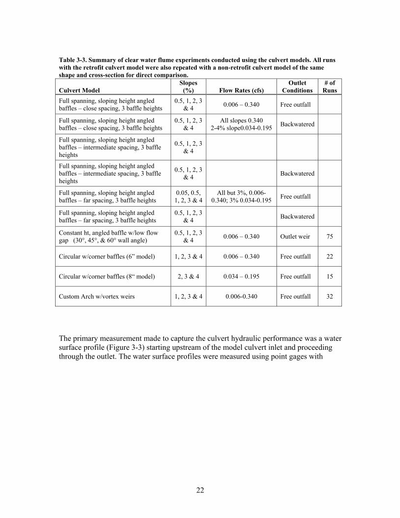
Table 3-3. Summary of clear water flume experiments conducted using the culvert models. All runs with the retrofit culvert model were also repeated with a non-retrofit culvert model of the same shape and cross-section for direct comparison.

Culvert Model Slopes

(%) Flow Rates (cfs) Outlet

Conditions # of

Runs Full spanning, sloping height angled baffles – close spacing, 3 baffle heights

0.5, 1, 2, 3 & 4 0.006 – 0.340 Free outfall

Full spanning, sloping height angled baffles – close spacing, 3 baffle heights

0.5, 1, 2, 3 & 4

All slopes 0.340 2-4% slope0.034-0.195 Backwatered

Full spanning, sloping height angled baffles – intermediate spacing, 3 baffle heights

0.5, 1, 2, 3 & 4

Full spanning, sloping height angled baffles – intermediate spacing, 3 baffle heights

0.5, 1, 2, 3 & 4 Backwatered

Full spanning, sloping height angled baffles – far spacing, 3 baffle heights

0.05, 0.5, 1, 2, 3 & 4

All but 3%, 0.006-0.340; 3% 0.034-0.195 Free outfall

Full spanning, sloping height angled baffles – far spacing, 3 baffle heights

0.5, 1, 2, 3 & 4 Backwatered

Constant ht, angled baffle w/low flow gap (30°, 45°, & 60° wall angle)

0.5, 1, 2, 3 & 4 0.006 – 0.340 Outlet weir 75

Circular w/corner baffles (6” model) 1, 2, 3 & 4 0.006 – 0.340 Free outfall 22

Circular w/corner baffles (8“ model) 2, 3 & 4 0.034 – 0.195 Free outfall 15

Custom Arch w/vortex weirs 1, 2, 3 & 4 0.006-0.340 Free outfall 32

The primary measurement made to capture the culvert hydraulic performance was a water surface profile (Figure 3-3) starting upstream of the model culvert inlet and proceeding through the outlet. The water surface profiles were measured using point gages with

22

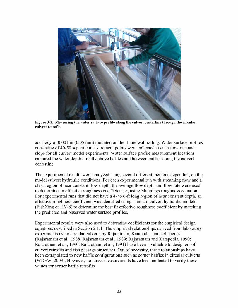
Figure 3-3. Measuring the water surface profile along the culvert centerline through the circular culvert retrofit. accuracy of 0.001 in (0.05 mm) mounted on the flume wall railing. Water surface profiles consisting of 40-50 separate measurement points were collected at each flow rate and slope for all culvert model experiments. Water surface profile measurement locations captured the water depth directly above baffles and between baffles along the culvert centerline. The experimental results were analyzed using several different methods depending on the model culvert hydraulic conditions. For each experimental run with streaming flow and a clear region of near constant flow depth, the average flow depth and flow rate were used to determine an effective roughness coefficient, n, using Mannings roughness equation. For experimental runs that did not have a 4- to 6-ft long region of near constant depth, an effective roughness coefficient was identified using standard culvert hydraulic models (FishXing or HY-8) to determine the best fit effective roughness coefficient by matching the predicted and observed water surface profiles. Experimental results were also used to determine coefficients for the empirical design equations described in Section 2.1.1. The empirical relationships derived from laboratory experiments using circular culverts by Rajaratnam, Katapodis, and colleagues (Rajaratnam et al., 1988; Rajaratnam et al., 1989; Rajaratnam and Katapodis, 1990; Rajaratnam et al., 1990; Rajaratnam et al., 1991) have been invaluable to designers of culvert retrofits and fish passage structures. Out of necessity, these relationships have been extrapolated to new baffle configurations such as corner baffles in circular culverts (WDFW, 2003). However, no direct measurements have been collected to verify these values for corner baffle retrofits.

23

Similar relationships can also be developed for box culvert retrofits but some modification of the non-dimensional relationships is necessary. Rajaratnam et al. (1988) introduced the dimensionless equation:

⎟⎟⎠

⎞⎜⎜⎝

⎛=

D

yCQ o

a

*

Eqn 3-1 where Q* is the dimensionless discharge defined by Rajaratnam et al. (1988) as

DgSQQ o5

* = , yo is the flow depth between baffles, D is the culvert diameter, So is the culvert slope, g is the gravitational constant, and C and a are parameters unique to a given culvert shape and retrofit geometry. This results in a design and analysis equation for circular culverts of the form:

⎟⎟⎠

⎞⎜⎜⎝

⎛==

D

yC

DgS

QQ o

a

o5*

Eqn 3-2 Eqn 3-1 can be modified to normalize the flow depth, yo, by the maximum baffle height, zmax, resulting in:

⎟⎟⎠

⎞⎜⎜⎝

⎛=

zy

CQ oa

max*

Eqn 3-3 Equation 3-3 can be used for both circular or box culverts. For circular culverts, zmax and D are linearly proportional so the equation parameter a remains the same and an equivalent value for C can be calculated from the ratio of zmax/D [e.g. if zmax/D=0.10, then Cnew = Cold*(0.10)a]. For box culverts, the dimensionless discharge Q* can be defined as a function of the culvert width, W as WgSQQ o

5* = to develop a design and analysis

equation for box culverts similar to Eqn 3-2:

⎟⎟⎠

⎞⎜⎜⎝

⎛==

zy

CWgS

QQ oa

o max5*

Eqn 3-4 For baffle configurations where C and a are known, Eqn 3-2 and Eqn 3-4 can be used to estimate flow capacity in the culvert barrel for a given depth of flow or, rearranged, to predict the depth of flow in the culvert barrel for a given discharge. The predicted depth of flow in the culvert barrel can also be used to calculate effective roughness in the culvert barrel for any discharge of interest. Equations 3-2 and 3-4 apply when streaming

24

flow conditions exist through the culvert barrel and the culvert barrel does not flow completely full.

3.2 Sediment Transport Experiments After completing the clear water hydraulic analysis, a subset of sediment transport experiments was initiated to compare the sediment trapping and clearing characteristics of four of the culvert retrofit types. The four models tested were the:

• Box culvert with high, close-spaced, full-spanning angled baffles • Box culvert with low, far-spaced, full-spanning angled baffles • Box Culvert with 30-degree wall angle, partial-spanning baffles • Custom arch culvert with vortex weirs

The specific research objectives were to:

• Compare sediment trapping and clearing characteristics of the four culvert retrofit types under varied flow conditions,

• Identify hydraulic conditions and retrofit geometries that minimize sediment accumulation in retrofit culverts, and

• Describe impacts that may influence fish passage through retrofit culverts with trapped sediment.

Table 3-4 summarizes the experimental conditions evaluated. Table 3-4. Summary of sediment transport experiments conducted using the retrofit culvert models.

Culvert Model Slopes

(%) Armoring Flow

Rates (cfs) Hydraulic Flow

Rates (cfs) # of

Runs Full spanning, angled baffles – close spacing (60° wall angle) 0.5, 2, 4 0.057 - 0.340 0.006 - 0.340 65

Full spanning, angled baffles – far spacing (60° wall angle) 0.5, 2, 4 0.057 - 0.340 0.006 - 0.340 45

Constant ht, angled baffle w/low flow gap (30° wall angle) 0.5, 2, 4 0.057 - 0.340 0.006 - 0.340 45

Custom Arch w/vortex weirs 0.5, 2, 4 0.057 - 0.340 0.006 - 0.340 31

25

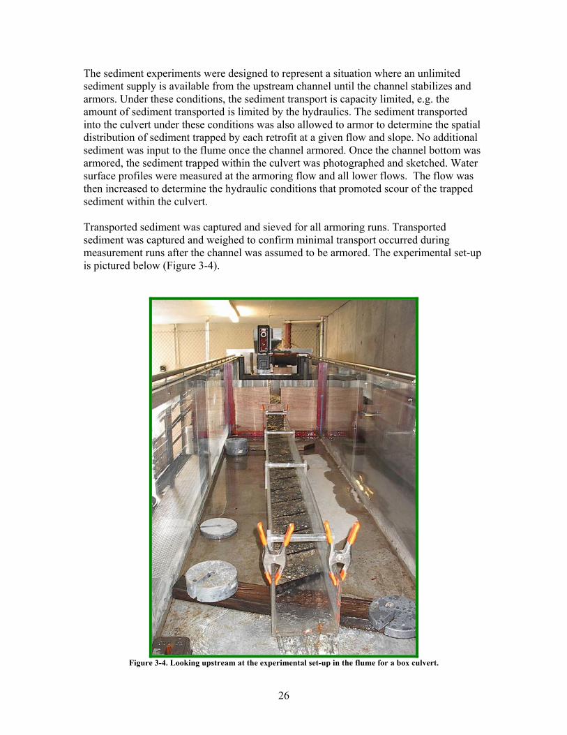
The sediment experiments were designed to represent a situation where an unlimited sediment supply is available from the upstream channel until the channel stabilizes and armors. Under these conditions, the sediment transport is capacity limited, e.g. the amount of sediment transported is limited by the hydraulics. The sediment transported into the culvert under these conditions was also allowed to armor to determine the spatial distribution of sediment trapped by each retrofit at a given flow and slope. No additional sediment was input to the flume once the channel armored. Once the channel bottom was armored, the sediment trapped within the culvert was photographed and sketched. Water surface profiles were measured at the armoring flow and all lower flows. The flow was then increased to determine the hydraulic conditions that promoted scour of the trapped sediment within the culvert. Transported sediment was captured and sieved for all armoring runs. Transported sediment was captured and weighed to confirm minimal transport occurred during measurement runs after the channel was assumed to be armored. The experimental set-up is pictured below (Figure 3-4).

Figure 3-4. Looking upstream at the experimental set-up in the flume for a box culvert.

26

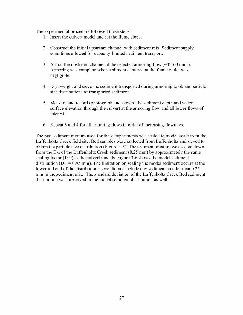
The experimental procedure followed these steps: 1. Insert the culvert model and set the flume slope.

2. Construct the initial upstream channel with sediment mix. Sediment supply

conditions allowed for capacity-limited sediment transport.

3. Armor the upstream channel at the selected armoring flow (~45-60 mins). Armoring was complete when sediment captured at the flume outlet was negligible.

4. Dry, weight and sieve the sediment transported during armoring to obtain particle size distributions of transported sediment.

5. Measure and record (photograph and sketch) the sediment depth and water surface elevation through the culvert at the armoring flow and all lower flows of interest.

6. Repeat 3 and 4 for all armoring flows in order of increasing flowrates.

The bed sediment mixture used for these experiments was scaled to model-scale from the Luffenholtz Creek field site. Bed samples were collected from Luffenholtz and sieved to obtain the particle size distribution (Figure 3-5). The sediment mixture was scaled down from the D50 of the Luffenholtz Creek sediment (8.25 mm) by approximately the same scaling factor (1: 9) as the culvert models. Figure 3-6 shows the model sediment distribution (D50 = 0.95 mm). The limitation on scaling the model sediment occurs at the lower tail end of the distribution as we did not include any sediment smaller than 0.25 mm in the sediment mix. The standard deviation of the Luffenholtz Creek Bed sediment distribution was preserved in the model sediment distribution as well.

27

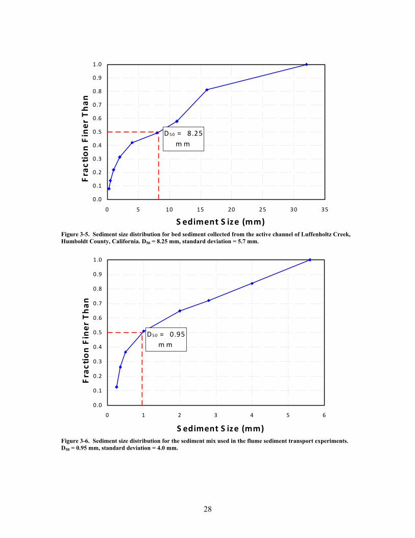
D50 =  8.25  mm      

0.0

0.1

0.2

0.3

0.4

0.5

0.6

0.7

0.8

0.9

1.0

0 5 10 15 20 25 30 35

S ediment S ize (mm)

Fraction Finer Than

Figure 3-5. Sediment size distribution for bed sediment collected from the active channel of Luffenholtz Creek, Humboldt County, California. D50 = 8.25 mm, standard deviation = 5.7 mm.

D50 =  0.95  mm

0.0

0.1

0.2

0.3

0.4

0.5

0.6

0.7

0.8

0.9

1.0

0 1 2 3 4 5 6

S ediment S ize (mm)

Fraction Finer Than

Figure 3-6. Sediment size distribution for the sediment mix used in the flume sediment transport experiments. D50 = 0.95 mm, standard deviation = 4.0 mm.

28

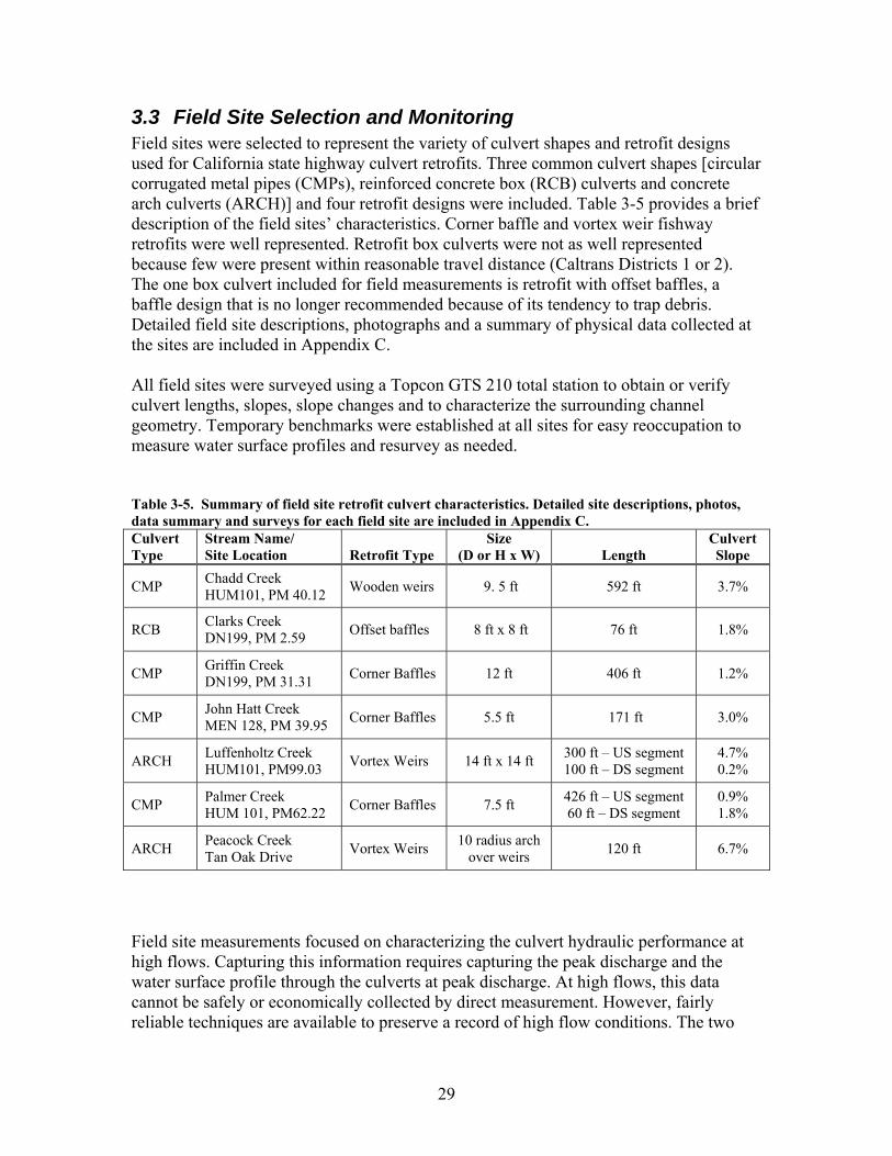
3.3 Field Site Selection and Monitoring Field sites were selected to represent the variety of culvert shapes and retrofit designs used for California state highway culvert retrofits. Three common culvert shapes [circular corrugated metal pipes (CMPs), reinforced concrete box (RCB) culverts and concrete arch culverts (ARCH)] and four retrofit designs were included. Table 3-5 provides a brief description of the field sites’ characteristics. Corner baffle and vortex weir fishway retrofits were well represented. Retrofit box culverts were not as well represented because few were present within reasonable travel distance (Caltrans Districts 1 or 2). The one box culvert included for field measurements is retrofit with offset baffles, a baffle design that is no longer recommended because of its tendency to trap debris. Detailed field site descriptions, photographs and a summary of physical data collected at the sites are included in Appendix C. All field sites were surveyed using a Topcon GTS 210 total station to obtain or verify culvert lengths, slopes, slope changes and to characterize the surrounding channel geometry. Temporary benchmarks were established at all sites for easy reoccupation to measure water surface profiles and resurvey as needed. Table 3-5. Summary of field site retrofit culvert characteristics. Detailed site descriptions, photos, data summary and surveys for each field site are included in Appendix C. Culvert Type

Stream Name/ Site Location Retrofit Type

Size (D or H x W) Length

Culvert Slope

CMP Chadd Creek HUM101, PM 40.12 Wooden weirs 9. 5 ft 592 ft 3.7%

RCB Clarks Creek DN199, PM 2.59 Offset baffles 8 ft x 8 ft 76 ft 1.8%

CMP Griffin Creek DN199, PM 31.31 Corner Baffles 12 ft 406 ft 1.2%

CMP John Hatt Creek MEN 128, PM 39.95 Corner Baffles 5.5 ft 171 ft 3.0%

ARCH Luffenholtz Creek HUM101, PM99.03 Vortex Weirs 14 ft x 14 ft 300 ft – US segment

100 ft – DS segment 4.7% 0.2%

CMP Palmer Creek HUM 101, PM62.22 Corner Baffles 7.5 ft 426 ft – US segment

60 ft – DS segment 0.9% 1.8%

ARCH Peacock Creek Tan Oak Drive Vortex Weirs 10 radius arch

over weirs 120 ft 6.7%

Field site measurements focused on characterizing the culvert hydraulic performance at high flows. Capturing this information requires capturing the peak discharge and the water surface profile through the culverts at peak discharge. At high flows, this data cannot be safely or economically collected by direct measurement. However, fairly reliable techniques are available to preserve a record of high flow conditions. The two

29

methods used for this study were installing peak stage recorders (PSRs) upstream of the culverts and marking the culvert barrels with transverse clay stripes at regular intervals through the culvert barrel (Figure 3-7 & Figure 3-8). The peak stage recorders use a floating substance (finely ground cork) that sticks to an internal lathe to mark the high water level (Figure 3-7b). The peak stage recorders are reset following major storms. The PSRs were located so that the peak stage measured corresponded to the culvert inlet headwater depth at peak discharge. As Figure 3-7a shows, the PSRs were constructed with surveying tape on the outside so that they also served as staff plates for the sites. In the culvert barrel, the clay stripes are washed off up to the high water mark leaving a record of the water surface profile through the culvert barrel that can be surveyed after the high flow recedes. A custom horizontal survey rod, level and target was constructed for surveying the bottom of the clay lines and each line was rated Good, Fair or Poor to indicate the quality of the measurement. The clay line locations and interval spacing varied for each culvert to capture water surface directly above and between the baffles. In addition to the peak stage recorders and clay stripes, a rating curve was developed for most of the sites so that discharge at peak stages could be estimated. Discharge measurements were collected over a range of flows using a magnetic Price AA (Rickly Hydrological, Model #6215) or a standard Pygmy meter (Model#6205) as appropriate for the conditions. Where rating curves could not be developed, site discharge measurements were computed multiple ways such as comparison to nearby gaged watersheds, using weir flow equations, or applying the channel slope-area method using surveyed high water marks. These techniques were also used to check rating curve high flow estimates. The project goal was to collect two complete water surface profiles (WSPs) at each field site. One WSP obtained at the peak discharge occurring during the study period, and the other an intermediate discharge that fully submerged the culvert retrofits by at least twice their maximum height. To efficiently allocate field crews and instruments, the sites were split into two subgroups with field efforts in year 1 (2005-2006) targeted at the first subgroup and year 2 (2006-2007) at the second. The first subgroup included Palmer, Luffenholtz, Peacock and Clarks creeks. Griffin, John Hatt and Chadd creeks were selected for intense study during 2006-2007. When the project was extended through June 2008 to conduct additional flume experiments, many of the field sites were also prepared for an additional season of measurements to take advantage of any additional high flows. Several higher flows than those experienced between October 2006 and May 2007 occurred in 2007 and 2008 so additional field measurements were collected at John Hatt, Chadd, Griffin and Clarks creeks.

30

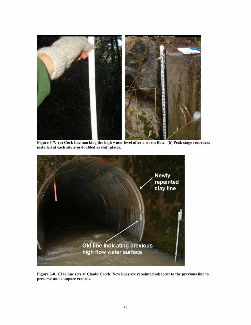
Figure 3-7. (a) Cork line marking the high water level after a storm flow. (b) Peak stage recorders installed at each site also doubled as staff plates.

Figure 3-8. Clay line sets at Chadd Creek. New lines are repainted adjacent to the previous line to preserve and compare records.

31

3.4 Laboratory and Field Data Analyses Computer models and empirical design equations are the primary tools for culvert design and analysis. The laboratory and field data collected over the course of the study were analyzed using all appropriate methods to demonstrate suitable approaches and applicable model assumptions. Culvert hydraulic models exist as stand-alone programs and culvert hydraulics modules have been incorporated into open channel flow models. The stand-alone models provide detailed analysis of the culvert inlet, outlet and barrel hydraulic performance and are the most common tool used in design of road culverts. The culvert hydraulics model generally used to design state highway culverts is HY-8 (FHWA, 2007), a public domain program developed by the Federal Highways Administration. Other models of this type include the public domain models FishXing (Furniss et al., 2006) and HydroCulv (Chanson, 1999), and the commercial software CulvertMaster (Haestad Methods). All of these models perform similar analyses of culvert hydraulics for standard culverts and simulation results compare well. FishXing is unique because, in addition to the culvert hydraulic simulations, it also incorporates fish swimming ability for direct analysis of fish passage. Open channel flow models that include a culvert analysis module allow engineers to evaluate the overall impacts of culvert design on a stream channel and the influence of channel conditions on culvert performance. The most commonly used model of this type is HEC-RAS (USACE, 2007). HEC-RAS is a one-dimensional, gradually-varied, open channel flow model that includes culvert hydraulics as an optional module. For analysis of the field and laboratory data collected during this study, HY-8 and HEC-RAS were used because these are the predominant hydraulic models used by Caltrans project engineers. FishXing V3.0 was also used to check analyses and to simulate laboratory experiments with flow rates below HY-8’s limit for significant figures. The laboratory experiments were simulated at the laboratory scale to determine laboratory-scale effective roughness values and water surface elevation profiles, and determine headloss coefficients for both the retrofit and non-retrofit model culverts. As presented in Section 2.3, several approaches that allow direct application of design equations or standard culvert hydraulic models have been used for the design and analysis of retrofit culverts including:

• Using the built-in culvert shapes and increasing the culvert material roughness to account for the presence of retrofits,

• Using an analysis model that allows a user-defined culvert shape and removing the area occupied by the retrofit, or

• Using a model’s embedded culvert option and embedding the culvert or culvert segments to the retrofit height.

32

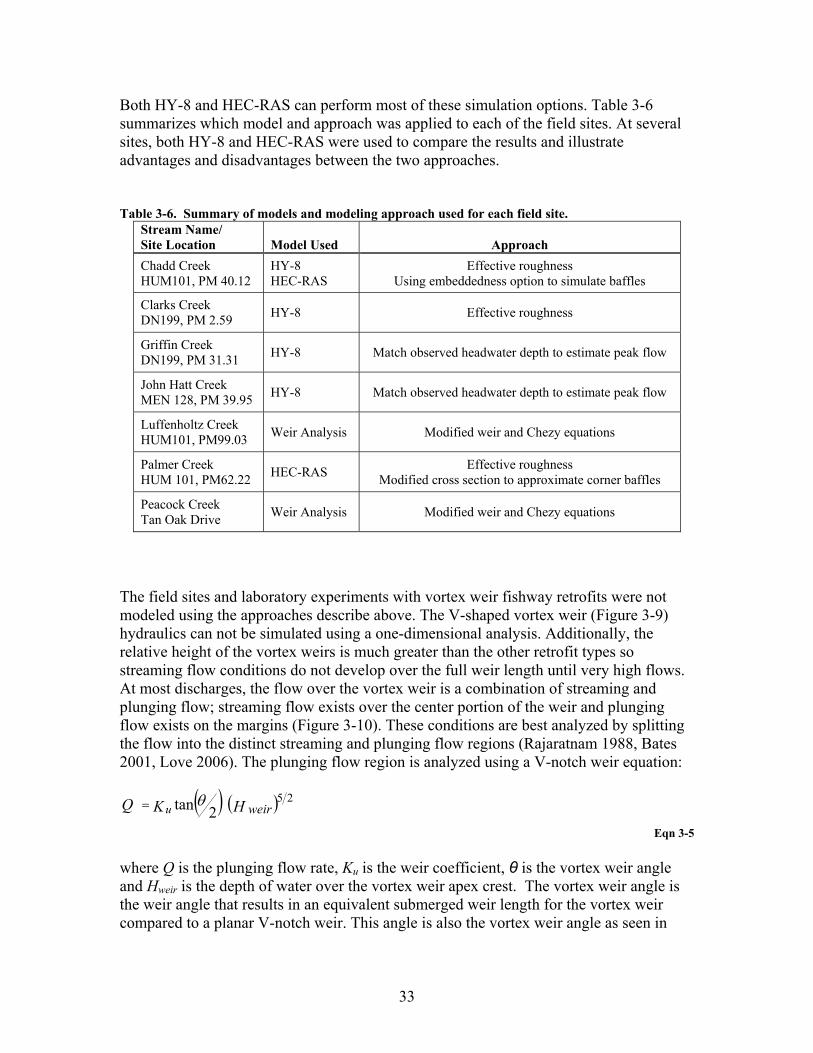
Both HY-8 and HEC-RAS can perform most of these simulation options. Table 3-6 summarizes which model and approach was applied to each of the field sites. At several sites, both HY-8 and HEC-RAS were used to compare the results and illustrate advantages and disadvantages between the two approaches. Table 3-6. Summary of models and modeling approach used for each field site.

Stream Name/ Site Location Model Used Approach Chadd Creek HUM101, PM 40.12

HY-8 HEC-RAS

Effective roughness Using embeddedness option to simulate baffles

Clarks Creek DN199, PM 2.59 HY-8 Effective roughness

Griffin Creek DN199, PM 31.31 HY-8 Match observed headwater depth to estimate peak flow

John Hatt Creek MEN 128, PM 39.95 HY-8 Match observed headwater depth to estimate peak flow

Luffenholtz Creek HUM101, PM99.03 Weir Analysis Modified weir and Chezy equations

Palmer Creek HUM 101, PM62.22 HEC-RAS Effective roughness

Modified cross section to approximate corner baffles

Peacock Creek Tan Oak Drive Weir Analysis Modified weir and Chezy equations

The field sites and laboratory experiments with vortex weir fishway retrofits were not modeled using the approaches describe above. The V-shaped vortex weir (Figure 3-9) hydraulics can not be simulated using a one-dimensional analysis. Additionally, the relative height of the vortex weirs is much greater than the other retrofit types so streaming flow conditions do not develop over the full weir length until very high flows. At most discharges, the flow over the vortex weir is a combination of streaming and plunging flow; streaming flow exists over the center portion of the weir and plunging flow exists on the margins (Figure 3-10). These conditions are best analyzed by splitting the flow into the distinct streaming and plunging flow regions (Rajaratnam 1988, Bates 2001, Love 2006). The plunging flow region is analyzed using a V-notch weir equation:

( ) ( )HKQ weiru25

2tan θ=

Eqn 3-5 where Q is the plunging flow rate, Ku is the weir coefficient, θ is the vortex weir angle and Hweir is the depth of water over the vortex weir apex crest. The vortex weir angle is the weir angle that results in an equivalent submerged weir length for the vortex weir compared to a planar V-notch weir. This angle is also the vortex weir angle as seen in

33

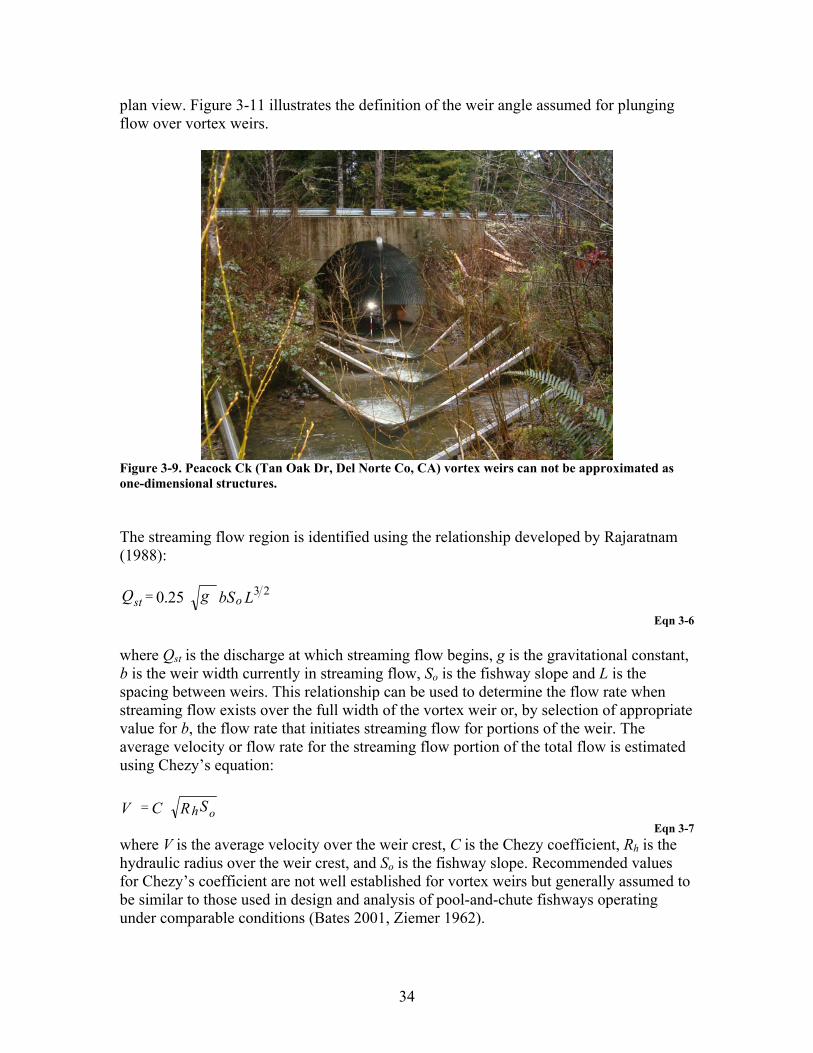
plan view. Figure 3-11 illustrates the definition of the weir angle assumed for plunging flow over vortex weirs.

Figure 3-9. Peacock Ck (Tan Oak Dr, Del Norte Co, CA) vortex weirs can not be approximated as one-dimensional structures. The streaming flow region is identified using the relationship developed by Rajaratnam (1988):

LbSgQ ost2325.0=

Eqn 3-6 where Qst is the discharge at which streaming flow begins, g is the gravitational constant, b is the weir width currently in streaming flow, So is the fishway slope and L is the spacing between weirs. This relationship can be used to determine the flow rate when streaming flow exists over the full width of the vortex weir or, by selection of appropriate value for b, the flow rate that initiates streaming flow for portions of the weir. The average velocity or flow rate for the streaming flow portion of the total flow is estimated using Chezy’s equation:

SRCV h o= Eqn 3-7

where V is the average velocity over the weir crest, C is the Chezy coefficient, Rh is the hydraulic radius over the weir crest, and So is the fishway slope. Recommended values for Chezy’s coefficient are not well established for vortex weirs but generally assumed to be similar to those used in design and analysis of pool-and-chute fishways operating under comparable conditions (Bates 2001, Ziemer 1962).

34

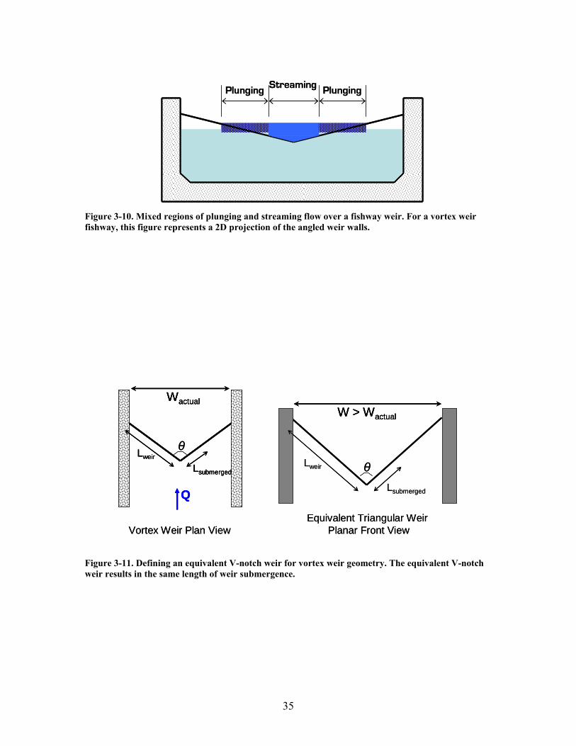
Plunging PlungingStreamingPlunging PlungingStreaming

Figure 3-10. Mixed regions of plunging and streaming flow over a fishway weir. For a vortex weir fishway, this figure represents a 2D projection of the angled weir walls. Wactual

Q

Vortex Weir Plan ViewEquivalent Triangular Weir

Planar Front View

W > Wactual

LweirLweir

Lsubmerged

Lsubmerged θ

θ

WactualWactual

QQ

Vortex Weir Plan ViewEquivalent Triangular Weir

Planar Front View

W > WactualW > Wactual

LweirLweirLweir

Lsubmerged

LsubmergedLsubmerged θ

θ

Figure 3-11. Defining an equivalent V-notch weir for vortex weir geometry. The equivalent V-notch weir results in the same length of weir submergence.

35

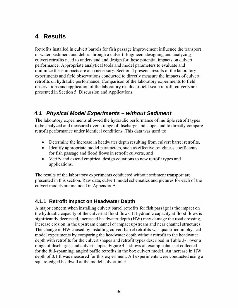
4 Results Retrofits installed in culvert barrels for fish passage improvement influence the transport of water, sediment and debris through a culvert. Engineers designing and analyzing culvert retrofits need to understand and design for these potential impacts on culvert performance. Appropriate analytical tools and model parameters to evaluate and minimize these impacts are also necessary. Section 4 presents results of the laboratory experiments and field observations conducted to directly measure the impacts of culvert retrofits on hydraulic performance. Comparison of the laboratory experiments to field observations and application of the laboratory results to field-scale retrofit culverts are presented in Section 5: Discussion and Applications.

4.1 Physical Model Experiments – without Sediment The laboratory experiments allowed the hydraulic performance of multiple retrofit types to be analyzed and measured over a range of discharge and slope, and to directly compare retrofit performance under identical conditions. This data was used to:

• Determine the increase in headwater depth resulting from culvert barrel retrofits, • Identify appropriate model parameters, such as effective roughness coefficients,

for fish passage and flood flows in retrofit culverts, and • Verify and extend empirical design equations to new retrofit types and

applications. The results of the laboratory experiments conducted without sediment transport are presented in this section. Raw data, culvert model schematics and pictures for each of the culvert models are included in Appendix A.

4.1.1 Retrofit Impact on Headwater Depth A major concern when installing culvert barrel retrofits for fish passage is the impact on the hydraulic capacity of the culvert at flood flows. If hydraulic capacity at flood flows is significantly decreased, increased headwater depth (HW) may damage the road crossing, increase erosion in the upstream channel or impact upstream and near channel structures. The change in HW caused by installing culvert barrel retrofits was quantified in physical model experiments by comparing the headwater depth without retrofit to the headwater depth with retrofits for the culvert shapes and retrofit types described in Table 3-1 over a range of discharges and culvert slopes. Figure 4-1 shows an example data set collected for the full-spanning, angled baffle retrofits in the box culvert model. An increase in HW depth of 0.1 ft was measured for this experiment. All experiments were conducted using a square-edged headwall at the model culvert inlet.

36

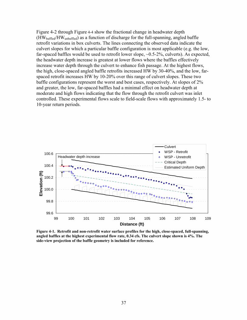
Figure 4-2 through Figure 4-4 show the fractional change in headwater depth (HWbaffled/HWunbaffled) as a function of discharge for the full-spanning, angled baffle retrofit variations in box culverts. The lines connecting the observed data indicate the culvert slopes for which a particular baffle configuration is most applicable (e.g. the low, far-spaced baffles would be used to retrofit lower slope, ~0.5-2%, culverts). As expected, the headwater depth increase is greatest at lower flows where the baffles effectively increase water depth through the culvert to enhance fish passage. At the highest flows, the high, close-spaced angled baffle retrofits increased HW by 30-40%, and the low, far-spaced retrofit increases HW by 10-20% over this range of culvert slopes. These two baffle configurations represent the worst and best cases, respectively. At slopes of 2% and greater, the low, far-spaced baffles had a minimal effect on headwater depth at moderate and high flows indicating that the flow through the retrofit culvert was inlet controlled. These experimental flows scale to field-scale flows with approximately 1.5- to 10-year return periods.

99.6

99.8

100.0

100.2

100.4

100.6

99 100 101 102 103 104 105 106 107 108 109Distance (ft)

Elev

atio

n (ft

)

CulvertWSP - RetrofitWSP - UnretrofitCritical DepthEstimated Uniform Depth

Headwater depth increase

Figure 4-1. Retrofit and non-retrofit water surface profiles for the high, close-spaced, full-spanning, angled baffles at the highest experimental flow rate, 0.34 cfs. The culvert slope shown is 4%. The side-view projection of the baffle geometry is included for reference.

37

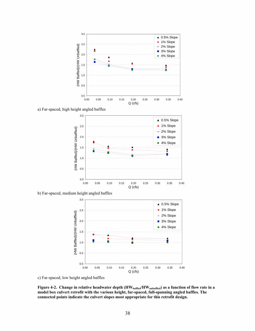
0.0

0.5

1.0

1.5

2.0

2.5

3.0

0.00 0.05 0.10 0.15 0.20 0.25 0.30 0.35 0.40Q (cfs)

(HW

Baf

fled)

/(HW

Unb

affle

d)

0.5% Slope1% Slope2% Slope3% Slope4% Slope

a) Far-spaced, high height angled baffles

0.0

0.5

1.0

1.5

2.0

2.5

3.0

0.00 0.05 0.10 0.15 0.20 0.25 0.30 0.35 0.40Q (cfs)

(HW

Baf

fled)

/(HW

Unb

affle

d)

0.5% Slope1% Slope

2% Slope3% Slope

4% Slope

b) Far-spaced, medium height angled baffles

0.0

0.5

1.0

1.5

2.0

2.5

3.0

0.00 0.05 0.10 0.15 0.20 0.25 0.30 0.35 0.40Q (cfs)

(HW

Baf

fled)

/(HW

Unb

affle

d)

0.5% Slope1% Slope

2% Slope3% Slope

4% Slope

c) Far-spaced, low height angled baffles Figure 4-2. Change in relative headwater depth (HWbaffled/HWunbaffled) as a function of flow rate in a model box culvert retrofit with the various height, far-spaced, full-spanning angled baffles. The connected points indicate the culvert slopes most appropriate for this retrofit design.

38

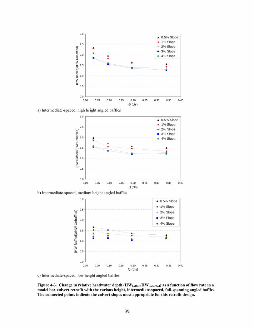
0.0

0.5

1.0

1.5

2.0

2.5

3.0

0.00 0.05 0.10 0.15 0.20 0.25 0.30 0.35 0.40Q (cfs)

(HW

Baf

fled)

/(HW

Unb

affle

d)

0.5% Slope1% Slope2% Slope3% Slope4% Slope

a) Intermediate-spaced, high height angled baffles

0.0

0.5

1.0

1.5

2.0

2.5

3.0

0.00 0.05 0.10 0.15 0.20 0.25 0.30 0.35 0.40Q (cfs)

(HW

Baf

fled)

/(HW

Unb

affle

d)

0.5% Slope1% Slope2% Slope3% Slope4% Slope

b) Intermediate-spaced, medium height angled baffles

0.0

0.5

1.0

1.5

2.0

2.5

3.0

0.00 0.05 0.10 0.15 0.20 0.25 0.30 0.35 0.40Q (cfs)

(HW

Baf

fled)

/(HW

Unb

affle

d)

0.5% Slope1% Slope

2% Slope3% Slope

4% Slope

c) Intermediate-spaced, low height angled baffles Figure 4-3. Change in relative headwater depth (HWbaffled/HWunbaffled) as a function of flow rate in a model box culvert retrofit with the various height, intermediate-spaced, full-spanning angled baffles. The connected points indicate the culvert slopes most appropriate for this retrofit design.

39

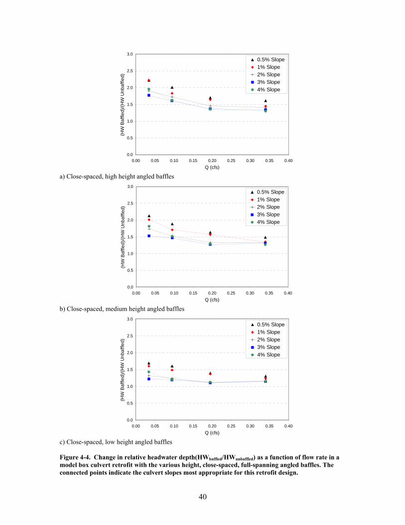
0.0

0.5

1.0

1.5

2.0

2.5

3.0

0.00 0.05 0.10 0.15 0.20 0.25 0.30 0.35 0.40Q (cfs)

(HW

Baf

fled)

/(HW

Unb

affle

d)

0.5% Slope1% Slope2% Slope3% Slope4% Slope

a) Close-spaced, high height angled baffles

0.0

0.5

1.0

1.5

2.0

2.5

3.0

0.00 0.05 0.10 0.15 0.20 0.25 0.30 0.35 0.40Q (cfs)

(HW

Baf

fled)

/(HW

Unb

affle

d)

0.5% Slope1% Slope2% Slope3% Slope4% Slope

b) Close-spaced, medium height angled baffles

0.0

0.5

1.0

1.5

2.0

2.5

3.0

0.00 0.05 0.10 0.15 0.20 0.25 0.30 0.35 0.40Q (cfs)

(HW

Baf

fled)

/(HW

Unb

affle

d)

0.5% Slope1% Slope2% Slope3% Slope4% Slope

c) Close-spaced, low height angled baffles Figure 4-4. Change in relative headwater depth(HWbaffled/HWunbaffled) as a function of flow rate in a model box culvert retrofit with the various height, close-spaced, full-spanning angled baffles. The connected points indicate the culvert slopes most appropriate for this retrofit design.

40

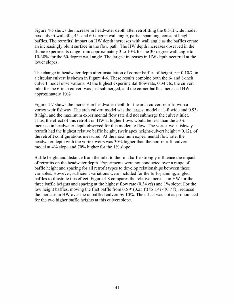
Figure 4-5 shows the increase in headwater depth after retrofitting the 0.5-ft wide model box culvert with 30-, 45- and 60-degree wall angle, partial spanning, constant height baffles. The retrofits’ impact on HW depth increases with wall angle as the baffles create an increasingly blunt surface in the flow path. The HW depth increases observed in the flume experiments range from approximately 3 to 10% for the 30-degree wall angle to 10-30% for the 60-degree wall angle. The largest increases in HW depth occurred at the lower slopes. The change in headwater depth after installation of corner baffles of height, z = 0.10D, in a circular culvert is shown in Figure 4-6. These results combine both the 6- and 8-inch culvert model observations. At the highest experimental flow rate, 0.34 cfs, the culvert inlet for the 6-inch culvert was just submerged, and the corner baffles increased HW approximately 10%. Figure 4-7 shows the increase in headwater depth for the arch culvert retrofit with a vortex weir fishway. The arch culvert model was the largest model at 1-ft wide and 0.93-ft high, and the maximum experimental flow rate did not submerge the culvert inlet. Thus, the effect of this retrofit on HW at higher flows would be less than the 50% increase in headwater depth observed for this moderate flow. The vortex weir fishway retrofit had the highest relative baffle height, (weir apex height/culvert height = 0.12), of the retrofit configurations measured. At the maximum experimental flow rate, the headwater depth with the vortex weirs was 30% higher than the non-retrofit culvert model at 4% slope and 70% higher for the 1% slope. Baffle height and distance from the inlet to the first baffle strongly influence the impact of retrofits on the headwater depth. Experiments were not conducted over a range of baffle height and spacing for all retrofit types to develop relationships between these variables. However, sufficient variations were included for the full-spanning, angled baffles to illustrate this effect. Figure 4-8 compares the relative increase in HW for the three baffle heights and spacing at the highest flow rate (0.34 cfs) and 1% slope. For the low height baffles, moving the first baffle from 0.5W (0.25 ft) to 1.4W (0.7 ft), reduced the increase in HW over the unbaffled culvert by 10%. The effect was not as pronounced for the two higher baffle heights at this culvert slope.

41

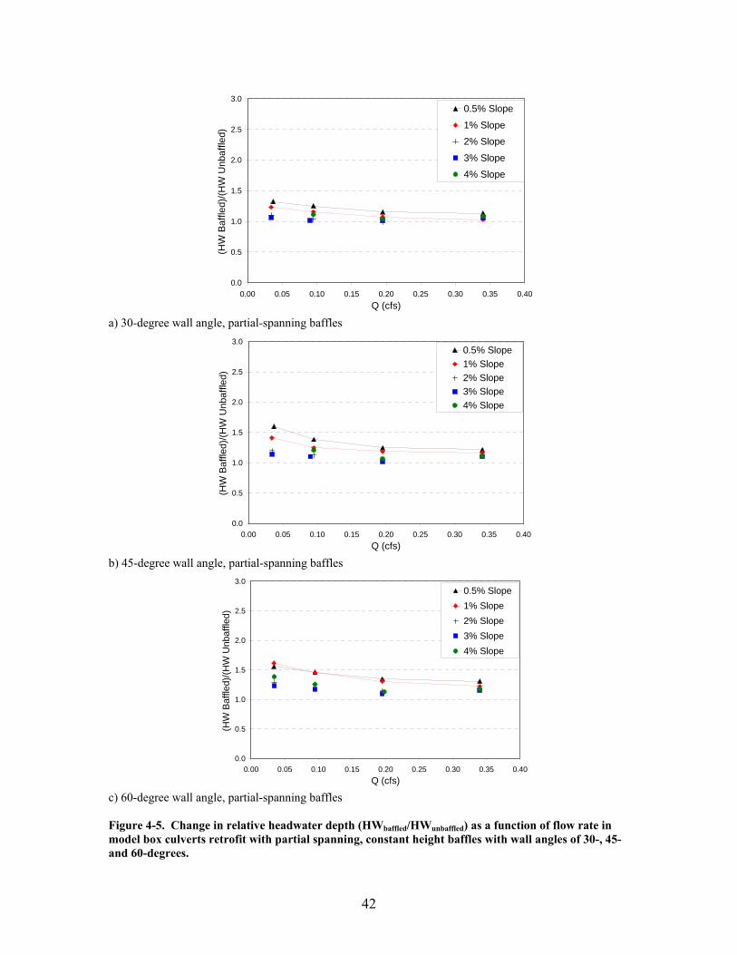
0.0

0.5

1.0

1.5

2.0

2.5

3.0

0.00 0.05 0.10 0.15 0.20 0.25 0.30 0.35 0.40Q (cfs)

(HW

Baf

fled)

/(HW

Unb

affle

d)

0.5% Slope

1% Slope

2% Slope

3% Slope

4% Slope

a) 30-degree wall angle, partial-spanning baffles

0.0

0.5

1.0

1.5

2.0

2.5

3.0

0.00 0.05 0.10 0.15 0.20 0.25 0.30 0.35 0.40Q (cfs)

(HW

Baf

fled)

/(HW

Unb

affle

d)

0.5% Slope1% Slope2% Slope3% Slope4% Slope

b) 45-degree wall angle, partial-spanning baffles

0.0

0.5

1.0

1.5

2.0

2.5

3.0

0.00 0.05 0.10 0.15 0.20 0.25 0.30 0.35 0.40Q (cfs)

(HW

Baf

fled)

/(HW

Unb

affle

d)

0.5% Slope1% Slope2% Slope3% Slope4% Slope

c) 60-degree wall angle, partial-spanning baffles Figure 4-5. Change in relative headwater depth (HWbaffled/HWunbaffled) as a function of flow rate in model box culverts retrofit with partial spanning, constant height baffles with wall angles of 30-, 45- and 60-degrees.

42

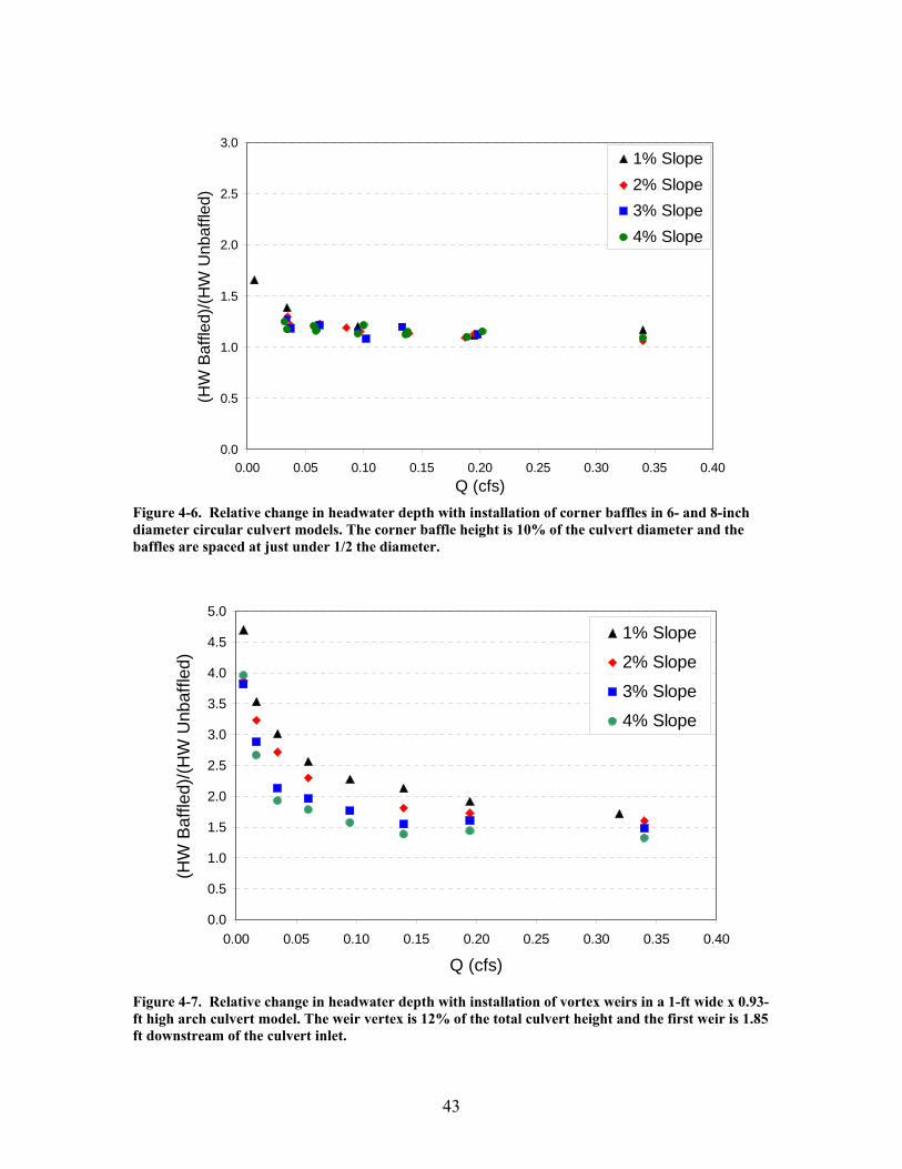
0.0

0.5

1.0

1.5

2.0

2.5

3.0

0.00 0.05 0.10 0.15 0.20 0.25 0.30 0.35 0.40Q (cfs)

(HW

Baf

fled)

/(HW

Unb

affle

d)

1% Slope2% Slope3% Slope4% Slope

Figure 4-6. Relative change in headwater depth with installation of corner baffles in 6- and 8-inch diameter circular culvert models. The corner baffle height is 10% of the culvert diameter and the baffles are spaced at just under 1/2 the diameter.

0.0

0.5

1.0

1.5

2.0

2.5

3.0

3.5

4.0

4.5

5.0

0.00 0.05 0.10 0.15 0.20 0.25 0.30 0.35 0.40

Q (cfs)

(HW

Baf

fled)

/(HW

Unb

affle

d)

1% Slope

2% Slope

3% Slope

4% Slope

Figure 4-7. Relative change in headwater depth with installation of vortex weirs in a 1-ft wide x 0.93-ft high arch culvert model. The weir vertex is 12% of the total culvert height and the first weir is 1.85 ft downstream of the culvert inlet.

43

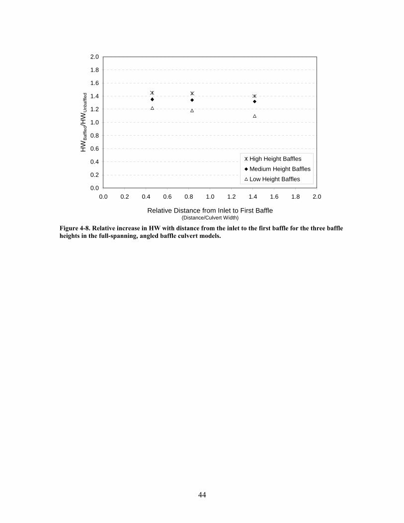
0.0

0.2

0.4

0.6

0.8

1.0

1.2

1.4

1.6

1.8

2.0

0.0 0.2 0.4 0.6 0.8 1.0 1.2 1.4 1.6 1.8 2.0

Relative Distance from Inlet to First Baffle (Distance/Culvert Width)

HW

Baffl

ed/H

WU

nbaf

fled

High Height Baffles

Medium Height Baffles

Low Height Baffles

Figure 4-8. Relative increase in HW with distance from the inlet to the first baffle for the three baffle heights in the full-spanning, angled baffle culvert models.

44

4.1.2 Laboratory-Scale Retrofit Culvert Effective Roughness At discharges that fully submerge the installed baffles or weirs, the main flow of water through the culvert streams over the top of the retrofits. Under these streaming flow conditions, the retrofits act as roughness elements and their influence on the culvert hydraulics can be quantified using a roughness parameter such as Manning’s n or Darcy’s friction factor, f. Identifying effective roughness parameters for a particular retrofit design allows direct application of common culvert hydraulic models to predict hydraulic performance of retrofit culverts under streaming flow conditions. Because most of the commonly used hydraulic models expect roughness expressed as n for input, the roughness coefficients are presented here as Manning’s n values. These values could easily be converted to equivalent friction factors or other similar coefficients using standard conversion equations. The effective roughness approach assumes streaming flow conditions, so it may not be applicable for all retrofit configurations. Retrofits designed to perform solely or partially as weirs over a wide range of flow, such as the vortex weirs, do not meet the streaming flow assumption. For this reason, effective roughness coefficients were not determined for the vortex weir fishway retrofit or for experiments with average flow depth that did not fully submerge the baffles. Results and analysis of the vortex weir retrofits are presented separately in Section 4.3. Additionally, the effective roughness values presented in this section apply only to the laboratory-scale model culverts. Section 5.1.2 describes application of the experimental results to field conditions and provides examples of using these results in design and analysis of field-scale culverts. Figure 4-9 through Figure show the effective roughness versus relative submergence (water depth/maximum baffle height) for the full-spanning box culvert angled baffle retrofit designs. As expected, the effective roughness decreases with increasing baffle submergence, and each baffle configuration approaches a characteristic high flow roughness value. Figure 4-12 summarizes the effective roughness coefficients for all baffle configurations and culvert slopes over the range of experimental flow rates. The multiple points included for each baffle configuration are the different culvert slopes.

45

0.000

0.020

0.040

0.060

0.080

0.100

0.120

0.0 1.0 2.0 3.0 4.0 5.0 6.0 7.0 8.0 9.0 10.0Water Depth/Baffle Height

Rou

ghne

ss C

oef (

n)

0.5% Slope

1% Slope

2% Slope

3% Slope

4% Slope

a) Far-spaced, high height angled baffles

0.000

0.020

0.040

0.060

0.080

0.100

0.120

0.0 1.0 2.0 3.0 4.0 5.0 6.0 7.0 8.0 9.0 10.0Water Depth/Baffle Height

Rou

ghne

ss C

oef (

n)

0.5% Slope

1% Slope

2% Slope

3% Slope

4% Slope

b) Far-spaced, medium height angled baffles

0.000

0.020

0.040

0.060

0.080

0.100

0.120

0.0 1.0 2.0 3.0 4.0 5.0 6.0 7.0 8.0 9.0 10.0Water Depth/Baffle Height

Rou

ghne

ss C

oef (

n)

0.5% Slope

1% Slope

2% Slope

3% Slope

4% Slope

c) Far-spaced, low height angled baffles Figure 4-9. Laboratory-scale effective roughness (as Manning’s n) versus relative submergence (water depth / maximum baffle height) for various height, far-spaced, full-spanning angled baffles.

46

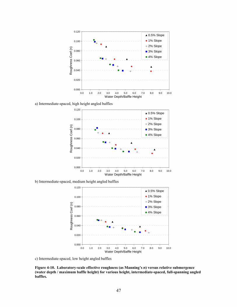
0.000

0.020

0.040

0.060

0.080

0.100

0.120

0.0 1.0 2.0 3.0 4.0 5.0 6.0 7.0 8.0 9.0 10.0Water Depth/Baffle Height

Rou

ghne

ss C

oef (

n)

0.5% Slope

1% Slope

2% Slope

3% Slope

4% Slope

a) Intermediate-spaced, high height angled baffles

0.000

0.020

0.040

0.060

0.080

0.100

0.120

0.0 1.0 2.0 3.0 4.0 5.0 6.0 7.0 8.0 9.0 10.0Water Depth/Baffle Height

Rou

ghne

ss C

oef (

n)

0.5% Slope

1% Slope

2% Slope

3% Slope

4% Slope

b) Intermediate-spaced, medium height angled baffles

0.000

0.020

0.040

0.060

0.080

0.100

0.120

0.0 1.0 2.0 3.0 4.0 5.0 6.0 7.0 8.0 9.0 10.0Water Depth/Baffle Height

Rou

ghne

ss C

oef (

n)

0.5% Slope

1% Slope

2% Slope

3% Slope

4% Slope

c) Intermediate-spaced, low height angled baffles Figure 4-10. Laboratory-scale effective roughness (as Manning’s n) versus relative submergence (water depth / maximum baffle height) for various height, intermediate-spaced, full-spanning angled baffles.

47

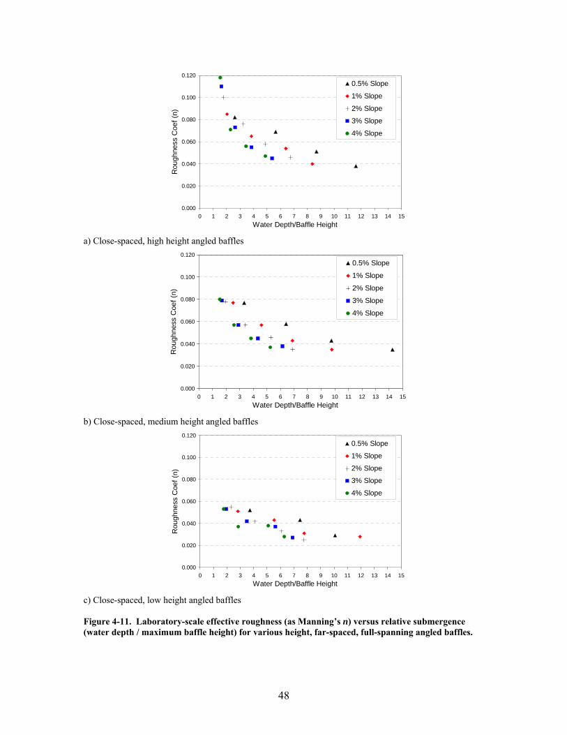
0.000

0.020

0.040

0.060

0.080

0.100

0.120

0 1 2 3 4 5 6 7 8 9 10 11 12 13 14 15Water Depth/Baffle Height

Rou

ghne

ss C

oef (

n)

0.5% Slope

1% Slope

2% Slope

3% Slope

4% Slope

a) Close-spaced, high height angled baffles

0.000

0.020

0.040

0.060

0.080

0.100

0.120

0 1 2 3 4 5 6 7 8 9 10 11 12 13 14 15Water Depth/Baffle Height

Rou

ghne

ss C

oef (

n)

0.5% Slope

1% Slope

2% Slope

3% Slope

4% Slope

b) Close-spaced, medium height angled baffles

0.000

0.020

0.040

0.060

0.080

0.100

0.120

0 1 2 3 4 5 6 7 8 9 10 11 12 13 14 15Water Depth/Baffle Height

Rou

ghne

ss C

oef (

n)

0.5% Slope

1% Slope

2% Slope

3% Slope

4% Slope

c) Close-spaced, low height angled baffles Figure 4-11. Laboratory-scale effective roughness (as Manning’s n) versus relative submergence (water depth / maximum baffle height) for various height, far-spaced, full-spanning angled baffles.

48

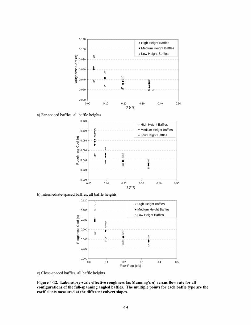
0.000

0.020

0.040

0.060

0.080

0.100

0.120

0.00 0.10 0.20 0.30 0.40 0.50Q (cfs)

Rou

ghne

ss C

oef (

n)

High Height BafflesMedium Height BafflesLow Height Baffles

a) Far-spaced baffles, all baffle heights

0.000

0.020

0.040

0.060

0.080

0.100

0.120

0.00 0.10 0.20 0.30 0.40 0.50Q (cfs)

Rou

ghne

ss C

oef (

n)

High Height BafflesMedium Height BafflesLow Height Baffles

b) Intermediate-spaced baffles, all baffle heights

0.000

0.020

0.040

0.060

0.080

0.100

0.120

0.0 0.1 0.2 0.3 0.4 0.5Flow Rate (cfs)

Rou

ghne

ss C

oef (

n)

High Height Baffles

Medium Height Baffles

Low Height Baffles

c) Close-spaced baffles, all baffle heights Figure 4-12. Laboratory-scale effective roughness (as Manning’s n) versus flow rate for all configurations of the full-spanning angled baffles. The multiple points for each baffle type are the coefficients measured at the different culvert slopes.

49

The effective roughness coefficients for the partial spanning, constant height angle baffles are presented in Figure 4-13 as a function of submergence ratio. The 30-degree wall angle baffle creates the lowest average flow depth; thus, has the lowest effective roughness coefficients with values ranging from 0.011 to 0.017 compared to a roughness of 0.008 for the unbaffled plexiglass model. The 45- and 60-degree wall angle baffles had laboratory-scale effective roughnesses of 0.013-0.020 and 0.015-0.025, respectively. Figure 4-14 summarizes the effective roughness for these models as a function of flow rate. As wall angle increases, the roughness increases as the surface obstructing the flow becomes increasingly blunt. Effective roughness approximately doubles for a wall angle increase from 30- to 60-degrees. Effective roughness coefficients as a function of baffle submergence for the circular culvert with corner baffle retrofits are shown in Figure 4-15. These results combine the 6- and 8-inch culvert models with the higher submergence ratios collected only from the 6-inch model. Again, the roughness coefficient varies strongly with submergence depth. High flow effective roughness values on the order of 0.020 would apply for the model retrofit culvert compared to 0.010 for the non-retrofit culvert model.

50

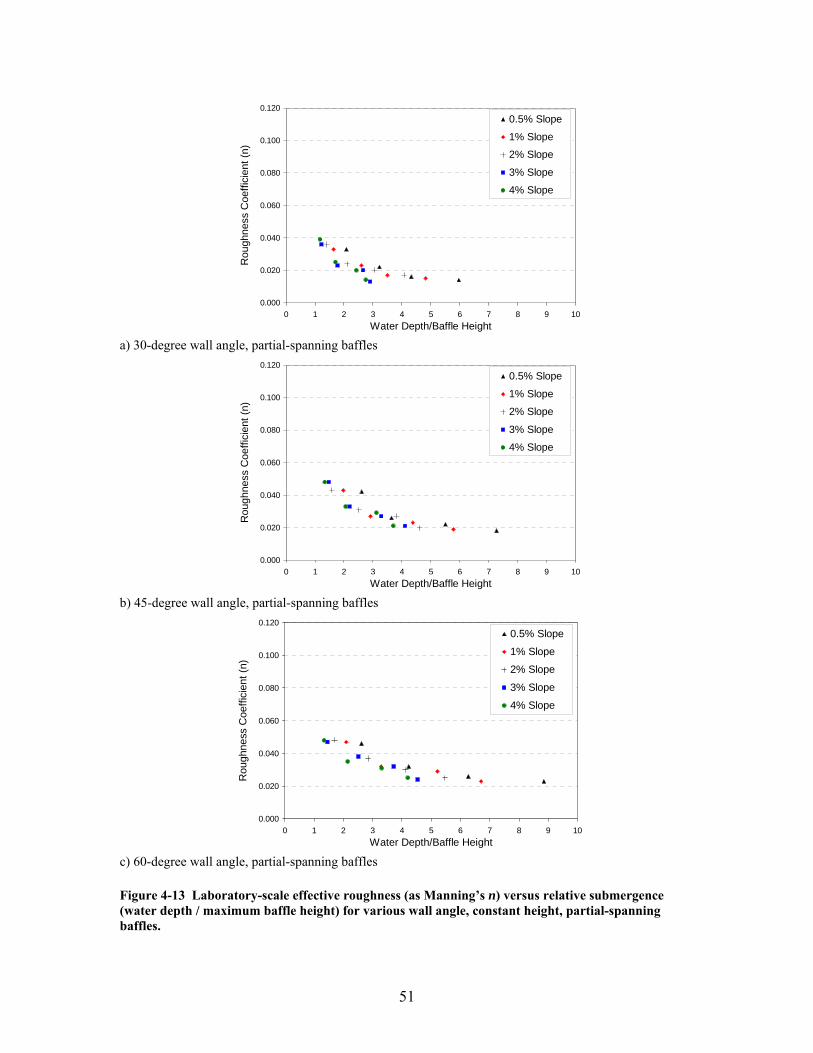
0.000

0.020

0.040

0.060

0.080

0.100

0.120

0 1 2 3 4 5 6 7 8 9 10Water Depth/Baffle Height

Rou

ghne

ss C

oeffi

cien

t (n)

0.5% Slope

1% Slope

2% Slope

3% Slope

4% Slope

a) 30-degree wall angle, partial-spanning baffles

0.000

0.020

0.040

0.060

0.080

0.100

0.120

0 1 2 3 4 5 6 7 8 9 10Water Depth/Baffle Height

Rou

ghne

ss C

oeffi

cien

t (n)

0.5% Slope

1% Slope

2% Slope

3% Slope

4% Slope

b) 45-degree wall angle, partial-spanning baffles

0.000

0.020

0.040

0.060

0.080

0.100

0.120

0 1 2 3 4 5 6 7 8 9 10Water Depth/Baffle Height

Rou

ghne

ss C

oeffi

cien

t (n)

0.5% Slope

1% Slope

2% Slope

3% Slope

4% Slope

c) 60-degree wall angle, partial-spanning baffles Figure 4-13 Laboratory-scale effective roughness (as Manning’s n) versus relative submergence (water depth / maximum baffle height) for various wall angle, constant height, partial-spanning baffles.

51

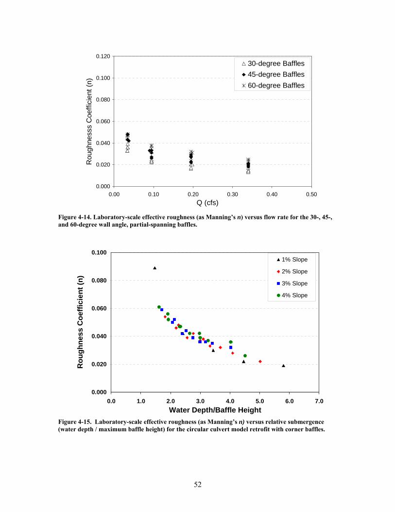
0.000

0.020

0.040

0.060

0.080

0.100

0.120

0.00 0.10 0.20 0.30 0.40 0.50Q (cfs)

Rou

ghne

sss

Coe

ffici

ent (

n)

30-degree Baffles45-degree Baffles60-degree Baffles

Figure 4-14. Laboratory-scale effective roughness (as Manning’s n) versus flow rate for the 30-, 45-, and 60-degree wall angle, partial-spanning baffles.

0.000

0.020

0.040

0.060

0.080

0.100

0.0 1.0 2.0 3.0 4.0 5.0 6.0 7.0Water Depth/Baffle Height

Rou

ghne

ss C

oeffi

cien

t (n)

1% Slope

2% Slope

3% Slope

4% Slope

Figure 4-15. Laboratory-scale effective roughness (as Manning’s n) versus relative submergence (water depth / maximum baffle height) for the circular culvert model retrofit with corner baffles.

52

4.1.3 Extension of Empirical Models As described previously (Section 2.1.1), the empirical equations developed by Rajaratnam, Katapodis and colleagues (Rajaratnam and Katapodis 1990; Rajaratnam et al. 1988, 1989, 1990, 1991) have been frequently used in the design and analysis of retrofit circular culverts. The application of these equations and extension of this approach to retrofit box culverts is presented in Section 3.1. The resulting dimensionless

equations ( )DyCDgSQQ oa

o 5

* == (Eqn 3-2) for circular culverts and

( zyCWgSQQ oa

o max 5

* == ) (Eqn 3-4) for box culverts were fit to the experimental data to determine the equation parameters C and a for the various culvert retrofits evaluated in this study. Figures 4-16 through 4-18 show the fit of the flume experiment data to Eqn 3-4 for the three heights and spacings used in the full-spanning angled baffle retrofit culvert models. These parameter values were determined using the maximum baffle height, zmax, as the scaling factor for the water depth, yo. The low, far-spaced baffle configuration approximates the minimum height and maximum spacing, and the high, close-spaced baffle configuration represents the maximum height and minimum spacing likely to be installed for fish passage improvement. Thus, the C and a values for these two baffle configurations can be interpreted as approximate upper and lower bounds for use in the design equations. The C and a values for additional baffle configurations fall between these extreme values. Figure 4-19 summarizes how C and a vary with baffle height and baffle spacing for the full-spanning, angled baffles. Both parameters vary with baffle spacing and height, but the magnitude of change is greater for C. The far baffle spacing parameters appear to vary differently than the intermediate and close spacing, as shown most clearly in Figure 4-19 b). This result is not unexpected as the far baffle spacing is the configuration least likely to maintain streaming flow conditions.

53

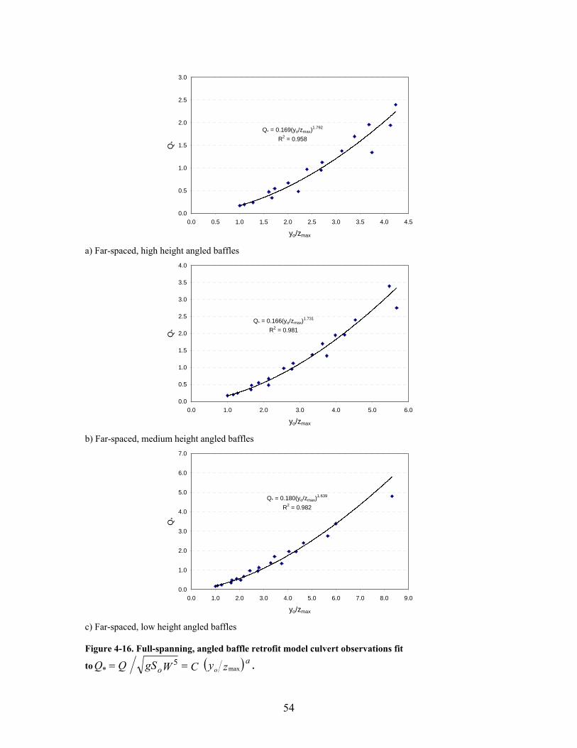
Q* = 0.169(yo/zmax)1.792

R2 = 0.958

0.0

0.5

1.0

1.5

2.0

2.5

3.0

0.0 0.5 1.0 1.5 2.0 2.5 3.0 3.5 4.0 4.5

yo/zmax

Q*

a) Far-spaced, high height angled baffles

Q* = 0.166(yo/zmax)1.731

R2 = 0.981

0.0

0.5

1.0

1.5

2.0

2.5

3.0

3.5

4.0

0.0 1.0 2.0 3.0 4.0 5.0 6.0

yo/zmax

Q*

b) Far-spaced, medium height angled baffles

Q* = 0.180(yo/zmax)1.639

R2 = 0.982

0.0

1.0

2.0

3.0

4.0

5.0

6.0

7.0

0.0 1.0 2.0 3.0 4.0 5.0 6.0 7.0 8.0 9.0

yo/zmax

Q*

c) Far-spaced, low height angled baffles Figure 4-16. Full-spanning, angled baffle retrofit model culvert observations fit

to ( )zyCWgSQQ oa

o max 5

* == .

54

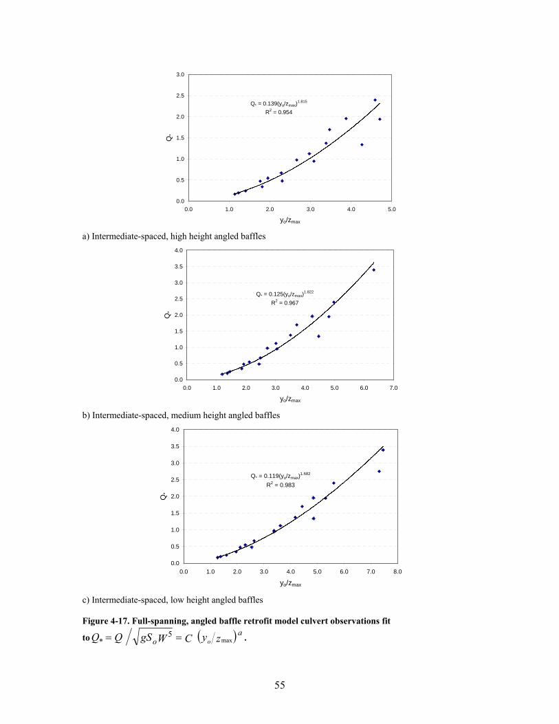
Q* = 0.139(yo/zmax)1.815

R2 = 0.954

0.0

0.5

1.0

1.5

2.0

2.5

3.0

0.0 1.0 2.0 3.0 4.0 5.0

yo/zmax

Q*

a) Intermediate-spaced, high height angled baffles

Q* = 0.125(yo/zmax)1.822

R2 = 0.967

0.0

0.5

1.0

1.5

2.0

2.5

3.0

3.5

4.0

0.0 1.0 2.0 3.0 4.0 5.0 6.0 7.0

yo/zmax

Q*

b) Intermediate-spaced, medium height angled baffles

Q* = 0.119(yo/zmax)1.682

R2 = 0.983

0.0

0.5

1.0

1.5

2.0

2.5

3.0

3.5

4.0

0.0 1.0 2.0 3.0 4.0 5.0 6.0 7.0 8.0

yo/zmax

Q*

c) Intermediate-spaced, low height angled baffles Figure 4-17. Full-spanning, angled baffle retrofit model culvert observations fit

to ( )zyCWgSQQ oa

o max 5

* == .

55

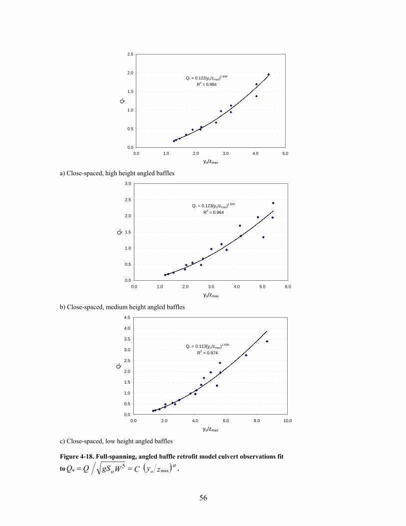
Q* = 0.122(yo/zmax)1.849

R2 = 0.984

0.0

0.5

1.0

1.5

2.0

2.5

0.0 1.0 2.0 3.0 4.0 5.0

yo/zmax

Q*

a) Close-spaced, high height angled baffles

Q* = 0.123(yo/zmax)1.695

R2 = 0.964

0.0

0.5

1.0

1.5

2.0

2.5

3.0

0.0 1.0 2.0 3.0 4.0 5.0 6

yo/zmax

Q*

.0

b) Close-spaced, medium height angled baffles

Q* = 0.113(yo/zmax)1.636

R2 = 0.974

0.0

0.5

1.0

1.5

2.0

2.5

3.0

3.5

4.0

4.5

0.0 2.0 4.0 6.0 8.0 10.0

yo/zmax

Q*

c) Close-spaced, low height angled baffles Figure 4-18. Full-spanning, angled baffle retrofit model culvert observations fit

to ( )zyCWgSQQ oa

o max 5

* == .

56

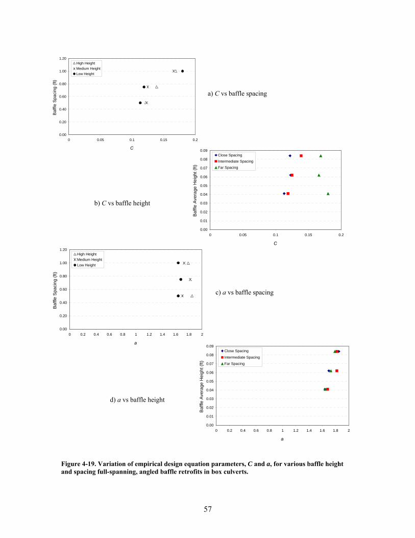
a) C vs baffle spacing

b) C vs baffle height

c) a vs baffle spacing

d) a vs baffle height Figure 4-19. Variation of empirical design equation parameters, C and a, for various baffle height and spacing full-spanning, angled baffle retrofits in box culverts.

0.00

0.20

0.40

0.60

0.80

1.00

1.20

0 0.05 0.1 0.15 0.2

C

Baffl

e Sp

acin

g (ft

)

High HeightMedium HeightLow Height

0.00

0.01

0.02

0.03

0.04

0.05

0.06

0.07

0.08

0.09

0 0.05 0.1 0.15 0.2

C

Baffl

e Av

erag

e H

eigh

t (ft)

Close SpacingIntermediate SpacingFar Spacing

0.00

0.20

0.40

0.60

0.80

1.00

1.20

0 0.2 0.4 0.6 0.8 1 1.2 1.4 1.6 1.8 2

a

Baf

fle S

paci

ng (f

t)

High HeightMedium HeightLow Height

0.00

0.01

0.02

0.03

0.04

0.05

0.06

0.07

0.08

0.09

0 0.2 0.4 0.6 0.8 1 1.2 1.4 1.6 1.8 2

a

Baf

fle A

vera

ge H

eigh

t (ft)

Close Spacing

Intermediate Spacing

Far Spacing

57

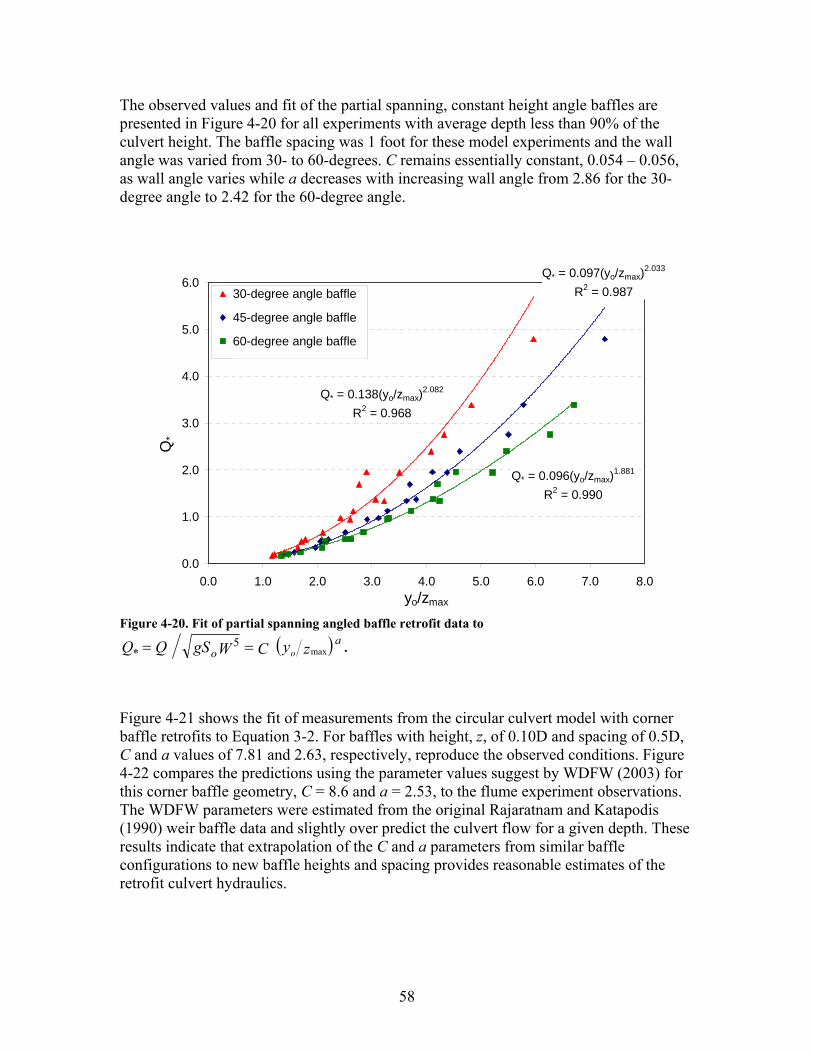
The observed values and fit of the partial spanning, constant height angle baffles are presented in Figure 4-20 for all experiments with average depth less than 90% of the culvert height. The baffle spacing was 1 foot for these model experiments and the wall angle was varied from 30- to 60-degrees. C remains essentially constant, 0.054 – 0.056, as wall angle varies while a decreases with increasing wall angle from 2.86 for the 30-degree angle to 2.42 for the 60-degree angle.

Q* = 0.138(yo/zmax)2.082

R2 = 0.968

Q* = 0.097(yo/zmax)2.033

R2 = 0.987

Q* = 0.096(yo/zmax)1.881

R2 = 0.990

0.0

1.0

2.0

3.0

4.0

5.0

6.0

0.0 1.0 2.0 3.0 4.0 5.0 6.0 7.0 8.0yo/zmax

Q*

30-degree angle baffle

45-degree angle baffle

60-degree angle baffle

Figure 4-20. Fit of partial spanning angled baffle retrofit data to

( )zyCWgSQQ oa

o max 5

* == .

Figure 4-21 shows the fit of measurements from the circular culvert model with corner baffle retrofits to Equation 3-2. For baffles with height, z, of 0.10D and spacing of 0.5D, C and a values of 7.81 and 2.63, respectively, reproduce the observed conditions. Figure 4-22 compares the predictions using the parameter values suggest by WDFW (2003) for this corner baffle geometry, C = 8.6 and a = 2.53, to the flume experiment observations. The WDFW parameters were estimated from the original Rajaratnam and Katapodis (1990) weir baffle data and slightly over predict the culvert flow for a given depth. These results indicate that extrapolation of the C and a parameters from similar baffle configurations to new baffle heights and spacing provides reasonable estimates of the retrofit culvert hydraulics.

58

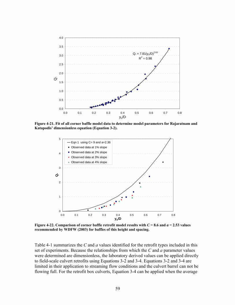
Q* = 7.81(yo/D)2.63

R2 = 0.98

0.0

0.5

1.0

1.5

2.0

2.5

3.0

3.5

4.0

0.0 0.1 0.2 0.3 0.4 0.5 0.6 0.7 0.8yo/D

Q*

Figure 4-21. Fit of all corner baffle model data to determine model parameters for Rajaratnam and Katapodis’ dimensionless equation (Equation 3-2).

0

1

2

3

4

5

0.0 0.1 0.2 0.3 0.4 0.5 0.6 0.7 0.8yo/D

Q*

Eqn 1 using C= 9 and a=2.36Observed data at 1% slopeObserved data at 2% slopeObserved data at 3% slopeObserved data at 4% slope

Figure 4-22. Comparison of corner baffle retrofit model results with C = 8.6 and a = 2.53 values recommended by WDFW (2003) for baffles of this height and spacing. Table 4-1 summarizes the C and a values identified for the retrofit types included in this set of experiments. Because the relationships from which the C and a parameter values were determined are dimensionless, the laboratory derived values can be applied directly to field-scale culvert retrofits using Equations 3-2 and 3-4. Equations 3-2 and 3-4 are limited in their application to streaming flow conditions and the culvert barrel can not be flowing full. For the retrofit box culverts, Equation 3-4 can be applied when the average

59

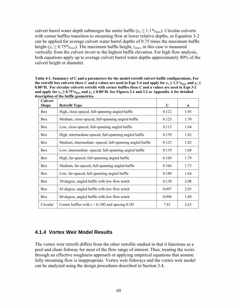
culvert barrel water depth submerges the entire baffle (yo ≥ 1.1*zmax). Circular culverts with corner baffles transition to streaming flow at lower relative depths, so Equation 3-2 can be applied for average culvert water barrel depths of 0.75 times the maximum baffle height (yo ≥ 0.75*zmax). The maximum baffle height, zmax, in this case is measured vertically from the culvert invert to the highest baffle elevation. For high flow analysis, both equations apply up to average culvert barrel water depths approximately 80% of the culvert height or diameter. Table 4-1. Summary of C and a parameters for the model retrofit culvert baffle configurations. For the retrofit box culverts these C and a values are used in Eqn 3-4 and apply for yo ≥ 1.1*zmax and yo ≤ 0.80*H. For circular culverts retrofit with corner baffles these C and a values are used in Eqn 3-2 and apply for yo ≥ 0.75*zmax and yo ≤ 0.80*H. See Figures 3.1 and 3.2 or Appendix A for detailed description of the baffle geometries.

Culvert Shape Retrofit Type C a Box High, close-spaced, full-spanning angled baffle 0.122 1.85

Box Medium, close-spaced, full-spanning angled baffle 0.123 1.70

Box Low, close-spaced, full-spanning angled baffle 0.113 1.64

Box High, intermediate-spaced, full-spanning angled baffle 0.139 1.82

Box Medium, intermediate -spaced, full-spanning angled baffle 0.125 1.82

Box Low, intermediate -spaced, full-spanning angled baffle 0.119 1.68

Box High, far-spaced, full-spanning angled baffle 0.169 1.79

Box Medium, far-spaced, full-spanning angled baffle 0.166 1.73

Box Low, far-spaced, full-spanning angled baffle 0.180 1.64

Box 30-degree, angled baffle with low flow notch 0.138 2.08

Box 45-degree, angled baffle with low flow notch 0.097 2.03

Box 60-degree, angled baffle with low flow notch 0.096 1.88

Circular Corner baffles with z = 0.10D and spacing 0.5D 7.81 2.63

4.1.4 Vortex Weir Model Results The vortex weir retrofit differs from the other retrofits studied in that it functions as a pool and chute fishway for most of the flow range of interest. Thus, treating the weirs through an effective roughness approach or applying empirical equations that assume fully streaming flow is inappropriate. Vortex weir fishways and the vortex weir model can be analyzed using the design procedures described in Section 3.4.

60

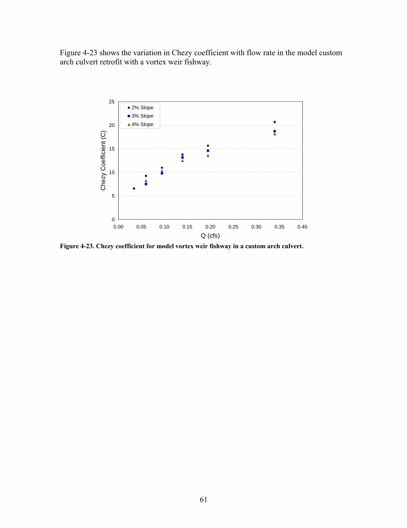
Figure 4-23 shows the variation in Chezy coefficient with flow rate in the model custom arch culvert retrofit with a vortex weir fishway.

0

5

10

15

20

25

0.00 0.05 0.10 0.15 0.20 0.25 0.30 0.35 0.40

Q (cfs)

Che

zy C

oeffi

cien

t (C

)2% Slope3% Slope4% Slope

Figure 4-23. Chezy coefficient for model vortex weir fishway in a custom arch culvert.

61

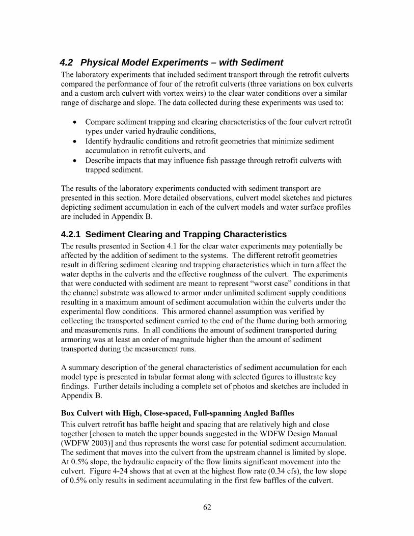
4.2 Physical Model Experiments – with Sediment The laboratory experiments that included sediment transport through the retrofit culverts compared the performance of four of the retrofit culverts (three variations on box culverts and a custom arch culvert with vortex weirs) to the clear water conditions over a similar range of discharge and slope. The data collected during these experiments was used to:

• Compare sediment trapping and clearing characteristics of the four culvert retrofit types under varied hydraulic conditions,

• Identify hydraulic conditions and retrofit geometries that minimize sediment accumulation in retrofit culverts, and

• Describe impacts that may influence fish passage through retrofit culverts with trapped sediment.

The results of the laboratory experiments conducted with sediment transport are presented in this section. More detailed observations, culvert model sketches and pictures depicting sediment accumulation in each of the culvert models and water surface profiles are included in Appendix B.

4.2.1 Sediment Clearing and Trapping Characteristics The results presented in Section 4.1 for the clear water experiments may potentially be affected by the addition of sediment to the systems. The different retrofit geometries result in differing sediment clearing and trapping characteristics which in turn affect the water depths in the culverts and the effective roughness of the culvert. The experiments that were conducted with sediment are meant to represent “worst case” conditions in that the channel substrate was allowed to armor under unlimited sediment supply conditions resulting in a maximum amount of sediment accumulation within the culverts under the experimental flow conditions. This armored channel assumption was verified by collecting the transported sediment carried to the end of the flume during both armoring and measurements runs. In all conditions the amount of sediment transported during armoring was at least an order of magnitude higher than the amount of sediment transported during the measurement runs. A summary description of the general characteristics of sediment accumulation for each model type is presented in tabular format along with selected figures to illustrate key findings. Further details including a complete set of photos and sketches are included in Appendix B.

Box Culvert with High, Close-spaced, Full-spanning Angled Baffles This culvert retrofit has baffle height and spacing that are relatively high and close together [chosen to match the upper bounds suggested in the WDFW Design Manual (WDFW 2003)] and thus represents the worst case for potential sediment accumulation. The sediment that moves into the culvert from the upstream channel is limited by slope. At 0.5% slope, the hydraulic capacity of the flow limits significant movement into the culvert. Figure 4-24 shows that at even at the highest flow rate (0.34 cfs), the low slope of 0.5% only results in sediment accumulating in the first few baffles of the culvert.

62

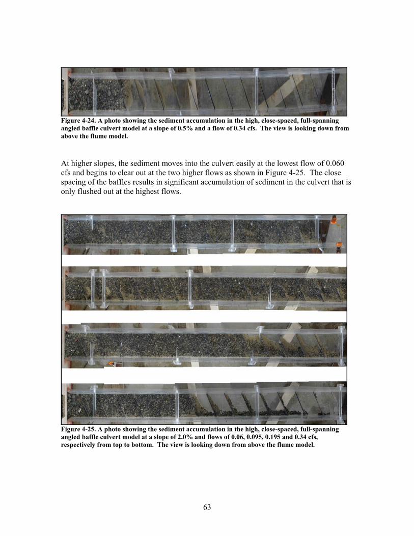
Figure 4-24. A photo showing the sediment accumulation in the high, close-spaced, full-spanning angled baffle culvert model at a slope of 0.5% and a flow of 0.34 cfs. The view is looking down from above the flume model. At higher slopes, the sediment moves into the culvert easily at the lowest flow of 0.060 cfs and begins to clear out at the two higher flows as shown in Figure 4-25. The close spacing of the baffles results in significant accumulation of sediment in the culvert that is only flushed out at the highest flows.

Figure 4-25. A photo showing the sediment accumulation in the high, close-spaced, full-spanning angled baffle culvert model at a slope of 2.0% and flows of 0.06, 0.095, 0.195 and 0.34 cfs, respectively from top to bottom. The view is looking down from above the flume model.

63

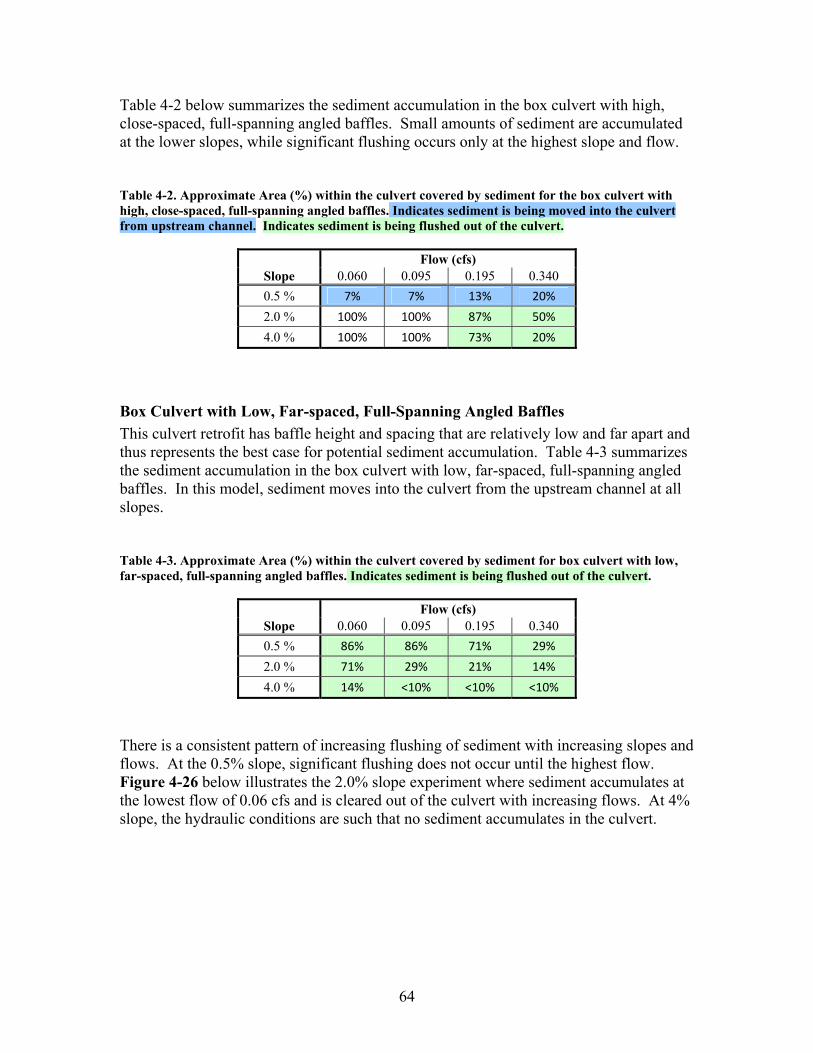
Table 4-2 below summarizes the sediment accumulation in the box culvert with high, close-spaced, full-spanning angled baffles. Small amounts of sediment are accumulated at the lower slopes, while significant flushing occurs only at the highest slope and flow. Table 4-2. Approximate Area (%) within the culvert covered by sediment for the box culvert with high, close-spaced, full-spanning angled baffles. Indicates sediment is being moved into the culvert from upstream channel. Indicates sediment is being flushed out of the culvert.

Flow (cfs)

Slope 0.060 0.095 0.195 0.340 0.5 % 7%  7%  13%  20% 

2.0 % 100%  100%  87%  50% 

4.0 % 100%  100%  73%  20% 

Box Culvert with Low, Far-spaced, Full-Spanning Angled Baffles This culvert retrofit has baffle height and spacing that are relatively low and far apart and thus represents the best case for potential sediment accumulation. Table 4-3 summarizes the sediment accumulation in the box culvert with low, far-spaced, full-spanning angled baffles. In this model, sediment moves into the culvert from the upstream channel at all slopes. Table 4-3. Approximate Area (%) within the culvert covered by sediment for box culvert with low, far-spaced, full-spanning angled baffles. Indicates sediment is being flushed out of the culvert.

Flow (cfs)

Slope 0.060 0.095 0.195 0.340 0.5 % 86%  86%  71%  29% 

2.0 % 71%  29%  21%  14% 

4.0 % 14%  <10%  <10%  <10% 

There is a consistent pattern of increasing flushing of sediment with increasing slopes and flows. At the 0.5% slope, significant flushing does not occur until the highest flow. Figure 4-26 below illustrates the 2.0% slope experiment where sediment accumulates at the lowest flow of 0.06 cfs and is cleared out of the culvert with increasing flows. At 4% slope, the hydraulic conditions are such that no sediment accumulates in the culvert.

64

Figure 4-26. A photo showing the sediment accumulation in the low, far-spaced, full-spanning angled baffle culvert model at a slope of 2.0% and flows of 0.06, 0.095, 0.195 and 0.34 cfs, respectively, from top to bottom. The view is looking down from above the flume model. Box Culvert with 30º Wall Angle, Partial-spanning Baffles Table 4-4 summarizes the sediment accumulation in the box culvert retrofit with 30º wall angle, partial-spanning baffles. As indicated by the shading the hydraulic capacity to bring sediment into the culvert from the upstream channel is not sufficient at the 0.5% slope. At the 2% and 4% slopes, there is a consistent pattern of increasing flushing of sediment with increasing slopes and flows. The culvert is significantly scoured clean only at the highest slope of 4%. Table 4-4. Approximate Area (%) within the culvert covered by sediment for the 30º wall angle, partial-spanning baffles. Indicates sediment is being moved into the culvert from upstream channel. Indicates sediment is being flushed out of the culvert.

Flow (cfs)

Slope 0.060 0.095 0.195 0.340 0.5 % 29%  29%  21%  21%

2.0 % 86%  57%  29%  29%

4.0 % 43%  36%  29%  14%

Custom Arch Culvert with Vortex Weirs The custom arch culvert model with vortex weirs was scaled from the design for the Luffenholtz Creek culvert retrofit implemented by Caltrans. This model was the largest culvert model and flume flow rates that significantly submerged the culvert inlet were not

65

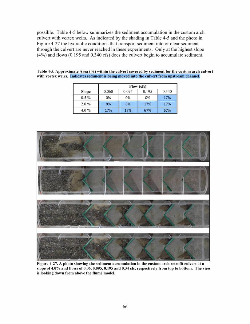
possible. Table 4-5 below summarizes the sediment accumulation in the custom arch culvert with vortex weirs. As indicated by the shading in Table 4-5 and the photo in Figure 4-27 the hydraulic conditions that transport sediment into or clear sediment through the culvert are never reached in these experiments. Only at the highest slope (4%) and flows (0.195 and 0.340 cfs) does the culvert begin to accumulate sediment. Table 4-5. Approximate Area (%) within the culvert covered by sediment for the custom arch culvert with vortex weirs. Indicates sediment is being moved into the culvert from upstream channel.

Flow (cfs)

Slope 0.060 0.095 0.195 0.340 0.5 % 0%  0%  0%  17% 

2.0 % 8%  8%  17%  17% 

4.0 % 17%  17%  67%  67% 

Figure 4-27. A photo showing the sediment accumulation in the custom arch retrofit culvert at a slope of 4.0% and flows of 0.06, 0.095, 0.195 and 0.34 cfs, respectively from top to bottom. The view is looking down from above the flume model.

66

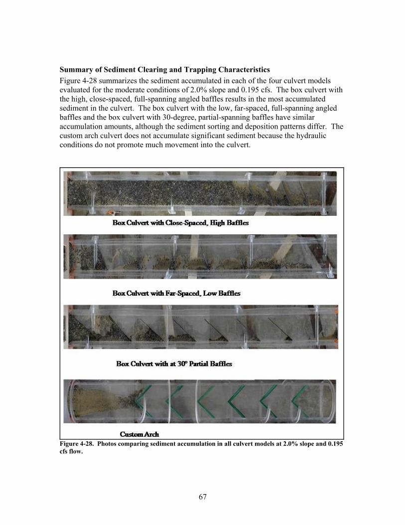
Summary of Sediment Clearing and Trapping Characteristics Figure 4-28 summarizes the sediment accumulated in each of the four culvert models evaluated for the moderate conditions of 2.0% slope and 0.195 cfs. The box culvert with the high, close-spaced, full-spanning angled baffles results in the most accumulated sediment in the culvert. The box culvert with the low, far-spaced, full-spanning angled baffles and the box culvert with 30-degree, partial-spanning baffles have similar accumulation amounts, although the sediment sorting and deposition patterns differ. The custom arch culvert does not accumulate significant sediment because the hydraulic conditions do not promote much movement into the culvert.

Figure 4-28. Photos comparing sediment accumulation in all culvert models at 2.0% slope and 0.195 cfs flow.

67

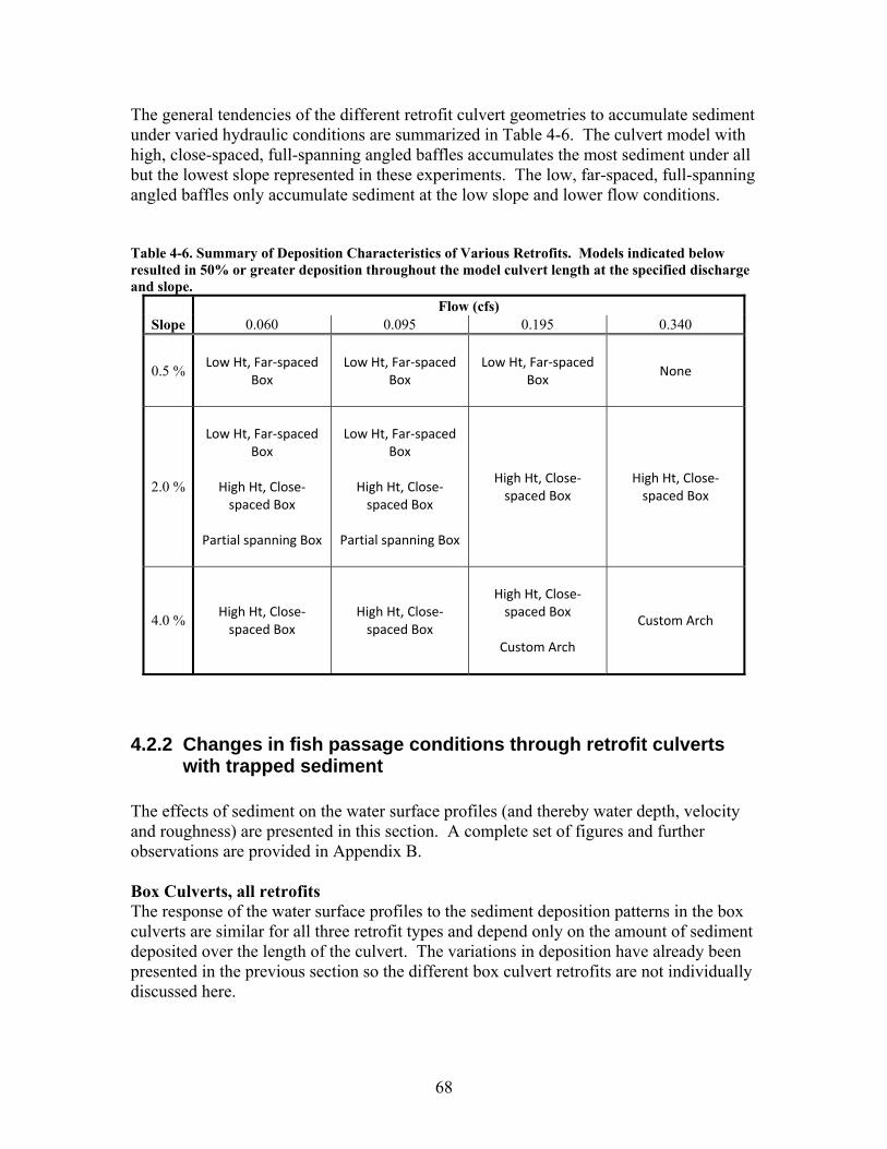
The general tendencies of the different retrofit culvert geometries to accumulate sediment under varied hydraulic conditions are summarized in Table 4-6. The culvert model with high, close-spaced, full-spanning angled baffles accumulates the most sediment under all but the lowest slope represented in these experiments. The low, far-spaced, full-spanning angled baffles only accumulate sediment at the low slope and lower flow conditions. Table 4-6. Summary of Deposition Characteristics of Various Retrofits. Models indicated below resulted in 50% or greater deposition throughout the model culvert length at the specified discharge and slope.

Flow (cfs) Slope 0.060 0.095 0.195 0.340

0.5 %

 Low Ht, Far‐spaced 

Box  

Low Ht, Far‐spaced Box 

Low Ht, Far‐spaced Box 

None 

2.0 %

 Low Ht, Far‐spaced 

Box  

High Ht, Close‐spaced Box 

 Partial spanning Box 

 

Low Ht, Far‐spaced Box  

High Ht, Close‐spaced Box 

 Partial spanning Box 

High Ht, Close‐spaced Box 

High Ht, Close‐spaced Box 

4.0 % High Ht, Close‐spaced Box 

High Ht, Close‐spaced Box 

 High Ht, Close‐spaced Box  

 Custom Arch 

 

Custom Arch 

4.2.2 Changes in fish passage conditions through retrofit culverts with trapped sediment

The effects of sediment on the water surface profiles (and thereby water depth, velocity and roughness) are presented in this section. A complete set of figures and further observations are provided in Appendix B. Box Culverts, all retrofits The response of the water surface profiles to the sediment deposition patterns in the box culverts are similar for all three retrofit types and depend only on the amount of sediment deposited over the length of the culvert. The variations in deposition have already been presented in the previous section so the different box culvert retrofits are not individually discussed here.

68

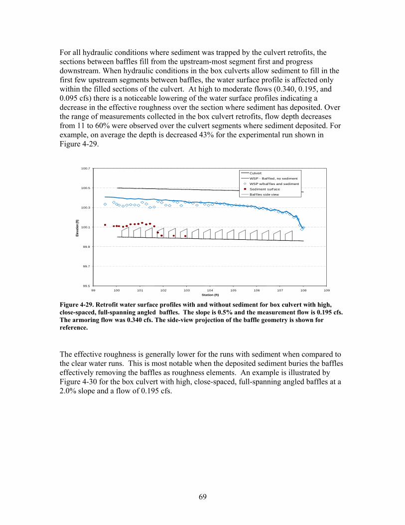
For all hydraulic conditions where sediment was trapped by the culvert retrofits, the sections between baffles fill from the upstream-most segment first and progress downstream. When hydraulic conditions in the box culverts allow sediment to fill in the first few upstream segments between baffles, the water surface profile is affected only within the filled sections of the culvert. At high to moderate flows (0.340, 0.195, and 0.095 cfs) there is a noticeable lowering of the water surface profiles indicating a decrease in the effective roughness over the section where sediment has deposited. Over the range of measurements collected in the box culvert retrofits, flow depth decreases from 11 to 60% were observed over the culvert segments where sediment deposited. For example, on average the depth is decreased 43% for the experimental run shown in Figure 4-29.

99.5

99.7

99.9

100.1

100.3

100.5

100.7

99 100 101 102 103 104 105 106 107 108 109

Elev

ation

(ft)

Station (ft)

Culvert

WSP - Baf f led, no sediment

WSP w/baf f les and sediment

Sediment surface

Baf f les side view

Figure 4-29. Retrofit water surface profiles with and without sediment for box culvert with high, close-spaced, full-spanning angled baffles. The slope is 0.5% and the measurement flow is 0.195 cfs. The armoring flow was 0.340 cfs. The side-view projection of the baffle geometry is shown for reference. The effective roughness is generally lower for the runs with sediment when compared to the clear water runs. This is most notable when the deposited sediment buries the baffles effectively removing the baffles as roughness elements. An example is illustrated by Figure 4-30 for the box culvert with high, close-spaced, full-spanning angled baffles at a 2.0% slope and a flow of 0.195 cfs.

69

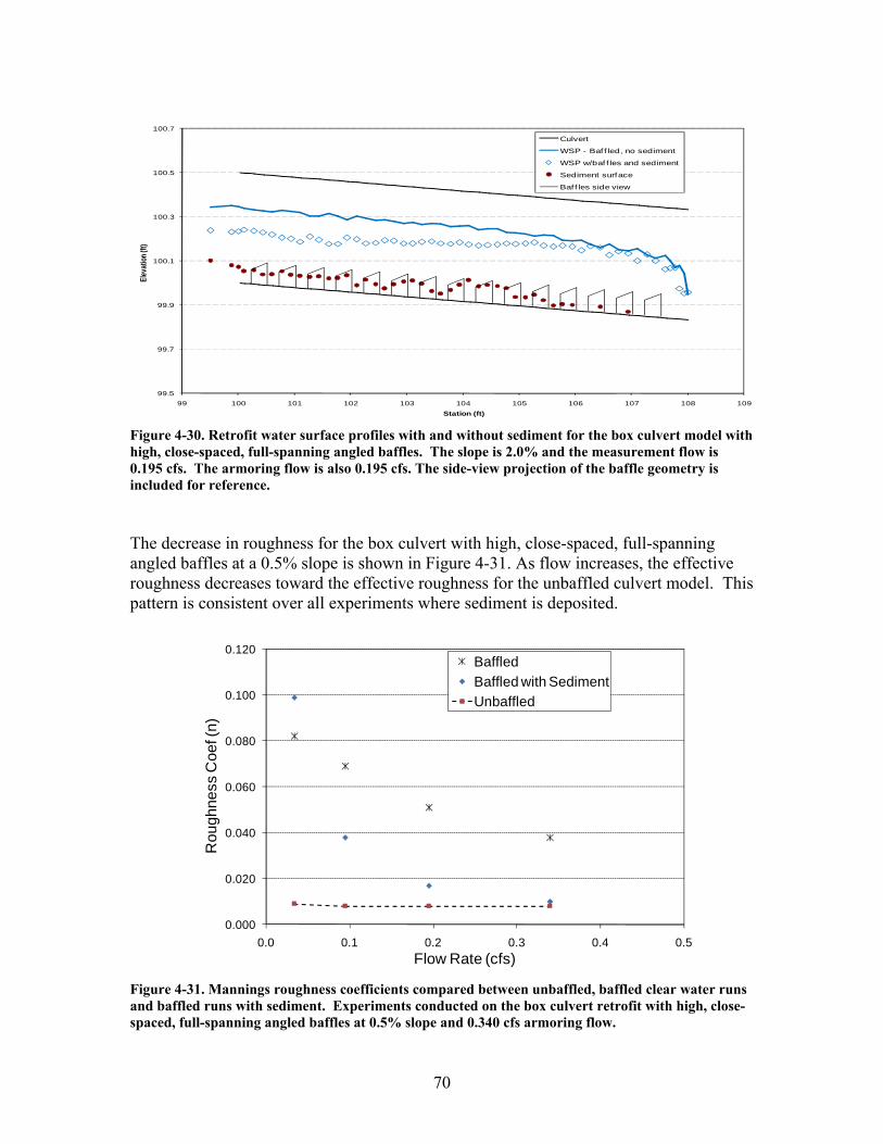
99.5

99.7

99.9

100.1

100.3

100.5

100.7

99 100 101 102 103 104 105 106 107 108 109

Eleva

tion (

ft)

Station (ft)

Culvert

WSP - Baff led, no sediment

WSP w/baf f les and sediment

Sediment surface

Baff les side view

Figure 4-30. Retrofit water surface profiles with and without sediment for the box culvert model with high, close-spaced, full-spanning angled baffles. The slope is 2.0% and the measurement flow is 0.195 cfs. The armoring flow is also 0.195 cfs. The side-view projection of the baffle geometry is included for reference. The decrease in roughness for the box culvert with high, close-spaced, full-spanning angled baffles at a 0.5% slope is shown in Figure 4-31. As flow increases, the effective roughness decreases toward the effective roughness for the unbaffled culvert model. This pattern is consistent over all experiments where sediment is deposited.

0.000

0.020

0.040

0.060

0.080

0.100

0.120

0.0 0.1 0.2 0.3 0.4 0.5

Rou

ghne

ss C

oef (

n)

Flow Rate (cfs)

Baffled Baffled with SedimentUnbaffled

Figure 4-31. Mannings roughness coefficients compared between unbaffled, baffled clear water runs and baffled runs with sediment. Experiments conducted on the box culvert retrofit with high, close-spaced, full-spanning angled baffles at 0.5% slope and 0.340 cfs armoring flow.

70

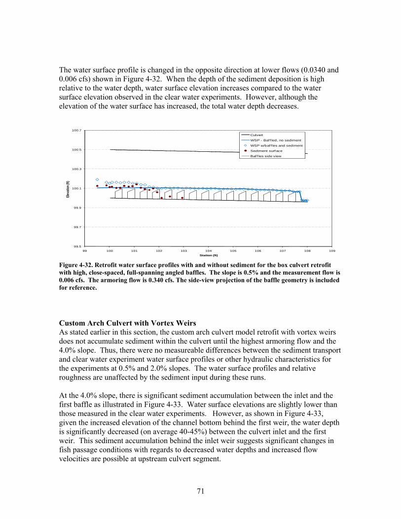
The water surface profile is changed in the opposite direction at lower flows (0.0340 and 0.006 cfs) shown in Figure 4-32. When the depth of the sediment deposition is high relative to the water depth, water surface elevation increases compared to the water surface elevation observed in the clear water experiments. However, although the elevation of the water surface has increased, the total water depth decreases.

99.5

99.7

99.9

100.1

100.3

100.5

100.7

99 100 101 102 103 104 105 106 107 108 109

Eleva

tion (

ft)

Station (ft)

Culvert

WSP - Baf f led, no sediment

WSP w/baf f les and sediment

Sediment surface

Baf f les side view

Figure 4-32. Retrofit water surface profiles with and without sediment for the box culvert retrofit with high, close-spaced, full-spanning angled baffles. The slope is 0.5% and the measurement flow is 0.006 cfs. The armoring flow is 0.340 cfs. The side-view projection of the baffle geometry is included for reference. Custom Arch Culvert with Vortex Weirs As stated earlier in this section, the custom arch culvert model retrofit with vortex weirs does not accumulate sediment within the culvert until the highest armoring flow and the 4.0% slope. Thus, there were no measureable differences between the sediment transport and clear water experiment water surface profiles or other hydraulic characteristics for the experiments at 0.5% and 2.0% slopes. The water surface profiles and relative roughness are unaffected by the sediment input during these runs. At the 4.0% slope, there is significant sediment accumulation between the inlet and the first baffle as illustrated in Figure 4-33. Water surface elevations are slightly lower than those measured in the clear water experiments. However, as shown in Figure 4-33, given the increased elevation of the channel bottom behind the first weir, the water depth is significantly decreased (on average 40-45%) between the culvert inlet and the first weir. This sediment accumulation behind the inlet weir suggests significant changes in fish passage conditions with regards to decreased water depths and increased flow velocities are possible at upstream culvert segment.

71

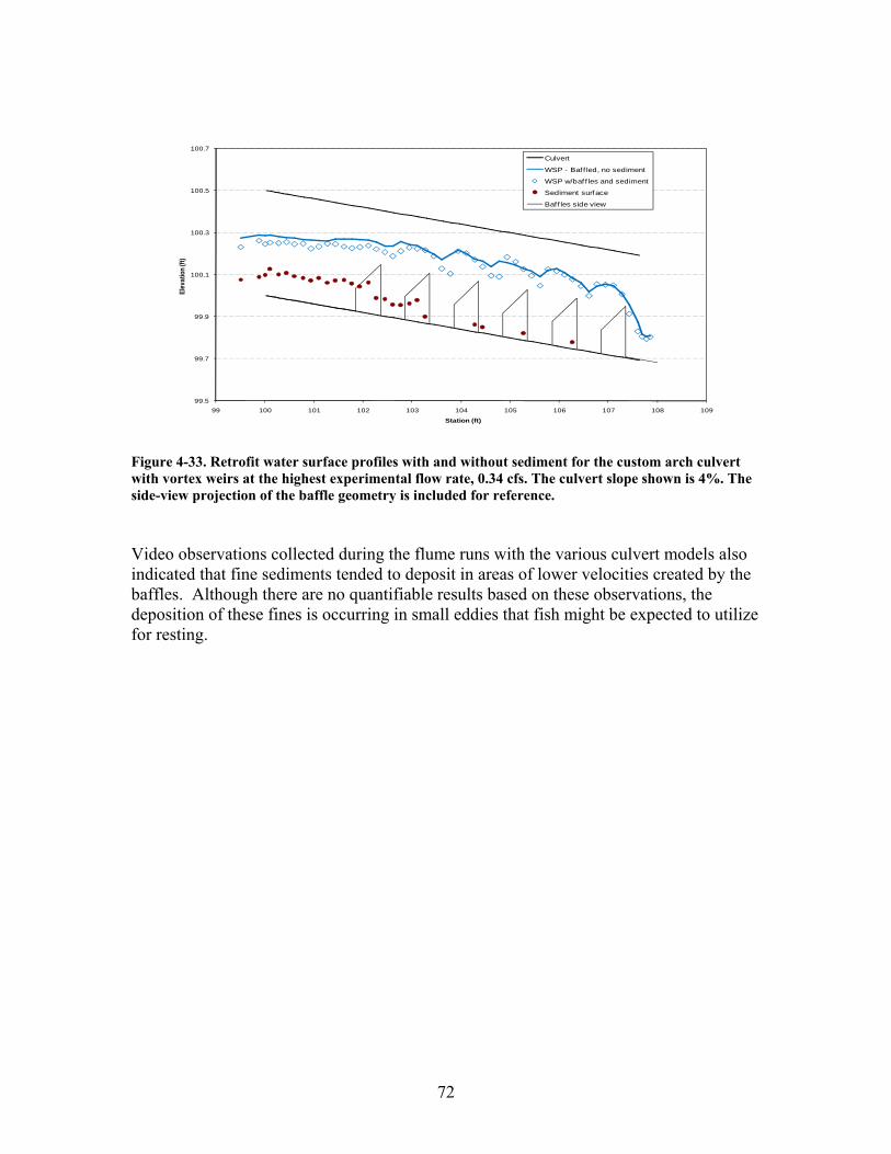
99.5

99.7

99.9

100.1

100.3

100.5

100.7

99 100 101 102 103 104 105 106 107 108 109

Elev

ation

(ft)

Station (ft)

Culvert

WSP - Baf f led, no sediment

WSP w/baf f les and sediment

Sediment surface

Baff les side view

Figure 4-33. Retrofit water surface profiles with and without sediment for the custom arch culvert with vortex weirs at the highest experimental flow rate, 0.34 cfs. The culvert slope shown is 4%. The side-view projection of the baffle geometry is included for reference. Video observations collected during the flume runs with the various culvert models also indicated that fine sediments tended to deposit in areas of lower velocities created by the baffles. Although there are no quantifiable results based on these observations, the deposition of these fines is occurring in small eddies that fish might be expected to utilize for resting.

72

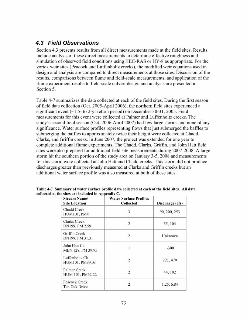
4.3 Field Observations Section 4.3 presents results from all direct measurements made at the field sites. Results include analysis of these direct measurements to determine effective roughness and simulation of observed field conditions using HEC-RAS or HY-8 as appropriate. For the vortex weir sites (Peacock and Luffenholtz creeks), the modified weir equations used in design and analysis are compared to direct measurements at those sites. Discussion of the results, comparisons between flume and field-scale measurements, and application of the flume experiment results to field-scale culvert design and analysis are presented in Section 5. Table 4-7 summarizes the data collected at each of the field sites. During the first season of field data collection (Oct. 2005-April 2006), the northern field sites experienced a significant event (~1.5- to 2-yr return period) on December 30-31, 2005. Field measurements for this event were collected at Palmer and Luffenholtz creeks. The study’s second field season (Oct. 2006-April 2007) had few large storms and none of any significance. Water surface profiles representing flows that just submerged the baffles to submerging the baffles to approximately twice their height were collected at Chadd, Clarks, and Griffin creeks. In June 2007, the project was extended for one year to complete additional flume experiments. The Chadd, Clarks, Griffin, and John Hatt field sites were also prepared for additional field site measurements during 2007-2008. A large storm hit the southern portion of the study area on January 3-5, 2008 and measurements for this storm were collected at John Hatt and Chadd creeks. This storm did not produce discharges greater than previously measured at Clarks and Griffin creeks but an additional water surface profile was also measured at both of these sites. Table 4-7. Summary of water surface profile data collected at each of the field sites. All data collected at the sites are included in Appendix C.

Stream Name/ Site Location

Water Surface Profiles Collected Discharge (cfs)

Chadd Creek HUM101, PM4 3 90, 200, 253

Clarks Creek DN199, PM 2.59 2 55, 104

Griffin Creek DN199, PM 31.31 2 Unknown

John Hatt Ck MEN 128, PM 39.95 1 ~300

Luffenholtz Ck HUM101, PM99.03 2 221, 470

Palmer Creek HUM 101, PM62.22 2 44, 102

Peacock Creek Tan Oak Drive 2 1.25, 6.84

73

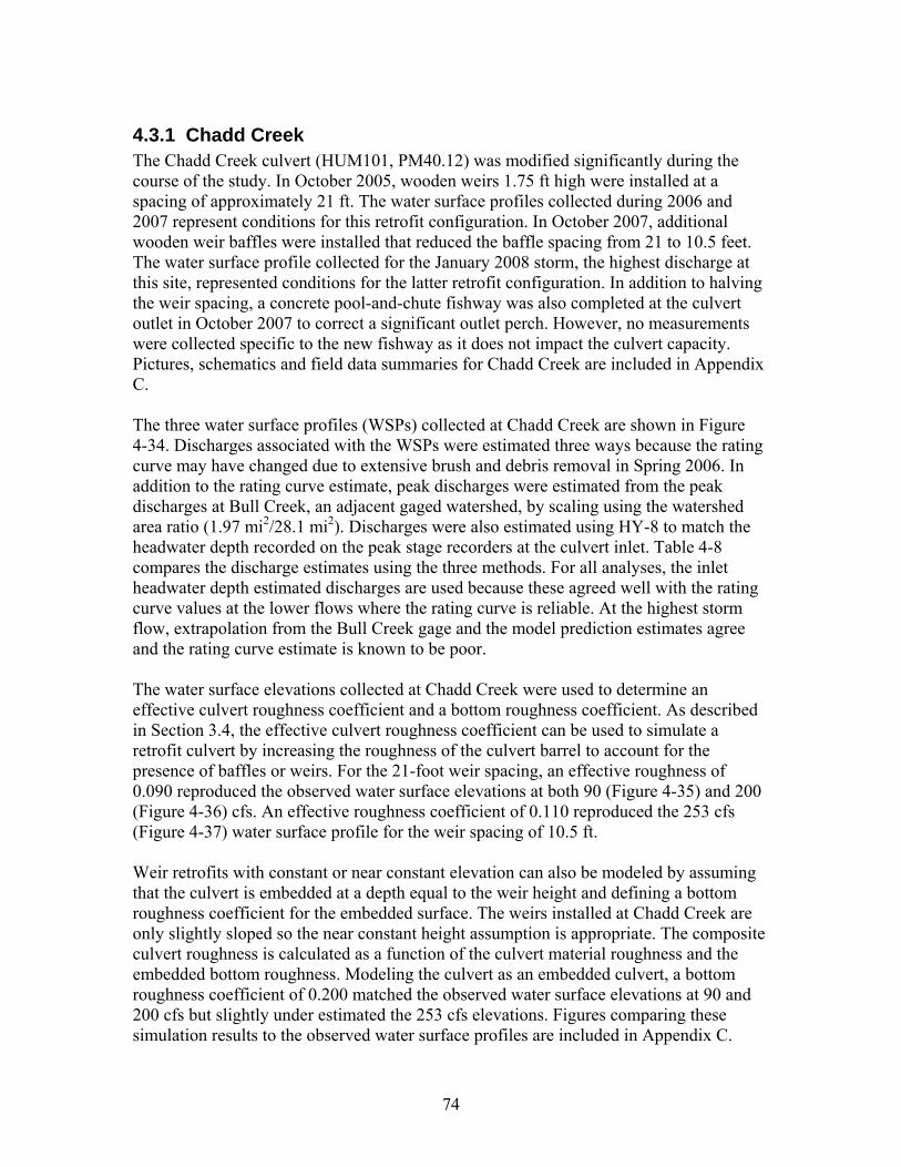
4.3.1 Chadd Creek The Chadd Creek culvert (HUM101, PM40.12) was modified significantly during the course of the study. In October 2005, wooden weirs 1.75 ft high were installed at a spacing of approximately 21 ft. The water surface profiles collected during 2006 and 2007 represent conditions for this retrofit configuration. In October 2007, additional wooden weir baffles were installed that reduced the baffle spacing from 21 to 10.5 feet. The water surface profile collected for the January 2008 storm, the highest discharge at this site, represented conditions for the latter retrofit configuration. In addition to halving the weir spacing, a concrete pool-and-chute fishway was also completed at the culvert outlet in October 2007 to correct a significant outlet perch. However, no measurements were collected specific to the new fishway as it does not impact the culvert capacity. Pictures, schematics and field data summaries for Chadd Creek are included in Appendix C. The three water surface profiles (WSPs) collected at Chadd Creek are shown in Figure 4-34. Discharges associated with the WSPs were estimated three ways because the rating curve may have changed due to extensive brush and debris removal in Spring 2006. In addition to the rating curve estimate, peak discharges were estimated from the peak discharges at Bull Creek, an adjacent gaged watershed, by scaling using the watershed area ratio (1.97 mi2/28.1 mi2). Discharges were also estimated using HY-8 to match the headwater depth recorded on the peak stage recorders at the culvert inlet. Table 4-8 compares the discharge estimates using the three methods. For all analyses, the inlet headwater depth estimated discharges are used because these agreed well with the rating curve values at the lower flows where the rating curve is reliable. At the highest storm flow, extrapolation from the Bull Creek gage and the model prediction estimates agree and the rating curve estimate is known to be poor. The water surface elevations collected at Chadd Creek were used to determine an effective culvert roughness coefficient and a bottom roughness coefficient. As described in Section 3.4, the effective culvert roughness coefficient can be used to simulate a retrofit culvert by increasing the roughness of the culvert barrel to account for the presence of baffles or weirs. For the 21-foot weir spacing, an effective roughness of 0.090 reproduced the observed water surface elevations at both 90 (Figure 4-35) and 200 (Figure 4-36) cfs. An effective roughness coefficient of 0.110 reproduced the 253 cfs (Figure 4-37) water surface profile for the weir spacing of 10.5 ft. Weir retrofits with constant or near constant elevation can also be modeled by assuming that the culvert is embedded at a depth equal to the weir height and defining a bottom roughness coefficient for the embedded surface. The weirs installed at Chadd Creek are only slightly sloped so the near constant height assumption is appropriate. The composite culvert roughness is calculated as a function of the culvert material roughness and the embedded bottom roughness. Modeling the culvert as an embedded culvert, a bottom roughness coefficient of 0.200 matched the observed water surface elevations at 90 and 200 cfs but slightly under estimated the 253 cfs elevations. Figures comparing these simulation results to the observed water surface profiles are included in Appendix C.

74

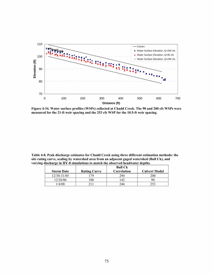
70

80

90

100

110

0 100 200 300 400 500 600 700Distance (ft)

Elev

atio

n (ft

)

Culvert

Water Surface Elevation, Q=200 cfs

Water Surface Elevation, Q=90 cfs

Water Surface Elevation, Q=255 cfs

Figure 4-34. Water surface profiles (WSPs) collected at Chadd Creek. The 90 and 200 cfs WSPs were measured for the 21-ft weir spacing and the 253 cfs WSP for the 10.5-ft weir spacing. Table 4-8. Peak discharge estimates for Chadd Creek using three different estimation methods: the site rating curve, scaling by watershed area from an adjacent gaged watershed (Bull Ck), and varying discharge in HY-8 simulations to match the observed headwater depths.

Storm Date Rating Curve Bull Ck

Correlation Culvert Model 12/30-31/05 179 294 200

12/26/06 100 142 90 1/4/08 211 246 253

75

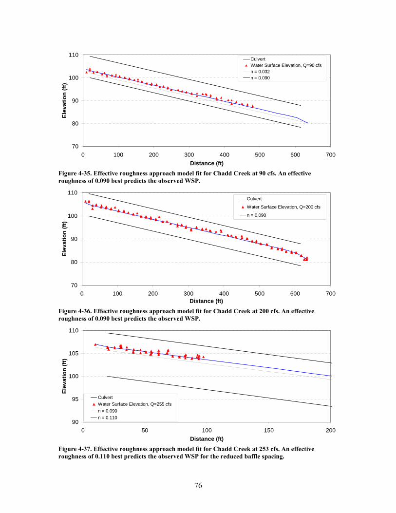
70

80

90

100

110

0 100 200 300 400 500 600 700Distance (ft)

Elev

atio

n (ft

)CulvertWater Surface Elevation, Q=90 cfsn = 0.032n = 0.090

Figure 4-35. Effective roughness approach model fit for Chadd Creek at 90 cfs. An effective roughness of 0.090 best predicts the observed WSP.

70

80

90

100

110

0 100 200 300 400 500 600 700Distance (ft)

Elev

atio

n (ft

)

Culvert

Water Surface Elevation, Q=200 cfs

n = 0.090

Figure 4-36. Effective roughness approach model fit for Chadd Creek at 200 cfs. An effective roughness of 0.090 best predicts the observed WSP.

90

95

100

105

110

0 50 100 150 200Distance (ft)

Elev

atio

n (ft

)

CulvertWater Surface Elevation, Q=255 cfsn = 0.090n = 0.110

Figure 4-37. Effective roughness approach model fit for Chadd Creek at 253 cfs. An effective roughness of 0.110 best predicts the observed WSP for the reduced baffle spacing.

76

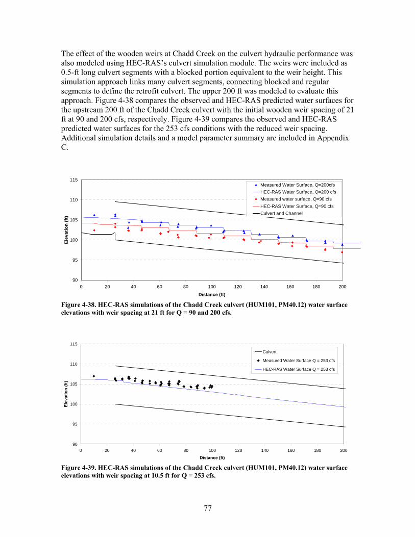
The effect of the wooden weirs at Chadd Creek on the culvert hydraulic performance was also modeled using HEC-RAS’s culvert simulation module. The weirs were included as 0.5-ft long culvert segments with a blocked portion equivalent to the weir height. This simulation approach links many culvert segments, connecting blocked and regular segments to define the retrofit culvert. The upper 200 ft was modeled to evaluate this approach. Figure 4-38 compares the observed and HEC-RAS predicted water surfaces for the upstream 200 ft of the Chadd Creek culvert with the initial wooden weir spacing of 21 ft at 90 and 200 cfs, respectively. Figure 4-39 compares the observed and HEC-RAS predicted water surfaces for the 253 cfs conditions with the reduced weir spacing. Additional simulation details and a model parameter summary are included in Appendix C.

90

95

100

105

110

115

0 20 40 60 80 100 120 140 160 180 200

Distance (ft)

Elev

atio

n (ft

)

Measured Water Surface, Q=200cfsHEC-RAS Water Surface, Q=200 cfsMeasured water surface, Q=90 cfsHEC-RAS Water Surface, Q=90 cfsCulvert and Channel

Figure 4-38. HEC-RAS simulations of the Chadd Creek culvert (HUM101, PM40.12) water surface elevations with weir spacing at 21 ft for Q = 90 and 200 cfs.

90

95

100

105

110

115

0 20 40 60 80 100 120 140 160 180 200

Distance (ft)

Elev

atio

n (ft

)

Culvert

Measured Water Surface Q = 253 cfs

HEC-RAS Water Surface Q = 253 cfs

Figure 4-39. HEC-RAS simulations of the Chadd Creek culvert (HUM101, PM40.12) water surface elevations with weir spacing at 10.5 ft for Q = 253 cfs.

77

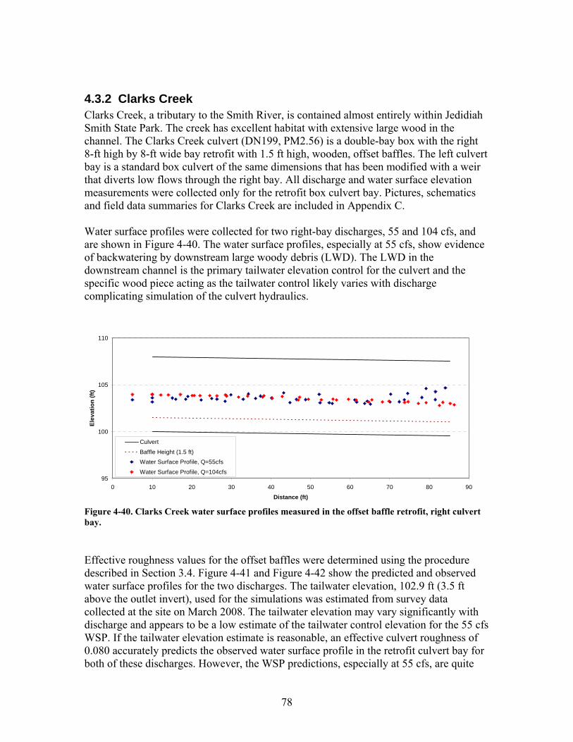
4.3.2 Clarks Creek Clarks Creek, a tributary to the Smith River, is contained almost entirely within Jedidiah Smith State Park. The creek has excellent habitat with extensive large wood in the channel. The Clarks Creek culvert (DN199, PM2.56) is a double-bay box with the right 8-ft high by 8-ft wide bay retrofit with 1.5 ft high, wooden, offset baffles. The left culvert bay is a standard box culvert of the same dimensions that has been modified with a weir that diverts low flows through the right bay. All discharge and water surface elevation measurements were collected only for the retrofit box culvert bay. Pictures, schematics and field data summaries for Clarks Creek are included in Appendix C. Water surface profiles were collected for two right-bay discharges, 55 and 104 cfs, and are shown in Figure 4-40. The water surface profiles, especially at 55 cfs, show evidence of backwatering by downstream large woody debris (LWD). The LWD in the downstream channel is the primary tailwater elevation control for the culvert and the specific wood piece acting as the tailwater control likely varies with discharge complicating simulation of the culvert hydraulics.

95

100

105

110

0 10 20 30 40 50 60 70 80 90

Distance (ft)

Elev

atio

n (ft

)

Culvert

Baffle Height (1.5 ft)Water Surface Profile, Q=55cfs

Water Surface Profile, Q=104cfs

Figure 4-40. Clarks Creek water surface profiles measured in the offset baffle retrofit, right culvert bay. Effective roughness values for the offset baffles were determined using the procedure described in Section 3.4. Figure 4-41 and Figure 4-42 show the predicted and observed water surface profiles for the two discharges. The tailwater elevation, 102.9 ft (3.5 ft above the outlet invert), used for the simulations was estimated from survey data collected at the site on March 2008. The tailwater elevation may vary significantly with discharge and appears to be a low estimate of the tailwater control elevation for the 55 cfs WSP. If the tailwater elevation estimate is reasonable, an effective culvert roughness of 0.080 accurately predicts the observed water surface profile in the retrofit culvert bay for both of these discharges. However, the WSP predictions, especially at 55 cfs, are quite

78

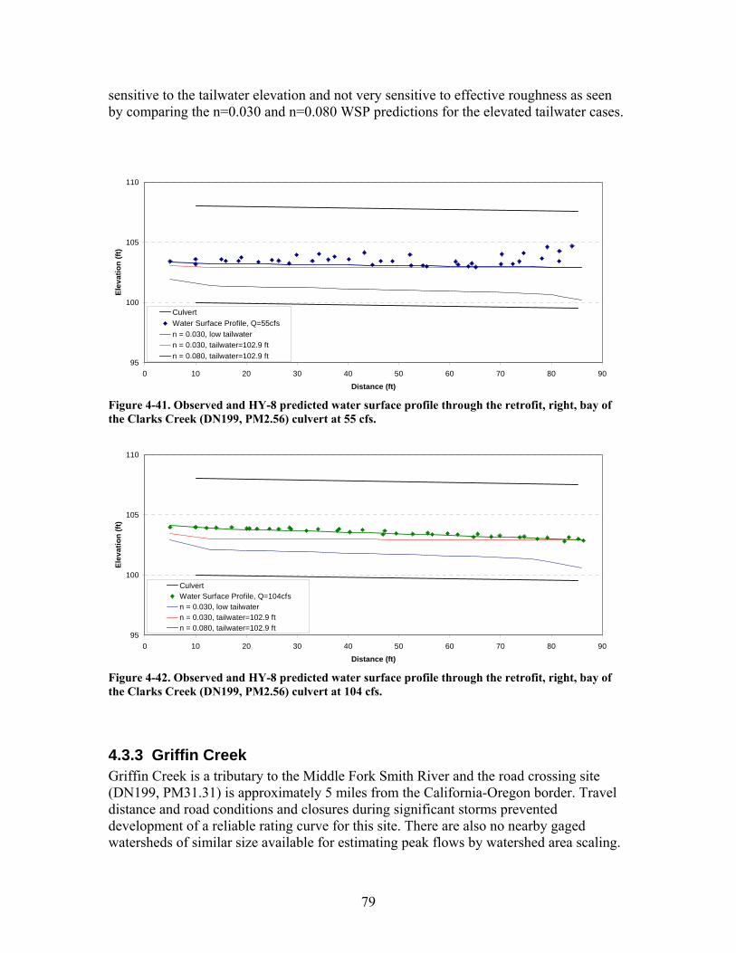
sensitive to the tailwater elevation and not very sensitive to effective roughness as seen by comparing the n=0.030 and n=0.080 WSP predictions for the elevated tailwater cases.

95

100

105

110

0 10 20 30 40 50 60 70 80 90

Distance (ft)

Elev

atio

n (ft

)

CulvertWater Surface Profile, Q=55cfsn = 0.030, low tailwatern = 0.030, tailwater=102.9 ftn = 0.080, tailwater=102.9 ft

Figure 4-41. Observed and HY-8 predicted water surface profile through the retrofit, right, bay of the Clarks Creek (DN199, PM2.56) culvert at 55 cfs.

95

100

105

110

0 10 20 30 40 50 60 70 80 90

Distance (ft)

Elev

atio

n (ft

)

CulvertWater Surface Profile, Q=104cfsn = 0.030, low tailwatern = 0.030, tailwater=102.9 ftn = 0.080, tailwater=102.9 ft

Figure 4-42. Observed and HY-8 predicted water surface profile through the retrofit, right, bay of the Clarks Creek (DN199, PM2.56) culvert at 104 cfs.

4.3.3 Griffin Creek Griffin Creek is a tributary to the Middle Fork Smith River and the road crossing site (DN199, PM31.31) is approximately 5 miles from the California-Oregon border. Travel distance and road conditions and closures during significant storms prevented development of a reliable rating curve for this site. There are also no nearby gaged watersheds of similar size available for estimating peak flows by watershed area scaling.

79

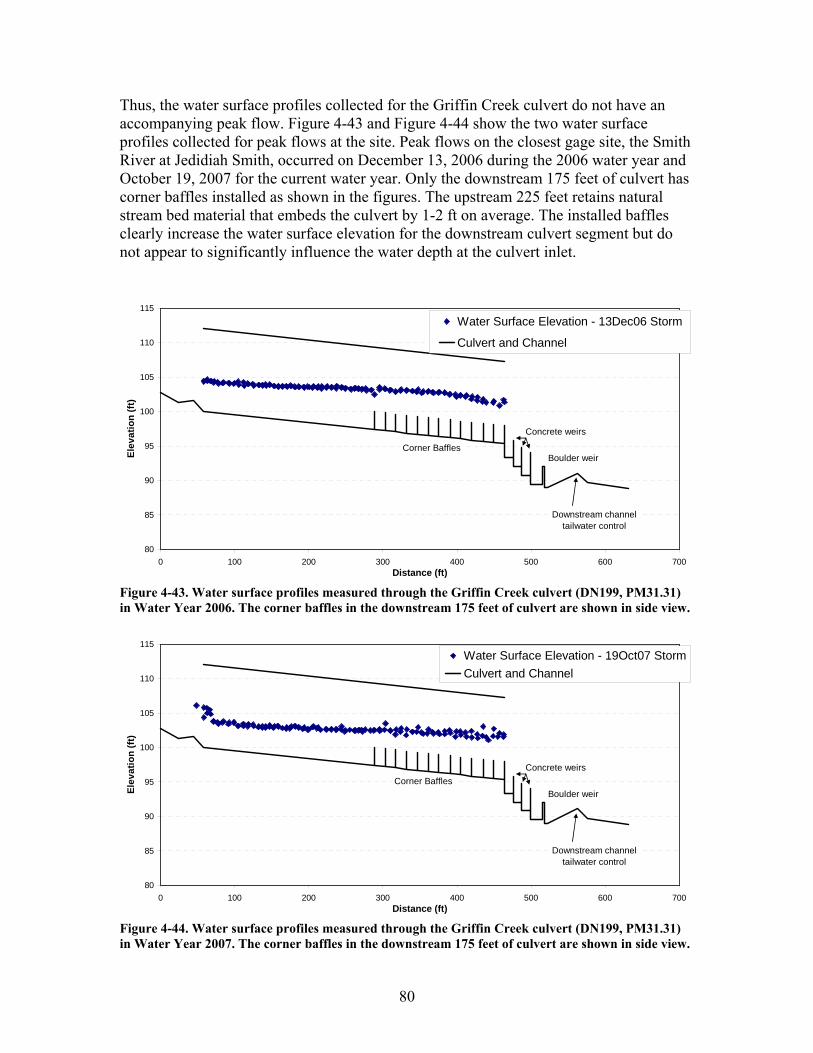
Thus, the water surface profiles collected for the Griffin Creek culvert do not have an accompanying peak flow. Figure 4-43 and Figure 4-44 show the two water surface profiles collected for peak flows at the site. Peak flows on the closest gage site, the Smith River at Jedidiah Smith, occurred on December 13, 2006 during the 2006 water year and October 19, 2007 for the current water year. Only the downstream 175 feet of culvert has corner baffles installed as shown in the figures. The upstream 225 feet retains natural stream bed material that embeds the culvert by 1-2 ft on average. The installed baffles clearly increase the water surface elevation for the downstream culvert segment but do not appear to significantly influence the water depth at the culvert inlet.

80

85

90

95

100

105

110

115

0 100 200 300 400 500 600 700Distance (ft)

Elev

atio

n (ft

)

Water Surface Elevation - 13Dec06 Storm

Culvert and Channel

Concrete weirs

Boulder weir

Downstream channeltailwater control

Corner Baffles

Figure 4-43. Water surface profiles measured through the Griffin Creek culvert (DN199, PM31.31) in Water Year 2006. The corner baffles in the downstream 175 feet of culvert are shown in side view.

80

85

90

95

100

105

110

115

0 100 200 300 400 500 600 700Distance (ft)

Elev

atio

n (ft

)

Water Surface Elevation - 19Oct07 StormCulvert and Channel

Concrete weirs

Boulder weir

Downstream channeltailwater control

Corner Baffles

Figure 4-44. Water surface profiles measured through the Griffin Creek culvert (DN199, PM31.31) in Water Year 2007. The corner baffles in the downstream 175 feet of culvert are shown in side view.

80

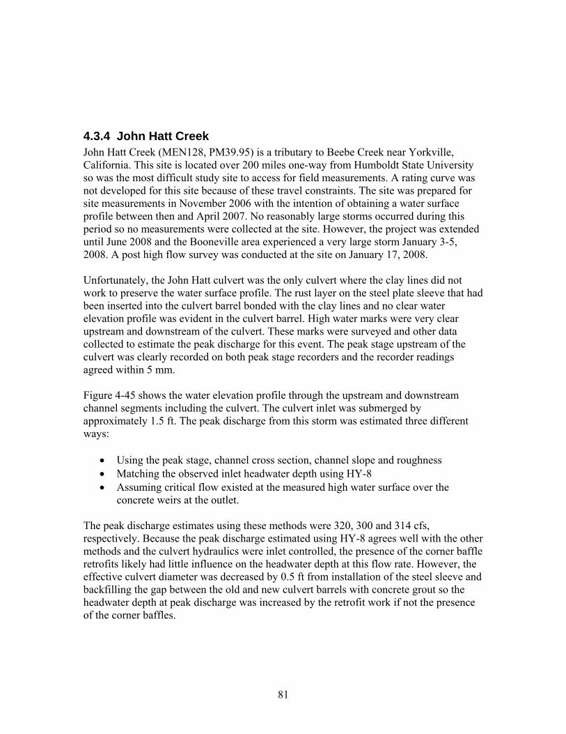
4.3.4 John Hatt Creek John Hatt Creek (MEN128, PM39.95) is a tributary to Beebe Creek near Yorkville, California. This site is located over 200 miles one-way from Humboldt State University so was the most difficult study site to access for field measurements. A rating curve was not developed for this site because of these travel constraints. The site was prepared for site measurements in November 2006 with the intention of obtaining a water surface profile between then and April 2007. No reasonably large storms occurred during this period so no measurements were collected at the site. However, the project was extended until June 2008 and the Booneville area experienced a very large storm January 3-5, 2008. A post high flow survey was conducted at the site on January 17, 2008. Unfortunately, the John Hatt culvert was the only culvert where the clay lines did not work to preserve the water surface profile. The rust layer on the steel plate sleeve that had been inserted into the culvert barrel bonded with the clay lines and no clear water elevation profile was evident in the culvert barrel. High water marks were very clear upstream and downstream of the culvert. These marks were surveyed and other data collected to estimate the peak discharge for this event. The peak stage upstream of the culvert was clearly recorded on both peak stage recorders and the recorder readings agreed within 5 mm. Figure 4-45 shows the water elevation profile through the upstream and downstream channel segments including the culvert. The culvert inlet was submerged by approximately 1.5 ft. The peak discharge from this storm was estimated three different ways:

• Using the peak stage, channel cross section, channel slope and roughness • Matching the observed inlet headwater depth using HY-8 • Assuming critical flow existed at the measured high water surface over the

concrete weirs at the outlet. The peak discharge estimates using these methods were 320, 300 and 314 cfs, respectively. Because the peak discharge estimated using HY-8 agrees well with the other methods and the culvert hydraulics were inlet controlled, the presence of the corner baffle retrofits likely had little influence on the headwater depth at this flow rate. However, the effective culvert diameter was decreased by 0.5 ft from installation of the steel sleeve and backfilling the gap between the old and new culvert barrels with concrete grout so the headwater depth at peak discharge was increased by the retrofit work if not the presence of the corner baffles.

81

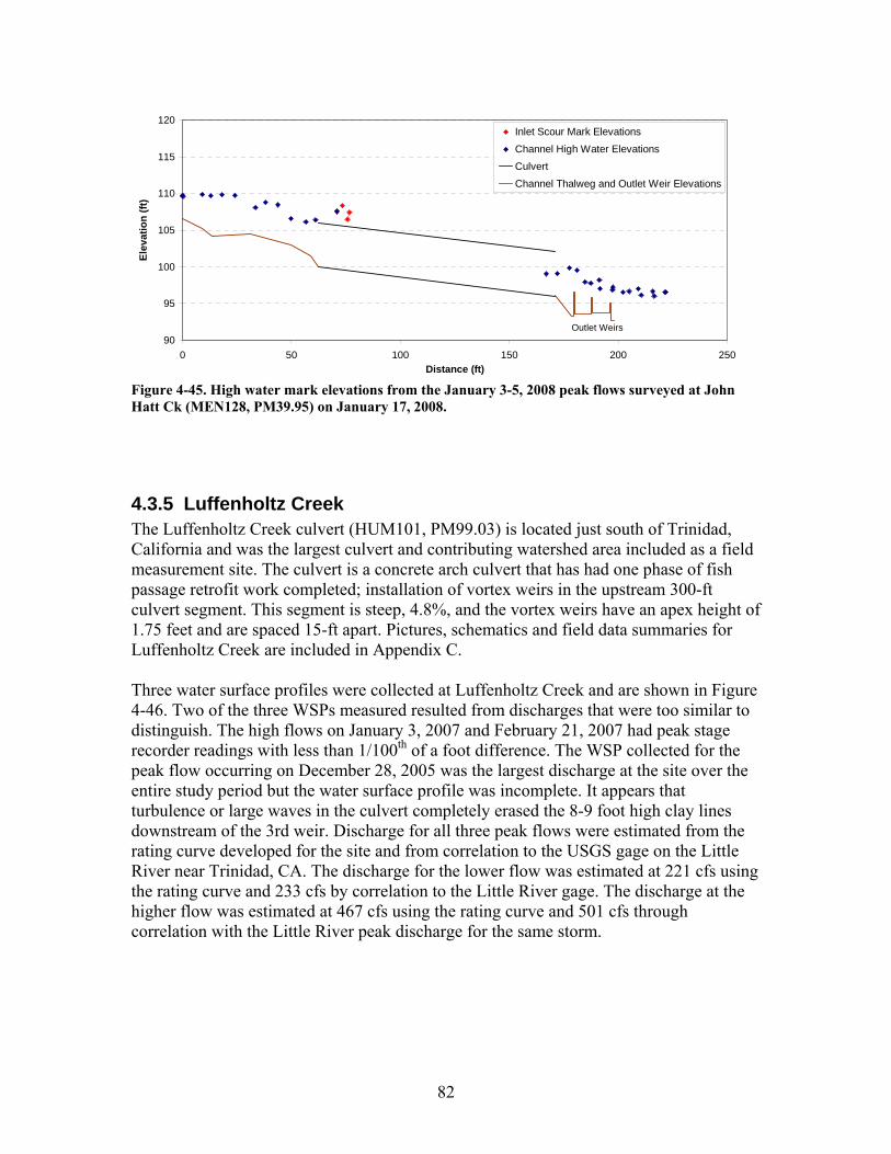
90

95

100

105

110

115

120

0 50 100 150 200 250Distance (ft)

Elev

atio

n (ft

)Inlet Scour Mark ElevationsChannel High Water ElevationsCulvertChannel Thalweg and Outlet Weir Elevations

Outlet Weirs

Figure 4-45. High water mark elevations from the January 3-5, 2008 peak flows surveyed at John Hatt Ck (MEN128, PM39.95) on January 17, 2008.

4.3.5 Luffenholtz Creek The Luffenholtz Creek culvert (HUM101, PM99.03) is located just south of Trinidad, California and was the largest culvert and contributing watershed area included as a field measurement site. The culvert is a concrete arch culvert that has had one phase of fish passage retrofit work completed; installation of vortex weirs in the upstream 300-ft culvert segment. This segment is steep, 4.8%, and the vortex weirs have an apex height of 1.75 feet and are spaced 15-ft apart. Pictures, schematics and field data summaries for Luffenholtz Creek are included in Appendix C. Three water surface profiles were collected at Luffenholtz Creek and are shown in Figure 4-46. Two of the three WSPs measured resulted from discharges that were too similar to distinguish. The high flows on January 3, 2007 and February 21, 2007 had peak stage recorder readings with less than 1/100th of a foot difference. The WSP collected for the peak flow occurring on December 28, 2005 was the largest discharge at the site over the entire study period but the water surface profile was incomplete. It appears that turbulence or large waves in the culvert completely erased the 8-9 foot high clay lines downstream of the 3rd weir. Discharge for all three peak flows were estimated from the rating curve developed for the site and from correlation to the USGS gage on the Little River near Trinidad, CA. The discharge for the lower flow was estimated at 221 cfs using the rating curve and 233 cfs by correlation to the Little River gage. The discharge at the higher flow was estimated at 467 cfs using the rating curve and 501 cfs through correlation with the Little River peak discharge for the same storm.

82

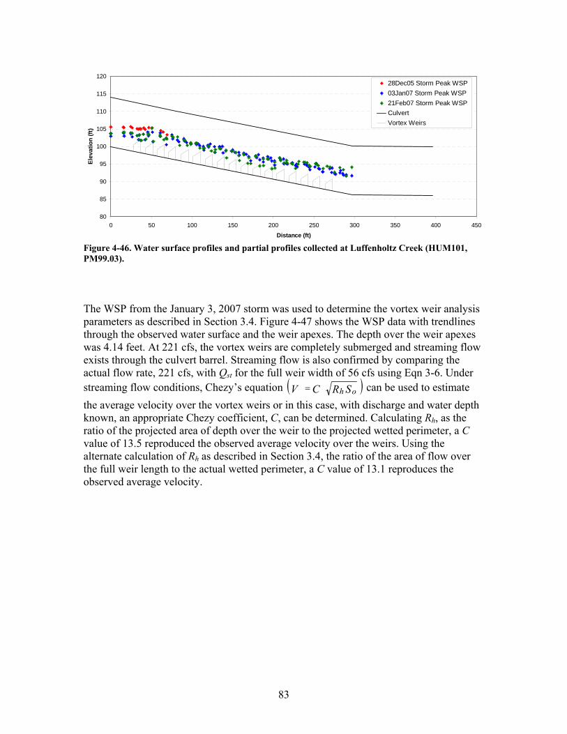
80

85

90

95

100

105

110

115

120

0 50 100 150 200 250 300 350 400 450

Distance (ft)

Elev

atio

n (ft

)28Dec05 Storm Peak WSP03Jan07 Storm Peak WSP21Feb07 Storm Peak WSPCulvertVortex Weirs

Figure 4-46. Water surface profiles and partial profiles collected at Luffenholtz Creek (HUM101, PM99.03). The WSP from the January 3, 2007 storm was used to determine the vortex weir analysis parameters as described in Section 3.4. Figure 4-47 shows the WSP data with trendlines through the observed water surface and the weir apexes. The depth over the weir apexes was 4.14 feet. At 221 cfs, the vortex weirs are completely submerged and streaming flow exists through the culvert barrel. Streaming flow is also confirmed by comparing the actual flow rate, 221 cfs, with Qst for the full weir width of 56 cfs using Eqn 3-6. Under streaming flow conditions, Chezy’s equation ( ) SRCV oh= can be used to estimate the average velocity over the vortex weirs or in this case, with discharge and water depth known, an appropriate Chezy coefficient, C, can be determined. Calculating Rh, as the ratio of the projected area of depth over the weir to the projected wetted perimeter, a C value of 13.5 reproduced the observed average velocity over the weirs. Using the alternate calculation of Rh as described in Section 3.4, the ratio of the area of flow over the full weir length to the actual wetted perimeter, a C value of 13.1 reproduces the observed average velocity.

83

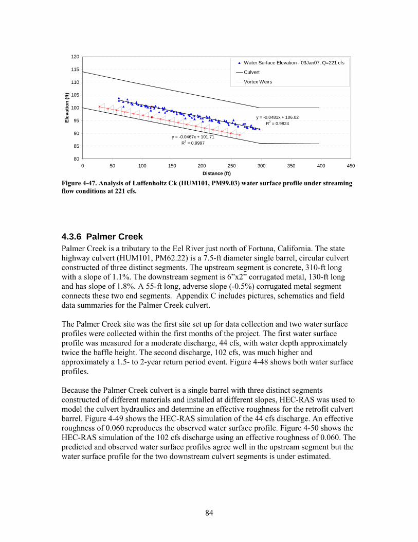
y = -0.0481x + 106.02R2 = 0.9824

y = -0.0467x + 101.71R2 = 0.9997

80

85

90

95

100

105

110

115

120

0 50 100 150 200 250 300 350 400 450Distance (ft)

Elev

atio

n (ft

)Water Surface Elevation - 03Jan07, Q=221 cfs

Culvert

Vortex Weirs

Figure 4-47. Analysis of Luffenholtz Ck (HUM101, PM99.03) water surface profile under streaming flow conditions at 221 cfs.

4.3.6 Palmer Creek Palmer Creek is a tributary to the Eel River just north of Fortuna, California. The state highway culvert (HUM101, PM62.22) is a 7.5-ft diameter single barrel, circular culvert constructed of three distinct segments. The upstream segment is concrete, 310-ft long with a slope of 1.1%. The downstream segment is 6”x2” corrugated metal, 130-ft long and has slope of 1.8%. A 55-ft long, adverse slope (-0.5%) corrugated metal segment connects these two end segments. Appendix C includes pictures, schematics and field data summaries for the Palmer Creek culvert. The Palmer Creek site was the first site set up for data collection and two water surface profiles were collected within the first months of the project. The first water surface profile was measured for a moderate discharge, 44 cfs, with water depth approximately twice the baffle height. The second discharge, 102 cfs, was much higher and approximately a 1.5- to 2-year return period event. Figure 4-48 shows both water surface profiles. Because the Palmer Creek culvert is a single barrel with three distinct segments constructed of different materials and installed at different slopes, HEC-RAS was used to model the culvert hydraulics and determine an effective roughness for the retrofit culvert barrel. Figure 4-49 shows the HEC-RAS simulation of the 44 cfs discharge. An effective roughness of 0.060 reproduces the observed water surface profile. Figure 4-50 shows the HEC-RAS simulation of the 102 cfs discharge using an effective roughness of 0.060. The predicted and observed water surface profiles agree well in the upstream segment but the water surface profile for the two downstream culvert segments is under estimated.

84

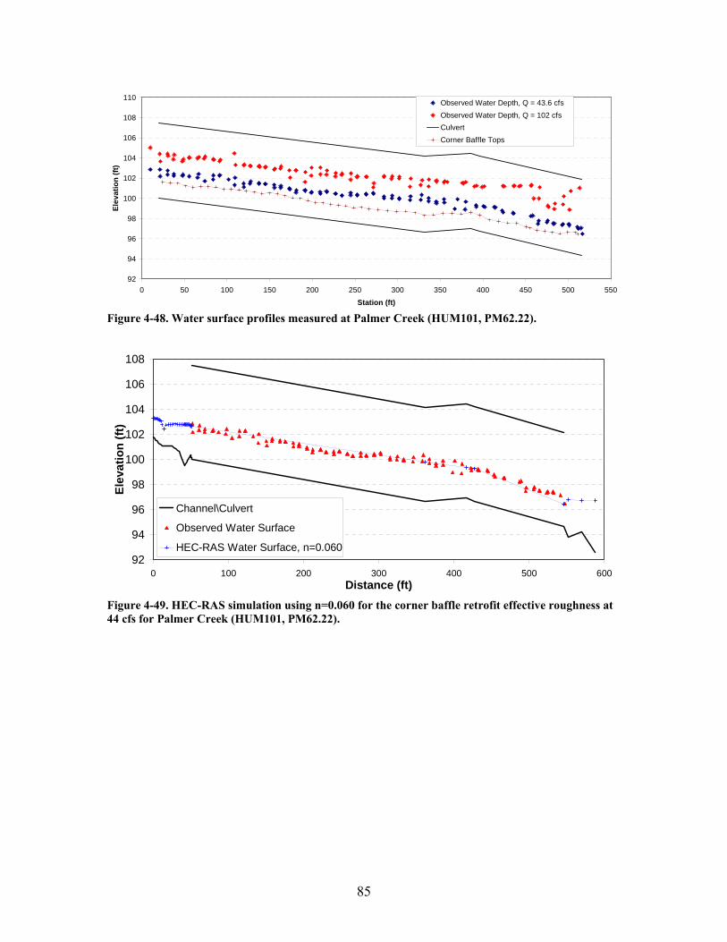
92

94

96

98

100

102

104

106

108

110

0 50 100 150 200 250 300 350 400 450 500 550

Station (ft)

Elev

atio

n (ft

)Observed Water Depth, Q = 43.6 cfsObserved Water Depth, Q = 102 cfsCulvertCorner Baffle Tops

Figure 4-48. Water surface profiles measured at Palmer Creek (HUM101, PM62.22).

92

94

96

98

100

102

104

106

108

0 100 200 300 400 500 600Distance (ft)

Elev

atio

n (ft

)

Channel\Culvert

Observed Water Surface

HEC-RAS Water Surface, n=0.060

Figure 4-49. HEC-RAS simulation using n=0.060 for the corner baffle retrofit effective roughness at 44 cfs for Palmer Creek (HUM101, PM62.22).

85

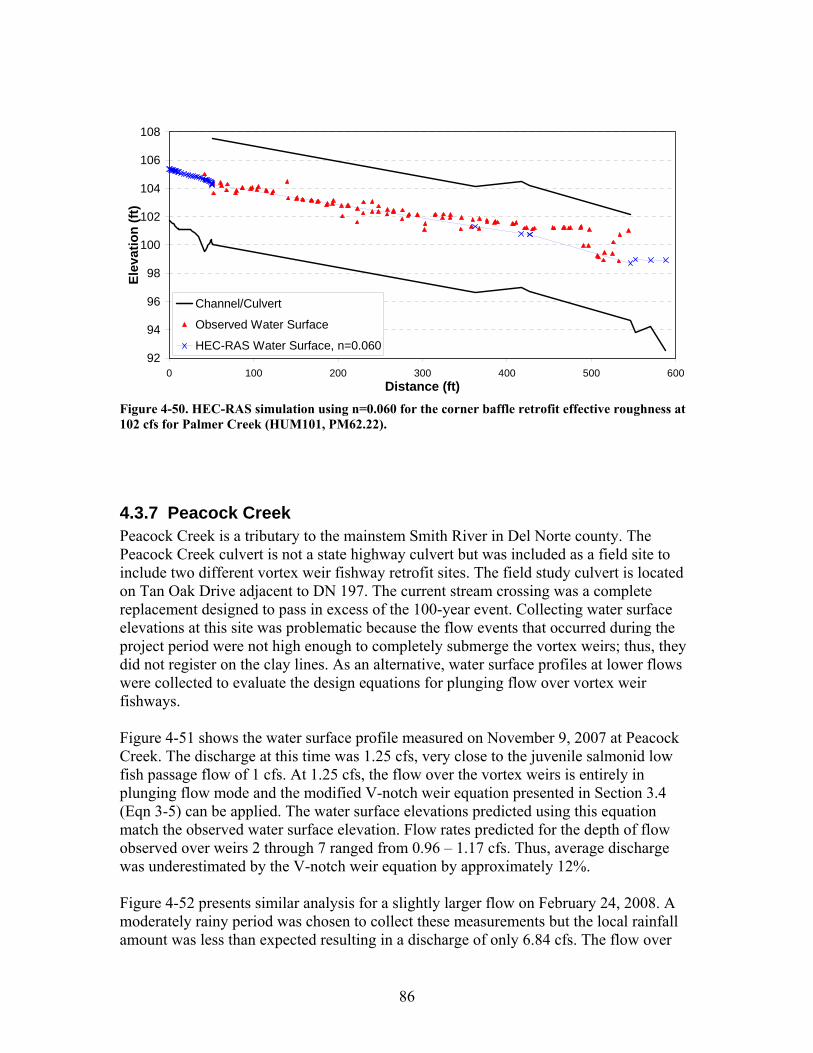
92

94

96

98

100

102

104

106

108

0 100 200 300 400 500 600Distance (ft)

Elev

atio

n (ft

)

Channel/Culvert

Observed Water Surface

HEC-RAS Water Surface, n=0.060

Figure 4-50. HEC-RAS simulation using n=0.060 for the corner baffle retrofit effective roughness at 102 cfs for Palmer Creek (HUM101, PM62.22).

4.3.7 Peacock Creek Peacock Creek is a tributary to the mainstem Smith River in Del Norte county. The Peacock Creek culvert is not a state highway culvert but was included as a field site to include two different vortex weir fishway retrofit sites. The field study culvert is located on Tan Oak Drive adjacent to DN 197. The current stream crossing was a complete replacement designed to pass in excess of the 100-year event. Collecting water surface elevations at this site was problematic because the flow events that occurred during the project period were not high enough to completely submerge the vortex weirs; thus, they did not register on the clay lines. As an alternative, water surface profiles at lower flows were collected to evaluate the design equations for plunging flow over vortex weir fishways. Figure 4-51 shows the water surface profile measured on November 9, 2007 at Peacock Creek. The discharge at this time was 1.25 cfs, very close to the juvenile salmonid low fish passage flow of 1 cfs. At 1.25 cfs, the flow over the vortex weirs is entirely in plunging flow mode and the modified V-notch weir equation presented in Section 3.4 (Eqn 3-5) can be applied. The water surface elevations predicted using this equation match the observed water surface elevation. Flow rates predicted for the depth of flow observed over weirs 2 through 7 ranged from 0.96 – 1.17 cfs. Thus, average discharge was underestimated by the V-notch weir equation by approximately 12%. Figure 4-52 presents similar analysis for a slightly larger flow on February 24, 2008. A moderately rainy period was chosen to collect these measurements but the local rainfall amount was less than expected resulting in a discharge of only 6.84 cfs. The flow over

86

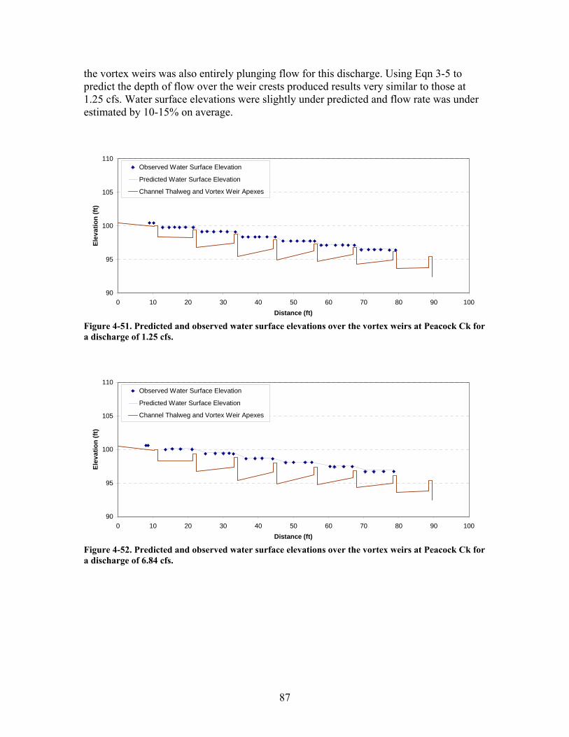
the vortex weirs was also entirely plunging flow for this discharge. Using Eqn 3-5 to predict the depth of flow over the weir crests produced results very similar to those at 1.25 cfs. Water surface elevations were slightly under predicted and flow rate was under estimated by 10-15% on average.

90

95

100

105

110

0 10 20 30 40 50 60 70 80 90 100Distance (ft)

Elev

atio

n (ft

)

Observed Water Surface Elevation

Predicted Water Surface Elevation

Channel Thalweg and Vortex Weir Apexes

Figure 4-51. Predicted and observed water surface elevations over the vortex weirs at Peacock Ck for a discharge of 1.25 cfs.

90

95

100

105

110

0 10 20 30 40 50 60 70 80 90 100Distance (ft)

Elev

atio

n (ft

)

Observed Water Surface Elevation

Predicted Water Surface Elevation

Channel Thalweg and Vortex Weir Apexes

Figure 4-52. Predicted and observed water surface elevations over the vortex weirs at Peacock Ck for a discharge of 6.84 cfs.

87

5 Discussion and Applications Section 5 presents applications and examples for design and analysis of retrofit culverts including:

• Applying the laboratory results to field-scale culvert retrofits, • Using the empirical equations and parameters presented in Section 4.1.3, • Comparing the performance of the various box culvert retrofit geometries, • Selecting model parameters and modeling approaches for design and analysis, and • Interpreting the sediment transport observations for retrofit performance.

Most of the examples provided in Section 5 use results from the full-spanning, angled baffle retrofits with the low, far-spaced and high, close-spaced baffle designs. These two cases were chosen because they have the least and greatest impact on culvert hydraulic performance. Unless otherwise indicated, all the methods presented in these examples can be applied using any of the box and circular culvert laboratory model results presented in Section 4.

5.1 Application of Laboratory Results to Field Scale Many of the laboratory results presented in Section 4 can not be applied directly to field-scale culvert retrofits. However, the laboratory-scale results can be converted to equivalent values for full-scale culverts with the same shape, and retrofits that are geometrically similar to the laboratory-scale models. Geometric similarity means that proportionality of the dimensions remains the same; e.g., the ratios of baffle height and spacing to culvert diameter or width are the same for the laboratory and field-scale culverts. Geometric similarity also requires that all slopes and angles are identical for the laboratory- and full-scale culverts. If geometric similarity requirements are met, laboratory measurements of hydraulic performance, e.g. headwater depth, or standard model parameters, such as effective roughness, can be scaled to estimate field-scale values. Direct scaling of the laboratory observations provides discrete estimates of these values for field-scale culverts operating under similar flow conditions, as defined by equivalent Froude number. Alternately, the non-dimensional empirical equations and their parameters derived from the laboratory observations can be used to make continuous predictions of field-scale retrofit culvert hydraulic performance. Both approaches are described in this section and their advantages, disadvantages and limitations are noted.

5.1.1 Headwater Elevation Impacts The headwater depth (HW) increase caused by retrofit installation in the laboratory experiments can be used to estimate HW changes for full-scale culvert retrofits. For geometrically similar culverts and retrofits, the percent HW increase observed at the laboratory scale should match the percent HW increase for a field-scale culvert at a

88

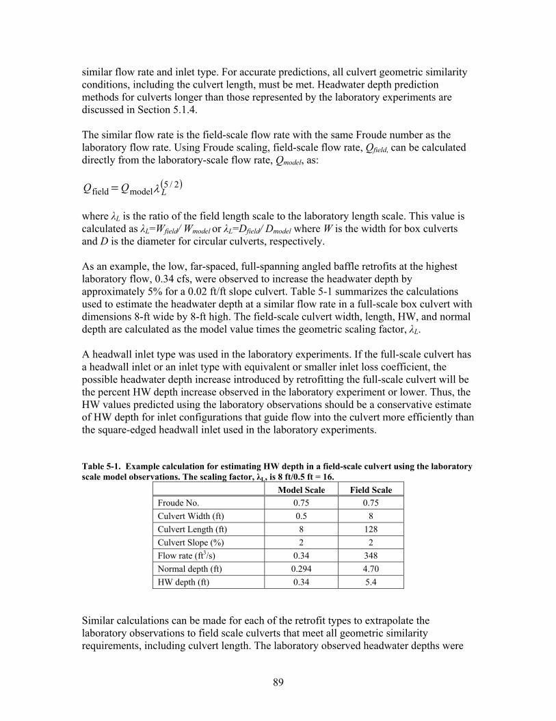
similar flow rate and inlet type. For accurate predictions, all culvert geometric similarity conditions, including the culvert length, must be met. Headwater depth prediction methods for culverts longer than those represented by the laboratory experiments are discussed in Section 5.1.4. The similar flow rate is the field-scale flow rate with the same Froude number as the laboratory flow rate. Using Froude scaling, field-scale flow rate, Qfield, can be calculated directly from the laboratory-scale flow rate, Qmodel, as:

( )λ 2/5modelfield LQQ =

where λL is the ratio of the field length scale to the laboratory length scale. This value is calculated as λL=Wfield/ Wmodel or λL=Dfield/ Dmodel where W is the width for box culverts and D is the diameter for circular culverts, respectively. As an example, the low, far-spaced, full-spanning angled baffle retrofits at the highest laboratory flow, 0.34 cfs, were observed to increase the headwater depth by approximately 5% for a 0.02 ft/ft slope culvert. Table 5-1 summarizes the calculations used to estimate the headwater depth at a similar flow rate in a full-scale box culvert with dimensions 8-ft wide by 8-ft high. The field-scale culvert width, length, HW, and normal depth are calculated as the model value times the geometric scaling factor, λL. A headwall inlet type was used in the laboratory experiments. If the full-scale culvert has a headwall inlet or an inlet type with equivalent or smaller inlet loss coefficient, the possible headwater depth increase introduced by retrofitting the full-scale culvert will be the percent HW depth increase observed in the laboratory experiment or lower. Thus, the HW values predicted using the laboratory observations should be a conservative estimate of HW depth for inlet configurations that guide flow into the culvert more efficiently than the square-edged headwall inlet used in the laboratory experiments. Table 5-1. Example calculation for estimating HW depth in a field-scale culvert using the laboratory scale model observations. The scaling factor, λL, is 8 ft/0.5 ft = 16.

Model Scale Field Scale Froude No. 0.75 0.75 Culvert Width (ft) 0.5 8 Culvert Length (ft) 8 128 Culvert Slope (%) 2 2 Flow rate (ft3/s) 0.34 348 Normal depth (ft) 0.294 4.70 HW depth (ft) 0.34 5.4

Similar calculations can be made for each of the retrofit types to extrapolate the laboratory observations to field scale culverts that meet all geometric similarity requirements, including culvert length. The laboratory observed headwater depths were

89

also compared to predicted headwater depths using the standard design equations for inlet and outlet controlled culverts in Appendix A of HDS-5 (FHWA, 2004). For the unsubmerged, inlet control equation, equation parameters for Chart 8, Nomograph scale 1 and Chart 10, Nomograph scales 1 and 3 were compared to the observed HW depth from laboratory experiments with a non-retrofit model box culvert (Figure 5-1). The Chart 10, Nomograph scale 3 parameters best reproduce the observed HW depth for the unbaffled culvert model so these parameters were used for all subsequent analyses. For the outlet control equation, the observed average water depth through the culvert barrel was used as the normal depth.

0.00

0.05

0.10

0.15

0.20

0.25

0.30

0.35

0.40

0.45

0.00 0.05 0.10 0.15 0.20 0.25 0.30 0.35 0.40Q (cfs)

HW

(ft)

Inlet Control, Chart 8, Nomograph scale 2

Inlet Control, Chart 10, Nomograph scale 1

Inlet Control, Chart 10, Nomograph scale 3

Observed HW for unbaffled model culverts

Figure 5-1. Comparison of HW depths observed in the laboratory for an unbaffled model box culvert 0.5-ft wide by 0.5-ft high to the inlet control HW prediction equations of HDS-5 (FHWA, 2004). Data includes all culvert slopes. Figure 5-2 shows the HDS-5 inlet and outlet control HW depths compared to those observed in the laboratory experiments for the low, far-spaced, full-spanning angle baffle retrofits in a box culvert. For slopes of 2% and greater, the low far-spaced retrofit culvert functions in inlet control and the retrofits have little impact on the headwater elevation. At 0.5 and 1% slopes, the culvert is in outlet control at low flows but transitions to inlet control at the higher flow rates. Figure 5-3 compares the same HW prediction equations to the laboratory experiments for the high, close-spaced, full-spanning angle baffle retrofits. For this retrofit configuration,

90

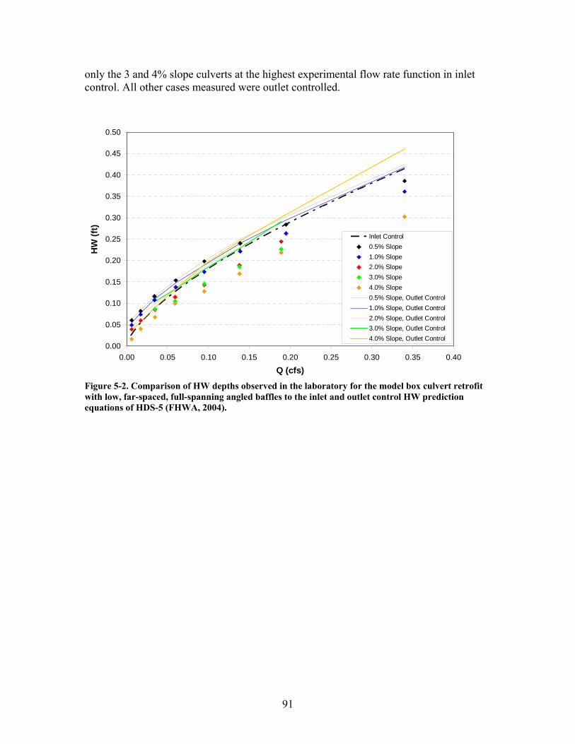
only the 3 and 4% slope culverts at the highest experimental flow rate function in inlet control. All other cases measured were outlet controlled.

0.00

0.05

0.10

0.15

0.20

0.25

0.30

0.35

0.40

0.45

0.50

0.00 0.05 0.10 0.15 0.20 0.25 0.30 0.35 0.40

Q (cfs)

HW

(ft)

Inlet Control0.5% Slope1.0% Slope2.0% Slope3.0% Slope4.0% Slope0.5% Slope, Outlet Control1.0% Slope, Outlet Control2.0% Slope, Outlet Control3.0% Slope, Outlet Control4.0% Slope, Outlet Control

Figure 5-2. Comparison of HW depths observed in the laboratory for the model box culvert retrofit with low, far-spaced, full-spanning angled baffles to the inlet and outlet control HW prediction equations of HDS-5 (FHWA, 2004).

91

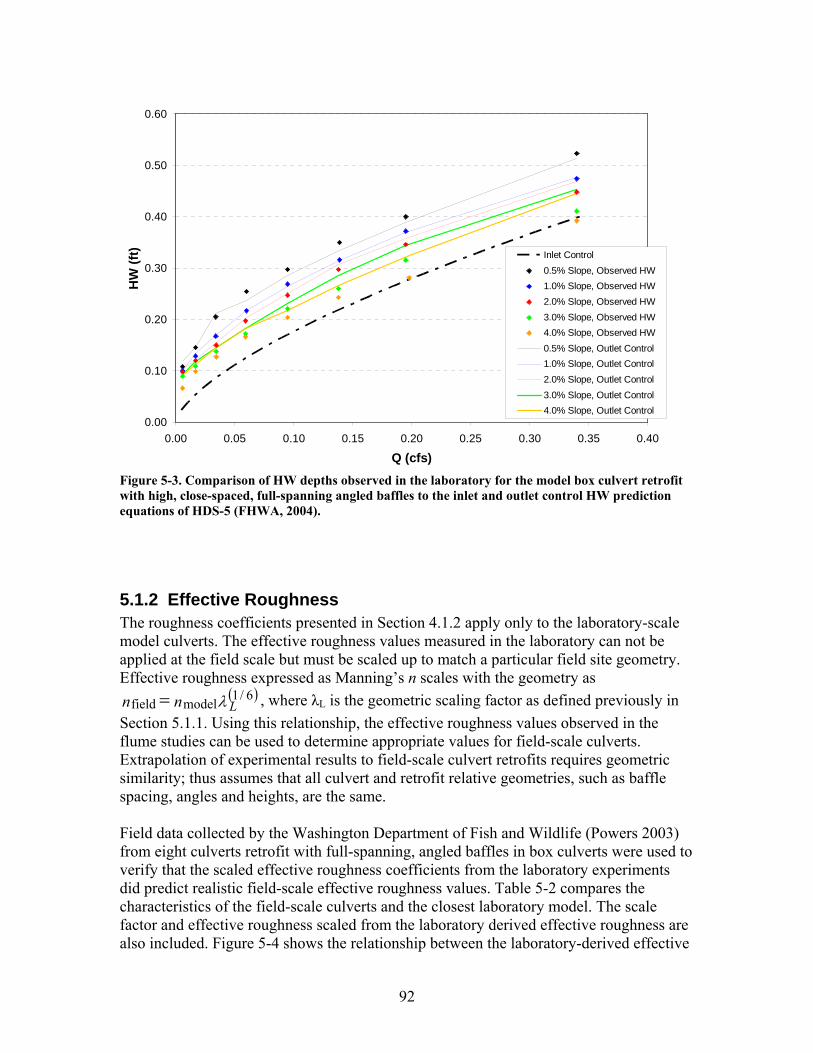
0.00

0.10

0.20

0.30

0.40

0.50

0.60

0.00 0.05 0.10 0.15 0.20 0.25 0.30 0.35 0.40

Q (cfs)

HW

(ft) Inlet Control

0.5% Slope, Observed HW1.0% Slope, Observed HW2.0% Slope, Observed HW3.0% Slope, Observed HW4.0% Slope, Observed HW0.5% Slope, Outlet Control1.0% Slope, Outlet Control2.0% Slope, Outlet Control3.0% Slope, Outlet Control4.0% Slope, Outlet Control

Figure 5-3. Comparison of HW depths observed in the laboratory for the model box culvert retrofit with high, close-spaced, full-spanning angled baffles to the inlet and outlet control HW prediction equations of HDS-5 (FHWA, 2004).

5.1.2 Effective Roughness The roughness coefficients presented in Section 4.1.2 apply only to the laboratory-scale model culverts. The effective roughness values measured in the laboratory can not be applied at the field scale but must be scaled up to match a particular field site geometry. Effective roughness expressed as Manning’s n scales with the geometry as

(λ 6/1modelfield

)Lnn = , where λL is the geometric scaling factor as defined previously in

Section 5.1.1. Using this relationship, the effective roughness values observed in the flume studies can be used to determine appropriate values for field-scale culverts. Extrapolation of experimental results to field-scale culvert retrofits requires geometric similarity; thus assumes that all culvert and retrofit relative geometries, such as baffle spacing, angles and heights, are the same. Field data collected by the Washington Department of Fish and Wildlife (Powers 2003) from eight culverts retrofit with full-spanning, angled baffles in box culverts were used to verify that the scaled effective roughness coefficients from the laboratory experiments did predict realistic field-scale effective roughness values. Table 5-2 compares the characteristics of the field-scale culverts and the closest laboratory model. The scale factor and effective roughness scaled from the laboratory derived effective roughness are also included. Figure 5-4 shows the relationship between the laboratory-derived effective

92

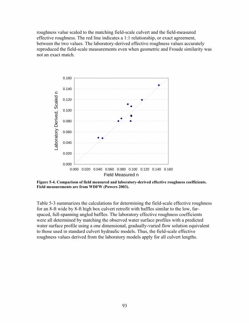
93

roughness value scaled to the matching field-scale culvert and the field-measured effective roughness. The red line indicates a 1:1 relationship, or exact agreement, between the two values. The laboratory-derived effective roughness values accurately reproduced the field-scale measurements even when geometric and Froude similarity was not an exact match.

0.000

0.020

0.040

0.060

0.080

0.100

0.120

0.140

0.160

0.

Labo

rato

ry D

eriv

ed, S

cale

d n

000 0.020 0.040 0.060 0.080 0.100 0.120 0.140 0.160Field Measured n

Figure 5-4. Comparison of field measured and laboratory-derived effective roughness coefficients. Field measurements are from WDFW (Powers 2003). Table 5-3 summarizes the calculations for determining the field-scale effective roughness for an 8-ft wide by 8-ft high box culvert retrofit with baffles similar to the low, far-spaced, full-spanning angled baffles. The laboratory effective roughness coefficients were all determined by matching the observed water surface profiles with a predicted water surface profile using a one dimensional, gradually-varied flow solution equivalent to those used in standard culvert hydraulic models. Thus, the field-scale effective roughness values derived from the laboratory models apply for all culvert lengths.

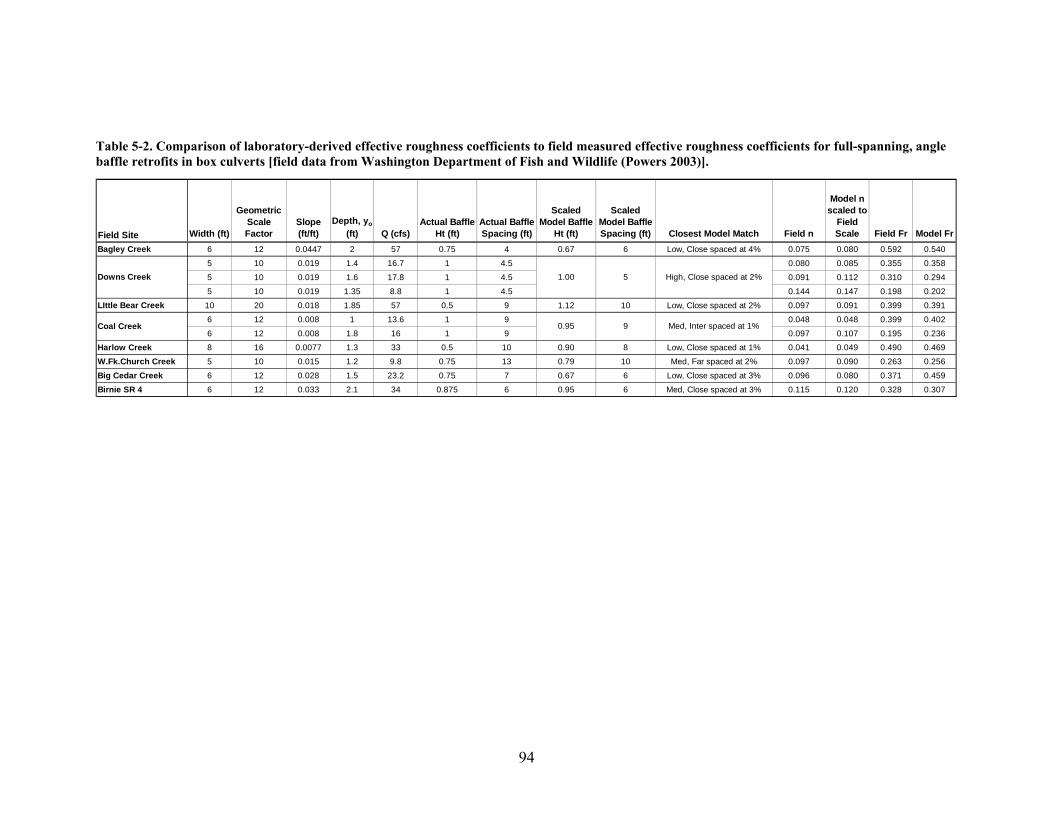
94

Table 5-2. Comparison of laboratory-derived effective roughness coefficients to field measured effective roughness coefficients for full-spanning, angle baffle retrofits in box culverts [field data from Washington Department of Fish and Wildlife (Powers 2003)].

Field Site Width (ft)

Geometric Scale Factor

Slope (ft/ft)

Depth, yo (ft) Q (cfs)

Actual Baffle Ht (ft)

Actual Baffle Spacing (ft)

Scaled Model Baffle

Ht (ft)

Scaled Model Baffle Spacing (ft) Closest Model Match Field n

Model n scaled to

Field Scale Field Fr Model Fr

Bagley Creek 6 12 0.0447 2 57 0.75 4 0.67 6 Low, Close spaced at 4% 0.075 0.080 0.592 0.540

5 10 0.019 1.4 16.7 1 4.5 0.080 0.085 0.355 0.358

5 10 0.019 1.6 17.8 1 4.5 0.091 0.112 0.310 0.294

5 10 0.019 1.35 8.8 1 4.5 0.144 0.147 0.198 0.202

LIttle Bear Creek 10 20 0.018 1.85 57 0.5 9 1.12 10 Low, Close spaced at 2% 0.097 0.091 0.399 0.391

6 12 0.008 1 13.6 1 9 0.048 0.048 0.399 0.402

6 12 0.008 1.8 16 1 9 0.097 0.107 0.195 0.236

Harlow Creek 8 16 0.0077 1.3 33 0.5 10 0.90 8 Low, Close spaced at 1% 0.041 0.049 0.490 0.469

W.Fk.Church Creek 5 10 0.015 1.2 9.8 0.75 13 0.79 10 Med, Far spaced at 2% 0.097 0.090 0.263 0.256

Big Cedar Creek 6 12 0.028 1.5 23.2 0.75 7 0.67 6 Low, Close spaced at 3% 0.096 0.080 0.371 0.459

Birnie SR 4 6 12 0.033 2.1 34 0.875 6 0.95 6 Med, Close spaced at 3% 0.115 0.120 0.328 0.307

Coal Creek Med, Inter spaced at 1%

1.00 5

90.95

High, Close spaced at 2%Downs Creek

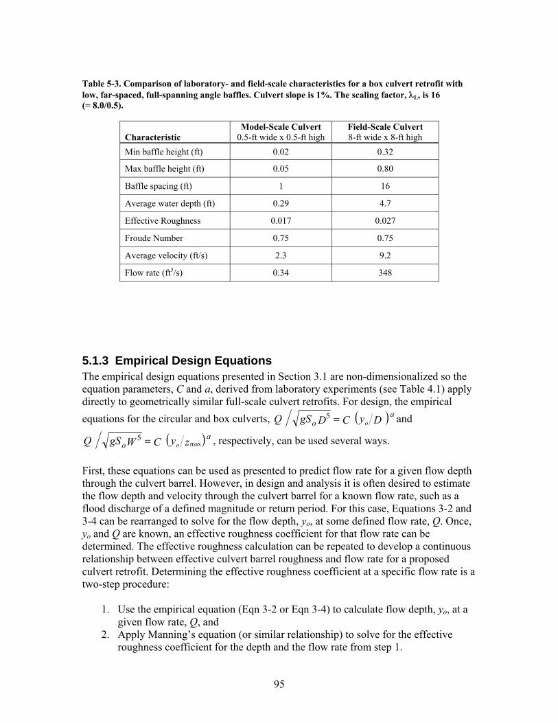
Table 5-3. Comparison of laboratory- and field-scale characteristics for a box culvert retrofit with low, far-spaced, full-spanning angle baffles. Culvert slope is 1%. The scaling factor, λL, is 16 (= 8.0/0.5).

Characteristic Model-Scale Culvert

0.5-ft wide x 0.5-ft high Field-Scale Culvert 8-ft wide x 8-ft high

Min baffle height (ft) 0.02 0.32

Max baffle height (ft) 0.05 0.80

Baffle spacing (ft) 1 16

Average water depth (ft) 0.29 4.7

Effective Roughness 0.017 0.027

Froude Number 0.75 0.75

Average velocity (ft/s) 2.3 9.2

Flow rate (ft3/s) 0.34 348

5.1.3 Empirical Design Equations The empirical design equations presented in Section 3.1 are non-dimensionalized so the equation parameters, C and a, derived from laboratory experiments (see Table 4.1) apply directly to geometrically similar full-scale culvert retrofits. For design, the empirical equations for the circular and box culverts, ( )DyCDgSQ o

ao

5 = and

( zyCWgSQ oa

o max 5 = ) , respectively, can be used several ways.

First, these equations can be used as presented to predict flow rate for a given flow depth through the culvert barrel. However, in design and analysis it is often desired to estimate the flow depth and velocity through the culvert barrel for a known flow rate, such as a flood discharge of a defined magnitude or return period. For this case, Equations 3-2 and 3-4 can be rearranged to solve for the flow depth, yo, at some defined flow rate, Q. Once, yo and Q are known, an effective roughness coefficient for that flow rate can be determined. The effective roughness calculation can be repeated to develop a continuous relationship between effective culvert barrel roughness and flow rate for a proposed culvert retrofit. Determining the effective roughness coefficient at a specific flow rate is a two-step procedure:

1. Use the empirical equation (Eqn 3-2 or Eqn 3-4) to calculate flow depth, yo, at a given flow rate, Q, and

2. Apply Manning’s equation (or similar relationship) to solve for the effective roughness coefficient for the depth and the flow rate from step 1.

95

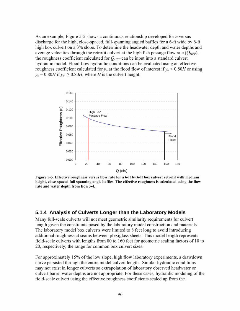
As an example, Figure 5-5 shows a continuous relationship developed for n versus discharge for the high, close-spaced, full-spanning angled baffles for a 6-ft wide by 6-ft high box culvert on a 3% slope. To determine the headwater depth and water depths and average velocities through the retrofit culvert at the high fish passage flow rate (QHFP), the roughness coefficient calculated for QHFP can be input into a standard culvert hydraulic model. Flood flow hydraulic conditions can be evaluated using an effective roughness coefficient calculated for yo at the flood flow of interest if yo < 0.80H or using yo = 0.80H if yo ≥ 0.80H, where H is the culvert height.

0.000

0.020

0.040

0.060

0.080

0.100

0.120

0.140

0.160

0 20 40 60 80 100 120 140 160 180

Q (cfs)

Effe

ctiv

e R

ough

ness

(n)

High Fish Passage Flow

Flood Flows

Figure 5-5. Effective roughness versus flow rate for a 6-ft by 6-ft box culvert retrofit with medium height, close-spaced full spanning angle baffles. The effective roughness is calculated using the flow rate and water depth from Eqn 3-4.

5.1.4 Analysis of Culverts Longer than the Laboratory Models Many full-scale culverts will not meet geometric similarity requirements for culvert length given the constraints posed by the laboratory model construction and materials. The laboratory model box culverts were limited to 8 feet long to avoid introducing additional roughness at seams between plexiglass sheets. This model length represents field-scale culverts with lengths from 80 to 160 feet for geometric scaling factors of 10 to 20, respectively; the range for common box culvert sizes. For approximately 15% of the low slope, high flow laboratory experiments, a drawdown curve persisted through the entire model culvert length. Similar hydraulic conditions may not exist in longer culverts so extrapolation of laboratory observed headwater or culvert barrel water depths are not appropriate. For these cases, hydraulic modeling of the field-scale culvert using the effective roughness coefficients scaled up from the

96

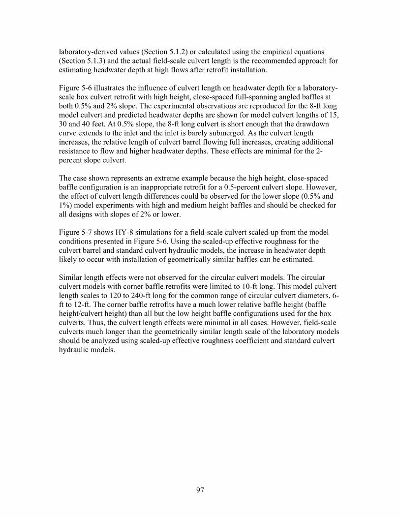
laboratory-derived values (Section 5.1.2) or calculated using the empirical equations (Section 5.1.3) and the actual field-scale culvert length is the recommended approach for estimating headwater depth at high flows after retrofit installation. Figure 5-6 illustrates the influence of culvert length on headwater depth for a laboratory-scale box culvert retrofit with high height, close-spaced full-spanning angled baffles at both 0.5% and 2% slope. The experimental observations are reproduced for the 8-ft long model culvert and predicted headwater depths are shown for model culvert lengths of 15, 30 and 40 feet. At 0.5% slope, the 8-ft long culvert is short enough that the drawdown curve extends to the inlet and the inlet is barely submerged. As the culvert length increases, the relative length of culvert barrel flowing full increases, creating additional resistance to flow and higher headwater depths. These effects are minimal for the 2-percent slope culvert. The case shown represents an extreme example because the high height, close-spaced baffle configuration is an inappropriate retrofit for a 0.5-percent culvert slope. However, the effect of culvert length differences could be observed for the lower slope (0.5% and 1%) model experiments with high and medium height baffles and should be checked for all designs with slopes of 2% or lower. Figure 5-7 shows HY-8 simulations for a field-scale culvert scaled-up from the model conditions presented in Figure 5-6. Using the scaled-up effective roughness for the culvert barrel and standard culvert hydraulic models, the increase in headwater depth likely to occur with installation of geometrically similar baffles can be estimated. Similar length effects were not observed for the circular culvert models. The circular culvert models with corner baffle retrofits were limited to 10-ft long. This model culvert length scales to 120 to 240-ft long for the common range of circular culvert diameters, 6-ft to 12-ft. The corner baffle retrofits have a much lower relative baffle height (baffle height/culvert height) than all but the low height baffle configurations used for the box culverts. Thus, the culvert length effects were minimal in all cases. However, field-scale culverts much longer than the geometrically similar length scale of the laboratory models should be analyzed using scaled-up effective roughness coefficient and standard culvert hydraulic models.

97

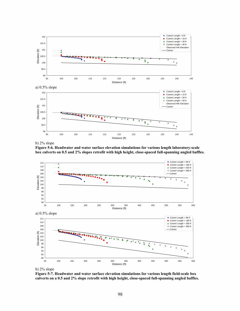
99

99.5

100

100.5

101

101.5

102

95 100 105 110 115 120 125 130 135 140 145

Distance (ft)

Elev

atio

n (ft

)Culvert Length = 8 ftCulvert Length = 15 ftCulvert Length = 30 ftCulvert Length = 40 ftObserved HW ElevationCulvert

a) 0.5% slope

99

99.5

100

100.5

101

101.5

102

95 100 105 110 115 120 125 130 135 140 145

Distance (ft)

Elev

atio

n (ft

)

Culvert Length = 8 ftCulvert Length = 15 ftCulvert Length = 30 ftCulvert Length = 40 ftObserved HW ElevationCulvert

b) 2% slope Figure 5-6. Headwater and water surface elevation simulations for various length laboratory-scale box culverts on 0.5 and 2% slopes retrofit with high height, close-spaced full-spanning angled baffles.

90

92

94

96

98

100

102

104

106

108

110

112

50 100 150 200 250 300 350 400 450 500 550 600Distance (ft)

Ele

vatio

n (ft

)

Culvert Length = 96 ftCulvert Length = 180 ftCulvert Length = 350 ftCulvert Length = 480 ftCulvert

a) 0.5% slope

90

92

94

96

98

100

102

104

106

108

110

112

50 100 150 200 250 300 350 400 450 500 550 600Distance (ft)

Elev

atio

n (ft

)

Culvert Length = 96 ftCulvert Length = 180 ftCulvert Length = 350 ftCulvert Length = 480 ftCulvert

b) 2% slope Figure 5-7. Headwater and water surface elevation simulations for various length field-scale box culverts on a 0.5 and 2% slope retrofit with high height, close-spaced full-spanning angled baffles.

98

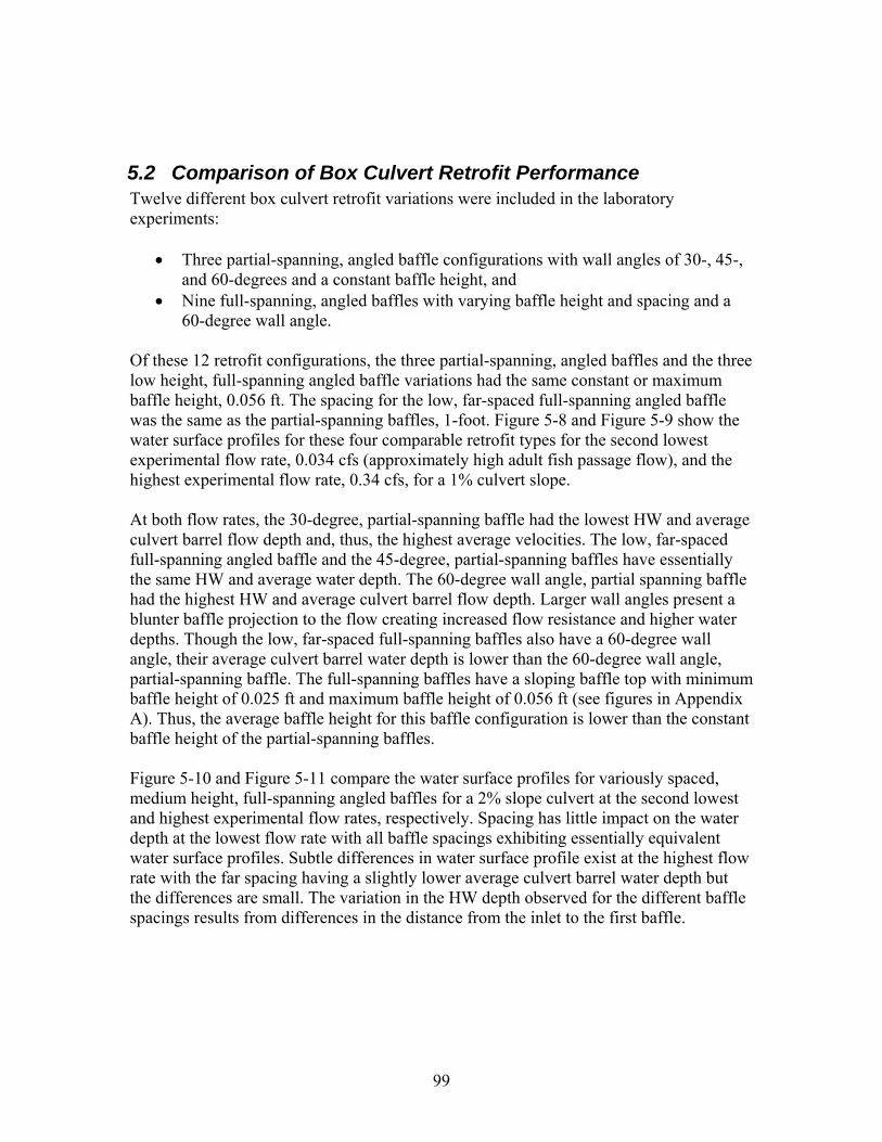
5.2 Comparison of Box Culvert Retrofit Performance Twelve different box culvert retrofit variations were included in the laboratory experiments:

• Three partial-spanning, angled baffle configurations with wall angles of 30-, 45-, and 60-degrees and a constant baffle height, and

• Nine full-spanning, angled baffles with varying baffle height and spacing and a 60-degree wall angle.

Of these 12 retrofit configurations, the three partial-spanning, angled baffles and the three low height, full-spanning angled baffle variations had the same constant or maximum baffle height, 0.056 ft. The spacing for the low, far-spaced full-spanning angled baffle was the same as the partial-spanning baffles, 1-foot. Figure 5-8 and Figure 5-9 show the water surface profiles for these four comparable retrofit types for the second lowest experimental flow rate, 0.034 cfs (approximately high adult fish passage flow), and the highest experimental flow rate, 0.34 cfs, for a 1% culvert slope. At both flow rates, the 30-degree, partial-spanning baffle had the lowest HW and average culvert barrel flow depth and, thus, the highest average velocities. The low, far-spaced full-spanning angled baffle and the 45-degree, partial-spanning baffles have essentially the same HW and average water depth. The 60-degree wall angle, partial spanning baffle had the highest HW and average culvert barrel flow depth. Larger wall angles present a blunter baffle projection to the flow creating increased flow resistance and higher water depths. Though the low, far-spaced full-spanning baffles also have a 60-degree wall angle, their average culvert barrel water depth is lower than the 60-degree wall angle, partial-spanning baffle. The full-spanning baffles have a sloping baffle top with minimum baffle height of 0.025 ft and maximum baffle height of 0.056 ft (see figures in Appendix A). Thus, the average baffle height for this baffle configuration is lower than the constant baffle height of the partial-spanning baffles. Figure 5-10 and Figure 5-11 compare the water surface profiles for variously spaced, medium height, full-spanning angled baffles for a 2% slope culvert at the second lowest and highest experimental flow rates, respectively. Spacing has little impact on the water depth at the lowest flow rate with all baffle spacings exhibiting essentially equivalent water surface profiles. Subtle differences in water surface profile exist at the highest flow rate with the far spacing having a slightly lower average culvert barrel water depth but the differences are small. The variation in the HW depth observed for the different baffle spacings results from differences in the distance from the inlet to the first baffle.

99

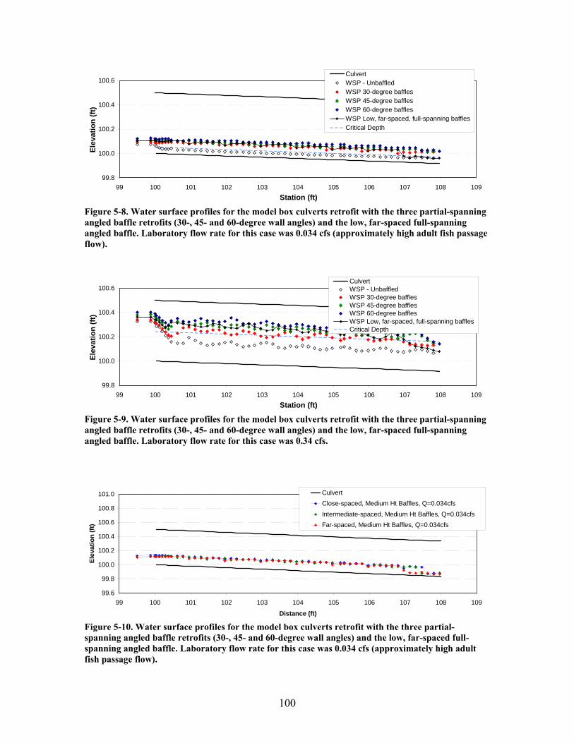
99.8

100.0

100.2

100.4

100.6

99 100 101 102 103 104 105 106 107 108 109Station (ft)

Elev

atio

n (ft

)

CulvertWSP - UnbaffledWSP 30-degree bafflesWSP 45-degree bafflesWSP 60-degree bafflesWSP Low, far-spaced, full-spanning bafflesCritical Depth

Figure 5-8. Water surface profiles for the model box culverts retrofit with the three partial-spanning angled baffle retrofits (30-, 45- and 60-degree wall angles) and the low, far-spaced full-spanning angled baffle. Laboratory flow rate for this case was 0.034 cfs (approximately high adult fish passage flow).

99.8

100.0

100.2

100.4

100.6

99 100 101 102 103 104 105 106 107 108 109Station (ft)

Elev

atio

n (ft

)

CulvertWSP - UnbaffledWSP 30-degree bafflesWSP 45-degree bafflesWSP 60-degree bafflesWSP Low, far-spaced, full-spanning bafflesCritical Depth

Figure 5-9. Water surface profiles for the model box culverts retrofit with the three partial-spanning angled baffle retrofits (30-, 45- and 60-degree wall angles) and the low, far-spaced full-spanning angled baffle. Laboratory flow rate for this case was 0.34 cfs.

99.6

99.8

100.0

100.2

100.4

100.6

100.8

101.0

99 100 101 102 103 104 105 106 107 108 109

Distance (ft)

Elev

atio

n (ft

)

CulvertClose-spaced, Medium Ht Baffles, Q=0.034cfsIntermediate-spaced, Medium Ht Baffles, Q=0.034cfsFar-spaced, Medium Ht Baffles, Q=0.034cfs

Figure 5-10. Water surface profiles for the model box culverts retrofit with the three partial-spanning angled baffle retrofits (30-, 45- and 60-degree wall angles) and the low, far-spaced full-spanning angled baffle. Laboratory flow rate for this case was 0.034 cfs (approximately high adult fish passage flow).

100

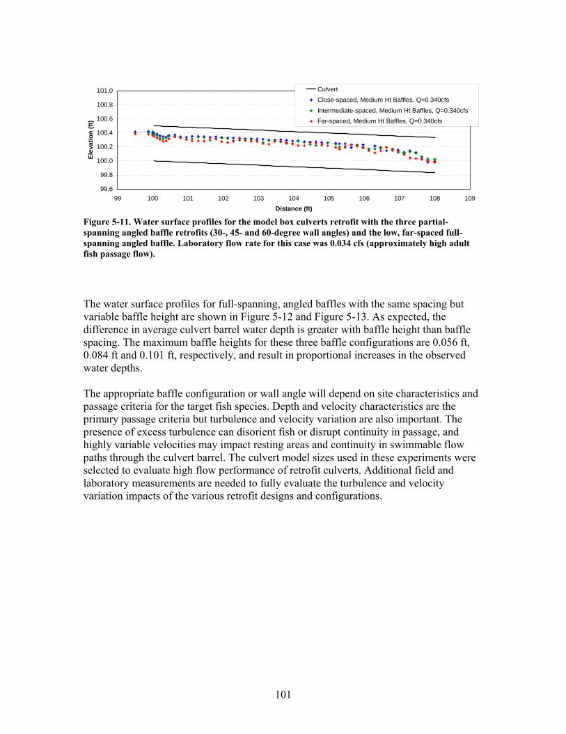
99.6

99.8

100.0

100.2

100.4

100.6

100.8

101.0

99 100 101 102 103 104 105 106 107 108 109Distance (ft)

Elev

atio

n (ft

)CulvertClose-spaced, Medium Ht Baffles, Q=0.340cfsIntermediate-spaced, Medium Ht Baffles, Q=0.340cfsFar-spaced, Medium Ht Baffles, Q=0.340cfs

Figure 5-11. Water surface profiles for the model box culverts retrofit with the three partial-spanning angled baffle retrofits (30-, 45- and 60-degree wall angles) and the low, far-spaced full-spanning angled baffle. Laboratory flow rate for this case was 0.034 cfs (approximately high adult fish passage flow). The water surface profiles for full-spanning, angled baffles with the same spacing but variable baffle height are shown in Figure 5-12 and Figure 5-13. As expected, the difference in average culvert barrel water depth is greater with baffle height than baffle spacing. The maximum baffle heights for these three baffle configurations are 0.056 ft, 0.084 ft and 0.101 ft, respectively, and result in proportional increases in the observed water depths. The appropriate baffle configuration or wall angle will depend on site characteristics and passage criteria for the target fish species. Depth and velocity characteristics are the primary passage criteria but turbulence and velocity variation are also important. The presence of excess turbulence can disorient fish or disrupt continuity in passage, and highly variable velocities may impact resting areas and continuity in swimmable flow paths through the culvert barrel. The culvert model sizes used in these experiments were selected to evaluate high flow performance of retrofit culverts. Additional field and laboratory measurements are needed to fully evaluate the turbulence and velocity variation impacts of the various retrofit designs and configurations.

101

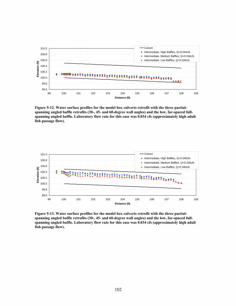
99.6

99.8

100.0

100.2

100.4

100.6

100.8

101.0

99 100 101 102 103 104 105 106 107 108 109Distance (ft)

Elev

atio

n (ft

)

CulvertIntermediate, High Baffles, Q=0.034cfsIntermediate, Medium Baffles, Q=0.034cfsIntermediate, Low Baffles, Q=0.034cfs

Figure 5-12. Water surface profiles for the model box culverts retrofit with the three partial-spanning angled baffle retrofits (30-, 45- and 60-degree wall angles) and the low, far-spaced full-spanning angled baffle. Laboratory flow rate for this case was 0.034 cfs (approximately high adult fish passage flow).

99.6

99.8

100.0

100.2

100.4

100.6

100.8

101.0

99 100 101 102 103 104 105 106 107 108 109Distance (ft)

Elev

atio

n (ft

)

CulvertIntermediate, High Baffles, Q=0.340cfsIntermediate, Medium Baffles, Q=0.340cfsIntermediate, Low Baffles, Q=0.340cfs

Figure 5-13. Water surface profiles for the model box culverts retrofit with the three partial-spanning angled baffle retrofits (30-, 45- and 60-degree wall angles) and the low, far-spaced full-spanning angled baffle. Laboratory flow rate for this case was 0.034 cfs (approximately high adult fish passage flow).

102

5.3 Modeling Approaches for Design and Analysis Hydraulic performance of a culvert retrofit must be analyzed at both fish passage and flood discharges. Fish passage flow rates are typically defined as a low and high fish passage flow for each target fish species or age-class of interest. The model sizes used in the flume experiments were selected to analyze retrofit culvert performance at flood flows. Thus, the results and approaches here are not applicable over the full range of flows needed to analyze fish passage performance. However, the results do apply over some range of the fish passage flow rates. This section describes how to determine the applicability of these results at a particular discharge and describes recommended analysis procedures. The lower flow rate for which the flume experimental results apply is the flow rate at which streaming flow begins. This flow rate can be identified using the following procedure:

1. Identify the appropriate baffle configuration (e.g. baffle height and spacing) for a proposed retrofit.

2. Calculate the water depth, yo, at the initiation of streaming flow. For corner baffle retrofits in circular culverts, streaming flows exists at lower relative depths, approximately yo = 0.75*zmax (see Figure 3-2 for definitions of zmax). For box culverts retrofit with either angled baffle design, streaming flow is assumed to exist when the water depth is greater than or equal to 1.1 times the maximum baffle height, or yo = 1.1*zmax (see Figure 3-1 for definitions of zmax).

3. Use the empirical design equations (Eqn 3-2 for circular culverts with corner

baffles or Eqn 3-4 for box culverts with angled baffles) and appropriate parameter values (Table 4-1) for the selected baffle design to calculate Q given yo from step 2.

This is the lowest flow rate at which the analysis procedures presented here can be applied. High fish passage flows are determined from hydrologic analysis at the site of interest and these flows generally create streaming flow conditions. Once the high fish passage flow is determined for the target fish species or age-classes, applicability of the flume experiment results can be determined. This procedure is summarized by the following steps:

103

1. Determine the high fish passage flow (QHFP) through hydrologic analysis (see CDFG 2003)

2. Use Eqn 3-2 for circular culverts with corner baffles or Eqn 3-4 for box culverts with angled baffles and the appropriate equation parameters (Table 4-1) to calculate yo at QHFP.

3. Compare yo to the maximum baffle height to confirm that streaming flow exists. For corner baffle retrofits in circular culverts, if yo ≥ 0.75 times the maximum baffle height, zmax, the methods presented here apply and can be used for analysis For box culverts with angled baffle retrofits, if yo ≥ 1.1 times the maximum baffle height, zmax, the methods presented here apply and can be used for analysis

4. Calculate the roughness coefficient at high fish passage flow by rearranging Manning’s equation to solve for n using yo at QHFP.

5. The hydraulic performance of the retrofit culvert at the high fish passage flow can now be conducted using standard culvert analysis software and the effective roughness coefficient at QHFP.

Design flood flows and other high discharges of interest are determined using standard hydrologic methods. Once the discharges of interest are identified, a procedure similar to the analysis of the high fish passage flow can be used to determine a roughness coefficient at each discharge for use in standard culvert analysis software. The specific procedure is outlined below.

1. Determine the flood or high flow discharges of interest using standard hydrological methods.

2. Use Eqn 3-2 for circular culverts with corner baffles or Eqn 3-4 for box culverts with angled baffles and the appropriate equation parameters (Table 4-1) to calculate yo at each of these discharges. If yo is less than or equal to 0.80*H use this yo to determine the roughness coefficient. If yo is greater than 0.80*H, use yo at 0.80*H to determine the roughness coefficient for hydraulic analysis.

3. Calculate the roughness coefficient at each discharge of interest by rearranging Manning’s equation to solve for n using yo at each discharge.

4. The hydraulic performance of the retrofit culvert at each high flow can now be conducted using standard culvert analysis software and the discharge specific effective roughness coefficient.

104

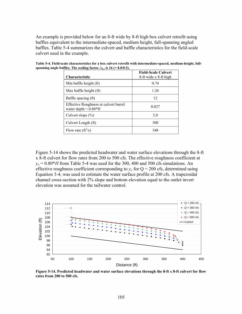
An example is provided below for an 8-ft wide by 8-ft high box culvert retrofit using baffles equivalent to the intermediate-spaced, medium height, full-spanning angled baffles. Table 5-4 summarizes the culvert and baffle characteristics for the field-scale culvert used in the example. Table 5-4. Field-scale characteristics for a box culvert retrofit with intermediate-spaced, medium-height, full-spanning angle baffles. The scaling factor, λL, is 16 (= 8.0/0.5).

Characteristic Field-Scale Culvert 8-ft wide x 8-ft high

Min baffle height (ft) 0.74

Max baffle height (ft) 1.26

Baffle spacing (ft) 12 Effective Roughness at culvert barrel water depth = 0.80*H 0.027

Culvert slope (%) 2.0

Culvert Length (ft) 300

Flow rate (ft3/s) 348 Figure 5-14 shows the predicted headwater and water surface elevations through the 8-ft x 8-ft culvert for flow rates from 200 to 500 cfs. The effective roughness coefficient at yo = 0.80*H from Table 5-4 was used for the 300, 400 and 500 cfs simulations. An effective roughness coefficient corresponding to yo for Q = 200 cfs, determined using Equation 3-4, was used to estimate the water surface profile at 200 cfs. A trapezoidal channel cross-section with 2% slope and bottom elevation equal to the outlet invert elevation was assumed for the tailwater control.

92949698

100102104106108110112114

50 100 150 200 250 300 350 400 450

Distance (ft)

Ele

vatio

n (ft

)

Q = 200 cfs

Q = 300 cfs

Q = 400 cfs

Q = 500 cfs

Culvert

Figure 5-14. Predicted headwater and water surface elevations through the 8-ft x 8-ft culvert for flow rates from 200 to 500 cfs.

105

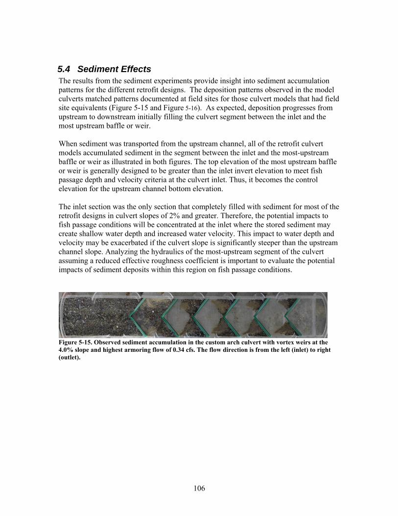
5.4 Sediment Effects The results from the sediment experiments provide insight into sediment accumulation patterns for the different retrofit designs. The deposition patterns observed in the model culverts matched patterns documented at field sites for those culvert models that had field site equivalents (Figure 5-15 and Figure 5-16). As expected, deposition progresses from upstream to downstream initially filling the culvert segment between the inlet and the most upstream baffle or weir. When sediment was transported from the upstream channel, all of the retrofit culvert models accumulated sediment in the segment between the inlet and the most-upstream baffle or weir as illustrated in both figures. The top elevation of the most upstream baffle or weir is generally designed to be greater than the inlet invert elevation to meet fish passage depth and velocity criteria at the culvert inlet. Thus, it becomes the control elevation for the upstream channel bottom elevation. The inlet section was the only section that completely filled with sediment for most of the retrofit designs in culvert slopes of 2% and greater. Therefore, the potential impacts to fish passage conditions will be concentrated at the inlet where the stored sediment may create shallow water depth and increased water velocity. This impact to water depth and velocity may be exacerbated if the culvert slope is significantly steeper than the upstream channel slope. Analyzing the hydraulics of the most-upstream segment of the culvert assuming a reduced effective roughness coefficient is important to evaluate the potential impacts of sediment deposits within this region on fish passage conditions.

Figure 5-15. Observed sediment accumulation in the custom arch culvert with vortex weirs at the 4.0% slope and highest armoring flow of 0.34 cfs. The flow direction is from the left (inlet) to right (outlet).

106

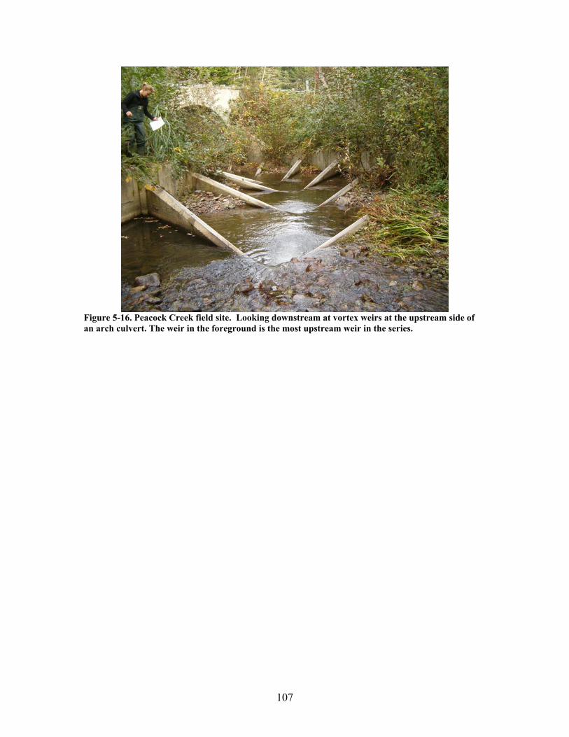
Figure 5-16. Peacock Creek field site. Looking downstream at vortex weirs at the upstream side of an arch culvert. The weir in the foreground is the most upstream weir in the series.

107

6 Summary Laboratory and field analysis of the effects of fish passage retrofits, such as baffles and weirs, on culvert hydraulic performance have primarily focused on whether the retrofit meets the hydraulic conditions needed for fish passage over the range of flows at which fish are present and attempting to migrate. Retrofitting a culvert barrel to improve fish passage may also alter the hydraulic performance of the culvert at all flows. This study was conducted to specifically measure and quantify the impact of specific retrofit designs on culvert hydraulic capacity at flood flows. Laboratory and field measurements were collected to quantify high flow hydraulic performance of retrofit culverts, develop model parameters, and identify appropriate design and analysis methods. The recommended procedure for analyzing a culvert’s hydraulic capacity after installation of culvert barrel retrofits is to use the empirical equations for a particular retrofit type as presented here for box culverts and circular culverts with corner baffles or elsewhere (e.g., Rajaratnam et al., 1988; Rajaratnam et al., 1989; Rajaratnam and Katapodis, 1990; Rajaratnam et al., 1990; Rajaratnam et al., 1991) to determine a roughness coefficient for the flow rate of interest. This roughness coefficient is then used in standard culvert hydraulic models with the specific site characteristics (e.g. inlet type, tailwater conditions, etc.) to evaluate the retrofit culvert’s hydraulic performance. The empirical equations provide effective roughness coefficients estimated over a continuous range of flows rather than the discrete flows for which laboratory measurements were collected. This approach is described in Section 5.3. Additional observations and recommendations: • Headwater Depth Impacts

Increases in the headwater depth caused by baffle or weir installation are a function of the baffle height and spacing, and the distance from the inlet to the most upstream baffle. Using the minimum baffle height and maximum baffle spacing required to meet fish passage criteria creates the least impact on headwater depth at high flows. At culvert slopes, greater than 2%, most of the retrofit culvert models functioned in inlet control at high flows.

• Influence of slope and retrofit geometry on sediment trapping Sediment was most effectively trapped in culvert barrels retrofit with closely spaced, high height baffles, and the amount of sediment trapped decreased with increasing culvert slope. For all the baffle configurations evaluated, sediment was first trapped near the inlet and either slowly filled the downstream pools between baffles or the downstream pools between the baffles did not accumulate significant sediment.

• Effects of sediment on hydraulic performance If a baffle configuration effectively traps sediment such that the pools between baffles

108

fill, the baffles are no longer effective and the culvert barrel roughness decreases significantly. This condition creates shallow water depths and fast velocities that may fail to meet fish passage criteria. These conditions were most likely to occur for high height, closely spaced baffle configurations. As the culvert slope increased, the tendency to accumulate sediment decreased because more energy was available for sediment clearing. In many cases, the culvert inlet was significantly impacted by sediment even when the rest of the retrofit culvert barrel remained clear. This occurs because the most upstream baffle acts as the bed elevation control for the upstream channel. After baffle installation, sediment is transported into the culvert barrel and fills the culvert bottom between the inlet and the first baffle to a depth equal to the baffle height. This sediment effectively reduces the inlet cross sectional area and may create a zone of shallow, high velocity water that impedes fish passage. This inlet condition should be anticipated and its potential fish passage impacts evaluated when designing and evaluating a culvert retrofit with baffles or weirs.

109

7 References Ackers, J.C., Butler, D., and May, R. W.P. 1996. “Design of sewers to control sediment problems,” CIRIA Rep. 141, Construction Industry Research and Information Association, London. Alaska Department of Fish and Game (ADFG) and Alaska Department of Transportation (ADOT). 2001. MEMORANDUM OF AGREEMENT BETWEEN ALASKA DEPARTMENT OF FISH AND GAME AND ALASKA DEPARTMENT OF TRANSPORTATION AND PUBLIC FACILITIES FOR THE DESIGN, PERMITTING, AND CONSTRUCTION OF CULVERTS FOR FISH PASSAGE http://www.dot.state.ak.us/stwddes/dcsenviron/assets/pdf/procedures/dot_adfg_fishpass080301.pdf American Fisheries Society Bioengineering Section - Fish passage mailing list archive July 2005. http://lists.oregonstate.edu/pipermail/fishpass/ Baker, C. O. and F. E. Votapka. 1990. Fish passage through culverts. USDA – Forest Service, Report No. FHWA-FL-90-0006. Bates, K. 2001. Fishway Design Guidelines for Pacific Salmon. Working paper 1.6 9/2001 Washington Department of Fish and Wildlife (WDFW). British Columbia Ministry of Forests. 2002. Fish-stream crossing guidebook. For. Prac. Br., Min. For., Victoria, B.C. Forest Practices Code of British Columbia guidebook. http://www.for.gov.bc.ca/tasb/legsregs/fpc/FPCGUIDE/FishStreamCrossing/FSCGdBk.pdf Butler, D., J. C. Ackers, and R. W. P. May. 1996. “ Sediment transport in sewers, Part 1: Background.” Proceedings, Instn. Civ. Engrs. Wat, Marit. And Energy, 118, June, 103-112. California Department of Transportation (CalTrans). 2007. Fish Passage Design for Road Crossings. http://www.dot.ca.gov/hq/oppd/fishPassage/index.htm California Department of Fish and Game (CDFG). 2002. Culvert criteria for fish passage. Sacramento, CA. 15 p. http://www.dfg.ca.gov/nafwb/pubs/2002/culvert_criteria.pdf California Department of Fish and Game (CDFG). 1998. California Salmonid Stream Habitat Restoration Manual. http://www.dot.ca.gov/hq/oppd/fishPassage/index.htm Cederholm, C.J. and W.J. Scarlett. 1981. Seasonal immigrations of juvenile salmonids into four small tributaries of the Clearwater River, Washington, 1977-1981, p. 98-110. In E.L. Brannon and E.O. Salo, editors. Proceedings of the Salmon and Trout Migratory Behavior Symposium. School of Fisheries, University of Washington, Seattle, WA. Chanson, H. 1999. HydroCulv, http://www.bh.com/companions/0340740671/software.htm Ead, S. A., N. Rajaratnam, and C. Katopodis. 2002. Generalized study of hydraulics of culvert fishways. Journal of Hydraulic Engineering. Vol. 128, No.11: 1018-1022.

110

Ebersole J. L., P. J. Wigington, J. P. Baker, M. A. Cairns, and M. R. Church. 2006. Juvenile Coho Salmon Growth and Survival across Stream Network Seasonal Habitats. Transactions of the American Fisheries Society: Vol. 135, No. 6 pp. 1681–1697. Engle, P. 1974. Fish passage facilities for culverts of the MacKenzie Highway. Department of the Environment, Hydraulics Division, Canada Centre for Inland Waters. p.1-33. Evans, W., and B. F. Johnson. 1972. Fish migration and fish passage. A practical guide to solving fish passage problems. USDA-Forest Service, Washington D.C. Federal Highways Administration (FHWA). 2007. HY8 Culvert Analysis version 7.1 www.fhwa.dot.gov/engineering/hydraulics/software/hy-8 Furniss, M., M. Love, S. Firor, K. Moynan, A. Llanos, J. Guntle and B. Gubernick. 2006. FishXing Version 3.0 Beta. USDA Forest Service, San Dimas Technology & Development Center, San Dimas Calif. Hotchkiss, R. L. and C. M. Frei. 2007. Design for fish passage at roadway-stream crossings: Synthesis Report. Federal Highways Administration. Report No.: FHWA-HIF-07-033 Jordan, M. C. and R. F. Carlson. 1987. Design of depressed inlet culverts. Water Research Center. Institute of Northern Engineering, University of Alaska, Fairbanks. Federal Highway Administration technical report: FHWA-AK-RD-87-23. Kahler, T.H., P. Roni, and T. P. Quinn. 2001. Summer movement and growth of juvenile anadromous salmonids in small western Washington Streams. Can. J. Fish. Aquat. Sci. V 58, p. 1947-1956. Kay, A.R. and R. B. Lewis. 1970. Passage of Anadromous Fish Through Highway Drainage Structures. State of California, Department of Public Works, Division of Highways, District 01, Hydraulics Section. Research Report No. 629110:1-30. Knight, D.W. and M. Sterling. 2000. “Boundary Shear in Circular Pipes Running Partially Full”, Journal of Hydraulic Engineering, April 2000. Lang, M., M. Love and W. Trush. 2004. Improving Stream Crossings for Fish Passage. Final Report for National Marine Fisheries Service Contract No. 50ABNF800082 Love, M. 2006. Preliminary fish ladder concept design for Corte Madera Creek flood control channel. Friends of Corte Madera. McKinley, W. R. and R. D. Webb. 1956. A proposed correction of migratory fish problems at box culverts. Washington State Department of Fisheries. Fisheries Research Papers. Vol. 1, No. 4. National Marine Fisheries Service (NMFS). 2001. Guidelines for salmonid passage at stream crossings. NOAA Fisheries, Southwest Region, Santa Rosa, CA. 11 p. Nickelson, T.E., J.D. Rogers, S.L. Johnson, and M.F. Solazzi. 1992. Seasonal changes in habitat use by juvenile coho salmon (Oncorhynchus kisutch) in Oregon coastal streams. Can. J. Aquat. Sci. 49: 783-789.

111

Novak, P. and J. Cabelka. 1981. Models in Hydraulic Engineering – Physical Principles and Design Applications. Pitman, Boston, MA. Oregon Department of Fish and Wildlife (ODFW). 2004. Oregon Administrative Rules. Division 412: Fish Passage. http://www.dfw.state.or.us/OARS/412.pdf. More general information at: http://www.dfw.state.or.us/fish/passage. Pearson, W. H., G. E. Johnson and M. C. Richmond. 2003. Culvert testing program for juvenile salmonid passage, Progress report for January-June 2003. Report prepared for Washington Department of Transportation. http://www.pooledfund.org/documents/SPR-3_096/quarterly_report_06-03.pdf Powers, P.D. 2003. Draft in Progress. Field Measurements and Hydraulic Characteristics for Fish Passage Through Round and Box Culverts. Washington Department of Fish and Wildlife. Unpublished. Rajaratnam, N. 1988. Plunging and Streaming Flows in Pool and Weir Fishways. Journal of Hydraulic Engineering ASCE. Vol. 114 No.8 Paper No. 22697-2 Rajaratnam, N. and C. Katopodis. 1990. Hydraulics of culvert fishways III: weir baffle culvert fishways. Canadian Journal of Civil Engineering. Vol. 17, No. 4: 558-568. Rajaratnam, N., C. Katopodis and S. Lodewyk. 1988. Hydraulics of offset baffle culvert fishways. Canadian Journal of Civil Engineering. Vol. 15: 1043-1051. Rajaratnam, N., C. Katopodis and N. McQuitty. 1989. Hydraulics of culvert fishways II: slotted-weir culvert fishways. Canadian Journal of Civil Engineering. Vol. 16: 375-383. Rajaratnam, N., C. Katopodis and M. Fairbairn. 1990. Hydraulics of culvert fishways V: Alberta fish weirs and baffles. Canadian Journal of Civil Engineering. Vol. 17: 1015-1021. Rajaratnam, N., C. Katopodis and S. Lodewyk. 1991. Hydraulics of culvert fishways IV: spoiler baffle culvert fishways. Canadian Journal of Civil Engineering. Vol. 18: 76-82. Sandercock, R.K. 1991. Life history of coho salmon (Oncorhynchus kisutch). Pages 395-445 in C. Groot and L. Margolis, editors. Pacific salmon life histories. University of British Columbia Press, Vancouver. Scarlett, W.J. and C.J. Cederholm. 1984. Juvenile coho salmon fall-winter utilization of two small tributaries of the Clearwater River, Jefferson County, Washington, p. 227-242. In Proceedings of the Olympic Wild Fish Conference, March 23-25, 1983. J.M. Walton and D.B. Houston, editors. Fisheries Technology Program, Peninsula College, Port Angeles, WA. Shoemaker, R. H. 1956. Hydraulics of box culverts with fish-ladder baffles. Highway Research Board Proceedings Vol. 35:196-209. Skeesick, D.B. 1970. The fall immigration of juvenile coho salmon into a small tributary. Res. Rep. Fish Comm. Oregon 2: 90-95.

112

Tripp, D. and P. McCart. 1983. Effects of different coho stocking strategies on coho and cutthroat trout production in isolated headwater streams. Can. Tech. Rep. Fish. Aquat. Sci. 40: 452-461. Tschaplinski, P.J. and G.F. Hartman. 1983. Winter distribution of juvenile coho salmon (Oncorhynchus kisutch) before and after logging in Carnation Creek, British Columbia, and some implications for over-wintering survival. Can J. Fish Aquat. Sci. 40: 452-461. Tsihrintzis, V.A. 1995. “Effects of Sediment on Dranage-Culvert Serviceability”. Journal of Performance of Constructed Facilities. August 1995. US Army Corps of Engineers. 2005. River Analysis System (HEC-RAS) Version 4.0. http://www.hec.usace.army.mil/software/hec-ras/hecras-hecras.html Washington Department of Fish and Wildlife (WDFW). 2003. Design of road culverts for fish passage. http://wdfw.wa.gov/hab/engineer/cm/culvert_manual_final.pdf Ziemer, G. L. 1962. Steeppass Fishway Development. Alaska Dept. of Fish and Game, Division of Engineering and Services. Informational Leaflet No. 12.

113