Influence of bubble plumes on evaporation from non-stratified waters

Author

Helfer, Fernanda, Lemckert, Charles, Zhang, Hong

Published

2012

Journal Title

Journal of Hydrology

DOI

https://doi.org/10.1016/j.jhydrol.2012.03.020

Copyright Statement

© 2012 Elsevier B.V.. This is the author-manuscript version of this paper. Reproduced inaccordance with the copyright policy of the publisher. Please refer to the journal's website foraccess to the definitive, published version.

Downloaded from

http://hdl.handle.net/10072/46754

Griffith Research Online

https://research-repository.griffith.edu.au

Influence of bubble plumes on evaporation from non-

stratified waters

Fernanda Helfer a,*, Charles Lemckert a, Hong Zhang a

a Griffith School of Engineering, Griffith University, Gold Coast, QLD, Australia

* Corresponding author address: Building G09, Room 1.02, Griffith School of Engineering,

Gold Coast Campus, Griffith University, QLD 4222. Tel.: +61 (0)7 5552 7608; Fax: +61 (0)7

5552 8065. E-mail: f.helfer@griffith.edu.au

Abstract

Air-bubble plumes have been used primarily for water quality management through

destratification; however, their impact on evaporation rates is yet to be formally quantified. In

this paper, the influence of these systems on evaporation from water bodies is investigated.

Evaporation, temperature, humidity and wind data were collected and analysed from a

laboratory experiment for various air-flow rates injected into non-stratified water. It was found

that aeration by air-bubble plumes increases evaporation in their direct vicinity. The factors

involved in this increase were identified, and an empirical formula to quantify the loss of

water under conditions of aeration was derived. To examine their overall impact on

reservoirs, a temperate reservoir in Australia was taken as example for the application of this

function. While laboratory data showed that aeration plays an important role in increasing

loss of water from small non-stratified water bodies (such as water tanks) for real reservoirs,

the effects of aeration on evaporation increase are insignificant. This is because the area of

the plume to that of the reservoir is significantly less in real reservoirs than in water tanks.

Additionally, due to thermal stratification conditions in real reservoirs, aeration by bubble

plumes actually causes a slight reduction in evaporation due to reduction in reservoir surface

temperatures as a result of the mixing process. Therefore, the net effect of air-bubble plume

aeration on real reservoirs is a reduction in evaporation. However, this quantity was shown

to be minor, and does not warrant the use of these systems for the sole purpose of reducing

evaporation.

Keywords: bubble plumes, aeration, evaporation, destratification

1. Introduction

Air-bubble plume aeration has long been used as a means of improving the quality of water

of lakes and reservoirs. In the majority of cases, the technique is used to improve the

dissolved oxygen levels in the hypolimnion and to limit the recycling of phosphorus from the

sediments into the lake water (Wüest et al., 1992). Release of phosphorus from sediment to

water column can be strongly enhanced when the lake bottom exhibits oxygen depletion.

Consequently, if entrained into the productive surface zone, phosphorus may stimulate

cyanobacterial growth and ultimately, promote additional oxygen demand (Imteaz & Asaeda,

2000; Littlejohn, 2004). Additionally, oxygen depletion in the water has been shown to

significantly affect fish reproduction (Wu et al., 2003). Low oxygen levels in the hypolimnion

may also lead to increases in hydrogen sulphide, ammonia and reduced iron and

manganese, causing serious problems associated with water taste, odour and colour (Cooke

& Carlson, 1989). The presence of reduced compounds also results in increased oxidant

demand at the water treatment plant, leading to increased water treatment costs (Singleton

& Little, 2006). Various studies have shown that these problems are significantly reduced

under air-bubble plume aeration conditions (Imberger & Patterson, 1990).

The use of air-bubble plume aeration systems in open water reservoirs is a technique that

has also been suggested in the literature as a potential mechanism for reducing evaporation

(Koberg & Ford, 1965; van Dijk & van Vuuren, 2009; Helfer et al., 2011a). However, since

the primary employment of this technique is for water quality improvement, most research

carried out so far has focused on the effectiveness of artificial aeration in developing and

maintaining aerobic conditions in the hypolimnion of lakes and reservoirs.

The potential of air-bubble plume aeration in reducing evaporative losses is related to the

lowering of lake surface water temperatures. The principle is that, for energetic systems,

heavy hypolimnion fluid is lifted by the air injected at the bottom of the reservoir (Lemckert &

Imberger, 1993). At the surface, this lifted cold water mixes with lighter and warmer

epilimnion water, reducing the surface water temperature, and consequently, evaporation

rates. Based on this principle, the technique may only be effective in reducing evaporation in

thermally stratified systems.

However, bubble plumes may actually increase evaporation. Intuitively, two phenomena may

contribute to an evaporation increase. Firstly, evaporation is a function of the rate at which

the water vapour is removed from the air close to the water, which is controlled by wind

speed (Brutsaert, 1982). Therefore, when air bubbles break up at the water surface, they

may add momentum to the air, increasing the rate at which the humid air is removed from

the surface. Secondly, when air is injected into the water, bubbles are formed and water

vapour diffuses from the water into them. According to Burkard and Van Liew (1994) and

Michaelides (2010, personal communication), it can be assumed that this water vapour

reaches equilibrium between the bubble and the ambient water instantaneously (that is, the

air inside the bubbles reaches 100% relative humidity). This water vapour will then be

released during the break-up process at the surface, contributing to increasing loss of water.

Therefore, for aeration systems to be effective in reducing evaporation, the decrease in

evaporation expected from the reduction in surface water temperature has to be greater than

the quantity of water lost due to these two processes.

Considering all of the above, a laboratory experiment was designed to investigate the

influence of air-bubble plumes on evaporation from non-stratified waters. Evaporation, air

and water temperatures, air humidity and wind speed were all monitored under different

injections of air flow rates into the water, and an empirical function was derived using the

collected laboratory data. This function can be applied to estimate evaporation from non-

stratified water columns under aeration conditions. A temperate reservoir in Australia was

then taken as example for the application of this function.

2. Laboratory Experiment

Experiments on the effects of aeration by bubble plumes upon evaporation from non-

stratified waters were conducted in a glass tank with the dimensions of 1.80 m x 1.80 m x

0.80 m, and with 0.7 m water depth. The tank was divided into two compartments of equal

same dimension (0.90 m x 1.80 m x 0.80 m); one compartment was used as a control

experiment (Compartment A), while the other was set under different aeration conditions

(Compartment B).

Four KPSI™ temperature gauges (±0.2oC accuracy) were used to monitor the temperature

of the bottom and surface waters in both compartments. The temperature gauges were

placed centrally at the bottom of each compartment and the surface gauges were

suspended in the water 1.0 cm below the surface.

Air temperature and humidity over the tank were monitored by a high accuracy mini-probe

(±0.2oC for temperature and ±2% for relative humidity) - model Michell PCMini52; with the

same mini-sensor being used to take the measurements from both compartments. To

monitor the wind movement caused by the bubble break-up process, an air velocity

transducer (model TSI 8475-075) able to capture very low velocities (0.0 to 0.5 m s-1) with

accuracy of ±3% was used. Similar to the temperature-humidity probe, the same instrument

was used to take the measurements of wind movement from both compartments. The

movement of these two sensors (anemometer and temperature-humidity probe) across the

tank was controlled by a traverser (Figure 1) which had the ability to move 3-dimensionally

over the tank. Temperature, humidity and speed measurements were taken at 5 locations

spaced 0.40 m apart along the X-direction and five locations spaced 0.16 m apart in the Z-

direction, starting 2 cm above the water, as shown in Figure 2.

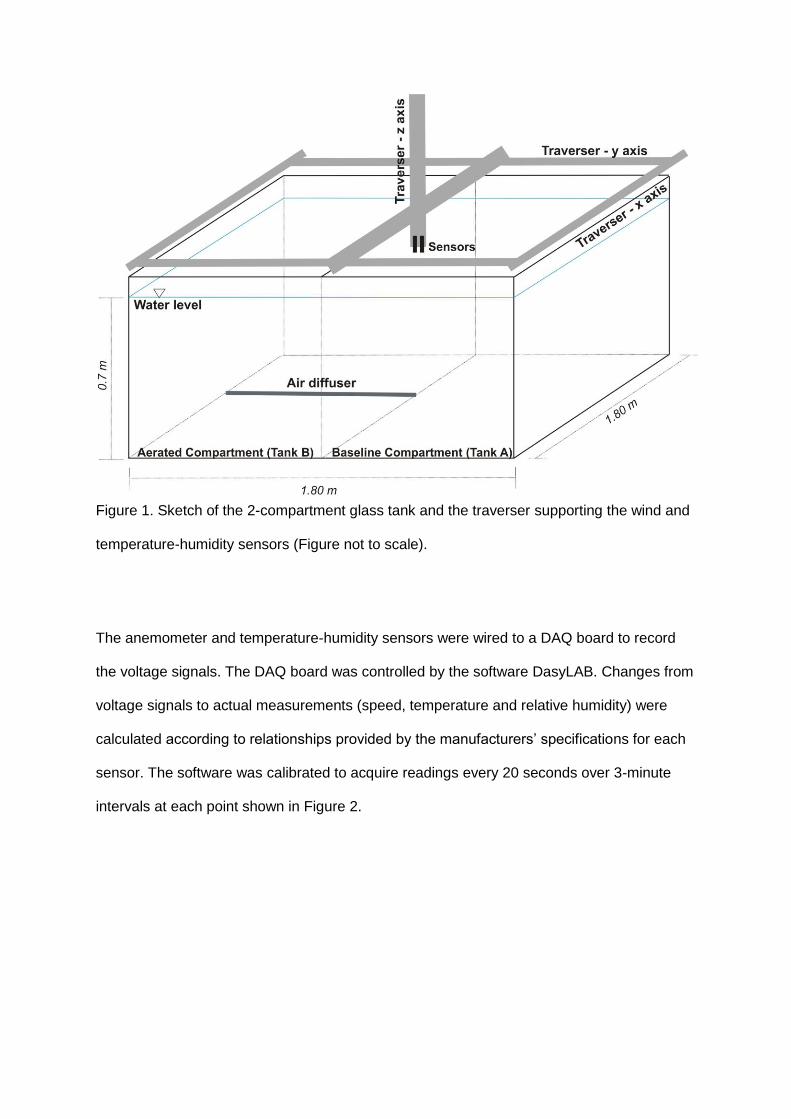
Figure 1. Sketch of the 2-compartment glass tank and the traverser supporting the wind and

temperature-humidity sensors (Figure not to scale).

The anemometer and temperature-humidity sensors were wired to a DAQ board to record

the voltage signals. The DAQ board was controlled by the software DasyLAB. Changes from

voltage signals to actual measurements (speed, temperature and relative humidity) were

calculated according to relationships provided by the manufacturers’ specifications for each

sensor. The software was calibrated to acquire readings every 20 seconds over 3-minute

intervals at each point shown in Figure 2.

a) Top View of Compartments A and B

b) Side View (overwater) of Compartment A

c) Side View (overwater) of Compartment B

Figure 2. Top view of compartments (a) A and B and side views of compartments (b) A and

(c) B showing the monitoring points (black and grey balls) (Figure not to scale).

The aeration system comprised an air compressor, an air line, valves and a 0.85-cm long

bar air stone diffuser that ran the full width of the compartment. The system was installed in

Compartment B, as shown in Figure 2. Five valve settings were possible, generating air-flow

rates as low as 3.8 x 10-2 L s-1 to as high as 19 x 10-2 L s-1 at atmospheric pressure. Table 1

summarises the trials conducted for this study. The first round of trials was run with the air

temperature set at 20oC and the second, with the air temperature set as 22oC, totalling ten

runs in all. The temperature of the room was controlled by an air-conditioning system.

Trial Air-flow rate

(Ls-1

)

Room temperature

(oC)

Trial Air-flow rate

(Ls-1

)

Room temperature

(oC)

R1 – T1 3.8 x 10-2

20 R2 – T1 3.8 x 10-2

22

R1 – T2 7.5 x 10-2

20 R2 – T2 7.5 x 10-2

22

R1 – T3 13.0 x 10-2

20 R2 – T3 13.0 x 10-2

22

R1 – T4 16.0 x 10-2

20 R2 – T4 16.0 x 10-2

22

R1 – T5 19.0 x 10-2

20 R2 – T5 19.0 x 10-2

22

Table 1. Summary of the trials: the first round (R1) was conducted with the air temperature

set at 20oC and the second round (R2), with the temperature set at 22oC.

In order to capture the changes in evaporation, which were expected to be very low due to

the absence of solar radiation inside the room, the duration of each trial was three days.

Each trial was run once only; therefore, repeatability for evaporation was not tested.

However, over a three-day run, the humidity, temperature and wind speed sensors were

able to gather measurements 30 times for each monitoring point shown in Figure 2. To

assure the repeatability, the 30 measurements for humidity, temperature and wind speed at

each location were intercompared during each trial. The variations were negligible.

Additionally, the measurements taken at each location were averaged over a one-day

period, obtaining a total of three averages for each trial. These were intercompared as well,

with the difference being insignificant.

Evaporation was determined by assessing the change in surface elevation of the water

surface in each compartment, which was measured using a calliper gauge. The difference in

water level between the beginning and end of each trial was taken as the measurement of

evaporation.

3. Baseline Evaporation and Evaporation under Aeration Conditions

The baseline evaporation and the evaporation under aeration conditions measured for each

trial are plotted in Figure 3. The baseline evaporation rates during the first and second

rounds of trials (R1 and R2) were fairly constant. In R1, where the average room

temperature was 20oC, evaporation rates were around 0.5 mm day-1. For R2, with average

room temperature equal to 22oC, the baseline evaporation was lower at 0.4 mm day-1. The

evaporation was slightly higher during R1 due to a slightly higher water vapour deficit (ie,

lower relative humidity) above the water surface.

a) R1 – Room Temperature = 20oC b) R2 – Room Temperature = 22

oC

Figure 3. Measured baseline evaporation and evaporation under aeration conditions during

(a) R1 and (b) R2. Error associated with the measurements = ± 0.02 mm day-1.

Under aeration conditions, evaporation rates were found to increase with an increase of air-

flow rate. During R1, the evaporation rate for the lowest air-flow rate (trial R1-T1) was 0.52

mm day-1 and, for the highest (trial R1-T5), 1.17 mm day-1. For R2, evaporation rates for the

lowest and highest air-flow rates were 0.6 mm day-1 and 1.20 mm day-1 respectively. For the

intermediate air-flow rates, the measured evaporation rates were between those two

extremes in both rounds of trials.

Figure 4 graphs the change in evaporation under aeration conditions in relation to the

baseline evaporation for the two rounds.

0.00

0.30

0.60

0.90

1.20

1.50

0.03 0.08 0.13 0.18

Evap

ora

tio

n (

mm

/day)

Air flow rate (L/s)

Baseline Aeration

0.00

0.30

0.60

0.90

1.20

1.50

0.03 0.08 0.13 0.18

Evap

ora

tio

n (

mm

/day)

Air flow rate (L/s)

Baseline Aeration

a) Absolute increase in evaporation b) Percentage increase in evaporation

Figure 4. Increase in evaporation under aeration conditions as compared to baseline

evaporation during R1 and R2. (a) Absolute values; error associated with the measurements

= ± 0.04 mm day-1. (b) Percentage values

The increase in evaporation under aeration conditions as compared to the baseline

evaporation was low for low air-flow rates and higher for high air-flow rates. For R1, the

change in evaporation varied from 0.01 to 0.7 mm day-1, representing relative increases of

1.9% and 135% respectively. For R2, the changes varied from 0.2 to 0.8 mm day-1. In

percentage terms, these changes represent 49% and 200% respectively.

Figure 5 shows the variation in the vapour pressure deficit over the water of the two

compartments for R1 and R2. The deficit was computed as the difference between the

saturated vapour pressure at water temperature and the actual vapour pressure measured

at the uppermost monitoring points, at a height of 65 cm above the water. Because the water

surface temperature did not change significantly over the trials and did not differ between the

baseline compartment and the aerated compartment, the saturated vapour pressure was

nearly constant over each round of experiments. For R1, it was around 22 mbar, and for R2

it was around 25 mbar, with the difference attributed to a slightly higher water temperature

during the second round. Similarly, the actual vapour pressure over the non-aerated water

did not vary significantly among the trials within each round. In R1, the actual vapour

pressure measured at 65 cm above the water was around 18 mbar and, in R2, it was around

0.00

0.25

0.50

0.75

1.00

0.03 0.08 0.13 0.18

Evap

ora

tio

n In

cre

ase

(mm

/da

y)

Air flow rate (L/s)

R1 R2

0%

40%

80%

120%

160%

200%

0.03 0.08 0.13 0.18

Evap

ora

tio

n In

cre

ase

(%)

Air flow rate (L/s) R1 R2

22 mbar. Therefore, the water vapour deficit was nearly constant for the baseline trials,

which can be verified from the dot points in Figure 5.

a) R1 – Room Temperature = 20oC b) R2 – Room Temperature = 22

oC

Figure 5. Baseline water vapour deficit and water vapour deficit under aeration conditions

during (a) R1 and (b) R2 at a height of 65 cm above the water. Approximate error = ± 2.2%.

The water vapour deficit for the trials with the aeration system operating decreased with the

increase in the air-flow rates, indicating there was more moisture over the water when the

aeration system was operating, and that this moisture content increased as the air-flow rates

were increased. For trials R1-T1 and R2-T1 (correspondent to the lowest air-flow rate

tested), the water vapour deficit was close to the baseline deficit. For trials R1-T5 and R1-T5

(the highest air-flow rates), the deficit was much less than the baseline deficit.

Between the two rounds, it can be noted that the deficit of water vapour in the air was higher

during R1 than during R2 for the baseline trials (Figure 5, dot points). This explains the

slightly higher rate of evaporation during R1 shown in Figure 3. For the aerated cases, the

water vapour deficit did not differ by much between the two rounds (Figure 5, squares),

resulting in similar rates of evaporation (Figure 3).

The relative humidity is an indicator of the level of water vapour saturation in the air, and is

graphed in Figure 6. For the air above the water of the non-aerated compartment, the

relative humidity was nearly constant and equal to 75% during R1, and around 81% in R2.

Conversely, for the aerated compartment, the relative humidity was higher for the high air-

1.0

2.0

3.0

4.0

5.0

0.03 0.08 0.13 0.18

Vap

ou

r P

ressu

re G

rad

ien

t (m

ba

r)

Air flow rate (L/s)

Baseline Aeration

1.0

2.0

3.0

4.0

5.0

0.03 0.08 0.13 0.18

Vap

ou

r P

ressu

re G

rad

ien

t (m

bar)

Air flow rate (L/s)

Baseline Aeration

flow rates tested, again indicating the moisture content was increased with increased

aeration, consequently causing a decrease in the vapour deficit.

a) R1 – Room Temperature = 20oC b) R2 – Room Temperature = 22

oC

Figure 6. Baseline relative humidity and relative humidity under aeration conditions during

(a) R1 and (b) R2 at a height of 65 cm above the water. Absolute error associated with

measurements = ± 2.0%.

While the relative humidity was higher during R2 than during R1, this did not significantly

influence the air moisture deficit – shown in Figure 5 for the aerated trials (square points).

This indicates the rate of evaporation cannot be inferred solely from the value of the relative

humidity, or from the value of the actual vapour pressure in the air; the deficit of vapour

pressure in the air is the real controlling factor. This deficit, besides the humidity in the air,

also depends on the humidity near the water, whose value can be taken as the saturation

value for the surface water temperature.

4. The Influence of the Wind

Wind speed influences evaporation by controlling the rate at which the overwater saturated

air is replaced by other air. Over an evaporative surface, the near water air is filled with

water molecules that have just evaporated and broken free, creating a blanket of moisture in

the air which can slow down evaporation. Following this logic, it would be expected that the

aerated water in our experiment would have lower evaporation than the non-aerated water,

70.0

75.0

80.0

85.0

90.0

95.0

100.0

0.03 0.08 0.13 0.18

Rela

tive H

um

idit

y (

%)

Air flow rate (L/s)

Baseline Aeration

70.0

75.0

80.0

85.0

90.0

95.0

100.0

0.03 0.08 0.13 0.18

Rela

tive H

um

idit

y (

%)

Air flow rate (L/s)

Baseline Aeration

due to its higher overwater humidity and hence inability to absorb much more moisture.

Contrary to this expectation, the aerated water actually experienced more evaporation than

the non-aerated water. The explanation for this lies in the fact that a wind current moving

across a water surface can carry away the newly evaporated water molecules, allowing

more water to evaporate into that space. Moreover, a wind current will carry away more

water molecules at higher speeds, driving more evaporation within a shorter period of time.

However, in this laboratory experiment the air inside the controlled room was still; but after

looking closely at the measured wind speed data near where the bubbles were bursting, a

slight air flow was observed, which could have caused the displacement of humidity

upwards. The following graphs in Figure 7 and 8 illustrate the measured air flow above the

aerated and non-aerated waters for three selected trials (R2-baseline, R2-T1 and R2-T3).

a) R2 – Baseline

b) R2 – T1 (Air-flow rate pumped into the water = 3.8 x 10

-2 L/s)

c) R2 – T5 (Air-flow rate pumped into the water = 19 x 10

-2 L/s)

Figure 7. Overwater air flow measured along the aerated and non-aerated compartments of

the tank during the second round of trials. (a) Baseline; (b) R2-T1; (c) R2-T5. The graphs of

Distance along the tank (cm)

Heig

ht

above

wate

r surf

ace (

cm

)

15 50 90 130 165

20

40

60

0

0.1

0.2

0.3

Distance along the tank (cm)

Heig

ht

above

wate

r surf

ace (

cm

)

15 50 90 130 165

20

40

60

0

0.1

0.2

0.3

Distance along the tank (cm)

Heig

ht

above

wate

r surf

ace (

cm

)

15 50 90 130 165

20

40

60

0

0.1

0.2

0.3

Air F

low

(m/s

) A

ir Flo

w (m

/s)

Air F

low

(m/s

)

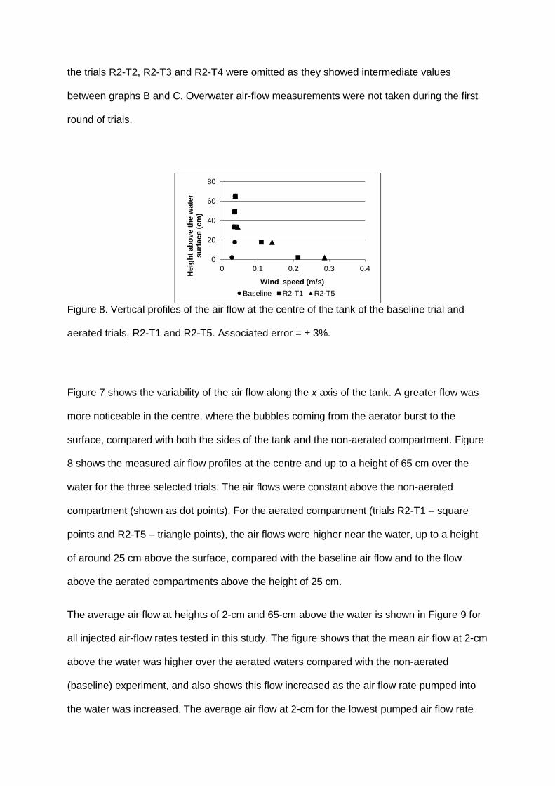
the trials R2-T2, R2-T3 and R2-T4 were omitted as they showed intermediate values

between graphs B and C. Overwater air-flow measurements were not taken during the first

round of trials.

Figure 8. Vertical profiles of the air flow at the centre of the tank of the baseline trial and

aerated trials, R2-T1 and R2-T5. Associated error = ± 3%.

Figure 7 shows the variability of the air flow along the x axis of the tank. A greater flow was

more noticeable in the centre, where the bubbles coming from the aerator burst to the

surface, compared with both the sides of the tank and the non-aerated compartment. Figure

8 shows the measured air flow profiles at the centre and up to a height of 65 cm over the

water for the three selected trials. The air flows were constant above the non-aerated

compartment (shown as dot points). For the aerated compartment (trials R2-T1 – square

points and R2-T5 – triangle points), the air flows were higher near the water, up to a height

of around 25 cm above the surface, compared with the baseline air flow and to the flow

above the aerated compartments above the height of 25 cm.

The average air flow at heights of 2-cm and 65-cm above the water is shown in Figure 9 for

all injected air-flow rates tested in this study. The figure shows that the mean air flow at 2-cm

above the water was higher over the aerated waters compared with the non-aerated

(baseline) experiment, and also shows this flow increased as the air flow rate pumped into

the water was increased. The average air flow at 2-cm for the lowest pumped air flow rate

0

20

40

60

80

0 0.1 0.2 0.3 0.4

Heig

ht

ab

ov

e t

he

wate

r su

rface (

cm

)

Wind speed (m/s)

Baseline R2-T1 R2-T5

was 0.080 m s-1 and, for the highest, it was 0.125 m s-1. The average air flow above the non-

aerated (baseline) water was 0.035 m s-1. At 65-cm, the average air flow above the aerated

water was the same as the baseline air flow, at 0.035 m s-1. The error associated with the

data shown in Figures 8 and 9 is ± 3%. From Figure 7 and 8 it can be seen that the height

up to which the air-bubble bursting process influenced the overwater air was around 25 cm

above the water. Beyond this height, the air flow above the aerated water was basically the

same as the baseline air flow. From Figure 8, it can also be seen that water circulation and

turbulence promoted by air-bubble plumes in water far from the bubble core have negligible

effect on overwater air flow since no or little variation was found at locations away from the

core.

a) 2-cm height b) 65-cm height

Figure 9. Average air flows at 2-cm and 65-cm above the water of the non-aerated and

aerated compartments. Associated error = ± 3%.

The bulk aerodynamic formula for evaporation (Dalton, 1802) is one of the most appropriate

formula to explain the effect of the wind on the overwater humidity and, consequently, on

evaporation. The formula states that evaporation rates from free water surfaces are

proportional to the vapour pressure deficit above the water surface, and that this

proportionality is controlled by the wind speed over the water:

- (1)

0

0.05

0.1

0.15

0.03 0.08 0.13 0.18

Win

d S

pe

ed

(m

/s)

Air flow rate (L/s)

Baseline Aeration

0

0.05

0.1

0.15

0.03 0.08 0.13 0.18

Win

d S

pe

ed

(m

/s)

Air flow rate (L/s)

Baseline Aeration

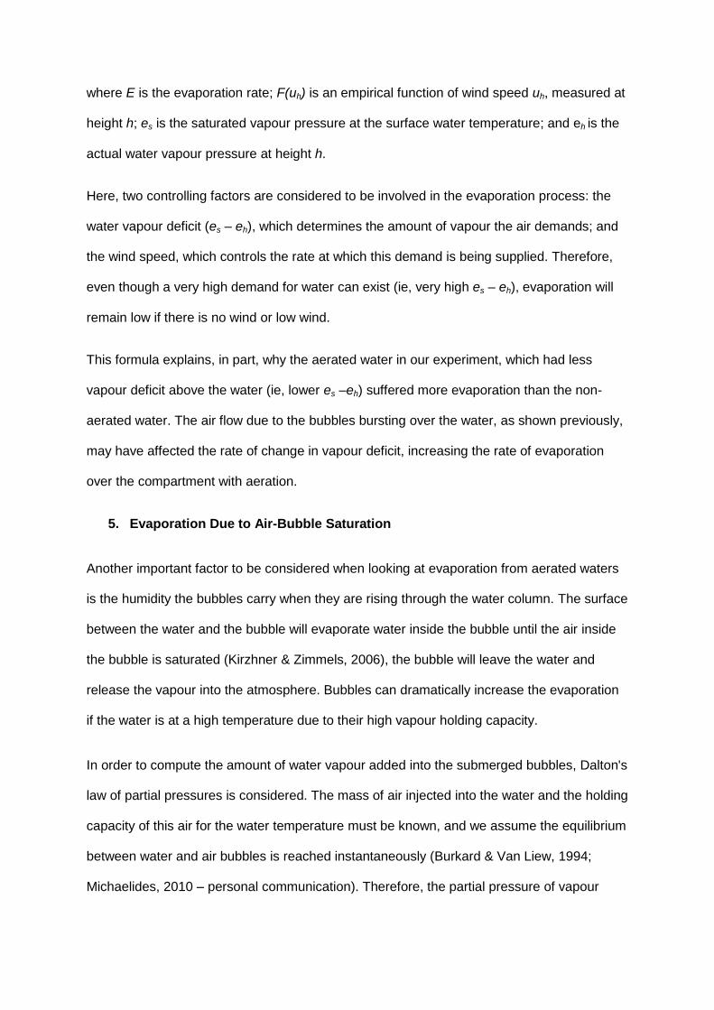
where E is the evaporation rate; F(uh) is an empirical function of wind speed uh, measured at

height h; es is the saturated vapour pressure at the surface water temperature; and eh is the

actual water vapour pressure at height h.

Here, two controlling factors are considered to be involved in the evaporation process: the

water vapour deficit (es – eh), which determines the amount of vapour the air demands; and

the wind speed, which controls the rate at which this demand is being supplied. Therefore,

even though a very high demand for water can exist (ie, very high es – eh), evaporation will

remain low if there is no wind or low wind.

This formula explains, in part, why the aerated water in our experiment, which had less

vapour deficit above the water (ie, lower es –eh) suffered more evaporation than the non-

aerated water. The air flow due to the bubbles bursting over the water, as shown previously,

may have affected the rate of change in vapour deficit, increasing the rate of evaporation

over the compartment with aeration.

5. Evaporation Due to Air-Bubble Saturation

Another important factor to be considered when looking at evaporation from aerated waters

is the humidity the bubbles carry when they are rising through the water column. The surface

between the water and the bubble will evaporate water inside the bubble until the air inside

the bubble is saturated (Kirzhner & Zimmels, 2006), the bubble will leave the water and

release the vapour into the atmosphere. Bubbles can dramatically increase the evaporation

if the water is at a high temperature due to their high vapour holding capacity.

In order to compute the amount of water vapour added into the submerged bubbles, Dalton's

law of partial pressures is considered. The mass of air injected into the water and the holding

capacity of this air for the water temperature must be known, and we assume the equilibrium

between water and air bubbles is reached instantaneously (Burkard & Van Liew, 1994;

Michaelides, 2010 – personal communication). Therefore, the partial pressure of vapour

inside the bubbles must equal the saturation pressure associated with the temperature of the

liquid (Turns, 2000). A reduction in air mass through diffusion could be considered; however,

the bubble-water contact time in aerated lakes is rapid enough to make the diffusion process

negligible (Fuster & Zaleski, 2010). McGinnis et al. (2006) showed that dissolution of gas

would be important only in depths of more than 100 metres.

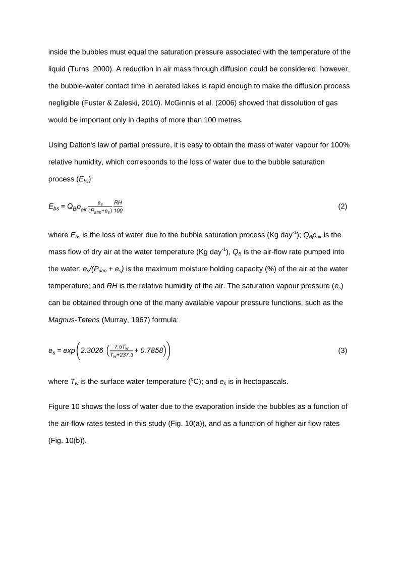
Using Dalton's law of partial pressure, it is easy to obtain the mass of water vapour for 100%

relative humidity, which corresponds to the loss of water due to the bubble saturation

process (Ebs):

(2)

where Ebs is the loss of water due to the bubble saturation process (Kg day-1); QB air is the

mass flow of dry air at the water temperature (Kg day-1), QB is the air-flow rate pumped into

the water; es/(Patm + es) is the maximum moisture holding capacity (%) of the air at the water

temperature; and RH is the relative humidity of the air. The saturation vapour pressure (es)

can be obtained through one of the many available vapour pressure functions, such as the

Magnus-Tetens (Murray, 1967) formula:

(3)

where Tw is the surface water temperature (oC); and es is in hectopascals.

Figure 10 shows the loss of water due to the evaporation inside the bubbles as a function of

the air-flow rates tested in this study (Fig. 10(a)), and as a function of higher air flow rates

(Fig. 10(b)).

a) Range of air-flow rates = 0.04 to 0.20 L/s b) Range of air-flow rates = 0.00 to 400 L/s

Figure 10. Loss of water due to bubble saturation (Ebs) during R1 and R2 (a). The higher

losses during R2 are due to the higher temperature which increases the moisture holding

capacity of the air bubbles. Approximate error = ± 4%. (b) is an extrapolation for air-flow

rates as high as 400 L s-1.

From Figure 10(a) it can be seen that loss of water due to bubble saturation increased with

the air flow rate, and that this loss was greater during R2 due to its higher temperature,

which provides for a higher moisture-holding capacity of the air. It can also be seen from

Figure 10(b) that the water loss for air-flow rates above the range tested in this study follows

an increasing linear trend, with the slope being defined by the water temperature.

Water loss due to bubble saturation was small compared with the total evaporation

measured in this laboratory experiments. The rates shown in Figure 10(a) varied from 2.0%

to 6.0% of the total evaporation measured for the trials. The significance of the bubble

saturation process increased with the increase in the air flow rate - for the lowest air-flow

rate tested (3.8 x 10-2 L s-1), the proportion of water loss attributed to the bubble saturation

process was 2.3% during R1 and R2; and for the highest air-flow rate (19 x 10-2 L s-1), it was

5.0% and 5.8% for R1 and R2 respectively.

The proportion of water loss due to bubble saturation to the total evaporation from an

aerated open water reservoir, however, would be much less than the proportions found from

0.00

0.03

0.06

0.09

0.12

0.15

0.03 0.08 0.13 0.18

Evap

ora

tio

n (

L/d

ay)

Air flow rate (L/s)

R1 R2

0.00

0.05

0.10

0.15

0.20

0.25

0.30

0 100 200 300 400

Evap

ora

tio

n (

m3/d

ay)

Air flow rate (L/s)

R1 R2

this experiment, because the area of the plume within an open water reservoir would be

significantly less than that of the reservoir.

We used North Pine Dam, in Australia, to illustrate this explanation. The reservoir was

aerated at a total rate of 0.33 m3 s-1 (330 L s-1) from 15 October 1995 to 13 December 1995

(Moshfeghi et al., 2005) to break down the thermal stratification in the water column. The

water temperature under aeration conditions was modelled using the model DYRESM

(Imberger & Patterson, 1981). The surface area of the reservoir was 21.36 km2, and the total

baseline evaporation calculated using the Penman-Monteith model (Monteith, 1965) for the

two months was 200 mm. If the proposed methodology to find the loss of water due to the

aeration was applied, the loss of water due to bubble saturation would be 15 m3 for the 2-

month period. If this volume were distributed over the whole surface area of the reservoir,

the height of water reduction would correspond to only 0.001 mm, representing virtually zero

per cent of the total evaporation. However, if the same volume of air was pumped into a

small water body (eg, 2 m2 surface area), the pond would dry up completely in less than 10

days, given the high air-flow rate. Therefore, the proportion of the loss of water due to bubble

saturation in relation to the total evaporation would be significantly large.

6. Empirical Evaporation Estimates

A large number of empirical equations have been developed for predicting evaporation (Sill,

1983) since the late 1800s, when the first empirical investigations were published after

Dalton’s work (Dalton, 1802). Most of these equations are only valid for particular systems

and climates similar to where the measurements were made, meaning their application is

limited (Sartori, 2000). However, given the quantification of evaporation is a difficult task due

to the complex interactions involved in the process, the existing empirical approaches have

been, and continue to be, widely used due to lack of more appropriate theoretical models.

Most of the existing evaporation equations are in the bulk aerodynamic form (Eq. 1) which

states evaporation is proportional to the difference between the vapour pressure near the

surface of the water and the vapour pressure in the air, and that wind velocity affects this

proportionality (Brutsaert, 1982). Despite wide implementation, there is no single universally-

accepted bulk aerodynamic equation due to site-specific conditions that determine different

functions of wind speed.

The wind function F(uh) is usually obtained as an empirical fit to a set of site-specific field

measurements. In its simplest form, uh is plotted against E/(es – eh), with the wind function

obtained from the curve fit (Brutsaert, 1982; Sill, 1983). While many fits are simply a function

in the form of F = a uh , Stelling’s equation (Brutsaert, 1982) has been the preferred function

among evaporation investigators (eg, Fitzgerald, 1886; Rohwer, 1931; Penman, 1948). This

equation has the form F = b + c uh, and allows for evaporation under free convective

condition (ie, when uh = 0), in which case evaporation is driven by the difference in water

vapour concentration between the air close to the water and the surrounding air, rather than

by wind speed. Free convective evaporation may not be as important to open water

reservoirs as it is to enclosed water bodies, such as this laboratory experiment, in which

evaporation is predominantly driven by the gradient of the water vapour above the surface.

In the wind functions, a, b and c are empirical parameters calibrated for each site. Other

investigators have sought to derive improved wind functions by using alternative forms such

as parabolic and power forms (Brady et al., 1969; Jaworski, 1973; Sill, 1983). However,

these different forms do not appear to significantly change the accuracy of the bulk

aerodynamic method, so the simpler forms are still considered adequate for most

applications (Brutsaert, 1982). Other authors (Sartori, 2000; Alvarez, 2007; McJannet et al.,

2011) have taken wind functions developed for specific locations and derived new area-

adjusted functions that can be applied to different-sized water bodies.

Reviews on the wind functions that can be coupled with the bulk aerodynamic formula can

be found in Sweers (1976), Stigter (1980), Sartori (2000), McJannet et al. (2011) and others.

McJannet et al. (2011) emphasised in their paper the limitations of some of the most

traditional wind functions, indicating the range of conditions for which the equations are valid.

Some of the existing and established wind functions are presented in Table 2.

Original source Wind function Units

Carpenter, 1889, 18911

F(u2) = 2.93 + 1.95 u2 mm day-1

kPa-1

Rohwer, 19311

F(u2) = 3.29 + 1.01 u2 mm day-1

kPa-1

Penman, 19481,2

F(u2) = 2.65 + 1.38 u2 mm day-1

kPa-1

Harbeck, 19621,4

F(u2) = 9.17 A-0.05

u2 W m-2

mbar-1

WMO USSR, 19661,2 4

F(u2) = 1.30 + 1.80 u2 mm day-1

kPa-1

WMO USA, 19661,2,4

F(u2) = 1.31 u2 mm day-1

kPa-1

Brutsaert and Yu, 19681 F(u2) = 3.623 A

-0.066 u2 mm day

-1 kPa

-1

Brutsaert and Yu, 19681 - Small pan F(u2) = 2.71 + 2.54 u2 mm day

-1 kPa

-1

Brutsaert and Yu, 19681 - Medium pan F(u2) = 2.31 + 2.11 u2 mm day

-1 kPa

-1

Brutsaert and Yu, 19681 - Large pan F(u2) = 2.46 + 1.71 u2 mm day

-1 kPa

-1

McMillan, 19711 - Fiddlers Ferry model F(u2) = 1.76 + 0.86 u2 mm day

-1 kPa

-1

McMillan, 19711 - Fiddlers Ferry lagoon* F(u2) = 1.16 + 1.07 u2 mm day

-1 kPa

-1

McMillan, 19711 - Fort Colorado F(u2) = 1.59 + 1.06 u2 mm day

-1 kPa

-1

McMillan, 19734,2

(overwater) F(u2) = 3.67 + 2.70 u2 W m-2

mbar-1

McMillan, 19734 (overland) F(u2) = 4.4 + 2.20 u2 W m

-2 mbar

-1

Sweers, 1976

F(u2) = (5 x106 / A)

0.05 (1.29 + 0.95 u2) mm day

-1 kPa

-1

Thom et al., 19813

F(u2) = 1.20 + 1.62 u2 mm day-1

kPa-1

Smith et al., 19941

F(u2) = 2.25 + 1.39 u2 mm day-1

kPa-1

Molina et al. , 20061

F(u2) = 2.06 + 2.28 u2 mm day-1

kPa-1

Rayner, 20073

F(u2) = (1 + 4.1 U2) / (1 + 0.32 u2) mm day-1

kPa-1

Alvarez, 20071

F(u2) = 0.037 log10 A2 – 0.578 log10 A + 3.583 mm day

-1 kPa

-1

McJannet et al., 2011 F(u2) = (2.59 + 1.61 u2 ) A-0.05

mm day-1

kPa-1

1Cited in McJannet et al. (2011);

2Cited in Sartori (2000);

3Cited in Chu et al. (2010);

4Cited in Sweers (1976)

u2 is the wind speed taken at a height of 2 metres in m s-1

; A is the surface area of the water body in m2, W is the

width of the water body in m.

Table 2. Wind functions derived for different sized water bodies and conditions.

Figure 11 shows the plot of the baseline evaporation rates estimated using six of the

functions shown in Table 2 against the observed evaporation rates from the current

laboratory experiment. The functions derived by McMillan (1971; 1973) are widely used, and

valid for a broader range of wind speeds and lake sizes (Sweers, 1976; de Bruin, 1982;

Calder & Neal, 1984; Finch & Hall, 2006). The wind function derived by Thom et al. (1981)

was proven by Chu et al. (2010) to be adequate for wind speeds of less than 3.0 m s-1 (ie, in

conditions where free convective evaporation is relevant). The function of WMO (1966) was

shown by Sweers (1976) to be almost identical to the functions derived by McMillan (1971;

1793) for predictions of evaporation under forced convective conditions.

All functions presented in Figure 11 yielded a reasonable estimate for the free convective

evaporation (ie, wind speed = 0) for the current laboratory data. Their free convective

coefficients (ie, the value of “b” in F = b + c uh) are very close, varying from 1.15 to 1.60 mm

day-1 kPa-1. The observed values of E/(es – eh) from the current experiment yielded b = 1.35

mm day-1 kPa-1, which is represented by the first series of data in Figure 11.

Figure 11. Measured evaporation rates and evaporation rates estimated with six established

wind functions.

7. Evaporation Due to Air-Bubble Bursting Process

In Section 5 it was shown that, under aeration conditions, evaporation is increased by Ebs

(Eq. 2). This loss of water is due to the release of water vapour carried by the saturated

bubbles. In this section, a new component for the estimate of evaporation under aeration

conditions will be derived. This component is related to the additional air speed at the

surface of an evaporative water body due to the bubble bursting process (described in

Section 4), which intuitively will have some effect on the displacement of saturated air above

the surface, thus increasing the rate of local evaporation. This component of the total

evaporation will be referred to as the remaining evaporation (Erem).

0.35

0.40

0.45

0.50

0.55

0.60

0.35 0.40 0.45 0.50 0.55 0.60

Esti

mate

d E

vap

ora

tio

n

(mm

/da

y)

Measured Evaporation (mm/day)

This study

WMO - URSS (1966)

McMillan (1971) - Fort Colorado

McMillan (1973) - overwater

McMillan (1973) - overland

Thom et al. (1981)

Linear (1x1)

The plot of the measured remaining evaporation, after taking away the baseline evaporation

and the evaporation due to the bubble saturation, is graphed in Figure 12 as a function of

the injected air flow rates, showing that the remaining evaporation increases with the

increase in air flow rate. This component of evaporation was higher during the second round

of experiments, with the difference between rounds being attributed to the difference in

temperature – the higher temperature during the second round allowed for higher moisture-

holding capacity of the air near the water. The near-water air (as shown previously in Figures

7 and 8) is affected much more by the ventilation of the bubble burst than is the air far from

the water, which is drier. Therefore, the difference between the two rounds is explained by

the saturation vapour pressure which is, in turn, determined by the water temperature (the

higher the temperature, the higher the saturation vapour pressure). The rate of replacement

of saturated air near the water will be affected by the air flow imparted by the bubble-bursting

process.

Figure 12. The remaining evaporation (Erem) from the aerated compartment after subtracting

the loss of water due to bubble saturation (Ebs) and the free convective evaporation (E) from

the total measured evaporation. Approximate error = ± 0.08 mm day-1.

The effect of the bubble-bursting process on evaporation may be thought of as a function of

the air flow rate released at atmospheric pressure, and bubble core size. Bombardelli et al.

(2007) studied the scaling of aeration bubble plumes in non-stratified water bodies, and

introduced a characteristic length scale D to represent different aeration systems. They

0.00

0.20

0.40

0.60

0.80

1.00

0.03 0.08 0.13 0.18

Evap

ora

tio

n (m

m/d

ay)

Air flow rate (L/s) R1 R2

argued that D could be used to scale vertical, as well as horizontal (radial), distances in

bubble plume systems. The length scale D scales with the bubble slip velocity and the air-

flow rate as follows:

(4)

where g is the gravity; is the entrainment coefficient, us is the bubble slip velocity, taken as

a constant equal to 0.3 m s-1 (Kobus, 1968; Lemckert & Imberger, 1993). The entrainment

coefficient can be taken as a function of the air-flow rate, according to Bernard et al. (2000):

(5)

where h0 is the reference depth (= 10.3 m) and r0 is the radius of the bubble plume, given by

Bernard et al. (2000) as:

(6)

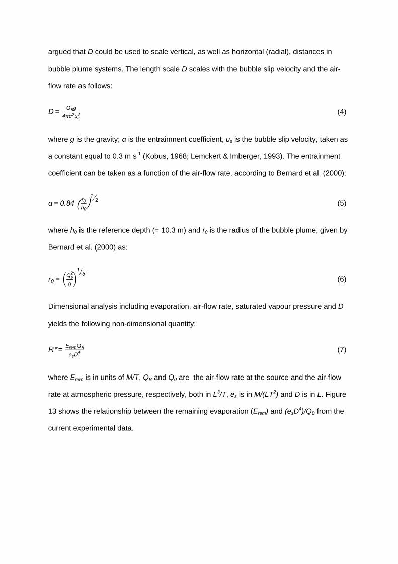
Dimensional analysis including evaporation, air-flow rate, saturated vapour pressure and D

yields the following non-dimensional quantity:

(7)

where Erem is in units of M/T, QB and Q0 are the air-flow rate at the source and the air-flow

rate at atmospheric pressure, respectively, both in L3/T, es is in M/(LT2) and D is in L. Figure

13 shows the relationship between the remaining evaporation (Erem) and (esD4)/QB from the

current experimental data.

Figure 13. The remaining evaporation (Erem) as a function of (esD4)/QB.

From Figure 13, it can be seen that the remaining evaporation can be calculated as a

function of (esD4)/QB using the approximation:

Erem = 4 x 10-5(esD4)/QB (8)

This function will give the remaining evaporation for one air source. The total remaining

evaporation from a given water body may be estimated by multiplying the one-source

evaporation by the number of air sources in operation within the water body.

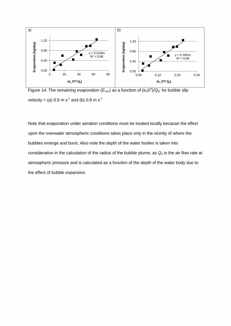
Note the bubble slip velocity has been reported to vary from 0.3 to 0.8 m s-1 under laboratory

conditions (Lima Neto et al., 2008). A different value of the bubble slip velocity would cause

a change in the value of the length scale D, and consequently, in the remaining evaporation.

However, as the slip velocity was taken as a constant, assuming other velocities would only

lead to a different value of the angular coefficient in Eq. 8, Figure 14 shows the relationship

between the laboratory evaporation rates and (esD4)/QB, calculated for bubble slip velocities

= 0.5 and 0.8 m s-1. It is recommended the bubble slip velocity = 0.3 m s-1 be used, and the

relationship represented by Eq. 8 for the calculation of the remaining evaporation from water

bodies. This is reasonable, as in large lakes the bubbles are more likely to reach the terminal

velocity, which is reported to be 0.3 m s-1 on average for bubbles of up to 10 mm in diameter

(Clift et al., 1978).

y = 4E-05x R² = 0.86

0.00

0.40

0.80

1.20

0 10000 20000 30000

Evap

ora

tio

n (

kg

/da

y)

(es D4/ QB)

a) b)

Figure 14. The remaining evaporation (Erem) as a function of (esD4)/QB for bubble slip

velocity = (a) 0.5 m s-1 and (b) 0.8 m s-1

Note that evaporation under aeration conditions must be treated locally because the effect

upon the overwater atmospheric conditions takes place only in the vicinity of where the

bubbles emerge and burst. Also note the depth of the water bodies is taken into

consideration in the calculation of the radius of the bubble plume, as Q0 is the air flow rate at

atmospheric pressure and is calculated as a function of the depth of the water body due to

the effect of bubble expansion.

y = 0.0184x R² = 0.86

0.00

0.40

0.80

1.20

0 20 40 60 80

Evap

ora

tio

n (

kg

/da

y)

(es D4/ Q0)

y = 5.1801x R² = 0.86

0.00

0.40

0.80

1.20

0.00 0.10 0.20 0.30

Evap

ora

tio

n (

kg

/da

y)

(es D4/ Q0)

8. Example of Application – Wivenhoe Dam

This section describes the application of the functions derived for the three components of

evaporation under aeration conditions to an Australian reservoir. These three components -

evaporation due to bubble saturation, background evaporation, and evaporation due to the

bubble-bursting process - were described in Sections 5, 6 and 7 respectively. It is important

to note that Equation 8 was derived from a laboratory experiment and has not been verified

for larger reservoirs. However, since the bubble length scale D, on which evaporation has

been shown to depend, is expected to hold in different conditions of aeration and water

bodies, the results shown in this study are expected to also be valid for real reservoirs.

Wivenhoe Dam is a large dam built on the Brisbane River, with its main purposes being flood

mitigation and the supply of potable water to the south-east Queensland region. At full

capacity this dam has a volume of 1,160 hm3 and a surface area of 107 km2, with a

maximum depth of 40 metres. Wivenhoe is a warm monomictic lake that stratifies from

spring to autumn, with drops of more than 1.5 oC m-1 in the metalimnion. The average

temperature of the hypolimnion is 15.2 oC, varying from 13.8 to 19.3 oC. The annual average

surface temperature is 22.5 oC, varying from 13.8 oC in winter, to 32.6 oC in the summer

(Helfer et al., 2011c).

The theoretical aeration system for this dam was designed using the methodology outlined in

Lemckert et al. (1993). The aeration system comprises 375 sources of air, at an air-flow rate

of 2.0 L s-1 each. The selected period of simulation was three years (from 1 January 1984 to

1 January 1986) due to the availability of reliable meteorological data.

The model DYRESM (Imberger & Patterson, 1981), which has been calibrated and validated

for predictions of evaporation and temperatures for this reservoir (Helfer et al., 2011c), was

used to simulate the water temperature under baseline and aeration conditions. This model

has an algorithm to model the mixing of the water by artificial air-bubble plume systems. The

mixing model is based on the single plume model described by McDougall (1978), which has

been validated with field data in previous studies such as Patterson and Imberger (1989)

and Imteaz and Asaeda (2000).

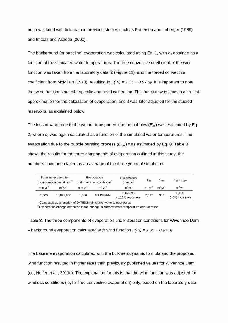
The background (or baseline) evaporation was calculated using Eq. 1, with es obtained as a

function of the simulated water temperatures. The free convective coefficient of the wind

function was taken from the laboratory data fit (Figure 11), and the forced convective

coefficient from McMillan (1973), resulting in F(u2) = 1.35 + 0.97 u2. It is important to note

that wind functions are site-specific and need calibration. This function was chosen as a first

approximation for the calculation of evaporation, and it was later adjusted for the studied

reservoirs, as explained below.

The loss of water due to the vapour transported into the bubbles (Ebs) was estimated by Eq.

2, where es was again calculated as a function of the simulated water temperatures. The

evaporation due to the bubble bursting process (Erem) was estimated by Eq. 8. Table 3

shows the results for the three components of evaporation outlined in this study, the

numbers have been taken as an average of the three years of simulation.

Baseline evaporation

(non-aeration conditions)1

Evaporation

under aeration conditions1

Evaporation

change2

Ebs Erem Ebs + Erem

mm yr-1 m

3 yr

-1 mm yr

-1 m

3 yr

-1 m

3 yr

-1 m

3 yr

-1 m

3 yr

-1 m

3 yr

-1

1,669 58,827,000 1,650 58,159,404 -667,596

(1.13% reduction) 2,097 935

3,032

(~0% increase)

1 Calculated as a function of DYRESM simulated water temperatures.

2 Evaporation change attributed to the change in surface water temperature after aeration.

Table 3. The three components of evaporation under aeration conditions for Wivenhoe Dam

– background evaporation calculated with wind function F(u2) = 1.35 + 0.97 u2

The baseline evaporation calculated with the bulk aerodynamic formula and the proposed

wind function resulted in higher rates than previously published values for Wivenhoe Dam

(eg, Helfer et al., 2011c). The explanation for this is that the wind function was adjusted for

windless conditions (ie, for free convective evaporation) only, based on the laboratory data.

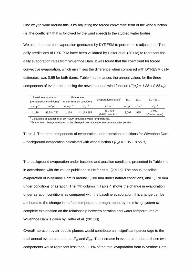
One way to work around this is by adjusting the forced convective term of the wind function

(ie, the coefficient that is followed by the wind speed) to the studied water bodies.

We used the data for evaporation generated by DYRESM to perform this adjustment. The

daily predictions of DYRESM have been validated by Helfer et al. (2011c) to represent the

daily evaporation rates from Wivenhoe Dam. It was found that the coefficient for forced

convective evaporation, which minimises the difference when compared with DYRESM daily

estimates, was 0.65 for both dams. Table 4 summarises the annual values for the three

components of evaporation, using the new proposed wind function (F(u2) = 1.35 + 0.65 u2).

Baseline evaporation

(non-aeration conditions)1

Evaporation

under aeration conditions1 Evaporation change

2 Ebs Erem Ebs + Erem

mm yr-1 m

3 yr

-1 mm yr

-1 m

3 yr

-1 m

3 yr

-1 m

3 yr

-1 m

3 yr

-1 m

3 yr

-1

1,178 41,514,723 1,168 41,163,285 -351,438

(0.8% reduction) 2,097 935

3,032

(~0% increase)

1 Calculated as a function of DYRESM simulated water temperatures.

2 Evaporation change attributed to the change in surface water temperature after aeration.

Table 4. The three components of evaporation under aeration conditions for Wivenhoe Dam

– background evaporation calculated with wind function F(u2) = 1.35 + 0.65 u2

The background evaporation under baseline and aeration conditions presented in Table 4 is

in accordance with the values published in Helfer et al. (2011c). The annual baseline

evaporation of Wivenhoe Dam is around 1,180 mm under natural conditions, and 1,170 mm

under conditions of aeration. The fifth column in Table 4 shows the change in evaporation

under aeration conditions as compared with the baseline evaporation; this change can be

attributed to the change in surface temperature brought about by the mixing system (a

complete explanation on the relationship between aeration and water temperatures of

Wivenhoe Dam is given by Helfer et al. (2011c)).

Overall, aeration by air-bubble plumes would contribute an insignificant percentage to the

total annual evaporation due to Ebs and Erem. The increase in evaporation due to these two

components would represent less than 0.01% of the total evaporation from Wivenhoe Dam

(last column in Table 4). This increase is less than the reduction in evaporation caused by

the aeration system through affecting the water temperature (as shown in Table 4, the

aeration system leads to a reduction in evaporation – very small in magnitude, but still

greater than the losses due to the other two components). The aeration reduces evaporation

by lifting cold bottom water to the surface, thereby reducing the surface temperature. This

reduction, however, only happens in the beginning of the period of artificial destratification

(Helfer et al., 2011c), as after a few days of operation, the water from the bottom of the dam

becomes as warm as the surface temperature. Note that in this study we have simulated

continuous aeration only. However, as presented in Helfer et al. (2011c), intermittent and

continuous aeration are expected to yield similar evaporation reductions as a result of

changes in surface temperature. Intermittent aeration, however, would result in lower losses

of water due to the processes suggested in this study.

9. Conclusions

This paper analysed the effects of aeration by air-bubble plumes on the change in

evaporation from water bodies. A 0.7-m deep tank divided into two compartments and

placed in a windless, temperature-controlled room was used. One of the compartments was

used to measure baseline evaporation, and the other to investigate the effects of different

air-flow rates on evaporation. The air humidity above the water, the temperature of the water

and the ventilation induced by the bubble break-up process at the water surface were all

monitored.

It was found that, compared with baseline evaporation, evaporation from aerated non-

stratified waters increases under aeration conditions, and that this increase is proportional to

the increase in air-flow rates pumped into the water. Moreover, it was found that the increase

in evaporation under aeration conditions may be explained by two processes: one being the

contribution of the “evaporation” inside the bubbles to the losses of water. The other, is the

higher rate of displacement of overwater vapour, at the location where the bubbles emerge

and burst, as a result of the bursting of the bubbles. Two functions were derived from the

laboratory data to predict the water loss due to these two processes. The losses due to the

first process may be estimated as a function of the air flow rate released at the surface and

the saturation vapour pressure at the water temperature, assuming the bubbles reach

equilibrium with the ambient water instantaneously. It was found that the losses due to the

second process could be related to the air-flow rate, the vapour pressure and the length

scale D proposed by Bombardelli et al. (2007) for aeration systems.

Although water losses due to those two processes are significant for small water bodies

such as experimental tanks, if the derived functions are applied to larger temperate water

bodies, these losses become minimal when compared with natural evaporation. Moreover,

the small reduction in evaporation due to the lowering of the water temperature of the

reservoir induced by the mixing process is much higher than the increase in evaporation

from those two processes. The results, therefore, indicate the net effect of aeration by air-

bubble plumes on evaporation from stratified lakes is positive (ie, these systems indeed

reduce evaporation), but the water saving is so small that it does not warrant the use of

these systems for the sole purpose of reducing evaporation.

10. Acknowledgements

Funding for this project was provided by Griffith University Postgraduate Research School

through the GUPRS scholarship; the Australian Government – Department of Innovation,

Industry, Science and Research, through the IPRS scholarship; the Griffith School of

Engineering; and the Urban Water Research Security Alliance.

11. References

ALVAREZ, V. M. 2007. A novel approach for estimating the pan coefficient of irrigation water

reservoirs: application to South Eastern Spain. Agr. Water Manage., 92, pp. 29-40.

BERNARD, R. S., MAIER, R. S. & FALVEY, H. T. 2000. A simple computational model for

bubble plumes. Appl. Math. Model., 24 (3), pp. 215-233.

BOMBARDELLI, F. A. et al. 2007. Modeling and scaling of aeration bubble plumes: a two-

phase flow analysis. J. Hydraul. Res., 45 (5), pp. 617-630.

BRADY, D. K., GRAVES, W. L. & GEYER, J. C. 1969. Surface heat exchange at power

plant cooling lakes. Report 49–5, Dept of Geogr. and Environ. Engng, The Johns Hopkins

University.

BRUTSAERT, W. 1982. Evaporation into the atmosphere, Dordrecht, Reidel. 299 pp.

BRUTSAERT, W. & YU, S. L. 1968. Mass transfer aspects of pan evaporation. J. Appl.

Meteorol., 7 (4), pp. 563-566.

BURKARD, M. E. & VAN LIEW, H. D. 1994. Simulation of exchanges of multiple gases in

bubbles in the body. Resp. Physiol., 95 (2), pp. 131-145.

CALDER, I. R. & NEAL, C. 1984. Evaporation from saline lakes: a combination equation

approach. J. Hydrol. Sci., 29 (1), pp. 89-97.

CARPENTER, K. L. 1889. Section of meteorology and irrigation engineering. Second Annual

Report, Agricultural Experiment Station, State Agricultural College, Fort Collins, Colorado.

CARPENTER, K. L. 1891. Section of meteorology and irrigation engineering. Forth Annual

Report, Agricultural Experiment Station, State Agricultural College, Fort Collins, Colorado.

CHU, C. et al. 2010. A wind tunnel experiment on the evaporation rate of Class A

evaporation pan. J. Hydrol., 381 (3-4), pp. 221-224.

CLIFT, R., GRACE, J. R. & WEBER, M. E. 1978. Bubbles, drops, and particles. New York:

Dover Publications. 400 p.

COOKE, G. D. & CARLSON, R. E. 1989. Reservoir management for water quality and THM

precursor control. Denver: American Water Wiorks Association Research Foundation. 387 p.

DALTON, J. 1802. Experimental essays on the constitution of mixed gases; on the force of

steam or vapour from water and other liquids at different temperatures, both in a Torricellian

vacuum and in air; on evaporation; and on the expansion of gases by heat. Memoirs of the

Literary and Philosophical Society of Manchester, 5-11, pp. 535-602.

DE BRUIN, H. A. R. 1982. Temperature and energy balance of a water reservoir determined

from standard weather data of a land station. J. Hydrol. 59 (3-4), pp. 261-274.

FINCH, J. W. & HALL, R. L. 2006. Evaporation from lakes. In: ANDERSON, M. G. (ed.)

Encyclopedia of Hydrological Sciences. John Wiley & Sons, Ltd.

FITZGERALD, D. 1886. Evaporation. Trans. ASCE, 15, pp. 581-646.

FUSTER, D. & ZALESKI, S. 2010. The importance of liquid evaporation on rectified diffusion

processes. In: 7th Conference on Multiphase Flow, May 30 - June 4, 2010, Tampa, FL.

HARBECK, G. E. J. 1962. A practical field technique for measuring reservoir evaporation

utilizing mass-transfer theory. US Geological Survey Professional Paper 272-E. US

Government Printing Office, Washington, D.C.

HELFER, F., LEMCKERT, C. & ZHANG, H. 2011a. Assessing the effectiveness of air-bubble

plume aeration in reducing evaporation from farm dams in Australia using modelling. In: 6th

International Water Resources Management Conference 2011, May 23-25, 2011, Riverside,

USA. pp. 485-496.

HELFER, F., LEMCKERT, C. & ZHANG, H. 2011b. Investigating techniques to reduce

evaporation from small reservoirs in Australia. In: 34th IAHR World Congress and 33rd

Hydrology & Water Resources Symposium, 26 June - 1 July, 2011, Brisbane, Australia. pp.

1747-1754 (1 cd-rom).

HELFER, F., ZHANG, H. & LEMCKERT, C. 2011c. Modelling of lake mixing induced by air-

bubble plumes and the effects on evaporation. J. Hydrol., 406, pp. 182-198.

IMBERGER, J. & PATTERSON, J. C. 1981. A dynamic reservoir simulation model -

DYRESM. In: FISCHER, H. B. (ed.) Transport Models for Inland and Coastal Waters. New

York: Academic Press. pp. 310-361.

IMBERGER, J. & PATTERSON, J. C. 1990. Physical Limnology. In: WU, T. (ed.) Advances

in Applied Mechanics. New York: Academic Press. pp. 303-475.

IMTEAZ, M. A. & ASAEDA, T. 2000. Artificial mixing of lake water by bubble plume and

effects of bubbling operations on algal bloom. Water Research, 34, pp. 1919-1929.

JAWORSKI, J. 1973. Effects of heated water discharge on the evaporation from a river

surface. J. Hydrol. 19 (2), pp. 145-155.

KIRZHNER, F. & ZIMMELS, Y. 2006. Water vapour and air transport through ponds with

floating aquatic plants. Water Environ. Res., 78 (8), pp. 880-886.

KOBERG, G. E. & FORD, M. E. 1965. Elimination of thermal stratification in reservoirs and

resulting benefits. Geol. Surv. Water Supply Paper 1809-M, Washington DC.

KOBUS, H. E. 1968. Analysis of the flow produced by air bubble systems. In: 11th Coastal

Engineering Conference, 1968, London.

LEMCKERT, C. J. & IMBERGER, J. 1993. Energetic bubble plumes in arbitrary stratification.

J. Hydraul. Eng. ASCE, 119 (6), pp. 680-703.

LEMCKERT, C. J., SCHLADOW, S. G. & IMBERGER, J. 1993. Destratification: some

rational design rules. In: Australian Water and Wastewater Association 15th Federal

Convention, April 18-23, 1993, Gold Coast, Australia.

LIMA NETO, I. E., ZHU, D. Z. & RAJARATNAM, N. 2008. Bubbly jets in stagnant water. Int.

J. Multiphas. Flow, 34, pp. 1130-1141.

LITTLEJOHN, C. L. 2004. Influence of artificial destratification on limnological processes in

Lake Samsonvale (North Pine Dam), Queensland, Australia. MPh Thesis, Griffith University,

Australia.

MCGINNIS, D. F. et al. 2006. Fate of rising methane bubbles in stratified waters: How much

methane reaches the atmosphere? J. Geophys. Res., 111 (C09007).

MCJANNET, D.L. et al. 2008. Evaporation reduction by monolayers: Overview, modelling

and effectiveness. Technical report 6 for the Urban Water Security Research Alliance,

Brisbane, Australia.

MCJANNET, D. L., WEBSTER, I. T. & COOK, F. J. 2011. An evaporation wind function for

open water bodies of variable size. Water Resour. Res. (submitted)

MCMILLAN, W. 1971. Heat dispersal - Lake Trawsfynydd cooling studies. In: Symposium on

freshwater biology and electrical power generation, 1971, Leatherhead, UK. pp. 41-80.

MCMILLAN, W. 1973. Cooling from open water surfaces: final report, Part 1: Lake

Trawsfynydd cooling investigation. Report no. NW/SSD/RR/1204/73 for the Scientific

Services Department, CEGB Machester.

MOLINA, J. M. et al. 2006. A simulation model for predicting hourly pan evaporation from

meteorological data. J. Hydrol., 318 (1-4), pp. 250-261.

MONTEITH, J. L. 1965. Evaporation and the Environment. In: G.E. Fogg (Editor), The state

and movement of water in living organisms. Academic Press, New York, 205-234.

MOSHFEGHI, H., ETEMAD-SHAHIDI, A. & IMBERGER, J. 2005. Modelling of bubble plume

destratification using DYRESM. J. Water Supply, Res. T., 54 (1), pp. 37-46.

MURRAY, F. W. 1967. On the computation of saturation vapor pressure. J. Appl. Meteorol.,

6, pp. 203-204.

PENMAN, H. L. 1948. Natural evaporation from open water, bare soil and grass. In:

Proceedings of the Royal Society. London A193, pp. 120-146.

RAYNER, D. P. 2007. Wind run changes: the dominant factor affecting pan evaporation

trends in Australia. J. Climate, 20, pp. 3379-3394.

ROHWER, C. 1931. Evaporation from free water surfaces. Technical Bulletin 271, US

Department of Agriculture. 96 p.

SARTORI, E. 2000. A critical review on equations employed for the calculation of the

evaporation rate from free water surfaces. Sol. Energy, 68 (1), pp. 77-89.

SILL, B. L. 1983. Free and forced convection effects on evaporation. J. Hydraul. Eng. ASCE,

109 (9), pp. 1216-1231.

SINGLETON, V. L. & LITTLE, J. C. 2006. Designing hypolimnetic aeration and oxygenation

systems - a review. Environ. Sci. Technol., 40 (24), pp. 7512-7520.

SMITH, C. C., LOF, G. & JONES, R. 1994. Measurement and analysis of evaporation from

an inactive outdoor swimming pool. Sol. Energy, 53, pp. 3-7.

STIGTER, C. J. 1980. Assessment of the quality of generalized wind functions in Penman's

equations. J. Hydrol., 45 (3-4), pp. 321-331.

SWEERS, H. E. 1976. A nomograph to estimate the heat-exchange coefficient at the air-

water interface as a function of wind speed and temperature; a critical survey of some

literature. J. Hydrol., 30, pp. 375-401.

THOM, A. S., THONY, J. L. & VAUCLIN, M. 1981. On the proper employment of evaporation

pans and atmometres in estimating potential transpiration. Q. J. Roy. Meteor. Soc., 107, pp.

711-736.

TURNS, S. R. 2000. An introduction to combustion - concepts and applications. Second

edition, McGraw-Hill Publishing Co, London, UK. 565 p.

VAN DIJK, M. & VAN VUUREN, S. J. 2009. Destratification induced by bubble plumes as a

means to reduce evaporation from open impoundments. Water SA (Online), 35 (2), pp. 158-

167.

WMO. 1966. Measurement and estimation of evaporation and evapotranspiration. Technical

Note 83, WMO - Working Group on Evaporation Management. Geneva, Switzerland. 121 p.

WU, R. S. S et al. 2003. Aquatic hypoxia is an endocrine disruptor and impairs fish

reproduction. Environ. Sci. Technol., 37, pp. 1137-1141.

WÜ EST, A., BROOKS, N. H. & IMBODEN, D. M. 1992. Bubble plume modeling for lake

restoration. Water Resour Res, 28 (12), pp. 3235-3250.