inflation, unemployment, and federal reserve policy · lucas and thomas sargent argued that workers...

Chapter 16 (28)

Inflation, Unemployment, and Federal Reserve Policy Chapter Summary Inflation and unemployment are two very important macroeconomic issues. The Phillips curve illustrates the short-run trade-off between the unemployment rate and the inflation rate. The inverse relationship between unemployment and inflation shown by the Phillips curve is consistent with the aggregate demand and aggregate supply (AD-AS) analysis we developed in Chapter 12. The AD-AS model indicates that slow growth in aggregate demand leads to both higher unemployment and lower inflation, and rapid growth in aggregate demand leads to both lower unemployment and higher inflation. This relationship explains why there is a short-run trade-off between unemployment and inflation. In the 1960s, many economists believed that the Phillips curve was a structural relationship that depended on the basic behavior of consumers and firms and that remained unchanged over time. If the Phillips curve was a stable relationship, it would present policymakers with a menu of combinations of unemployment and inflation from which they could choose. Nobel laureate Milton Friedman argued that there is a natural rate of unemployment, which is the unemployment rate that exists when the economy is at potential GDP and to which the economy always returns. As a result, there is no trade-off between unemployment and inflation in the long run, and the long-run Phillips curve is a vertical line at the natural rate of unemployment. There is a short-run trade-off between unemployment and inflation only if the actual inflation rate differs from the inflation rate that workers and firms had expected. During the high and unstable inflation rates of the mid-to-late 1970s, Robert Lucas and Thomas Sargent argued that workers and firms would have rational expectations. Consumers and firms form rational expectations by using all the available information about an economic variable, including the effect of the policy the Federal Reserve is using. Lucas and Sargent argued that if people have rational expectations, expansionary monetary policy will not work. If workers and firms know that an expansionary monetary policy is going to raise the inflation rate, the actual inflation rate will be the same as the expected inflation rate. Therefore, the unemployment rate won’t fall. Many economists remain skeptical of Lucas and Sargent’s argument in its strictest form. Real business cycle models focus on “real” factors—technology shocks—rather than changes in the money supply to explain fluctuations in real GDP. Inflation worsened through the 1970s. Paul Volcker became Fed chairman in 1979, and, under his leadership, the Fed used contractionary monetary policy to reduce inflation. A significant reduction in the inflation rate is called disinflation. This contractionary monetary policy pushed the economy down the short-run Phillips curve. As workers and firms lowered their expectations of future inflation, the short-run Phillips curve shifted down, improving the short-run trade-off between unemployment and inflation. This change in expectations allowed the Fed to switch to an expansionary monetary policy to bring the economy back to the natural rate of unemployment. During Alan Greenspan’s terms as Fed chairman, inflation remained low, and the credibility of the Fed increased. During late 2007 and early 2008, Fed

CHAPTER 16 (28) | Inflation, Unemployment, and Federal Reserve Policy 460

chairman Ben Bernanke was faced with the policy dilemma of dealing with slowing rates of real GDP growth without causing an acceleration in the rate of inflation. Learning Objectives When you finish this chapter, you should be able to: 1. Describe the Phillips curve and the nature of the short-run trade-off between unemployment

and inflation. The Phillips curve illustrates the short-run tradeoff between the unemployment rate and the inflation rate. The Phillips curve’s inverse relationship between unemployment and inflation is consistent with the aggregate demand and aggregate supply analysis developed in Chapter 12. The AD-AS model indicates that slow growth in aggregate demand leads to both higher unemployment and lower inflation, and rapid growth in aggregate demand leads to both lower unemployment and higher inflation. This relationship explains why there is a short-run tradeoff between unemployment and inflation. Many economists initially believed that the Phillips curve was a structural relationship that depended on the basic behavior of consumers and firms and that remained unchanged over time. If the Phillips curve was a stable relationship, then it would present policymakers with a menu of combinations of unemployment and inflation from which they could choose.

2. Explain the relationship between the short-run and long-run Phillips curves. Nobel laureate

Milton Friedman has argued that there is a natural rate of unemployment to which the economy always returns. As a result, there is no tradeoff between unemployment and inflation in the long run, and the long-run Phillips curve is a vertical line at the natural rate of unemployment. There is a short-run tradeoff between unemployment and inflation only if the actual inflation rate turns out to be different from the inflation rate that had been expected by workers and firms. There is a different short-run Phillips curve for every expected inflation rate. Each short-run Phillips curve intersects the long-run Phillips curve at the expected inflation rate. With a vertical long-run Phillips curve, it is not possible to buy a permanently lower unemployment rate at the cost of a permanently higher inflation rate. If the Federal Reserve attempts to keep the economy below the natural rate of unemployment, the inflation rate will increase. Eventually, the expected inflation rate will also increase, which causes the short-run Phillips curve to shift up and pushes the economy back to the natural rate of unemployment. The reverse happens if the Fed attempts to keep the economy above the natural rate of unemployment. In the long run, the Federal Reserve can affect the inflation rate, but not the unemployment rate.

3. Discuss how expectations of the inflation rate affect monetary policy. When the inflation rate is

moderate and stable, workers and firms tend to have adaptive expectations. That is, they form their expectations under the assumption that future inflation rates will be about the same as past inflation rates. During the high and unstable inflation rates of the mid-to-late 1970s, Nobel laureates Robert Lucas and Thomas Sargent argued that workers and firms would have rational expectations. People form rational expectations by using all available information about an economic variable, including the effect of the policy the Federal Reserve is using. Lucas and Sargent argued that if people have rational expectations, expansionary monetary policy will not work. If workers and firms know that an expansionary monetary policy is going to raise the inflation rate, the actual inflation rate will be the same as the expected inflation rate. Therefore, the unemployment rate won’t fall. Many economists remain skeptical of Lucas’ and Sargent’s argument in its strictest form. Real business cycle models focus on “real” factors—technology shocks—rather than changes in the money supply to explain fluctuations in real GDP.


4. Use a Phillips curve graph to show how the Federal Reserve can permanently lower the inflation rate. Inflation worsened through the 1970s. Paul Volcker became Fed chairman in 1979, and under his leadership the Fed used contractionary monetary policy to reduce inflation. This contractionary monetary policy pushed the economy down the short-run Phillips curve. As workers and firms lowered their expectations of future inflation, the short-run Phillips curve shifted down, improving the short-run tradeoff between unemployment and inflation. This change in expectations allowed the Fed to switch to an expansionary monetary policy in order to bring the economy back to full employment at the natural rate. During Alan Greenspan’s term as Fed chairman, inflation remained low and the credibility of the Fed increased. Some economists and policymakers (including Fed chairman Ben Bernanke) believe a central bank’s credibility is increased if it follows a rules strategy for monetary policy, which involves the central bank’s following specific and publicly-announced guidelines for policy. Other economists and policymakers support a discretion strategy for monetary policy, under which the central bank adjusts monetary policy as it sees fit to achieve its policy goals, such as price stability and high employment.

Chapter Review Chapter Opener: Why Does Whirlpool Care About Monetary Policy? (pages 552–553) How does inflation affect monetary policy and how does monetary policy affect inflation? Ben Bernanke, testifying before Congress in March 2007, noted that the Fed was going to continue with a relatively high federal funds rate target because the inflation rate was considered higher than levels consistent with price stability. In 2001, Whirlpool Corporation benefited from the Fed’s expansionary monetary policy that lowered interest rates. Low interest rates encouraged housing demand, which increased the demand for home appliances. The higher interest rates of early 2007, resulting from higher inflation, reduced the demand for home appliances, and Whirlpool’s profits declined.

Helpful Study Hint Read An Inside Look at the end of the chapter for a news article from the Wall Street Journal that discusses new economic research from the Federal Reserve showing that inflation is influenced to a large extent by: 1. The public’s expectation of future inflation. 2. Changes in oil prices. 3. Changes in housing rents. When you start to work full time, you will probably receive annual pay raises. How big a raise should you ask for if it has just been announced that the Fed is going to try to maintain the unemployment rate at 3 percent? The Economics in YOUR Life! at the start of this chapter poses this question. Keep the question in mind as you read the chapter. The authors will answer the question at the end of the chapter.


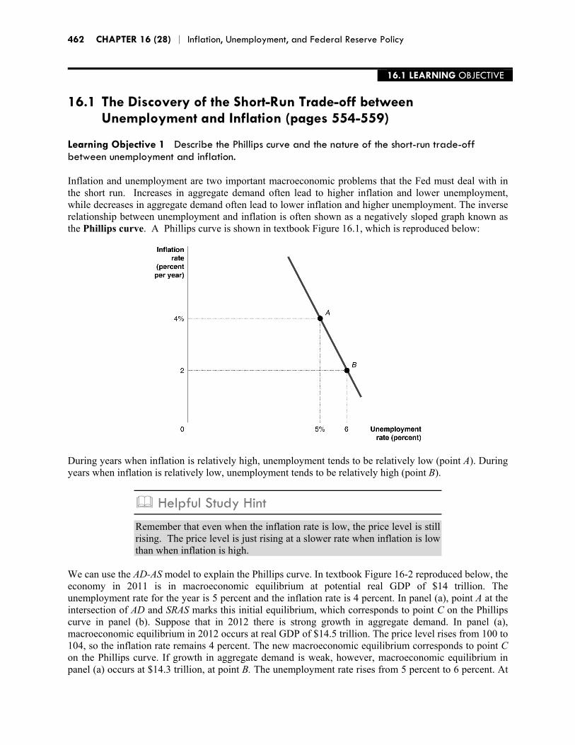
16.1 LEARNING OBJECTIVE 16.1 The Discovery of the Short-Run Trade-off between Unemployment and Inflation (pages 554-559) Learning Objective 1 Describe the Phillips curve and the nature of the short-run trade-off between unemployment and inflation. Inflation and unemployment are two important macroeconomic problems that the Fed must deal with in the short run. Increases in aggregate demand often lead to higher inflation and lower unemployment, while decreases in aggregate demand often lead to lower inflation and higher unemployment. The inverse relationship between unemployment and inflation is often shown as a negatively sloped graph known as the Phillips curve. A Phillips curve is shown in textbook Figure 16.1, which is reproduced below:

During years when inflation is relatively high, unemployment tends to be relatively low (point A). During years when inflation is relatively low, unemployment tends to be relatively high (point B).

Helpful Study Hint Remember that even when the inflation rate is low, the price level is still rising. The price level is just rising at a slower rate when inflation is low than when inflation is high.

We can use the AD-AS model to explain the Phillips curve. In textbook Figure 16-2 reproduced below, the economy in 2011 is in macroeconomic equilibrium at potential real GDP of $14 trillion. The unemployment rate for the year is 5 percent and the inflation rate is 4 percent. In panel (a), point A at the intersection of AD and SRAS marks this initial equilibrium, which corresponds to point C on the Phillips curve in panel (b). Suppose that in 2012 there is strong growth in aggregate demand. In panel (a), macroeconomic equilibrium in 2012 occurs at real GDP of $14.5 trillion. The price level rises from 100 to 104, so the inflation rate remains 4 percent. The new macroeconomic equilibrium corresponds to point C on the Phillips curve. If growth in aggregate demand is weak, however, macroeconomic equilibrium in panel (a) occurs at $14.3 trillion, at point B. The unemployment rate rises from 5 percent to 6 percent. At


the same time, the price level rises only from 100 to 102, so the inflation rate has fallen from 4 percent in the previous year to 2 percent. The short-run equilibrium has moved down the Phillips curve from point C, with an unemployment rate of 5 percent and an inflation rate of 4 percent, to point B, with an unemployment rate of 6 percent and an inflation rate of 2 percent.

A structural relationship depends on the basic behavior of consumers and firms and remains unchanged over long periods. In the 1960s, many economists and policymakers believed the Phillips curve was a structural relationship and represented a permanent trade-off between unemployment and inflation. Today, most economists believe the Phillips curve is not a structural relationship and they view the trade-off between inflation and unemployment as temporary, rather than permanent. A short-run tradeoff exists only because workers and firms sometimes expect the inflation rate to be either higher or lower than it turns out to be. For example, if workers and firms both expect an inflation rate of 5 percent, and the actual inflation rate is 5 percent, wages will rise by 5 percent, so that the real cost of hiring workers will not change (for more on this point, see Short Answer Question 2 in the “Self-Test” section). Because the real cost of hiring workers is the same, the unemployment rate will not change. If, however, workers and firms believe that inflation will be 3 percent, and wages adjust based upon that belief, but actual inflation is 5 percent, then real wages will fall (for more on this point, see Short Answer Question 3 in the “Self-Test” section). Lower real wages will cause firms to hire more workers, and the unemployment rate will decrease. The short-run trade-off between inflation and unemployment comes from unanticipated inflation, not inflation itself. Because there is no trade-off between unemployment and inflation in the long run, economists believe that the long-run Phillips curve is vertical at the natural rate of unemployment. We saw in Chapter 12 that because the LRAS curve is vertical at potential GDP, in the long run, higher prices will not affect the level of real GDP or the level of employment. Similarly, the vertical long-run Phillips curve tells us that higher inflation rates will not lower unemployment in the long run. The level of unemployment that corresponds with potential real GDP is known as the natural rate of unemployment. The long-run Phillips curve is shown below in the graph on the right from textbook Figure 16-3 along with the LRAS curve in the graph on the left.


Helpful Study Hint Remember that at potential real GDP, although there will be no cyclical unemployment there will be frictional and structural unemployment, so the unemployment rate will not be zero.

A long-run vertical Phillips curve indicates that there is no trade-off between inflation and unemployment in the long run. This conclusion is different from the experience of the 1950s and 1960s. There is a trade-off between unemployment and inflation in the short run because workers often expect inflation to be higher or lower than it turns out to be. Differences between the actual inflation rate and the expected inflation rate can cause the unemployment rate to be higher or lower than the natural rate (and real GDP to be higher or lower than potential real GDP). Textbook Table 16-1 reproduced below shows how differences between actual and expected inflation cause differences between actual and expected real wages.


Milton Friedman argued that inflation will increase employment only if inflation is unexpected; that is, if the actual inflation rate is greater than the expected inflation rate. These higher levels of employment are temporary and will disappear when the inaccurate expectations are changed. This short-run trade-off is shown in textbook Table 16-2 below:

Helpful Study Hint Understanding the effects of inflation can be difficult—especially if you’re not an economist. Read Making the Connection: Do Workers Understand Inflation? A higher inflation rate can lead to lower unemployment if both workers and firms mistakenly expect inflation to be lower than it turns out to be. Firms generally have more accurate information about inflation than do workers. Workers often fail to realize that wages will typically rise as prices rise.

16.2 LEARNING OBJECTIVE 16.2 The Short-Run and Long-Run Phillips Curves (pages 559–563) Learning Objective 2 Explain the relationship between the short-run and long-run Phillips curves. The short-run Phillips curve is drawn with the expected rate of inflation held constant. When the expected inflation rate and the actual inflation rate are equal, unemployment will be at the natural rate of unemployment. Textbook Figure 16.4 shows an example of a short-run and a long-run Phillips curve.


In this graph, the short-run and long-run Phillips curves intersect at an inflation rate of 1.5 percent. At the point where the short-run and long-run Phillips curves intersect, we know that the expected inflation rate is equal to the actual inflation rate. Changes in expectations cause shifts in the short-run Phillips curve. Increases in expected inflation cause upward shifts in the short-run Phillips curve, as seen in Figure 16-5 below, which illustrates the impact of the expected inflation rate rising from 1.5 percent to 4.5 percent:

Increases in inflation will cause unemployment to fall, as long as expected inflation does not change. This is a movement along the short-run Phillips curve. When workers and firms begin to adjust their expectations to the actual inflation rate being higher than they had expected, the short-run Phillips curve will shift up to reflect the higher expected inflation rate. Therefore, there is a short-run Phillips curve for


every expected inflation rate. Each short-run Phillips curve intersects the long-run Phillips curve at the expected inflation rate. This is shown in textbook Figure 16-6 below:

Helpful Study Hint The expected inflation rate is held constant along any single short-run Phillips curve. When expected inflation changes, the short-run Phillips curve shifts.

The short-run and long-run Phillips curves have important implications for the conduct of monetary policy. If the Fed tries to use an expansionary monetary policy to lower unemployment by increasing inflation, this can be successful only in the short run. As workers and firms begin to expect higher inflation, the short-run Phillips curve will shift and unemployment will eventually return to the natural rate of unemployment. Thus to keep unemployment below the natural rate of unemployment, the actual inflation rate must constantly increase to stay higher than the upward adjustment of the expected inflation rate. This acceleration of inflation is seen in the following Figure 16-7.


At point C, the current inflation rate will not change because expected inflation equals actual inflation. At point A, the inflation rate will increase because actual inflation is greater than expected inflation and the short-run Phillips curve shifts up. At point B, the inflation rate will decrease because actual inflation is less than expected inflation and the short-run Phillips curve shifts down. The unchanging unemployment rate along the long-run Phillips curve is called the nonaccelerating inflation rate of unemployment (NAIRU).

Helpful Study Hint In the long run, expansionary and contractionary monetary policies will only change the inflation rate. Monetary policy cannot affect the level of real GDP or the unemployment rate in the long run.

The natural rate of unemployment will change over time as a result of changes in demographics, changes in labor market institutions, and the effects of high past levels of unemployment.

Helpful Study Hint Read Making the Connection: Does the Natural Rate of Unemployment Ever Change? At the natural rate of unemployment, only structural and frictional unemployment remain. The amount of frictional and structural unemployment can change over time, however, particularly as demographic changes occur. To give two examples of demographic changes resulting in changes in the natural rate of unemployment: ■ As baby boom workers first hit the labor market in large

numbers during the 1970s and 1980s, because these workers initially had lower job skills, the natural rate of unemployment increased.


■ As the number of young unskilled workers declined in the 1990s, the natural rate fell.

16.3 LEARNING OBJECTIVE

16.3 Expectations of the Inflation Rate and Monetary Policy (pages 564–566) Learning Objective 3 Discuss how expectations of the inflation rate affect monetary policy. How long the economy can remain at a point that is not on the long-run Phillips curve depends on how long it takes workers and firms to adjust their expectations of inflation to the actual inflation rate. People are said to have adaptive expectations if they assume that future rates of inflation will follow the pattern of rates of inflation in the recent past. Experience indicates that how fast workers adjust their expectations depends upon how high the inflation rate is. There are three possibilities:

Low inflation. When inflation is low, workers and firms tend to ignore it. Moderate but stable inflation. With stable inflation, individuals and firms tend to expect

inflation to be what it was last period. This is called adaptive expectations. High and unstable inflation. With higher inflation rates and less stable inflation rates,

workers attempt to estimate inflation rates more accurately. Rational expectations says that workers will use all available information to try to accurately forecast the inflation rate.

Lucas and Sargent argued that if workers and firms have rational expectations and if they expect an expansionary monetary policy will raise the inflation rate, they will use this information in their forecasts of the inflation rate. Consequently, the increase in the inflation rate would not be unanticipated, and the expansionary policy would not cause a decline in unemployment, even in the short run. If Lucas and Sargent are correct, an expansionary policy will cause only a movement along the long-run Phillips curve. This is shown in the following textbook Figure 16-8. In the graph, if workers and firms have adaptive expectations, and expansionary monetary policy will move the economy up the short-run Phillips curve and the unemployment rate will fall. But if workers and firms have rational expectations, the inflation rate will increase, while the unemployment rate will not change.


The logic of Lucas and Sargent’s argument is that the Phillips curve is vertical, even in the short run. With a vertical short-run Phillips curve, expansionary monetary policy cannot reduce the unemployment rate below the natural rate of unemployment. Many economists do not agree that the Phillips curve is vertical in the short run either because they do not believe that workers and firms have rational expectations or because they believe that wages and prices adjust only slowly to changes in aggregate demand. Other economists believe that workers and firms have rational expectations, but argue that fluctuations in unemployment are due to changes in real factors rather than mistakes about the actual inflation rate. These real factors are often referred to as technology shocks, which make it possible to produce more or less output with the same level of employment. Models that focus on real rather than monetary explanations of fluctuations in real GDP and employment are referred to as real business cycle models. Some economists are skeptical of these models because they explain recessions as caused by negative technology shocks, which are uncommon (apart from oil price shocks).

Extra Solved Problem 16-3 Chapter 16 of the textbook includes two Solved Problems. Here is an extra Solved Problem to help you build your skills solving economic problems: Expectation Errors and Unemployment Supports Learning Objective 3: Discuss how expectations of the inflation rate affect monetary policy. Suppose that workers and firms expect that the inflation rate is going to increase from 3 percent to 5 percent. Suppose, though, the inflation rate actually rises only to 4 percent. What would you predict would be the effect on the unemployment rate of the actual inflation rate being less than the expected inflation rate?


SOLVING THE PROBLEM Step 1: Review the chapter material. This problem is about expectations of inflation and monetary policy, so you may want to

review the section “Expectations of the Inflation Rate and Monetary Policy,” which begins on page 564 of the textbook.

Step 2: Use a graph to show the effect of workers and firms expecting the inflation rate to

increase from 3 percent to 5 percent. The increase in the expected inflation rate will shift the short-run Phillips curve upward.

If the inflation rate had increased as workers and firms expected, macroeconomic equilibrium

would move from point A to point B and the unemployment rate would not change. Step 3: Draw a second graph showing the effect of the actual inflation rate being less than

the expected inflation rate. If, however, inflation did not increase as much as workers and firms expected, the real wage

is likely to have increased as nominal wages increased faster than the price level. Higher real wages will result in a higher unemployment rate. So, the new short-run macroeconomic equilibrium will be at point C in the graph, rather than point B. In the short-run macroeconomic equilibrium at point C the inflation rate is lower, but the unemployment rate is higher, than at point B.


16.4 LEARNING OBJECTIVE 16.4 How the Fed Fights Inflation (pages 567–574) Learning Objective 4 Use a Phillips curve graph to show how the Federal Reserve can permanently lower the inflation rate. The high inflation rates of the late 1960s and early 1970s was in part due to the Fed’s attempts to keep the unemployment rate below the natural rate. A supply shock in the 1970s due to higher oil prices made inflation worse. A supply shock will cause the short-run Phillips curve to shift. A supply shock will shift the SRAS to the left. This shift will lower real GDP and increase the price level. On a Phillips curve graph, the Phillips curve will shift up to indicate that both inflation and unemployment have increased. The effect of a supply shock on short-run aggregate supply and the Phillips curve is shown in the following textbook Figure 16-9.


If the Fed uses contractionary monetary policy to fight the inflation resulting from a supply shock, it can lower the inflation rate, but only at the cost of higher unemployment in the short run. If the Fed decides to use expansionary monetary policy to fight the unemployment increases, this will cause more inflation as the economy moves up the short-run Phillips curve. When confronted with this situation in the 1970s, the Fed chose to fight high unemployment with an expansionary monetary policy, even though this decision worsened the inflation rate. Paul Volcker was appointed Fed chairman in August 1979. Under Volcker, the Fed was able to reduce inflation from 10 percent to 5 percent. This disinflation—or significant reduction in the inflation rate—is shown in textbook Figure 16-10 below, where each dot represents the inflation and unemployment rates in a particular year, beginning with 1979:


Alan Greenspan, who followed Volcker as Fed Chairman in 1987, was able to keep the inflation rate low. Greenspan de-emphasized the money supply as a policy target in favor of the federal funds rate. The Federal Open Market Committee has continued to target the federal funds rate in the years since. The fed has also been successful at increasing its credibility by publicly announcing its target for the federal funds rate and by demonstrating a strong commitment to fighting inflation. To increase Fed credibility, some economists have suggested that the Fed follow a rules strategy, where the Fed announces a rule for monetary policy and follows it. Such a rule might be that the money supply should grow at some fixed percentage each year, regardless of economic conditions. Economists who oppose rules support discretionary monetary policy, a policy approach in which the Fed adjusts monetary policy as it sees fit, based on current economic conditions. A middle course is a rule based on economic conditions, such as the Taylor rule, where monetary policy is based on inflation gaps and output gaps. Rules add to the Fed’s credibility by removing flexibility, but rules may not be appropriate in all settings. Some economists suggest that the Fed be more transparent in its inflation goals and announce inflation targets. The Bank of Japan faced credibility problems through the 1990s because the country’s economy experienced falling prices (or deflation). By 1999, the bank lowered its target interest rate (equivalent to the federal funds rate) to zero. Other interest rates remained high as the Japanese public doubted the willingness of the Bank of Japan to continue expansionary monetary policy. The Bank was not willing to state an explicit inflation target, which might have caused workers to increase the rate of inflation they expected and caused the deflation to end.

Extra Solved Problem 16-4 Chapter 16 of the textbook includes two Solved Problems. Here is an extra Solved Problem to help you build your skills solving economic problems: Stagflation and the Short-Run Phillips Curve Learning Objective 4 Use a Phillips curve graph to show how the Federal Reserve can permanently lower the inflation rate. Stagflation is the simultaneous increase in inflation and unemployment. Given the negative slope of the short-run Phillips curve, how is it possible for there to be simultaneous increases in inflation and unemployment? SOLVING THE PROBLEM Step 1: Review the chapter material. This problem is about supply shocks, so you may want to review the section “The Effect of a

Supply Shock on the Phillips Curve,” which begins on page 567 of the textbook. Step 2: Illustrate the short-run trade-off between inflation and unemployment. The short-run Phillips curve shows the short-run trade-off between inflation and

unemployment. Along any short-run Philips curve, an increase in inflation will be accompanied by a decrease in unemployment. The graph illustrates this point by showing that a movement from point A to point B results in lower unemployment and higher inflation.


Step 3: Illustrate the effect of an adverse supply shock. Periods of stagflation are often caused by adverse supply shocks, such as a rapid increase in

oil prices. We saw in Chapter 12 that a supply shock causes the short-run aggregate supply curve (SRAS) to shift to the left. In this chapter, we learned that an adverse supply shock that shifts the SRAS curve to the left will also shift the short-run Phillips curve upward. We show the shift in the short-run Phillips curve caused by a supply shock in the graph below:


Step 4: Analyze the effect of a shift in the short-run Phillips curve. A shift in the short-run Phillips curve creates the possibility of a simultaneous increase in

inflation and unemployment. Stagflation is shown as a movement from point A to point B in the graph above. At point B, both the unemployment rate and the inflation rate are higher than at point A.

Helpful Study Hint Read Don’t Let This Happen to YOU! Don’t Confuse Disinflation with Deflation. Remember disinflation means the inflation rate is falling. As long as the inflation rate is still positive, prices are rising, just not as fast as at the higher inflation rate. Deflation means that the inflation rate is negative and the price level is falling.

Helpful Study Hint Economics in YOUR Life! at the end of the chapter answers the question posed at the start of the chapter: How do you know how much of a raise you can ask for at work if it has just been announced that the Fed is going to try to maintain the unemployment rate at 3 percent? Because the long–run Phillips curve is at about 5 percent, the 3 percent unemployment rate will be below the NAIRU and we would expect the inflation rate to begin to increase. You should ask for a large raise to preserve you future purchasing power.

Key Terms Disinflation. A significant reduction in the inflation rate. Natural rate of unemployment. The normal unemployment rate that exists when the economy is at potential GDP. Nonaccelerating inflation rate of unemployment (NAIRU). The unemployment rate where the inflation rate has no tendency to increase or decrease. Phillips curve. A curve showing the short-run relationship between the unemployment rate and the inflation rate. Rational expectations. Expectations formed by using all available information about an economic variable. Real business cycle models. Models that focus on real rather than monetary explanations of fluctuations in real GDP. Structural relationship. A relationship that depends on the basic behavior of consumers and firms and remains unchanged over long periods.


Self-Test (Answers are provided at the end of the Self-Test.) Multiple-Choice Questions 1. A trade-off between inflation and unemployment exists

a. only in the short run. b. only in the long run. c. in both the short run and the long run. d. in neither the short run nor the long run.

2. When aggregate demand increases, unemployment will usually _________ and inflation will _________. a. rise; rise b. rise; fall c. fall; fall d. fall; rise

3. A Phillips curve is a. a curve showing the relationship between the inflation rate and the money supply. b. a curve showing the short-run relationship between the unemployment rate and the inflation rate. c. a curve showing the relationship between the inflation rate and the exchange rate. d. a curve showing the relationship between the size of the federal budget deficit and the size of the

federal debt.

4. The long-run Phillips curve a. has a negative slope. b. is vertical at the natural rate of unemployment. c. shifts to the right with an increase in inflation. d. shifts to the right as cyclical unemployment decreases.

5. A point near the top left segment of the short-run Phillips curve represents a. a combination of high unemployment and high inflation. b. a combination of high unemployment and low inflation. c. a combination of low unemployment and low inflation. d. a combination of low unemployment and high inflation.

6. Slow growth in aggregate demand leads to a. higher unemployment and higher inflation. b. higher unemployment and lower inflation. c. lower unemployment and lower inflation. d. lower unemployment and higher inflation.


7. Which of the following statements concerning the Phillips curve is correct? a. Most economists in the 1960s and 1970s believed the Phillips curve was vertical in the long run. b. Many economists and policymakers in the 1960s and 1970s viewed the Phillips curve as a

structural relationship. c. Economists have always recognized that there is a permanent trade-off between inflation and

unemployment. d. The only economist who ever viewed the Phillips curve as a structural relationship was A.W.

Phillips.

8. If the long-run aggregate supply curve is vertical, then a. the Phillips curve must be horizontal in the short run. b. the Phillips curve must be vertical in the short run. c. the Phillips curve cannot be downward sloping in the long run. d. the Phillips curve must be downward sloping in the long run.

9. Which of the following statements is correct? a. In the long run, a higher or lower price level has no effect on real GDP. b. In the long run, a higher or lower inflation rate has no effect on the unemployment rate. c. In the long run, the Phillips curve is a vertical line at the natural rate of unemployment. d. all of the above

10. The natural rate of unemployment is a. the prevailing rate of unemployment in the economy in the short run. b. the unemployment rate that results when the economy produces the potential level of real GDP. c. the rate of unemployment when the inflation rate equals zero. d. the lowest unemployment rate on the short-run Phillips curve.

11. According to Milton Friedman, differences between the actual and expected inflation rates could lead the actual unemployment rate to a. rise above or fall below the natural rate. b. rise above the natural rate, but not fall below it. c. fall below the natural rate, but not rise above it. d. remain equal to the natural rate for a long time.

12. If expected inflation is higher than actual inflation, actual real wages in the economy will turn out to be _________ than expected real wages; consequently, firms will hire _________ workers than they had planned. a. higher; more b. higher; fewer c. lower; more d. lower; fewer

13. An increase in expected inflation will

a. shift the short run Phillips curve up. b. shift the long run Phillips curve to the right. c. shift the short run Phillips curve down. d. shift the short run Phillips curve up and the long run Phillips curve to the right.


14. Which change in the inflation rate is more likely to affect the trade-off between inflation and unemployment? a. a change in the inflation rate that is expected b. a change in the inflation rate that is unexpected c. a change in the inflation rate that is exactly equal to the percentage change in the unemployment

rate d. a change in the inflation rate when the unemployment rate equals the natural rate of

unemployment

15. If the annual inflation rate is 3 percent, which of the following will increase real wages? a. an increase in nominal wages of less than 3 percent b. an increase in nominal wages of more than 3 percent c. an increase in nominal wages equal to 3 percent d. a decrease in nominal wages of more than 3 percent

16. If the wage rate is $15.00 and the price level is 125, then the real wage rate is

a. $15.00. b. $12.00. c. $1.20. d. $1.25.

17. If banks need to receive a 4 percent real interest rate on home mortgage loans, what nominal interest rate must they charge if they expect the inflation rate to be 1.5 percent? a. 2.5% b. 5.5% c. 1.5% d. 4%

18. If workers and firms revise their expectations of inflation upward a. there will be a movement downward along the short-run Phillips curve. b. there will be a movement upward along the short-run Phillips curve. c. the short-run Phillips curve will shift up. d. the short-run Phillips curve will shift down.

19. There is a different short-run Phillips curve for every level of the ___________ inflation rate. The inflation rate at which the short-run Phillips curve intersects the long-run Phillips curve equals the ___________ inflation rate. a. actual; expected b. expected; actual c. actual; actual d. expected; expected

20. If the unemployment rate is below the natural rate, the inflation rate tends to ___________ and, eventually, the short-run Phillips curve will shift _______. a. increase; up b. increase; down c. decrease; up d. decrease; down


21. The concept of a nonaccelerating inflation rate of unemployment (NAIRU) helps us to understand why a. in the long run, the Federal Reserve can affect both the inflation rate and the unemployment rate. b. in the long run, the Federal Reserve cannot affect either the inflation rate or the unemployment

rate. c. in the long run, the Federal Reserve can affect the unemployment rate but not the inflation rate. d. in the long run, the Federal Reserve can affect the inflation rate but not the unemployment rate.

22. There are three types of unemployment. Changes in two of the types will cause a change in the natural rate of unemployment. Which two? a. frictional and cyclical unemployment b. structural and cyclical unemployment c. frictional and structural unemployment d. seasonal and cyclical unemployment

23. When do workers and firms tend to ignore inflation? a. when inflation is low b. when inflation is moderate c. when inflation is high d. never

24. If people assume that future rates of inflation will be about the same as past rates of inflation, they are said to have a. naïve expectations. b. adaptive expectations. c. rational expectations. d. consistent expectations.

25. Expectations formed by using all available information about an economic variable are called a. naïve expectations. b. adaptive expectations. c. rational expectations. d. consistent expectations.

26. If workers and firms have rational expectations and wages and prices adjust quickly, an expansionary monetary policy will a. increase the inflation rate, but lower the unemployment rate. b. increase the inflation rate, but not change the unemployment rate. c. increase both the inflation and unemployment rates. d. change neither the inflation nor the unemployment rates.

27. If workers and firms have adaptive expectations or if they ignore inflation, what is the effect of an expansionary monetary policy? a. a move upward along the short-run Phillips curve b. a move downward along the short-run Phillips curve c. a move upward along the long-run Phillips curve d. a move downward along the long-run Phillips curve


28. In a real business cycle model, which of the following best explains an increase in real GDP above the full-employment level? a. adaptive expectations b. an increase in the money supply c. a positive technology shock d. all of the above

29. The monetary explanations of Lucas and Sargent and the real business cycle models are sometimes grouped together under the label of a. monetarism. b. the new classical macroeconomics. c. the new Keynesian macroeconomics. d. the new growth theory.

30. Like the classical economists, the new classical macroeconomists believe that a. the economy cannot correct itself, but requires government intervention in order to remain stable. b. the short-run Phillips curve is horizontal. c. the economy will normally be at its potential level. d. all of the above

31. A supply shock will a. shift the short-run Phillips curve up. b. shift the long-run Phillips curve to the right. c. shift the long-run Phillips curve down. d. shift the short-run Phillips curve up and the long-run Phillips curve to the right.

32. A negative supply shock, such as the OPEC oil price increases of the early 1970s, can be illustrated by a(n) ______________ shift of the short-run aggregate supply curve and a _________________ shift of the short-run Phillips curve. a. leftward; upward b. leftward; downward c. rightward; upward d. rightward; downward

33. How can the Fed fight a combination of rising unemployment and rising inflation? a. By applying expansionary monetary policy, the Fed can solve both problems simultaneously. b. By applying contractionary monetary policy, the Fed can solve both problems simultaneously. c. Not easily. Neither expansionary nor contractionary monetary policy can solve both problems

simultaneously. d. By resorting to the use of fiscal policy instead of monetary policy.

34. In August 1979, President Jimmy Carter appointed Paul Volcker as Chairman of the Board of Governors of the Federal Reserve System. Which of the following statements is true about the state of the economy or the monetary policy chosen by the new Chairman? a. High inflation rates were inflicting significant damage on the economy. b. Paul Volcker chose to reduce the growth rate of the money supply. c. Paul Volcker adopted contractionary monetary policy that caused interest rates to rise and

aggregate demand to decline. d. all of the above


35. After Fed Chairman Paul Volcker decided to fight inflation in 1979, the Fed’s monetary policy resulted in a. lower interest rates. b. a lower unemployment rate. c. lower expectations of future inflation by firms and workers. d. all of the above

36. After Fed Chairman Paul Volcker began fighting inflation in 1979, workers and firms eventually ____________ their expectations of future inflation; consequently, the short-run Phillips curve shifted ___________. a. raised; up b. raised; down c. lowered; up d. lowered; down

37. A significant reduction in the inflation rate is called a. deflation. b. disinflation. c. stagflation. d. cost-push inflation.

38. Paul Volcker’s monetary policy caused the Phillips curve to shift down, but only after several years of high unemployment. This means that, apparently, workers and firms had a. rational expectations, that is, they used all available information to form their expectations of

future inflation. b. adaptive expectations, that is, they changed their expectations of future inflation after the current

inflation rate had fallen. c. naïve expectations, that is, they expected inflation today to be exactly what it was yesterday. d. no expectations at all of future inflation.

39. Disinflation refers to a decline in the _______ _______, while deflation refers to a decline in the _______ _______. a. inflation rate; price level b. price level; inflation rate c. market prices; economy-wide prices d. money supply; price level

40. In order to drive down the inflation rate, the unemployment rate will have to rise more if the short-run Phillips curve is a. flatter. b. steeper. c. vertical. d. upward sloping.

41. During the 1980s and 1990s, the relationship between growth in the money supply and inflation a. broke down, and the Fed announced that it would no longer set targets for M1 and M2. b. strengthened significantly, renewing the Fed’s confidence in using monetary targets for M1 and

M2. c. involved higher inflation rates leading to higher rates of growth of the money supply. d. caused inflation to soar to its highest levels since World War II.


42. A rules strategy refers to a. the central bank’s rules for overseeing the banking system. b. the central bank’s following specific and publicly announced guidelines for policy. c. the Fed’s policy of keeping secret the target for the federal funds rate. d. all of the above

43. A discretion strategy consists of a. adopting the monetarist’s monetary growth rule. b. adjusting monetary policy as the central bank sees fit to achieve its policy goals, such as price

stability and high employment. c. following specific and publicly announced guidelines for policy. d. maintaining a particular monetary policy goal, regardless of the state of the economy.

44. Which of the following is a monetary policy rule where the Fed sets a target for the federal funds rate according to an equation that includes the inflation rate, the equilibrium real federal funds rate, the “inflation gap,” and the “output gap?” a. the growth rule b. the Taylor rule c. the Friedman rule d. the Bernanke rule

45. Which of the following is a problem with deflation? a. Deflation causes real interest rates to fall. b. Deflation causes the value of debts to increase. c. Deflation can cause consumers to consume now rather than postpone purchases. d. all of the above

Short Answer Questions

1. Why does the short-run Phillips curve have a negative slope?

______________________________________________________________________________ ______________________________________________________________________________ ______________________________________________________________________________ ______________________________________________________________________________

______________________________________________________________________________


2. In 2006, average hourly earning in manufacturing was $16.80 and the price level (measured by the GDP deflator) was 116.6. Suppose that in 2007, the inflation rate was 3 percent. How much would average hourly earnings needed to have changed to keep the real wage constant?

______________________________________________________________________________ ______________________________________________________________________________ ______________________________________________________________________________ ______________________________________________________________________________

______________________________________________________________________________

3. Suppose that workers and firms both expect prices to increase by 3 percent. The current average wage rate is $16.80. The price level is 116.6. Show what will happen to the real wage if the actual inflation rate is 5 percent but expected inflation remains at 3 percent. ______________________________________________________________________________ ______________________________________________________________________________ ______________________________________________________________________________ ______________________________________________________________________________

______________________________________________________________________________

4. Why does a vertical long-run aggregate supply curve imply a vertical long-run Phillips curve? ______________________________________________________________________________ ______________________________________________________________________________ ______________________________________________________________________________ ______________________________________________________________________________

______________________________________________________________________________


5. If the Fed tries to reduce the inflation rate using contractionary monetary policy, the impact the policy will have on the unemployment rate depends on how expectations of inflation are formed. Explain. ______________________________________________________________________________ ______________________________________________________________________________ ______________________________________________________________________________ ______________________________________________________________________________

______________________________________________________________________________ 6. Explain the different effects expansionary monetary policy will have on unemployment with

adaptive expectations compared to rational expectations. ______________________________________________________________________________ ______________________________________________________________________________ ______________________________________________________________________________ ______________________________________________________________________________

______________________________________________________________________________ True/False Questions T F 1. A trade-off between inflation and unemployment means that lower unemployment rates

imply higher inflation rates. T F 2. Milton Friedman was the first economist to draw a Phillips curve. T F 3. The short-run Phillips curve has a positive slope. T F 4. The long-run Phillips curve has a negative slope. T F 5. The natural rate of unemployment is zero. T F 6. If nominal wages increase at the same rate as inflation, the real wage will not change. T F 7. If prices rise more than expected, the real wage rate will also rise. T F 8. Unanticipated inflation is the difference between the actual and expected inflation rates. T F 9. An increase in the expected inflation rate will shift the short-run Phillips curve up. T F 10. At points where the short-run Phillips curve crosses the long-run Phillips curve, the

public’s expectations of inflation are accurate. T F 11. In the long run, the Federal Reserve system can affect the inflation rate but not the

unemployment rate. T F 12. The natural rate of unemployment is fixed and does not change. T F 13. If expectations of inflation are rational, then they are based only on past inflation rates. T F 14. A supply shock will shift the SRAS curve to the left and the short-run Phillips curve up. T F 15. Paul Volcker’s contractionary monetary policy reduced inflation without changing the

unemployment rate.


Answers to the Self-Test Multiple-Choice Questions Question Answer Comment 1 a An important consideration for the Fed is that in the short run there can be a

trade-off between unemployment and inflation: Lower unemployment rates can result in higher inflation rates. In the long run, however, this tradeoff disappears and the unemployment rate is independent of the inflation rate.

2 d When aggregate demand increases, unemployment will usually fall and inflation will rise. When aggregate demand decreases, unemployment will usually rise and inflation will fall. As a result, there is a short-run tradeoff between unemployment and inflation.

3 b The Phillips curve is a curve showing the short-run relationship between the unemployment rate and the inflation rate.

4 b The long-run Phillips curve shows the unemployment rate at different inflation rates assuming people’s expectations of inflation are accurate. If expectations are correct, there will be no adjustment in unemployment, and the curve is vertical at the natural rate of unemployment.

5 d Figure 16-1 shows a typical short-run Phillips curve. 6 b The AD-AS model indicates that slow growth in aggregate demand leads to

both higher unemployment and lower inflation. This relationship explains why there is a short-run trade-off between unemployment and inflation, as shown by the downward-sloping Phillips curve.

7 b Because many economists and policymakers in the 1960s and 1970s viewed the Phillips curve as a structural relationship, they believed it represented a permanent trade-off between unemployment and inflation. As long as policymakers were willing to accept a permanently higher inflation rate, they would be able to keep the unemployment rate permanently lower.

8 c Friedman and Phelps noted that economists had come to agree that the long-run aggregate supply curve was vertical. If this was true, then the Phillips curve could not be downward sloping in the long run. There was a critical inconsistency between a vertical long-run aggregate supply curve and a long-run Phillips curve that is downward sloping. Friedman and Phelps argued, in essence, that there is no trade-off between unemployment and inflation in the long run.

9 d In the long run, a higher or lower price level has no effect on real GDP, because real GDP is always at its potential level in the long run. In the same way, in the long run, a higher or lower inflation rate will have no effect on the unemployment rate, because the unemployment rate is always equal to the natural rate in the long run. Figure 16-3 illustrates Friedman’s conclusion that the long-run aggregate supply curve is a vertical line at the potential real GDP and the long-run Phillips curve is a vertical line at the natural rate of unemployment.

10 b At potential real GDP, firms will operate at their normal level of capacity and everyone who wants a job will have one, except the structurally and frictionally unemployed. Milton Friedman defined the natural rate of unemployment as the unemployment rate that exists when the economy is at potential GDP.


11 a Friedman argued that the short-run trade-off between unemployment and inflation exists only because workers and firms sometimes expect the inflation rate to be either higher or lower than it turned out to be. Differences between the expected inflation rate and the actual inflation rate could lead the unemployment rate to rise above or dip below the natural rate.

12 b If expected inflation is higher than actual inflation, actual real wages in the economy will turn out to be higher than expected real wages and firms will hire fewer workers than they had planned.

13 a If the public expects higher inflation, it will be necessary for the inflation rate to rise to keep unemployment at the same level. This is an upward shift in the short-run curve.

14 b Milton Friedman and Edmund Phelps concluded that an increase in the inflation rate increases employment (and decreases unemployment) only if it is unexpected: There is always a temporary trade-off between inflation and unemployment; there is no permanent trade-off. The temporary trade-off comes not from inflation as such, but from unanticipated inflation.

15 b Firms know that only nominal wage increases of more than 3 percent will increase real wages. Workers realize that unless they receive a nominal wage increase of at least 3 percent, their real wage will be falling.

16 b The real wage rate is defined as the nominal wage divided by the price level and multiplied by 100, or ($15.00/125) x 100 = $12.00.

17 b The real interest rate is the nominal interest rate minus the expected inflation rate. If banks need to receive a 4 percent real interest rate on home mortgage loans, they will charge a nominal interest rate of 5.5 percent if they expect the inflation rate to be 1.5 percent.

18 c If workers and firms revise their expectations of inflation upward, the short-run Phillips curve will shift up, which will make the short-run trade-off between unemployment and inflation worse.

19 d There is a different short-run Phillips curve for every expected inflation rate. Each short-run Phillips curve intersects the long-run Phillips curve at the expected inflation rate.

20 a As shown in Figure 16-7, the inflation rate is only stable if the unemployment rate equals the natural rate. If the unemployment rate is below the natural rate, the inflation rate increases and, eventually, the short-run Phillips curve shifts up. If the unemployment rate is above the natural rate, the inflation rate decreases, and, eventually, the short-run Phillips curve shifts down.

21 d As discussed in the chapter, in the long run the economy always returns to the natural rate of unemployment, which is sometimes called the nonaccelerating inflation rate of unemployment, or NAIRU. We can conclude that: In the long run, the Federal Reserve can affect the inflation rate, but not the unemployment rate.

22 c Remember that at the natural rate of unemployment, only frictional and structural unemployment remain. Frictional or structural unemployment can change if there are demographic changes, changes in labor market institutions, or evidence of persistently high past rates of unemployment.

23 a When the inflation rate is low, as it was during most of the 1950s, the early 1960s, the 1990s, and the early 2000s, workers and firms tend to ignore it. For instance, if the inflation rate is low, a restaurant may not want to pay for printing new menus that would show slightly higher prices.

24 b People are said to have adaptive expectations of inflation if they assume that future rates of inflation will be about the same as past rates of inflation.


25 c Expectations formed by using all available information about an economic variable are called rational expectations.

26 b If workers have rational expectations, they will adjust their expectations about inflation following an expansionary monetary policy. As a result, the inflation rate will increase, but the unemployment rate will not change.

27 a If workers and firms ignore inflation, or if they have adaptive expectations, an expansionary monetary policy will cause the short-run equilibrium to move upward along the short-run Phillips curve; inflation will rise and unemployment will fall. If workers and firms have rational expectations, an expansionary monetary policy will cause the short-run equilibrium to move up the long-run Phillips curve. Inflation will still rise, but there will be no change in unemployment.

28 c Real GDP will be above its previous potential level following a positive technology shock and below its previous potential level following a negative technology shock. Real business cycle models focus on real factors, rather than changes in the money supply, to explain fluctuations in real GDP. This is why they are known as real business cycle models.

29 b The approach of Lucas and Sargent and the real business cycle models are sometimes grouped together under the label of new classical macroeconomics, because these approaches share the assumptions that people have rational expectations and that wages and prices adjust rapidly. These assumptions are similar to those held by “classical economists.”

30 c John Maynard Keynes, in his book The General Theory of Employment, Interest, and Money, published in 1936, referred to economists before the Great Depression as “classical economists.” Like the classical economists, the new classical macroeconomists believe that the economy will normally be at its potential level.

31 a A supply shock increases the cost of production. At a given expected inflation rate, increased production costs will reduce real GDP, increasing unemployment, and shifting the short-run Phillips curve up.

32 a As shown in Figure 16-9, when OPEC increased the price of a barrel of oil from less than $3 to more than $10, the SRAS curve shifted to the left. Between 1973 and 1975, real GDP declined from $4,342 billion to $4,311 billion and the price level rose from 31.9 to 38.0. Also, the supply shock shifted the Phillips curve up. In 1973, the U.S. economy had an inflation rate of about 5.5 percent and an unemployment rate of about 5 percent. By 1975, the inflation rate had risen to about 9.5 percent and the unemployment rate to about 8.5 percent.

33 c A combination of rising unemployment and rising inflation places the Federal Reserve in a difficult position. If the Fed uses an expansionary monetary policy to fight the high unemployment rate, the AD curve would shift to the right and the economy’s equilibrium would move up the short-run Phillips curve. Real GDP would increase and the unemployment rate would fall, but at the cost of higher inflation. If the Fed used a contractionary monetary policy to fight the high inflation rate, the AD curve would shift to the left and the economy would move down the short-run Phillips curve. This would cause real GDP to fall and reduce the inflation rate, but at the cost of higher unemployment.


34 d In August 1979, President Jimmy Carter appointed Paul Volcker as Chairman of the Board of Governors of the Federal Reserve System. Along with most economists, Volcker was convinced that high inflation rates were inflicting significant damage on the economy and needed to be reduced. To reduce inflation, he decided to reduce the annual growth rate of the money supply. This contractionary monetary policy raised interest rates, causing a decline in aggregate demand.

35 c As it became clear the Fed was determined to lower the inflation rate, workers and firms lowered their expectations of future inflation.

36 d Fed Chairman Paul Volcker began fighting inflation in 1979 by reducing the growth of the money supply, thereby raising interest rates. By 1982, the unemployment rate had risen to almost 10 percent and the inflation rate had fallen to 6 percent. As workers and firms lowered their expectations of future inflation, the short-run Phillips curve shifted down, improving the short-run trade-off between unemployment and inflation.

37 b Under Paul Volcker’s leadership, the Fed had reduced the inflation rate from more than 10 percent to less than 5 percent. The inflation rate has generally remained below 5 percent ever since. A significant reduction in the inflation rate is called disinflation.

38 b Volcker’s announcement in October 1979 that he planned to use a contractionary monetary policy to bring down the inflation rate was widely publicized. If workers and firms had rational expectations, we might have expected them to quickly reduce their expectations of future inflation. The economy should have moved smoothly down the long-run Phillips curve. However, the economy moved down the existing short-run Phillips curve and only after several years of high unemployment did the Phillips curve shift down. Apparently, workers and firms had adaptive expectations – only changing their expectations of future inflation after the current inflation rate had fallen.

39 a Disinflation refers to a decline in the inflation rate. Deflation refers to a decline in the price level.

40 a How much the unemployment rate would need to rise in order to drive down the inflation rate depends on the steepness of the short-run Phillips curve. The flatter the Phillips curve, the more the unemployment rate will need to rise in order to reduce the inflation rate.

41 a During the 1980s and 1990s, there was a breakdown in the close relationship between growth in the money supply and inflation. Before 1987, the Fed would announce annual targets for how much M1 and M2 would increase during the year. In February 1987, near the end of Paul Volcker’s term, the Fed announced that it would no longer set targets for M1. In July 1993, Alan Greenspan announced that the Fed would also no longer set targets for M2. Instead, the Federal Open Market Committee (FOMC) has relied on setting targets for the federal funds rate to meet its goals of price stability and high employment.

42 b A rules strategy for monetary policy involves the central bank’s following specific and publicly announced guidelines for policy. When the central bank chooses a rule, this strategy requires that it follow the rule, whatever the state of the economy.


43 b Economists and policymakers who oppose the rules strategy support a discretion strategy for monetary policy. With a discretion strategy, the central bank should adjust monetary policy as it sees fit to achieve its policy goals, such as price stability and high employment.

44 b According to the Taylor rule, the Fed should set the target for the federal funds rate according to an equation that includes the inflation rate, the equilibrium real federal funds rate, the “inflation gap,” and the “output gap,” as discussed in Chapter 14.

45 b Deflation can contribute to slow growth by raising real interest rates, increasing the real value of debts, and causing consumers to postpone purchases in the hope of experiencing even lower prices in the future.

Short Answer Responses 1. Increases in inflation, if unanticipated, will cause reductions in real wages. Because wages usually

keep pace with expected inflation, an unexpected increase in inflation will cause the real wage rate to fall. As the real wage rate falls, firms will try to hire more workers to take advantage of the lower cost of resources. This will result in output above potential real GDP and increases in employment, and consequently, a reduction in unemployment. Higher inflation (if unanticipated) will result in lower unemployment, so the short-run Phillips curve has a negative slope.

2. If the nominal wage is $16.80 and the price level is 116.6, then the real wage is: If inflation is 3 percent, the price level will increase to 120.10 (116.6 x 1.03), so to keep the real wage

the same, the new nominal wage will need to increase to $17.30, or Notice that the percentage increase in the wage rate is 3 percent (3.0 = 100 x ($17.30 – $16.80)/

$16.80), which is the same as the inflation rate. 3. If wages rise as much as workers and firms expect prices to rise, wages will also increase 3 percent,

so that wages will rise to $17.30 ($16.80 x 1.03 = $17.30). If prices rise 5 percent, then the new price level will be 122.4 (116.6 x 1.05 = 122.4). The real wage will then be:

Because the real wage in 2006 was $14.41 (see Question 2), the unanticipated inflation reduced the

real wage rate by 2 percent. 4. The vertical long-run aggregate supply curve implies that, regardless of the level of aggregate demand

and the resulting price level, the level of output will in the long-run move toward potential real GDP. Consequently, whatever the inflation rate (the rate of change in the price level), in the long run, output will be at potential real GDP. If output is always at potential real GDP, unemployment will always be at the natural rate of unemployment. Therefore, in the long run at each inflation rate, the

$16.80Real Wage 100 $14.41116.6

= × =

New Wage $17.30$14.41 100 100120.1 120.1

= × = ×

$17.30Real Wage 100 $14.13122.4

= × =


resulting unemployment rate will be the natural rate, which means the long-run Phillips curve will be vertical.

5. If the Fed is successful in using a contractionary monetary policy to reduce inflation, the impact this

will have on the unemployment rate will depend on how expectations are formed. If expectations are formed adaptively, then inflation expectations are based on past inflation. In this case, the lower inflation will cause a movement along a short-run Phillips curve, so that the lower inflation will be accompanied by higher unemployment. This is shown in a movement from point A to point B in the graph below. If expectations of inflation are formed rationally, then because the public is able to predict the reduction in inflation, expected inflation will fall as the inflation rate falls. This implies that the short-run Phillips curve will shift to the left as the inflation rate falls. In this case, the reduction in inflation will not be accompanied by higher unemployment. This is shown in the movement from point A to point C in the graph below.

6. If expectations of inflation are formed adaptively, then an expansionary monetary policy will not be

anticipated by workers or firms, and the inflation caused by the policy will be a surprise. In this case, the higher inflation rate will result in a decrease in the unemployment rate. This is the movement from point A to point B in the graph below. If however, the expansionary monetary policy is anticipated by workers and firms—as would be the case with rational expectations—the resulting inflation will be anticipated and workers and firms will not be surprised by the price increases. In this case, the unemployment rate will not change, and the economy will move from point A to point C as in the following graph.


True/False Answers 1. T 2. F A.W. Phillips drew the graph that indicated the trade-off between inflation and

unemployment. 3. F The short-run Phillips curve has a negative slope, indicating the trade-off between

inflation and unemployment. 4. F The long-run Phillips curve is vertical. 5. F The natural rate of unemployment is the unemployment rate consistent with potential real

GDP. At this point there is no cyclical unemployment, but there will be frictional and structural unemployment.

6. T 7. F If prices rise more than expected, the real wage will fall. 8. T 9. T 10. T 11. T 12. F The natural rate of unemployment may change if there are demographic changes, changes

in labor market institutions, or if the unemployment rate remains high for an extended period.

13. F Rational expectations of inflation are based on all available information about inflation, including expected monetary policy changes.

14. T 15. F During the Volcker time period, as inflation fell, the unemployment rate rose. See Figure

16-10 in the textbook.

inflation, unemployment, and federal reserve policy · lucas and thomas sargent argued that workers...

Documents