inflation targeting in brazil: lessons and challenges · inflation targeting in brazil: lessons and...

106 BIS Papers No 19

Inflation targeting in Brazil: lessons and challenges

André Minella, Paulo Springer de Freitas, Ilan Goldfajn and Marcelo Kfoury Muinhos,1

Central Bank of Brazil

1. Introduction

This paper assesses the inflation targeting regime adopted in July 1999 in Brazil, examining the challenges faced in its first three years. The inflation targeting mechanism has proved to be highly important for macroeconomic stabilisation. In spite of different inflationary pressures, the inflation rate has been maintained at a low level in the context of a floating exchange rate regime and inflationary shocks. We stress three important challenges that are also common in other emerging market economies: construction of credibility, change in relative prices, and exchange rate volatility. Moreover, we describe the methodology used to deal with inflationary shocks, and examine some issues involved in the institutional design of inflation targeting, such as the use of core inflation measures, escape clauses, tolerance intervals, establishment of targets, and target horizon.

We show that the inflation expectations of the private sector have not been departing significantly from the targets even in the face of inflationary shocks. Other evidence also supports the view that the established inflation targets have worked as an important coordinator of expectations. The estimated reaction function of the Central Bank shows that monetary policy has been reacting strongly to inflationary pressures. In particular, the Central Bank reacts to inflation expectations, providing evidence that monetary policy is conducted on a forward-looking basis. We also find some evidence of change in inflation rate dynamics, basically the reduction in the degree of persistence in inflation. The volatility of output and inflation has also decreased in the inflation targeting period.

We also stress the significant inflationary pressures stemming from the change in relative prices in the economy (“administered or monitored” versus “market” prices) and from the exchange rate volatility in the last few years. We estimate the pass-through from exchange rate to inflation rate using a vector autoregression (VAR) estimation, showing the higher pass-through for “administered or monitored” prices.

The Central Bank has developed a methodology to estimate the inflationary effects of change in relative prices, exchange rate depreciation and inflation inertia. The corresponding results help the conduct of monetary policy as it quantifies the sources of inflation.

Section 2 presents an overview of the first three years of inflation targeting. Section 3 assesses the different challenges for the inflation targeting regime. Section 4 presents the methodology used to deal with shocks, and Section 5 examines some issues involved in the institutional design of inflation targeting. A final section concludes the paper.

1 André Minella, Paulo Springer de Freitas and Marcelo Kfoury Muinhos: Research Department, Central Bank of Brazil.

E-mail addresses: [email protected], [email protected], and [email protected]. Ilan Goldfajn: Deputy Governor for Economic Policy, Central Bank of Brazil, and Pontifical Catholic University of Rio de Janeiro (PUC-RJ). E-mail address: [email protected]. The authors would like to thank the participants in the Autumn 2002 Central Bank Economists’ Meeting at the Bank for International Settlements (BIS) and in a seminar at the Central Bank of Brazil for their comments, Richard Clarida for comments in a workshop, and Thaís P Ferreira for her contributions. We are also grateful to Luis A Pelicioni and Marcileide A da Silva for assistance with data. The views expressed are those of the authors and not necessarily those of the Central Bank of Brazil.

BIS Papers No 19 107

2. Overview of the first three years of inflation targeting

The current inflation targeting regime was adopted in mid-1999, after the floating of the currency in January of the same year. In the first two years, inflation rates were kept on target, having absorbed the initial impact of the exchange rate depreciation in 1999. The successful transition was supported by a considerable fiscal improvement, a shift from the primary surplus of 0.01% of GDP in 1998 to 3.23% in 1999, 3.51% in 2000, 3.68% in 2001 and 3.54% in the last 12 months up to August 2002. The macroeconomic policy has three basic elements: floating exchange rate regime, change in the fiscal regime, and inflation targeting.

The targets are established in June year t for calendar year inflation at t + 2, except for 1999 and 2000, when both targets were set in June 1999. The inflation rate is measured by a consumer price index, the IPCA, produced by IBGE. Graph 1 shows the targets for 1999-2004, and actual inflation for 1999-2001. Up to 2002, the tolerance intervals were 2 percentage points above and below the central target, and as of 2003 the intervals were enlarged to 2.5 percentage points. The inflation rate was 8.9% and 6.0% for targets of 8% and 6% for 1999 and 2000, respectively.

Graph 1

Inflation: targets and actual In percentages

8.94

5.97

7.67

0

2

4

6

8

10

12

1999 2000 2001 2002 2003 2004

However, in 2001 and 2002, several external and domestic shocks hit the Brazilian economy with a significant impact on inflation. The inflation rate reached 7.7% in 2001, 1.7 percentage points above the upper limit of the inflation target,2 and is expected to be above the upper limit in 2002 as well. The energy crisis, the deceleration of the world economy, the 11 September attacks on the United States, and the Argentine crisis generated strong pressure for the depreciation of the real in 2001. In October, the average exchange rate had increased by 39.6% (a depreciation of domestic currency of 28.3%) when compared to the average of December 2001. Graph 2 shows the exchange rate level since 1998. In 2002, the shocks included increased risk aversion in capital markets, and uncertainties related to Brazil’s future macroeconomic policies under the upcoming government, leading to a new wave of depreciation.

The change in relative prices in the economy affected the inflation rate significantly as well. The administered-by-contract or monitored prices - administered prices, for short - rose well above the other prices - market prices, for short. The administered prices are defined as the ones little affected by domestic demand and supply conditions or that are in some way regulated by some public agency.

2 The reasons for the non-fulfilment of the target in 2001 were explained in an open letter from the Governor of the Central

Bank of Brazil to the Minister of Finance, available at www.bcb.gov.br.


The group was defined by the Monetary Policy Committee (Copom) in July 2001, and includes oil by-products, fixed telephone, residential electricity, and public transportation. Its weight in the IPCA was 30.8% in June 2002. Furthermore, the energy crisis, from 2001 to the beginning of 2002, and the deregulation of oil by-product markets also led to inflationary pressures.

Graph 2

Real/US dollar exchange rate Monthly averages

1.00

1.50

2.00

2.50

3.00

3.50

Jan

98

Mar

98

May

98

Jul 9

8

Sep

98

Nov

98

Jan

99

Mar

99

May

99

Jul 9

9

Sep

99

Nov

99

Jan

00

Mar

00

May

00

Jul 0

0

Sep

00

Nov

00

Jan

01

Mar

01

May

01

Jul 0

1

Sep

01

Nov

01

Jan

02

Mar

02

May

02

Jul 0

2

Graph 3 shows the exchange rate depreciation, the increase in administered and market prices, and the inflation rate for 2001 and 2002 (up to August). The administered prices rose 10.4% in 2001 and 7.6% in January-August 2002, whereas market prices increased by 6.5% and 3.7%, respectively (the values for 2002 are not annualised).

Graph 3

Exchange rate depreciation and inflationIn percentages

20.9

10.47.7

6.5

24.1

7.64.8 3.7

0

5

10

15

20

25

30

Exchange ratedepreciation

Administered priceinflation

Inflation rate (IPCA) Market price inflation

2001 2002 (up to August)


Graph 4

Contribution to inflation in 2001Percentage of the total and percentage variation

(values within the chart) in the period

Market prices inflation excluding exchange rate pass-through and inertia

28%

Inertia10%

Exchange rate pass-through

38%

Administered prices inflation excluding

exchange rate pass-through and inertia

24%

2.4

1.7

2.9

0.7

Graph 5

Contribution to inflation in 2002 (January-August)Percentage of the total and percentage variation

(values within the chart) in the period

Administered prices inflation excluding

exchange rate pass-through and inertia

13%

Exchange rate pass-through

48%

Inertia17% Market prices inflation

excluding exchange rate pass-through and inertia

22%1.1

0.6

2.3

0.8


Using the structural model of the Central Bank3 and information concerning the mechanisms for the adjustment of administered prices, it is possible to estimate the contribution for the inflation rate stemming from exchange rate pass-through, inflation inertia from the previous year, and inflation of administered prices and market prices that is not explained by the exchange rate pass-through and the inertia referred to. Graphs 4 and 5 show the values for 2001 and January-August 2002. The values in the inner part of the charts are the percentage point contributions for the inflation rate, and, in the outer part, the corresponding proportion. In 2001, 38% of the inflation rate can be explained by the exchange rate depreciation, whereas for January-August 2002 the contribution of the exchange rate reaches 48%.

In 2001 and 2002, the Central Bank acted pre-emptively, aiming at minimising the potential inflationary effects of the different shocks, mainly the exchange rate depreciation and the increase in administered prices. The main guideline of monetary policy was to limit the propagation of the shocks to the other prices in the economy. Graph 6 presents the path of the basic interest rate - the Selic rate - controlled by the Central Bank. Between March and July 2001, the Central Bank raised the interest rate significantly (375 basis points), interrupting the downward trend observed previously. Some improvement in the macroeconomic context at the beginning of 2002 allowed some reduction of the interest rate, interrupted by the inflationary pressure coming from the exchange rate depreciation. If the Central Bank had not acted pre-emptively, inflation would have been higher than actually observed, and the adjustment in the real exchange rate would have taken place in an environment of greater uncertainty. In view of the intensity and magnitude of the shocks that hit the Brazilian economy in 2001 and 2002, the cost in terms of output losses of a policy aimed at offsetting completely these shocks and keeping inflation within the tolerance intervals would have been significantly higher.

Graph 6

Base interest rate (Selic) Monthly averages, in percentages

15.0

20.0

25.0

30.0

35.0

40.0

45.0

Jan

99

Mar

99

May

99

Jul 9

9

Sep

99

Nov

99

Jan

00

Mar

00

May

00

Jul 0

0

Sep

00

Nov

00

Jan

01

Mar

01

May

01

Jul 0

1

Sep

01

Nov

01

Jan

02

Mar

02

May

02

Jul 0

2

We can also verify that there has been a gain in terms of variability of the inflation rate, output and interest rate. Table 1 reports the average, standard error and coefficient of variation (ratio of standard error to average). It compares the first three years of inflation targeting with the Real Plan period before the adoption of inflation targeting. For this last period, the table also reports the figures for a

3 For an overview of the structural model, see Bogdanski et al (2000). Using the aggregate supply curve, which relates the

current inflation of market prices to expected and past headline inflation, output gap and exchange rate change, we estimate the contributions of the exchange rate pass-through and of the inertia from the previous year for market prices. For administered prices, the estimation depends on the criteria used for the price adjustment of specific items.


shorter sample, which excludes the first quarters of the Real Plan, characterised by a transition to stabilisation. The inflation rate is measured by the IPCA, output by seasonally adjusted GDP, and the (nominal) interest rate by the Selic rate. We use quarterly data. In the case of GDP, we use the annualised quarter over quarter growth rates. The variability of output, inflation and the inflation rate is smaller in the inflation targeting period. This does not imply necessarily that there have been gains in terms of trade-off between output and inflation because this result also depends on the magnitude and variability of the shocks that hit the economy. In terms of average, the output growth is higher and the interest rate is lower in the inflation targeting period. The inflation rate is smaller if we compare to the whole period before inflation targeting. In the case of the 1996:01-1999:02 period, the smaller average of the inflation rate is to a large extent a consequence of the pegged exchange rate regime, which turned out to be unsustainable in the medium run.

Table 1

Inflation rate, GDP growth and interest rate Annual average, standard deviation (SD) and coefficient of variation; quarterly data

Inflation rate GDP growth Interest rate

Period Avg SD Coefficient

of variation Avg SD Coefficient of variation Avg SD Coefficient

of variation

Real Plan before inflation targeting:

1994:04-1999:02 10.3 9.2 0.89 2.0 6.3 3.16 35.4 14.1 0.40

1996:01-1999:02 5.8 4.8 0.84 2.0 5.2 2.55 28.2 6.0 0.021

During inflation targeting:

1999:03-2002:02 7.1 3.0 0.42 2.4 3.5 1.46 18.0 1.4 0.08

3. Challenges in inflation targeting

We stress three important challenges in the first three years of inflation targeting in Brazil: construction of credibility, change in relative prices, and exchange rate volatility.

3.1 Constructing credibility

Inflation targeting is, to a large extent, a credibility issue. The Central Bank should act and communicate in a way to convince the market that inflation will be under control. This section shows the estimates of different specifications for Central Bank Taylor-type rules and discusses whether the Central Bank has been effective in controlling inflation expectations. We show that the Central Bank has been reacting strongly to deviations of expected inflation from the target, and that, despite the failure to achieve the target in 2001, inflation expectations remain under control. Furthermore, we present some indications of change in inflation rate dynamics. We conclude that the Central Bank of Brazil has gained credibility in the conduct of monetary policy. The credibility, however, is still under construction as it takes time to achieve it. Besides, the absence of central bank independence in the legal framework is an obstacle to achieving higher levels of credibility.

3.1.1 The reaction function of the Central Bank

We estimate a reaction function of the Central Bank of Brazil that relates the interest rate to expected inflation and to the output gap, allowing also for some interest rate smoothing:

))*()(1( 3120111 jtjttttt Eyii ++−− π−πα+α+αα−+α= (1)


where it is the interest rate, yt is the output gap, jttE +π is inflation expectations and *jt+π is the inflation

target, both referring to some period in the future, as will be explained below.4 The sample consists of monthly data between July 1999, when the regime was formally introduced,5 and June 2002.

We use two different definitions of interest rate. The first one is the base rate (Selic rate) decided by Copom in their meetings. The second definition is the interest rate gap, defined as the difference between the Selic rate and its trend, estimated by an HP filter.6 The motivation to use the gap is to have some idea of how the Central Bank deviates the interest rate from equilibrium when faced by an increase in inflation expectations. This is particularly important for Brazil because, when inflation targeting was introduced, real interest rates were considerably high.7 Therefore, a convergence to steady-state equilibrium would require a downward trend for interest rates. As Bogdanski et al (2001) discuss, in the first two years of the inflation targeting regime, several shocks hit the Brazilian economy and, in many cases, the Copom decision was to leave interest rates constant. This would be equivalent to an increase in interest rates if we consider that the equilibrium interest rate was falling.

Monthly industrial production (seasonally adjusted), as measured by IBGE, is the proxy for output. The output gap was obtained by the difference between the actual and the HP-filtered series.8

We use two sources for inflation expectations. The first is the inflation forecasts of the Central Bank of Brazil presented in the quarterly Inflation Report. The advantage of this source is that Copom should take interest rate decisions based on its own inflation forecasts. The forecasts in the Inflation Report are made assuming a constant interest rate equal to the one decided on in the previous Copom meeting. Therefore, they signal whether the Central Bank should change the interest rate. However, public information about Copom’s inflation forecasts is available only on a quarterly basis. In order to obtain monthly figures, it was necessary to interpolate the data. The second source is obtained by a daily survey that the Central Bank conducts among financial institutions and consulting firms.9 The survey asks what firms expect for year-end inflation in the current and in the following years.10 This expectation, however, is made jointly with an expectation for the interest rate (not necessarily constant).

The Brazilian inflation targeting regime sets year-end inflation targets for the current and the following two years. Since it is necessary to have a single measurement of inflation deviation from the target, it was necessary to create a new variable, weighting the expected deviations from target in different years. The variable chosen was:

)(12

)(12

)12( *11

*++ π−π+π−π

−= ttjttjj EjEjD (2)

where Dt is the measure of expected deviation of inflation from the target, j indexes the month, and t indexes the year. Therefore, Dt is a weighted average of current-year and following-year expected deviation of inflation from the target, where the weights are inversely proportional to the number of months remaining in the year.11 Observe that Dt does not contain inflation expectations referring to two

4 Clarida et al (1998, 2000) estimate forward-looking reaction functions for France, Germany, Italy, Japan, the United Kingdom

and the United States. Instead of using central bank or survey expectations, they employ a Generalised Method of Moments (GMM) estimation. It is basically a forward-looking version of the backward-looking reaction function proposed by Taylor (1993).

5 Decree 3088 of 21 June 1999 established inflation targeting in Brazil. Therefore, the July Copom meeting of that year was the first one under a formal inflation targeting regime.

6 The Hodrick-Prescott filter was passed over the monthly data series between September 1994 (two months after the introduction of the real) and June 2002.

7 During the pegged exchange rate regime, which ended in January 1999, the Selic rate needed to be at high levels in order to prevent a large outflow of reserves. In the first months following the flotation of the real, the Selic rate needed to be kept at high levels to prevent an inflation-exchange rate depreciation spiral.

8 Estimations using output growth and the output gap obtained by extraction of a linear trend were also performed. The results were similar and are not reported in this paper.

9 This survey is available on the Central Bank of Brazil website (www.bcb.gov.br). In this estimation, we use the inflation expectations collected on the eve of Copom meetings, avoiding possible endogeneity problems.

10 In November 2001 the survey started collecting expectations for the following 12 months as well. 11 It is not necessary to have a single measure of inflation deviation. If there were enough data, it would be possible to use

expected inflation for the current and the following years (and possibly more years ahead) in the reaction function. But it


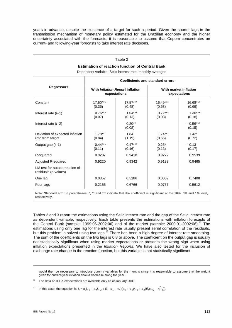
years in advance, despite the existence of a target for such a period. Given the shorter lags in the transmission mechanism of monetary policy estimated for the Brazilian economy and the higher uncertainty associated with the forecasts, it is reasonable to assume that Copom concentrates on current- and following-year forecasts to take interest rate decisions.

Table 2

Estimation of reaction function of Central Bank Dependent variable: Selic interest rate; monthly averages

Coefficients and standard errors

Regressors With Inflation Report inflation

expectations With market inflation

expectations

Constant 17.50***

(0.36) 17.57*** (0.48)

16.49*** (0.63)

16.68*** (0.69)

Interest rate (t−1) 0.76*** (0.07)

1.04*** (0.13)

0.72*** (0.08)

1.36*** (0.18)

Interest rate (t−2) −0.20** (0.08)

−0.56*** (0.15)

Deviation of expected inflation rate from target

1.78** (0.84)

1.84 (1.19)

1.74** (0.66)

1.42* (0.72)

Output gap (t−1) −0.44*** (0.11)

−0.47*** (0.16)

−0.25* (0.13)

−0.13 (0.17)

R-squared 0.9287 0.9418 0.9272 0.9539

Adjusted R-squared 0.9220 0.9342 0.9188 0.9465

LM test for autocorrelation of residuals (p-values)

One lag 0.0357 0.5186 0.0059 0.7408

Four lags 0.2165 0.6766 0.0757 0.5612

Note: Standard error in parentheses; *, ** and *** indicate that the coefficient is significant at the 10%, 5% and 1% level, respectively.

Tables 2 and 3 report the estimations using the Selic interest rate and the gap of the Selic interest rate as dependent variable, respectively. Each table presents the estimations with inflation forecasts of the Central Bank (sample: 1999:06-2002:06) and of the market (sample: 2000:01-2002:06).12 The estimations using only one lag for the interest rate usually present serial correlation of the residuals, but this problem is solved using two lags.13 There has been a high degree of interest rate smoothing. The sum of the coefficients on the two lags is 0.8 or above. The coefficient on the output gap is usually not statistically significant when using market expectations or presents the wrong sign when using inflation expectations presented in the Inflation Reports. We have also tested for the inclusion of exchange rate change in the reaction function, but this variable is not statistically significant.

would then be necessary to introduce dummy variables for the months since it is reasonable to assume that the weight given for current-year inflation should decrease along the year.

12 The data on IPCA expectations are available only as of January 2000.

13 In this case, the equation is )).*()(1( 3120412411 jtjtttttt Eyiii ++−−− π−πα+α+αα−α−+α+α=


Table 3

Estimation of reaction function of Central Bank Dependent variable: gap of Selic interest rate; monthly averages

Coefficients and standard errors

Regressors With Inflation Report inflation expectations

With market inflation expectations

Constant −1.51*** (0.36)

−1.28*** (0.36)

−3.28*** (0.54)

−3.53*** (0.65)

Gap of interest rate (t−1) 0.81*** (0.06)

1.08*** (0.09)

0.71*** (0.08)

1.34*** (0.19)

Gap of interest rate (t−2) −0.25*** (0.06)

−0.54*** (0.15)

Deviation of expected inflation rate from target

5.01*** (0.92)

4.25*** (0.77)

3.70*** (0.58)

3.63*** (0.68)

Output gap (t−1) −0.38** (0.15)

−0.43*** (0.13)

−0.05 (0.13)

0.08 (0.17)

R-squared 0.9653 0.9768 0.9694 0.9797


LM Test for autocorrelation of residuals (p-values)

One lag 0.1254 0.4020 0.0080 0.4255

Four lags 0.0796 0.4754 0.0461 0.4356


Most importantly, the coefficient on inflation expectations is greater than one and significantly different from zero. Employing the Inflation Report’s expectations, the coefficient is 1.8414 and 4.25 using the Selic rate and the gap of Selic, respectively. Therefore, we can conclude that the Central Bank has been reacting strongly to expected inflation. It conducts monetary policy on a forward-looking basis, and responds to inflationary pressures.

It is interesting to note that such coefficients are around 1.4-1.8 when the dependent variable is the Selic rate,15 and above 3.6 when the dependent variable is the gap of the Selic rate. This result supports the view that, given a downward trend for interest rates, Copom decisions to leave the interest rate constant may be interpreted as a tightening of monetary policy. Moreover, in the case of the gap of the Selic rate, the coefficients are significantly different from one in all specifications.

3.1.2 Inflation expectations and the role of targets

A naive analysis of the inflation targeting regime in Brazil might say that this regime has not been successful in controlling inflation. As Graph 7 shows, since mid-2001, 12-month inflation has been above the upper limit of the tolerance interval.16 Nevertheless, inflation outcomes are not a sufficient

14 In this case, the p-value is 0.13, but we have to consider the small size of the sample. 15 Favero and Giavazzi (2002) also estimated a similar reaction function using market expectations, and obtained similar

results (coefficient equal to 1.78). Silva and Portugal (2002) used a different specification, and obtained different results. 16 There are established targets only for year-end inflation. Therefore it was necessary to impute a target to the other months

of the year, which was done by linear interpolation.


statistic for evaluating the performance of the Central Bank. The evolution of inflation expectations, and the role of the target should be more relevant variables for assessing the credibility of the Central Bank. Furthermore, it is necessary to take into account the shocks that hit the economy.

Graph 7

Inflation: targets and actual In percentages

0.0

2.0

4.0

6.0

8.0

10.0

12.0

Jun

99

Aug

99

Oct

99

Dec

99

Feb

00

Apr

00

Jun

00

Aug

00

Oct

00

Dec

00

Feb

01

Apr

01

Jun

01

Aug

01

Oct

01

Dec

01

Feb

02

Apr

02

Jun

02

Central target Upper limitLower limit 12-month inflation rate

Since the introduction of the inflation targeting regime in Brazil, the economy has been hit by inflationary shocks, notably by supply and cost-push shocks. As of 2001, shocks such as the energy crisis, the readjustments of administered prices and the exchange rate depreciation have forced the Central Bank to reassess the trade-off between inflation and output variability. Since then and, in a more systematic way, since January 2002, the conduct of monetary policy has been based on accommodating the first-round effects of supply and cost-push shocks. This means monetary policy will allow relative price movements to affect inflation, but will neutralise the second-round effects.

As long as the market understands the objectives of the Central Bank, and its conduct is credible, inflation expectations should be contained and, except for unforeseen new inflationary shocks, inflation should gravitate around the target. Two conditions are necessary to guarantee that inflation expectations will remain controlled. The first one is clear communication with the market. The market needs to understand why actual inflation was above the target and how monetary policy is being conducted in order to make inflation return to the target. The Central Bank of Brazil communicates with the market via informal speeches or formal documents, such as the minutes of the Copom meetings, which are released one week after the meetings, and the Inflation Report, which is published on a quarterly basis. The second condition for controlling expectations is that the conduct of monetary policy should be consistent with the main guidelines expressed by Copom. In this sense, the reaction function estimated in the previous subsection shows that the Central Bank has been acting consistently with the inflation targeting framework.

Graph 8 suggests that the two conditions stated above have been met. It shows the 12-month ahead inflation that is expected by the market, the 12-month ahead target, and actual 12-month accumulated inflation. We estimate the 12-month ahead expected inflation rate using the inflation expected up to the end of the current year and, for the remaining months necessary to achieve 12 months, the corresponding proportion of following-year expected inflation. The 12-month ahead target is estimated by interpolation. It is clear that inflation expectations have always been below the upper limit of the tolerance interval. This has been true even since the second half of 2001, when actual inflation surpassed the tolerance interval. The correlation coefficient between the actual and expected inflation series is low (0.12). However, there are subsamples where the correlation coefficient is higher. For example, after February 2001, the correlation between the series is 0.70. Even for such subsamples, where inflation expectations tend to move closer to previous inflation, the movements of expectations


tend to be smoother than the movements of actual inflation. As the graph shows, the gap between actual and expected inflation increased after mid-2001, when actual inflation surpassed the upper limit of the tolerance interval. Therefore, especially for this period, the credibility of the Central Bank seemed to be essential to keep inflation expectations under control.

Graph 8

Inflation: 12-month ahead expected inflation, the inflation target and actual inflation

In percentages

0.01.02.03.04.05.06.07.08.09.0

10.0

Jan

00

Mar

00

May

00

Jul 0

0

Sep

00

Nov

00

Jan

01

Mar

01

May

01

Jul 0

1

Sep

01

Nov

01

Jan

02

Mar

02

May

02

Central target Upper limitLower limit Inflation expectationsPrevious 12-month inflation

Other evidence to suggest the gains in credibility of the Central Bank is to evaluate the role of the target in forming expectations. We have run ordinary least squares (OLS) regressions of 12-month ahead market inflation expectations on its own lags, the 12-month ahead inflation target and the interest rate (sample: 2000:01-2002:06). Table 4 reports the results. Since we find serial correlation of residuals with one lag for expected inflation, we also estimate the model using two lags. All coefficients are statistically significant and have the expected sign. The positive coefficient on the interest rate may be explained by the reaction of interest rates to inflationary pressures. When the Central Bank (and the market) foresees higher inflation, the rate of interest is increased. Most importantly, expected inflation reacts significantly to the inflation targets (coefficient equal to 0.96). Since this result could be a consequence of some correlation between targets and past inflation, we also include the actual 12-month inflation rate in the regression (specifications III and IV). This variable is not statistically significant. Therefore, there are indications that the expectations are forward-looking, and the inflation targets play an important role.

In summary, although the actual inflation rate has been above the upper limit of the tolerance interval in 2001 and 2002, the inflation targeting regime has been successful in anchoring expectations. This is a consequence of the gains of credibility that the Central Bank has achieved since the implementation of the inflation targeting regime.


Table 4

Estimation of reaction function of inflation expectations Dependent variable: market inflation rate expectations (adjusted)

Coefficients and standard errors Regressors

I II III IV

Constant −4.23*** (1.30)

−4.75*** (1.31)

−4.22*** (1.32)

−4.92*** (1.35)

Market inflation rate expectations (t−1)

0.24 (0.18)

0.48** (0.19)

0.27 (0.18)

0.50** (0.19)

Market inflation rate expectations (t−2)

−0.39** (0.15)

−0.40** (0.15)

Interest rate (t−1) 0.27*** (0.07)

0.29*** (0.07)

0.25*** (0.08)

0.27*** (0.08)

Inflation rate target (12-month ahead)

0.74*** (0.22)

0.96*** (0.24)

0.70*** (0.23)

0.95*** (0.24)

12-month inflation rate (t−1) 0.06 (0.10)

0.08 (0.11)

R-squared 0.8978 0.9030 0.8993 0.9053



One lag 0.0663 0.5196 0.0652 0.7730

Four lags 0.0160 0.1333 0.0149 0.1316


3.1.3 Change in inflation dynamics

As the inflation targeting regime is supposed to affect the formation of inflation expectations, we can consider the possibility that the backward-looking component in price adjustment has become less important. The share of backward-looking firms could have become smaller and/or firms could give less consideration to past inflation when adjusting prices. This would reduce the degree of persistence in inflation. Following Kuttner and Posen (1999), we estimate a simple aggregate supply curve for the low-inflation period to assess whether the inflation targeting regime was accompanied by some structural change.17 Using monthly data, we regress the inflation rate (measured by the IPCA) on its own lags, the unemployment rate18 (lagged one period), and the exchange rate change in 12 months (lagged one period). The regression also includes dummy variables that multiply the regressors referred to for the inflation targeting period. The inflation rate and exchange rate change are measured in monthly terms.

17 It is important to stress that the Central Bank structural model used for inflation forecasting employs quarterly data, and has

a different specification, for example it includes a forward-looking term for inflation, and a term for the output gap instead of the unemployment rate.

18 We use the seasonally adjusted unemployment rate (criterion: seven days) produced by IBGE. The results are qualitatively similar if we use the raw data or the unemployment rate estimated according to the criterion of 30 days.


Table 5

Estimation of aggregate supply curve Dependent variable: monthly inflation rate

Coefficients and standard errors Regressors

First specification Second specification Third specification

Constant 0.74** (0.36)

0.81** (0.35)

0.79** (0.32)

Dummy constant1 0.38*** (0.14)

0.56*** (0.15)

0.39*** (0.14)

Inflation rate (t−1) 0.74*** (0.09)

0.81*** (0.12)

0.61*** (0.13)

Dummy inflation rate (t−1)1 −0.59*** (0.20)

−0.58*** (0.21)

−0.41** (0.19)

Inflation rate (t−2) −0.12 (0.12)

−0.09 (0.12)

Dummy inflation rate (t−2)1 −0.30 (0.20)

−0.24 (0.19)

Unemployment (t−1) −0.09* (0.05)

−0.10** (0.05)

−0.10** (0.05)

Exchange rate change (t−1) (12-month average)

0.10*** (0.04)

Dummy for 2000:07 1.08*** (0.33)

R-squared 0.6431 0.6766 0.5537

Adjusted R-squared 0.6269 0.6538 0.5055


One lag 0.1857 0.8353 0.5454

Four lags 0.0040 0.1693 0.1081

Note: Standard error in parentheses; *, ** and *** indicate that the coefficient is significant at the 10%, 5% and 1% level, respectively. We exclude data for the inflation rate previous to 1994:09. The sample starts in 1994:10, 1994:11 and 1995:08 (for the exchange rate we excluded data previous to 1994:06), respectively, and ends in 2002:06. 1 Refers to the inflation targeting period.

Table 5 shows three different specifications. In the first, we include only one lag for inflation and do not include the exchange rate change. From the estimated coefficients on the dummy variables, we can conclude that there is a statistically significant change in the constant and in the coefficient on lagged inflation in the inflation targeting period. The autoregressive coefficient falls from 0.74 to 0.15. The coefficient on lagged unemployment is negative. In all three specifications, there is no statistically significant change in the coefficient on lagged unemployment.19 However, since the residuals present serial autocorrelation, we use a second specification that adds another lag for the inflation rate. The change in the coefficient of the first lag of the inflation rate is still significant: from 0.81 to 0.23. The

19 The estimations reported in Table 5 were conducted without including the terms corresponding to the inflation targeting

dummies interacting with the unemployment rate and exchange rate change.


sum of the two lags before and after the adoption of inflation targeting is 0.69 and −0.19, respectively. Therefore, we can conclude that there has been a substantial reduction in the degree of inflation persistence after inflation targeting was adopted. This implies a lower output cost to curb inflationary pressures and to reduce average inflation.20

The third specification includes the lagged exchange rate change.21 The coefficient is positive, and we could not reject the null hypothesis of no structural break for the coefficient in the inflation targeting period. For the lagged inflation terms the results are relatively similar to those from the second specification (the first autoregressive component decreases from 0.61 to 0.20, and the sum of the two lags goes from 0.52 to −0.13). The coefficient on the lagged exchange rate is 0.10, which, considering the lagged inflation terms, generates a 12-month pass-through of 21% and 9% for the whole sample and for the inflation targeting period, respectively. The smaller pass-through in the recent period, however, is a consequence of the lower degree of persistence in inflation. In Section 3.3, we present an estimation of the pass-through using a VAR model and the structural model.

The coefficient on lagged unemployment is about −0.10. Therefore, a 1 percentage point increase in the unemployment rate decreases the inflation rate by 1.2 percentage points when measured in annual terms. Considering the indirect effects via inflation inertia, the total effect over a year in inflation reduction is 2.3 percentage points and 1.1 percentage points for the whole sample and for the inflation targeting period, respectively. As before, this result is explained by the different degrees of inflation persistence.

3.2 Change in relative prices

Monetary policy has been facing a significant change in relative prices in the economy that has markedly affected the inflation rate. Since mid-1995, administered prices have increased systematically above market prices.22 Graph 9 shows the ratio of administered prices to market ones since January 1992. The ratio rose 23.7% in the first three years of inflation targeting (comparing June 2002 to June 1999). The weight of this group in the IPCA grew from a 17% average (from January 1991 to July 1999) to 28% in August 1999 as a result of a new household budget survey. It reached 30.8% in June 2002 because its changes were greater than those of market prices.

The dynamics of administered prices differ from those of market prices in three aspects:

(a) Dependence on international prices in the case of oil by-products.

(b) A greater pass-through from the exchange rate. There are three basic links: (i) the price of oil by-products depends on oil prices denominated in domestic currency; (ii) electricity rates are partly linked to exchange rate variations; and (iii) the price adjustments settled in the contracts that govern electricity and telephone rates are partly indexed to the General Price Index (IGP), which is more affected by the exchange rate than the CPIs.

(c) Stronger backward-looking behaviour. Electricity and telephone rates are generally adjusted annually, and the contractual clauses usually stipulate that adjustments should be based on a weighted average of the past change of IGP and of the exchange rate.

20 Note that, although the constant in the regression is higher in the inflation targeting period, unconditional expected inflation

(up to a constant referring to the natural unemployment rate) is equal to 2.9 and 1.3 for the periods before and after the adoption of inflation targeting using the first specification; and 2.6 and 1.1 employing the second specification.

21 We use the 12-month change; the one-, three- and six-month changes were not significant. To avoid the presence of autocorrelation in the residuals, we include in the third specification a dummy variable for 2000:07. After 0.27% monthly average inflation in the first half of 2000, inflation reached 1.6% in July, markedly above market expectations, because of the off-cropping season and a significant rise in administered prices. Including this dummy in the three specifications has no major effect on the estimated coefficients.

22 For more details on the behaviour of administered prices, see Figueiredo (2002).


Graph 9

Ratio of administered prices to market prices January 1992 = 1

0.8

1.0

1.2

1.4

1.6

Jan

92

Jul 9

2

Jan

93

Jul 9

3

Jan

94

Jul 9

4

Jan

95

Jul 9

5

Jan

96

Jul 9

6

Jan

97

Jul 9

7

Jan

98

Jul 9

8

Jan

99

Jul 9

9

Jan

00

Jul 0

0

Jan

01

Jul 0

1

Jan

02

Items (a) and (c) are beyond the control of monetary policy, and the exchange rate (item (b)) is only partially affected by monetary policy. In particular, these three factors have exerted strong inflationary pressures during the inflation targeting period. Between June 1999 and June 2002, the oil price rose 53.0% (from USD 15.77 to USD 24.13 a barrel of crude (Europe Brent)). The exchange rate increased by 53.7% in the same period, and by 125.2% if we compare to December 1998 (a depreciation of the domestic currency of 35.0% and 55.6%, respectively). The presence of a strong backward-looking component implies a higher output cost and inflation rate during periods of disinflation. First, the response of inflation to any inflationary shock is more persistent. Second, since the inflation targets for Brazil are decreasing, it is important that the price adjustments converge to the targets to reduce or avoid output costs. In the presence of stronger backward-looking behaviour, however, the adjustment is slower, implying a greater output gap reduction to meet the targets.

Moreover, the telephone, electricity and oil by-product sectors faced some major structural reforms that had some initial implications for the inflation rate. Fixed telephone rates saw two spikes in 1996 and 1997 because the line acquisition fee experienced a sharp fall (not included in the price index), whereas phone rates increased. The oil by-product sector underwent deregulation at the beginning of 2002 with the end of controls on prices and subsidies on cooking gas (whose prices rose about 18% in January 2002). In the case of electricity, the rationing between 2001 and 2002 led to a rise in electricity rates.

Graph 10 shows the path of the price levels of petrol, cooking gas, telephone use, electricity, urban transport and the headline IPCA level from December 1998 to June 2002. It is clear that these prices have exerted significant pressure on the inflation rate.


Graph 10

Price levels for the IPCA and selected items December 1998 = 1

1

1.2

1.4

1.6

1.8

2

2.2

2.4

2.6

2.8D

ec 9

8

Feb

99

Apr 9

9

Jun

99

Aug

99

Oct

99

Dec

99

Feb

00

Apr 0

0

Jun

00

Aug

00

Oct

00

Dec

00

Feb

01

Apr 0

1

Jun

01

Aug

01

Oct

01

Dec

01

Feb

02

Apr 0

2

Jun

02

IPCA Cooking gas ElectricityPetrol Fixed telephone Urban transport

The effect of the inflation rate on relative prices is broadly known. In this paper, we stress the effect of change in relative prices on the inflation rate. As a measure of the dispersion of relative prices, we use the standard deviation of the monthly change of the 52 items that comprise the IPCA. We then test for Granger causality between relative prices and the inflation rate.23 The results are reported in Table 6, which shows the estimation using one and three lags (selected with Schwarz and Akaike information criteria, respectively) for a sample from 1994:12 to 2002:06. We can reject the null hypothesis that relative prices do not Granger cause the inflation rate. Therefore, change in relative prices conveys information about future inflation. We can also reject the null hypothesis that the inflation rate does not Granger cause relative prices.

Table 6

Granger causality test: relative prices and the inflation rate (IPCA) Sample: 1994:12-2002:06

One lag Three lags Null hypothesis

F-statistic P-value F-statistic P-value

Relative prices do not Granger cause the inflation rate 2.89 0.0926 3.15 0.0293

Inflation rate does not Granger cause relative prices 16.71 0.0001 5.35 0.0020

23 We can reject that they are integrated of order one.


3.3 Exchange rate volatility

Dealing with exchange rate volatility has been one of the main challenges faced by inflation targeting regimes in emerging market economies. Compared to industrialised economies, emerging markets seem to be more sensitive to the effects of financial crisis in other countries. Exchange rate market volatility generates frequent revisions of inflation rate expectations and may result in non-fulfilment of inflation targets. As a general rule, the actions of the central bank should not move the exchange rate to artificial or unsustainable levels. However, the central bank may react to exchange rate movements to curb the resulting inflationary pressures and to reduce the financial impact on dollar-denominated assets and liabilities in the balance sheet of firms.

Regarding the financial problems associated with exchange rate volatility, Hausmann et al (2001) argue that all countries that are not able to issue debt in their own currency are more vulnerable to the impact of currency mismatches in their balance sheets. Those mismatches are even more dramatic in a financially integrated world, where rumours of financial problems may lead to capital flight that might produce self-fulfilling crises, generating bad equilibrium. As observed by Schmidt-Hebbel and Werner (2002), the level of reserves works as an insurance against the occurrence of this bad equilibrium. If the entire burden of the adjustment to capital outflows during a financial crisis is borne by exchange rate depreciation, the country might have a backward-bending exchange rate supply curve with no equilibrium being possible. The authors justify foreign exchange rate intervention for the following reasons: (i) facilitating adjustment to sudden reductions in capital inflows; (ii) accumulating reserves; (iii) reducing excessive exchange rate volatility (associated with lower liquidity in foreign exchange markets); and (iv) raising the supply of exchange rate insurance.

Given the problems associated with exchange rate volatility and the pros of intervention, the Central Bank of Brazil, like other emerging market economies, including some that also adopt inflation targeting, has actually been implementing a dirty-floating exchange rate policy.24 Such interventions are made as transparent as possible in order to avoid the concern expressed by Mishkin (2000) that intervention may hinder the credibility of monetary policy as the public may realise that stabilising the exchange rate takes precedence over promoting price stability as a policy objective.

In Brazil, the volatility of the exchange rate has been considerable. From 1999:07 to 2002:06, the exchange rate (monthly average) increased on average 1.2% per month, with a standard error of 3.6 and a coefficient of variation (ratio of standard error to average) of 3.0. The inflationary pressures resulting from exchange rate depreciation are more related to the magnitude of the depreciation than to the pass-through coefficient.25 According to the structural model of the Central Bank, the pass-through to market price inflation, as a percentage of the observed depreciation, is 12% after one year of the depreciation. The pass-through to administered prices is estimated to be 25%, resulting in a pass-through of about 16% for the headline IPCA. In line with the estimates, between January 2001 and August 2002, the price of the dollar moved from BRL 1.95 to BRL 3.11, implying an increase of 59.5%. In the same period, the IPCA rose 12.2%. In this sense, Brazil seems to be closer to the lower end of the estimates done by Hausmann et al (2001). They estimated the pass-through accumulated in 12 months for more than 40 countries and found a value below 5% for G7 countries, and, at the other extreme, figures above 50% for countries such as Mexico, Paraguay and Poland.

We can also use a VAR estimation with monthly data to assess the pass-through and the importance of exchange rate shocks to inflation rate variability. We use two specifications. Both include output, spread of EMBI+ (Emerging Markets Bond Index Plus) over Treasury bonds,26 exchange rate (monthly average), and interest rate (monthly average). Output is measured by industrial production, seasonally adjusted data, produced by IBGE. The inclusion of EMBI+ was necessary because it is a good indicator for financial crises, both foreign (Argentina, Asia, Mexico, Russia) and domestic (beginning of 1999), which have a significant impact on interest rates. The interest rate is the Selic overnight rate, the basic interest rate in the economy, controlled by the Central Bank. In the first specification, we use administered and market prices as variables, whereas in the second we use the consumer price index

24 Calvo and Reinhart (2002) discuss the limited empirical evidence of truly free-floating countries. 25 See Goldfajn and Werlang (2000) for the reasons for the low pass-through in the Brazilian January 1999 devaluation

episode. 26 We use EMBI from September 1994 to December 1998, and EMBI+ thereafter.


IPCA instead. We estimate the model in levels, that is, using I(1) and I(0) regressors instead of using the error correction representation.27 The estimation is consistent and captures possible existing cointegration relationships (Sims et al (1990), Watson (1994)). The variables used are the log levels of output, administered prices, market prices, IPCA and exchange rate, and the levels of EMBI+ spread and interest rate. We use a Cholesky decomposition with the following order in the first specification: output, administered prices, market prices, EMBI+, exchange rate, and interest rate. In the second specification, the CPI substitutes for administered and market prices. Since the financial variables react more rapidly to shocks, we include them after output and price. We also estimate using interest rate before exchange rate. The results, even numerically, are very similar. We use two samples. The first one includes the whole period of the Real Plan, from September 1994 to June 2002.28 The second sample starts with the implementation of the inflation targeting regime (July 1999) in order to try to capture some specificities of the recent period. However, since the sample is very short, the estimation does not generate statistically significant results.

Graph 11 shows the impulse responses to a one standard deviation of exchange rate shock, using the whole sample. It presents the point estimates and the two-standard-error bands, which were estimated using a Monte Carlo experiment with 1,000 draws. The values shown are percentage points. The lag length of the VAR estimations was chosen according to the Schwarz criterion, but we test for the presence of serial correlation of residuals, and increase the number of lags when necessary to obtain no serial-correlated residuals.29 The responses of administered and market prices are positive and statistically significant. The increase in administered prices is greater than that of market prices (note that the scales in the graphs are different). The exchange rate increases initially 2.6%, reaching a total of 4.3% in the second month, and starts decreasing after that. The rise of both administered prices and market prices reaches a maximum in the eighth month. The values of the pass-through are presented in Table 7. We estimate the pass-through as the ratio of the price increase in a 12-month horizon to the value of the exchange rate shock. If we consider the value of the exchange rate shock in the first month, the pass-through is 19.7% for administered prices, and 7.8% for market prices. Considering the value of the exchange rate shock in the second month, the pass-through is 12.1% and 4.8%, respectively. The pass-through for administered prices is 2.5 higher than that for market prices. Graph 12 shows the responses in the case of the specification that includes the IPCA instead of administered and market prices.30 The pass-through to the IPCA was estimated at 14.1% and 8.4%, considering the first and second month shock, respectively.

Graph 11

Impulse responses of administered prices (ADMP), market prices (FREEP) and exchange rate (ER) to an exchange rate shock

0.2

0.0

0.2

0.4

0.6

0.8

1.0

1.2

1 2 3 4 5 6 7 8 9 10 11 12

Response of ADMP to ER

–0.1

0.0

0.1

0.2

0.3

0.4

0.5

1 2 3 4 5 6 7 8 9 10 11 12

Response of FREEP to ER

–3

–2

–1

0

1

2

3

4

5

6

1 2 3 4 5 6 7 8 9 10 11 12

Response of ER to ER

27 According to augmented Dickey-Fuller unit root tests, we can accept the presence of a unit root for the log levels of the

IPCA, administered prices, market prices, exchange rate, interest rate, and for the level of EMBI+ spread. We reject the presence of a unit root for the monthly change of those variables, and for the level of interest rate.

28 July and August 1994 were excluded because the price indices were still “contaminated” by the previous high-inflation period. In this case, the start of the sample is adjusted according to the number of lags used.

29 We have used four lags for both specifications. 30 The response of the price level stabilises if we consider a 24-month horizon.


Table 7

Pass-through considering different specifications: ratio of price change (12-month horizon) to an exchange rate shock

Sample

Real Plan period Inflation targeting period Value of exchange rate shock considered

Administered prices

Market prices IPCA Administered

prices Market prices IPCA

Pass-through using the first-month exchange rate shock 19.7 7.8 14.1 18.8 8.4 12.6

Pass-through using the second-month exchange rate shock 12.1 4.8 8.4 11.6 5.2 7.8

Ratio of pass-through, administered prices versus market prices 2.5 2.2

We also consider a variance decomposition analysis, which gives the percentage of the forecast error variance of a variable that can be attributed to a shock to a specific variable. The influence of exchange rate shocks on administered prices is greater than on market prices. Considering a 12-month horizon, shocks to the exchange rate explain 24.9% of the forecast error variance of administered prices, and 16.3% of that of market prices. Using the specification with the IPCA, the value is 23.0%.

Graph 12

Impulse responses of the price level (IPCA) and exchange rate to an exchange rate shock

-0.1

0.0

0.1

0.2

0.3

0.4

0.5

0.6

0.7

2 4 6 8 10 12

R e s p o n s e of I P C A t o E R

-1

0

1

2

3

4

5

6

2 4 6 8 10 12

Response of ER to E R

Since the inflation targeting regime may have represented a structural change in the relationships, and the exchange rate regime is different from most of the previous period, we estimate a VAR model for the first three years of inflation targeting (1999:07-2002:06). However, the sample size is too short, and the response of administered and market prices is positive, but not statistically significant using a two-standard-error band (they are significant in the first months if we use a one-standard-error band).


To compare with the previous estimation, however, we show the point estimates in Table 7. They are very similar to those found for the whole sample.31 These results using a VAR model are not in line with those in Muinhos (2001), which shows a structural break in the pass-through coefficient when the exchange rate regime changed. The estimations are conducted using a linear and a non-linear Phillips curve. The pass-through in the same quarter of the exchange rate change fell from more than 50% to less than 10%.

In terms of variance decomposition, exchange rate shocks explain 23.4% and 40.2% of the forecast error variance of administered and market prices, respectively, in a 12-month horizon (the first value is almost statistically significant, and the second is significant). Therefore, in this estimation, the contribution of exchange rate shocks was greater for market prices than for administered. For the case of the IPCA, the exchange rate shocks explain 32.8% of the forecast error variance of prices.

Therefore, exchange rate volatility is an important source of inflation variability. The design of the inflation targeting framework has to take into account this issue to avoid a possible non-fulfilment of inflation targets as a result of exchange rate volatility decreasing the credibility of the Central Bank.

4. Methodology for calculating inflation inertia and the effects of the shock to administered prices

The interest rate should react to inflationary shocks. However, monetary policymakers have to consider several issues concerning the shocks: their nature (demand or supply shocks), degree of persistence (temporary or permanent), size and inflationary impact. In the case of supply shocks, there is a trade-off between output gap and inflation.32 The optimal response of the interest rate depends on the degree of inflation aversion, on the response of inflation to the output gap, and on the degree of persistence of the shock. Monetary policy should react less, and we can even consider that it may not react, when supply shocks are temporary or have a small size. Likewise, the greater the time horizon of the inflation target, the lower the reaction of the Central Bank.

As discussed in previous sections, change in relative prices has been one of the main challenges faced by the Central Bank of Brazil. Since the implementation of the Real Plan, in July 1994, administered price inflation has been well above market price inflation. As long as there is some downward rigidity in prices, change in relative prices is usually translated into higher inflation. However, monetary policy should be oriented towards eliminating only the secondary effect of supply shocks on the inflation rate while preserving the initial realignment of relative prices. Therefore, the efforts of the Central Bank to quantify the first-order inflationary impact of administered price inflation have become particularly important, since it helps to implement monetary policy in a flexible manner and without losing sight of the larger objective of achieving the inflation targets set by the National Monetary Council (CMN).

The first-order inflationary impact of the shock to administered items is defined as the variation in administered prices exceeding the target for the inflation rate, weighted by the share of administered prices in the IPCA and excluding the effects of the inflation inertia from the previous year and of variations in the exchange rate. The effect of inflation inertia is excluded because inflation propagation mechanisms should be neutralised by monetary policy, which has to consider the appropriate period. As a rule of thumb, the Central Bank considers 18 months an adequate period to offset the inertial effects of higher inflation. The exchange rate variation is excluded because this variable is affected by monetary policy and could reflect demand shocks. Therefore, in defining the shock to administered prices, only the component of relative price change that has no relation to activities of the Central Bank of Brazil is preserved as a first-order supply shock.

This section summarises the methodology currently used to separate the effect, via inertia, of previous-year inflation on current-year inflation, and the inflationary impact brought about by the shock to

31 We have used two lags in both specifications. With the IPCA and three lags, however, the values are smaller for the pass-

through: 9.6% and 4.8%. 32 See Clarida et al (1999).


administered prices.33 In this summary, it is assumed that the inertial effects and the pass-through from exchange rate to prices are the same for all goods in the economy.

4.1 Calculating the primary effect of the shock to administered prices

The first-order inflationary impact or primary effect of readjustments in administered prices is calculated by the difference between administered price inflation and the inflation target for the year (weighted by the influence of administered prices on the IPCA), excluding the effects of inflation inertia and of the exchange rate variation on administered prices:

( ) ( )CaAIAShA admadm +−ωπ−π= ∗ (3)

where ShA is the first-order inflationary impact of administered prices; πadm is administered price inflation; π* is the inflation target; ωadm is the weight of administered prices in the IPCA; IA is the effect of the inertia in the previous year on the evolution of administered prices; and CaA is the effect of the exchange rate variation on the evolution of administered prices. The following subsection shows the calculation of the IA and CaA components.

4.1.1 Calculating the effect of inflation inertia and exchange rate pass-through on administered prices

The model adopted by the Central Bank of Brazil assumes that the inflation in a given quarter depends on the inflation registered in the previous quarter, which in turn depends on the inflation in the quarter before, and so on. The inertia inherited in a given year results from the inflation registered in the last quarter of the previous year, and its calculation is based on the inflation that exceeded the target. The inertia inherited from the last quarter of the previous year impacts the inflation in each quarter of the current year according to the following formula:

groupjinertiayjyjyj CI

tttωπ−π=

−− == )*(11 ,4,4, (4)

where tyjI , is the effect of the inflation inertia in the previous year (yt-1) on the inflation of the jth quarter

of the current year (yt); 1,4 −=πtyj is the inflation in the last quarter (j = 4) of the previous year (yt-1);

*1,4 −=π

tyj is the inflation target in the last quarter of the previous year, approximated by one quarter of the target set for that year; and Cinertia is the coefficient that measures the pass-through of the inflation in the previous quarter to the current quarter, according to Central Bank estimates. This coefficient is raised to the jth power; ωgroup is the weight of the group (market or administered prices) in the IPCA. The total impact of previous-year inflation on current-year inflation via inertia is obtained by adding the effects estimated for each quarter:

1)1( ,

4

1−+= ∏

=tt yj

jy II (5)

where Π represents the productory symbol. In this paper, we assume, for simplicity, that I = IA, that is, the inertia estimated for administered prices is the same as that for market prices.

The formula below shows how to measure the influence of exchange rate variation on the primary impact of the shock to administered prices:

ωα−= − 2)e(eCaC kttt (6)

where CaCt is the effect of the exchange rate variation on the price adjustment of utility C in month t; (et-1 − et-k) is the exchange rate variation accumulated from t − k to t (the value of k depends on the specific good one is analysing. There are utilities whose price adjustments depend on the 12-month exchange rate variation, while for other goods, such as petrol, price adjustment is based on the

33 See Freitas et al (2002) for a more detailed description of the methodology.


evolution of the exchange rate in the previous month. As stated before, for simplicity, we assume all goods follow the same rule); α2 is the pass-through of the exchange rate variation to prices; and ω is the weight of the specific good in the IPCA, which, in this paper, corresponds to administered prices as a whole.

4.2 An example

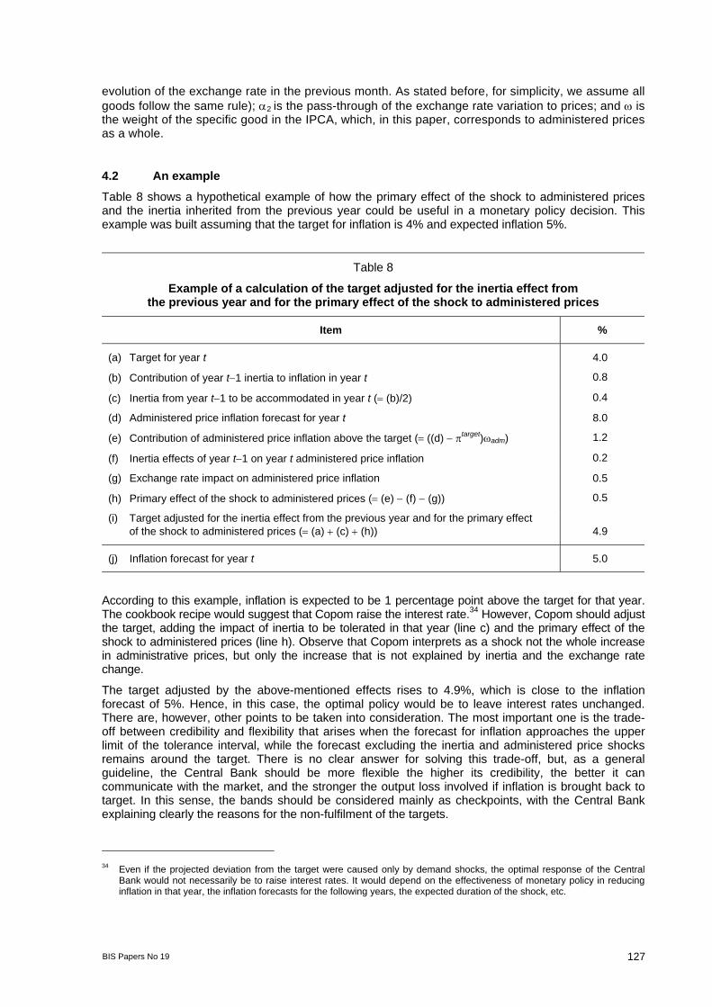
Table 8 shows a hypothetical example of how the primary effect of the shock to administered prices and the inertia inherited from the previous year could be useful in a monetary policy decision. This example was built assuming that the target for inflation is 4% and expected inflation 5%.

Table 8

Example of a calculation of the target adjusted for the inertia effect from the previous year and for the primary effect of the shock to administered prices

Item %

(a) Target for year t 4.0

(b) Contribution of year t−1 inertia to inflation in year t 0.8

(c) Inertia from year t−1 to be accommodated in year t (= (b)/2) 0.4

(d) Administered price inflation forecast for year t 8.0

(e) Contribution of administered price inflation above the target (= ((d) − πtarget)ωadm) 1.2

(f) Inertia effects of year t−1 on year t administered price inflation 0.2

(g) Exchange rate impact on administered price inflation 0.5

(h) Primary effect of the shock to administered prices (= (e) − (f) − (g)) 0.5

(i) Target adjusted for the inertia effect from the previous year and for the primary effect of the shock to administered prices (= (a) + (c) + (h)) 4.9

(j) Inflation forecast for year t 5.0

According to this example, inflation is expected to be 1 percentage point above the target for that year. The cookbook recipe would suggest that Copom raise the interest rate.34 However, Copom should adjust the target, adding the impact of inertia to be tolerated in that year (line c) and the primary effect of the shock to administered prices (line h). Observe that Copom interprets as a shock not the whole increase in administrative prices, but only the increase that is not explained by inertia and the exchange rate change.

The target adjusted by the above-mentioned effects rises to 4.9%, which is close to the inflation forecast of 5%. Hence, in this case, the optimal policy would be to leave interest rates unchanged. There are, however, other points to be taken into consideration. The most important one is the trade-off between credibility and flexibility that arises when the forecast for inflation approaches the upper limit of the tolerance interval, while the forecast excluding the inertia and administered price shocks remains around the target. There is no clear answer for solving this trade-off, but, as a general guideline, the Central Bank should be more flexible the higher its credibility, the better it can communicate with the market, and the stronger the output loss involved if inflation is brought back to target. In this sense, the bands should be considered mainly as checkpoints, with the Central Bank explaining clearly the reasons for the non-fulfilment of the targets.

34 Even if the projected deviation from the target were caused only by demand shocks, the optimal response of the Central

Bank would not necessarily be to raise interest rates. It would depend on the effectiveness of monetary policy in reducing inflation in that year, the inflation forecasts for the following years, the expected duration of the shock, etc.


5. Institutional design of inflation targeting

The inflation targeting framework has to be designed in such way that the conduct of monetary policy is oriented consistently towards the fulfilment of targets, but at the same time takes into account the limits for achieving this. Inflation is not totally under the control of the monetary authority, and output costs have to be considered. There are various reasons for the non-fulfilment of targets. The first relates to the models used by central banks: model misspecification, uncertainty concerning the estimated coefficients, possible structural breaks, existence of variables that are difficult to model, etc. The second is the presence of unexpected shocks in the economy. The third is the presence of lags in the effects of monetary policy.

We stress four issues involved in the institutional design of inflation targeting: (i) the choice of price index (core versus headline inflation); (ii) the inclusion or not of escape clauses; (iii) the size of the tolerance intervals (bands); and (iv) the horizon and criteria used for the targets.35 Besides these issues, it is important to note the current gap in the Brazilian institutional framework represented by the absence of central bank independence. Central bank independence has been implemented in several countries, and is an important element for consolidating a policy oriented towards price stability.

5.1 “To core or not to core”

The use of some measure of core inflation has been justified on the grounds that a measure of inflation that is less sensitive to temporary price movements and more reflective of the long-term trend is necessary. Monetary policy should not target a variable that is subject to temporary movements. A core inflation measure is also justified based on the argument that a measure of inflation that is less sensitive to supply shocks, such as oil prices shocks, is necessary.

There are different measures of core inflation. The most common are the exclusion method and the trimmed mean method. The first usually excludes some items such as food, oil by-product and other energy prices because these prices present high seasonality and are often subject to supply shocks. The symmetric trimmed mean core excludes the items presenting the highest and the lowest change in the period. The items are ordered according to their change. The items excluded are those whose accumulated weight from the top of the list reaches some threshold, say 20% or 30%, and those following the same criterion from the bottom of the list.36

In Brazil, the change in relative prices has motivated the discussion of the adoption of a core inflation measure, in particular a measure that would exclude administered prices. Nowadays, only a few countries target a core inflation measure, for example Canada and Thailand, which use core by exclusion. We do not include in this group countries such as the United Kingdom and South Africa, which use an inflation measure that excludes only mortgage interest rates. In this case, the motivation for the adoption of an exclusion index is different: increases in interest rates, via mortgage rates, positively affect the headline inflation rate. Actually, the international experience has pointed to the use of headline indices: Australia, New Zealand and the Czech Republic abandoned the use of core inflation measures in 1998, 1999 and 2002, respectively. Other countries, such as Colombia, Iceland, Israel, Mexico, Peru, Poland, Sweden and Switzerland also use headline inflation (Ferreira and Petrassi (2002)).

The main argument against the use of core inflation is that it is less representative of the loss of the purchasing power of money. Agents are concerned about the whole basket of consumption. In

35 For different international experiences in terms of these four items, see Ferreira and Petrassi (2002) and Mishkin and

Schmidt-Hebbel (2002). 36 The sample of the variations of the inflation rate components is ordered {x1, …, xn} with their respective weights {w1, …, wn}.

The symmetric trimmed mean is obtained from ,10021/1 ∑

α∈α

α−=

Iiii xwx where α is the threshold,

−<<=

ααα 100100

1| iWiI , Iα is the set of the components to be considered in the computation of the trimmed

mean with α%, and Wi is the accumulated weight up to ith component (Figueiredo (2001)).


the Brazilian case, exclusion of the administered items would imply leaving out more than 30% of the representative consumption basket. In this sense, private agents may question a monetary policy that is not concerned about the overall consumer price index.

Furthermore, in the Brazilian case, on some occasions during the 1970s and 1980s, the government excluded some items from the headline index on an ad hoc basis in order to reduce the official inflation rate, or even changed the official index. As a result, agents in Brazil tend to be reluctant to accept an index that excludes some items because it reminds them of these changes in the past.

The adoption of a trimmed mean core in turn would imply a great loss in terms of communicability. The basket that comprises the index is not known a priori: it depends on the evolution of prices. Furthermore, the choice of the threshold is not trivial, and is necessary to smooth some prices whose adjustments take place only from time to time.37 The Central Bank of Brazil uses a 20% symmetric trimmed mean core that includes the smoothing of eight items.38 Graph 13 presents the monthly headline (IPCA) and core inflation rates. The core measure is considerably less volatile than the headline. The standard deviation of core inflation is 0.28 and that of headline inflation 0.42 (sample: 1996:01-2002:08).

Graph 13

Headline and core inflation In percentages per month

-0.5

0

0.5

1

1.5

2

Jan

96

May

96

Sep

96

Jan

97

May

97

Sep

97

Jan

98

May

98

Sep

98

Jan

99

May

99

Sep

99

Jan

00

May

00

Sep

00

Jan

01

May

01

Sep

01

Jan

02

May

02

Headline inflation Core inflation

Nevertheless, the trimmed mean core has been shown to play an important role as predictor of inflation trend. Table 9 shows Granger causality tests between core inflation and headline inflation.39 We find that core inflation Granger causes headline inflation, that is, core inflation conveys information about future inflation (beyond that contained in past inflation), and headline inflation does not Granger cause core inflation. Therefore, core inflation can be used as a useful source of information about future inflation.

37 The discontinuous adjustments tend to be larger than the average. Therefore, in the absence of smoothing, these items

would be systematically excluded. 38 See Figueiredo (2001) for an evaluation of different core measures for Brazil. 39 See also Figueiredo and Staub (2002). Figueiredo (2001) found that the core measure has the “attractor” property as well.


Table 9

Granger causality test: core inflation and headline inflation (IPCA) Sample: 1996:01-2002:06

One lag Two lags Null hypothesis

F-statistic P-value F-statistic P-value

Core inflation does not Granger cause headline inflation 4.83 0.0311 7.14 0.0015

Headline inflation does not Granger cause core inflation 0.04 0.8479 0.98 0.3797

5.2 Escape clauses

Since the inflation rate is subject to several factors that are beyond the control of monetary policy, the success of the conduct of monetary policy should not be judged exclusively in terms of the fulfilment or not of the inflation targets. Under some circumstances, such as significant supply shocks, the Central Bank cannot avoid the inflationary impact of the shock because of the presence of lags in the effects of monetary policy or should not avoid it because of the associated output costs.

In the case of escape clauses included in the inflation targeting framework, it is set in advance of the circumstances under which the central bank can justify the non-fulfilment of targets. The inflation target design in New Zealand, South Africa, the Czech Republic and Switzerland includes escape clauses (Ferreira and Petrassi (2002)). In New Zealand, they can be invoked in the case of unpredictable events that can affect the inflation rate, such as natural disasters, and change in commodity prices and indirect tax rates. In South Africa, escape clauses include significant change in terms of trade, natural disasters, and interruption of external capital flows. Besides significant changes in international prices and agricultural production, natural disasters, and change in indirect tax rates, escape clauses in the Czech Republic comprise changes in regulated prices that affect headline inflation by more than 1-1.5 percentage points, and large changes in the exchange rate not related to domestic monetary policy. In Switzerland, escape clauses refer to change in the exchange rate and the prices of some items such as oil and imported goods.

There is clearly a trade-off in the adoption of escape clauses in the framework. Their inclusion allows a better assessment of the conduct of the Central Bank, and may avoid excessive responses from monetary policy that could otherwise occur. However, their adoption may signal that the monetary authority will be lenient towards some inflationary pressures, and their excessive use can affect the credibility of the regime.

In the Brazilian case, since the regime is still relatively new, and its credibility is still under construction, the adoption of escape clauses could negatively affect its credibility. Furthermore, the tolerance intervals should be enough to accommodate most of the shocks that the economy is subject to.

5.3 Tolerance intervals (bands)

The limits of the forecasting models, the possibility of unexpected shocks hitting the economy, and the presence of lags in the effects of monetary policy justify either the use of tolerance intervals for the point targets or the use of range targets in the absence of point targets in most of the inflation targeting countries. The size of the bands varies across countries, going from 1 percentage point in Australia and Israel to 3 percentage points in South Africa, 3.5 in Iceland, and 4 in Brazil for 2002 and 5 for 2003 and 2004.

The size of the bands should be large enough to allow the inflation rate to be within them in most circumstances, but at the same time they are not supposed to be too large to avoid a lenient conduct of monetary policy. The size of the bands has to be established according to the importance of the three factors mentioned above: it depends on the limits of the forecasting models, the frequency and


magnitude of the shocks that the economy is subject to, and the lag length of the effects of monetary policy. In the Brazilian economy, it is clear that the first two factors lead to a larger band size. First, other economies can use models estimated using a large sample because they have a much longer history of stability, and in many cases the inflation targeting regime has been adopted over a longer period.40 As a result, the forecast model can be estimated more precisely. In Brazil, the dynamics of inflation in the high-inflation period are markedly different from those in the low-inflation period. As a consequence, most of the estimations that model inflation have to start after June 1994. Moreover, with just three years of inflation targeting, possible structural breaks in the relationships are not easily found. Second, the Brazilian economy has been hit by frequent and large shocks. Most of them are related to its position as an emerging market economy - high volatility of country risk premium and of the exchange rate - and to some structural transformations that led to a change in relative prices. The volatility of the inflation rate and exchange rate in Brazil is still one of the highest in inflation targeting economies.

As we saw in previous sections, the exchange rate depreciation accounted for 38% and 48% of the inflation rate in 2001 and January-August 2002, respectively. Furthermore, exchange rate shocks explain 24.9% and 32.8% of the 12-month ahead forecast error variance of the inflation rate considering samples for the whole Real Plan period and for the inflation targeting period, respectively. The upper limit of the tolerance interval in 2001 was not enough to accommodate the shocks. Taking into account these factors affecting the band size, the National Monetary Council (CMN) has enlarged the tolerance intervals from 2 to 2.5 percentage points above and below the central targets for 2003 and 2004.

5.4 Establishment of targets and target horizon

The inflation targets have to be set taking into account both the long-term goal of price stability and the conditions for their achievement. If the actual or expected inflation rate is above the long-term goal, the targets have to be set in such a way that the inflation rate converges to it. However, it is necessary to take into consideration the associated output costs, and some country specificities that may lead to a medium-term inflation rate goal above a long-term one.

The length of the target horizon also has implications for the magnitude of the response of monetary policy to shocks. The longer the target horizon, the smaller the effects of current shocks in expected inflation for the target horizon. As a consequence, monetary policy tends to respond less to shocks.

The targets in Brazil are set in June by the CMN for the end of the calendar year two years ahead. The initial targets were established taking into account the domestic currency depreciation of the beginning of 1999, and aiming at reducing the inflation rate to low levels. In June 1999, the targets were established at 8%, 6% and 4% for 1999, 2000 and 2001, respectively, and, in June 2000, at 3.5% for 2002. In principle, inflation targets should not be changed to avoid loss of credibility. Nevertheless, the continuous pursuit of targets that are perceived in advance as having low achievability reduces the credibility of the Central Bank. Taking into account this balance of risks, the CMN decided in June 2002 to revise upwards the target for 2003 from 3.25% to 4%, and set the target at 3.75% for 2004. We consider that private agents in general have positively appraised the revision. Insisting on an unrealistic target would have negatively affected the credibility of monetary policy.

6. Conclusions

The inflation targeting regime in Brazil is relatively new, but has proved to be important in achieving low inflation rate levels even in a context of large shocks. The presence of a central bank committed to achieving preannounced inflation targets has worked as an important coordinator of expectations and generated a more stable inflation scenario. The pursuit of the goal, and the significant increase in the transparency that has marked the conduct of monetary policy - including the release of the minutes of

40 Since there is a transition period of learning, possible structural changes with the new regime can be found more easily with

a larger sample.


Copom meetings seven days after the event and of the quarterly Inflation Report - have helped develop awareness of the importance of the price stability commitment.

In this period, the regime has faced many challenges, including the construction of credibility - still under way - a change in relative prices, and exchange rate volatility. Dealing with them has required a large effort on the part of the Central Bank, which itself has also learned substantially and improved the system. The Central Bank has reacted strongly to inflation expectations, consistent with the inflation targeting framework. Market expectations have behaved in a controlled way, even in the presence of inflationary shocks. The estimations also indicate a reduction in the degree of inflation persistence and in the volatility of output and inflation.

The increase in administered prices and the exchange rate depreciation have exerted significant inflationary pressures. The Central Bank has developed a methodology to estimate the different sources of inflation, which has been used in the conduct of monetary policy.

Several issues comprise the institutional design of the inflation targeting framework. The conclusions pointed to the maintenance of headline inflation as the target and to the enlargement of the tolerance intervals (adopted for 2003 and 2004).

References

Bogdanski, J, A A Tombini and R C Werlang (2000): “Implementing inflation targeting in Brazil”, Working Paper Series, no 1, Central Bank of Brazil, July.

Bogdanski, J, P S de Freitas, I Goldfajn and A A Tombini (2001): “Inflation targeting in Brazil: shocks, backward-looking prices, and IMF conditionality”, Working Paper Series, no 24, Central Bank of Brazil, August.

Calvo, G and C Reinhart (2002): “Fear of floating”, Quarterly Journal of Economics, vol 117, no 2, May, pp 379-408.

Clarida, R, J Galí and M Gertler (1998): “Monetary policy rules in practice: some international evidence”, European Economic Review, vol 42, pp 1033-67.

——— (1999): “The science of monetary policy: a new Keynesian perspective”, Journal of Economic Literature, vol XXXVII, no 4, pp 1661-707.

——— (2000): “Monetary policy rules and macroeconomic stability: evidence and some theory”, Quarterly Journal of Economics, February.

Silva, M E A da and M S Portugal (2002): Inflation targeting in Brazil: an empirical evaluation, mimeo.

Freitas, P S de, A Minella and G Riella (2002): “Metodologia de cálculo da inércia inflacionária e dos efeitos dos choques dos preços administrados”, Notas Técnicas do Banco Central do Brasil, no 22, July (English translation in Banco Central do Brasil (2002), Inflation Report, vol 4, no 2, pp 123-8, June).

Favero, C A and F Giavazzi (2002): Why are Brazil’s interest rates so high, mimeo.

Ferreira, T P and M B S Petrassi (2002): Regime de metas para a inflação: resenha sobre a experiência internacional, Central Bank of Brazil, mimeo.

Figueiredo, F M R (2001): “Evaluating core inflation measures for Brazil”, Working Paper Series, no 14, Central Bank of Brazil, March.

——— (2002): Os preços administrados e a inflação medida pelo IPCA, Central Bank of Brazil, mimeo.

Figueiredo, F M R and R B Staub (2002): “Evaluación y combinación de mediciones de inflación de base para Brasil”, Monetaria, Cemla, pp 29-50, January-March.


Goldfajn, I and S R C Werlang (2000): “The pass-through from depreciation to inflation: a panel study”, Working Paper Series, no 5, Central Bank of Brazil, Brasilia.

Hausmann, R, U Panizza and E Stein (2001): “Why do countries float the way they float”, Journal of Development Economics, vol 66, no 2, pp 387-414.

Kuttner, K N and A S Posen (1999), Does talk matter after all? Inflation targeting and central bank behavior, mimeo.

Mishkin, F (2000): “Inflation targeting in emerging market countries”, NBER Working Paper Series, no 7618, Cambridge MA.

Mishkin, F and K Schmidt-Hebbel (2002): “A decade of inflation targeting in the world: what do we know and what do we need to know?”, in N Loayza and R Soto (eds), Inflation targeting: design, performance, challenges, Central Bank of Chile, pp 171-219.

Muinhos, M K (2001): “Inflation targeting in an open financially integrated emerging economy: the case of Brazil”, Working Paper Series, no 26, Central Bank of Brazil, August.

Schmidt-Hebbel, K and A Werner (2002): “Inflation targeting in Brazil, Chile, and Mexico: performance, credibility and the exchange rate”, Working Paper, no 171, Central Bank of Chile, July.

Sims, C A, J H Stock and M W Watson (1990): “Inference in linear time series models with some unit roots”, Econometrica, vol 58, no 1, 113-44, January.

Taylor, J B (1993), “Discretion versus policy rules in practice”, Carnegie-Rochester Conference Series on Public Policy, vol 39, 195-214.

Watson, M W (1994): “Vector autoregression and cointegration”, in R F Engle and D L McFadden (eds), Handbook of econometrics, vol IV, Elsevier, Amsterdam, pp 2844-915.

inflation targeting in brazil: lessons and challenges · inflation targeting in brazil: lessons and...

Documents