inflation and long run growth
TRANSCRIPT

8/10/2019 Inflation and Long Run Growth
http://slidepdf.com/reader/full/inflation-and-long-run-growth 1/39
Macroeconomic Dynamics, 16, 2012, 94–132. Printed in the United States of America.doi:10.1017/S1365100510000453
INFLATION AND GROWTH IN THELONG RUN: A NEW KEYNESIANTHEORY AND FURTHERSEMIPARAMETRIC EVIDENCE
ANDREA VAONA
University of Veronaand Kiel Institute for the World Economy
This paper explores the influence of inflation on economic growth both theoretically and
empirically. We propose to merge an endogenous growth model of learning by doing with
a New Keynesian one with sticky wages. We show that the intertemporal elasticity of
substitution of working time is a key parameter for the shape of the inflation–growth
nexus. When it is set equal to zero, the inflation–growth nexus is weak and hump-shaped.
When it is greater than zero, inflation has a sizable and negative effect on growth.
Endogenizing the length of wage contracts does not lead to inflation superneutrality in the
presence of a fixed cost of wage resetting. Adopting various semiparametric andinstrumental-variable estimation approaches on a cross-country/time-series data set, we
show that increasing inflation reduces real economic growth, consistent with our
theoretical model with a positive intertemporal elasticity of substitution of working time.
Keywords: Inflation, Growth, Wage Staggering, Learning by Doing, Semiparametric
Estimator
1. INTRODUCTION
This paper offers a new theoretical model and new empirical evidence on the
connection between inflation and growth.
In the theoretical part, we show that changes in the inflation rate can produce
permanent changes in the growth rate of output—even though the model here
proposed contains no money illusion, no permanent nominal rigidities, and no
departure from rational expectations. We do so by extending the model by Graham
and Snower (2004) from the inflation–output level domain to the inflation–output
growth one. As a consequence, we merge an endogenous growth model of learning
I would like to thank Guido Ascari, Luigi Bonatti, and two anonymous referees for insightful comments. Dennis
Snower was extremely supportive and helpful with a previous version of this paper. The usual disclaimer
applies. Address correspondence to: Andrea Vaona, Department of Economic Sciences, University of Verona,
Palazzina 32 Scienze Economiche—ex Caserma Passalacqua, Viale dell’Universita 4, 37129 Verona, Italy; e-mail:
c 2011 Cambridge University Press 1365-1005/11 94

8/10/2019 Inflation and Long Run Growth
http://slidepdf.com/reader/full/inflation-and-long-run-growth 2/39
INFLATION AND GROWTH IN THE LONG RUN 95
by doing with a New Keynesian one with sticky wages, making it possible to
explore how the effect of inflation on output growth is connected not only to the
direct effects of inflation on capital accumulation, but also to indirect ones passing
through the labor market.In this context, when money supply grows in the presence of temporary nominal
frictions (in the form of staggered nominal contracts), nominal adjustments never
have a chance to work themselves out fully. Thus, in an endogenous-growth
context, changes in money growth affect the marginal product of capital and
thereby the rate of economic growth.
The basic intuition for the model here proposed can be described as follows:
• When nominal wage contracts are staggered, current contract wages depend
on the current and future prices that prevail over the contract period. The
current contract wage is affected more by current prices than by expected
future prices, due to time discounting.
• The higher is the rate of money growth, the faster prices rise, and the more
the contract wage lags behind the current price level. Thus the lower is the
average real wage over the contract period. Consequently, the more labor is
demanded by firms.
In our endogenous growth model, an increase in the labor input raises the
marginal product of capital, leading to faster economic growth. There is, however,
an important countervailing effect:
• As money growth—and consequently inflation—increases, relative prices
become more volatile; i.e., the real wage varies more over the contract period,
because the nominal wage of each cohort is constant over the contract period,
whereas the aggregate price level rises gradually through time.
• This real wage volatility induces employment fluctuations, i.e., “employment
cycling.” Because there are diminishing returns to labor, this is inefficient,
leading to a reduction in the marginal product of capital and therefore in
output growth.1
These influences imply a negative long-run relation between inflation and output
growth.
We show, in a numerical example, that, when the intertemporal elasticity of
substitution of working time is set to zero, the discounting effect is dominant at
low money growth rates, whereas the employment cycling effect is dominant at
high money growth rates. By implication, the long-run relation between inflation
and output growth is backward-bending: growth rises with inflation at low inflation
rates, but falls with inflation at high inflation rates.
However, allowing for a positive intertemporal elasticity of substitution of working time, inflation has a negative impact on growth, because households,
having a greater preference for labor supply smoothing, respond to increases in
money growth—which entail more employment cycling—by raising their wage,
reducing employment and output growth.

8/10/2019 Inflation and Long Run Growth
http://slidepdf.com/reader/full/inflation-and-long-run-growth 3/39
96 ANDREA VAONA
Finally, endogenizing the length of the labor contract reduces the strength of
the effect of inflation on growth, but, in the presence of a fixed cost to wage
resetting, the negative effect of inflation on growth does not disappear. This is
because households can reduce labor cycling by paying the wage-resetting costmore often. So they choose wage flexibility only for a low level of this cost. The
welfare implications of these different model parameterizations are also discussed
in the paper.
The empirical part of the paper is mainly based on semiparametric estimation
methods applied to a cross-country/time-series data set, similarly to Vaona and
Schiavo (2007). However, we follow a different research strategy. We first use
various model selection criteria for semiparametric power series estimation ap-
proaches. Then we check whether our results have an endogeneneity bias and we
conduct various subsample stability tests. Finally, instead of adopting a Nadaraya–Watson kernel estimator, we use a local linear one with a variable window width.
Fan and Gijbels (1992) list a number of advantages of the latter estimator over
the former one. In particular, it does not lose precision near the boundary of the
observation interval (boundary effects). We find that higher inflation just harms
real economic growth. The empirical results we obtain help us to choose our
preferred calibration for the theoretical model here proposed.
The paper is organized as follows. Section 2 relates our contribution to the
existing literature. Section 3 presents the underlying model. Section 4 sketches
the model solution, which is illustrated in detail in Appendices A and B. Section5 contains our results regarding the relations between inflation and growth and
between inflation and welfare. Section 6 generalizes households’ preferences and
endogenizes the frequency of nominal adjustments. Section 7 shows our empirical
results and Section 8 concludes.
2. RELATION TO THE LITERATURE
2.1. Theoretical Literature
With the exception of a few recent studies, the theoretical literature has mainly
produced models where inflation has a negative impact on growth.
One of the first theoretical studies concerning inflation and output is Tobin
(1965), according to which inflation is beneficial to the output level because it
lowers the interest rate and therefore the opportunity cost to invest. This increases
the capital–labor ratio and therefore output.2 Stockman (1981) pointed to the
possible existence of an inverse Tobin effect, whereby an increase in the inflation
rate causes the capital stock to decrease, supposing a cash in advance constraint
for capital accumulation and given that inflation raises the cost of money holding.More recently, the literature has shifted from the level of output to the output
growth rate and from Solow models to endogenous growth ones. Gillman and
Kejak (2005a) proposed to distinguish between physical capital models, labeled as
Ak , human capital ones, labeled as Ah, and combined models, with both human and

8/10/2019 Inflation and Long Run Growth
http://slidepdf.com/reader/full/inflation-and-long-run-growth 4/39
INFLATION AND GROWTH IN THE LONG RUN 97
physical capital. The results have been mixed. Some contributions have produced
insignificant long-run inflation–growth effects, such as the Ak models of Ireland
(1994) and Dotsey and Sarte (2000) and the combined model of Chari et al.
(1996). Other contributions have produced a negative and significant inflation–growth effect, such as the Ak models of Haslag (1998) and Gillman and Kejak
(2004), the Ah model of Gillman et al. (1999), and the combined model of Gomme
(1993) and that of Gillman and Kejak (2002, 2005b). Gillman and Kejak (2005a)
propose a model that nests most of the models advanced before. Their result is that
in the Ak model inflation works as a tax on physical capital, implying a negative
Tobin (1965) effect, whereas in the Ah model inflation works as a tax on human
capital, implying a positive Tobin (1965) effect. Finally, in the combined model,
inflation works more like a tax on human capital than on physical capital, implying
a positive Tobin (1965) effect.Within a pecuniary–transaction costs model, Zhang (2000) showed that an
increase in money growth leads to lower steady-state production inputs, consump-
tion, and real money balances.
Finally, Gylfason and Herbertsson (2001) proposed to insert real money bal-
ances into the production function, as a proxy of the effect of financial depth on
production [about which see King and Levine (1993); Levine (1997); Gylfason
and Zoega (2006)], and they found a negative effect of inflation on growth through
three channels: it lowers the real interest rate and therefore savings, it reduces
efficiency by driving a wedge between the returns to real and financial capitals,and, finally, it reduces financial depth, harming output.
In Wang and Yip (1992), inflation is negatively related to growth, because
a reduction in real balances arising from an increase in the rate of monetary
growth raises transaction time and therefore transaction costs. In contrasts Mino
and Shibata (1995), in an overlapping-generations framework, show that inflation
may have a redistributive impact from one generation to the other and foster
capital accumulation. Bonatti (2002a, 2002b) argues that, when multiple balanced-
growth paths exist in a nonmonetary economy, inflation targeting cannot resolve
the resulting indeterminacy, whereas a fixed–monetary growth rule can do it, andit also determines the growth path of the economy. Furthermore, a restrictive
monetary policy may select a lower growth path rather than a more expansive one.
In Paal and Smith (2001), the relationship between money growth and real
growth is shown to be characterized by a threshold. At low money-growth rates,
banks perceive a small opportunity cost in detaining reserves instead of lending
funds for investments. As money growth rises, the nominal interest rate rises
too, increasing the opportunity cost of holding reserves and spurring lending and
therefore investment and growth. When the nominal interest rate grows beyond
a certain threshold level, credit rationing badly affects lending, reducing capitalaccumulation and growth. Also, Bose (2002) is concerned with the impact of
inflation on growth passing through the credit market. This paper argues that,
under asymmetric information between lenders and borrowers, there might be
two lending regimes. In the former, high- and low-risk borrowers are separated by

8/10/2019 Inflation and Long Run Growth
http://slidepdf.com/reader/full/inflation-and-long-run-growth 5/39
98 ANDREA VAONA
credit rationing (rationing regime). In the latter one, separation takes place through
costly screening (screening regime). A rise in the inflation rate increases the cost of
screening or the incidence of credit rationing, or it may even produce a change from
the screening to the rationing regime. All these three effects are harmful to growth.On the other hand, Funk and Kromen (2005, 2006) investigated the connec-
tion between inflation and growth in a Schumpeterian framework with short-run
price rigidity. They also found a hump-shaped inflation–growth locus due to the
distortionary effects produced by inflation on the incentive to innovate.
It is possible to conclude that the theoretical literature has focused on the effect of
inflation on growth passing through the accumulation of either human or physical
capital, through the credit market or through the product market. This study,
instead, deals with the effect of inflation on real growth passing through the labor
market in the presence of wage staggering. Furthermore, this study gives differentinsights into the inflation–growth nexus than Funk and Kromen (2005, 2006) as
we use a learning-by-doing model and not a Schumpeterian framework, wage-
staggering and not price-staggering, and, more importantly, labor supply is not
exogenously given, but determined by the optimizing behavior of economic agents.
Temple (2000) offers a broader review of the theoretical literature.
2.2. Empirical Literature
The literature review that follows gives special weight to studies on the inflation–growth nexus after 2000, as Bullard (1999) and Temple (2000) offered two surveys
of previous work. For studies before 2000, only the key ones are mentioned
hereafter.
Regarding the time-series literature, Bullard (1999) and Temple (2000) agree
that, being mainly based on unit root testing, its results might be questionable due
to the low power of these tests in finite samples. One of its main results is that
inflation and growth are not connected in the long run, given that the former would
be nonstationary and the latter stationary.3 The presence of a unit root in inflation
might be reassessed considering that many studies of the inflation-persistencenetwork of the ECB found that, allowing for structural breaks in the mean of the
inflation process, inflation appears to be stationary as well [Altissimo et al. (2006)].
Many cross-sectional and panel-data studies found a nonlinear relationship
between inflation and real growth. Gylfason and Herbertsson (2001) refer to
various studies pointing out that an increase in inflation from 5% to 50% decreases
the real growth rate. However, they found that this effect is nonlinear and that
inflation rates below 10% are positively correlated with growth, but the opposite
holds for inflation rates above 10%.
Similar results were found by Chari et al. (1996) and Barro (2001). From theformer study it would result that an increase in inflation from 10% to 20% would
decrease growth by an amount ranging from 0.2 to 0.7%. Kahn and Senhadji
(2001) found the threshold to be around 1% for industrialized countries and 11%
for developing ones. The results of Ghosh and Phillips (1998) would point it to

8/10/2019 Inflation and Long Run Growth
http://slidepdf.com/reader/full/inflation-and-long-run-growth 6/39
INFLATION AND GROWTH IN THE LONG RUN 99
be at 2.5%, Judson and Orphanides (1999) at 10%, and Pollin and Zhu (2006) at
about 13%–15%.
A threshold effect was also found by Thirlwall and Barton (1971) at an annual
inflation rate ranging from 8% to 10%. A similar value was suggested by Sarel(1996) as well. Gylfason (1991) found that economies with inflation above 20%
grew less rapidly than economies with inflation below 5% a year. Bruno and
Easterly (1998) report that inflation rates above 40% a year for at least two years
in a row are generally harmful to growth. Also, Fischer (1993) noted the existence
of a positive relationship at low inflation rates and a negative one as inflation
rises. Burdekin et al. (2004) found that, for industrialized countries, inflation rates
below 8% have an insignificant effect on growth and a negative one above that
rate. In developing countries, inflation harms growth above 3%. However, above
50%, the marginal cost of inflation decreases substantially. Finally, Vaona andSchiavo (2007) used both nonparametric and semiparametric instrumental variable
estimators, which have the advantage of letting the data speak as much as possible.
They showed that, for developed countries, low inflation rates have hardly any real
effect and high inflation rates have negative real effects. For developing countries,
they found that too high variability does not allow to reach clear-cut results.
Guerrero (2006) used previous hyperinflationary experience as instrument for
inflation, finding that inflation has a negative impact on growth. Arai et al. (2004),
using dynamic panel data methods on a data set of 115 countries over the period
1960–1995, did not find any evidence that inflation is harmful to growth. On thecontrary, the negative correlation between inflation and growth can be explained
by oil price shocks. However, Kim and Willett (2000), using cross-country/time-
series data, found that the negative effect of inflation on growth is greater in
developed countries than in developing ones and that the inclusion of oil supply
shocks in the model weakens the inflation–growth nexus, which, however, does
not disappear.
Haslag and Koo (1999), Boyd et al. (2001), and Andres et al. (2004) focused on
the interconnections between inflation, financial development, and growth. The
first two studies support the validity of the growth–financial development link butnot of the inflation–growth one. On the other hand, Andres et al. (2004) challenge
the importance of financial markets in understanding the impact of inflation on
growth.
All in all, it is possible to state that high inflation is detrimental to growth, but
there are some chances that a low inflation rate might have a positive impact on
growth, though how low is a question the literature has had many difficulties in
answering.
3. A MODEL OF NOMINAL RIGIDITIES AND ENDOGENOUS GROWTH
In our analysis, the nominal rigidity takes the form of staggered Taylor wage
contracts.4 Our model economy contains a continuum of households, supplying
differentiated labor, and a large number of identical firms, producing output by

8/10/2019 Inflation and Long Run Growth
http://slidepdf.com/reader/full/inflation-and-long-run-growth 7/39
100 ANDREA VAONA
means of all labor types and capital. The labor types are imperfect substitutes
in the production function, exhibiting diminishing returns to labor but increasing
returns to scale. Thus each household faces a downward-sloping labor demand
curve in the short run. The government prints money and it returns its seigniorageproceeds to households in the form of lump-sum tax rebates.
3.1. The Supply Side of the Economy
As far as the supply side of the economy is concerned, we assume the existence
of two good sectors. In the final good sector a set of perfectly competitive firms
transforms a continuum of horizontally differentiated inputs into a homogeneous
good. In the intermediate good sector a continuum of monopolistically competitive
firms produces different varieties of a horizontally differentiated good using both
labor and capital inputs. The continuum of monopolistically competitive firm,
indexed by f , is normalized on the [0, 1] interval.
We further suppose that there exist a capital and a labor market. Capital is
a homogeneous production factor. In the labor market, households belonging to
different cohorts set their wages in a monopolistically competitive environment
and sell their labor to the continuum of monopolistically competitive firms of
the intermediate good sector. The continuum of monopolistically competitive
households, indexed by h, is normalized on the [0, 1] interval.
The final good sector . In the final good sector, due to the existence of a set
of differentiated inputs with constant elasticity of substitution (θ p), the production
function assumes the form of a CES aggregator yt = ( 1
0 y
(θ p −1)/θ pf t df )θ p /(θ p −1);
namely, in the final good sector, firms just use intermediate inputs, yf t , to produce
their output, yt . Firms maximize profits subject to their production function,
max{yf t }
pt yt −
1 0
pf t yf t df
s.t. yt =
1
0
y
θ p −1
θ p
f t df
θ p
θ p −1
,
where pt is the aggregate price level and pf t is the price of the f th intermediate
input. By solving this maximization problem it is possible to get the demandfunction for each good variety:
yf t =
pf t
pt
−θ p
yt . (1)

8/10/2019 Inflation and Long Run Growth
http://slidepdf.com/reader/full/inflation-and-long-run-growth 8/39
INFLATION AND GROWTH IN THE LONG RUN 101
Furthermore, by imposing the zero-profit condition and substituting (1) into the
profit equation, it is possible to obtain the price index:
pt =
1 0
p1−θ pf t df
1
1−θ p
. (2)
The intermediate good sector . In the intermediate good sector each firm f
buys capital and labor to produce one variety of good. In so doing, it minimizes
costs subject to the constraint of its production function and it maximizes the
spread between the price it charges and its marginal cost.
Given that labor is horizontally differentiated, we apply a two-stage budgeting
approach after Chambers (1988, pp. 112–113) and Heijdra and Van der Ploeg(2002, pp. 360–363). First, firms choose their desired quantity of capital and of a
composite labor input, nf t , which is defined as follows:
nf t = N − 1
θ w −1
1 0
[nt (h)]θ w −1
θ w dh
θ wθ w −1
,
where h is the household index and θ w is the elasticity of substitution between
different labor kinds. We assume that households are grouped into N cohorts andthat there are 1/N households per cohort. It is plausible to assume that the presence
of a larger or a smaller number of cohorts does not have an impact on the efficiency
of the production process. Therefore, the term N −1/(θ w −1) avoids economies of
specialization in different labor kinds,5 which in the present setting coincide with
cohorts. Households within cohorts are symmetric and so the composite labor
input can be rewritten as follows:
nf t = N
− 1θ w −1 N −1
j =0
nj,t
N θ w −1
θ w θ w
θ w −1
, (3)
where j is the cohort index.
In the first stage of budgeting, firms solve the following problem:
min{nf t ,kf t }
wt
pt
nf t + rt kf t
s.t. yf t = (nf t kt )α (kf t )
1−α , (4)
where wt is the nominal aggregate wage rate, rt is the remuneration for capitalservices, kf t is the amount of capital used by firm f , kt is the aggregate capital
stock, and α is a parameter. Equation (4) is a typical production function with
knowledge externalities, whereby an increase in a firm’s capital stock leads to
an increase in its stock of knowledge. Assuming that each firm’s knowledge is a

8/10/2019 Inflation and Long Run Growth
http://slidepdf.com/reader/full/inflation-and-long-run-growth 9/39
102 ANDREA VAONA
public good, the aggregate increase in knowledge is proportional to the aggregate
capital stock [Barro and Xala-i-Martin (1995)].6
The first-order conditions for labor and capital are
wt
pt
= mct α(nf t kt )α−1(kf t )
1−α kt , (5)
rt = mct (1 − α)(nf t kt )α (kf t )
−α, (6)
where mct is the real marginal cost.
Having chosen the amounts of labor and capital that minimize costs, firms of the
intermediate-output sector maximize profits by maximizing the spread between
the price they charge and their marginal cost under the constraint of the demand
for the specific good variety they produce (1):
max{pf t }
pf t − mcnt
pt
yf t (7)
s.t. yf t =
pf t
pt
−θ p
yt , (8)
where mcnt is the nominal marginal cost.
By solving the problem (7)–(8), it is possible to show that the price charged byeach firm is just a markup over the real marginal cost:
pf t
pt
=θ p
θ p − 1mct . (9)
Recalling that firms are symmetric and their number is normalized to one, the
f index in nf t can be dropped, as
1 0
nf t df = nt .
In the second stage of budgeting, firms “construct” the composite labor input
optimally by choosing the amount of working time of cohort j , nj,t , solving the
following problem:
max{nj,t } N
− 1θ w −1 N −1
j =0
nj,t
N θ w −1
θ w θ w
θ w −1
(10)
s.t. wt nf t −
N −1j =0
wj,t
µj
nj,t
N
= 0. (11)
8/10/2019 Inflation and Long Run Growth
http://slidepdf.com/reader/full/inflation-and-long-run-growth 10/39
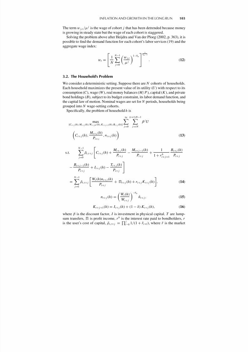
INFLATION AND GROWTH IN THE LONG RUN 103
The term wj,t /µj is the wage of cohort j that has been detrended because money
is growing in steady state but the wage of each cohort is staggered.
Solving the problem above after Heijdra and Van der Ploeg (2002, p. 363), it is
possible to find the demand function for each cohort’s labor services (19) and theaggregate wage index:
wt =
1
N
N −1j =0
wj,t
µj
1−θ w
1θ w −1
. (12)
3.2. The Household’s Problem
We consider a deterministic setting. Suppose there are N cohorts of households.
Each household maximizes the present value of its utility (U ) with respect to its
consumption (C), wage (W ), real money balances (M/P ), capital (K), and private
bond holdings (B), subject to its budget constraint, its labor demand function, and
the capital law of motion. Nominal wages are set for N periods, households being
grouped into N wage-setting cohorts.
Specifically, the problem of household h is
max{Ct +j (h),M t +j (h),W t +jN (h),Kt +j +1(h),Bt +j (h)}
∞j =0
(i+1)N −1j =iN
β
j
U Ct +j (h),
M t +j (h)
P t +j
, nt +j (h)
(13)
s.t.
N −1j =0
ρt,t +j
Ct +j (h) +
M t +j (h)
P t +j
−M t +j −1(h)
P t +j
+1
1 + r bt +j +1
Bt +j (h)
P t +j
−Bt +j −1(h)
P t +j
+ I t +j (h) −T t +j (h)
P t +j
=
N −1j =0
ρt,t +j
W t (h)nt +j (h)
P t +j
+ t +j (h) + rt +j Kt +j (h)
, (14)
nt +j (h) =
W t (h)
W t +j
−θ w
nt +j , (15)
Kt +j +1(h) = I t +j (h) + (1 − δ) Kt +j (h), (16)
where β is the discount factor, I is investment in physical capital, T are lump-
sum transfers, is profit income, r b is the interest rate paid to bondholders, r
is the user’s cost of capital, ρt,t +j =j
l=0 1/(1 + rt +l ), where r is the market
8/10/2019 Inflation and Long Run Growth
http://slidepdf.com/reader/full/inflation-and-long-run-growth 11/39
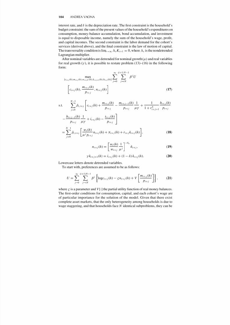
104 ANDREA VAONA
interest rate, and δ is the depreciation rate. The first constraint is the household’s
budget constraint: the sum of the present values of the household’s expenditures on
consumption, money-balance accumulation, bond accumulation, and investment
is equal to disposable income, namely the sum of the household’s wage, profit,and capital incomes. The second constraint is the labor demand for the cohort’s
services (derived above), and the final constraint is the law of motion of capital.
The transversality condition is limt →∞ t Kt +1 = 0, where t is the nondetrended
Lagrangian multiplier.
After nominal variables are detrended for nominal growth (µ) and real variables
for real growth (γ ), it is possible to restate problem (13)–(16) in the following
form:
max{ct +j (h),mt +j (h),wt +jN (h),kt +j +1(h),bt +j (h)}
∞j =0
(i+1)N −1j =iN
βj U
ct +j (h),
mt +j (h)
pt +j
, nt +j (h)
(17)
s.t.
N −1j =0
ρt,t +j
ct +j (h) +
mt +j (h)
pt +j
−mt +j −1(h)
pt +j
1
µγ +
1
1 + r bt +j +1
bt +j (h)
pt +j
−bt +j −1(h)
pt +j
1
µγ + it +j (h) −
t t +j (h)
pt +j
=
N −1j =0
ρt,t +j
wt (h)
µj pt +j
nt +j (h) + πt +j (h) + rt +j kt +j (h)
, (18)
nt +j (h) = wt (h)
wt +j
1
µj −θ w
nt +j , (19)
γ kt +j +1(h) = it +j (h) + (1 − δ) kt +j (h). (20)
Lowercase letters denote detrended variables.
To start with, preferences are assumed to be as follows:
U =
∞j =0
(i+1)N −1j =iN
βj
logct +j (h) − ς nt +j (h) + V
mt +j (h)
pt +j
, (21)
where ς is a parameter and V [·] the partial utility function of real money balances.The first-order conditions for consumption, capital, and each cohort’s wage are
of particular importance for the solution of the model. Given that there exist
complete asset markets, that the only heterogeneity among households is due to
wage staggering, and that households face N identical subproblems, they can be

8/10/2019 Inflation and Long Run Growth
http://slidepdf.com/reader/full/inflation-and-long-run-growth 12/39
INFLATION AND GROWTH IN THE LONG RUN 105
written as follows:
βj
ct +j
= λt +j ρt,t +j , (22)
γ λt +j = ρt,t +1λt +j +1(1 − δ + rt +j ), (23)
N −1j =0
nt +j βj =
θ w − 1
θ wς
N −1j =0
ρt,t +j wj,t
pt +j µj
nt +j
ct +j
, (24)
where λt +j is the detrended Lagrange multiplier.
3.3. The GovernmentFor simplicity, the government is assumed to distribute its seigniorage in the form
of lump-sum transfers to households:
mt +j − mt +j −1
1
µγ = t t +j . (25)
4. THE MODEL SOLUTION
The macroeconomic model is constituted by the equations (1), (2), (4)–(6), (9),(12), (19), and (22)–(25). The procedure for solving the model is outlined in more
detail in Appendix A.
Note that Graham and Snower (2004) showed that in steady state ρt,t +j = β j .7
Furthermore, in equilibrium there is no arbitrage between alternative assets and
so r = r b = r − δ. It is possible to obtain the solution for the steady-state growth
rate of the economy by using (4), (6), (9), (22), and (23):
γ = β 1 − δ +θ p − 1
θ p
(1 − α) (n)α. (26)
The nondetrended version of (23) implies that the law of motion of the non-
detrended Lagrangian multiplier is
t +j =
1
ρt,t +1(1 − δ + rt +j )
j
t ,
which, together with the transversality condition and the equality ρt,t +j = βj ,
imposes the restriction on the percentage growth rate of being nonnegative.
In this stage it is necessary to find the steady-state level of the composite laborinput in order to solve the model. In the Appendix we show that, assuming α = 2
3,
the composite labor input is given by the roots of the polynomial
A3n3 − 3A2Bn2 + (3AB2 − C 3)n − B 3 = 0, (27)

8/10/2019 Inflation and Long Run Growth
http://slidepdf.com/reader/full/inflation-and-long-run-growth 13/39
106 ANDREA VAONA
where A, B , and C are defined as follows:
A := 1 − βθ p − 1
θ p
(1 − α), (28)
B :=
N
1 − µ(θ w −1)
1 − µN(θ w −1)
θ p − 1
θ pα
1 − β N µN (θ w −1)
1 − βµ(θ w −1)
1 − βµθ w
1 − (βµθ w )N
θ w − 1
θ wς
×
1
N
1 − µN (θ w −1)
1 − µθ w −1
θ wθ w −1
, (29)
C := (1 − δ) (β − 1). (30)
The possibility of having multiple steady states within a learning-by-doing
model is well known in the literature [Benhabib and Farmer (1994)]. We calibratethe model using standard parameter values (β = 0.961/N , N = 52, δ = 1 −
0.921/N , θ p = 10, α = 0.67, θ w = 2) similarly to Huang and Liu (2002), Ascari
(2003), and Graham and Snower (2004). ς has been adjusted for the model to
produce realistic growth rates. Under this calibration two of the three roots of (27)
turn out to be complex numbers, which can be ruled out, being without economic
meaning. This leaves us with a unique solution for the model.
Figures 1 and 2 show how the long-run growth rate of the economy changes as
a function of θ p and θ w, setting µ = 1.02. An increase in θ p reduces monopolistic
rents in the intermediate-product market, implying a positive income effect andenhancing economic growth. This effect is captured by terms depending on θ p in
(26), (28), and (29). The same happens for θ w, even though its impact on long-run
growth is the result of a number of different mechanisms. First of all, an increase
in θ w reduces monopolistic rents on the labor market, entailing a greater labor
supply. However, due to wage staggering, this is not the complete story. Consider
the ratio between the labor demanded for cohort 0 and cohort j :
n0
nj
= µ−θ w j . (31)
An increase in θ w entails more labor cycling, which produces more inefficiencies.
This negative effect, however, does not offset the beneficial reduction of rents
leading to a net increase in the composite labor input and therefore in economic
growth.
5. THE EFFECTS OF MONETARY POLICIES
5.1. The Real Effects of Monetary Policy
Figure 3 shows that the relationship between money and real growth is clearly
nonlinear. There is a threshold: increasing the money growth rate has a tiny
positive impact on real growth up to about 2% and a negative one above this
value. As shown by Graham and Snower (2004) analyzing structural equations,

8/10/2019 Inflation and Long Run Growth
http://slidepdf.com/reader/full/inflation-and-long-run-growth 14/39
INFLATION AND GROWTH IN THE LONG RUN 107
6 7 8 9 10 11 12 13 14 15 161.5
2
2.5
3
3.5
P e r c e n t a g e r e a l g r o w t h r a t e
4
4.5
5
θ p
FIGURE 1. The effect of θ p on real growth.
2 3 4 5 6 7 8 9 10 11 125
6
7
8
9
10
11
12
θ w
P e r c e n t a g e r e a l g r o
w t h r a t e
FIGURE 2. The effect of θ w on real growth.

8/10/2019 Inflation and Long Run Growth
http://slidepdf.com/reader/full/inflation-and-long-run-growth 15/39
108 ANDREA VAONA
0 5 10 15 20 25 304.36
4.37
4.38
4.39
4.4
4.41
4.42
4.43
4.44
Percentage money growth rate
P e r c
e n t a g e r e a l g r o w t h r a t e
FIGURE 3. The effect of money growth on real growth.
the discounting and the employment-cycling effects underlie these nonlinearities.
At low inflation rates, the time-discounting effect prevails, leading to a greater
labor supply and therefore to faster capital accumulation and growth. In contrast,
at high inflation rates the employment-cycling effect is stronger, leading to less
labor demand and therefore to slower growth. The labor-cycling effect is due
to the fact that firms substitute between different kinds of labor because agentsbelonging to different cohorts have different wages, some of them being locked
into past contracts.
The analysis above, regarding how the elasticities of substitution between differ-
ent goods and different labor kinds affect the real growth rate, already gives some
insights into how they affect the long-run relationship between money growth
and real growth. Figures 4 and 5 show that the money growth–real growth locus
moves upward as either θ p or θ w increases. Under the present calibration, economic
growth appears to be much more sensitive to the structural parameters of the model
than to money growth, as the discounting and the employment-cycling effects tendto offset one another.
5.2. Optimal Monetary Policy
To individuate the optimal rate of money growth we use a specification of the
welfare function similar to Woodford (1998), Aoki (2001), and Benigno (2004),

8/10/2019 Inflation and Long Run Growth
http://slidepdf.com/reader/full/inflation-and-long-run-growth 16/39
INFLATION AND GROWTH IN THE LONG RUN 109
0 5 10 15 20 25 304.36
4.37
4.38
4.39
4.4
4.41
4.42
4.43
4.44
Percentage money growth rate
P e r c e n t a g e r e a l g r o w t h r a t e
Benchmark model
After a 0.1% increase in θ p
FIGURE 4. The effect of money growth on real growth for different values of θ p.
0 2 4 6 8 10 12
4.416
4.418
4.42
4.422
4.424
4.426
4.428
4.43
4.432
4.434
4.436
Percentage money growth rate
P e r c e n t a g e r e a l g r o w t h r a t e
Benchmark model
After a 0.1% increase in θ w
FIGURE 5. The effect of money growth on real growth for different values of θ w.

8/10/2019 Inflation and Long Run Growth
http://slidepdf.com/reader/full/inflation-and-long-run-growth 17/39
110 ANDREA VAONA
0 5 10 15 20 25 30
0.005
0
0.01
0.015
0.02
0.025
0.03
0.035
Percentage money growth rate W e l f a
r e ( %
d e v i a t i o n f r o m t h e l e v e l o f w e l f a r e w i t h f l e x i b l e p r i c e s )
FIGURE 6. The effect of money growth on welfare.
where the weight of money holdings is assumed to be so small to be negligible:
W =
∞
j =0
βj (logCt +j − ς nj t +j ).
Ct +j is growing at the rate γ ; therefore Ct +j = ct γ j .
As showed in Appendix B, maximizing W is equivalent to maximizing the
criterion
W =1
1 − β N
β
1 − β N
(1 − β)2 −
βN N
1 − β
log γ
− ς n0
1
1 − β N
1 − β N µθ w N
1 − βµθ w+
1
1 − β N log (nα − γ + 1 − δ). (32)
Figure 6 shows that money growth does not affect welfare to a great extent.
However, under the present calibration, the optimal inflation rate would be above
20%, a result that does not hold for more realistic calibrations below. This happens
because money growth affects W through four channels: the real growth rate of the

8/10/2019 Inflation and Long Run Growth
http://slidepdf.com/reader/full/inflation-and-long-run-growth 18/39
INFLATION AND GROWTH IN THE LONG RUN 111
economy, the working time of cohort zero, the term (1 − β N µθ w N )/(1 − βµθ w ),
and the initial level of consumption. The second channel can be taken to rep-
resent the labor-cycling effect,8 whereas following Graham and Snower (2004,
p. 18), the third channel can be taken to represent the time-discounting effect. Tounderstand which channel dominates, we decompose W into three terms,
W 1 =1
1 − β N
β
1 − β N
(1 − β)2 −
βN N
1 − β
log γ ,
W 2 = ς n0
1
1 − β N
1 − β N µθ w N
1 − βµθ w,
W
3 =
1
1 − β N log (nα − γ + 1 − δ),
and we compute six percentage variations:
%W 1a =W 1max − W 1ff
W ff
× 100,
%W 2a =W 2max − W 2ff
W ff
× 100,
%W 3a =W 3max − W 3ff
W ff
× 100,
%W 1b =W 1end − W 1max
W max
× 100,
%W 2b =W 2end − W 2max
W max
× 100,
%W 3b =
W 3end − W 3max
W max× 100,
where the subscript “max” indicates values taken at the maximum of W , ff the
values taken with flexible wages, and end the last computed values. After, for
instance, Wolff (2003), we further decompose %W 2a and %W 2b to isolate the
effect of n0 from that of (1 − β N µθ w N )/(1 − βµθ w ), using the fact that, for a given
variable z = b × f, one has that z2 − z1 = b∗(f 2 − f 1) + f ∗(b2 − b1), where
b∗ = (b2 + b1)/2 and f ∗ = (f 2 + f 1)/2, where 1 and 2 indicate different values
of the variables.
Under the present parameterization, %W 1a = −0.0328%, %W
2a =
−0.0715%, and %W 3a = −0.0072%, whereas %W 1b = −0.0263%,
%W 2b = −0.0292%, %W 3b = −0.0057%. So the second term in (32) ap-
pears to be the most responsive to changes in money growth. However, %W 1a
and %W 3a cannot compensate for %W 2a , though %W 1b and %W 3b can

8/10/2019 Inflation and Long Run Growth
http://slidepdf.com/reader/full/inflation-and-long-run-growth 19/39
112 ANDREA VAONA
compensate for %W 2b, eventually leading W to fall. The changes in %W 2a
and %W 2b attributable to n0 and (1 − β N µθ w N )/(1 − βµθ w ) are of about
the same magnitudes, though the latter tends to be somewhat greater. Indeed,
%W 2a = −0.0715% can be decomposed into two further percentage varia-tions: one, attributable to n0, equals −16.9854% and the other, attributable to
(1 − β N µθ w N )/(1 − βµθ w ), equals 16.9140%. For %W 2b these two changes are
equal to −5.3833% and 5.3542%, respectively.
To sum up, under the present parameterization, money growth has a tiny non-
linear effect on real growth and welfare because the time-discounting and labor-
cycling effects tend to cancel each other out. However, welfare tends to increase
up to very high inflation rates because the effects of real growth, time discounting,
and the initial level of consumption cannot completely offset the labor-cycling
effect, which leads to a welfare-enhancing deacrease in working time. We will seebelow that this result does not hold for more general preferences.
6. EXTENSIONS
6.1. Generalized Preferences
In this section we relax the hypothesis of linear preferences in labor time. And we
assume that the intertemporal elasticity of substitution of working time is equal
to φ :
U =
∞j =0
βj
log ct +j (h) − ς
n1+φ
j,t +j (h)
1 + φ+ V
mt +j (h)
pt +j
. (33)
Consequently the first-order condition of the consumer’s maximization problem
and B will respectively be as follows:
N −1
j =0
n(1+φ)j,t +j β
j =θ w − 1
θ wς
N −1
j =0
ρt,t +j wj,t
pt +j µj
nj,t +j
ct +j
, (34)
B :=
N
1 − µ(θ w −1)
1 − µN (θ w −1)
θ p − 1
θ pα
1 − β N µN (θ w −1)
1 − βµ(θ w −1)
×1 − βµ(1+φ)θ w
1 −
βµ(1+φ)θ wN
θ w − 1
θ wς
1
N
1 − µN (θ w −1)
1 − µθ w −1
θ wθ w −1
.
The welfare criterion is now
W =1
1 − β N
β
1 − β N
(1 − β)2 −
βN N
1 − β
log γ (35)
− ς n0
1
1 − β N
1 − β N µθ w (1+φ)N
1 − βµθ w (1+φ) +
1
1 − β N log (nα − γ + 1 − δ). (36)

8/10/2019 Inflation and Long Run Growth
http://slidepdf.com/reader/full/inflation-and-long-run-growth 20/39
INFLATION AND GROWTH IN THE LONG RUN 113
In our benchmark model, we set φ = 5, consistent, for instance, with Huang
and Liu (2002), but we also check the sensitivity of our results fixing φ to 2.5.
Figures 7a and 7b show the long-run relationship between inflation and growth and
the welfare level associated with different inflation rates for this new specificationof the model. Similarly to Graham and Snower (2004) for the relationship between
inflation and the level of output, this is due to the labor supply–smoothing effect.
With φ > 0, households have a greater preference for smoothing their labor
supply over the contract period. As a consequence, being adversely affected by
increases in money growth that lead to more employment cycling due to wage
staggering, they raise their wage, reducing labor demand, the aggregate quantity
of labor input, and so, output growth. The greater is φ, the steeper is the real
growth–money growth locus.
The money growth–welfare locus is now downward-sloping, as the real growth,the labor cycling and the initial consumption effects more than offset the time-
discounting effect.
6.2. Endogenizing the Length of the Labor Contract
This section is devoted to endogenizing the frequency of nominal adjustments.
As in Graham and Snower (2004), we suppose that N is set in order to maximize
households’ welfare:
maxN
∞j =0
βj
log Ct +j − ς
n1+φ
j,t +j
1 + φ− F
(37)
under (14)–(16). F is a fixed cost of changing wages.
Reasoning along the lines of Appendix B, (37) can be rewritten as
maxN
∞
j =0
N (j +1)−1
l=Nj
β l
log Ct +l − ς
n1+φ
l,t +l
1 + φ− F
. (38)
Problem (38) in the steady state is an infinite sum of N periods’ problems. There-
fore, it becomes
maxN
1
1 − β N
β
1 − β N
(1 − β)2 −
βN N
1 − β
log γ +
1
1 − β N log (nα − γ + 1 − δ)
−1
1 − β N ς n0
1
1 + φ
1 −
βµ(1+φ)θ wN
1 − βµ(1+φ)θ w−
1
1 − β N F .
The problem can be solved numerically. Again following Graham and Snower(2004), we assume that, at a 4% inflation rate, wages are set for one year. Results for
different values of F are shown in Figures 8a and 8b. First, under the assumption
F 0, endogenizing N does not lead to money superneutrality. This happens
because households have a preference against labor cycling and so for wage

8/10/2019 Inflation and Long Run Growth
http://slidepdf.com/reader/full/inflation-and-long-run-growth 21/39
0 2 4 6 8 10 12
0.5
0
1
1.5
2
2.5
3
3.5
4
4.5(a)
Percentage money growth rate
P e r c e n t a g e r e a l g r o w t h r a t e
Benchmark modelφ = 2.5
0 2 4–3
–2.5
–2
–1.5
–1
–0.5
0
Percent
W e l f a r e ( %
d e v i a t i o n f r o m t h e
l e v e l o f w e l f a r e w i t h f l e x i b l e p r i c e s )
FIGURE 7. The effect of money growth on real growth and welfare for generalized preferences. In the benc
of substitution for working time is set equal to 5.

8/10/2019 Inflation and Long Run Growth
http://slidepdf.com/reader/full/inflation-and-long-run-growth 22/39
0 1 2 3 4 5 6 7 8 9
0.5
0
1
1.5
2
2.5
3
3.5
4
4.5
(a)
Percentage money growth rate
P e r c e n t a g
e r e a l g r o w t h r a t e F = 0.1
F = 1
0 1 230
35
40
45
50
55
Perc
L e n g t h o f w a g e c o n t r a c t
FIGURE 8. The effect of money growth on real growth and on wage contract length with endogenous labelasticity of substitution for working time is set equal to 5.
8/10/2019 Inflation and Long Run Growth
http://slidepdf.com/reader/full/inflation-and-long-run-growth 23/39
116 ANDREA VAONA
flexibility, but they can achieve it only by paying more frequently F . So, in the
end, they face a trade-off and they prefer not to set N = 1. As a matter of
consequence, for F → 0, the length of the wage contract converges to 1 and
money becomes superneutral.
7. NEW SEMIPARAMETRIC EVIDENCE ON THEINFLATION–GROWTH NEXUS
The present section offers new empirical evidence on the inflation–growth nexus,
following in the footsteps of Vaona and Schiavo (2007). To obtain results compa-
rable to theirs we use the same model specifications and data set, which, on their
own, build on the work of Khan and Senhadji (2001).Our dependent variable is the growth rate of GDP in constant local currency
units. The independent variables of Specification I are the level of inflation, gross
fixed-capital formation (or gross capital formation when the former is not avail-
able) over GDP, the log of initial per capita GDP in PPP adjusted dollars, population
growth, the average schooling years in the total population aged 15 or more, and
the share of government expenditure over GDP. Specification II controls also for
the growth rate of the terms of trade and their five-year standard deviation. 9 In
both specifications we include a set of country and time dummies to control for
possible unobserved heterogeneity.We resort to different data sources. For per capita GDP and the share of gov-
ernment consumption we revert to the Penn World Tables (PWT). Our education
measure is obtained from the Barro and Lee data set on educational attainment. We
use the export and import unit value series from the IMF’s International Financial
Statistics (IFS) to build terms-of-trade data.
Our data set spans from 1960 to 1999 over 167 countries. After Temple (2000),
we experiment with different time frequencies but our baseline results are based
on five-year means.10 Missing values reduce the number of available observations
(especially for developing countries). We also drop from the sample all the observa-tions with an inflation rate above 40%, as in Kahn and Senhadji (2001).11 Our final
sample includes 85 countries and 421 observations. Of these, 119 observations
belong to 19 industrial countries. Considering the terms-of-trade variables reduces
the number of developing countries from 66 to 25, leaving developed countries
almost unaffected.
We follow a research strategy different from that of Vaona and Schiavo (2007).
First, after Li and Racine (2007, Chap. 15), we use a semiparametric power series
estimator and we look for the best-fitting model specification using several criteria.
Then we check for endogeneity bias by implementing a two-stage least-squaresestimator (2SLS) and a Hausman test. Finally, we perform various robustness
controls for our results by splitting our sample between developed and developing
countries, by using eight-year averages, and by resorting to a semiparametric local
linear estimator. This research strategy allows us to test whether an instrumental

8/10/2019 Inflation and Long Run Growth
http://slidepdf.com/reader/full/inflation-and-long-run-growth 24/39
INFLATION AND GROWTH IN THE LONG RUN 117
variable estimator is appropriate, rather than assuming it, as in Vaona and Schiavo
(2007).
Consider the following econometric model:
Y i = X 1i β + φ (X2i ) + ui ,
where Y i is the dependent variable, Xj i for j = 1, 2 are two sets of independent
variables, β is a vector of coefficients to be estimated, φ(·) is a nonlinear function of
unspecified form, i is the subscript for the ith observation, and ui is the disturbance.
We here assume that X2i is a scalar. It is possible to approximate φ(·) using a
power series function:
ps (X2i ) = Xs
2iK
s=1.
However, it is necessary to choose K . The literature has proposed severalcriteria to help this choice. Two prominent examples are the Akaike and Schwarz
parametric criteria. We also consider three nonparametric procedures: Mallows’s
CL, generalized cross validation, and leave-one-out cross validation.
Mallows’s CL consists in selecting K to minimize
N −1
N i
[Y i − X1i β − φ (X2i )]2 + 2σ 2
K
N
,
where N is the number of observations, β and φ are the estimated counterparts of β and φ, σ 2 =
N i u2
i /N , and ui = Y i − X1i β − φ(X2i ).
According to generalized cross validation, one selects K to minimizeN i [Y i − X
1i β − φ (X2i )]21 −
Kn
2 .
Finally, the leave-one-out cross validation consists of selecting K to minimize
CV K =
N i
[Y i − X1i β−i − φ−i (X2i )]2,
where β−i and φ−i are estimated after removing (Y i , X1i , X2i ).
We apply the procedures above to our data sample for both Specifications I and
II, fixing the maximum of K to 4. As shown in Table 1, the majority of the criteria
points to a first-order polynomial as the best fitting option, so we stick to it.
Next we compare our OLS estimates to the 2SLS ones by means of a Hausman
test. As in Barro (1995), we instrument inflation by its first lag. Using this instru-
ment entails assuming that it should not enter the econometric model for growth.This is consistent with our theoretical model, where there is not any delay in the
impact of money growth on real growth.12 Table 2 shows our results. Regressing
present inflation on its first lag (and on all the controls of our model) returns a
p-value of 0.00 with a t -statistic of 4.91 and an F -statistic 24.06 for Specification

8/10/2019 Inflation and Long Run Growth
http://slidepdf.com/reader/full/inflation-and-long-run-growth 25/39
TABLE 1. Model selection criteria
Whole sample: specification I Whole
Polynomial order P
Criteria 1 2 3 4 1
Mallows’s C L 4.0004 3.9954 3.9902 3.9936 2.7151 2
Generalized 4.5821 4.5882 4.5942 4.6103 3.2551 3cross validation
Leave-one-out 1.2893 1.2911 1.2889 1.2901 428.8411 429
cross validation
Akaike information 1,987.257 1,987.294 1,987.308 1,988.337 929.1067 928
criterion
Schwartz information 2,413.22 2,417.393 2,421.543 2,426.707 1,140.4 1,14
criterion

8/10/2019 Inflation and Long Run Growth
http://slidepdf.com/reader/full/inflation-and-long-run-growth 26/39
INFLATION AND GROWTH IN THE LONG RUN 119
TABLE 2. Coefficient estimates and t -statistics of the control variables
Specification I Specification II
OLS 2SLS OLS 2SLS
Inflation −0.09∗ −0.09 −0.16∗ −0.23∗
t -statistics −4.76 −1.23 −4.51 −2.15
GDP per capita −4.74∗ −4.76∗ −6.46∗ −6.57∗
t -statistics −8.25 −6.50 −7.01 −6.95
Population growth 1.50∗ 1.50∗ 0.64 0.70∗
t -statistics 9.12 8.93 1.92 2.02
Investment/GDP 0.20∗ 0.20∗ 0.30∗ 0.31∗
t -statistics 7.73 7.17 8.15 8.06
Government consumption/GDP −0.03 −0.03 −0.02 0.01t -statistics −1.30 −1.00 −0.70 0.02
Education 0.19 0.19 0.11 0.08
t -statistics 0.96 0.85 0.46 0.33
Terms of trade growth — — 0.11∗ 0.11∗
t -statistics — — 3.07 3.11
Terms of trade standard deviation — — 0.89∗ 0.86∗
t -statistics — — 2.22 2.14
First-stage F -statistic (p-value) — 0.00 — 0.00
Hausman test (p-value) — 1.00 — 1.00
Adjusted R2 0.56 0.56 0.60 0.60Observations 462 462 236 236
∗Significant at the 5% level. The models also include a set of country and time-period dummies.
I and a t -statistic of 4.65 and an F -statistic of 21.61 for Specification II. So the
instrumented variable is highly significantly correlated with its instrument and our
results should not be biased by a weak instrument problem. The Hausman test
would not reject the null that the OLS and 2SLS estimators are equal and, indeed,
for both the specifications the inflation coefficients are very close. Inflation istherefore confirmed to have a negative linear impact on growth.
To check the robustness of our results, we first split our sample between de-
veloped and developing countries (Table 3). For the latter, all the criteria point to
a linear model as the best-fitting one. For the former, instead, there is a discrep-
ancy between Specifications I and II. In the first case a fourth-order polynomial
would be selected by all the criteria but the Schwarz one, which would select a
second-order polynomial. Once the growth rate of the terms of trade and their
five-year standard deviation are added to the model, the majority of the criteria
would select a linear model. Such a discrepancy could be caused by the omissionof a relevant variable, given that the growth rate of the terms of trade is highly
significantly correlated with economic growth13 and that nonlinear terms can be
used to detect the omission of a relevant variable [see, for instance, Ramsey
(1969)].

8/10/2019 Inflation and Long Run Growth
http://slidepdf.com/reader/full/inflation-and-long-run-growth 27/39
TABLE 3. Robustness checks for model selection criteria
Developed countries: Specification I Dev
Polynomial order
Criteria 1 2 3 4 1
Mallows’s C L 1.4604 1.4246 1.3982 1.3856 1.3996
Generalized cross validation 1.7016 1.6739 1.6571 1.6568 1.7071
Leave-one-out cross validation 156.7271 153.7707 150.4885 149.8273 124.3379
Akaike information criterion 501.9681 498.8436 496.6573 495.9556 436.5977
Schwartz information criterion 610.8278 610.7271 611.5647 613.8869 540.6503
Developing countries: Specification I Deve
Polynomial order
Criteria 1 2 3 4 1
Mallows’s C L 5.1022 5.1224 5.1116 5.1242 4.2152
Generalized cross validation 6.0865 6.1377 6.1522 6.1953 6.0263
Leave-one-out cross validation 1,060.6 1,067.3 1,063.4 1,067.0 277.4053
Akaike information criterion 1,415.244 1,417.148 1,417.180 1,418.631 490.3006Schwartz information criterion 1,710.434 1,716.074 1,719.842 1,725.030 598.3198

8/10/2019 Inflation and Long Run Growth
http://slidepdf.com/reader/full/inflation-and-long-run-growth 28/39
INFLATION AND GROWTH IN THE LONG RUN 121
TABLE 4. Model selection criteria using eight-year averages
Developed countries: specification I
Polynomial order
Criteria 1 2 3 4
Mallows’s C L 0.6674 0.6745 0.6748 0.6813
Generalized cross validation 0.9851 1.0202 1.0466 1.0849
Leave-one-out cross validation 34.6133 35.7789 36.2510 37.1464
Akaike information criterion 228.6061 230.3979 231.3121 1,418.631
Schwartz information criterion 309.9811 314.2387 317.6189 321.827
Finally, Vaona and Schiavo (2007) found that a mild positive effect of inflation
on growth appears at low inflation rates in developed countries for Specification I
when eight-year means are considered instead of five-year ones. We run our model
selection criteria again for this case, but we do not find any nonlinearity in the
data, as shown in Table 4. A linear model appears to be the best-fitting one.
Our final robustness check is to compute a semiparametric local linear kernel
estimator, whose main advantage, compared to the Nadaraya–Watson one, is not
being so sensitive to boundary observations. In our context, this advantage is very
important, given that the threshold level of inflation has often been found to berather low. Using a semiparametric kernel estimator, one can obtain an estimate
of β as follows:
β =
N i=1
(X1i − m12i ) (X1i − m12i )
−1 N i=1
(X1i − m12i ) (Y i − m2i )
,
where m12i and m2i are the nonparametric estimators of m12i = E (X1i |X2i )
and m2i = E (Y i |X2i ), where E is the expectation operator. Using a local linear
estimator, one has
m2i = e 1
n−2 +
ni=1
ai K
X2i − X2
h (X2i )
a
i
−1
ai K
X2i − X2
h (X2i )
Y i ,
where ai = [1, (X2i − X2)], e1 is a column vector of the same dimension as ai,
with unity as first element and zero elsewhere, and K(·) is the kernel function
[Pagan and Ullah (1999)]. Here we use a Gaussian kernel. After Fan and Gijbels
(1992), we work with a variable bandwidth h(X2i ) = hf −1/5(X2i ), where h was
chosen to be equal to Silverman’s optimal smoothing bandwidth and f (X2i ) is akernel estimate of the density of X2i .
m12i assumes a form similar to m2i . Recall that
φ (X2i ) = E [
Y i − X1i β
|X2i ].

8/10/2019 Inflation and Long Run Growth
http://slidepdf.com/reader/full/inflation-and-long-run-growth 29/39
122 ANDREA VAONA
TABLE 5. Coefficient estimates and t -statistics of the control variables of thesemiparametric estimate of the inflation–growth nexus
Specification II Specification I:Developed eight-yearAll Developed Developing averages
GDP per cap −6.44∗ −5.54∗ −6.02∗ −4.96∗
t -statistics −7.07 −4.27 −4.34 −3.92
Population growth 0.65 1.09∗ 0.71 0.94
t -statistics 1.97 2.44 1.30 1.93
Investment/GDP 0.31∗ 0.19∗ 0.34∗ 0.17∗
t -statistics 8.33 2.90 5.20 2.58
Government −0.01 −0.10∗ 0.05 −0.08∗
consumption/GDPt -statistics −0.35 −2.61 0.69 −2.54
Education 0.10 0.45∗ −0.32 0.36
t -statistics 0.45 2.07 −0.64 1.85
Terms of trade growth 0.10∗ 0.12∗ 0.10 —
t -statistics 3.04 2.81 1.73 —
Terms of trade 0.86∗ −5.22 0.83 —
standard deviation
t -statistics 2.15 −1.41 1.37 —
∗ Significant at the 5% level. The models also include a set of country and time-period dummies.
Given our results above, we mainly focus on Specification II, as Specification I
omits a relevant variable, the growth rate of terms of trade. Parameter estimates for
the control variables are set out in Table 5. Figure 9 shows estimates of the partial
effect of inflation on growth for the whole sample, for developed countries, and
for developing ones. Once again, no threshold level of inflation can be detected,
the effect of inflation on growth appears to be just negative, and linearity is a
good approximation. Shifting to eight-year averages for developed countries andto Specification I would not change our results.
Our empirical results can shed light on the theoretical results above. Though
we cannot prove that the labor market channel highlighted by our theory is the
dominant one compared to other channels already illustrated by the literature, we
show that, assuming a non-null intertemporal elasticity of substitution of working
time, our model does not produce unrealistic results. So our empirical results help
us to select the most suitable parameterization for our model.
8. CONCLUSIONS
This paper extends the results of the New Keynesian literature with wage stag-
gering from the relation between inflation and the level of output to the inflation–
growth nexus. In this way, it is possible to explore how inflation affects growth

8/10/2019 Inflation and Long Run Growth
http://slidepdf.com/reader/full/inflation-and-long-run-growth 30/39
0 5 10 15 20 25 3054
55
56
57
g ( π )
58
59
60
g ( π )
g ( π )
π0 5 10 15
44
45
46
47
48
49
50
51
π
g ( π )
0 5 10 15 20 25 3042
43
44
45
46
47
48
49
π
0 2 4 6 8 10 1241
42
43
44
45
46
47
48
π
Specification II: Whole sample Specification II: Develope
Specification II: Developing countries Specification I: Developed countries
FIGURE 9. Semiparametric estimation of the effect of inflation on economic growth. π is the inflation rat
real economic growth. The other regressors included in the estimated model are shown in Table 5. Dotted

8/10/2019 Inflation and Long Run Growth
http://slidepdf.com/reader/full/inflation-and-long-run-growth 31/39
124 ANDREA VAONA
passing through the labor market instead of capital, credit, or product markets.
For an intertemporal elasticity of substitution of working time greater than zero,
inflation has sizable real effects: it harms economic growth and reduces economic
agents’ welfare. Assuming endogenous length of the labor contract does not ingeneral lead to money superneutrality. In the presence of a fixed cost for changing
wages, agents prefer wage staggering to wage flexibility unless inflation is high—
how high depends on the magnitude of the fixed cost.
Our empirical results confirm that inflation has a negative impact on growth,
and no threshold level of inflation is found. We argue that this is consistent with
our theoretical model with generalized preferences.
NOTES
1. Note that employment cycling takes place over a time period short enough (the contract period)
for diminishing returns to be relevant.
2. For this definition of Tobin (1965) effect I rely on Gillman and Kejak (2005a). It is worth noting
that a positive effect on inflation and the level of output might not in principle exclude a negative one
on the growth rate of output and vice versa.
3. This conclusion is in contrast with Christopoulos and Tsionas (2005), who, using panel unit root
and cointegration techniques, found both inflation and (productivity) growth to be I (1), though they
could not find a negative link between them across all the countries included in their sample. They
measured productivity as the ratio between real gross output and employment and not as GDP per
capita.
4. As noted by Graham and Snower (2008), for “sufficiently high levels of money growth, Calvo
contracts are not appropriate. The reason is straightforward. With Calvo contracts, some households
keep their nominal wage unchanged for a very long period of time, which means that, in the presence
of inflation, the real value of this wage approaches zero. This implies that the firm will wish to hire as
much of the labor of these households as possible, and as little of the other households. This is very
inefficient so output approaches zero.” This shortcoming of Calvo contracts could be overcome by
introducing inflation indexation [on this issue see, for instance, the papers quoted in Minford and Peel
(2004)]. However, such a contracting device is not as widespread as in the past in developed countries.
Furthermore, in Calvo contracts, economic agents have the same probability of resetting wages/prices
in each period. This is rather unrealistic when applied to the labour market, where contracts with fixed
durations are more widespread and the timing of contract renewals is usually characterized by a highdegree of cohordination. For these reasons we prefer the Taylor specification.
5. See also Heijdra and Van der Ploeg (2002, p. 361).
6. Note that (4) is not defined over the number of employees, but over a composite index of working
hours, whose stationarity is consistent with the Kaldor facts [Cooley and Prescott (1995, p. 16)].
Therefore, our model of endogenous growth is not undermined by the Jones (1995) critique, according
to which the real growth rate, being a stationary variable, cannot be explained by nonstationary
variables, such as, in his case, the investment rate and R&D employment.
7. Their demonstration applies here also, as ct +j is detrended consumption.
8. The more the working time of cohort zero shrinks, the more labor demand will shift to other
cohorts.
9. Vaona and Schiavo (2007) performed robustness checks also, including financial developmentindicators. Given that their results were stable, this line of research is not pursued any further
here.
10. Using medians instead of means would produce results similar to those presented below.
11. Gillman et al. (2004) show that using different truncation points generates negligible differences
in the results.
8/10/2019 Inflation and Long Run Growth
http://slidepdf.com/reader/full/inflation-and-long-run-growth 32/39
INFLATION AND GROWTH IN THE LONG RUN 125
12. More in general, this modeling choice is consistent with two plausible thoughts. First, past
inflation has an impact on current growth only because it is correlated with current inflation and,
second, current real growth might have a countereffect on inflation by overheating the economy, but
not on past inflation. Given that we are using multiyear averages, it is implausible to think, for instance,
that current inflation is high in the first half of a decade because agents expect high growth in the
second half of the decade to exacerbate inflationary bottlenecks.
13. Once the analysis is restricted to developed countries, it has a coefficient equal to 0.12 with a
p-value of 0.006.
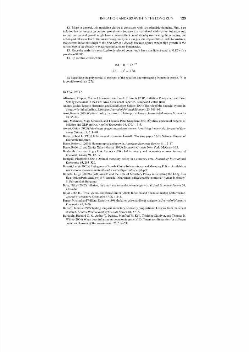
14. To see this, consider that
nA − B = Cn1/3
(nA − B)3 = C3n.
By expanding the polynomial to the right of the equation and subtracting from both terms C 3n, it
is possible to obtain (27).
REFERENCES
Altissimo, Filippo, Michael Ehrmann, and Frank R. Smets (2006) Inflation Persistence and Price
Setting Behaviour in the Euro Area. Occasional Paper 46, European Central Bank.
Andres, Javier, Ignacio Hernando, and David Lopez-Salido (2004) The role of the financial system in
the growth–inflation link. European Journal of Political Economy 20, 941–961.
Aoki, Kosuke (2001) Optimal policy response to relative pricechanges. Journal of Monetary Economics
48, 55–80.
Arai, Mahmood, Mats Kinnwall, and Thoursie Peter Skogman (2004) Cyclical and causal patterns of
inflation and GDP growth. Applied Economics 36, 1705–1715.
Ascari, Guido (2003) Price/wage staggering and persistence: A unifying framework. Journal of Eco-
nomic Surveys 17, 511–40.
Barro, Robert J. (1995) Inflation and Economic Growth. Working paper 5326, National Bureau of
Economic Research.
Barro, Robert J. (2001) Human capital and growth. American Economic Review 91, 12–17.
Barro, Robert J. and Xavier Xala-i-Martin (1995) Economic Growth. New York: McGraw–Hill.
Benhabib, Jess and Roger E.A. Farmer (1994) Indeterminacy and increasing returns. Journal of
Economic Theory 91, 12–17.
Benigno, Pierpaolo (2004) Optimal monetary policy in a currency area. Journal of International
Economics 63, 293–320.Bonatti, Luigi (2002a) Endogenous Growth, Global Indeterminacy and Monetary Policy. Available at
www-econo.economia.unitn.it/new/ricerche/dipartim/paper/p6.pdf.
Bonatti, Luigi (2002b) Soft Growth and the Role of Monetary Policy in Selecting the Long-Run
Equilibrium Path. Quaderni di Ricerca del Dipartimento di Scienze Economiche “Hyman P. Minsky”
6, Universita di Bergamo.
Bose, Niloy (2002) Inflation, the credit market and economic growth. Oxford Economic Papers 54,
412–434.
Boyd, John H., Ross Levine, and Bruce Smith (2001) Inflation and financial market performance.
Journal of Monetary Economics 47, 221–248.
Bruno, Michael and William Easterly (1998) Inflation crises and long-run growth. Journal of Monetary
Economics 41, 3–26.Bullard, James (1999) Testing long-run monetary neutrality propositions: Lessons from the recent
research. Federal Reserve Bank of St.Louis Review 81, 57–77.
Burdekin, Richard C. K., Arthur T. Denzau, Manfred W. Keil, Thitithep Sitthiyot, and Thomas D.
Willet (2004) When does inflation hurt economic growth? Different non-linearities for different
countries. Journal of Macroeconomics 26, 519–532.

8/10/2019 Inflation and Long Run Growth
http://slidepdf.com/reader/full/inflation-and-long-run-growth 33/39
126 ANDREA VAONA
Chambers, Robert G. (1988) Applied Production Analysis. Cambridge, UK: Cambridge University
Press.
Chari, Varadarajan V., Larry E. Jones, and Rodolfo E. Manuelli (1996) Inflation, growth and financial
intermediation. Federal Reserve Bank of St. Louis Review 78, 41–58.
Christopoulos, Dimitri and Efthymios G. Tsionas (2005) Productivity growth and inflation in Europe:
Evidence from panel cointegration tests. Empirical Economics 30, 137–150.
Cooley, Thomas F. and Edward Prescott (1995) Economic growth and business cycles. In Thomas F.
Cooley (ed.), Frontiers of Business Cycles Research, pp. 1–38. Princeton, NJ: Princeton University
Press.
Dotsey, Michael and Pierre D. Sarte (2000) Inflation, uncertainty and growth in a cash-in-advance
economy. Journal of Monetary Economics 45, 631–655.
Fan, Jianqing and Irene Gijbels (1992) Variable bandwidth and local linear regression smoothers.
Annals of Statistics 20, 2008–2036.
Fischer, Stanley (1993) The role of macroeconomic factors in growth. Journal of Monetary Economics
41, 485–512.Funk, Peter and Bettina Kromen (2005) Inflation and Innovation Driven Growth. Working Paper Series
in Economics 16, University of Cologne.
Funk, Peter and Bettina Kromen (2006) Short-term Price Rigidity in an Endogenous Growth Model:
Non-superneutrality and a Non-vertical Long-term Phillips Curve. Working Paper Series in Eco-
nomics 29, University of Cologne.
Ghosh, Atish R. and Steven Phillips (1998) Inflation, Disinflation and Growth. Working paper 98/68,
International Monetary Fund.
Gillman, Max, Mark N. Harris, and Laszlo Matyas (2004) Inflation and growth: Explaining the negative
effect. Empirical Economics 29, 149–167.
Gillman, Max and Michal Kejak (2002) Modelling the effect of inflation: Growth, levels and To-
bin. In David K. Levine and William Zame (eds.), Proceedings of the 2002 North American
Summer Meetings of the Econometric Society: Money. Available at http://www.dklevine.com/
proceedings/money.htm.
Gillman, Max and Michal Kejak (2004) The demand for bank reserves and other monetary aggregates.
Economic Inquiry 42, 518–533.
Gillman, Max and Michal Kejak (2005a) Contrasting models of the effect of inflation on growth.
Journal of Economic Surveys 19, 113–136.
Gillman, Max and Michal Kejak (2005b) Inflation and balanced-path growth with alternative payment
mechanisms. Economic Journal 115, 1–25.
Gillman, Max, Michal Kejak, and Akos Valentinyi (1999) Inflation, Growth, and Credit Services.
Transition Economics Series 13, Institute of Advanced Studies, Vienna.
Gomme, Paul (1993) Money and growth: Revisited. Journal of Monetary Economics 32, 51–77.
Graham, Liam and Dennis Snower (2004) The Real Effects on Money Growth in Dynamic General
Equilibrium. Working paper 412, European Central Bank.
Graham, Liam and Dennis Snower (2008) Hyperbolic discounting and the Phillips curve. Journal of
Money, Credit and Banking 40, 427–448.
Guerrero, Federico (2006) Does inflation cause poor long-term growth performance? Japan and the
World Economy 18, 72–89.
Gylfason, Thorvaldur (1991) Inflation, growth and external debt: A view of the landscape. World
Economy 14, 279–297.
Gylfason, Thorvaldur and Tryggvi T. Herbertsson (2001) Does inflation matter for growth? Japan and
the World Economy 13, 405–428.Gylfason, Thorvaldur and Gylfi Zoega (2006) Natural resources and economic growth: The role of
investment. World Economy 29, 1091–1115.
Haslag, Joseph H. (1998) Monetary policy, banking and growth. Economic Inquiry 36, 439–
450.

8/10/2019 Inflation and Long Run Growth
http://slidepdf.com/reader/full/inflation-and-long-run-growth 34/39
INFLATION AND GROWTH IN THE LONG RUN 127
Haslag, Joseph and Jahyeong Koo (1999) Financial Repression, Financial Development and Economic
Growth. Working paper 99-02, Federal Reserve Bank of Atlanta.
Heijdra, Ben J. and Frederick Van der Ploeg (2002) The Foundations of Modern Macroeconomics.
Oxford, UK: Oxford University Press.
Huang, Kevin X. D. and Zheng Liu (2002) Staggered price-setting, staggered wage-setting, and
business cycle persistence. Journal of Monetary Economics 49, 405–433.
Ireland, Peter (1994) Money and growth: An alternative approach. American Economic Review 55,
1–14.
Jones, Charles I. (1995) Time series tests of endogenous growth models. Quarterly Journal of Eco-
nomics 110, 495–525.
Judson, Ruth and Athanasios Orphanides (1999) Inflation, volatility and growth. International Finance
2, 117–138.
Kahn, Mohsin S. and Semlali A. Senhadji (2001) Threshold effects in the relationship between inflation
and growth. IMF Staff Papers 48, 1–21.
Kim, Sung and Thomas D. Willett (2000) Is the negative correlation between inflation and growthreal? An analysis of the effects of the oil supply shocks. Applied Economics Letters 7, 141–
147.
King, Robert G. and Ross Levine (1993) Finance and growth: Schumpeter might be right. Quarterly
Journal of Economics 108, 717–737.
Levine, Ross (1997) Financial development and economic growth: Views and agenda. Journal of
Economic Literature 35, 688–726.
Li, Qi and Jeffrey S. Racine (2007) Nonparametric Econometrics. Princeton, NJ: Princeton University
Press.
Minford, Patrick and David Peel (2004) Calvo Contracts: A Critique. Discussion Papers 4288, Centre
for Economic Policy Research, London.
Mino, Kazuo and Akihisa Shibata (1995) Monetary policy, overlapping generation, and patterns of
growth. Economica 62, 179–194.
Paal, Beatrix and Bruce Smith (2001) The Sub-Optimality of the Friedman Rule and the Optimum
Quantity of Money. IEHAS Discussion Paper 0113, Institute of Economics, Hungarian Academy of
Sciences, Budapest.
Pagan, Adrian and Aman Ullah (1999) Nonparametric Econometrics. Cambridge, UK: Cambridge
University Press.
Pollin, Robert and Andong Zhu (2006) Inflation and economic growth: A cross-country nonlinear
analysis. Journal of Post-Keynesian Economics 28, 593–614.
Ramsey, James B. (1969) Test for specification errors in classical linear least squares regression
analysis. Journal of the Royal Statistical Society (Series B) 31, 350–371.
Sarel, Michael (1996) Nonlinear effects of inflation on economic growth. IMF Staff Papers 43, 199–
215.
Stockman, Alan C. (1981) Anticipated inflation and the capital stock in a cash-in-advance economy.
Journal of Monetary Economics 8, 387–393.
Temple, Jonathan (2000) Inflation and growth: Stories short and tall. Journal of Economic Surveys 14,
395–426.
Thirlwall, Anthony P. and Christopher A. Barton (1971) Inflation and growth: The international
evidence. Banca Nazionale del Lavoro Quarterly Review 98, 263–275.
Tobin, James (1965) Money and economic growth. Econometrica 33, 671–684.
Vaona, Andrea and Stefano Schiavo (2007) Non-parametric and semiparametric evidence on the long-
run effects of inflation on growth. Economics Letters 94, 452–458.Wang, Ping and Chong K. Yip (1992) Alternative approaches to money and growth. Journal of Money,
Credit and Banking 24, 553–562.
Wolff, Edward N. (2003) What’s behind the rise in profitability in the US in the 1980s and in the
1990s? Cambridge Journal of Economics 27, 479–499.

8/10/2019 Inflation and Long Run Growth
http://slidepdf.com/reader/full/inflation-and-long-run-growth 35/39
128 ANDREA VAONA
Woodford, Michael (1998) Doing without money: Controlling inflation in a post-monetary world.
Review of Economic Dynamics 1, 173–219.
Zhang, Junxi (2000) Inflation and growth: Pecuniary transactions costs and qualitative equivalence.
Journal of Money Credit and Banking 32, 1–12.
APPENDIX A: THE SOLUTION OF THE MODEL
Recall that the macroeconomic model consists of the equations (1), (2), (4)–(6), (9), (12),
(19), and (22)–(25).
Let us first consider the price index (2) in the steady state. Given the absence of price
staggering and due to symmetry, all the firms will charge the same price pf t . So (2) willbecome
pf
p= 1.
By substituting the steady-state price index into (9), it is possible to obtain the result
that in the steady state the marginal cost is the same across all the firms and that in its turn
it can be substituted, together with (8), into the first-order conditions for capital and the
composite labor input to obtain
w
p =θ p − 1
θ pα
y
n , (A.1)
r =θ p − 1
θ p(1 − α)
y
k. (A.2)
Having in mind the equation for capital remuneration, it is possible to obtain the solution
for the steady-state growth rate of the economy by using (22) and (23):
γ = β 1 − δ +θ p − 1
θ p(1 − α)
y
k . (A.3)
Consider the production function in the steady state. The output–capital ratio is given by
y
k= (n)α , (A.4)
where the firm subscript is dropped because all the firms are symmetric.
Substituting (A.4) into (A.3), it is possible to find that in steady state the real growth rate
of the economy depends on the composite labor input:
γ = β
1 − δ +
θ p − 1
θ p (1 − α) nα
. (A.5)
Therefore it is necessary to find the steady-state level of the composite labor input in
order to solve the model. As a first step let us focus on (24). As shown in Graham and
Snower (2004), the labor supply of each cohort can be reduced to the labor supply of cohort

8/10/2019 Inflation and Long Run Growth
http://slidepdf.com/reader/full/inflation-and-long-run-growth 36/39
INFLATION AND GROWTH IN THE LONG RUN 129
zero times a term accounting for money growth:
n0
nj
= µ−θ w j .
Therefore, considering that ρt,t +j = β j , the left-hand side of (24) becomes in the steady
stateN −1j =0
nj,t +j βj = n0
1 − β N µN θ w
1 − βµθ w. (A.6)
As far as the right-hand side of (24) is concerned, divide both the numerator and the
denominator by yt +j :
θ w − 1
θ wς
N −1j =0
βj wj,t
pt +j µj
nj,t +j
ct +j
=θ w − 1
θ wς
N −1j =0
βj wj,t
pt +j µj
nj,t +j yt +j
ct +j
yt +j
. (A.7)
Focusing on the numerator, in steady state, one has
N −1j =1
βj
wj,t
pt +j µj
nj,t +j
yt +j
=
w∗
p
n0
y
N −1j =1
βj µ(θ w −1)j , (A.8)
where w∗ is the steady-state nominal wage rate of cohort zero.
Consider that, due to (11) and to (A.1) one has
wn
py=
N −1j =0
wj,t
µj
nj,t
N
py=
w∗n0
pyN
N −1j =0
µ(θ w −1)j =w∗n0
pyN
1 − µN (θ w −1)
1 − µ(θ w −1) =
θ p − 1
θ pα;
hence
w∗n0
py= N
1 − µ(θ w −1)
1 − µN (θ w −1)
θ p − 1
θ pα.
So it is possible to rewrite (A.8) as follows:
N −1j =1
βj
wj,t
pt +j µj
nj,t +j
y
= N
1 − µ(θ w −1)
1 − µN (θ w −1)
θ p − 1
θ pα
1 − β N µN (θ w −1)
1 − βµ(θ w −1) . (A.9)
Considering the denominator of the right-hand side of (A.7), both consumption and
output are growing at the same rate, so their ratio is a constant in the steady state, and one
can extract it from the sum. Furthermore, given the aggregate budget constraint,
cy
= 1 − iy
. (A.10)
Consider thati
y=
i
k
k
y. (A.11)

8/10/2019 Inflation and Long Run Growth
http://slidepdf.com/reader/full/inflation-and-long-run-growth 37/39
130 ANDREA VAONA
The capital–output ratio can be recovered from the first-order conditions for cost mini-
mization [r = θ p −1
θ p(1 − α)
y
k], whereas the investment–capital ratio can be recovered from
the law of motion of capital:
ik
= γ − 1 + δ.
So by substituting the capital–output ratio and the investment–capital ratio into (A.11)
and taking into consideration (A.2) and (A.3), it is possible to get
i
y=
i
k
k
y= [(1 − δ) β + βr + δ − 1]
θ p − 1
θ p(1 − α)
1
r.
Simplifying and substituting for r by taking into consideration (A.2) and (A.4), it is
possible to perform two further steps:
iy
= (1 − δ) (β − 1) θ p − 1θ p
(1 − α) 1r
+ β θ p − 1θ p
(1 − α)
= (1 − δ) (β − 1) (n)−α + βθ p − 1
θ p(1 − α). (A.12)
Therefore the investment–output ratio depends on labor in efficiency units.
It is time to take stock. By considering (A.6), (A.7), (A.9), (A.10), and (A.12), it is
possible to rewrite (24) as
n0 = 1 − βµ
θ w
1 − β N µN θ w
N 1−µ(θ w −1)
1−
µ
N (θ w −1)
θ p −1
θ p
α1−βN µN (θ w −1)
1−
βµ
(θ w −1) 1 − (1 − δ) (β − 1) (n)−α − β
θ p −1
θ p(1 − α)
θ w − 1θ wς
. (A.13)
It is worth noting that the labor supply of cohort zero depends on the composite labor
input via the investment share of output.
In steady state, the demand for the labor input of cohort zero is equal to
n0 =
w∗
w
−θ w
n, (A.14)
where, assuming (12),w∗
w=
1
N
1 − µN (θ w −1)
1 − µθ w −1
1θ w −1
.
By substituting (A.13) into (A.14), it is possible to obtain
n =
N 1−µ(θ w −1)
1−µN (θ w −1)
θ p −1
θ pα
1−βN µN (θ w −1)
1−βµ(θ w −1)
1 − (1 − δ) (β − 1) (n)−α − βθ p −1
θ p(1 − α)
×
1 − βµθ w
1 − (βµθ w )N
θ w − 1
θ wς 1
N
1 − µN (θ w −1)
1 − µθ w −1
θ wθ w −1
. (A.15)
Simplifying,
n
1 − β
θ p − 1
θ p(1 − α)
− (1 − δ) (β − 1) n1−α (A.16)

8/10/2019 Inflation and Long Run Growth
http://slidepdf.com/reader/full/inflation-and-long-run-growth 38/39
INFLATION AND GROWTH IN THE LONG RUN 131
−
N
1 − µ(θ w −1)
1 − µN (θ w −1)
θ p − 1
θ pα
1 − β N µN (θ w −1)
1 − βµ(θ w −1)
× 1 − βµθ w
1 − (βµθ w )N θ w − 1
θ wς
1N
1 − µN (θ w −1)
1 − µθ w −1
θ wθ w −1
= 0. (A.17)
Suppose, as customary, that α = 2/3:
n
1 − β
θ p − 1
θ p(1 − α)
− (1 − δ) (β − 1) n
13 (A.18)
−
N
1 − µ(θ w −1)
1 − µN (θ w −1)
θ p − 1
θ pα
1 − β N µN (θ w −1)
1 − βµ(θ w −1)
× 1 − βµθ w
1 − (βµθ w )N θ w − 1
θ wς
1N
1 − µN (θ w −1)
1 − µθ w −1
θ wθ
w−1
= 0. (A.19)
Define
A : =
1 −
θ p − 1
θ p(1 − α)
,
C : = (1 − δ) (β − 1),
B : = N 1 − µ(θ w −1)
1 − µN (θ w −1)
θ p − 1
θ pα
1 − β N µN (θ w −1)
1 − βµ(θ w −1) ×
1 − βµθ w
1 − (β µθ w )N
θ w − 1
θ wς
1
N
1 − µN (θ w −1)
1 − µθ w −1
θ wθ w −1
.
As a consequence, the solution for labor in efficiency units is given by the roots of the
following polynomial:14
A3n3 − 3A2Bn2 + (3AB2 − C3)n − B 3 = 0.
With n in mind, one can easily compute γ from (A.5).
APPENDIX B: OPTIMAL MONETARY POLICY
As stated above, welfare is given by
W =
∞
j =0
βj (logCt +j − ς nj t +j ).
Keeping in mind (31) and that Ct +j = ct γ j , it is possible to write for the steady state
W =
∞j =0
βj [logγ j − ς n0µθ w (j ) + log c]. (B.1)

8/10/2019 Inflation and Long Run Growth
http://slidepdf.com/reader/full/inflation-and-long-run-growth 39/39
132 ANDREA VAONA
Given the recursive structure of labor contracts, following Graham and Snower (2004,
p. 23), (B.1) can be written, assuming steady state, as
W =
∞j =0
N −1l=0
β l logγ l −
∞j =0
N −1l=0
β l ς n0µθ w (l) +
∞j =0
N −1l=0
β l logc.
Making explicit the relation of the initial level of consumption with the initial level of
the capital stock, one has
c = y − i,
c = y − (γ − 1 + δ)k,
c = (nα − γ + 1 − δ) k.
The value of k being given by the initial condition, one obtains without loss of generality
W =1
1 − β N logγ
N −1l=0
β l l − ς n0
1
1 − β N
1 − β N µθ w N
1 − βµθ w
+1
1 − β N log (nα − γ + 1 − δ) + const.
Consider that
(1 − β)
N −1l=0
β l l = β + β 2 + · · · + β N −1 + β N − β N N ;
consequentlyN −1j =0
β l l = β1 − β N
(1 − β)2 −
βN N
1 − β
and therefore
W =1
1 − β N β1 − β N
(1 − β)2 −
βN N
1 − β logγ − ς n0
1
1 − β N
1 − β N µθ w N
1 − βµθ w
+1
1 − β N log (nα − γ + 1 − δ).