Inferential Statistics

Coin Flip

• How many heads in a row would it take to convince you the coin is unfair?

• 1?

• 10?

Number of Tosses Approx Probability of All Heads

1 (½)1=.5

2 (½)2=.25

3 (½)3=.125

4 (½)4=.063

5 (½)5=.031

6 (½)6=.016

7 (½)7=.008

8 (½)8=.004

9 (½)9=.002

10 (½)10=.001

100 (½)100=7.88-e31

Not Seen Ad

Seen Ad

Number of Cigarettes smoked per day

Inferential Statistics• To draw inference from a sample about the properties of a

population

• Population distribution: The distribution of a given variable(parameter) for the entire population

• Sample distribution: A sample of size n, is drawn from the

population and the variable’s distribution is called the sample distribution.

• Sampling distribution: This refers to the properties of a particular

test statistic. The sampling distribution draws the distribution of the test statistic if it were calculated from a sample of size n, then resample using n observation to calculate another test statistic. Collect these into the sampling distribution.

• http://onlinestatbook.com/stat_sim/sampling_dist/index.html

• Law of Large Numbers and Central Limit Theorem

• How can we use this information? We can use our knowledge of the sampling distribution of a test statistic, a single realization of that test statistic to infer the probability that it came from a certain population

One Sample T-test of mean

• If the calculate Z statistic is large than the critical value (C.L.) then we reject the null hypothesis, we can also use p-values. That is the exactly probability of drawing a this sample from a population as is hypothesized under the null distribution. If the p-value is large (generally larger than .05 (5%)), we fail to reject the null, if it is small we reject the null.

• Z distribution (standard normal) vs. t-distribution (students t)• The t distribution is used in situations where the population variance is unknown

and the sample size is less than 30.

xS

xZ

Hypothesis testing

• Develop a hypothesis about the population, then ask does the data in our sample support the hypothesized population characteristic.

• Ho: Null hypothesis• Ha: Alternative hypothesis • Significance level. The a critical point where the

probability of realizing this sample when pulled from a population as hypothesized under the under the

• Type I and II Errors (Innocent until proven Guilty)• What if Ho = innocent

• alpha = the nominal size of the test (probability of a type I error)

• Beta = probability of a type II error• 1-beta= the power of a test (ability to reject a false

null)

State of Ho in pop Accept Ho Reject Ho Ho is true Correct Type I error Ho is false Type II error Correct

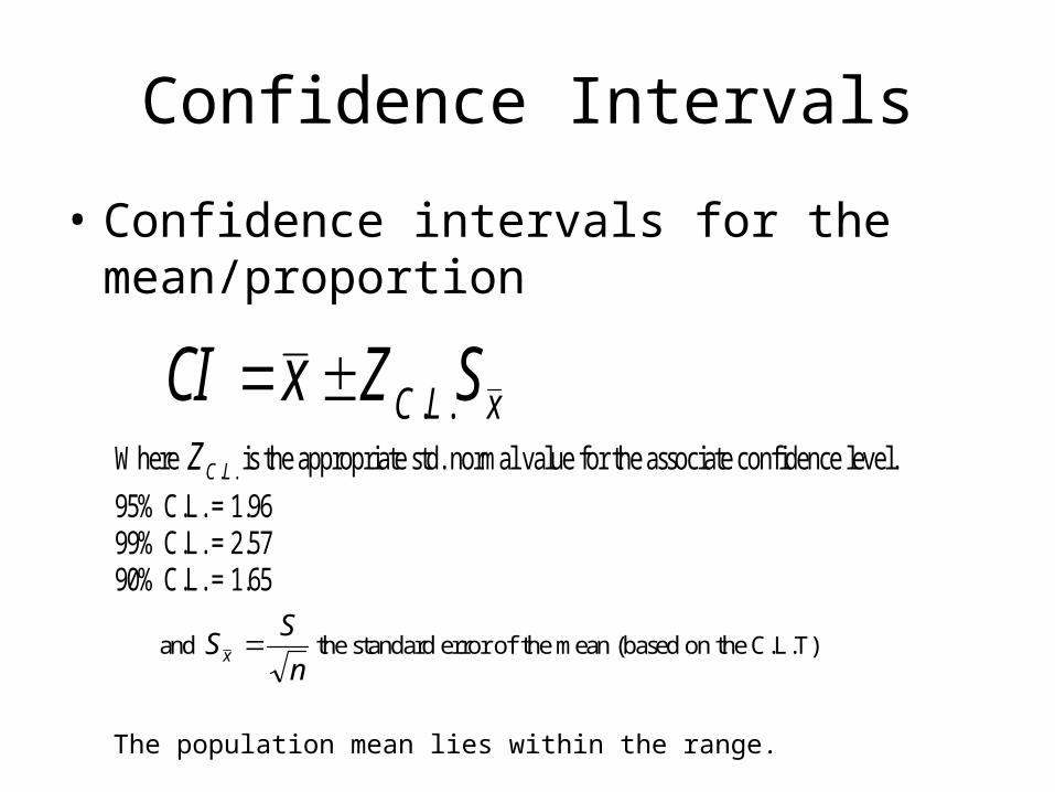
Confidence Intervals

• Confidence intervals for the mean/proportion

xLC SZxCI ..Where ..LCZ is the appropriate std. normal value for the associate confidence level.

95% C.L. = 1.96 99% C.L. = 2.57 90% C.L. = 1.65

and n

SS x the standard error of the mean (based on the C.L.T)

The population mean lies within the range.

Z(T-Test) of proportion

where

pS

pZ

n

ppS p

)1(

• Example:– Males represent 47.9% of the population over the

age of 18.

Ho: 479.

Ha: 479.

Categorical/Categorical

• Crosstabulations (2 way frequency tables, Crosstabs, Bivariate distributions)

Smoke\Gender Male Female Row total

Yes 30 25 55

No 20 25 45

column total 50 50 100

Chi-squared test of independence

• categorical/categorical

• with degrees of freedom (R-1)(C-1) where R = number of rows and C= number of columns

ij

ijij

E

EO 2

2

n

CRE jiij

• χ2=1.01 and the critical value with 1 degree of freedom at the 5% level is 3.84 fail to reject

• H0: The variables are independent, that is to say knowledge of one will not help to predict the outcome of the other

Smoke\Gender Male Female Row total

Yes 30 (27.5) 25 (27.5) 55

No 20 (22.5) 25 (22.5) 45

column total 50 50 100

HOW OFTEN DOES R READ NEWSPAPER * RESPONDENTS SEX Crosstabulation

208 221 429

189.2 239.8 429.0

97 129 226

99.7 126.3 226.0

79 98 177

78.1 98.9 177.0

37 62 99

43.7 55.3 99.0

24 54 78

34.4 43.6 78.0

445 564 1009

445.0 564.0 1009.0

Count

Expected Count

Count

Expected Count

Count

Expected Count

Count

Expected Count

Count

Expected Count

Count

Expected Count

EVERYDAY

FEW TIMES A WEEK

ONCE A WEEK

LESS THAN ONCE WK

NEVER

HOW OFTEN DOESR READNEWSPAPER

Total

MALE FEMALE

RESPONDENTS SEX

Total

Chi-Square Tests

10.933a 4 .027Pearson Chi-SquareValue df

Asymp. Sig.(2-sided)

0 cells (.0%) have expected count less than 5. Theminimum expected count is 34.40.

a.

Categorical/Continuous

• Any statistic that applied to cont. variables done for each category– Mean, median, mode.– Variance, Std dev, skewness, kurtosis

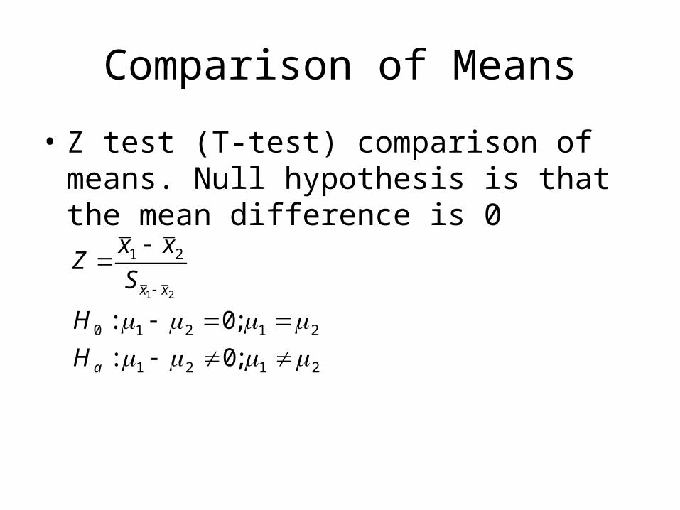
Comparison of Means

• Z test (T-test) comparison of means. Null hypothesis is that the mean difference is 0

21

21

xxS

xxZ

21210 ;0: H

2121 ;0: aH

• Where is the pooled estimate of the standard error of the mean, assuming the underlying population variances are equal.

• Pooled estimate of the standard error (population variances equal)

2

22

1

21

21 n

S

n

SS xx

11

11

21

222

211

nn

SnSnS

21 xxS

Group Statistics

78 46.31 20.512 2.323

931 45.73 17.001 .557

how often r reads news1 Never

0 At Least less thanonce a week

AGE OF RESPONDENTN Mean Std. Deviation

Std. ErrorMean

Independent Samples Test

.286 1007 .775 .583 2.039 -3.418 4.583Equal variancesassumed

AGE OF RESPONDENTt df Sig. (2-tailed)

MeanDifference

Std. ErrorDifference Lower Upper

95% ConfidenceInterval of the

Difference

t-test for Equality of Means

Continuous/Continuous

• Simple Correlation coefficient (Pearson’s product-moment correlation coefficient, Covariance)

• this ranges from +1 to -1

22 )()(

))((

yyxx

yyxxrr

ii

iiyxxy

T-Test of correlation coefficient

r

xy

S

rZ

0

2

1 2

n

rS r

0:0 xyH

0: xyaH

Four sets of data with the same correlation of 0.816