inference for regression find your notes from last week, put # of beers in l1 and bac in l2, then...
TRANSCRIPT
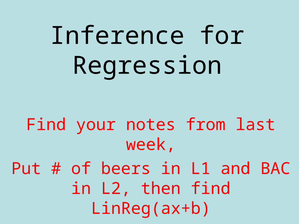
Inference for Regression
Find your notes from last week,Put # of beers in L1 and BAC in
L2, then find LinReg(ax+b)
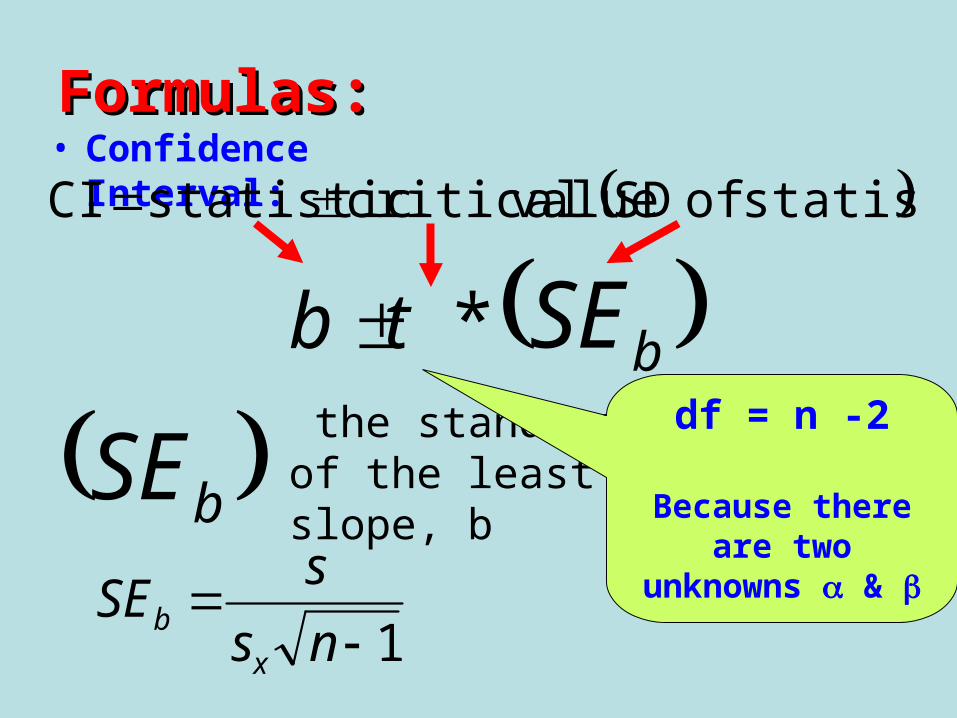
• Confidence Interval:
bSE the standard error of the least squares slope, b
Formulas:Formulas:
b
statistic of SD valuecritical statisticCI
*t bSEdf = n -2
Because there are two unknowns &
1
ns
sSE
x
b

Interpretation:
We are 95% confident that the mean change in BAC per beer is between ___________ and _____________
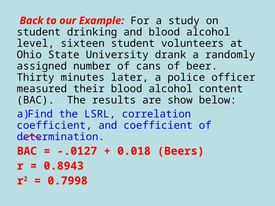
Back to our Example: For a study on student drinking and blood alcohol level, sixteen student volunteers at Ohio State University drank a randomly assigned number of cans of beer. Thirty minutes later, a police officer measured their blood alcohol content (BAC). The results are show below:a)Find the LSRL, correlation coefficient, and coefficient of determination.
BAC = -.0127 + 0.018 (Beers)r = 0.8943r2 = 0.7998

b) Explain the meaning of slope in the context of the problem.
There is approximately 1.8% increase in BAC for every Beer
c) Explain the meaning of the coefficient of determination in context.
Approximately 80% of the variation in BAC can be explained by the regression of BAC on number of Beers drunk.
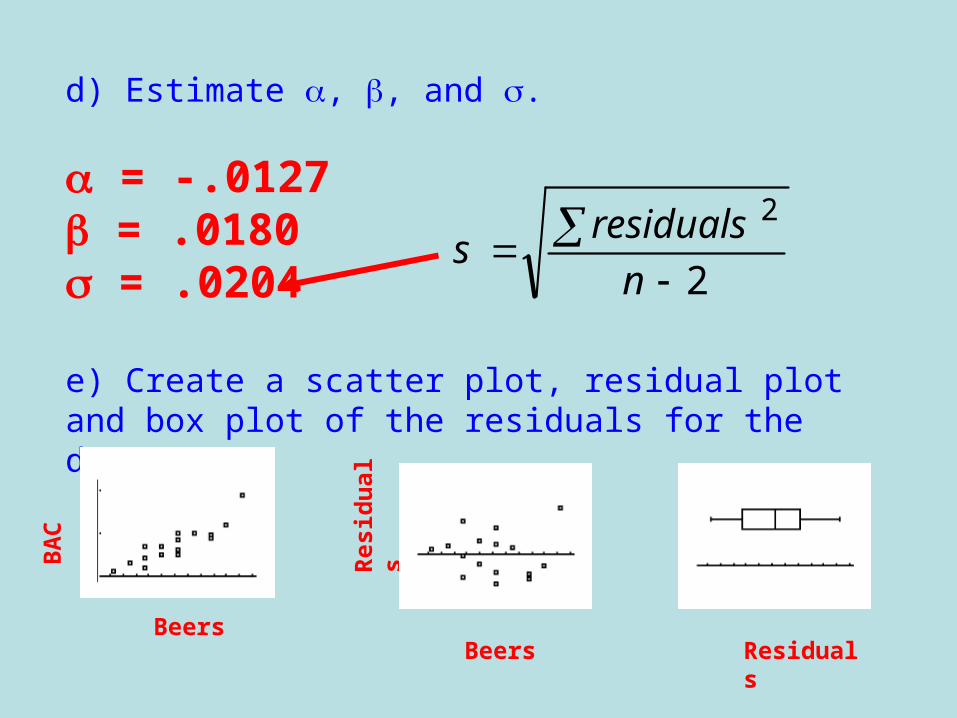
d) Estimate , , and .
= -.0127 = .0180 = .0204
e) Create a scatter plot, residual plot and box plot of the residuals for the data.
2
2
nresiduals
s
Beers
BA
C
Beers
Res
idu
als
Residuals

bSE the standard error of the least squares slope, b

f) Give a 95% confidence interval for the true slope of the LSRL.Assumptions:•Have an SRS of students•Since the residual plot is randomly scattered, BAC and # of beers are linear•Since the points are evenly spaced across the LSRL on the scatterplot, y is approximately equal for all values of BAC•Since the boxplot of residual is approximately symmetrical, the responses are approximately normally distributed.
We are 95% confident that the true slope of the LSRL of weight & body fat is between 0.12 and 0.38.
Be sure to show all graphs!
14
)0231.,0128(.
0024.145.2018.0*
df
SEtb b
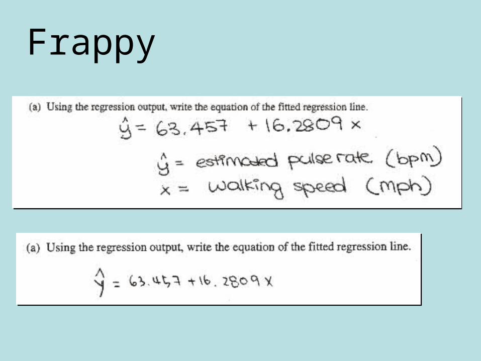
Frappy
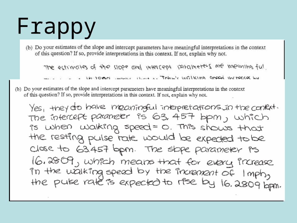
Frappy

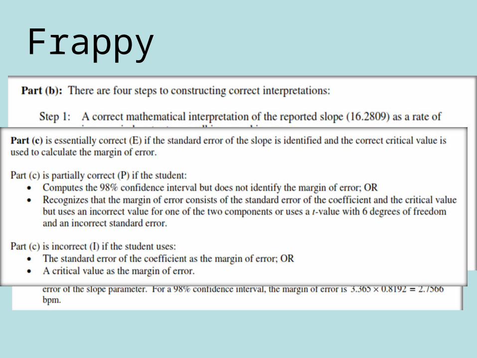
Frappy
Frappy

Formulas:Formulas:• Hypothesis test:
bSE
bt
statistic of SD
parameter - statisticstatisticTest
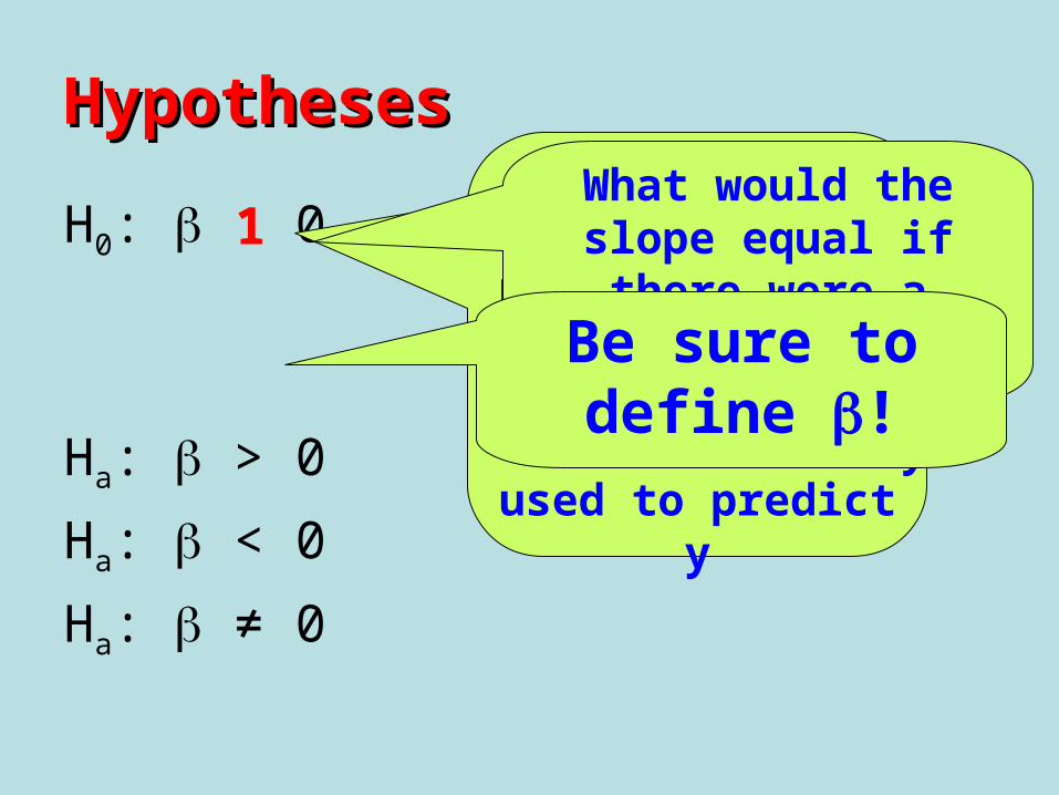
HypothesesHypotheses
H0: = 0
Ha: > 0
Ha: < 0
Ha: ≠ 0
This implies that there is no
relationship between x & y
Or that x should not be used to
predict y
What would the slope equal if there were a perfect relationship
between x & y?
1
Be sure to define !

Median SAT
Expenditure
Grad Rate
1065 7970 49950 6401 331045 6285 37990 6792 49950 4541 22970 7186 38980 7736 391080 6382 521035 7323 531010 6531 411010 6216 38930 7375 371005 7874 451090 6355 571085 6261 48
The data on six-year graduation rate (%), student-related expenditure per full-time student, and median SAT score for a random sample of the primarily undergraduate public universities in the US with enrollments between 10,000 and 20,000 were taken from College Results Online, The Education Trust.
We would like to know if there is
.
For a test of a linear relationship, the null hypothesis is usually expressed as:
In this context, this means
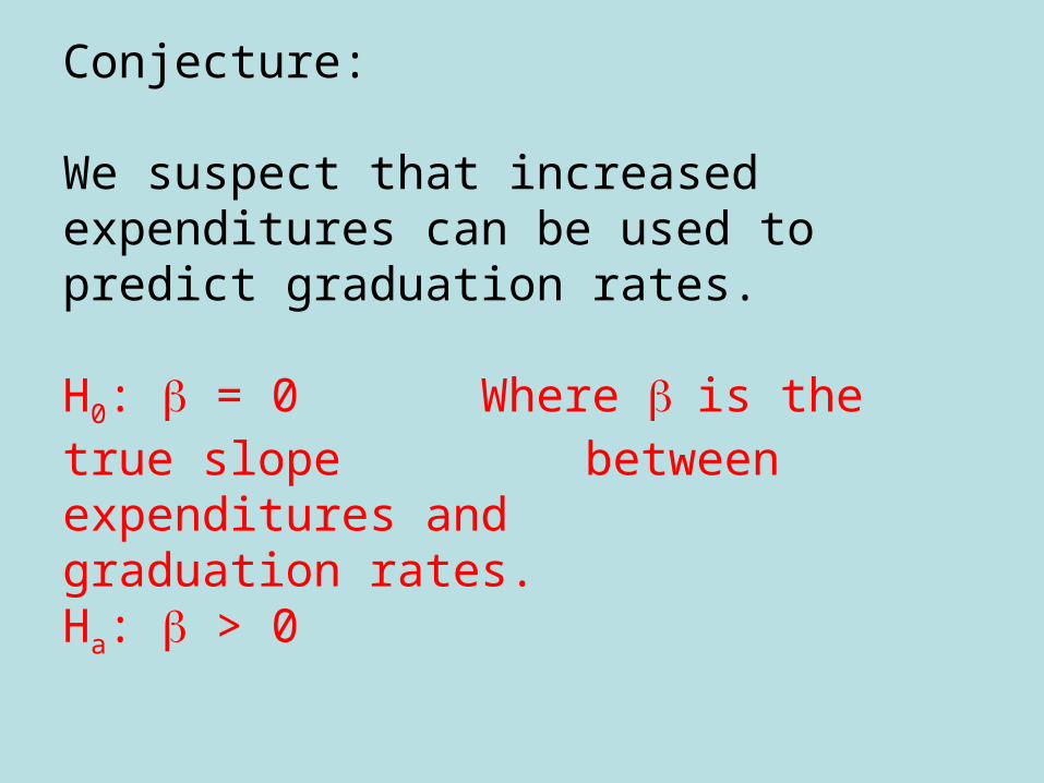
Conjecture:
We suspect that increased expenditures can be used to predict graduation rates.
H0: = 0 Where is the true slope between expenditures and graduation rates.
Ha: > 0
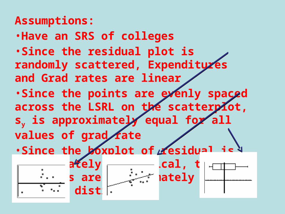
Assumptions:•Have an SRS of colleges•Since the residual plot is randomly scattered, Expenditures and Grad rates are linear•Since the points are evenly spaced across the LSRL on the scatterplot, sy is approximately equal for all values of grad rate•Since the boxplot of residual is approximately symmetrical, the responses are approximately normally distributed.

Test statistic: Linear Regression t-test
05.13
046.
81.100254.
00046.
df
valuep
SE
bt
b
t
bSEb

Since the p-value < a, I reject H0. There is sufficient evidence to suggest that expenditures can be used to predict graduation rate.