UNCC – Sat 5/2/2015

INFERENCE AND REGRESSION

Statistical Inference

Drawing conclusions (“to infer”) about a

population based upon data from a sample.

Two types of inference:

1. Confidence intervals (Estimates)

2. Significance tests (Reject or FTR)

Confidence Intervals

estimate) theoferror ndardvalue)(sta(criticalestimate

Confidence intervals estimate the true value

of the parameter when the parameter is the

true mean , true proportion p, or true slope .

Confidence Intervals

1 2

1-sample t-interval for

2-sample t-interval for

Matched-pairs t-interval

1-proportion z-interval for p

2-proportion z-interval for p1 - p2

t-interval for slope

Interpret the confidence level:

C% of all intervals produced using this method

will capture the true mean (difference in means),

proportion (difference in proportions), or slope.

(Describe the parameter in context!)

Interpret the Confidence Interval:

I am C% confident that the true population

parameter (state it: ICON p, μ, α, β AND WORDS) is captured by the Confidence

Interval [ __ , __ ](insert units and context).

Note: C is the Confidence Level = the %

of the time this process will work successfully

Things to include when answering CI FR questions

Procedure / conditions

Mechanics

– Only the final interval is required if you’ve

correctly identified the procedure.

Interpretation

– Be sure to clarify that you’re estimating the

population parameter (true mean, true proportion)

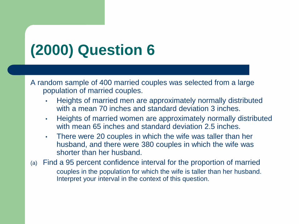
(2000) Question 6

A random sample of 400 married couples was selected from a large population of married couples.

• Heights of married men are approximately normally distributed with a mean 70 inches and standard deviation 3 inches.

• Heights of married women are approximately normally distributed with mean 65 inches and standard deviation 2.5 inches.

• There were 20 couples in which the wife was taller than her husband, and there were 380 couples in which the wife was shorter than her husband.

(a) Find a 95 percent confidence interval for the proportion of married

couples in the population for which the wife is taller than her husband. Interpret your interval in the context of this question.

Solution (2000 – Question 6, part a)

Assumption: SRS stated in problem

Large sample size since

ˆ ˆ20 10 (1 ) 380 10 np n p

Test Name (or formula) / conditions:

1-proportion z-interval

Calculations:

Solution (2000 – Question 6, part a)

Interpret the interval:

I am 95% confident that the true proportion of couples

in which the wife is taller than her husband is captured

by the inteval [.028, .071], based on this sample.

Solution (2000 – Question 6, part a)

Significance Tests

Significance tests provide evidence for some

claim using sample data.

test statistic = estimated value – hypothesized value

standard error of the estimate

Significance Tests

1-sample t-test for

2-sample t-test for

Matched pairs t-test

1-proportion z-test for p

2-proportion z-test for p1 – p2

Chi-square goodness-of-fit test

Chi-square test Chi-square test for homogeneity

Chi-square test for independence/association

t-test for slope

1 2

What is the P-value?

The P-value is the probability of getting the observation in the sample as extreme or even more extreme from value of the parameter by chance alone, assuming that the null hypothesis is true.

If the P-value is small (< alpha = .05), then we reject Ho. P < α REJECT

If the P-value is large (> alpha = .05), then we fail to reject Ho . P ≥ α FAIL to REJECT [FTR]

Know your inference procedures

Helpful web site:

http://www.ltcconline.net/greenl/java/Statistic

s/StatsMatch/StatsMatch.htm

Things to include when answering TOS FR questions

Parameter(s) / hypotheses

Procedure / conditions

Mechanics – Only test statistics (df) and p-value are required if you’ve correctly

stated the procedure.

Conclusion – Statement 1 has to include p → α linkage and decision with

respect to null hypothesis.

– Statement 2 provides context. “There is sufficient evidence to

suggest……..” or “There is insufficient evidence to suggest…….”

(2000) Question 4

Solution (2000) Question 4

Solution (2000) Question 4

Solution (2000) Question 4

Solution (2000) Question 4

Solution (2000) Question 4

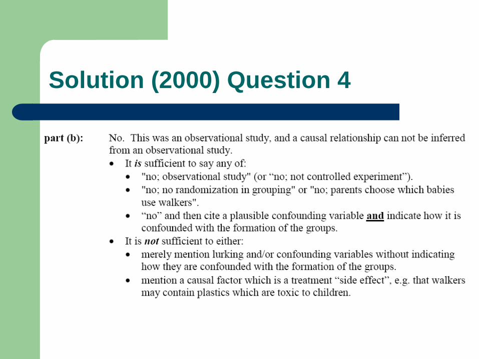
Solution (2000) Question 4

Scoring (2000) Question 4

Scoring (2000) Question 4

(2003) Question 5

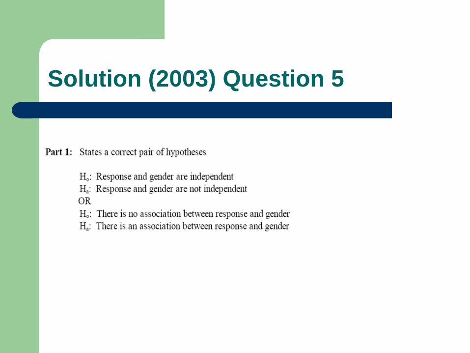
Solution (2003) Question 5

Solution (2003) Question 5

Solution (2003) Question 5

Solution (2003) Question 5

Scoring (2003) Question 5

Type I, Type II Errors & Power

Type I Error:

Ho is true, but we reject Ho & conclude Ha

Type II Error:

Ho is false, but we fail to reject Ho & fail to

conclude Ha.

Power:

the probability of correctly rejecting Ho

Type I, Type II Errors & Power

How to increase power:

Increase alpha (level of significance)

Increase the sample size, n

Decrease variability

Increase the magnitude of the effect (the difference in the hypothesized value of a parameter & its true value

(2003) Question 2

Solution (2003) Question 2

Solution (2003) Question 2

Solution (2003) Question 2

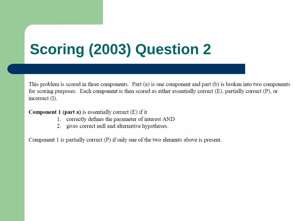
Scoring (2003) Question 2

Scoring (2003) Question 2

Scoring (2003) Question 2

Scoring (2003) Question 2

Reminders on Linear Regression

Quantitative data

Remember that correlation and regression

assess the relationship between 2

QUANTITATIVE variables.

The Linear Regression t-test for Slope tests

for an overall (population) relationship

between 2 QUANTITATIVE variables.

– The Chi-Squ Independence Test checks for a

relationship between 2 CATEGORICAL variables

Explanatory / response variables

The explanatory variable (x) is also known as

the independent variable.

– X explains the data

The response variable (y) is also known as

the dependent variable.

– Y responds to x

– Y is dependent on x

Descriptors for discussing a scatterplot

Form – linear?

Direction – pos/neg

Strength – strong/moderate/weak

Variables

Coefficient of correlation (r)

– Quantifies direction and strength of linear pattern

(scatterplot)

– -1 ≤ r ≤ 1 or │r│ ≤ 1

Coefficient of determination (r2)

– Percent of variation in y that is explained by least-

squares relationship between y and x

Residuals

Residual is difference between predicted y-

value and expected y-value

– y minus y-hat

Residual plot assesses appropriateness of

linear model

– Pattern in residual plot suggests that linear model

is not appropriate

Slope

Slope quantifies the degree to which the

response variable (y) changes for any

corresponding change in the explanatory

variable (x)

– (change in y / change in x)

Interpreting slope

Always cite the actual numbers in the ratio

and the actual variables (context)

– Slope = 2/5

– “Pulse rate (y) increases 2 bpm for each

corresponding increase of 5 lb of body weight (x).”

Y-intercept

Recall that the y-intercept is the constant in

the LSRL, or the value of y when x = 0.

– In the equation: y-hat = -0.25x + 12

-0.25 is the slope

12 is the y-intercept

Interpreting the y-intercept

The y-intercept can often have a very

meaning real-life interpretation.

For the equation

– Pulse rate = 0.12 walking speed + 45

– 45 would be the resting pulse rate (x = 0)

Linear regression t-test for slope β

This TOS assesses, based on the sample LSRL, whether there

is an actual true (population) relationship between 2

quantitative variables.

The test (LinRegTTest) specifically assesses the slope. If the

slope = 0, there is no relationship because y moves without

regard to x. If the slope “significantly” differs from 0, then we

can conclude that there is a relationship.

There is also a Linear Regression T-interval which

accomplishes the same end by estimating the slope of the true

LSRL based on the sample LSRL.

You would need the data to use either of these calculator

functions.

Parameters

The most important unknown population

parameters for the LinReg test are:

– β (capital Greek Beta) for slope, estimated by

sample statistic b

– α (lower case Greek alpha) for y-intercept,

estimated by sample statistic a

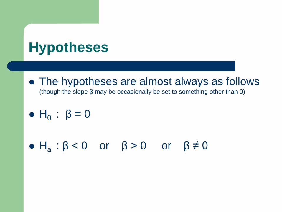
Hypotheses

The hypotheses are almost always as follows (though the slope β may be occasionally be set to something other than 0)

H0 : β = 0

Ha : β < 0 or β > 0 or β ≠ 0

Minitab output

In AP Stats, summary stats are generally

presented in the context of a chart created by

Minitab software.

Most Minitab charts show the LSRL

coefficients, as well as the LinReg test

statistic (t with df) and associated p-value.

Two different measures for standard error

are usually provided, as well.

Example

The regression equation is

Weight = 123 - 5.57 Day

Interpretation: the line intersects y axis at 123 with a slope

of -5.57. That is on the day=0, weight is 123gm and for each

increase in a day, the weight of the soap decreases on the

average by 5.57 grams.

Minitab chart

Predictor Coef SE Coef T P

Constant 123.141 1.382 89.09 0.000

Day -5.5748 0.1068 -52.19 0.000

Note the LSRL coefficients in the Coef. column. The constant will

always be the y-intercept.

Also note the test statistic (t) and p-value in the second (slope) row.

We would certainly be rejecting H0 with such an extreme test statistic

and small (though not equal to exactly 0) p-value

The Minitab output always assumes a 2-sided test (Ha : β ≠ 0)

Standard error of the slopes

0.1068 above is the standard error for the

distribution of all possible slopes. It is

generally referenced with the variable SEb .

Formula for test statistic (t)

The LinReg test statistic follows the same

formula is any other test statistic:

(statistic – parameter) / standard error

– Here, that becomes

– t = (b – β0 ) / SEb

– Since β0 is usually zero, the relationship would be

– t = b / SEb (Note in the example above: -52.19 = -5.5748 / 0.1068)

Good luck!!