1

Comments invited. Preliminary.

Industrialization and Infant Mortality

by Maya Federman and David I. Levine1

On average, infant mortality rates are lower in more industrialized nations, yet industrialization in some nations over time has been associated with worsening health and mortality outcomes. This study examines the effects of growing manufacturing employment on infant mortality across 274 Indonesian districts from 1985 to 1995, a time of rapid industrialization. Compared with cross-national studies we have a larger sample size of regions, more consistent data definitions, and better checks for causality and specification. We can also explore the causal mechanisms underlying our correlations. Overall the results suggest manufacturing employment raised living standards, housing quality, and reduced cooking with wood and coal, both of which helped reduce infant mortality. At the same time, pollution from factories appears quite harmful to infants. The overall effect was slightly higher infant mortality in regions that experienced greater industrialization.

Infant mortality rates today are much lower in industrialized nations than in nations with

low rates of industrialization. At the same time, the great burst of British industrialization in the

second quarter of the nineteenth was associated with “dark Satanic mills,” not improved health.

Death rates did not decline and army recruits actually lost almost an inch (over 2 centimeters) in

height (Steckel and Floud 1997). Similar declines in height accompanied industrialization for at

least a generation in the United States. In contrast, several other nations have industrialized

without a dip in health measures (Steckel and Floud, 1997: 425). A crucial question is whether

industrialization in today’s poor nations is improving or reducing child health.

This study examines the effects of growing manufacturing employment on infant

mortality across 274 Indonesian districts from 1985 to 1995, a time of rapid industrialization.

1 Pizer College and University of California, Berkeley, respectively. We appreciate comments from the

BACPOP seminar, Berkeley. Jules Reinhart and Kok-Hoe Chan provided both data and insights.

2

Compared with cross-national studies we have a larger sample size of regions, more consistent

data definitions, and better checks for causality and specification. We also explore the causal

mechanisms underlying our correlations.2

Just as important as determining the overall correlation is understanding which causal

channels connect industrialization and child health. For example, is industrialization beneficial

because it raises incomes or living standards, harmful due to pollution, or both? If

industrialization motivates urbanization, does the increased crowding help by moving children

closer to health care providers or hurt due to higher exposure to disease? Understanding the

underlying causal channels can help us understand what forms of industrialization are better or

worse for child health and what policies may permit growth in both material standards of living

and richer measures of development.

Links between Industrialization and Child Health

Children are exposed to pathogens in the air they breathe and the water they drink. The

result is almost all children get respiratory illnesses such as colds and digestive problems leading

to diarrhea. For a subset of children these diseases lead to death. Death is more common for

children who are exposed to more pathogens; who have lower resistance due to malnutrition and

lack of immunizations; and who lack health care after becoming sick.

Industrialization can affect the probability of mortality through each of the links in this

chain, exposure to pathogens, resistance, and health care, in various ways. Most obviously,

factories emit pollutants into the air and water. Such emissions are often heavy in poor nations

2 Our study follows the same cross-region methodology of historical studies such as that of Rogers, Brändström and Edvinsson, (2004). As with this study, they find that although early industrialization raised incomes, child mortality rates rose in Swedish region where sawmills were built.

3

such as Indonesia where pollution regulations are only weakly enforced. Air pollution is a major

contributor to the acute respiratory infections (for example, pneumonia) that are the most

common cause of infant mortality (Romieu and others, 2002). Also, just bringing employees

together in a large factory building can increase person-to-person transmission of pathogens.

Working in the opposite direction, industrialization may bring improvements in housing

quality, sanitation, and household pollution, which can improve health outcomes. Similarly,

factories bring jobs and rising incomes to a region which can improve nutrition for both mothers

and children, in turn lowering death rates (Fogel 1994) and can also increase access to health

care,.

Finally, factories are also associated with urbanization. Living near others implies

person-to-person and water-borne pathogens are more easily transmitted. Air pollution from cars

is also worse in cities; Indonesia, for example, uses leaded gas and has limited pollution

regulation. More beneficially, children in cities are usually closer to health care than are those in

rural areas. In addition, cookfires – a major source of indoor air pollution – is less prevalent in

urban areas.

The net result of all these forces is unclear from theory. Thus, we proceed to the data.

The Setting

Indonesia was one of the world’s economic success stories with growth from 1967 to

1997 averaging 4.8 percent per year in real per capita GDP growth. The population living on

one dollar a day dropped from 87.2 million in 1970 to 21.9 million in 1995. Other indicators of

development showed great progress as well: literacy rates rose, immunization rates rose, and

infant mortality declined. (World Bank, 1999).

4

We study 1985 to 1995, a period of rapid industrialization just preceding the 1997-98

financial crisis. Figure 1 shows which districts experienced the greatest growth in manufacturing

employment. Much of the industrialization was concentrated in West Java near the capitol

Jakarta. At the same time, there were concentrations of manufacturing growth spread throughout

the diverse archipelago.

Methods

We compare changes across 274 Indonesian districts from 1985 to 1995 to examine

whether infant health improved faster or slower in districts with faster growth of manufacturing

employment. Our first specification assumes that the mortality of child i in household h in

district d at time t depends on the presence of manufacturing employment in the household

(mfghdt), average manufacturing employment in the district (%mfgdt), features of the child such as

sex and months since birth (Wihdt), features of the household such as its size and demographic

composition (Xhdt), features of the district (Zpt), and a random error (ε):

1) Mortalityhidt = α + β mfgidt + γ %mfgdt + φ Wihdt + δ Xidt + λ Zdt + εidt

We assume the district characteristics Z either observed (zdt) or are constant over time and

across a province (Zp). Thus, we can eliminate all bias from unobserved province characteristics

by adding a vector of province fixed effects (Provincep).3

2) Mortalityhidt = α′ + β′ mfghdt + γ′ %mfgdt + φ W′ihdt + δ X′idt + λ′ zdt

+ λp″ Provincep + ε′hidt .

3 Although our data includes 60,000 births, the limited number of deaths spread out over districts of varying sizes means that there is not sufficient precision to include a complete set of 274 district dummies. Thus, we rely on the province dummies and district characteristics to capture geographic variation.

5

This simple method would be appropriate if people never migrated and if factories

located at random. Neither condition holds in Indonesia, leading to the complications we address

below.

Time-Varying District Characteristics

A potential problem with this specification is that the provincial characteristics may not

be fixed over time and may not be constant for all districts in the province. (Indonesian

provinces are comparable to U.S. states. Provinces average about 10 districts, so typical districts

are a bit larger than typical U.S. counties.) In the worst case, regions change over time in ways

that affect both factory construction and infant mortality. For example, building a main road can

both increase the region’s attractiveness as a site for factories and reduce residents’ costs of

traveling to a health clinic as well as the odds that an infected person has visited a community

recently. If we omit important time-varying district-level covariates Zdt then even with provincial

fixed effects we will bias the estimates of interest, β′ and γ′.

We address this potential problem of omitted factors by controlling for a number of

potential factors likely to affect both infant mortality and industrialization. At the same time,

these factors are potentially endogenous. For example, if manufacturing increases access to

health clinics and health clinics reduce infant mortality, the increased access to health clinics

may moderate the relationship between manufacturing and infant mortality. Thus, we add a

variety of additional potentially endogenous factors at the district and household level to see if

they change the estimated effects of industrial-sector employment in the household and district

(β′ and γ′). We consider district-level measures such as pollution, access to health care, and

sanitation; and household level measures of housing quality, sanitation, and living standards. To

repeat, some of these potentially moderating variables may have an independent effect on

6

manufacturing employment. Thus, the causal interpretation of apparently moderating relations

are discussed with care.

More concerns about causality

A separate set of statistical problems arises due to alternative causality underlying any

effects estimated in equation (2). Two problems are possible: endogenous location of people

(migration) and endogenous location of factories.

In Indonesia, as elsewhere, younger and slightly more educated people migrate toward

factories. Fortunately, we can deal with the issue of migration because we know both the current

district and the district of birth of our sample. We re-estimate our model classifying babies by

the birth district of the mother. This classification ensures the results do not depend on non-

random mothers moving to be near factory jobs. Finally, we rerun analyses dropping all families

that have moved. We also use industrialization in a mother’s birth district as an instrument for

the industrialization of the birth district of her baby. The results below are robust to these

various treatments of migration.

We are concerned that the correlations between household characteristics and

manufacturing employment might not be causal because manufacturing does not select

employees at random. In fact, in Indonesia both male and female manufacturing employees

appear slightly advantaged prior to entering the labor force. Employees in manufacturing had

.75 (for men) to 1 (for women) more year of education than other people their age. (Here the

comparison group included employees, self-employed, and not in the labor force; data from the

1995 Supas.) The above-average education makes it plausible that manufacturing employees

7

also have above-average unobserved skills. If so, the regressions may over-state the causal

effects of household-level manufacturing employment on living standards and child health.4

A final concern is if the arrival of factories is correlated with improved health, but the

causality is reversed. For example, Jeffrey Sachs and Pia Malaney (2003) have argued that the

high mortality and illness due to malaria discourages investment in a region. At the same time,

malaria is a major cause of infant mortality. At least during the time period we studied, infant

mortality was not a useful predictor of factory location. Table 2 presents a district-level

regression that uses district characteristics to predict the growth in manufacturing employment

from 1985 to 1995. Column 1 shows that manufacturing largely located where there were

already factories and in urban regions. When we add infant mortality in 1985 (column 2), the

coefficient is not statistically significant and the point estimate is small. If we drop initial

manufacturing, baseline infant mortality remains unhelpful in predicting factory location (result

not shown).

Data and Measures

We analyze data from a variety of sources collected by Indonesia’s Central Bureau of

Statistics (BPS). Our main data source is the Supas Intercensal Population Survey, which we

supplement with specific measures derived from the Susenas National Socio-Economic Survey,

4 We also examine the earnings of manufacturing employees. This test captures more dimensions of skill than does education, but examines only the third of the work force who are employed in the formal-sector and, thus, report earnings. In addition, wages are also influenced by factors such as rent capture, which can lead manufacturing wages to be higher than justified by human capital alone. Conditioning on a set of 11 age-education interactions, men working in manufacturing had 9 percent (P < .01) higher monthly earnings than men working in other formal-sector jobs (although hourly wages were similar and statistically indistinguishable). The results were similar for women. The results on monthly earnings are reminiscent of results from many nations showing manufacturing jobs tend to be high-paying positions relative to the rest of the economy (e.g., Krueger and Summers 1998). In short, manufacturing appears to hire relatively individuals. (Recall these manufacturing employees in the household are almost entirely male as we do not include the mother)

8

the PODES: Village Potential Statistics, and the Industrial Survey (SI). These data sets are

described in Appendix 1. For all analyses we drop the (now-former) province of East Timor and

the province known during this period as Irian Jaya. We also combine districts that merged or

split between 1985 and 1995 to create a consistent series of districts. In our main analyses, we

link these district-level data from the various datasets with the district and household data from

the 1985 and 1995 Supas (although some surveys are a year off of those dates). Summary

statistics for all variables are presented in Table 1.

Manufacturing employment We measure manufacturing employment with the Supas household survey. We count

someone as a manufacturing employee if he or she works 20 or more hours a week as an

employee or employer in the manufacturing sector. Thus, we eliminate the self-employed and

family workers. At the district level, we measure total manufacturing employment among those

aged 16-60 (male and females in manufacturing) as a share of total potential employment (total

population aged 16-60). From 1985 to 1995, manufacturing as a share of potential employment

increased from 3.3 to 5.3 percent (1.9 to 3.4 percent for women only).5 Because not all adults

work and because we exclude self-employed and family workers, these rates are lower than the

manufacturing share of employment that is often published. Manufacturing employment as a

share of the 1985 full-time economically active population (those unemployed or working over

20 hours per week) grew sharply from 6.3 to 13.1 percent. To control for possible changes in

labor force participation due to industrialization, we focus on the change in manufacturing

employment as a share of total adults, which has a smaller level but the same dramatic growth.

5These rates are higher than those in Table 1 because they use sample weights to estimate the national averages.

9

We also measure manufacturing employment in the household. A household has a

manufacturing worker if any adult age 18-60 other than the mother of the focal child works in

manufacturing. Because we exclude the mothers, this measure is almost entirely men. For

example, 5,7 percent had either a male or a female other than mother work in manufacturing.

Among this group, 5.3 percent had an adult male while only 0.5 percent had an adult female

(other than the mother) in manufacturing. We are concerned about the endogeneity of

manufacturing employment, where (for example) men who were already advantaged are more

likely to have jobs in manufacturing. We test for such sorting below and consider how it may

affect the reported results.

Infant mortality We analyze infant mortality (defined as death of the child before reaching one year of

age). Paralleling the rapid growth in manufacturing, infant mortality declined from 51 to 40 per

thousand births from 1985 to 1995. This decline in only a decade represents very rapid

improvement (although starting from quite high levels). We include only births that took place

within the two years preceding each survey. Respondents to the 1985 Supas reported mortality

for their last two births only (twins count as a single birth); thus, we restrict the Supas 1995 to

the last two births as well.6 Finally, survey questions on births and infant mortality were only

asked of ever-married women age 10-54.

Health Hazards from Factory Emissions An ideal measure of how industrialization affects infants through pollution requires

information on emissions of local factories, how weather and other factors affect the ingestions

6 Because we are already restricting the sample to births in the last two years, few births are lost by restricting the sample to the last two births.

10

of hazardous chemicals by humans, and an understanding of how chemical uptake affects

infants. Each of those pathways is challenging to measure. We proxy the pollution emitted in

each district by the industrial composition of its manufacturing employment. As such we are not

measuring pollution from other industries such as agricultural pesticides and mine tailings. We

combine employment at the 4-digit ISIC level from the SI industrial survey with pollution per

worker per industry constructed as part of the World Bank Industrial Pollution Projection System

(IPPS, see World Bank 2001 and Reinhart 2004; for the toxic intensities see

http://www.worldbank.org/nipr/data/toxint/). Pollutants measured include gases and fine

particulates in the air and amounts of toxic metals released to the land, air and water.

The IPPS data are based on industrial pollution in the US at 1987 levels – a decision

based on the quality and quantity of data in the United States. The IPPS drew from the

population of 200,000 US manufacturing firms spanning approximately 1,500 product

categories, all operating technologies, and hundreds of pollutants. It incorporates a range of risk

factors for human- and eco-toxic effects. These data were combined with economic information

from the 1987 US Census of Manufacturers and the US Environmental Protection Agency’s

(EPA) information on air, water and solid waste emissions in 1987. The IPPS has been used to

analyze data in countries as diverse as the Philippines, Mexico, Thailand, Latvia, and India

(World Bank 2004).

To measure the toxicity of the predicted emissions, we use (the inverse of) 1996

threshold limit values (TLVs). TLV’s are measures of safe toxic exposure levels as determined

by the American Conference of Governmental Industrial Hygienists (ACGIH). They are intended

to measure the time-weighted average concentrations in air that cannot be exceeded without

adverse effects for almost all workers in a normal 40-hour work week. A weight of 1 implies a

11

toxicity equivalent to 1mg of sulfuric acid per cu meter of air. Separate TLVs for the same

chemical in different media were not given. All estimates were constructed using lower bound

pollution intensities, largely due to greater data availability. (This paragraph is based on

http://www.worldbank.org/nipr/data/toxint/). We standardize the predicted pollution index so the

average district has a value of 1 in 1985 by dividing by the 1985 mean.7

Health facilities We analyze data on the number of health facilities per 1000 residents in the district,

including integrated and supplemental health centers maternity houses, and hospitals; and on the

number of doctors per 1000 residents.8

There is substantial evidence that high-quality medical care can improve children’s

outcomes. At the same time, the quality of care in Indonesian health facilities is mixed and it is

not clear that expanding low-quality care has much effect on children’s outcomes. Moreover, the

presence of a medical doctor in a clinic was not helpful in predicting children’s outcomes or the

quality of care (Barber and Gertler, 2002). Thus, the margins we examine – the density of clinics

and of doctors – may not predict infant mortality strongly.

There is also concern about endogenous placement of facilities, where high need may

lead to more facilities (Pitt, Rosenzweig, and Gibbons 1993; Molyneaux and Gertler 2000).

When such causality is common, clinic density can often predict worse outcomes due to the

7 Our pollution index has a number of important limitations. It uses average emissions data from American plants in an industry in 1987 (after serious abatement efforts had begun) to predict Indonesian emissions (where regulations are frequently ignored). Furthermore, the measure ignores the differences among Indonesian plants. Emissions figures translate only approximately into human exposure because our index ignores factors such as the distance between a household and the plant, local weather and geographic conditions, the age of the polluting source, and whether the emission is to the air, land or water. Even when exposure is correct, the medical science translating exposure into biological harm for infants is often uncertain. In spite of these limitations, the pollution intensities have face validity. For example, the calculated industry-specific indices of pollution risk show it is more hazardous to be near a chemical or cement plant than an assembly plant.

8 Results were similar when we analyzed the various types of health facilities separately.

12

decision to place clinics where outcomes are already low. We address this concern partly with

our regional fixed effects and also by testing for endogenous placement explicitly. We find no

evidence that clinics locate in places with high or low infant mortality (Table 4A, columns 7 and

8).

Maternal and household characteristics In most specifications we include a rich set of controls for characteristics of the mother

(education, age and its square as well as dummies for mothers younger than 16 and older than

35, and age at first birth), the child (sex and dummies for months from birth to the survey date)9,

the male head of household (age and its square, education, a dummy if absent) and household

(number of members, age composition, and the proportion of adults that are male). Because

many of these characteristics are potentially endogenous (for example, if industrialization affects

the age of first birth), we rerun specifications including only the predetermined variables of

maternal education and infant sex and age (not shown); results are robust to this alteration.

Results: Industrialization and Infant Mortality

The main results of the paper are presented in Table 3. We present probit estimates of

infant mortality, reported as marginal effects (how the predicted probability of enrollment

changes with a one-unit change of the independent variable). Standard errors are adjusted for the

clustering of observations at the district-year level and all regressions include province fixed

effects.

9 Our sample includes babies who were born in the last 24 months and we examine survival up to age 12 months. Thus, we include dummies for each month since birth of 1 through 12, a dummy for age > 12 months, and a dummy for when only year of birth is present but month of birth is missing (so we can detect infant deaths and survival). Results are unchanged if we drop children with missing month of birth.

13

The share of manufacturing workers in a district has a modest positive coefficient (.10, P

< .05), implying that more manufacturing employment reduces child survival. Five percentage

points more manufacturing (as a share of the potential labor force) raises predicted infant

mortality by 5 deaths per thousand, (a tenth of the mean). Any harm from a district’s

manufacturing is due solely to male manufacturing employment, as the female coefficient is of

the opposite sign and larger (-.14, P < .05). Women are half the potential workforce, so an extra

1% of the potential female workforce working in manufacturing raises the manufacturing

employment rate by 0.5%. The net effect of more female manufacturing workers is close to zero

and not statistically significant.

A manufacturing worker in the household predicts slightly and not statistically

significantly lower mortality -- consistent with the hypothesis that manufacturing pays above-

average wages or with manufacturing employer selecting advantaged employees.

The coefficients on the control variables are generally of the expected sign. For example,

infant mortality declines with both mother’s and male head's education, while children of young

mothers have higher mortality rates. Somewhat surprisingly, holding constant household size,

infants are more likely to survive if the household has a higher share children and a lower share

elderly (the omitted group). With the household controls, the year dummy is not statistically

significant, implying that the 20 percent decline in infant mortality from 1985 to 1995 noted

above can be accounted for by changes in household and maternal characteristics.

Causal channels

An important question is why district level manufacturing (at least among males) appears on net

to increase infant mortality. We examine potential moderating channels that help explain the

observed negative relationship, specifically the increase in pollution associated with rising

14

manufacturing. In addition, we also consider potential channels through which manufacturing

growth may actually improve infant health such as improved sanitation and living conditions. In

Table 4A, we first examine whether growth in manufacturing employment predicts the potential

moderators. In general, results are as expected, with manufacturing growth correlated with rising

pollution improved living conditions and sanitation, and improved access to health care (results

below). In Table 5, we then see how conditioning on these potential moderating channels affects

the estimated relation between industrialization and infant mortality.

While we measure many candidate causal channels, measurement of some elude us. For

example, large-scale manufacturing may bring with it some incorporation of Western science

and values. Child health is likely to improve as people learn the germ theory of disease and

about the benefits of hand washing. Child health is likely to decline if crime rates increase, drug

use becomes more common, or other ills of modern society become more prevalent.

Effects of Pollution We focus first on our index of predicted industrial pollution which should worsen with

increased manufacturing. We then turn to pollution generated by other households in the area

(sanitation, etc.) which may improve if industrialization raises local living standards.

Manufacturing employment growth strongly predicts the growth in the index of predicted

pollution (Table 4A, column 1). If manufacturing doubles as a share of the potential labor force

(from its 1985 mean of 3.4% to 6.8%), the index of predicted pollution harm would is estimated

to rise by 73%. This relationship is partly mechanical as the pollution index is based on

manufacturing employment in each industry times expected pollution in that industry. The

correlation between manufacturing growth and growth in the pollution index is not one to one

because Indonesia shifted toward industries with lower expected pollution per employee from

15

1985 to 1995. (We condition on the square kilometers of the communities in each district to help

capture the dilution effects of larger districts.)

In spite of the coarseness of the index of expected pollution, the measure appears useful

in predicting where manufacturing is harmful. Only those districts whose increased

manufacturing employment was concentrated in those industries associated with higher pollution

in the United States experienced meaningfully higher infant mortality (Table 5, column 2). To

interpret the effect size, consider a district that started with the 1985 mean level of manufacturing

employees distributed in industries with average pollution levels. Now consider what happens if

its manufacturing employment grows to twice the national average and they now work in

industries twice as polluting as average. Such a district would increase pollution from unity

(standardized to be the 1985 mean) to 10. This very large increase in pollution would

correspond to 11 more deaths per thousand live births – undoing the entire average decline from

1985 to 1995. Looking at smaller increases in pollution leads to smaller effects on infant

mortality, but still highly statistically significant.10

At the same time, increasing manufacturing employment in industries that do not predict

the pollution index had a very small and statistically insignificant effect on infant mortality (that

is, the main effect on percent manufacturing in the district is now near zero and not statistically

significant).

Next, we consider three measures of neighbor-generated pollution: cooking fires, lack of

private toilets, and unsafe trash disposal. Improvements in two of the measures are correlated

with the growth of manufacturing: slightly fewer people in the district living in villages where

10 Results were similar, though (as expected) a bit weaker if we used tons of pollution instead of our weighted measure (using TLVs from American Conference of Governmental Industrial Hygienists index of expected harm per gram of each chemical) to create our index of expected pollution harm.

16

most people use firewood (Table 4a, column 2), and slightly more people living in communities

where most people use a private toilet. The third measure, the share of the district who lives in

villages where most people have places to put their trash (as opposed to dumping it in the river or

other disposal method such as burning) is uncorrelated with manufacturing changes (Table 4a,

column 4). Thus, we do not test its role as a mediating variable. When we condition on the two

candidate community pollution measures, having more people in communities where most

people use a private toilet predicts slightly but statistically significantly lower infant mortality:

10 percentage points more people in such communities lowers infant mortality by 1 death per

thousand live births. When conditioning on community firewood and private toilet use, the

coefficient on district manufacturing gains statistical significance and rises from .10 to .15,

although the increase is not statistically significant.

Industrialization and urbanization Industrialization and urbanization are intertwined processes. As shown in Table 4A,

column 6, growth in manufacturing is strongly correlated with growth in urbanization in a

district, with causality almost surely running both directions. Factories bring migrants to

urbanize a region and factories locate where potential workers are already concentrated; that is,

in urban areas. Thus, any apparent effects of factories may partly be picking up the related

phenomenon of urbanization.

We can bound the total effect of industrialization by removing the control for

urbanization (Table 5, column 4). In that specification the coefficient on manufacturing declines

slightly from .099 to .088 (difference not significant). Thus, it does not appear that much of the

link between manufacturing and infant mortality runs through the correlation of factories and

urbanization.

17

Health facilities We first examine whether growth in manufacturing predicted more clinics or doctors.

We then explore whether the growth in clinics was a factor moderating the relationship between

manufacturing growth and infant mortality. Manufacturing growth had a small but usually

positive relationship with the number of health care facilities per capita. A 5 percentage point

increase in total manufacturing (a large change) predicts .02 more doctors per thousand residents

(about a sixth of the 1985 mean, Table 4A, column 6, P < .10), and .07 total health care facilities

per thousand (a third of the 1985 mean, column 8, P < .05).

Though associated with increased manufacturing in the district, the number of medical

doctors and the number of health facilities per thousand residents in a district does not correlate

with infant mortality (Table 5, column 5). These result contrasts with the more usual result that

health facilities are useful (e.g., Frankenberg 1995). Because our measures of health care

facilities are not correlated with infant mortality, including them in the regression has no effect

on the estimated coefficients on industrialization.11

There is a concern that facilities are built where needs are greatest (leading to a false

negative correlation). At the same time, we have province fixed effects so that is unlikely to be

the entire story. In addition, in our data 1985 infant mortality rates are not useful in predicting

the growth of clinics (Table 4A, columns 6 and 7). While it always remains possible that new

clinics were built in response to shocks to infant health, that possibility appears unlikely given

lags in building and given Indonesia’s budget-driven allocation of most health facilities. Thus, it

is unlikely our results are strongly biased by endogenous program placement. Instead, our zero

result may be due to the modest quality level of many Indonesian health facilities (Barber and

11 Breaking down health care facilities into more detailed types does not change the result.

18

Gertler 2002) or may be due to our inability to match clinic building to specific communities (as

was done by Frankenberg [1995] in her study of Indonesian clinic building during the mid-

1980s).

Access to health care also increases when road quality increases. In results not shown,

the effects of industrialization on infant health were not mediated by rising road quality.

Household Level Living Standards, Sanitation and Cooking Pollution One possible benefit of increased industrialization is a higher standard of living at the

household level. Industrialization both employs people directly and increases employment in

related business services and among some suppliers too small to be picked up as manufacturing

by our definitions. Higher incomes for these employed people can in turn increase employment

for those who provide locally made goods and services. To the extent that migration or capital

mobility takes time to equilibrate wages in different regions, industrialization in a local labor

market will push up average incomes and living standards. Along with more nutrition and health

care may come better sanitation and less pollution from cooking with wood or coal. We have

proxies for each of these channels. Thus, we first examine which of these potential moderators

are correlated with manufacturing; we next turn to see which correlate with infant survival.

Table 4B examines whether measures district and household manufacturing predicts

these household level characteristics: specifically, housing quality12, having a private toilet, high-

quality water source (pipe, pump or well, not a common surface source), electricity, cooking

pollution (from wood or charcoal), the log of house size, and an asset measure (ownership of a

TV, radio, stove and bicycle).

12 Our index of housing quality is an index from 0 to 3 of the number of strong floor, roof and floor, where a strong floor is marble, ceramic, tile or brick (as opposed to wood, bamboo, earth, or other), strong walls are brick or wood (as opposed to bamboo or other), and a strong roof is concrete wood or tile (as opposed to asbestos, corrugated zinc, leaves, or other).

19

Housing quality, better sanitation (both having a private toilet and higher quality water

source), electricity, and the number of consumer durables (the count of TV, radio, stove and

bicycle) are all higher when a district has more manufacturing (Table 4b, columns 1-5).

Similarly, the use of wood or charcoal as a cooking fuel (which maybe be associated with greater

indoor pollution) is less common (column 6). These results are consistent with such rising

incomes. At the same, houses are a bit smaller in high-manufacturing districts (column 7),

consistent with high population density and property values near factories.

Because manufacturing generally predicts increases in these measures of material well-

being, if we adjust for this improved house quality and the other measures of material well-

being, we expect that manufacturing should predict even higher infant mortality than in our

baseline (Table 3, column 2, reproduced as Table 5, column 1). That is, in fact, what we find.

Manufacturing in a district is more strongly correlated with higher infant mortality when

controlling for living standards than when not; the coefficient rises by a third from .10 to .13

(although the change is not statistically significant, Table 5, column 6).

As expected, cooking with a polluting heat source (wood or charcoal) predicts higher

infant mortality. The increase is 5 deaths per thousand live births, or over 10 percent of the 1995

mean – a large effect.13 Similarly, a private toilet has a large beneficial effect as does a high-

quality housing structure. Several of the measures related to prosperity such as floor size, the

number of durable assets and a high-quality source of drinking water (pipe, pump or well) do not

predict lower infant mortality by statistically significant amounts. Together, these results suggest

that the measures with direct health effects (private toilet and low-smoke cooking) more than

living standards in general matter for improvements in infant mortality.

13 Cooking fires might have an even stronger effect if we could break down those fires that occur indoors, as indoor fires are associated with the greatest health risks.

20

Most of these improvements in living conditions are also associated with having a

manufacturing worker in the household. Having a manufacturing worker in the household

predicts higher assets and house quality fairly consistently as well as predicting lower use of

wood or charcoal (Table 4B).

Overall, when conditioning on these household characteristics the effects of

manufacturing employment in the region rises from .10 to .13 (P < .05, comparing Table 5

column 1 to column 6). The increase is economically meaningful although not statistically

significant. Surprisingly, the effects of a manufacturing worker in the household remains small

and not significant. Thus, it appears likely that the benefits of manufacturing that come in part

from rising living standards (and less cooking over wood or coal, presumably due in part to

urbanization) throughout the nearby region – not just among manufacturing employees

themselves. As with the results on pollution from industry, manufacturing appears to be

important due to its effects on pollution from households.

Finally, we expected that community-level poverty might lead to higher infant mortality.

Manufacturing in a district weakly predicts higher consumption among the poor (as measured by

the 20th percentile of per capita consumption expenditures, measured from the SUSENAS

survey, table 4A, column 5). Surprisingly, a low level of consumption among the bottom fifth

does not predict higher infant mortality (Table 5, column 7). Conditioning on this measure of

21

poverty does not affect the estimated coefficient on manufacturing. Results were similar

conditioning on median per capita consumption in each district (results not shown).14

Summary of results on potential causal channels

As pollution is harmful and living standards helpful to children, the overall effect of

manufacturing on infant mortality is near where we started with all controls (Table 5, col. 8).

The residual harm is plausibly due to measurement error on pollution – an area of active

research.

The Role of Direct Foreign Investment

Critics of globalization have emphasized the incentives global firms have to shift high-

emissions plants to poor nations. On the one hand, the economic logic of shifting highly

regulated production to a region with weaker regulations is clear. On the other hand, there is no

14 We ran several robustness checks with no change in results. We ran the regressions

adding one characteristic at a time. Results are qualitatively similar as when mediating channels

were entered separately.

Also, in our baseline specification we included maternal and household characteristics

that, as noted above, may be endogenous. In fact, changes in household composition are not

strongly related to manufacturing growth (Federman and Levine, 2005). Nevertheless, as a

robustness check, we reran the main results dropping all of these variables except maternal

education (which is largely predetermined) and infant sex and age. Results were very similar to

those presented in the text (results not shown).

22

evidence that avoiding regulation is a measurable determinant of direct foreign investment

(Levinson 2000). In addition, even if DFI plants are dirtier than the average plant in rich nations,

they may still be cleaner than the average plant in their sector in poor nations. This lower level

of pollution can be due to use of more modern technologies, better management that avoids

costly leaks, higher visibility with regulators and the public poor nations, and stronger concern

for reputation in wealthy nations. Consistent with these stories, Eskeland and Harrison (1997)

find that in four developing nations, DFI factories use less energy and use somewhat cleaner

fuels than do locally owned plants in those industries. DFI might also help reduce infant

mortality if foreign-owned plants paid above-average wages. Lipsey and Sjoholm, 2001, find

such higher wages to be the case in Indonesia). Nevertheless, in some cases opponents of

foreign investment have emphasized how foreign owned firms in China often ignore labor laws

and can actually reduce wages and worsen labor conditions (see the many case studies in

Kernaghan 1998).

We do not have plant-level data on emissions in Indonesia. The typical (that is, median)

foreign-owned plant is in an industry with higher/lower {to be calculated xx} than the average

domestically owned plant. This calculation ignores any higher or lower pollution that foreign-

owned plants might produce compared to others in their industry. To the extent foreign-owned

plants are more visible to regulators, visible to the Indonesian public, and more responsive to bad

press from their home market, it is plausible they pollute less than otherwise similar locally-

owned plants. To the extent foreign-owned plants are more capital intensive, they may create

more output per employee. The corresponding increase in inputs may lead to more pollution per

employee (even if not to more pollution per unit of output). Grant and Jones (2004) find no

23

pollution gap among foreign- versus domestically-owned plants in the United States; evidence

from less industrialized nations is lacking.

In fact, the presence of foreign-owned firms in a district does not have a statistically

detectable effect on the harm that manufacturing employment does not infants (Table 7, column

1). The district DFI share interacted with district percent manufacturing is also not statistically

significant, although its coefficient (.112, SE = .75) is large. Taking the point estimate literally

implies that increasing the share of the potential labor force working in foreign owned plants by

2 percentage points (= raising employment by 4 % of the actual labor force, a very large

increase) would increase infant mortality by almost a fourth (11 deaths per thousand). Although

very imprecise and (to repeat) not statistically significant, this coefficient is large enough to

suggest grounds for concern.

At the same time, it is important to recall that even if foreign-owned manufacturing has

no excess effect on infant health relative to other manufacturing, the main effect of

manufacturing employment on infant mortality is negative. Thus, even an estimate of zero on

the interaction is still consistent with foreign-owned plants being at least as hazardous as

domestically-owned plants of similar employment.

Conclusions

Summary

Infant mortality rates are slightly higher in regions with many manufacturing employees.

This relationship appears related solely to growth in male manufacturing employment.

Moreover, any harm is due to manufacturing employment in a region, not employment in the

household.

24

This correlation may not be causal if factories locate in unhealthy regions or if

disadvantaged parents move to be near factory jobs. In fact, factory location is uncorrelated with

infant mortality rates in this sample. Moreover, migrants are slightly advantaged and adjusting

for migration with an instrumental variable technique leaves the basic results unchanged. The

household correlations are statistically insignificant and also more suspect because

manufacturing employees appear slightly advantaged in the labor market prior to their

manufacturing job.

Much of the apparent harm factories do to infants appears related to factory pollution. At

the same time, children benefit from the rising living standards associated with factories. Of

particular importance are measures correlated with air pollution (lower firewood use at home and

in the district) and person-created water pollution (more use of private toilets at home and in a

district). Urbanization, in contrast, has little relationship with the manufacturing-mortality nexus.

Cautions

Much of our understanding of industrialization’s effects on health comes from the vast

and detailed historical research on British industrialization. At the same time, careful scholars

have noted that such studies are just case studies of one industrialization – albeit the first. Two

centuries later, it is worth examining more recent examples of industrialization to see how

children fare. At the same time, it is important to recall that this, like its British predecessors, is

just a case study of one example of industrialization. It is possible that children in China or

Mexico (to take two recent large cases) may have had quite different experiences than those in

Indonesia as there are many possible reasons for industrializations to differ.

For example, Amartya Sen has noted that female employment sometimes increases

female empowerment within the household (2001). If so, female employment may shift

25

resources toward female goals, and these goals are frequently child-focused. At the same time,

we would expect the importance of employment on female power to be lower in Indonesia than,

for example, in much of India as women in Indonesia have traditionally had more authority than

women in South Asian (Kevane and Levine 2002).

Indonesia during this period had a highly centralized tax and expenditures policy. Thus,

a district that successfully industrialized and, thus, raised more tax revenue did not necessarily

have substantially more to spend on health care or clean water. In nations with more

decentralized fiscal policies, including Indonesia in recent years, the public health benefits of

industrialization that increases tax revenue is likely to be larger. At the same time, if

jurisdictions expend almost all of their potential revenue bidding for manufacturing plants, then

total expenditures on health care and clean water can decline nation-wide.

Finally, because we lack longitudinal data, we cannot examine the effects of

manufacturing employment on the children of manufacturing employees. Factory jobs can

increase exposure to chemicals, reduce the length of breastfeeding, raise incomes, and have

many other important effects for good and ill. Future research should examine that important

question.

Implications Economists frequently define “industrialization” as “development” when we speak of

“less industrialized” or “less developed” nations. At the same time, development is a much

broader concept than building new factories. In a companion analysis, we find that increased

industrialization in Indonesia was associated with modestly higher school enrollments and

reduced work among young teens. Less optimistically, here we find that industrialization

predicts slower declines in infant mortality.

26

We are able to decompose the effects of industrialization into two clear pieces: rising

living standards help and industrial pollution hurts. In the broader debate on economic

development, the refrain is often heard to industrialize first, and worry about pollution later. Our

results give some cause for concern, and suggest it is important to look for cost-effective

regulations at the regional level and to encourage rising incomes to be channeled into cleaner

cooking methods and waste disposal at the household and community level.

27

Figure 1: Industrial development in Indonesia, 1985-199515

15 Percentage change in the proportion of manufacturing workers 1985 to 1995 among population aged 16-

60 years, district averages, SUPAS. Light gray denotes the bottom third of districts in terms of percentage change in

industrialization, gray denotes the middle third of districts, and dark gray denotes the top third of districts. The

white areas on the map – East Timor and Irian Jaya – are excluded from the analysis.

28

Data Appendix

Supas: The Intercensal Population Surveys

We examine the 1985 and 1995 Intercensal Population Surveys (Supas) each of which

has responses from roughly 240,000 households. Households are interviewed to obtain

information regarding issues such as education, fertility, mortality and migration.

The Supas sample was selected to be representative for each of Indonesia’s roughly 300

districts. The survey over-samples smaller districts to increase precision.

Susenas: National Socio-Economic Survey

The National Socio-Economic Survey (Susenas) is an annually repeated cross section. It

surveyed between 20,000 and 50,000 households per year in the mid-1980s and approximately

200,000 households per year by the mid-1990s. Sampling rules follow those of the Supas.

Susenas surveys the head of the household on the general welfare of each household

member in areas such as school enrollment, health, and mortality. Susenas has information on

mortality in the previous year.

PODES: Village Potential Statistics

The Village Potential Statistics (PODES) survey provides information about the

characteristics of villages or urban neighborhood. We analyze the 1986 and 1996 surveys.

Roughly 65,000 village heads fill out the survey about their village.

For most measures we average the village-level responses to the district level, typically

weighting by population.

29

We computed the high schools for youth 13-15, high schools for those 16-18) per

thousand youth in tha tage range (as in Duflo, 2001).

The Industrial Survey

The Industrial Survey is an annual census of employers with over 20 employees. We use

employment and the count of factories from the Industrial Survey to measure the intensity of

industry in a district.

The Indonesia Family Life Survey (IFLS)

The IFLS is a representative sample of 83 percent of the population on Indonesia as of

late 1993, covering 13 of Indonesia’s 27 provinces (Frankenberg and Thomas 2001). The

smallest provinces and politically unstable regions – such as Irian Jaya and the former East

Timor – were not sampled. Within households different members were interviewed according to

various selection criteria to ensure adequate numbers of older respondents. We use both cross-

sectional and retrospective information from the 1997 survey on over 7224 households

distributed across several hundred communities.

30

Appendix for the Referee: The Role of Migration

The main goal of this paper is to understand the causal channels that may link

manufacturing employment and child survival. Before we turn to that question we address issues

of migration. A concern with the causal interpretation of these results is that the migration can

affect the mix of people near factories. For example, if poor rural peasants migrate to

shantytowns near factories, then the presence of factories may predict high infant mortality but

not cause the poor health. Instead, the children of the poor peasants might have suffered poor

health even if the peasants had stayed as landless laborers in the rural region. Alternatively, if

young and healthy people migrate, factory regions might show below-average infant mortality

solely due to who moves there.

To examine the importance of non-random migration we first show that migrants are not,

on average, notably advantaged or disadvantaged (Appendix 2, table A1).

We next use an instrumental variable strategy, using a manufacturing employment in a

mother’s birth district as an instrument for the manufacturing intensity in her current district.

The two are highly correlated (see table A2, the first stage of the instrumental variable

estimation).

The reduced form is presented in Table A3, column 3, where the manufacturing intensity

in a mother’s birth district is used instead of her current district to predict infant mortality.

Results are almost identical to the probit results using current manufacturing rates.

The IV results switch to two stage least squares (Table A3, column 4). The instrumental

variable results show an effect of male manufacturing slightly higher than OLS results (in the

appendix) and the probit with no correction for migration. The change in coefficients is not

statistically significant.

31

Appendix table 2: First Stage of the Instrumental Variable Regression on Migration

dprobit current dist

ols current dist

iv current dist

dprobit birth dist

District % mfg of all workers 0.104 0.09 0.158 [1.71]* [1.24] [1.67]* District % mfg of fem workers -0.143 -0.13 -0.193 [1.84]* [1.59] [1.83]* District % mfg of all workers in mother’s birth district 0.124 [2.19]** District % mfg of female workers in mother’s birth district -0.15 [2.06]** Male mfg worker in HH -0.005 -0.009 -0.01 -0.005 [1.83]* [2.74]*** [2.87]*** [1.91]* Female mfg worker in HH 0.017 0.005 0.005 0.017

[1.53] [0.33] [0.32] [1.53]

Instruments for column 3 are District % mfg of all workers and for female workers in

mother’s birth district.

Next version will have OLS on using mother’s birth district as well as the F-test and

incremental R2 of mom’s birth district %mfg and %female mfg.

1 2 3 4

1995 cross section

Baseline: Pooled 1985

and 1995

Reduced form: Mother coded in birth

district

Birth district %mfg

instruments for current

Probit Probit Probit IV-2SLS 0.134 0.088 0.092 0.124

District % mfg of all workers [2.24]** [1.72]* [1.76]* [2.19]** -0.148 -0.129 -0.107 -0.15

District % mfg of female workers [1.92]* [1.92]* [1.60] [2.06]** -0.004 -0.003 -0.004 -0.005

Male mfg worker in household [1.50] [1.34] [1.57] [1.91]* 0.003 0.01 0.008 0.017 Female (other than mother) mfg worker

in household [0.36] [1.18] [0.97] [1.53] Additional controls for household, mother, child and year Yes Yes Yes Yes

32

Province * urban rural No Yes Yes Yes

31221

62559

62595

62559

Note: Probit effect sizes are changes in probabilities when the independent variable changes one unit. Standard errors are clustered at the level of the 274 districts * urban or rural * year. In column 4: District % mfg of all workers and for female workers from the mother’s birth district are used as instruments for current District % mfg of all workers and for female workers. Note: Next version will be IV-Probit.

33

References

Barber, Sarah L. and Paul J. Gertler, “Child Health and the Quality of Medical Care,” working paper, University of California, Berkeley, 2002. [http://faculty.haas.berkeley.edu/gertler/working_papers/02.28.02_childheight.pdf]

Rogers, John, Anders Brändström and Sören Edvinsson, “Paying for Progress: Child Mortality during early Industrialization im Sweden,” paper presented at the Social Science History Association, Chicago IL, 2004.

Easterly, William. 1999. “Life during Growth: International Evidence on Quality of Life and Per Capita Income,” World Bank WPS 2110 (May).

Grant, Don and Andrew W. Jones, “Do Foreign-Owned Plants Pollute More? New Evidence from the U.S. EPA Toxics Release Inventory,” Society and Natural Resources, 17:171–179, 2004

Eskeland, Gunnar and Ann Harrison, “Moving to Greener Pastures? Multinationals and the Pollution Haven Hypothesis,” World Bank, January 1997.

Feridhanusetyawan, Tubagus , Haryo Aswicahyono and Ari A. Perdana, “The Male-Female Wage Differentials in Indonesia,” Centre for Strategic and International Studies, Jakarta, Indonesia, Economics Working Paper Series with number WPE059, 2001. [http://www.csis.or.id/working_paper_file/21/wpe059.pdf]

Frankenberg, Elizabeth, “The effects of access to health care on infant mortality in Indonesia,” Health Transition Review 5, 1995, 143 – 163.

Kernaghan, Charles, Made in China, National Labor Committee, New York, 1998. Krueger, Alan and Summers, Lawrence, "Efficiency Wages and the Inter-Industry Wage Structure", Econometrica,

1988, HB 139 + OP + JSTOR. http://links.jstor.org/sici?sici=0012-9682%28198803%2956%3A2%3C259%3AEWATIW%3E2.0.CO%3B2-5

Levinson, Arek, “The Missing Pollution Haven Effect: Examining some Common Explanations,” Review of International Economics, 15, 4, 2002: 343-64.

Lipsey, Robert E., and Fredrik Sjoholm, “Foreign Direct Investment and Wages in Indonesian Manufacturing” NBER working paper 8299, 2001. [http://www.nber.org/papers/w8299.pdf]

Miguel, Ted, Paul Gertler and David I. Levine. 2002. “Did Industrialization Destroy Social Capital in Indonesia?” mimeo, University of California, Berkeley.

Molyneaux, J., Gertler, P.J., 2001. The Impact of Targeted Family Planning Programs in Indonesia. Population and Development Review. 26 (suppl 1) 61-85.

Pitt, M., M. Rosenzweig, and D. Gibbons. 1993. The determinants and consequences of the placement of government programs in Indonesia. World Bank Economic Review 7, 3: 319-348.

Reinhart, Jules, work in progress, 2004. Sachs, Jeffrey, and Pia Malaney “The economic and social burden of malaria” Nature Nature, Vol. 415, no. 6872,

Feb. 7, 2002. [http://www.nature.com/cgi-taf/DynaPage.taf?file=/nature/journal/v415/n6872/full/415680a_fs.html]

Romieu I, Samet JM, Smith KR, Bruce N. "Outdoor air pollution and acute respiratory infections among children in developing countries." Journal of Occupational and Environmental Medicine. 2002 Jul; 44(7): 640-9.

Sen, Amartya, “The Many Faces of Gender Inequality,” The New Republic September 17, 2001. [Accessed from http://www.ksg.harvard.edu/gei/Text/Sen-Pubs/Sen_many_faces_of_gender_inequality.pdf, Jan. 18, 2005

Steckel, Richard, and Roderick Floud, eds. 1997. Health and Welfare during Industrialization. National Bureau of Economic Research Project Report. Chicago: University of Chicago Press.

World Bank. 1999. “Indonesia and Poverty” in Social Policy and Governance in the East Asia and Pacific Region, [http://www.worldbank.org/poverty/eacrisis/countries/indon/pov1.htm]

World Bank, New Ideas in Pollution Regulation web page (2001). “Using IPPS: The Industrial Pollution Projection System” http://www.worldbank.org/nipr/ipps/index.htm

World Bank, (2004) “Industrial Pollution Modeling & Data” web page [http://www.worldbank.org/nipr/polmod.htm] accessed February 23, 2004.

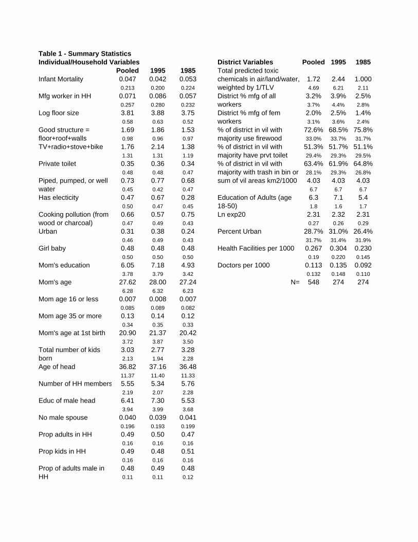
Table 1 - Summary StatisticsIndividual/Household Variables District Variables Pooled 1995 1985

Pooled 1995 1985Infant Mortality 0.047 0.042 0.053 1.72 2.44 1.000

0.213 0.200 0.224 4.69 6.21 2.11Mfg worker in HH 0.071 0.086 0.057 3.2% 3.9% 2.5%

0.257 0.280 0.232 3.7% 4.4% 2.8%Log floor size 3.81 3.88 3.75 2.0% 2.5% 1.4%

0.58 0.63 0.52 3.1% 3.6% 2.4%1.69 1.86 1.53 72.6% 68.5% 75.8%0.98 0.96 0.97 33.0% 33.7% 31.7%

TV+radio+stove+bike 1.76 2.14 1.38 51.3% 51.7% 51.1%1.31 1.31 1.19 29.4% 29.3% 29.5%

Private toilet 0.35 0.36 0.34 63.4% 61.9% 64.8%0.48 0.48 0.47 28.1% 29.3% 26.8%0.73 0.77 0.68 sum of vil areas km2/1000 4.03 4.03 4.030.45 0.42 0.47 6.7 6.7 6.7

Has electicity 0.47 0.67 0.28 6.3 7.1 5.40.50 0.47 0.45 1.8 1.6 1.70.66 0.57 0.75 Ln exp20 2.31 2.32 2.310.47 0.49 0.43 0.27 0.26 0.29

Urban 0.31 0.38 0.24 Percent Urban 28.7% 31.0% 26.4%0.46 0.49 0.43 31.7% 31.4% 31.9%

Girl baby 0.48 0.48 0.48 Health Facilities per 1000 0.267 0.304 0.2300.50 0.50 0.50 0.19 0.220 0.145

Mom's education 6.05 7.18 4.93 Doctors per 1000 0.113 0.135 0.0923.78 3.79 3.42 0.132 0.148 0.110

Mom's age 27.62 28.00 27.24 N= 548 274 2746.28 6.32 6.23

Mom age 16 or less 0.007 0.008 0.0070.085 0.089 0.082

Mom age 35 or more 0.13 0.14 0.120.34 0.35 0.33

Mom's age at 1st birth 20.90 21.37 20.423.72 3.87 3.503.03 2.77 3.282.13 1.94 2.28

Age of head 36.82 37.16 36.4811.37 11.40 11.33

Number of HH members 5.55 5.34 5.762.19 2.07 2.28

Educ of male head 6.41 7.30 5.533.94 3.99 3.68

No male spouse 0.040 0.039 0.0410.196 0.193 0.199

Prop adults in HH 0.49 0.50 0.470.16 0.16 0.16

Prop kids in HH 0.49 0.48 0.510.16 0.16 0.160.48 0.49 0.480.11 0.11 0.12

Prop of adults male in HH

% of district in vil with majority use firewood% of district in vil with majority have prvt toilet% of district in vil with majority with trash in bin or

Total number of kids born

Total predicted toxic chemicals in air/land/water, weighted by 1/TLV

Good structure = floor+roof+walls

Piped, pumped, or well water

Cooking pollution (from wood or charcoal)

Education of Adults (age 18-50)

District % mfg of all workersDistrict % mfg of fem workers

Table 2: Predicting Growth in District % mfg of potential workers(1) (2) (3)

District % mfg of potentia 0.252 0.252 0.230[4.32]*** [4.34]*** [3.93]***

Percent Urban in 1985 0.005 0.004 0.011[1.12] [0.80] [1.41]

District Area (km2) -0.0004 -0.0004 -0.0004[1.41] [1.38] [1.44]

Infant Mortality in 1985 -0.054 -0.045[1.22] [0.98]

Education of Adults (age 18-50) 0.0098[2.19]**

Education of Adults (-mean) squared -0.0009[2.28]**

Constant 0.008 0.012 -0.015[0.90] [1.20] [0.86]

Observations 274 274 274R-squared 0.31 0.32 0.33Notes: OLS regressions with province fixed effects. T-

Table 3 - Predicting Infant Mortality(1) (2)

District % mfg of all workers 0.10179[1.97]**

District % mfg of fem workers -0.13147[2.04]**

Mfg worker in HH -0.00289[1.13]

Urban -0.00272 -0.00294[1.60] [1.68]*

sum of vil areas km2 -0.00005 -0.00005[0.44] [0.40]

Education of Adults (age 1 -0.0024 -0.00238[4.28]*** [4.16]***

Education of Adults (-mea -0.00014 -0.00014[0.97] [0.94]

Girl baby -0.00482 -0.00481[4.09]*** [4.09]***

Mom's education -0.00115 -0.00115[4.85]*** [4.83]***

Mom's age 0.00127 0.00127[4.01]*** [4.04]***

Mom's age (-mean) squar -0.00007 -0.00007[4.58]*** [4.58]***

Mom age 16 or less 0.14586 0.14526[8.25]*** [8.24]***

Mom age 35 or more -0.00801 -0.00803[2.95]*** [2.96]***

Mom's age at 1st birth -0.00139 -0.00139[4.15]*** [4.16]***

Total number of kids born 0.01406 0.01402[15.43]*** [15.39]***

Age of head 0.0005 0.0005[5.10]*** [5.09]***

Age of head (-mean) squa -0.00003 -0.00003[5.55]*** [5.52]***

Number of HH members -0.00723 -0.0072[12.56]*** [12.52]***

Educ of male head -0.00103 -0.00102[4.62]*** [4.58]***

No male spouse 0.00523 0.00542[1.30] [1.35]

Prop adults in HH 0.02644 0.02673[2.56]** [2.59]***

Prop kids in HH -0.20619 -0.20596[18.11]*** [18.11]***

Prop of adults male in HH -0.00119 -0.00108[0.19] [0.17]

Year is 1995 -0.00373 -0.00379[2.37]** [2.39]**

Observations 62595 62595Notes: Dprobits with province fixed effects and dummies for months elapsed between birth and the survey as described in the text. Z-statistics robust to clustering at the district*year level. * significant at 10%; ** significant at 5%; *** significant at 1%

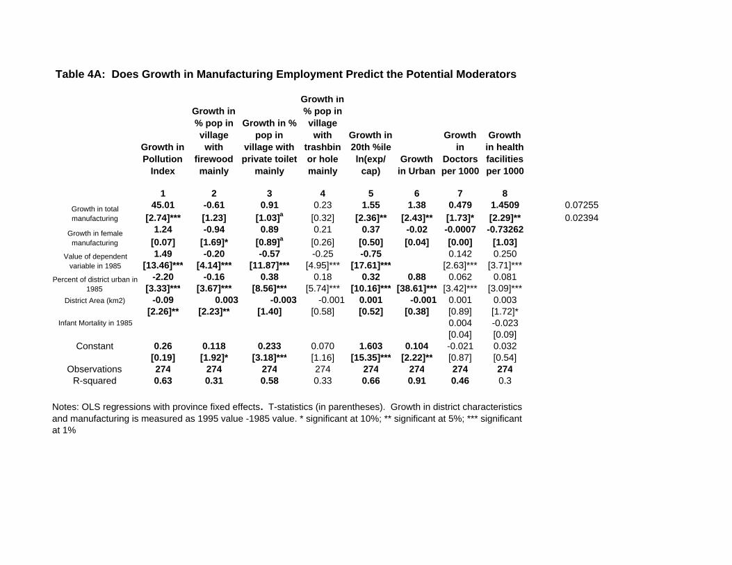
Table 4A: Does Growth in Manufacturing Employment Predict the Potential Moderators

Growth in Pollution

Index

Growth in % pop in village with

firewood mainly

Growth in % pop in

village with private toilet

mainly

Growth in % pop in village with

trashbin or hole mainly

Growth in 20th %ile ln(exp/

cap) Growth

in Urban

Growth in

Doctors per 1000

Growth in health facilities per 1000

1 2 3 4 5 6 7 845.01 -0.61 0.91 0.23 1.55 1.38 0.479 1.4509 0.07255

[2.74]*** [1.23] [1.03]a [0.32] [2.36]** [2.43]** [1.73]* [2.29]** 0.023941.24 -0.94 0.89 0.21 0.37 -0.02 -0.0007 -0.73262

[0.07] [1.69]* [0.89]a [0.26] [0.50] [0.04] [0.00] [1.03]1.49 -0.20 -0.57 -0.25 -0.75 0.142 0.250

[13.46]*** [4.14]*** [11.87]*** [4.95]*** [17.61]*** [2.63]*** [3.71]***-2.20 -0.16 0.38 0.18 0.32 0.88 0.062 0.081

[3.33]*** [3.67]*** [8.56]*** [5.74]*** [10.16]*** [38.61]*** [3.42]*** [3.09]***District Area (km2) -0.09 0.003 -0.003 -0.001 0.001 -0.001 0.001 0.003

[2.26]** [2.23]** [1.40] [0.58] [0.52] [0.38] [0.89] [1.72]*Infant Mortality in 1985 0.004 -0.023

[0.04] [0.09]Constant 0.26 0.118 0.233 0.070 1.603 0.104 -0.021 0.032

[0.19] [1.92]* [3.18]*** [1.16] [15.35]*** [2.22]** [0.87] [0.54]Observations 274 274 274 274 274 274 274 274

R-squared 0.63 0.31 0.58 0.33 0.66 0.91 0.46 0.3

Growth in total manufacturing

Growth in female manufacturing

Value of dependent variable in 1985

Percent of district urban in 1985

Notes: OLS regressions with province fixed effects. T-statistics (in parentheses). Growth in district characteristics and manufacturing is measured as 1995 value -1985 value. * significant at 10%; ** significant at 5%; *** significant at 1%

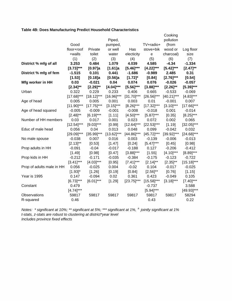
Table 4B: Does Manufacturing Predict Household Characteristics

Good floor+roof

+wallsPrivate toilet

Piped, pumped, or well water

Has electicity

TV+radio+stove+bik

e

Cooking pollution

(from wood or

charcoal)Log floor

size(1) (2) (3) (4) (5) (6) (7)

District % mfg of all 3.253 0.484 1.079 4.039 4.585 -4.34 -1.334[3.73]*** [0.97]a [1.61]a [5.46]*** [4.22]*** [5.42]*** [2.47]**

District % mfg of fem -1.515 0.101 0.441 -1.686 -0.989 2.485 0.31[1.53] [0.18]a [0.56]a [1.72]* [0.84] [2.76]*** [0.54]

Mfg worker in HH 0.03 -0.021 0.04 0.074 0.076 -0.026 -0.057[2.34]** [2.29]** [4.04]*** [5.56]*** [3.88]*** [2.26]** [5.39]***

Urban 0.322 0.229 0.233 0.406 0.665 -0.533 -0.069[17.68]*** [18.12]*** [16.96]*** [31.70]*** [26.56]*** [40.21]*** [4.83]***

Age of head 0.005 0.005 0.001 0.003 0.01 -0.001 0.007[11.90]*** [17.75]*** [3.15]*** [8.26]*** [17.32]*** [3.10]*** [17.66]***

Age of head squared -0.005 -0.009 -0.001 -0.008 -0.018 0.001 -0.014[2.48]** [6.19]*** [1.11] [4.50]*** [5.87]*** [0.35] [8.25]***

Number of HH members 0.03 0.017 0.001 0.023 0.072 0.002 0.065[12.54]*** [9.03]*** [0.99] [12.64]*** [22.53]*** [1.19] [32.05]***

Educ of male head 0.056 0.04 0.013 0.048 0.099 -0.042 0.032[29.09]*** [35.99]*** [13.62]*** [44.86]*** [45.72]*** [39.92]*** [24.68]***

No male spouse -0.038 0.007 0.016 0.003 -0.139 -0.006 -0.013[2.13]** [0.53] [1.47] [0.24] [5.47]*** [0.45] [0.98]

Prop adults in HH -0.091 -0.04 -0.017 -0.188 0.127 -0.206 -0.412[1.49] [0.98] [0.47] [3.88]*** [1.55] [4.10]*** [8.89]***

Prop kids in HH -0.212 -0.171 -0.035 -0.384 -0.175 -0.123 -0.722[3.41]*** [4.03]*** [0.95] [7.41]*** [2.14]** [2.35]** [15.18]***

Prop of adults male in HH 0.056 -0.025 0.004 -0.02 0.104 -0.017 -0.025[1.93]* [1.26] [0.19] [0.84] [2.56]** [0.76] [1.15]

Year is 1995 0.147 -0.094 0.02 0.361 0.423 -0.049 0.105[6.73]*** [6.01]*** [1.29] [23.75]*** [15.58]*** [3.18]*** [7.40]***

Constant 0.479 -0.737 3.588[4.74]*** [5.94]*** [49.93]***

Observations 59817 59817 59817 59817 59817 59817 58294R-squared 0.46 0.43 0.22

t-stats, z-stats are robust to clustering at district*year levelIncludes province fixed effects

Notes: * significant at 10%; ** significant at 5%; *** significant at 1%, a jointly significant at 1%

Table 5 - adding potential causal/mediating channels(1) (2) (3) (4) (5) (6) (7) (8)

District % mfg of all workers 0.102 0.052 0.152 0.090 0.112 0.133 0.095 0.108[1.97]** [0.95] [2.77]*** [1.78]* [2.10]** [2.58]*** [1.78]* [1.92]*

District % mfg of fem workers -0.131 -0.118 -0.151 -0.123 -0.134 -0.150 -0.127 -0.144[2.04]** [1.74]* [2.32]** [1.93]* [2.08]** [2.38]** [1.97]** [2.11]**

Mfg worker in HH -0.003 -0.003 -0.003 -0.003 -0.003 -0.003 -0.003 -0.003[1.13] [1.13] [1.16] [1.18] [1.16] [1.04] [1.12] [1.08]

Urban -0.003 -0.003 -0.001 -0.002 0.001 -0.003 0.002[1.68]* [1.61] [0.82] [1.31] [0.42] [1.73]* [0.86]

0.0004 0.0004[2.51]** [2.76]***

0.0068 0.0076[1.44] [1.33]

-0.0089 -0.0076[2.56]** [2.23]**

Health facilities per 1000 0.008 0.0043[1.20] [0.68]

Doctors per 1000 -0.019 0.0014[1.64] [0.11]

Log floor size -0.0002 -0.0002[0.13] [0.14]

Good structure = floor+roof+walls -0.0023 -0.0023[2.63]*** [2.66]***

TV+radio+stove+bike -0.0002 -0.0002[0.37] [0.26]

Private toilet -0.0031 -0.0024[2.12]** [1.65]*

Piped, pumped, or well water 0.0013 0.0015[0.87] [1.07]

Has electicity -0.0016 -0.0014[1.00] [0.84]

Cooking pollution (from wood or charcoal) 0.0057 0.0053[3.15]*** [2.86]***

lnexp20 0.0026 0.0055[0.64] [1.37]

Observations 62595 62595 62595 62595 62595 62595 62595 62595

Dprobits with prov fixed effectsz-stats robust to cluster at dist*yearIncludes province fixed effects, fixed effects for months baby has been alive, and all controls in Table 3Column (1) replicates results from Table 3, column 2* significant at 10%; ** significant at 5%; *** significant at 1%

Total predicted toxic chemicals in air/land/water, weighted by 1/TLV % of district in vil with majority use firewood% of district in vil with majority have prvt toilet

Table 6: DFI as a predictor of infant mortality(1) (2) (3)

District % mfg of all workers 0.102 0.103 0.089[1.97]** [1.95]* [1.67]*

District % mfg of fem workers -0.131 -0.130 -0.128[2.04]** [2.01]** [1.95]*

Mfg worker in HH -0.003 -0.003 -0.003[1.13] [1.12] [1.11]

Urban -0.003 -0.002 -0.002[1.68]* [1.39] [1.37]

% of mfg. that is DFI 0.001 -0.003[0.27] [0.33]

% of mfg. that is DFI * %mfg. 0.112[0.75]

Observations 62595 59123 59123Notes:Dprobits z-stats robust to cluster at dist*yearIncludes province fixed effects, fixed effects for months baby has been alive, and all controls in Table 3* significant at 10%; ** significant at 5%; *** significant at 1%