inf-geo 3310/4310: imaging in seismology · inf-geo 3310/4310 - imaging in seismology v. maupin,...
TRANSCRIPT
INF-GEO 3310/4310 - Imaging in seismology
V. Maupin, Nov 2007 1
1
INF-GEO 3310/4310:Imaging in seismology
Valérie MaupinDepartment of Geosciences
University of Oslo, Norway.

INF-GEO 3310/4310 - Imaging in seismology
V. Maupin, Nov 2007 2
2
The Earth internal structure seen by seismology
What is imaging in seismology?Most of the imaging studies concern imaging the interior of the structure of the Earth. By analyzing the arrival times of waves, we map the 3-D distribution of the P and S-wave velocities and the locations in discontinuities (interfaces between layers). Variations in wave velocity inside the Earth are primarily related to variations in composition and to variations in temperature: warm material are softer and the waves travel more slowly there. In the mantle, the composition is believed to be rather homogeneous and the dominant effect is the one related to temperature. Here you see the main structure of the Earth: the mantle in green with its lowermost layer in blue. And the iron-rich core with its liquid outer core in light red and solid inner core in dark red. The crust at the surface is a thin layer of 10 to 70km which you do not see at the scale of this figure. Imaging in seismology covers all scales from the scale of seismics (a few km) to the whole Earth. But since the arrival time of the waves at a given seismological station depends on the origin time and location of the earthquake, on which we have no control, we cannot do tomographic studies without locating the earthquakes in space and time. This has therefore to be done first. In addition, if we know the structure well enough, we can use the seismograms to analyze the rupture itself along the fault plane where the earthquake has occurred. These source studies are not as numerous as the structure studies but they are very important because they contribute to our understanding of the physics of earthquake rupture and will hopefully lead to methods for predicting earthquakes.

INF-GEO 3310/4310 - Imaging in seismology
V. Maupin, Nov 2007 3
3
Differences with seismics:
Fewer sources and no control onsource location.Fewer stations.Few earthquakes and few stations: nosingle imaging method based on a transformation: iterative procedurebased on improving initial guesses

INF-GEO 3310/4310 - Imaging in seismology
V. Maupin, Nov 2007 4
4
What is an earthquake?Imaging: early studies and the meanstructure of the EarthP-wave tomographyNormal mode tomographySource location and time-reversal

INF-GEO 3310/4310 - Imaging in seismology
V. Maupin, Nov 2007 5
5
Location of earthquakes
First, for the non-geophysicists, I will explain shortly what earthquakes are.
This shows the distribution of earthquakes of magnitude at least 5 during most of the last century. You see that they are not distributed randomly, but follow basically some lines along the surface of the Earth. In red you have the shallow earthquakes and in green and blue the deep ones. The deepest earthquakes are located at about 700km depth.
The earthquakes occur along the boundaries of the tectonic plates and arise from sudden relaxation of the stresses which occur when two plates are trying to move past each other.

INF-GEO 3310/4310 - Imaging in seismology
V. Maupin, Nov 2007 6
6
Example of an earthquake
This example illustrates how earthquakes occur at subduction zones. South of Indonesia, the Indian Ocean plate is moving northwards and diving below the Eurasian plate, which is relatively fixed at the Earth surface. Due to friction at the contact between the two plates, the Eurasian plate is gradually bent at its south end by the movement of the Indian plate. When the forces associated with the bending get larger than a given threshold, the Eurasian plate suddenly slips on the Indian plate and gets back to its undeformed position. This occurs over basically a few seconds, up to a few minutes for the very large earthquakes, and this movement generates vibrations in the whole Earth, which are then registered by seismometers.

INF-GEO 3310/4310 - Imaging in seismology
V. Maupin, Nov 2007 7
7
The elastic rebound
Forces associated with plate motion act onplates, but friction inhibits motion until a givenstress is reached. Then, slip occurs suddenly.
Not only subduction zone earthquakes, but basically all earthquakes occur as the sudden release of accumulated tectonic stresses.

INF-GEO 3310/4310 - Imaging in seismology
V. Maupin, Nov 2007 8
8
Plate Boundaries
Earthquakes occur therefore mostly where we have tectonic plate boundaries- Where two plates slide past one another- Where two plates run into one another - convergent boundary (subduction or continental collision)- Where plates move away from one another - divergent boundary

INF-GEO 3310/4310 - Imaging in seismology
V. Maupin, Nov 2007 9
9
Earthquakes in subduction zones
In subduction zones, the earthquakes occur down to 700km depth. In other parts of the Earth, they are confined to the first 100km.
INF-GEO 3310/4310 - Imaging in seismology
V. Maupin, Nov 2007 10
10
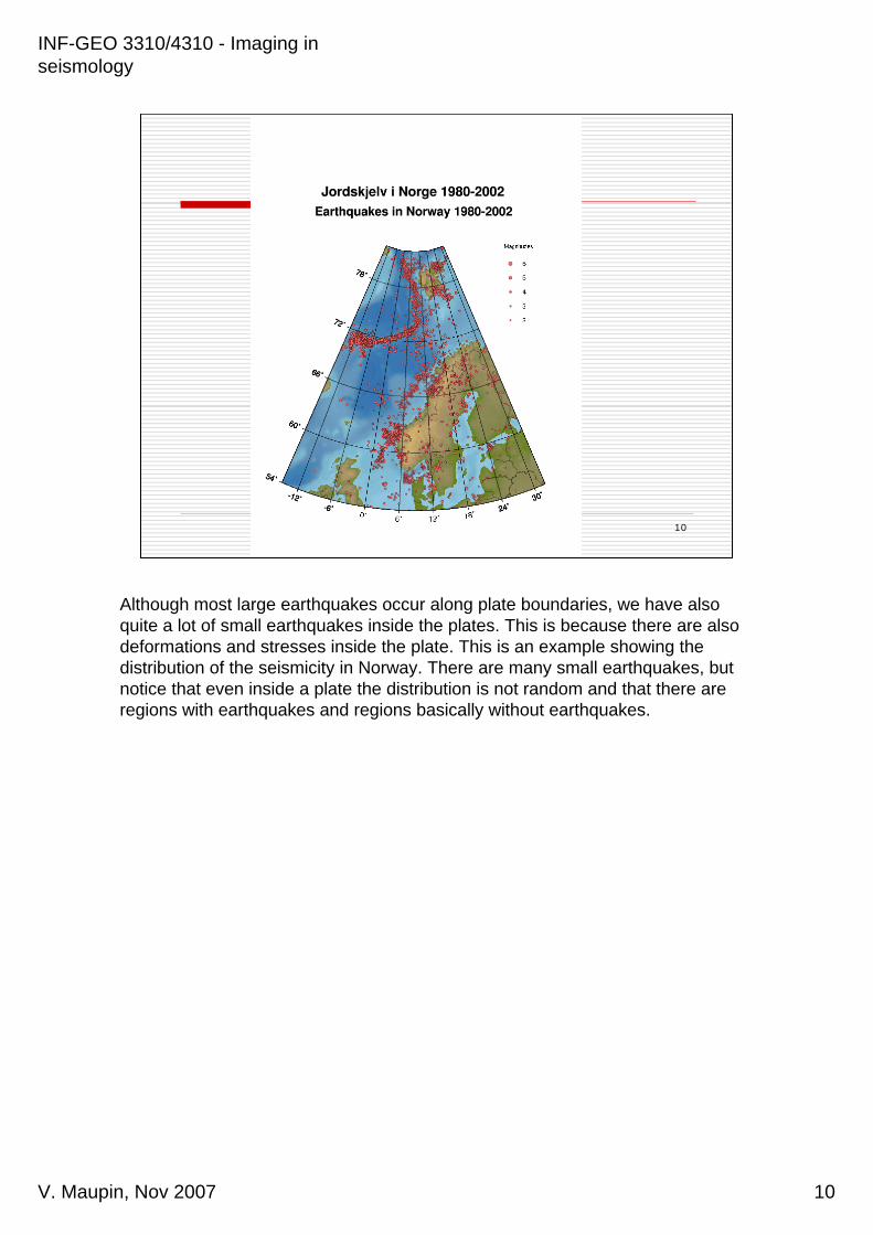
Although most large earthquakes occur along plate boundaries, we have also quite a lot of small earthquakes inside the plates. This is because there are also deformations and stresses inside the plate. This is an example showing the distribution of the seismicity in Norway. There are many small earthquakes, but notice that even inside a plate the distribution is not random and that there are regions with earthquakes and regions basically without earthquakes.

INF-GEO 3310/4310 - Imaging in seismology
V. Maupin, Nov 2007 11
11
Total number of earthquakes per year as a function ofmagnitude on theRichter-scale and amount of energy
Sumatra 2004
The amount of energy released by earthquakes is quite enormous and they are really very efficient sources of vibrations for imaging the Earth. In addition to earthquakes, it is possible to use nuclear underground explosions as source of vibration for studying the Earth. But they are of course much more seldom than earthquakes!

INF-GEO 3310/4310 - Imaging in seismology
V. Maupin, Nov 2007 12
12
As a stone which you drop in the water perturbs the surface and generates waves, do earthquakes generate seismic waves which propagate in the whole Earth.
INF-GEO 3310/4310 - Imaging in seismology
V. Maupin, Nov 2007 13
13
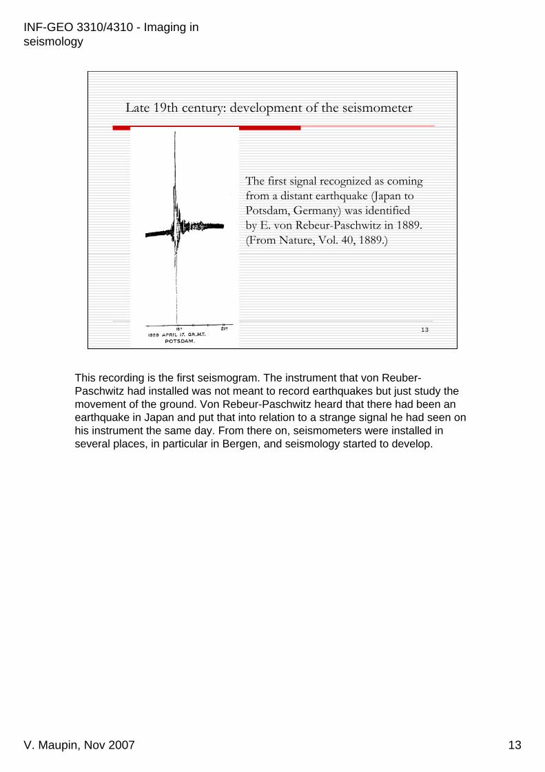
Late 19th century: development of the seismometer
The first signal recognized as coming from a distant earthquake (Japan to Potsdam, Germany) was identified by E. von Rebeur-Paschwitz in 1889. (From Nature, Vol. 40, 1889.)
This recording is the first seismogram. The instrument that von Reuber-Paschwitz had installed was not meant to record earthquakes but just study the movement of the ground. Von Rebeur-Paschwitz heard that there had been an earthquake in Japan and put that into relation to a strange signal he had seen on his instrument the same day. From there on, seismometers were installed in several places, in particular in Bergen, and seismology started to develop.
INF-GEO 3310/4310 - Imaging in seismology
V. Maupin, Nov 2007 14
14
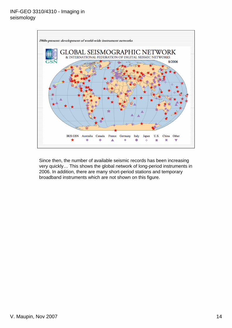
1960s-present: development of world-wide instrument networks
Since then, the number of available seismic records has been increasing very quickly… This shows the global network of long-period instruments in 2006. In addition, there are many short-period stations and temporary broadband instruments which are not shown on this figure.

INF-GEO 3310/4310 - Imaging in seismology
V. Maupin, Nov 2007 15
15
This is an example of the ground motion that one records nowadays after an earthquake at a distance of about 4000km from the earthquake. The three plots show the three components of the motion (vertical, and two horizontal directions) as a function of time. The zero time here is the time of the earthquake. The first vibrations arrive about 4 mn after the earthquake and the last ones arrive almost half-an-hour after the earthquake has occurred.
The earthquake itself lasts only a few seconds. The reason for the long duration of the seismogram is the fact that the Earth is not homogeneous and that we have many echoes. It is by studying these echoes that we can infer the structure of the Earth, or do the imaging of the Earth’s interior.

INF-GEO 3310/4310 - Imaging in seismology
V. Maupin, Nov 2007 16
16
The periods of these waves:
from around 0.01s (local earthquakes)
to 53 mn (maximum on Earth)
The period of the waves which are generated by earthquakes are large compared to the period of the other waves you have seen in this course. We usually express frequencies in mHz (milliHertz) in seismology. The wave velocities are of the order of a few km/s. This gives wavelengths varying basically from a few tens of meters to several thousand km. The resolution you can obtain from such waves is of course not very large. But you have to consider this relatively to the size of the Earth.

INF-GEO 3310/4310 - Imaging in seismology
V. Maupin, Nov 2007 17
17
What is an earthquake?Imaging: early studies and the meanstructure of the EarthP-wave tomographyNormal mode tomographySource location and time-reversal

INF-GEO 3310/4310 - Imaging in seismology
V. Maupin, Nov 2007 18
18
Wave propagation for distant earthquakes
If the Earth had been an homogenous spherical body, as on the left figure, we would have had a simple geometrical relation between the traveltimes of the P and S waves and epicentral distance (the distance along the surface of the Earth between the earthquake and the seismometer). Due to the structure inside the Earth, this relation is more complicated. The traveltime as a function of distance is actually THE major data used in imaging the Earth, both for early studies, as we will see now, and in modern P-wave tomographies as we will see in the second example.

INF-GEO 3310/4310 - Imaging in seismology
V. Maupin, Nov 2007 19
19
P
P
Ssini1/v1=sini2/v2
Refraction and conversion of waves at interfaces is a fundamental element in imaging. Here you see how a P wave incident from below at an interface is converted to an S wave. The rules for the incidence of refracted rays is called Snell’s law and is given here.

INF-GEO 3310/4310 - Imaging in seismology
V. Maupin, Nov 2007 20
20
Richard Oldham
Discovery of the Earth’s (outer) core (1906)
Much of the early studies, and many of recent studies also, are based on ray theory, which is just the geometrical optics applied to propagation in solids. The major element inside the Earth is the presence of the core. This was recognized very early, and found by observing that the arrival time of P waves with distance was not continuous, but had a jump at about 120 degrees distance. Actually the jump is rather at 100 degrees and we know today that the core is larger than what Oldham had calculated, but the principle back his discovery is still valid.

INF-GEO 3310/4310 - Imaging in seismology
V. Maupin, Nov 2007 21
21
Andrija Mohorovicic
Discovery of the MOHO discontinuity (1909)
The other discontinuity to be discovered very early was the crust-mantle boundary. This was discovered also by analyzing the arrival times as a function of distance, but much closer to the earthquake. The first wave arrival time first increases with distance with a given velocity, corresponding to the velocity in the crust (layer A here), and then increases more sharply, when the wave refracted in the mantle (layer B) starts to arrive first. This is also a simple example of how the arrival time as a function of distance can be used to image the subsurface. This technique, called refraction, is also used at smaller scale in seismics to find the depth of sedimentary layers.

INF-GEO 3310/4310 - Imaging in seismology
V. Maupin, Nov 2007 22
22
Traveltimes ofP waves at 60
to 100deg distance:
600 to 1000sec
This figure shows the observed arrival times as a function of epicentral distance for many data put together. You see that there is not only one P and one S wave, as it would have been in a simple Earth structure, but many waves, and that they are several branches in these waves. Each branch corresponds to a different type of path within the Earth. You see also that the branches are curved. The curvature tells us something about the velocity increase inside the Earth. By combining all this information, we get some information about the distribution of the waves velocity with depth with the Earth.

INF-GEO 3310/4310 - Imaging in seismology
V. Maupin, Nov 2007 23
23
Preliminary Reference Earth Model (1981)
This is the result of such an analysis, showing the velocity of the P waves, the velocity of the S waves and the density with depth. You see that we have first an increase of velocity with depth from 0 to almost 3000 km depth. This first layer is the mantle, made of silicates. Below that you have the core, where velocity is lower, still increasing with depth.

INF-GEO 3310/4310 - Imaging in seismology
V. Maupin, Nov 2007 24
24
Wave paths for P waves
Due to the increase of velocity with depth, the rays are curved into the Earth. This is a major effect which cannot be neglected when we analyze the arrival times. All the imaging studies based on geometrical optics must take into account the curvatures of the rays inside the Earth.
INF-GEO 3310/4310 - Imaging in seismology
V. Maupin, Nov 2007 25
25
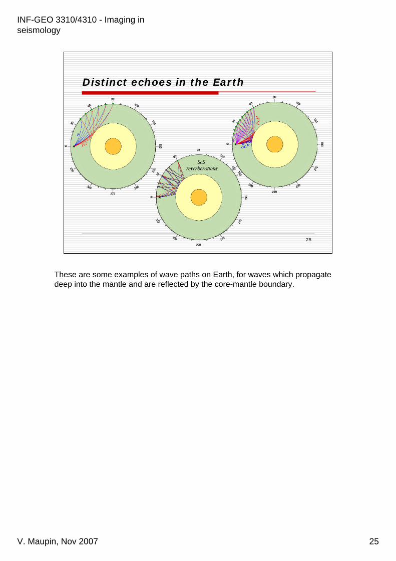
Distinct echoes in the Earth
These are some examples of wave paths on Earth, for waves which propagate deep into the mantle and are reflected by the core-mantle boundary.

INF-GEO 3310/4310 - Imaging in seismology
V. Maupin, Nov 2007 26
26
Examples of waves which propagate inside the core. Some are reflected several times inside the core. All the waves which propagate deep arrive early in the seismograms, as single arrivals, because the deeper layers have higher velocities than the upper layers. Some of the waves are quite large and observed at almost all distances from the earthquake. Some other are quite small and observed only in some special cases.
INF-GEO 3310/4310 - Imaging in seismology
V. Maupin, Nov 2007 27
27
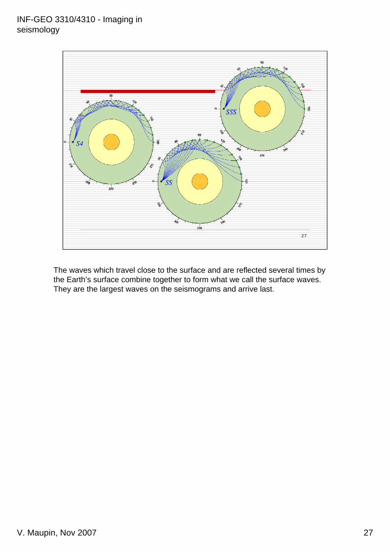
The waves which travel close to the surface and are reflected several times by the Earth’s surface combine together to form what we call the surface waves. They are the largest waves on the seismograms and arrive last.

INF-GEO 3310/4310 - Imaging in seismology
V. Maupin, Nov 2007 28
28
Surface waves: Rayleigh and Love waves
The surface waves can also been seen as waves which travel along the surface of the Earth. We have two kinds of surface waves: the Rayleigh waves which are very much like water waves or ground-roll, and Love waves which consist of a shear motion of the Earth’s surface.

INF-GEO 3310/4310 - Imaging in seismology
V. Maupin, Nov 2007 29
29
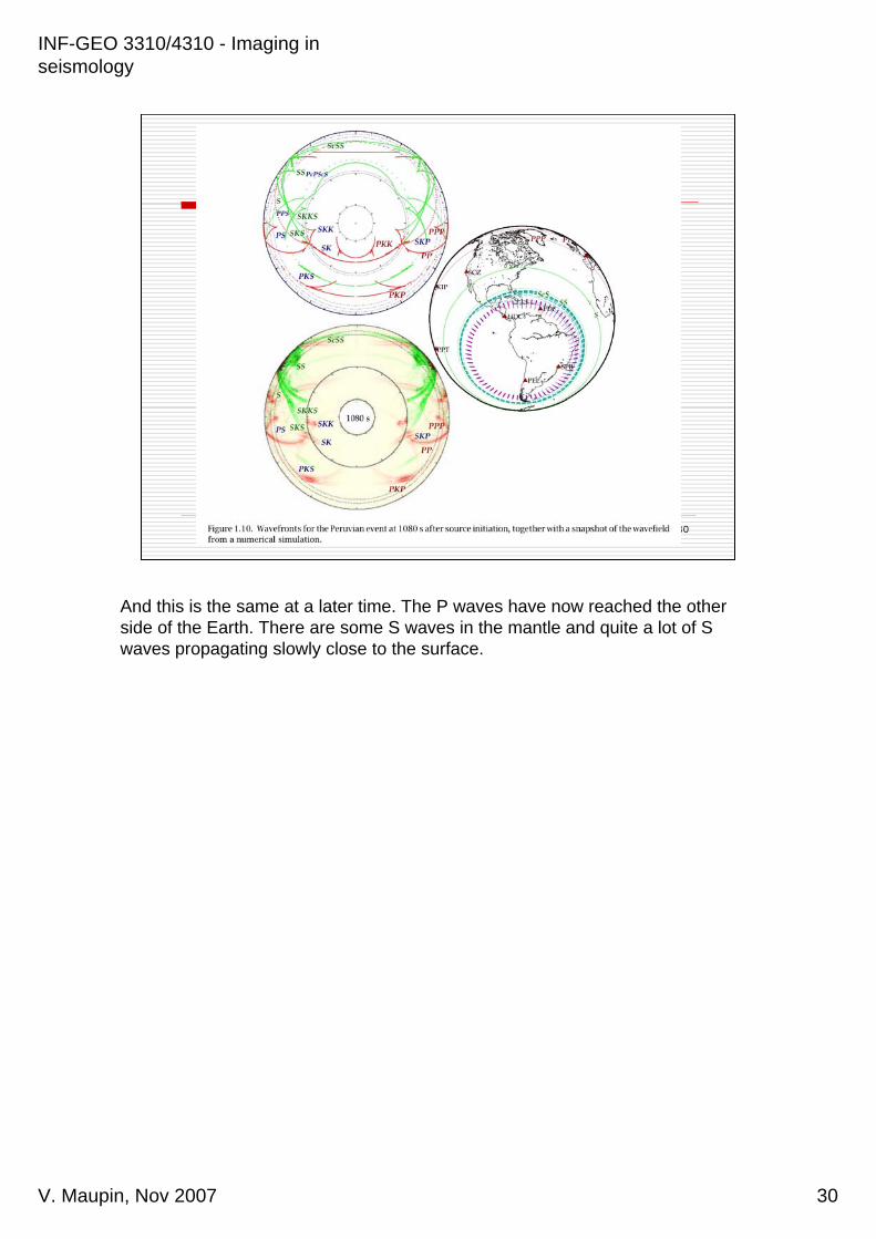
This shows all these waves propagate together both in depth and at the surface of the Earth at a given time after the earthquake. In red you have the P waves and in green the S waves.
INF-GEO 3310/4310 - Imaging in seismology
V. Maupin, Nov 2007 30
30
And this is the same at a later time. The P waves have now reached the other side of the Earth. There are some S waves in the mantle and quite a lot of S waves propagating slowly close to the surface.

INF-GEO 3310/4310 - Imaging in seismology
V. Maupin, Nov 2007 31
31
What is an earthquake?Imaging: early studies and the meanstructure of the EarthP-wave tomographyNormal mode tomographySource location and time-reversal

INF-GEO 3310/4310 - Imaging in seismology
V. Maupin, Nov 2007 32
32
On this example seismogram that we have seen before, you can see that we have many different distinct arrivals at different times. The lines show the theoretical arrival times in a simple model of the Earth without lateral variations, only depth variations. You see that they correspond quite well to the real arrivals. This is because the dominant variation of the elastic parameters in the Earth is in the depth direction. The lateral variations are much smaller than the vertical ones.

INF-GEO 3310/4310 - Imaging in seismology
V. Maupin, Nov 2007 33
33
Moonquake recording
Deep and shallow moonquake and meteoroide impactrecording on the Moon (from NASA).
The moon is much more heterogeneous than the Earth. These plots show the recordings of moonquakes and meteoroid impact at four different components of a seismometer put on the Moon by NASA. As opposed to the Earth recordings, you cannot identify different waves or echoes on these seismograms. You have basically a very complicated record which does not allow for any sensible imaging of precise structures.

INF-GEO 3310/4310 - Imaging in seismology
V. Maupin, Nov 2007 34
34
Traveltimes ofP waves at 60
to 100deg distance:
600 to 1000sec
We have seen before that the traveltimes of the waves vary with distance and that this variation gives us information about the structure of the Earth. If the Earth was perfectly spherical with no lateral variations, all the arrivals would fit perfectly with the lines calculated for the Earth model here. You see that here are some points which fall outside. This is due to lateral variations of the velocities inside the Earth. The mean structure of the Earth is very well known now, and imaging studies concentrate on imaging the lateral variations.
INF-GEO 3310/4310 - Imaging in seismology
V. Maupin, Nov 2007 35
35
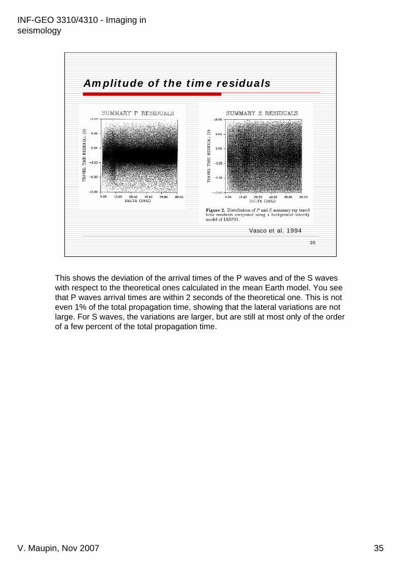
Amplitude of the time residuals
Vasco et al. 1994
This shows the deviation of the arrival times of the P waves and of the S waves with respect to the theoretical ones calculated in the mean Earth model. You see that P waves arrival times are within 2 seconds of the theoretical one. This is not even 1% of the total propagation time, showing that the lateral variations are not large. For S waves, the variations are larger, but are still at most only of the order of a few percent of the total propagation time.
INF-GEO 3310/4310 - Imaging in seismology
V. Maupin, Nov 2007 36
36
Traveltimes, origin times and locations
The arrival time at a station depends on:Velocity along the pathOrigin time of earthquakeEpicenter of earthquakeDepth of earthquake
In addition, errors due toClock problemsReading errorsLocalized strong heterogeneities in thecrust below the station

INF-GEO 3310/4310 - Imaging in seismology
V. Maupin, Nov 2007 37
37
ISC database
About 2500 stations report to the ISC (International Seismological Centre): thousands of earthquakes/year, millions of traveltimes.Primary objective: earthquakelocation and catalogueSpin-off: global arrival time database

INF-GEO 3310/4310 - Imaging in seismology
V. Maupin, Nov 2007 38
38
Principle of tomography
All the waves whichtravel through the
slow region will arrivelate.
The amount of delayon each ray dependson the strength of theheterogeneity and its
size.
Using the arrival times at the rays, we can reconstruct the distribution of the velocity inside the body.

INF-GEO 3310/4310 - Imaging in seismology
V. Maupin, Nov 2007 39
39
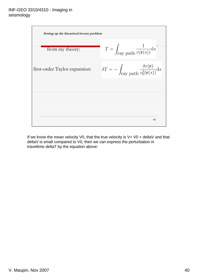
Setting up the linearized inverse problem
from ray theory:
The arrival time depends on distance divided by velocity along the whole path
INF-GEO 3310/4310 - Imaging in seismology
V. Maupin, Nov 2007 40
40
Setting up the linearized inverse problem
from ray theory:
first-order Taylor expansion:
If we know the mean velocity V0, that the true velocity is V= V0 + deltaV and that deltaV is small compared to V0, then we can express the perturbation in traveltime deltaT by the equation above:

INF-GEO 3310/4310 - Imaging in seismology
V. Maupin, Nov 2007 41
41
Setting up the linearized inverse problem
from ray theory:
first-order Taylor expansion:
“parameterization”:
The velocity variations inside the structure is what we are trying to find. We have somehow to transform this three-dimensional quantity into a few parameters which can be handled by a computer. This can be done by expressing the velocities on a basis of functions.

INF-GEO 3310/4310 - Imaging in seismology
V. Maupin, Nov 2007 42
42
Parameterization, or choice of basis functions
pixels (“local”basis functions)
One common basis of functions is to use small cells. This means that we assume that each cell has a constant velocity. The size of the cells has to be chosen such that it fits with the number of rays we have and the wavelength of the waves.

INF-GEO 3310/4310 - Imaging in seismology
V. Maupin, Nov 2007 43
43
Parameterization, or choice of basis functions
spherical harmonics (“global” basis functions)
Another possible parameterization is on functions like the spherical harmonics, which is equivalent to doing a 2D Fourier decomposition of the velocity. Although it is less intuitive than the cell decomposition, it is very well adapted in global studies.

INF-GEO 3310/4310 - Imaging in seismology
V. Maupin, Nov 2007 44
44
Setting up the linearized inverse problem
from ray theory:
first-order Taylor expansion:
“parameterization”:
Unknown coefficients are constant and don’t need to be integrated:
known
Since the functions are known, the reference velocity and the ray paths are known, everything in the red ring is known and can be calculated. It is commonly assumed that the perturbations to the velocity are small and do not perturb significantly the ray path. This is of course true only at first order and some newer tomographic studies try to remove this assumption.

INF-GEO 3310/4310 - Imaging in seismology
V. Maupin, Nov 2007 45
45
Setting up the linearized inverse problem
the same eq. Applies for many data and corresp. ray paths:
introduce matrix A:
This integral can be calculated for each traveltime j and each cell i (or function i) to build a matrix which then relates the traveltime anomalies to the velocity perturbation in the different cells.

INF-GEO 3310/4310 - Imaging in seismology
V. Maupin, Nov 2007 46
46
Setting up the linearized inverse problem
the same eq. Applies for many data and corresp. ray paths:
introduce matrix A:
And this can be written very simply in vector and matrix form.
INF-GEO 3310/4310 - Imaging in seismology
V. Maupin, Nov 2007 47
47
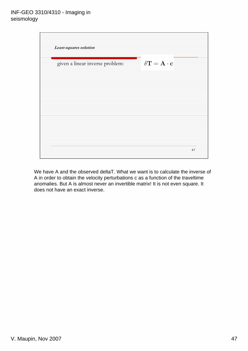
Least-squares solution
given a linear inverse problem:
We have A and the observed deltaT. What we want is to calculate the inverse of A in order to obtain the velocity perturbations c as a function of the traveltimeanomalies. But A is almost never an invertible matrix! It is not even square. It does not have an exact inverse.
INF-GEO 3310/4310 - Imaging in seismology
V. Maupin, Nov 2007 48
48
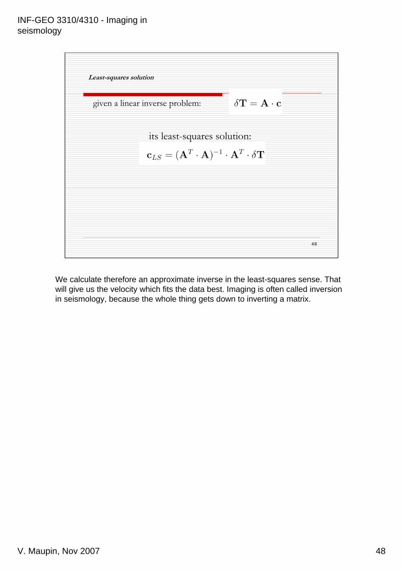
Least-squares solution
its least-squares solution:
given a linear inverse problem:
We calculate therefore an approximate inverse in the least-squares sense. That will give us the velocity which fits the data best. Imaging is often called inversion in seismology, because the whole thing gets down to inverting a matrix.
INF-GEO 3310/4310 - Imaging in seismology
V. Maupin, Nov 2007 49
49
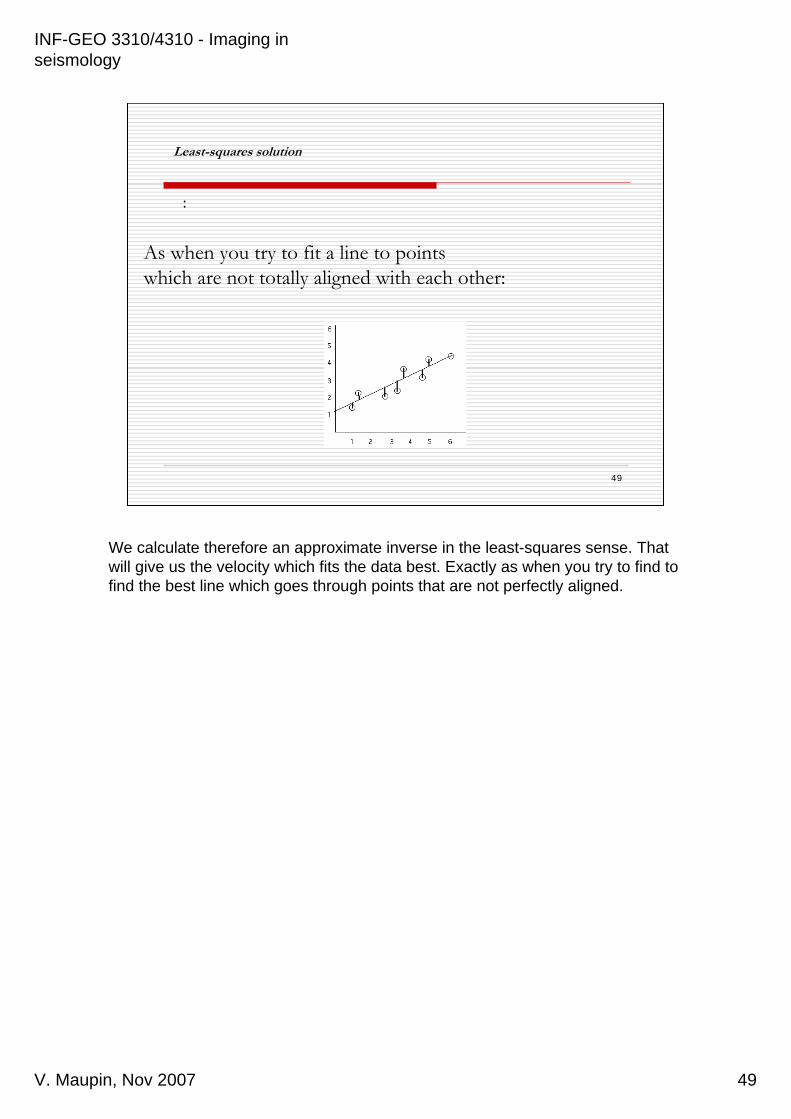
Least-squares solution
As when you try to fit a line to pointswhich are not totally aligned with each other:
:
We calculate therefore an approximate inverse in the least-squares sense. That will give us the velocity which fits the data best. Exactly as when you try to find to find the best line which goes through points that are not perfectly aligned.

INF-GEO 3310/4310 - Imaging in seismology
V. Maupin, Nov 2007 50
50
Least-squares solution
its least-squares solution:
given a linear inverse problem:
is typically solved by either:
iterative algorithms (CG, LSQR…)direct algorithms (SVD, Cholesky…)
In most cases, the A matrix is very big and you need special algorithms to perform the inversion.

INF-GEO 3310/4310 - Imaging in seismology
V. Maupin, Nov 2007 51
51
The effect of errors in the data
Small errors in thedata can be mapped
as small-scaleheterogeneities
What to keep?
Not a simple question.
One very important question is the effect of the errors on the data on the model. If you have errors on the data, they can get mapped into the structure. In the example above, we have two rays with negative errors. If we don’t know that there are errors on these data and try to explain the data by heterogeneities in the model, we have to put two small spots of low velocities (red) which are not real features of the structure. Here we have also three rays with positive errors which we have managed to explain with two spots (blue) of high velocity. In order to avoid mapping errors in the model, we need to define the amplitude of the errors we can expect on the data. This is a crucial step in the imaging process which determines indirectly the size of the features that we can get in the model.
INF-GEO 3310/4310 - Imaging in seismology
V. Maupin, Nov 2007 52
52
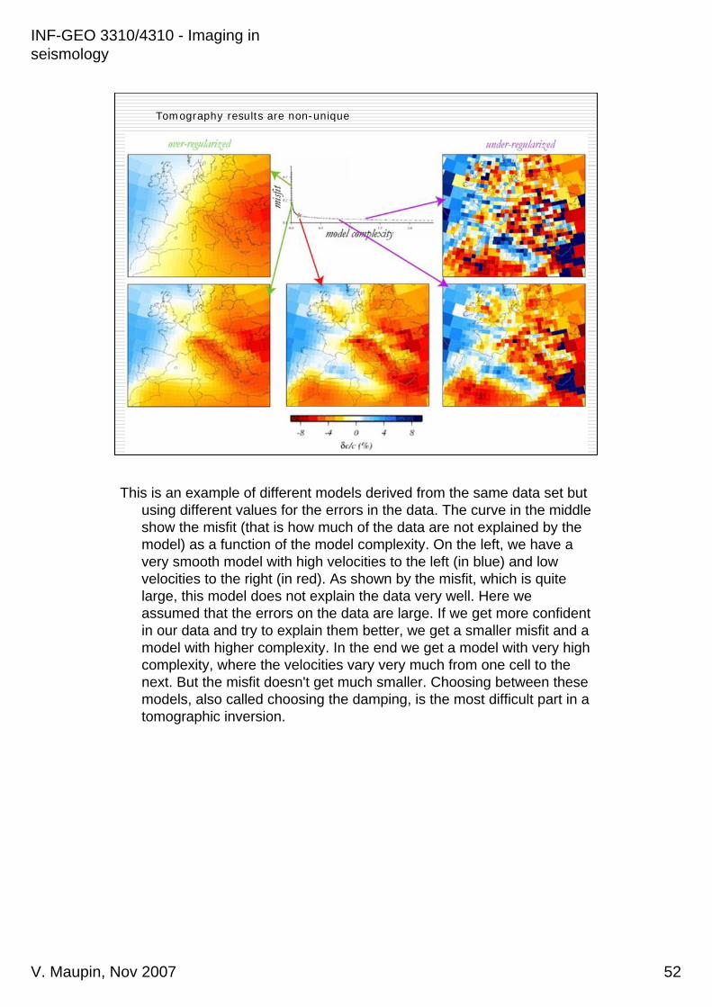
Tomography results are non-unique
This is an example of different models derived from the same data set but using different values for the errors in the data. The curve in the middle show the misfit (that is how much of the data are not explained by the model) as a function of the model complexity. On the left, we have a very smooth model with high velocities to the left (in blue) and low velocities to the right (in red). As shown by the misfit, which is quite large, this model does not explain the data very well. Here we assumed that the errors on the data are large. If we get more confident in our data and try to explain them better, we get a smaller misfit and a model with higher complexity. In the end we get a model with very high complexity, where the velocities vary very much from one cell to the next. But the misfit doesn't get much smaller. Choosing between these models, also called choosing the damping, is the most difficult part in a tomographic inversion.

INF-GEO 3310/4310 - Imaging in seismology
V. Maupin, Nov 2007 53
53
Effect of damping
Small-scale heterogeneitiesAmplitude of the large-scaleheterogeneitiesBasically the resolution is changed
Damping reduces the amplitude of the smal heterogeneities in the final model. It also affects, although less severely; the amplitude of the large scale anomalies. It is basically changing what we call the resolution. In conclusion, we see very directly and mathematically here how the resolution of the imaging is related to the size of the errors on the measurements.
INF-GEO 3310/4310 - Imaging in seismology
V. Maupin, Nov 2007 54
54
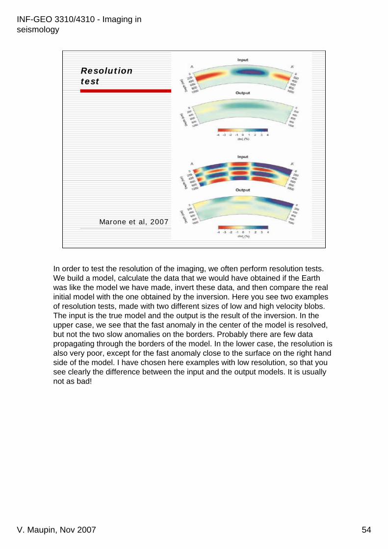
Resolutiontest
Marone et al, 2007
In order to test the resolution of the imaging, we often perform resolution tests. We build a model, calculate the data that we would have obtained if the Earth was like the model we have made, invert these data, and then compare the real initial model with the one obtained by the inversion. Here you see two examples of resolution tests, made with two different sizes of low and high velocity blobs. The input is the true model and the output is the result of the inversion. In the upper case, we see that the fast anomaly in the center of the model is resolved, but not the two slow anomalies on the borders. Probably there are few data propagating through the borders of the model. In the lower case, the resolution is also very poor, except for the fast anomaly close to the surface on the right hand side of the model. I have chosen here examples with low resolution, so that you see clearly the difference between the input and the output models. It is usually not as bad!
INF-GEO 3310/4310 - Imaging in seismology
V. Maupin, Nov 2007 55
55
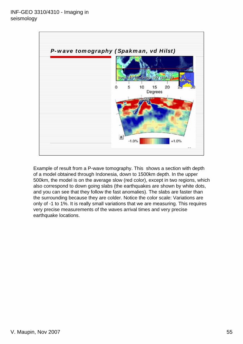
P-wave tomography (Spakman, vd Hilst)
Example of result from a P-wave tomography. This shows a section with depth of a model obtained through Indonesia, down to 1500km depth. In the upper 500km, the model is on the average slow (red color), except in two regions, which also correspond to down going slabs (the earthquakes are shown by white dots, and you can see that they follow the fast anomalies). The slabs are faster than the surrounding because they are colder. Notice the color scale: Variations are only of -1 to 1%. It is really small variations that we are measuring. This requires very precise measurements of the waves arrival times and very precise earthquake locations.

INF-GEO 3310/4310 - Imaging in seismology
V. Maupin, Nov 2007 56
56
P-wave tomography
Van der Voo et al., 1999
This is another example, through northern Asia and to a larger depth. To the right, you see the Japanese slab, with its seismicity. You see also that the fast material goes further down into the mantle than 700km (which is the maximum depth of the earthquakes). The fast material noted P is believed to come from the Japanese subduction. The fast material noted M is believed to come from an ancient subduction which occurred 200 to 150 Myears ago, at a time where East and West Asia were separated by an ocean.

INF-GEO 3310/4310 - Imaging in seismology
V. Maupin, Nov 2007 57
57
These models give us the P-wavevelocity distribution in the EarthThey are based on short-period P-waves (1Hz).

INF-GEO 3310/4310 - Imaging in seismology
V. Maupin, Nov 2007 58
58
What is an earthquake?Imaging: early studies and the meanstructure of the EarthP-wave tomographyNormal mode tomographySource location and time-reversal
Now we are going to see a rather different approach to imaging, not based on ray theory.

INF-GEO 3310/4310 - Imaging in seismology
V. Maupin, Nov 2007 59
59
We have seen before that the arrival times of waves as a function of distance between the earthquake and the station have a central position in the methods that we use to image the interior of the Earth. Now we are not going to look at the arrival time of individual waves, but look at the whole recording as a function of time and distance. The advantage of looking at the whole recording is that we keep much more information from the seismograms than when we pick just a few arrival times. In addition we use the information contained in the amplitudes of the waves, their frequency content, etc and we keep all the waves, even those with complicated wavepaths.On the figure above, you see the recording of the Sumatra earthquake of 2004 at many stations, organized as a function of increasing distance from the earthquake. At the beginning of the traces, you see (but they are very small) the P waves that we have used in the P-wave tomography just before, then S waves, then the surface waves with the largest amplitudes. All these waves have traveltimes increasing with distance. Then you have a wave noted R2 which has an arrival time decreasing with distance, a wave called R3 which arrives with a constant delay with respect to the surface waves.

INF-GEO 3310/4310 - Imaging in seismology
V. Maupin, Nov 2007 60
60
Surface waves: late, long-period and large amplitude waves
You see something similar here for another earthquake. Here the first surface wavetrain is called R1.

INF-GEO 3310/4310 - Imaging in seismology
V. Maupin, Nov 2007 61
61
R1R2
These different waves correspond to waves which propagate to the station from different sides of the Earth. R1 travels directly from the earthquake to the station. R2 travels around and arrives at the station from the other side. R3 is R1 after it has gone one time around the Earth and back to the station. One full round trip lasts about 3 hours. For very large earthquakes, the waves continue to travel around for many days.If you see that in 3D, you see that the waves are propagating away from the earthquake, converge at the antipode, propagate back to the earthquake and then diverge again etc. You see that you have a sort of pulsation of movement going back and forth on the planet. This can be seen as the eigenvibrations of the Earth.
INF-GEO 3310/4310 - Imaging in seismology
V. Maupin, Nov 2007 62
62
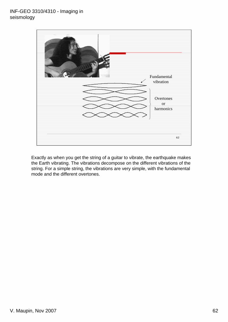
Fundamentalvibration
Overtonesor
harmonics
Exactly as when you get the string of a guitar to vibrate, the earthquake makes the Earth vibrating. The vibrations decompose on the different vibrations of the string. For a simple string, the vibrations are very simple, with the fundamental mode and the different overtones.

INF-GEO 3310/4310 - Imaging in seismology
V. Maupin, Nov 2007 63
63
Fundamentalvibration
Overtonesor
harmonics
Spectrum:
Duration of onevibration cycle or period: T
Frequency: f=1/T
If you take the spectrum of the sound made by the guitar, you will see that the spectrum has some peaks, corresponding to the different modes of the string.
INF-GEO 3310/4310 - Imaging in seismology
V. Maupin, Nov 2007 64
64
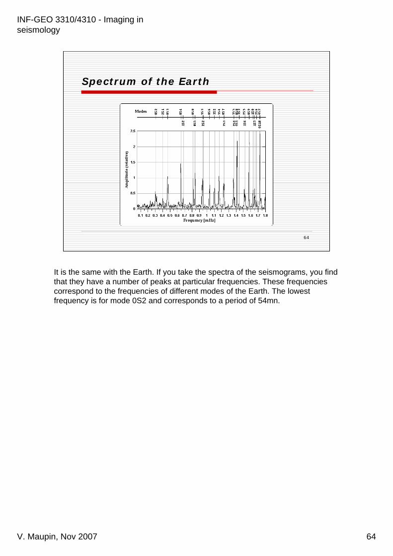
Spectrum of the Earth
It is the same with the Earth. If you take the spectra of the seismograms, you find that they have a number of peaks at particular frequencies. These frequencies correspond to the frequencies of different modes of the Earth. The lowest frequency is for mode 0S2 and corresponds to a period of 54mn.

INF-GEO 3310/4310 - Imaging in seismology
V. Maupin, Nov 2007 65
65
Normal modes
Each mode has a number and a particular way of deforming the Earth. The toroidal modes do not have any vertical component. They only produce a shear at the surface of the Earth. Three examples of toroidal modes are shown here in blue, together with their periods. Spheroidal modes have a vertical component. 0S0 corresponds to a uniform dilatation and contraction of the Earth. 0S2 to a rugby-ball type deformation.

INF-GEO 3310/4310 - Imaging in seismology
V. Maupin, Nov 2007 66
66
Sensitivity kernels of normal modes
The deformation is not only at the surface of course. Each mode has its own amplitude of deformation with depth. Mode 1S4 for example deforms the whole mantle, with a maximum at about 600km depth. Mode 6S3 has a more complex deformation involving the mantle and the core.
INF-GEO 3310/4310 - Imaging in seismology
V. Maupin, Nov 2007 67
67
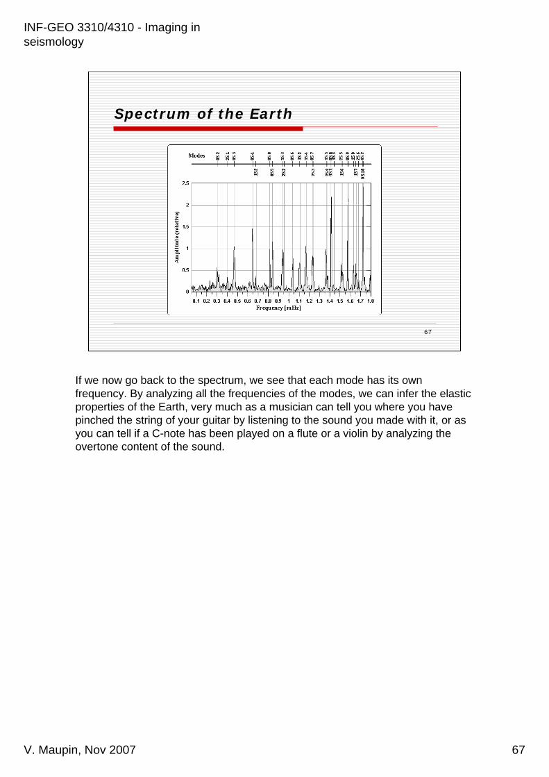
Spectrum of the Earth
If we now go back to the spectrum, we see that each mode has its own frequency. By analyzing all the frequencies of the modes, we can infer the elastic properties of the Earth, very much as a musician can tell you where you have pinched the string of your guitar by listening to the sound you made with it, or as you can tell if a C-note has been played on a flute or a violin by analyzing the overtone content of the sound.

INF-GEO 3310/4310 - Imaging in seismology
V. Maupin, Nov 2007 68
68
PREM model
Dziewonski and Anderson, 1981)
This is how our most used reference model PREM has been made. This is a better way of doing a reference model for the Earth than by analyzing many many rays because here we let the waves travel around many times, sample every single corner of the planet and average all the properties. If we take only direct P waves from earthquakes to stations, we sample some regions (with many earthquakes for example) more than others and the risk of getting a bias is larger. But we can also use the normal modes to analyze the heterogeneities of the Earth as we will see now.

INF-GEO 3310/4310 - Imaging in seismology
V. Maupin, Nov 2007 69
69
Splitting of the frequencies
If the Earth was laterally homogenous, each mode would have a single frequency. You may see here that for some modes you have two peaks or more, for example for 0S2. This is due to the lateral heterogeneity inside the Earth, which results basically in the fact that the modes do not oscillate at exactly the same frequencies at all locations.

INF-GEO 3310/4310 - Imaging in seismology
V. Maupin, Nov 2007 70
70
From Resovsky
1997
This is a map of the deviation from the central frequency for different modes. For example mode 0S3 oscillates at a slightly smaller frequency below the Pacific Ocean and Africa. This is because the wave velocity is slightly slower at these places, and it takes slightly more time for the vibration to travel at that place. The higher the order of the mode, the more detailed the maps get, because the waves get higher frequencies and have therefore a better resolution. But you see basically that they all have lower and higher frequencies in the same regions. These correspond to regions of the Earth with faster or slower material, corresponding to regions which are warmer or colder.

INF-GEO 3310/4310 - Imaging in seismology
V. Maupin, Nov 2007 71
71
From Gabi Laske
I don’t have time here to show you more in details how the imaging is done, from the spectrum of individual seismograms to the map of the frequency shifts, and then to the imaging of the structure of the Earth with depth. But I can say that this is done iteratively by taking an approximate known structure for the Earth and calculating, by least-squares, which perturbations are the best ones to explain the observed data. Many different people do this kind of imaging and we now have a good idea of the structure of the Earth, even if the different studies do no agree yet on the details. What is clear is that we have most heterogeneities in the upper 700km and in the 300kn above the core-mantle boundary. We see that the continents are usually faster than oceanic regions, that the oceanic regions get faster when they get older (because they cool). We see fast anomalies around the Pacific Ocean, related to the cold subduction slabs.

INF-GEO 3310/4310 - Imaging in seismology
V. Maupin, Nov 2007 72
72
From Gabi Laske
At the core-mantle boundary, we see the remnants of ancient subductions and we see two regions of slow material below Africa and below Central Pacific. There is no completely accepted explanation for these slow anomalies.

INF-GEO 3310/4310 - Imaging in seismology
V. Maupin, Nov 2007 73
73
Plate tectonics Mantle Convection
All this information is used to make models of how the Earth is working, what is the driving force of plate tectonics, volcanism, hotspots etc..

INF-GEO 3310/4310 - Imaging in seismology
V. Maupin, Nov 2007 74
74
What is an earthquake?Imaging: early studies and the meanstructure of the EarthP-wave tomographyNormal mode tomographySource location and time-reversal
In this last part, we are going to look at another aspect of imaging in seismology, which is the location and the study of earthquakes.
INF-GEO 3310/4310 - Imaging in seismology
V. Maupin, Nov 2007 75
75
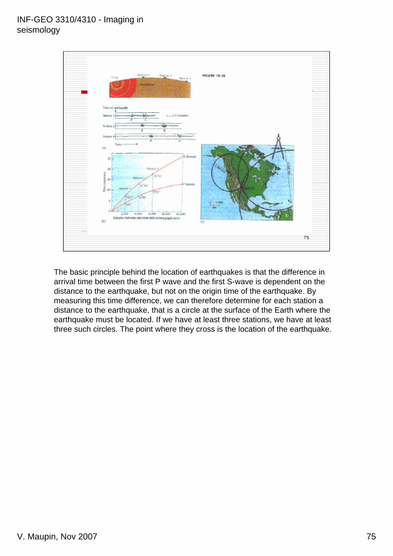
The basic principle behind the location of earthquakes is that the difference in arrival time between the first P wave and the first S-wave is dependent on the distance to the earthquake, but not on the origin time of the earthquake. By measuring this time difference, we can therefore determine for each station a distance to the earthquake, that is a circle at the surface of the Earth where the earthquake must be located. If we have at least three stations, we have at least three such circles. The point where they cross is the location of the earthquake.

INF-GEO 3310/4310 - Imaging in seismology
V. Maupin, Nov 2007 76
76
When you have the distance from each station, you can easily estimate the location of the earthquake

INF-GEO 3310/4310 - Imaging in seismology
V. Maupin, Nov 2007 77
77
We can read the arrival time of the P wave tp.If we knew the origin time of the earthquake
t0, we could write:
tp = t0 + d / Vp
which implies for the distance:
d = Vp*(tp – t0)
Mathematically, and assuming that we are not far from the earthquake and can assume a flat Earth model and a constant velocity, this can be expressed as the following:

INF-GEO 3310/4310 - Imaging in seismology
V. Maupin, Nov 2007 78
78
The arrival times of the P and S waves are:tp = t0 + d / Vp
ts = t0 + d / Vs
which implies: ts – tp = d / Vs – d / Vp= d ( 1/Vs -1/Vp )= d (Vp-Vs)/(VsVp)
This gives: d = (ts - tp) Vs Vp / (Vp – Vs)or about d = 8 (ts-tp) for d in km and t in s
and local earthquakes

INF-GEO 3310/4310 - Imaging in seismology
V. Maupin, Nov 2007 79
79
This is the simple way you can use for local events. In practice we use more than three stations, make a first guess of the location and then revisethe location and the origin time usingglobal traveltime tables until we have a location which explains the data at the best from a least-squares sense.

INF-GEO 3310/4310 - Imaging in seismology
V. Maupin, Nov 2007 80
80
Run back in time, with P waves only
Another way to look at the location of the earthquake is by back-propagation. Assume that you have simple P wave arrivals at the three stations shown here. You run back the time and you back-propagate away from the station the energy you have registered at any station. At a given time, the three circles cross each other at the epicenter location, at origin time t0 of the earthquake. This is a procedure very similar to the migration procedure that we use in seismics to find interfaces where reflections come from: by back-propagating the wavefield until it makes a sharp image.

INF-GEO 3310/4310 - Imaging in seismology
V. Maupin, Nov 2007 81
81
This is an animation showing the back-propagation of P waves from the three stations. You see that the three backpropagated waves cross each other at the location of the earthquake.

INF-GEO 3310/4310 - Imaging in seismology
V. Maupin, Nov 2007 82
82
Run back in time, with P and S waves
If you can identify the P and the S waves on the seismogram, you can also backpropagate the P waves with the P wave velocity and the S waves with the Swave velocity.

INF-GEO 3310/4310 - Imaging in seismology
V. Maupin, Nov 2007 83
83
This is the same as before but with backpropagation of the P and S waves. The S waves are in red and the P waves in blue. When you run back in time, first you get the S waves which start to backpropagate. Then the P waves. You see that all the wavefronts cross at the location of the earthquake. Errors in the velocitymodel induce errors or uncertainties in the location of the earthquakes.

INF-GEO 3310/4310 - Imaging in seismology
V. Maupin, Nov 2007 84
84
This is the same as before but I have used wrong velocities to backpropagate: I have used 5.5km/s instead of 5km/s for the P waves, and 2.5km/s instead of 3km/s for the S waves. You see that in this case the backpropagated wavefrontsdo not cross at a single point. In seismology, since both structure and source time and location are unknown, we should ideally image both at the same time. In practice, it is difficult to do it. In the best case, one can iterate: guess a location, find the structure, then refine the location, then refine the structure etc. Or one can try to use data like traveltimes for pairs of waves which are not very sensitive to the source location when imaging the structure.
INF-GEO 3310/4310 - Imaging in seismology
V. Maupin, Nov 2007 85
85
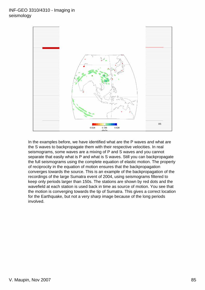
In the examples before, we have identified what are the P waves and what are the S waves to backpropagate them with their respective velocities. In real seismograms, some waves are a mixing of P and S waves and you cannot separate that easily what is P and what is S waves. Still you can backpropagatethe full seismograms using the complete equation of elastic motion. The property of reciprocity in the equation of motion ensures that the backpropagationconverges towards the source. This is an example of the backpropagation of the recordings of the large Sumatra event of 2004, using seismograms filtered to keep only periods larger than 150s. The stations are shown by red dots and the wavefield at each station is used back in time as source of motion. You see that the motion is converging towards the tip of Sumatra. This gives a correct location for the Earthquake, but not a very sharp image because of the long periods involved.
INF-GEO 3310/4310 - Imaging in seismology
V. Maupin, Nov 2007 86
86
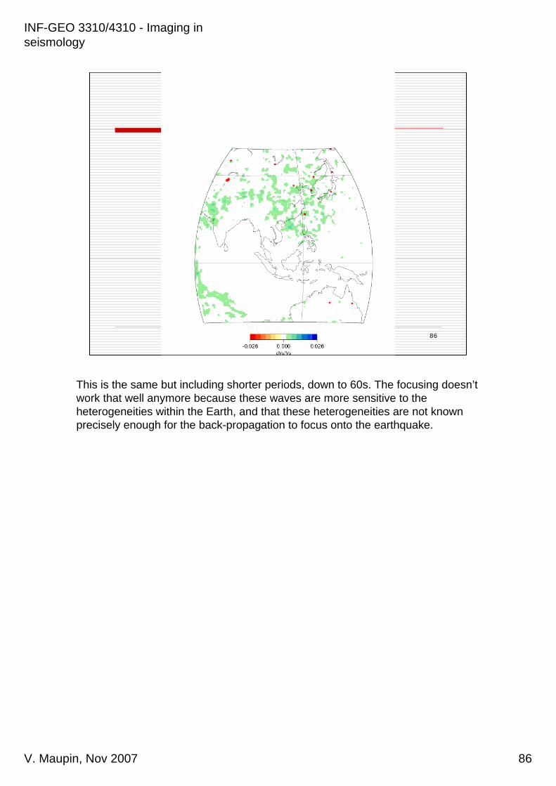
This is the same but including shorter periods, down to 60s. The focusing doesn’t work that well anymore because these waves are more sensitive to the heterogeneities within the Earth, and that these heterogeneities are not known precisely enough for the back-propagation to focus onto the earthquake.

INF-GEO 3310/4310 - Imaging in seismology
V. Maupin, Nov 2007 87
87
Conclusion
To give you an overview of imaging in seismology.Imaging of the structure and of the earthquakesRay theory is a good approximation in many casesWaveform inversion gives more informationCompared to other branches of imaging:
much is based on transmissionthe sources are natural and we have no influence on
where they are and when they occurthe number of stations is also limitedwe have developed methods to use all the information
contained in the seismograms.