www.nr.no

INF 3300, INF4300Digital Image Analysis

Thresholding

Lars Aurdal,Norsk Regnesentral,

July 24th 2006

www.nr.no

Plan

1. Automatic threshold detection:a. Ridler-Calvard’s methodb. Otsu’s method.

2. Global thresholding methods, when and why do they fail?

3. Local thresholding methods:a. Niblack’s method.b. Otsu’s method.

www.nr.no

Ridler Calvard’s method

1. This is a “classical method” originally described in the article “Picture Thresholding Using an Iterative Selection Method” by T. Ridler and S. Calvard, in IEEE Transactions on Systems, Man and Cybernetics, vol. 8, no. 8, August 1978.

www.nr.no

Ridler Calvard’s method

1. In the previous lecture we showed the following:a. If a histogram is the sum of two distributions b(z)

and f(z), b and f are the normalized background and foreground distributions respectively, z is the gray level and B and F be the prior probabilities for the background and foreground (B+F=1), then the histogram can be written p(z)=Bb(z)+Ff(z).

b. In this case the optimal threshold T will always be given by the equation:

www.nr.no

Ridler Calvard’s method

1. If you assume that b(z) and f(z) are Gaussian distributions, then this equation becomes:

2. A few algebraic manipulations will transform this into a second order equation in T:

www.nr.no

Ridler Calvard’s method

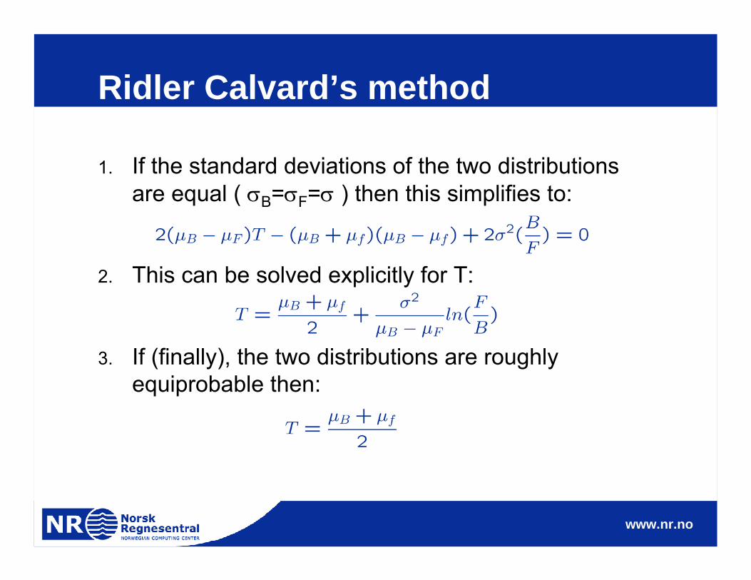
1. If the standard deviations of the two distributions are equal ( σB=σF=σ ) then this simplifies to:

2. This can be solved explicitly for T:

3. If (finally), the two distributions are roughly equiprobable then:

www.nr.no

Ridler Calvard’s method

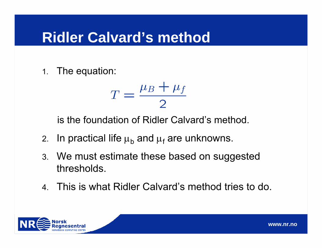
1. The equation:

is the foundation of Ridler Calvard’s method.

2. In practical life μb and μf are unknowns.

3. We must estimate these based on suggested thresholds.

4. This is what Ridler Calvard’s method tries to do.

www.nr.no

Ridler Calvard’s method

1. Assume that the histogram of the image is p(z) where z is the gray level.

2. Very simple idea:a. Start by choosing an initial threshold t0 equal to the

average gray level of the image.b. Then iterate and calculate new thresholds according to

the following formula:

c. Here μ1 is the mean value of the gray levels below tk and μ2 the mean value of the gray levels above the threshold.

www.nr.no

Ridler Calvard’s method

1. Matlab example.

www.nr.no

Otsu’s method - motivation

1. Let’s assume that you have a gray level image with L gray levels and a normalized histogram p.

2. Also assume that the image contains two populations of pixels, within each population the pixels resemble each other spectrally whereas the populations themselves differ spectrally.

3. Now find a threshold so that the pixels in the two classes that arise as a result of the thresholding are as homogeneous as possible while the two classes are as different as possible.a. Homogeneous pixels in the classes: the variance of each

class is as low as possible.b. Different classes: the difference in mean values between

the classes is as large as possible.

www.nr.no

Otsu’s method – original article

1. The following description is based on the original article by Otsu: “A threshold selection method from gray-level histograms” by N. Otsu, in IEEE Transactions on Systems, Man and Cybernetics, vol. 9, no. 1, January 1979.

www.nr.no

Otsu’s method – example imageLetter from Sir Francis Drake to Queen Elizabeth informing her of the defeat of the Spanish Armada. Our objective will be to segment out just the text. Notice that the background is not very uniform due to stains.

www.nr.no

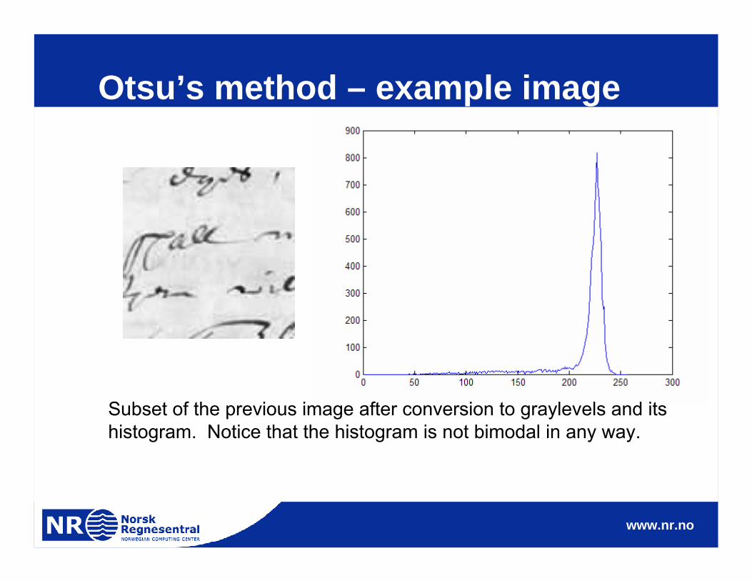
Otsu’s method – example image

Subset of the previous image after conversion to graylevels and its histogram. Notice that the histogram is not bimodal in any way.

www.nr.no

Otsu’s method

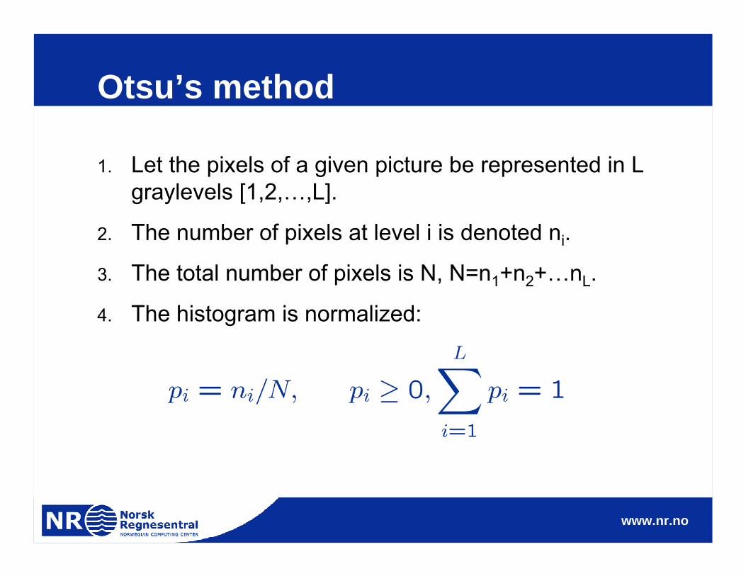
1. Let the pixels of a given picture be represented in L graylevels [1,2,…,L].

2. The number of pixels at level i is denoted ni.

3. The total number of pixels is N, N=n1+n2+…nL.

4. The histogram is normalized:

www.nr.no

Otsu’s method

1. Let’s assume that the pixels are divided into two classes, C0 and C1 (background and objects or vice versa) by a threshold at level k.

2. Thus C0 denotes pixels with levels [1,2,…,k] and C1denotes pixels with levels [k+1,…L].

www.nr.no

Otsu’s method

1. Now the probability of class occurrence is given by:

www.nr.no

Otsu’s method - example

Normalized histogram and image thresholded at k=130. At this threshold ω0=0.04 and ω1=0.96.

www.nr.no

Otsu’s method

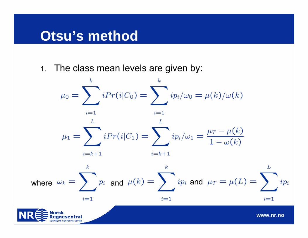
1. The class mean levels are given by:

where and and

www.nr.no

Otsu’s method - example

1. At k=130 this results in μ0=105, μ1=220 and μT=216.

www.nr.no

Otsu’s method

1. You can verify that:

www.nr.no

Otsu’s method

1. The class variances are given by:

www.nr.no

Otsu’s method - example

1. At k=130 this results in σ0=393 and σ1=301.

www.nr.no

Otsu’s method

1. Now the interesting thing is obviously to study what happens as you vary k.

www.nr.no

Otsu’s method - example

1. Consider the following measure and it’s evolution as a function of k.

2. This is a measure of the sum of the variances in the two classes

www.nr.no

Otsu’s method - example

1. Next consider the following measure and it’s evolution as a function of k.

2. This can be considered as a measure of the variance between the classes.

www.nr.no

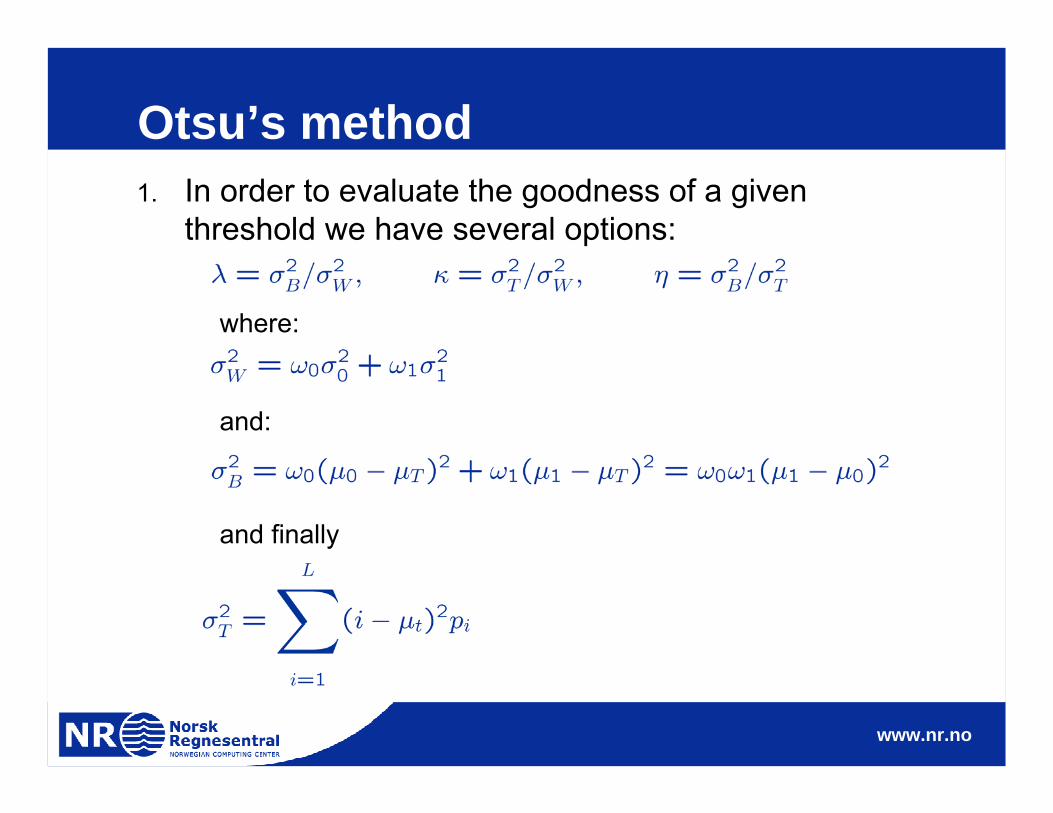
Otsu’s method1. In order to evaluate the goodness of a given

threshold we have several options:

where:

and:

and finally

www.nr.no

Otsu’s method

1. It can be verified that these criteria are related by:

since:

www.nr.no

Otsu’s method

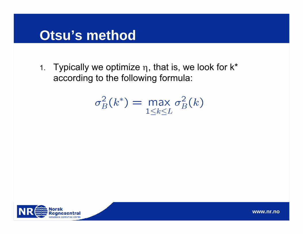
1. Typically we optimize η, that is, we look for k* according to the following formula:

www.nr.no

Otsu’s method - example

1. This shows the evolution of the measure η as a function of k.

2. It peaks for a value of179.

3. The image treholdedat this level is alsoshown.

www.nr.no

Otsu’s method - exampleFor the total image the best threshold determined by Otsu is 190. The original image and the thresholdedversion is shown to the right. Notice that the global threshold does not produce very satisfactory results.

www.nr.no

Otsu’s method

1. Matlab example.

www.nr.no

Global methods, when and why do they fail?

1. The problem observed in the last slide is very common.

2. If the image background is uneven, then finding a global threshold that provides satisfactory results can be impossible.

3. It may, quite simply, be impossible to find one single thresholdthat will separate the classes.

4. In such cases locally adaptable methods are preferred.

5. They can either treat the image in a blockwise manner or in a “sliding” window manner.

6. We will look at several such methods.

www.nr.no

Niblack’s method

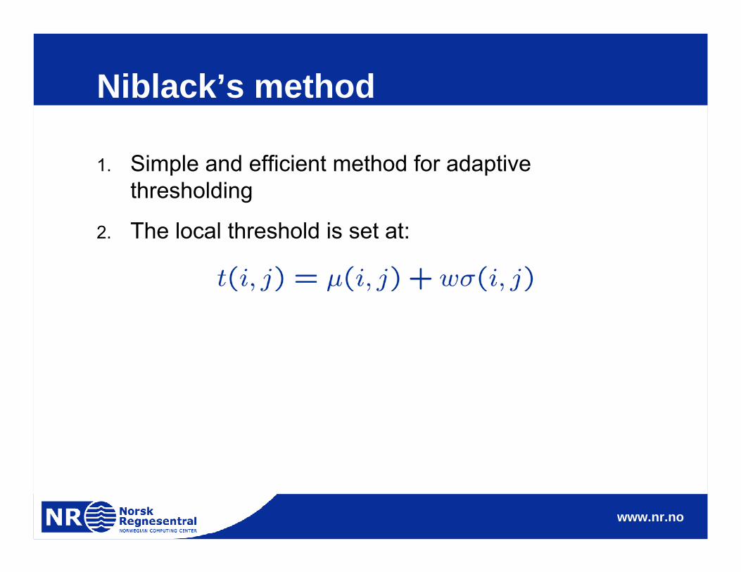
1. Simple and efficient method for adaptive thresholding

2. The local threshold is set at:

www.nr.no

Niblack’s method

1. The values for local mean and standard deviation is calculated over a local MxN window.

2. The parameters are the weight w and the window size.

3. Programming this is next weeks exercise!

www.nr.no

Niblack’s method - exampleNiblack’s method, window size 31, threshold set at 0.8 times the local standard deviation below the local mean (remember we are looking for something that is darker than it’s surroundings. Notice the improvement compared to the result when using a global threshold.

www.nr.no

Otsu’s method

1. Basically, any method for estimating the threshold can also be applied locally in a blockwise or sliding window fashion.

2. Otsu’s method is easily adaptable to this operation mode.

3. Depending on window size (and obviously the image size), a local application of Otsu can be quite computationally intensive.