inequality in public school spending across space and time

Inequality in Public School Spending Across Space and Time

This paper takes a novel time series perspective on K-12 school spending. About half of school spending is financed by state government aid to local districts. Because state aid is generally income conditioned, with low-income districts receiving more aid, state aid acts as a mechanism for risk sharing between school districts. We show that temporal inequality, due to state and local business cycles, is prevalent across the income distribution. We estimate a model of local revenue and state aid, and its allocation across districts, and use the parameters to simulate impulse response functions. We find that state aid provides risk sharing for local shocks, although slow speed of adjustment results in temporal inequality. There is little risk sharing for statewide income shocks, and the risk from such shocks to school spending is more severe in low income districts because of their greater reliance on state aid.

Suggested citation: Biolsi, Christopher, Steven G. Craig, Amrita Dhar, and Bent Sorensen. (2021). Inequality in Public School Spending Across Space and Time. (EdWorkingPaper: 21-388). Retrieved from Annenberg Institute at Brown University: https://doi.org/10.26300/6fsz-pp28

VERSION: April 2021

EdWorkingPaper No. 21-388

Christopher BiolsiWestern Kentucky University

Steven G. CraigUniversity of Houston

Amrita DharUniversity of Mary Washington

Bent E. SorensenUniversity of Houston

Inequality in Public School Spending across Space andTime

Christopher Biolsi†

Steven G. Craig‡

Amrita Dhar§

Bent E. Sørensen¶

March 31, 2021

Abstract

This paper takes a novel time series perspective on K-12 school spending. Abouthalf of school spending is financed by state government aid to local districts. Becausestate aid is generally income conditioned, with low-income districts receiving moreaid, state aid acts as a mechanism for risk sharing between school districts. We showthat temporal inequality, due to state and local business cycles, is prevalent across theincome distribution. We estimate a model of local revenue and state aid, and its allo-cation across districts, and use the parameters to simulate impulse response functions.We find that state aid provides risk sharing for local shocks, although slow speed ofadjustment results in temporal inequality. There is little risk sharing for statewideincome shocks, and the risk from such shocks to school spending is more severe in lowincome districts because of their greater reliance on state aid.

JEL: I22, H72, H77

∗This paper has benefitted from excellent comments from the Editor and two excellent referees. We alsobenefitted from comments at the meetings of the Allied Social Science Association, the European EconomicAssociation, the Oxford Education Research Symposium, the Public Choice Society, the Regional ScienceAssociation, Texas Camp Econometrics, the Econometric Society (North American Meetings), the Institutefor Public Policy and Economic Analysis Network (IPPEAN), the Kentucky Economic Association, theMidwest Macro group, the Urban Economics Association, and the Western Regional Science Association.Seminar participants at the University of Houston provided useful feedback.†Western Kentucky University; [email protected]‡University of Houston; [email protected]§University of Mary Washington; [email protected]¶University of Houston and CEPR; [email protected]

1 Introduction

Over the last forty years, U.S. state governments have attempted to reduce spending dis-parities between school districts in K-12 education financing. While the initial impetus forthese attempts arose from the courts, starting with the Serrano v. Priest decision in Cal-ifornia in 1976, most states—even those that have avoided court decisions—now use someform of income-conditioned grants. A substantial economic literature has studied inequalityin school spending, but it has been less appreciated that school spending varies over time.Our goal is to empirically model the variation in school spending over time and its impacton inequality between cohorts of students. Being income-conditioned, state aid partly offsetsthe impact of purely local income shocks on local school taxes (“local revenue”) and servesas a mechanism for risk sharing across school districts, especially at longer horizons. Stateaid, however, is positively correlated with state-level income shocks which affect all districts,leaving school spending vulnerable to such shocks.

To characterize the dynamics of school system finances, we use data from 8,676 inde-pendent school districts in the United States from 1992 to 2014, focusing on intertemporalfluctuations in school spending caused by income fluctuations. The dynamic patterns inschool spending and their dependence on state-level and local income shocks have not beenstudied in detail before. Local income shocks are found to be as likely to be negative (or pos-itive) in relatively wealthy school districts as in relatively poor school districts, so a studyof risk sharing between districts is quite separate from a study of redistribution betweenrich and poor districts. As districts change their position in the income distribution, theallocation of aid will change and have dynamic implications.

School spending is mainly financed by local revenue and state aid, and we constructa model of state and local government behavior with an objective function for each levelof government.1 For the state, we model the choice between school spending and lowertaxes while allowing for habit formation, and we model preferences for equality in spendingacross school districts. For the local school district, we model the choice between schoolspending and lower taxes while allowing for habit formation, and we model the preferencesfor offsetting state aid. We do not attempt to identify “natural experiments” and we do notmodel the many constraints that school districts operate under, so we do not consider thisa structural model of state and local agents. We interpret the results as showing reactionsto exogenous income shocks and, in particular at the local level, the estimates may bebiased due to migration of wealthier families to school districts with increases in schoolspending. The model is designed to capture salient patterns in school spending over thebusiness cycle and interprets the patterns in terms of declining marginal utility of state aidand local school revenue as well as habit persistence, which captures the gradual adjustmentof spending found in the data. Decisions are made by politicians, courts, voters who replacestate representatives and school boards, etc., rather than by a single agent, but we still findit meaningful to study if this decision process prioritizes school spending more when it islow (captured as concave utility of “the government”), and if it leads to slow adjustment

1Federal aid is comparatively small, and we ignore it in the present analysis. The federal governmentindirectly smooths school spending as federal taxes and transfers smooth state-level income shocks to grossstate product as documented by Asdrubali, Sørensen, and Yosha (1996), but in this paper we take stateincome as exogenous to school aid.

1

(“habit formation”), and if poorer districts gets more funds (“utility from equalization”).As politicians and judges and school boards serve for limited amounts of time, we find itunattractive to couch decisions in term of intertemporal preferences and we assume myopicdecision making.

The first-order conditions from the model deliver three equations that we take to thedata, obtaining highly statistically significant parameter estimates. We display results frompooled regressions and our findings are thus showing average patterns for the U.S. states,although we also show results for pre- and post-schooling reforms. We simulate the modelusing the empirical parameter estimates and assuming exogenous income shocks. The steadystate distributions are similar to the empirical distributions which indicates that estimationbias is not severe.2

Using simulated data, we provide a detailed picture of how local revenue and state aidinteract dynamically following income shocks. First, we simulate impulse response functions,which show how state aid and local revenue react to local and statewide income shocks whileaccounting for how state aid and local revenue depend on each other. Second, we highlightthat there is significant variation in school spending between cohorts within the same schooldistrict. Third, we find the incidence of district-level income shocks on after-tax local income,school spending, and state aid (which, via taxes, are transfers from other districts) in theshort and long run. Fourth, we analyze recent changes in school finance systems and findthat efforts to equalize school spending may exacerbate intertemporal disparities.

In order to provide intuition for our results, we present two examples which illustratewhat we try to capture with our model. Youngstown, Ohio, had substantially lower incomegrowth over 1995–1998 than Ohio as a whole (7.1 percent versus 11.0 percent). As a result,local revenue declined by 5.0 percent (of initial school spending in 1995), which was morethan compensated for by state aid increasing by 8.6 percent. State aid is ultimately financedby taxes on all districts in Ohio, so other school districts in the state shared the idiosyncraticincome shock to Youngstown. In the case of statewide shocks, school districts cannot sharethe aggregate risk. Consider the South San Antonio Independent School District in BexarCounty, Texas. State income per capita fell by 1.1 percent in 2013, though it barely changedin Bexar County and, as a result, state aid per student fell by close to 1.6 percent of 2012school spending. Local revenue increased by 0.3 percent (of initial school spending) to partlyoffset this loss of aid, but it was not sufficient to prevent a substantial drop in school spendingeven if local income changed little.

Dupor and Mehkari (2015) develop a model in which school districts behave as optimiz-ing consumers. They focus on school districts and treat revenue as exogenous, while wemodel school spending and the interactions between school districts and state governmentsas endogenous. Our paper also relates to the work of Fernandez and Rogerson (1996) andFernandez and Rogerson (1998) in that it examines the distribution of school spending acrossthe income distribution. These authors consider the long-run dynamic effects of schoolingon migration and the future income of students—issues we do not touch upon.

The paper proceeds as follows. Section 2 describes our data. Section 3 develops themodel and the resulting estimating equations for total state aid, for its distribution across

2We also show results from Granger causality tests, which indicates that reverse causality exists but isminor.

2

districts, and for local revenue. Section 4 reports our empirical estimates, while Section 5shows the steady-state allocations, impulse response functions, and dynamic incidence ofincome shocks. Section 6 performs the analysis splitting the sample into the periods beforeand after school finance reforms. Section 7 concludes.

2 Data

Education in the United States is the responsibility of state governments, which decide onthe organization of local education. 45 states partially or completely devolve responsibilityto single purpose independent school districts. These school districts, with separately electedboards, act within constraints imposed by state governments, but in general choose the levelof property tax rates, debt, and the distribution of funds to individual schools. For virtuallyall school districts in the United States, the local tax base is the value of property, whichit could be argued created the environment resulting in education resource disparities. Theother school district organizational form, with the exception of the statewide school districtin Hawaii, is one where education is undertaken as part of the responsibility of generalpurpose local government, typically a city (Fischel, 2009). For simplicity, and consistentwith their dominance in the United States, we use only the independent school districts forour analysis.3 We collect data on revenue by source, enrollment, and current expenditurefor independent school districts for the years 1992 to 2014, using the U.S. Census Bureau’sAnnual Survey of School System Finances.

We delete districts with less than 100 students and a small number of school districtsfor which the county indicator in the Census data changes at some point over the sample,which is possible if a school district spills over county lines. To obtain a balanced panel, weexclude districts that are not present in the data for the entire sample. Because the CensusBureau’s School System Finance data provides less coverage for the fiscal years 1993 and1994, this entails removing a number of district-year observations that would otherwise meetour criteria.4

These exclusions leave us with a panel of 8,676 independent school districts observed atthe annual frequency over 23 years in 45 states, resulting in 199,548 district-year observations—see Appendix Section A for details by state.5 On average, our sample includes 67 percent ofthe district-year observations available in the raw data, ranging from 64.5 percent of thoseappearing in the 1992 file to 77.4 percent of those in the 1994 file. Our final sample alsocontains 72.9 percent of total enrollment across all districts and years, and the share ofenrollment by year ranges from 72.4 percent in 2000 to 76.7 percent in 1994.

Independent school districts come in four types by purpose. Most are unified, meaning

3We use the indicator for independence that is encoded in the district identification variable for eachschool district by the Census Bureau. Our focus on states that at least partially use independent schooldistricts implies that we exclude all school districts from Alaska, Hawaii, Maryland, Virginia, North Carolina,and the District of Columbia.

4There are a small number of school districts where local revenue or state aid had a value of zero in atleast one year. We assign these observations a nominal $1000, but the results are robust to dropping themas shown in Appendix Table ??.

5There is a wide variety in the number of school districts across states, with 3 in Rhode Island and over900 in Texas.

3

that they comprise both elementary and secondary schools, while others may be elementaryor secondary only. 86.6 percent of the district-year observations are unified, while 10.0percent are elementary-only, and 3.1 percent are secondary-only. The final 0.3 percent arevocational school districts.

We model both state and local education expenditure as depending on income. Usingincome has the advantage that it is being uniformly measured across the country and itis measured at both state and school district levels. Collected property taxes are endoge-nous as school districts choose the tax rate, while measurement of the property tax baseis inconsistent across school districts because it varies significantly with how appraisals areconducted, and this issue is particularly problematic for commercial property. State govern-ments usually do not use property taxes but rely on sales and income taxes.6 The simulationof the model is much simplified by letting both local school revenue and state aid depend onincome, rather than, say, modeling property taxes and adding separate shocks (correlatedwith income) to the property tax base in order to generate local revenue fluctuations. Forcompleteness, we include regressions of local school spending on growth in house prices;see Appendix Table D2. For those regressions, we use standardized coefficients where theregressors are normalized by their standard deviation and we report our main specificationusing county-level income with standardized coefficients as well. The coefficients can thenbe compared across the two specifications in terms of their impact on the fluctuations inthe dependents variables. The estimated coefficients found using house prices are similar tothose found using income, so the general patterns found regarding school spending over thebusiness cycle seem robust.

Table 1 provides statistics on personal income at the school district and state levels.We assign each school district the per capita personal income of the county in which it ispredominantly located, which we refer to as “district income.” County-level personal incomefrom the Bureau of Economic Analysis is available for the entire time period of our analysis.The Census Bureau’s American Community Survey (ACS) makes income available by schooldistrict, but these data are only available from 2009 and on, implying that the sample iswithout any recessions. For completeness, we report a full set of results using district income,rather than country income, in Appendix G. The results are quite similar, except that withthis income variable local revenue is somewhat less sensitive to local income.

Table 1 also gives summary statistics for the other key variables in our analysis. Ourmeasure of “school spending” is what the Census terms “Current Expenditure” (i.e., wedo not include capital spending). Table 1 shows that school spending is roughly equal tothe sum of state aid and local revenue. In the model that we develop in Section 3, wewill explicitly define school spending as the sum of these two variables. School spending isfinanced roughly half by local taxes and half by state aid, and we ignore federal aid becauseit is a small fraction of total school revenue and it is almost exclusively directed towardsspecialized functions such as school breakfast and lunch.7 On average, state governmentsprovide 47.6 percent of total revenue as aid, local governments provide 45.6 percent of total

6Hoxby (1998) shows that per capita income predicts school spending even after controlling for propertyvaluations in a linear regression and that income in some decades is the more significant predictor.

7The primary concern with the omission of federal aid is Title I aid for low-income districts. Title I aid issmall enough that our results are not sensitive to its inclusion and school food aid is not generally fungiblewith other school expenditures.

4

revenue, and the rest is provided by the federal government. Capital outlays are about10 percent of total revenue. Table 1 also demonstrates the significance of balanced budgetconstraints as school districts typically spend all of their revenue. The average (acrossdistricts) standard deviation across time is substantial at a magnitude of about half of theaverage (over time) standard deviation across districts for most variables, including schoolspending. The bottom panels of Table 1 report growth rates, and it is apparent that district-level income is much more variable than state-level income as one would expect from theLaw of Large Numbers if idiosyncratic district income shocks are not highly correlated.

Figure 1 shows the (average) relation between our central variables and district levelincome. The figure plots time-averaged real outcomes per student as a function of time-averaged district income per capita using all of the independent school districts in our sam-ple across the 45 states after subtracting state-specific averages and adding back the overallaverage.8 Panel (a) shows an almost linear relation between local income and local rev-enue, while Panel (b) shows a declining convex relation between local income and state aid.Panel (c) shows the resulting level of school spending by income and reveals for an averagestate a convex shape with wide differences in spending across school districts; however, mostdifferences are to be found for middle- or high-income districts. For low-income districts,school spending increases only weakly, if at all, with income due primarily to state aid beingaimed at low-income districts.

Table 2 reports the sources of fluctuations in total school revenue and it is apparent thatvariation in state aid is as important as variation in local revenue for the dynamics of schoolspending.9 As we will show, state aid may fluctuate to offset idiosyncratic local incomeshocks or because of state-level income shocks.

State aid to a district changes partly because the income distribution across districtschanges. Table 3 shows the transition matrix for quintiles using the five-year moving averageof per capita district income from 1992 to 2014, and it is clear that districts can experiencesubstantial changes in their position in the income distribution within the state. Mobility ofdistricts between quintiles is largest for the middle three; for example, of the districts in themiddle-income quintile at the beginning of our sample, only 35 percent are still in the middlequintile by the end of our sample. But even for districts in the top or bottom quintiles, thereis significant mobility.

We evaluate the level of school spending by cohort assuming students do not changeschool districts. That is, we sum the spending of the school district over 13 years of K-12education and assume a student is exposed to the average level of spending each year. Weperform this calculation for all complete cohorts, consisting of students that begin schoolin the years between 1992 and 2002 and summarize the results in Table 4, which reports

8Because the number of school districts is very large, we compress the information and use binned scattergraphs, where we plot the outcomes against income which is sorted and collected into 100 quantiles on thex-axis. The corresponding value on the y-axis is averaged over the observations with income in that quantile.

9Because Total Revenue= State Aid+Local Revenue+Federal Aid, the variance of total revenue is thesum of the covariances of total revenue with state aid, local revenue, and federal aid, which implies thatOLS coefficients of regressions of each of these three components on total revenue sum to unity. The OLScoefficients have the interpretation of the fraction of variance explained (in a non-causal sense) by therelevant variable and provide measures of relative importance in explaining fluctuations in total revenue.See Asdrubali, Sørensen, and Yosha (1996) for further details.

5

Table 1: Summary Statistics for Key Variables: Total Sample

Variable Mean Std Dev 1 Std Dev 2(across districts within years) (across years within districts)

Per-Student Values (000s of 2009 dollars)

Total Revenue 10.74 3.80 2.08State Aid (District-Level) 5.11 2.38 1.24Local Revenue 4.90 3.86 1.17School Spending (District-Level) 9.02 2.78 1.56Revenue from Federal Govt 0.74 0.85 0.35Capital Outlay 1.05 1.89 1.44

Per-Capita Values (000s of 2009 dollars)

County Personal Income 30.55 7.33 7.88District Personal Income 61.41 21.40 2.51State Personal Income 35.60 5.49 4.38

Percentage Point Growth in Per-Student Values

Total Revenue 2.13 8.71 9.93State Aid 2.88 15.89 21.01Local Revenue 1.49 14.73 18.62School Spending 2.02 6.06 6.94

Percentage Point Growth in Per-Capita Values

County Personal Income 1.85 4.93 5.11District Personal Income -0.13 4.65 3.86State Personal Income 1.74 1.60 2.44

As Share of Income

Total School Spending 4.3% 1.9% 1.6%Total State Aid 1.8% 0.9% 0.2%

Notes: The table reports summary statistics of the different types of revenue and income for the sample of

8,676 independent school districts in the United States for the period 1992 to 2014 (199,548 district-year

observations). Values for levels are expressed in thousands of 2009 dollars per student (for the education

variables) or 2009 dollars per capita (for the income variables). “Std Dev 1” is defined as the average across

years of [(1/D)∑d(Xd,t−Xt)

2]1/2. “Std Dev 2” is defined as the cross sectional average of [(1/T )∑t(Xd,t−

Xd)2]1/2. For education variables, the denominator for each variable is the number of students in district

d in year t. For income variables, the denominator for each variable is the total population in county c or

state s in year t or total households in district d. The correlation coefficient between log real county income

per capita and log real district income per household net of state and year effects is 0.78.

6

Figure 1: Average School Spending, Local Revenue, and State Aid by Income

34

56

78

Loca

l Rev

enue

per

Stu

dent

20 30 40 50Real District Personal Income per Capita (000s)

(a) Local Revenue per Student

34

56

7St

ate

Aid

per S

tude

nt


(b) State Aid per Student

910

1112

13To

tal S

choo

l Spe

ndin

g pe

r Stu

dent


(c) School Spending per Student

Notes: The figure plots the average of each district’s local revenue, state aid, and school spending (all in

per student terms) over the sample period (1992–2014) against the average of its per capita income over

the sample period, along with a fitted quadratic regression line controlling for average state effects. The

figures are binned plots where income is sorted and averaged into 100 quantiles and the data on the y-axes

are averaged over the observations with income in the relevant bin. The figure excludes 413 districts where

income per person averaged more than $51.5 thousand or less than $19.2 thousand, as well as those districts

(51) spending $20 thousand more than the state average.

7

Table 2: Variance Decomposition of Total Revenue of School Districts (Percent)

Revenue Source (1) (2) (3)

State Aid 42.5 42.4 42.8(3.7) (3.7) (3.8)

Local Revenue 43.4 43.7 42.9(2.6) (2.6) (2.6)

Federal Aid 14.1 13.9 14.3(4.8) (4.9) (4.8)

Year Fixed Effects No Yes NoDistrict Fixed Effects No No Yes

Notes: The table reports coefficients estimated from regressions of ∆Yd,t = α+ β∆Total Revenued,t + εd,t,

where Yd,t denotes, sequentially, real state aid per student in district d in year t, real local revenue per

student in district d in year t, and real federal revenue per student in district d in year t. Each coefficient

represents the share of overall variation in total revenue of district d in year t accounted for by each source

of total revenue. Standard errors are clustered at the district level and are reported in parentheses.

Table 3: Transition of School-District Income Between State-Specific Income Quintiles

2010–20141992-1996 Q1 Q2 Q3 Q4 Q5Q1 0.77 0.18 0.02 0.02 0.01Q2 0.09 0.52 0.30 0.07 0.02Q3 0.07 0.23 0.35 0.27 0.08Q4 0.03 0.09 0.21 0.48 0.20Q5 0.01 0.03 0.07 0.17 0.71

Notes: Each cell of the table reports the percentage of school districts in the state income quintile given

by the row header averaged over 1992 to 1996 that is in the state income quintile indicated by the column

header averaged over 2010 to 2014.

8

that the average spending per student is about $118 thousand in real 2009 dollars. Thecohort calculation allows for smoothing over the 13 years if lean years are compensated byabundant years but despite that, the within-district cohort standard deviation is more than28 percent of the annual average cross-sectional standard deviation. In more than threepercent of the cohorts, students are subject to lower spending than their peers starting theprior year. Further, despite the fact that the average growth in per-student spending of 2.02percent is greater than average income growth, in over a quarter of the cohorts, students areeducated in school districts where school spending grew more slowly than income.

Table 4: Summary Statistics of School Spending per K-12 Cohort

Total District-Cohort Observations 95,436Average Spending by School Districts over Primary/Secondary School Career $118,199.40Average Across-District Standard Deviation $33,553.15Average Within-District Standard Deviation $9,510.82District-Cohort Observations Exposed to Less Spending than Previous Cohort 3,188 (3.7% of total)District-Cohort Observations Exposed to Less Spending than Cohort 5 Years Prior 556 (1.1% of total)District-Cohort Observations in which Spending Grows more Slowly than Income over 1 Year 27,403 (31.6% of total)District-Cohort Observations in which Spending Grows more Slowly than Income over 5 Years 13,464 (25.9% of total)

Notes: The table reports summary statistics for school spending (measured in 2009 dollars per student) that

students would be exposed to over the course of their entire K-12 education career. The table includes only

complete cohorts, covering students entering kindergarten between 1992 and 2002. The calculations assume

that a student stays in the same school district for 13 years. The last four rows of the table show the number

of district-cohort observations who, relative to older cohorts (one year and five years older), received lower

spending or had spending growth slower than income growth. The percentages in parentheses are calculated

using the appropriate comparison cohorts.

2.1 School Spending by Cohort is Unrelated to Average DistrictIncome

Figure 2 reveals that the time series disparities are roughly orthogonal to the cross-sectionaldisparities that have motivated the school finance literature. The top row of Figure 2 depictsthe share of student cohorts which have experienced lower spending than earlier cohorts inthe same school district. The school districts are organized by their state-specific incomequintiles in 1992. In Panel (a), we see that 4.1 percent of the district-cohort observations inthe bottom quintile experienced lower spending than the previous cohort. For the top incomequintile of school districts, however, 3.9 percent of cohorts experience lower spending than theimmediately previous cohort. The middle-income quintile school districts experienced thelowest rate of reductions, with 3.1 percent of the cohorts experiencing spending reductions.Panel (b) shows a similar pattern with low-spending-growth years being evenly distributedacross income levels.

The bottom row of Figure 2 illustrates the same point using selected individual schooldistricts. Panel (c) shows the five slowest growing school districts measured by expenditures

9

Figure 2: Changes in School Spending Per Cohort by Income Quintile(Based on 1992 Income Quintiles)

.041

.0098

.037

.009

.031

.0089

.036

.0092

.039

.016

0.0

1.0

2.0

3.0

4Sh

are

of T

otal

Dist

rict-C

ohor

t Obs

erva

tions

Bottom

Quin

tile

Secon

d Quin

tile

Third Q

uintile

Fourth

Quin

tile

Top Q

uintile

Lower than Previous Cohort Lower than Cohort 5 Years Prior

(a) Share of Cohorts Receiving Less Spending than PreviousCohort

.36

.31.33

.28.3

.24

.28

.22

.31

.24

0.1

.2.3

.4Sh

are

of T

otal

Dist

rict-C

ohor

t Obs

erva

tions

Bottom

Quin

tile

Secon

d Quin

tile

Third Q

uintile

Fourth

Quin

tile

Top Q

uintile

Over One Year Over 5 Years

(b) Share of Cohorts for Which Spending Grows More Slowlythan Income

100

150

200

250

300

Thou

sand

s of

Dol

lars

per

Stu

dent

1992 1994 1996 1998 2000 2002Years

Phillipsburg Unified School District 325; Phillips County, KS (60th Pctile)

Bruceville Eddy Independent School District; McLennan County, TX (29th Pctile)

Chester Town School District; Rockingham County, NH (93th Pctile)

Loon Lake School District 183; Stevens County, WA (14th Pctile)

Northern Ozaukee School District; Ozaukee County, WI (97th Pctile)

(c) Slowest Growth in Spending

100

150

200

250

300

Thou

sand

s of

Dol

lars

per

Stu

dent

1992 1994 1996 1998 2000 2002Years

Hinsdale School District; Cheshire County, NH (74th Pctile)

Fremont County School District 2; Fremont County, WY (22nd Pctile)

Orleans Parish School District; Orleans Parish, LA (70th Pctile)

Eden Town School District; Lamoille County, VT (59th Pctile)

St. Bernard Parish School District; St. Bernard Parish, LA (22nd Pctile)

(d) Fastest Growth in Spending

Notes: The top two panels in the figure report summary statistics for school spending per student in a

cohort, covering all primary and secondary education, according to the income quintile at the beginning of

the sample (1992). The bottom two panels report total spending per cohort in the five school districts with

the slowest growth in school spending, and in the five districts with the fastest growth in school spending.

The sample includes the complete cohorts entering kindergarten in the years 1992 through 2002.

10

per student. We see that districts with both high and low income at the start of the sampleperiod have experienced reductions in school spending for cohorts over time. Similarly,Panel (d) shows the fastest growing districts in spending per student, and these districtslikewise originated at very different points in the income spectrum. This evidence suggeststhat school spending disparities over time is a problem distinct from disparities at a singlepoint in time.

In Figure 3, the top panels show the annual share of cohorts experiencing spendingreductions relative to previous cohorts in the same school district. We again separate cohortsaccording to income quintile. The Great Recession is associated with spending reductions inmany districts, and these reductions were almost equally likely to be experienced by cohortsin the top income quintile districts as by those in the bottom quintile. Further, it is clearthat even before the Great Recession, there were a nontrivial number of cohorts experiencingspending reductions, with high-income cohorts starting in the early 1990s relatively morelikely to suffer spending declines than lower-income cohorts starting school at the same time.The bottom panels show the same basic pattern for cohorts experiencing spending growthslower than income growth.10

3 A Preference Model for K-12 Education Finance

Our goal is to interpret the dynamics of school spending in terms of standard utility func-tions.11 We model the behavior of a state government and of a local school district which wewill estimate using mainly pooled regressions. States choose the total level of state educa-tion aid as a function of state-level income and then decide on the distribution of aid acrossdistricts as a function of local revenue. School districts choose local taxes as a functionof state aid and local income.12 The model allows for trade-offs between school spendingand other uses of income, while dynamics are introduced by allowing for habit persistence.The habit persistence feature is capturing the slow adjustment to changes which is clearlyvisible in the empirical data (see Appendix Figure E3). This specification allows us to deriveimpulse response functions in a simple manner without attempting to model in detail thecomplex political process of governmental choice that underlies the outcomes. We presentthe sub-models for state and local behavior with first-order conditions used for empiricalestimation while details of derivations are presented in Appendix Section B.

3.1 State Government Behavior

The state government is assumed to have preferences for the level of total state aid to localdistricts, for the distribution of aid, and for income net of state aid. We do not model whetherincome not spent on school aid is taxed or left to taxpayers, nor do we model if taxpayersspend or save their after-tax income—our goal is to capture that taxes have opportunity

10Panel (d) is the only one in the eight panels of the two figures that suggests a correlation with income.11Most previous research has focused on the changes in educational outcomes that may result from shocks

to school spending, but this is not our concern here. See, for example Jackson, Johnson, and Persico (2016)or Lafortune, Rothstein, and Schanzenbach (2018).

12Our specification is consistent with assuming a Nash equilibrium in repeated static games.

11

Figure 3: Evolution Over Time of Changes in Spending by Cohort by Income Quintile (Basedon 1992 Income Quintiles)

0.0

5.1

.15

Shar

e of

Dist

rict-C

ohor

t Obs

erva

tions

1992 1994 1996 1998 2000 2002Years

Bottom Quintile Second QuintileThird Quintile Fourth QuintileTop Quintile

(a) Share of Cohorts Receiving Less Spending than PreviousCohort

0.0

1.0

2.0

3Sh

are

of D

istric

t-Coh

ort O

bser

vatio

ns

1998 1999 2000 2001 2002Years


(b) Share of Cohorts Receiving Less Spending than Cohort 5Years Prior

.1.2

.3.4

.5.6

Shar

e of

Dist

rict-C

ohor

t Obs

erva

tions

1992 1994 1996 1998 2000 2002Years


(c) Share of Cohorts for which Spending Grows More Slowlythan Income over 1 year

.1.2

.3.4

.5Sh

are

of D

istric

t-Coh

ort O

bser

vatio

ns

1998 1999 2000 2001 2002Years


(d) Share of Cohorts for Which Spending Grows More Slowlythan Income over 5 years

Notes: Each panel in the figure reports the share of cohorts with reduced total cohort school spending in a

different comparison- either to the previous cohort, the five years’ prior cohort, or more slowly than income

over one or five years. Cohorts are sorted according to the income quintile of the school district at the

beginning of the sample period (1992). The calculations assume that a student stays in the same school

district for 13 years for the cohorts starting between 1992 and 2002.

12

costs which are increasing in taxation. Local revenue and state aid do not instantly adjustto income shocks, which the model captures by allowing for habit persistence. The preferencefunction is specified as:

max{RSd,t}

Dd=1

Σd (RLd,t)

ω 1

1− η

[(RSd,t

RSt

)/(RSd,t

RSt

)

]1−η+

1

1− γ

(RSt

RSt

)1−γ

+1

1− κ(Y S

t −RSt )1−κ ,

where RSd,t is state aid to school district d (at time t), RL

d,t is local revenue in district d, andRSt = Σd∈DR

Sd,t is total state expenditure on school aid. Y S

t is income in state s and the statemyopically solves its optimization problem in each period t. We assume balanced budgetsso that total school aid equals taxes (which fall evenly per capita on all districts).

A negative value of ω indicates that states weight aid more highly for districts with lowerlocal revenue per student—the case with a non-zero value of ω is referred to as unequalconcern. η describes the degree of inequality aversion with respect to state aid: if η islarger than 1, states have aversion to unequal state aid across districts.13 Preferences over

inequality in state aid are specified relative to a reference level,RSd,tRSt

.

The second term in the equation reflects the utility derived from total state aid relativeto a reference level, with concavity captured by the parameter γ. The third term in theequation captures the utility of personal income minus total state aid per capita, which is allother public and private uses of income outside of state education aid. κ reflects the degreeof concavity for this term. We specify the reference levels for total state aid as functions ofpast levels:

log RSt = %S + logRS

t−1 ,

and

log˜(RSd,t

RSt

)= %d + log

(RSd,t−1

RSt−1

),

which is a simple way of modeling habit persistence.14

Estimating equations are derived assuming that the states decide first how much tospend in total on education without regards to its distribution. The first order condition,after adding a noise term to create an estimation function, takes the form:

logRSs,t = µs + ζt +

γ − 1

γlogRS

s,t−1 +κ

γlog(Y S

s,t −RSs,t) + ε1,s,t . (1)

From Equation 1, the reaction of state aid to state-level economic shocks is shaped bythe ratio of κ to γ; i.e., from the relative curvature of utility from non-taxed income to thecurvature of the utility from aid. For interpretation, consider the case of a fixed value of

13The CES-specification of inequality aversion is similar to that of Behrman and Craig (1987).14In models of habit persistence with forward-looking agents, the future loss of utility from higher current

consumption will make current consumption overall less attractive and tilt the consumption profile relativeto the myopic case. State governments may or may not be forward looking but they are subject to a numberof institutional constraints that imply slow adjustment. Also, politicians face elections which may lead tocompressed time horizons or strategic behavior, but detailed modeling of this belongs in a more specializedpaper on government decision making. Overall, we find the assumption of non-forward-looking behaviormore suitable here.

13

κ and γ > 1: as γ gets larger, the state government alters education aid less for any givenshock. In the extreme, as γ →∞, the level of state aid becomes constant. In the case whereboth κ and γ become very large, the process approaches a random walk.

The solution (assuming atomistic districts) for the allocation of aid across districts, withstate-year fixed effects, µs,t, for state-level terms and with a noise term added, takes theform:

logRSd,t = µs,t +

ω

ηlogRL

d,t +η − 1

ηlogRS

d,t−1 + ε2,d,t . (2)

This second estimating equation shows that state aid to district d depends on localrevenue and on the level of aid to the district in the previous year.15 ω and η interact todescribe the state response to local revenue RL

d,t—a numerically larger negative value of ωimplies that higher local revenue results in lower state aid, holding η constant.

3.2 Local School District Model

Our model of the representative school district captures that school spending has an oppor-tunity cost and that local school revenue responds to state aid. The preference function forlocal districts is similar to that of the state. District d chooses revenue RL

d,t (which equalslocal taxes) to maximize the following preference function:

maxRLd,t

(RSd,t)

φ 1

1− ξ(RLd,t

RLd,t

)1−ξ +1

1− θ(Y L

d,t −RLd,t)

1−θ ,

where Y Ld,t is personal income for district d. The local district behaves myopically with respect

to the reference spending level, RLd,t, which is specified as follows

log RLd,t = π0 + logRL

d,t−1 .

Solving for the first-order conditions and adding an error term and fixed effects for yearsand states provides a third estimating equation:

logRLd,t = µs + ζt +

ξ − 1

ξlogRL

d,t−1 +φ

ξlogRS

d,t +θ

ξlog(Y L

d,t −RLd,t) + ε3,d,t . (3)

The parameter φ determines the extent to which school districts offset state aid withlocal tax reductions. For example, φ = 0 would imply that the school district does not takestate aid into account when choosing local revenue, a finding of a complete flypaper effect.Finding that φ < 0 would imply that school districts reduce local school taxes followingincreases in state aid, indicating that state aid would not result in increases in spending oneducation dollar for dollar.

In Equation 3, the parameter ξ for the curvature of the utility of local revenue interactswith both the φ parameter and the θ parameter. θ captures the curvature of the utilityfrom local after-school-tax income. θ/ξ is the (approximate) elasticity of local revenue withrespect to local income.

15We assume the number of school districts in the state are fixed at D.

14

4 Empirical Estimation

We estimate the three equations derived above; namely, the state choice over the level ofstate aid (Equation 1), the distribution of state aid to school districts (Equation 2), and localchoice of revenue (Equation 3). The model is exactly identified from the linear reduced formregressions presented in Appendix Section C. Each of the reduced-form equations identifiesthe same number of parameters in the linear estimation as the number of parameters in thenon-linear structural equation and we estimate the linear equations and solve non-linearlyfor the structural parameters, estimating standard errors via the delta method.

Two of the estimating equations have as independent variables income minus taxes, forexample, log(Y S

s,t−RSs,t), which is a function of the dependent variable and therefore correlated

with the residual. School aid is a small fraction of state income so the estimates are similarif we simply regress on log Y S

s,t, but we here use IV estimation because state aid and localrevenue are simultaneously determined. We use the contemporaneous value and four lags oflog real state income per capita as instruments which we assume are not a function of localrevenue.

In Equation 2, we use the contemporaneous value and four lags of log school districtpersonal income per capita as instruments for RL

d,t, and in Equation 3, we use the contempo-raneous value and four lags of log school district personal income per capita as instrumentsfor log(Y L

d,t−RLd,t) and logRL

d,t−1, while the contemporaneous value and four lags of log statepersonal income per capita serve as instruments for logRS

d,t.16

Income may be endogenous to school spending to the extent that school quality affectsmigration patterns. In particular, wealthier families are likely to move to better schooldistricts and to the extent that higher school spending improves the reputation of the schooldistrict, this will create an endogeneity bias when the results are interpreted as the impactof an exogenous change in income as is the case in our model simulations. In our estimationsthat pool many states, it is very hard to find instruments for this and we do not attemptto do so. We believe this bias is minor: we show that the steady state outcomes of thesimulated model are similar to the empirical patterns as are the simulated impulse responsefunctions. In Appendix Table D3, we show regressions of per-household district-level incomegrowth on lagged school spending display small (but significant) effects, while the sameholds less strongly at the county level. Nonetheless, the results should be interpreted withsome caution and are not intended as alternatives to natural experiment-type studies of, say,school spending on learning outcomes.

Our pooled parameter estimates can be seen as weighted averages of state-level regres-sions. This is a mechanical result which holds in a linear pooled panel regression withcross-sectional fixed effects as pointed out (for the symmetric case of a time fixed effect) inAsdrubali, Sørensen, and Yosha (1996).17

16For all three estimating equations, the estimation results are not qualitatively sensitive to the number oflags used as instruments. Further, the results are similar if we specify reference utility as being a weightedaverage of the previous two periods. Column 2 of Appendix Table D1 reports OLS estimates correspondingto our main results. While some coefficients change magnitude somewhat, none of the qualitative results areaffected.

17The result is easily demonstrated, but for notational simplicity, we first demonstrate the results forsimpler case. A typical pooled coefficient β of a cross-sectional fixed effect regression of a generic variable

15

4.1 Estimation Results

The estimated parameters are highly statistically significant and, for brevity, we will notcomment further on their statistical significance. We present the estimates of the just iden-tified preference parameters in Table 5.

Overall state education aid. The preference parameters estimated from Equation 1 cap-ture how states choose total education aid versus all other uses of income, public and private.We estimate γ, the curvature of the utility from total state aid, to be 3.029 and κ, the cur-vature of the utility of income after school taxes, to be 1.669. These parameters imply thatstate governments have a stronger preference for limiting fluctuations in school spendingthan for limiting fluctuations in after-tax income. The value of the γ parameter implies anautoregressive parameter for total state aid of 0.67.18

Allocation of state education aid across school districts. The parameters η and ω areestimated from Equation 2, which expresses states’ preferences over the allocation of stateaid across districts. The unequal caring parameter ω, which weights local revenue in theobjective function, is estimated to be −0.59 implying that states distribute more aid toschool districts with lower local revenue. This finding is consistent with the equalizationpush for aid since Serrano. From the reduced form coefficient in Appendix Table C1, we seethat states are estimated to reduce aid to a district with a negative elasticity of 0.108 withrespect to local revenue. The parameter η is estimated to be 5.480 which suggests a relativelysteep curvature, implying that state governments have a low willingness to change aid levelsrelative to past values. Together with the corresponding term for overall state spending, theimplication is that state governments have considerable “stickiness” in aid levels.

Local school district spending. The responses of local school districts to local incomeand state aid are captured by Equation 3. The parameter ξ, identified from a reduced-formcoefficient to lagged local revenue of 0.738, is estimated at 3.82, which implies that schooldistricts have a fairly high degree of aversion to fluctuations in local school revenue. Theconcavity in the utility of other uses of local income, captured by θ, is estimated to be 0.77which, together with the value of ξ implies a low elasticity in the reduced form of 0.202 forschool spending with respect to local income. Overall, these results imply that local districtstend to limit fluctuations in school spending.

The parameter φ captures how local revenue responds to state aid, with the reducedform elasticity in Appendix Table C1 taking a low value of –0.148, implying that local

y on a generic variable x (which can be a second stage variable in an IV regression) is βy = ΣiΣt(xit −xi)yit/ΣiΣtx

2it, where xi is average across years for cross-sectional unit i. In a time-series regression for i,

estimating the i-specific parameter βi, we have βi = Σt(xit − xi)yit/Σt(xit − xi)2. Thus, β is a weighted

average of the βi coefficients with weights Σt(xit − xi)2/ΣtΣi(xit − xi)

2. The Least Squares estimatorgives higher weight to cross-sectional units with larger time-series variation in the regressor since they aremore informative about risk sharing. This derivations simply uses partial summation and the fact that thefixed effect is the average in the cross-sectional regression. In our case, by similar math, our pooled panelregressions with state fixed effects are also mechanically a weighted average of coefficients from state-levelregressions pooled over school districts. This follows from splitting the summation over districts into asummation of districts within each state followed by a summation over states.

18The combination of the κ and γ parameters result in an elasticity with respect to income of 0.551 in thereduced form, see Table C1 in the appendix. Literally, the coefficient on log(Y St −RSt ) is 0.551, but becauseschool spending is a small fraction of state-level income, we interpret the coefficient as an elasticity withrespect to state income.

16

Table 5: Model Estimation Results: Preference Parameters

Based on County Income Based on District IncomeTotal State School Aid

Utility Function Parameters:

κ (Curvature of After Tax Inc.) 1.669∗∗∗ 1.669∗∗∗

(0.394) (0.394)γ (Curvature of Total School Aid) 3.029∗∗∗ 3.029∗∗∗

(0.692) (0.692)State-Year Observations 855 855

State Aid to Districts

η (Curvature of Inequality Aversion) 5.480∗∗∗ 5.121∗∗∗

(0.338) (0.737)ω (Curvature of Local Offset) −0.593∗∗∗ −0.742∗∗∗

(0.014) (0.023)District-Year Observations 164,844 37,900

Local Revenue

ξ (Curvature of Local Revenue) 3.818∗∗∗ 2.891∗∗∗

(0.443) (0.516)θ (Curvature of After Tax Inc.) 0.773∗∗∗ 0.492∗∗

(0.023) (0.197)φ (Curvature of State Offset) −0.568∗∗∗ −0.583∗∗

(0.028) (0.283)District-Year Observations 164,844 37,900

Notes: The table reports the parameters from estimating the equations logRSt = µs + ζt + γ−1γ logRSt−1 +

κγ log(Y St − RSt ) + ε1,s,t (total state aid), logRSd,t = µs,t + ω

η logRLd,t + η−1η logRSd,t−1 + ε2,d,t (state aid to

districts), and logRLd,t = µs + ζt + ξ−1ξ RLd,t−1 + φ

ξ logRSd,t + θξ log(Y Ld,t − RLd,t) + ε3,d,t (local revenue). All

parameters are derived from the estimates reported in Appendix A. RSd,t is state aid to school district d at time

t in real per student dollars, RLd,t is local revenue of school district d in year t in real per student dollars, Y Stis the real per capita personal income of state S in year t, and Y Ld,t is real per capita income of school district

d in year t. Estimation includes year fixed effects and state dummies or state-year dummies as appropriate.

The first column reports results with county income proxying for district income. The second column uses

directly measured district income from the American Community Survey (ACS). ∗∗∗,∗∗,∗ represent statistical

significance at the 1 percent, 5 percent, and 10 percent levels, respectively. Delta method standard errors

(in parentheses) are clustered by state for results in the top panel and clustered by school district for results

in the bottom two panels.

17

school revenue falls to a limited degree when the state government increases aid. The lowcoefficient also illustrates the flypaper effect of state aid as fluctuations are only partly offsetby local revenue adjustments.

Robustness. In Appendix Section D, we report the results of numerous robustness checksto demonstrate that our broad findings are not sensitive to our estimation sample or ourchoice of instruments. For example, we show that OLS estimates bring no qualitative differ-ences, and that we get similar results from a specification that drops all observations fromany school district with a zero for either state aid or local revenue. An important alternativespecification exploits the recent school district income data from the ACS. To obtain a longersample, we backcast the ACS income data using changes in county income. Results from thisalternative specification of local income are little changed relative to the benchmark. As analternative to the income instruments, we estimate the model using higher-order momentsas instruments (as in Lewbel, 2012), which produces similar estimates. Finally, we limit thesample only to school districts that were unified elementary and secondary districts for everyyear in our data set. We also estimate several models substituting the log of house prices atthe county level (obtained from Zillow and available for the period from 1996 to 2014) forlocal income in the local revenue equation (Equation 3), using both OLS and instrumentalvariables specifications. Our results are robust to all of these alternative specifications, withthe quantitative implications of various different specifications similar to those presented.Thus, we are assured that the results are not an artifact of the chosen estimation strategy.

5 Steady State and Dynamic Implications of Model

5.1 Steady State Behavioral Implications

Using the estimated preference parameters, we perform simulations and show the dynamicadjustment, steady states, and patterns of risk sharing. Our simulations are constructed fora synthetic state with 200 small school districts within the state, each equally sized withone student per household. At the state level, the logarithm of personal income per capitais constructed as log yS = log( 1

D

∑Dd=1 y

Ld ). The stationary distribution is log-normal with

mean 3.45 and standard deviation 0.18, which is the average empirical mean and standarddeviation of log school district income. The model assumes that the budget is balanced,so that school spending equals total revenue, which is the sum of local revenue and stateeducation aid.19

The intercepts in the model are calibrated to match two important features of the data.First, we impose that in the steady state, per-student state spending on education as a shareof per-capita income matches the sample mean.20 The second target is for state aid to makeup 54 percent of the sum of state aid and local revenue on average as in the data.21

Figure 4 shows the model-implied steady state distributions of the three main variables

19As throughout, we ignore federal aid and capital expenditures.20This is equivalent to about 2 percent of income being devoted to education as students comprise about

14 percent of the population.21Calibrating the model to these moments determines the model values of χS and π, which are absorbed

by fixed effects in the empirical estimation.

18

in the analysis, namely, local revenue per student, state aid per student, and the impliedschool spending, Sd,t, per student:

Sd,t = RLd,t +RS

d,t .

The figure is the simulated data analogue of Figure 1, which is constructed from the actualdata. Each panel plots an outcome variable against school districts’ steady state income.Panel (a) simulates local revenue per student and, unsurprisingly, the relationship betweensteady state income and local revenue is upward sloping and nearly linear in spite of capson local revenue in some states. Panel (b) shows how state aid per student varies with percapita school district income. Given state preferences for equalization, it is not surprisingthat it is downward sloping. What is interesting is that the relationship is convex, implyingthat state aid to local districts rises at an increasing rate as local per capita income falls.

Panel (c) of Figure 4 depicts arguably the most important of the relationships, whichis how school spending per student varies with the per capita income of school districts.This panel represents the net sum of the relationships in Panels (a) and (b). The figureshows that the lowest income school districts do not have the lowest school spending, butrather the relationship has a U-shape with minimum spending at about the 14th percentile ofincome. The figure also illustrates that K-12 school spending climbs with per capita incomefor districts with income above the 14th percentile. A comparison of Figure 1 with thecorresponding simulated Figure 4 shows that the model captures the data well; in particular,the model matches the convex shape of school spending as a function of income.

5.2 Impulse Response Functions

To illustrate the impact of income shocks on the level and distribution of school spending,we focus on districts with median per-capita income. We find that local per-capita incomeis well described by an autocorrelated process with normal errors and an AR coefficient of0.98.22

Panel (a) of Figure G2 depicts the effects of an idiosyncratic negative shock of 10 percentof steady state income to a single local district at the median of the income distribution,while Panel (b) illustrates the impact of a negative 10 percent statewide income shock.23

From Panel (a), local revenue falls by more than 8 percent at the trough 10 to 15 yearsafter the shock. As local revenue falls, state aid rises, but the state only slowly changesaid from the levels of prior years. Hence, the response to the local resource decline is slow,with the rise in state aid being less steep than the decline in local revenue. The result isthat, for many years following the local income loss, expenditures per student lie below thedistrict’s steady state level. The trough in expenditure occurs within 5 years and is around2 percent lower than steady state spending. In the long run, as local revenue recovers alongwith income, school spending returns to its steady state value.

Panel (b) of Figure G2 shows the effects of a negative 10 percent state-level shock whichhits all districts. State aid falls considerably, by close to 15 percent at the trough, which

22Using the Im, Pesaran, and Shin (2003) panel unit root test, we reject a unit root in the income processat the school district level.

23In a “statewide” shock, all 200 districts in a state are hit with a 10 percent decline in income.

19

Figure 4: Model-Implied Steady State Distributions

2

3

4

5

6

20 30 40 50Per Capita District Income (Thousands)

Stea

dy S

tate L

ocal

Own R

even

ue (T

hous

ands

)

(a) LocalRevenue per Student

4

5

6

20 30 40 50Per Capita District Income (Thousands)St

eady

Stat

e Tran

sfers

from

State

Gov

ernme

nt (T

hous

ands

)


8.0

8.5

9.0

9.5


Stea

dy S

tate T

otal S

choo

l Spe

nding

(Tho

usan

ds)


Notes: The figure shows the steady state distribution implied by the theoretical model for local revenue, state

aid, and school spending (all in per student terms), conditional on an income distribution with mean and

standard deviation taken from the pooled data. Model parameters are based on the estimated preferences

using the pooled sample, reported in Table 5.

20

is about 8 years after the shock occurs. Local revenue falls in the near term, though byless, as the local tax effort increases. Despite increased local efforts, the effect on totalexpenditures per student is quite large: 5 years after the statewide income shock, spending inthe middle-income district is about 7.5 percent lower than it was before the shock, and schoolspending only recovers very slowly. Overall, students carry substantial risk in the short andintermediate run because of the slow adjustment of aid.24 The slow mean reversion followingincome shocks is partly due to the shocks themselves being highly persistent. In AppendixSection E, we show impulse responses for counterfactual i.i.d. shocks: school spending isabout back to the initial level after 5 years for such shocks.25

Figure 5: School Finance Variables: Impulse-Response Functions

−0.15

−0.10

−0.05

0.00

0.05

0 5 10 15 20Years

Devia

tion f

rom P

re−Sh

ock S

teady

Stat

e

School Spending Local Revenue State Aid

(a) Middle-Income District: Idiosyncratic Shock

−0.15

−0.10

−0.05

0.00

0.05

0 5 10 15 20Years

Devia

tion f

rom P

re−Sh

ock S

teady

Stat

e


(b) Middle-Income District: State-Level Shock

Notes: The figure shows, in terms of log deviations from steady state, the model-implied responses of local

revenue, state aid, and school spending (all in per student terms) to a negative income shock of 10 percent

of steady state income. Panel (a) shows responses to an idiosyncratic income shock to a district at the

50th percentile of the state income distribution, and Panel (b) shows responses of the median district to a

statewide income shock.

Table 6 summarizes the responses for districts with different levels of income following a10 percent local income shock. It illustrates how the impact of income shocks depends on theinitial level of local incomes. We consider high- and low-income school districts in addition tothe middle-income school district discussed above. The percentage point responses of stateaid and local revenue are similar for different income levels, so we focus on the spendingresponses. At all horizons following the shock, and for all three districts reported, spending

24Students in poorer districts are more sensitive to state-level shocks, which accords with findings inJackson, Wigger, and Xiong (2018) and Evans, Schwab, and Wagner (2019), who show that school districtsthat were more dependent on state aid suffered bigger cuts to school spending. This result is not surprisingand we do not tabulate the details.

25Figure E3 is based on the data, and the similarity between the estimated empirical responses and themodel-generated impulse response functions of Figure G2 further shows the model is capturing movementsin the data well (albeit the shock in the text is negative and the impulse responses in the Appendix are withrespect to a positive shock).

21

declines, but it falls the least in the relatively poor school district, and it falls the most inthe relatively well-off school district. This is because state aid makes up a greater share ofthe poor district’s school spending than it does for the richer districts, so a similar amountof state aid results in a larger percent increase in school spending for the poor district. Sim-ilarly, the decline in local revenue, while proportionally the same as in other districts, issmaller in terms of dollars in the poor districts. Eight years after the negative income shockon the order of 10 percent of steady state income, spending on education in the poor districthas fallen by less than 1 percent. In contrast, in the rich district, it has fallen by more than2.5 percent or three times as much as in the poor district.

Table 6: School District Responses to 10% Local Income Shock. Components of SchoolRevenue

School SpendingSteady State Impact 1 year after 3 years after 8 years after

Pctile:

Rich (85th) $8576 −$97 (−1.1%) −$157 (−1.8%) −$214 (−2.5%) −$224 (−2.6%)Middle (50th) $8210 −$75 (−0.9%) −$119 (−1.4%) −$154 (−1.9%) −$138 (−1.7%)Poor (15th) $8087 −$57 (−0.7%) −$87 (−1.1%) −$102 (−1.3%) −$62 (−0.8%)

State AidSteady State Impact 1 year after 3 years after 8 years after

Rich (85th) $3919 +$8 (+0.2%) +$23 (+0.6%) +$57 (+1.5%) +$132 (+3.4%)Middle (50th) $4448 +$10 (+0.2%) +$26 (+0.6%) +$65 (+1.5%) +$150 (+3.4%)Poor (15th) $5049 +$11 (+0.2%) +$30 (+0.6%) +$74 (+1.5%) +$171 (+3.4%)

Local RevenueSteady State Impact 1 year after 3 years after 8 years after


Notes: The table reports the model-implied steady state values of total expenditure, state aid, and local

revenue for a “rich” district (85th percentile of the distribution), “middle-income” district (50th percentile

of the distribution), and “poor” district (15th percentile of the distribution), as well as the changes in each

variable in dollar and percentage point terms on impact, and one, three, and eight years after the shock.

The changes are in response to an idiosyncratic 10 percent negative shock to local income, assuming that

each district’s income process is characterized by an AR(1) model with an autoregressive parameter of 0.98.

22

5.3 Cohort Effects

.Irrespective of a school district’s income, the lag in income insurance causes substantial

intertemporal disparities as students exposed to a shock and its aftermath experience dif-ferent levels of school spending compared with students who avoid the episode. Figure G3illustrates this phenomenon assuming 10 percent negative shocks. As in Figure G2, the localidiosyncratic shock and responses to it are illustrated in Panel (a), and the state-level nega-tive income shock is illustrated in Panel (b). The horizontal axis in Figure G3 measures thenumber of years after the negative income shock that a given student starts kindergarten.26

For example,“0” means that a student starts kindergarten in the same year that the incomeshock occurs. A value of “1” means that the cohort started kindergarten a year after theshock, and “−1” indicates the cohort started a year before the shock. The figure reveals thatstudents starting school up to 12 years before the negative income shock and for many yearsafter are exposed to lower school spending over their entire career than a student whose yearsin school are entirely unaffected by the shock. A student starting in the year of the shockexperiences the most dramatic decline in overall spending of around 2 percent over the 13years in school relative to her peers unaffected by the shock. Part of this disparity occursbecause of the delay in state aid in offsetting the local revenue drop.

We repeat our cohort analysis for the statewide shock in Panel (b) of Figure G3. Thisfigure demonstrates that a student starting school in the year a statewide economic downturnbegins is exposed to reduced school spending of around 7 percent during their tenure inelementary and secondary school, compared with a student not exposed to the shock. Again,this is because of the sharp fall in state aid provided to the district and an insufficient responseof local revenue. Cohorts starting school several years after a negative state shock also haveto contend with reduced school spending relative to those not attending school in any yearaffected by the state-level shock.

5.4 Incidence of Income Shocks

Income-conditioned state aid implies risk sharing between school districts, but some remain-ing risk is carried by students. In the case of state-level shocks, no risk sharing across districtsis possible on average, but risk is shared between taxpayers and students.27

We calculate the short- and long-run impacts of income shocks on local taxpayers andstudents in a district and on taxpayers in other districts. When there is an idiosyncraticincome shock to local taxpayers, local school revenue (taxes) increases or decreases, triggeringoffsetting flows of state aid, which again affects school revenue, etc., which in connectionwith slow adjustment implies that the longer-run impacts are quite different from the initialimpacts.28 If the shock is statewide, schools and taxpayers of a representative district will

26We assume throughout that each student remains in the same school district for the entirety of theirprimary and secondary education career.

27Asdrubali, Sørensen, and Yosha (1996) consider shocks to state-level GDP to be endowment shocks andshow that interstate risk sharing results in state-level income being significantly less volatile than state-levelGDP, so there is substantial risk sharing across states. We assume that state-level school aid depends onincome, which we take as the endowment for the purpose of this study.

28Income shocks are very persistent; for example, a 10 percent income shock is predicted to lead to 8

23

Figure 6: Model-Implied Evolution of Total Spending over Educational Career by Cohort

−0.15

−0.10

−0.05

0.00

0.05

−10 −5 0 5 10Start Year Relative to Shock

Log D

eviat

ion R

elativ

e to C

ase o

f No S

hock

s



−0.15

−0.10

−0.05

0.00

0.05


Log D

eviat

ion R

elativ

e to C

ase o

f No S

hock

s



Notes: The figure depicts, in terms of log deviation from steady state, the total school spending for a student

cohort over their entire K-12 career, as it varies with when they start school in relation to a negative income

shock of 10 percent. The x-axis measures the timing of the start of the cohort’s educational career relative

to the timing of the shock. Panel (a) offers model-implied responses to an idiosyncratic income shock,

and Panel (b) offers model-implied responses conditional on a statewide income shock in the 50th income

percentile, both for a district at the 50th percentile of the state income distribution.

not receive extra aid if all districts are equally affected. Using our model, we calculate theshare of income shocks absorbed by school spending, the share absorbed by taxpayers inother districts through adjustments in state aid, and the share that falls on taxpayers in theaffected district.

The decomposition uses the model impulse responses to calculate, for each future period,the expected dollar impact on after-school-tax district income.29 Additionally, the impulseresponses are used to determine changes in state aid (which is interpreted as the risk sharedby taxpayers of all districts), and in school spending. In part, local revenue depends on stateaid which depends on the statewide level of aid and on the fraction allocated to the district.Consider a negative shock: if state aid increases and the local district reduces taxes as aresult, the local taxpayer will see after-school-tax income fall less than one-to-one with theincome shock. Using the estimated process for local income, we predict Y L

d,t t periods outfrom the shock and use the model to predict the endogenous variables, such as RS

d,t.We consider the two separate cases of a local idiosyncratic shock to income and a

statewide shock to income which hits all districts.30 Consider the following decomposition.

percent lower income (compared with steady state) after 10 years and almost 7 percent lower income after20 years.

29Impulse response functions are utilized by Asdrubali and Kim (2004) to evaluate risk sharing at differenthorizons.

30We assume each local district has a negligible impact on total state income.

24

The change in pre-tax household income in district d can be expressed as:

∆Y PRE−TAXd,t = ∆RL

d,t + ∆RSt + ∆Y POST−TAX

d,t ,

which shows that a pre-tax income shock (∆Y PRE−TAXd,t ) is allocated to local revenue for

the school district (RLd ), school taxes paid to the state (RS) calculated as total state aid

divided by the number of school districts (assuming that state school taxes fall evenly on alldistricts), and disposable (post-tax) income (Y POST−TAX

d ).The change in spending on education in district d in our model is the change in local

revenue plus the change in state aid, ∆Sd,t = ∆RLd,t + ∆RS

d,t, and subtracting the changein state aid from both sides and substituting for the change in local revenue in the incomeequation leads to the relation between the (pre-tax) local income shock and the after-school-tax income shock:

∆Y PRE−TAXd,t = ∆Sd,t −∆RS

d,t + ∆RSt + ∆Y POST−TAX

d,t .

Divide both sides by ∆Y PRE−TAXd,t :

1 =∆Sd,t

∆Y PRE−TAXd,t︸︷︷︸Students

+(∆RS

t −∆RSd,t)

∆Y PRE−TAXd,t︸︷︷︸

Other Districts

+∆Y POST−TAX

d,t

∆Y PRE−TAXd,t︸︷︷︸

Local Taxpayers

.

This provides a decomposition of income shocks into shares that fall on local students,other districts’ taxpayers, and local taxpayers. Table 7 reports these shares for both localand statewide income shocks.

Consider an idiosyncratic shock for the case of a rich, poor, or middle-income district.From Table 7, about 97 percent of the income shock is borne by the local taxpayers onimpact for each of the income categories. Over time, more of the shock is absorbed bychanges in local school revenue, such that only about 88 to 89 percent of the shock feedsthrough to after-tax income eight years later. Spending on education changes the least inthe low-income district as the incidence on low-income students of an idiosyncratic shockis only about 3 percent of the shock in the long run, compared with over 7 percent in thehigh-income district. However, taxpayers in low-income districts bear a slightly larger shareof an income shock than their counterparts in the high-income district eight years after theshock occurs (88.9 percent compared with 88.3 percent). The remaining fraction falls ontaxpayers in other districts in the state. This amount is negligible on impact, growing to 4.4percent in the rich school district and 8.1 percent in the poor district.

Consider a state-level shock. We do not tabulate the dollar amounts but on impactthe state reduces total state aid by an average of $256 across districts. Such a decrease isproportionally greater for a low-income district than for a high-income district. As a result,the right panel of Table 7 shows that the pass-through of the shock to after-tax income isgreater for relatively high-income districts, at about 91 percent. For low-income districts,the pass-through is 88 percent. In the longer run, eight years after the shock, the differenceis yet more stark, with after-tax income absorbing 81.3 percent of a shock in the high-income district and 73.3 percent in the low-income district. The relatively modest effect of

25

Table 7: Model-Implied District-Level Incidence of Income Shocks

Idiosyncratic Shocks Aggregate Shocks

Rich Districts Rich DistrictsImpact 8 years after Impact 8 years after

Size of income shock $3603 $3088 $3603 $3088Incidence on Students 2.7% 7.3% 8.0% 16.4%Incidence on Other Districts 0.3% 4.4% 0.9% 2.3%Incidence on Taxpayers 97.0% 88.3% 91.1% 81.3%

Middle Districts Middle DistrictsImpact 8 years after Impact 8 years after


Poor Districts Poor DistrictsImpact 8 years after Impact 8 years after

Size of income shock $2479 $2125 $2479 $2125Incidence on Students 2.3% 2.9% 13.3% 30.1%Incidence on Other Districts 0.5% 8.1% −1.3% −3.4%Incidence on Taxpayers 97.2% 88.9% 88.0% 73.3%

Notes: The table reports the model-implied decompositions of income changes for a “rich” district (85th

percentile of the distribution), “middle-income” district (50th percentile of the distribution), and “poor”

district (15th percentile of the distribution) on impact and eight years after the shock. The top row of each

panel reports the numerical pre-tax income change for a 10 percent income shock. The second row of each

panel reports the change in local revenue for school districts owing to lower local income. The third row

reports the change in state aid as a fraction of the income shocks. The fourth row reports the change in state

taxes paid as a share of the income shocks (for state aid throughout the state), and the fifth row reports

the changes in local income after accounting for the changes in local taxes. In the calculation, each district’s

income process is modeled as an AR(1) process with an autoregressive parameter of 0.98.

26

an aggregate shock on after-tax incomes in those districts at the poorer end of the incomedistribution contrasts with school spending adjusting much more for a poor district than fora rich district. The incidence on school spending for the rich and poor district, respectively,is 8.0 percent and 13.3 percent on impact and 16.4 percent and 30.1 percent in the longerterm. The fraction of the shock carried by the rest of the state for rich (poor) districts is 0.9percent (–1.3 percent) on impact and 2.3 percent (−3.4 percent) after 8 years. The incidenceof a statewide shock needs to be within-state, but it appears that state aid favors the richdistricts in the face of statewide shocks. Overall, the current system of state aid leaves poordistricts sensitive to shocks that affect the whole state.

6 Analysis of School Finance Reforms

In this section, we address that our presentation thus far has been about a “representativedistrict in a representative state.” In this section, we use our model to analyze schoolfinance reform episodes used in the education literature. Irrespective of the impact of thereforms on education output, we re-estimate our model by splitting the sample into pre-and post-reform states and years. We illustrate that the estimated parameters on the twosubsamples reflect the purported aims of the reforms. The estimates show the relevance forthe impacts emphasized here, as we use the new estimates to examine how the reforms affectintertemporal disparities, a dimension that has previously been ignored in the literature.

Prominent papers that have used school finance reforms to examine the effect of schoolspending on student outcomes include, among others, Hoxby (2001), Card and Payne (2002),Jackson, Johnson, and Persico (2016), and Lafortune, Rothstein, and Schanzenbach (2018).This section uses the finance reforms identified in Lafortune, Rothstein, and Schanzenbach(2018) (building on Jackson, Johnson, and Persico, 2016) to examine whether the estimatedparameters in our model change as a reflection of the new political equilibrium, and whetherthose changes are consistent with the presumed administrative content of the new educationfinance systems.

Table 8 reports parameter estimates pre- and post-reform. The rows in Table 8 correspondto those in Table 5 for the pooled model (with the pooled parameter estimates provided forcomparison). The first set of rows are for Equation 1 (total state aid), the next set of rowsare for Equation 2 (allocation of state aid to local districts), and the final set of rows arefor Equation 3 (local school district revenue). In addition, the p-values to the right of theparameter estimates report the result of a test for equality of the parameters pre-and post-reform, while the p-values under the rows report pooling tests for the equality of all thecoefficients in the equation.

We find that the parameters describing the overall level of state aid are not significantlydifferent before and after reforms, while the allocation of state aid changes after reform withthe curvature of the local offset increasing in numerical magnitude. This implies that stateaid gets channeled more intensively to the poorer districts which provide less local revenue.From the local revenue equation, we find very significant differences before and after reform:the curvature of the utility function for local revenue and after-tax income decline implyingless aversion to fluctuations in local revenue. There is a small borderline significant (at the5 percent level) numerical increase in the offset to state aid. These changes in parameter

27

Table 8: Preference Parameters: Pre- and Post-School Finance Reform

Benchmark Pre Post P-Value

Total State School Spending (Equation 1)Utility Function Parameters:κ (Curvature of After Tax Income) 1.669∗∗∗ 1.464∗∗ 2.904∗∗∗ 0.27

(0.394) (0.715) (1.092)γ (Curvature of Total School Spending) 3.029∗∗∗ 4.378 2.596∗∗∗ 0.52

(0.692) (2.732) (0.492)Joint P-Value 0.30State-Year Observations 855 538 317# of States 45 33 19

State Aid to Districts (Equation 2)

η (Curvature of Inequality Aversion) 5.480∗∗∗ 6.533∗∗∗ 4.809∗∗∗ 0.07(0.338) (0.931) (0.273)

ω (Curvature of Local Offset) −0.593∗∗∗ −0.532∗∗∗ −0.657∗∗∗ < 0.01(0.014) (0.021) (0.023)

Joint P-Value < 0.01District-Year Observations 164,844 95,914 68,930# of States 45 33 19

Local Revenue (Equation 3)

ξ (Curvature of Local Revenue) 3.818∗∗∗ 13.197∗∗∗ 2.573∗∗∗ < 0.01(0.443) (3.495) (0.380)

θ (Curvature of After Tax Income) 0.773∗∗∗ 0.877∗∗∗ 0.660∗∗∗ < 0.01(0.023) (0.061) (0.043)

φ (Curvature of State Offset) −0.568∗∗∗ −0.423∗∗∗ −0.642∗∗∗ 0.04(0.028) (0.093) (0.049)

Joint P-Value < 0.01District-Year Obs. 164,844 95,914 68,930# of States 45 33 19

Notes: The table reports the parameters from estimating Equation 1: logRSt = µs+ζt+ γ−1γ

logRSt−1 + κγ

log(Y St −RSt )+ε1,s,t (total state aid),

Equation 2: logRSd,t = µs,t + ωη

logRLd,t + η−1η

logRSd,t−1 + ε2,d,t (state aid to districts), and Equation 3: logRLd,t = µs + ζt + ξ−1ξRLd,t−1 +

φξ

logRSd,t + θξ

log(Y Ld,t − RLd,t) + ε3,d,t (local revenue). RSd,t is state aid to school district d at time t in real per student dollars, RLd,t is

local revenue of school district d at time t in real per student dollars, Y St is the real per capita personal income of state S in year t, and Y Ld,t

is real per capita income of school district d during t. “Pre” and “Post” refer to state-year observations before and after school finance reforms

listed in Lafortune, Rothstein, and Schanzenbach (2018). The “Joint P-Value” reported is for the joint null that each parameter in each block of

coefficients is the same before and after the reforms. The combined number of states across pre- and post-reform specifications exceeds 45 (the

total number in the sample), because of some states having both pre- and post-reform observation years. Estimation includes year fixed effects

and state dummies or state-year dummies as appropriate. ∗∗∗,∗∗,∗ represent statistical significance from 0 at the 1 percent, 5 percent, and 10

percent levels, respectively. Delta method standard errors (in parentheses) are clustered by state for results in the top panel and clustered by

school district for results in the bottom two panels.

28

values are likely less driven by “basic” local preferences, but rather by state-level legislationwhich may provide incentives for wealthier districts to shoulder a relatively large share ofthe educational burden.

Panels (a), (b), and (c) of Figure 7 illustrate the steady state values of the three mainvariables for pre- and post-reform parameterizations. These panels clearly show the changesfrom the school finance reform. Panel (a) shows that reliance on local revenue is lower post-reform. Panel (b) demonstrates that the state aid curve is rotated such that low-incomedistricts receive more aid from the state at the expense of aid to higher-income districts.This implies more equality in school spending, but mainly as a result of “leveling down” inthe language of Hoxby (2001). The steady state distributions from our model illustrate theseresults clearly.

The impulse response functions with respect to a negative local income shock are illus-trated in the second row consisting of Panels (d), (e), and (f) of Figure 7. When a singledistrict faces a decline in income, panel (d) shows that local revenue falls faster and fartherthan pre-reform. This pattern is consistent with local tax rates being more constrained bythe state government, so local districts have reduced scope for increasing their own tax effort.Panel (e) shows that state aid rises post reform more and slightly earlier than would haveoccurred pre-reform. What is interesting in terms of the risk sharing response is shown inPanel (f), where school spending is lower immediately following the reform than would haveoccurred before, but after about seven years school spending is higher. Thus we see that, foran idiosyncratic shock, the school finance reforms, which are designed to reduce inequality,make school spending more sensitive to income shocks in the first seven years following ashock, relative to pre-reform.

The last row of panels illustrates the impact on school spending when the entire statesuffers an economic decline. The key factor in this analysis is that overall reliance on state aidhas increased for middle-income school districts, making them more vulnerable to decreasesin state school aid. Panel (g), for example, shows that post-reform local revenue rises in theface of the income drop. Panel (h) explains why: state aid plummets post-reform by over 20percent in five years. Panel (i) shows that despite the local revenue increases, middle-incomeschool district spending is considerably more sensitive to income shocks than pre-reform untilabout ten years after a shock.

Overall, school spending is more sensitive to economic shocks after the school finance re-forms which may be an unintended consequence of making school finance more dependent onstate-level aid, consistent with the evidence presented in Jackson, Wigger, and Xiong (2018).These findings raise questions about which details of schooling reforms have contributed tothese unintended effects, but such a study belongs in a more micro-founded analysis of theincentive effects of policy details.

7 Conclusion

This paper broadens the traditional view of education inequities by considering the dynamicimpact of economic fluctuations in state and local income. In particular, by relaxing theimplicit assumption in much of the school finance literature that inequities are static, weare able to fill a gap in the education finance literature by exploring the dynamic aspects

29

Figure 7: Model-Implied Steady State Distributions and Impulse Responses, Pre- and Post-Schooling Reforms

2

3

4

5

6


Stea

dy S

tate

Loc

al O

wn R

even

ue (T

hous

ands

)

Pre−Reform Post−Reform

(a) Local Revenue

3

4

5

6


Stea

dy S

tate

Tran

sfers

from

Sta

te G

over

nmen

t (Th

ousa

nds)


(b) State Aid

7.5

8.0

8.5

9.0

9.5


Stea

dy S

tate

Tota

l Cur

rent

Exp

endi

ture

(Tho

usan

ds)


(c) School Spending

Impulse Response, Idiosyncratic Shock

−0.10

−0.05

0.00

0.05

0 5 10 15 20Years

Devia

tion

from

Pre

−Sho

ck S

tead

y Sta

te


(d) Local Revenue

−0.2

−0.1

0.0

0 5 10 15 20Years

Devia

tion

from

Pre

−Sho

ck S

tead

y Sta

te


(e) State Aid

−0.10

−0.05

0.00

0 5 10 15 20Years

Devia

tion

from

Pre

−Sho

ck S

tead

y Sta

te


(f) School Spending

Impulse Response, State-Level Shock

−0.10

−0.05

0.00

0.05

0 5 10 15 20Years

Devia

tion

from

Pre

−Sho

ck S

tead

y Sta

te


(g) Local Revenue

−0.2

−0.1

0.0

0 5 10 15 20Years

Devia

tion

from

Pre

−Sho

ck S

tead

y Sta

te


(h) State Aid

−0.10

−0.05

0.00

0 5 10 15 20Years

Devia

tion

from

Pre

−Sho

ck S

tead

y Sta

te


(i) School Spending

Notes: The figure shows the steady state distributions and impulse responses implied by the theoretical model for local revenue, state aid, and

school spending (all in log per student terms), conditional on an income distribution with mean and standard deviation taken from the pooled data.

Model parameters are based on the estimated preferences using the pre-reform and post-reform samples, based on the reform lists in Lafortune,

Rothstein, and Schanzenbach (2018).

30

of education finance systems. We are able to accomplish this because our model, whichcharacterizes state aid as a function of state-level income shocks and local revenue, and localrevenue as a function of local income and state aid, successfully captures dynamic featuresof the data. The results suggest that more policy attention to intertemporal fluctuations isneeded.

Specifically, our paper suggests consideration of policies that would allow for bettersmoothing of school spending over time even if balanced budget restrictions work againstthis need (Poterba, 1994). Our research provides evidence on dynamic patterns in schoolspending along three dimensions. First, there is a potential need for further intertemporalsmoothing. That is, because of income fluctuations, there are disparities in school spendingfor children that attend school at different points in the business cycle. Second, income-conditioned state aid provides a mechanism that smooths idiosyncratic local shocks, albeitwith a lag. Third, school spending is significantly impacted by state-level income fluctua-tions.

We believe an explicit insurance mechanism similar to the federally operated unemploy-ment system might provide risk sharing between states’ school systems. In the unemployment-insurance scheme, states pay an earmarked tax paid into the UI trust fund operated by thetreasury. The states can then withdraw funds to cover unemployment benefits. This systemis administratively separate from states’ general fund spending and if states accept objectiverules (such as withdrawals linked to state personal income growth) moral hazard could bekept very low. In the unemployment system, states can borrow in bad times, but this isdiscouraged and rarely used (partly because of federal aid in severe recessions); see Craig,Hemissi, Mukherjee, and Sørensen, 2016. We believe a similar federal framework might workwell for school finance. One could imagine a more comprehensive system insuring stategovernment spending, but moral hazard issues would likely make this politically infeasible,while a school-finance insurance system may be palatable, as is the unemployment-insurancesystem.

31

References

Asdrubali, P., and S. Kim (2004): “Dynamic risksharing in the United States and Eu-rope,” Journal of Monetary Economics, 51(4), 809–836.

Asdrubali, P., B. E. Sørensen, and O. Yosha (1996): “Channels of Interstate RiskSharing: United States 1963-1990,” Quarterly Journal of Economics, 111 (4), 1081–1110.

Behrman, J. R., and S. G. Craig (1987): “The Distribution of Public Services: AnExploration of Local Governmental Preferences,” The American Economic Review, 77(1),37–49.

Card, D., and A. A. Payne (2002): “School Finance Reform, the Distribution of SchoolSpending, and the Distribution of Student Test Scores,” Journal of Public Economics,83(1), 49–82.

Craig, S. G., W. Hemissi, S. Mukherjee, and B. Sørensen (2016): “How Do Politi-cians Save? Buffer Stock Management of Unemployment Insurance Finance,” Journal ofUrban Economics, 93(1), 18–29.

Dupor, B., and M. S. Mehkari (2015): “Schools and Stimulus,” Federal Reserve Bankof St. Louis Working Paper 2015-004A.

Evans, W. N., R. M. Schwab, and K. L. Wagner (2019): “The Great Recession andPublic Education,” Education Finance and Policy, 14(2), 298–326.

Fernandez, R., and R. Rogerson (1996): “Income Distribution, Communities, and theQuality of Public Education,” The Quarterly Journal of Economics, 111(1), 135–164.

(1998): “Public Education and Income Distribution: A Dynamic QuantitativeEvaluation of Education-Finance Reform,” The American Economic Review, 88(4), 813–833.

Fischel, W. A. (2009): Making the Grade: The Economic Evolution of American SchoolDistricts. University of Chicago Press, Chicago, IL.

Hoxby, C. M. (1998): “How Much Does School Spending Depend on Family Income? TheHistorical Origins of the Current School Finance Dilemma,” American Economic Review,88(2), 309–314.

Hoxby, C. M. (2001): “All School Finance Equalizations are not Created Equal,” TheQuarterly Journal of Economics, 116(4), 1189–1231.

Im, K. S., M. H. Pesaran, and Y. Shin (2003): “Testing for Unit Roots in HeterogeneousPanels,” Journal of Econometrics, 115(1), 53–74.

Jackson, C. K., R. C. Johnson, and C. Persico (2016): “The Effects of School Spend-ing on Educational and Economic Outcomes: Evidence from School Finance Reforms,”The Quarterly Journal of Economics, 131(1), 157–218.

32

Jackson, C. K., C. Wigger, and H. Xiong (2018): “Do School Spending Cuts Matter?Evidence from the Great Recession,” NBER Working Paper 24203.

Lafortune, J., J. Rothstein, and D. W. Schanzenbach (2018): “School Finance Re-form and the Distribution of Student Achievement,” American Economic Journal: AppliedEconomics, 10(2), 1–26.

Lewbel, A. (2012): “Using Heteroscedasticity to Identify and Estimate Mismeasured andEndogenous Regressor Models,” Journal of Business and Economic Statistics, 30(1), 67–80.

Poterba, J. M. (1994): “State Responses to Fiscal Crises: The Effects of BudgetaryInstitutions and Politics,” Journal of Political Economy, 102(4), 799–821.

33

A Number of School Districts by State

Table A1: Sample of School Districts by State

State Number of Independent School Districts in Sample Share of District-Year Observations that are Independent

Alabama 126 100.0%Arizona 159 97.6%Arkansas 101 100.0%California 210 95.7%Colorado 49 100.0%Connecticut 17 10.3%Delaware 17 100.0%Florida 67 100.0%Georgia 65 100.0%Idaho 98 100.0%Illinois 747 100.0%Indiana 283 99.9%Iowa 311 100.0%Kansas 257 100.0%Kentucky 85 100.0%Louisiana 65 99.5%Maine 50 45.1%Massachusetts 74 25.1%Michigan 481 89.0%Minnesota 246 100.0%Mississippi 66 97.8%Missouri 451 100.0%Montana 171 100.0%Nebraska 188 100.0%Nevada 16 100.0%New Hampshire 104 93.7%New Jersey 108 91.5%New Mexico 41 100.0%New York 625 99.3%North Dakota 102 100.0%Ohio 583 100.0%Oklahoma 61 100.0%Oregon 151 100.0%Pennsylvania 485 100.0%Rhode Island 3 10.9%South Carolina 77 100.0%South Dakota 69 100.0%Tennessee 14 10.3%Texas 927 99.9%Utah 40 100.0%Vermont 144 100.0%Washington 238 100.0%West Virginia 55 100.0%Wisconsin 403 > 99.9%Wyoming 46 100.0%

Notes: The table lists the number of independent school districts in each state included in the analysis. We

drop districts that have fewer than 100 students, that switch county assignments in the data, or that do

not have an observation for each of the 23 years in the sample period. Alaska, Hawaii, Virginia, Maryland,

North Carolina, and the District of Columbia are excluded from the analysis by these criteria.

34

B Detailed Derivations of Estimation Equations

B.1 State Government Behavior

The representative state government preference function is

max{RSd,t}

Dd=1

Σd (RLd,t)

ω 1

1− η

[(RSd,t

RSt

)/(RSd,t

RSt

)

]1−η+

1

1− γ

(RSt

RSt

)1−γ

+1

1− κ(Y S

t −RSt )1−κ ,

where RSd,t denotes state S government aid to school district d, RL

d,t denotes the local revenue

in district d at time t, and RSt = Σd∈DR

Sd,t denotes total state expenditure on school aid. The

state myopically solves its optimization problem period by period and Y St is income in state

s at time t which, when education taxes are subtracted, equals all other uses of income.

Preferences over inequality in school aid are specified relative to a reference level,RSd,tRSt

.

The second term in the equation reflects the utility derived from total state aid with concavity

captured by the parameter γ. Just as for the allocations to individual districts, we specify

total aid relative to a reference level, RSt , which depends on overall aid levels in the previous

year.

We specify the reference-level for, respectively, aggregate and district shares of state aid

as

log RSt = %S + logRS

t−1 ,

and

log˜(RSd,t

RSt

)= %d + log

(RSd,t−1

RSt−1

).

Estimating equations are derived assuming that the state government decides first how

much to spend in total on education without regards to its distribution. Given overall fund-

ing, the state then decides how to allocate that funding across the various school districts.

We find the optimal choice of total state aid by taking the derivative of the state’s objective

function with respect to RSt (holding the districts’ shares constant):

(RSt )−γ(RS

t )γ−1 = (Y St −RS

t )−κ ,

which can be solved for

logRSt =

γ − 1

γlog RS

t +κ

γlog(Y S

t −RSt ) .

35

Substituting the expression for the reference level, we arrive at:

logRSt = χS +

γ − 1

γlogRS

t−1 +κ

γlog(Y S

t −RSt ) .

Here, χS is a constant term equal to γ−1γ%S. With the addition of a random error term and

fixed effects for states and years, we arrive at the first estimating equation, showing the

logarithm of total state aid to be a function of state-level income and the reference spending

level:

logRSs,t = µs + ζt +

γ − 1

γlogRS

s,t−1 +κ

γlog(Y S

s,t −RSs,t) + ε1,s,t ,

In order to estimate the preference parameters for redistribution, we take the derivative

of the first segment of the preference function with respect to aid distribution, keeping total

spending on education constant. We evaluate

max{RSd,t}

Dd=1

Σd(RLd,t)

ω 1

1− η

[(RSd,t

RSt

)/(RSd,t

RSt

)

]1−η+ λSt (RS

t − ΣdRSd,t) .

Here λSt is a Lagrange Multiplier measuring the shadow welfare value of an extra dollar of

total state aid. The first order condition for aid to district d is

(RLd,t)

ω(RSd,t)−η(

1

RSt

)1−η(RSd,t

RSt

)η−1= λSt .

We take logarithms and use state-year fixed effects to absorb state-level terms into λSt ,

obtaining

−η logRSd,t + ω logRL

d,t + (η − 1) log RSd,t = ΛS

t .

Using the expression for the reference aid level we obtain (after absorbing the additional

state-level term into the state-year dummy)

logRSd,t =

ω

ηlogRL

d,t +η − 1

ηlogRS

d,t−1 + ΛS′

t .

Using a set of state-year effects, (µs,t) for ΛS′t yields the second estimating equation:

logRSd,t = µs,t +

ω

ηlogRL

d,t +η − 1

ηlogRS

d,t−1 + ε2,d,t .

36

B.2 Local District Behavior

A local school district d chooses revenue RLd,t to maximize the following preference function:

maxRLd,t

(RSd,t)

φ 1

1− ξ(RLd,t

RLd,t

)1−ξ +1

1− θ(Y L

d,t −RLd,t)

1−θ .

As is the case for the state government, the local government behaves myopically with respect

to the reference spending level, RLd , which is specified as follows

log RLd,t = π0 + logRL

d,t−1 .

Maximizing the local objective function with respect to the choice of RLd,t yields the first

order condition:

(RLd,t

RLd,t

)−ξ1

RLd,t

(RSd,t)

φ − (Y Ld,t −RL

d,t)−θ = 0 ,

which, after taking logarithms and rearranging, is

−ξ logRLd,t − (1− ξ) log RL

d,t + φ logRSd,t = −θ log(Y L

d,t −RLd,t) ,

which, using the expression for the reference spending level, implies

−ξ logRLd,t − (1− ξ)(π0 + logRL

d,t−1) + φ logRSd,t = −θ log(Y L

d,t −RLd,t) .

From this, we find

logRLd,t = π +

ξ − 1

ξlogRL

d,t−1 +φ

ξlogRS

d,t +θ

ξlog(Y L

d,t −RLd,t) ,

and this, after adding an error term and fixed effects for years and states, provides a third

estimating equation:

logRLd,t = µs + ζt +

ξ − 1

ξlogRL

d,t−1 +φ

ξlogRS

d,t +θ

ξlog(Y L

d,t −RLd,t) + ε3,d,t .

37

C Reduced Form Estimates

Table C1: Model Estimation Results: Reduced Form

Benchmark Benchmark (Standardized) House Prices (Standardized)Total State Aid

Lagged Total State Aid 0.670∗∗∗

(0.075)State Income Net of School Aid 0.551∗∗∗

(0.165)


Lagged State Aid to Districts 0.818∗∗∗

(0.011)Local Revenue −0.108∗∗∗

(0.008)

Local Revenue

Lagged Local Revenue 0.738∗∗∗ 0.884∗∗∗ 0.915∗∗∗

(0.030) (0.021) (0.003)State Aid to Districts −0.148∗∗∗ −0.056∗∗∗ −0.045∗∗∗

(0.020) (0.010) (0.005)District Income Net of School Aid 0.202∗∗∗ 0.037∗∗∗ 0.019∗∗∗

(0.023) (0.008) (0.002)

Notes: The table reports estimates from the equations logRSt = µs+ζt+a1 logRSt−1+a2 log(Y St −RSt )+ε1,s,t

(total state aid), logRSd,t = µs,t + b1 logRLd,t + b2 logRSd,t−1 + ε2,d,t (state aid to districts), and logRLd,t =

µs+ζt+c1 logRLd,t−1+c2 logRSd,t+c3 log(Y Ld,t−RLd,t)+ε3,d,t (local revenue). The contemporaneous value and

four lags of state personal income instrument for state-level variables, and the contemporaneous value and

four lags of district personal income instrument for district-level variables. RSd,t is state aid to school district

d in real per student dollars, RLd,t is locally raised revenue of school district d in real per student dollars, Y Stis the real per capita personal income of state S, and Y Ld,t is real per capita income of school district d. In

the second two columns, variables are standardized by state. In the third column, the estimation method

is ordinary least squares, and log average property values replace log per-capita income in the local revenue

equation. Estimation includes year fixed effects and state or state-year dummies as appropriate. ∗∗∗,∗∗,∗

represent statistical significance at the 1 percent, 5 percent, and 10 percent levels, respectively. Standard

errors (in parentheses) are clustered by state for results in the top panel and clustered by school district for

results in the bottom two panels.

38

Table C2: Reduced Form Results: Average Property Values Regressed on Local Income

County Income Growth County Income Growth (Standardized) District Income Growth District Income Growth (Standardized)

t 0.22∗∗∗ 0.07∗∗∗ 0.27∗∗∗ 0.24∗∗∗

(0.03) (0.02) (0.05) (0.03)t− 1 0.05∗∗ 0.03∗∗ −0.01 0.02

(0.02) (0.01) (0.03) (0.02)t− 2 0.34∗∗∗ 0.19∗∗∗ 0.63∗∗∗ 0.28∗∗∗

(0.02) (0.01) (0.05) (0.03)t− 3 0.03∗ 0.01

(0.02) (0.01)t− 4 0.91∗∗∗ 0.50∗∗∗

(0.03) (0.02)

Notes: The dependent variables is the log of real average property values in county c in year t. In the first

two columns, the independent variables are the contemporaneouse value and four lags of log real per-capita

county income. In the second two columns, the independent variables are the log of real per-household district

income. In the second and fourth columns, all variables are standardized by state. Year fixed effects are

included in all regressions, and state fixed effects are included when variables are not standardized. ∗∗∗,∗∗,∗

represent statistical significance at the 1 percent, 5 percent, and 10 percent levels, respectively. Standard

errors (in parentheses) are clustered by state.

D Robustness of Estimates

39

Table D1: Model Estimation Results: Robustness Checks, Part I

(1) (2) (3) (4) (5) (6) (7)

Total State Aid

κ 1.669∗∗∗ 2.251∗∗∗ 2.495∗∗∗ 1.672∗∗∗ 1.670∗∗∗ 3.029∗∗∗ −0.262(0.394) (0.644) (0.695) (0.394) (0.393) (0.692) (0.599)

γ 3.029∗∗∗ 5.135∗∗∗ 4.939∗∗∗ 3.033∗∗∗ 3.036∗∗∗ 1.669∗∗∗ 2.307∗∗∗

(0.692) (0.868) (0.803) (0.694) (0.697) (0.394) (0.869)


η 5.480∗∗∗ 5.424∗∗∗ 5.424∗∗∗ 5.512∗∗∗ 6.446∗∗∗ 5.383∗∗∗ 6.058∗∗∗

(0.338) (0.256) (0.256) (0.328) (0.237) (0.313) (0.838)ω −0.593∗∗∗ −0.424∗∗∗ −0.424∗∗∗ −0.590∗∗∗ −0.591∗∗∗ −0.596∗∗∗ −0.636∗∗∗

(0.014) (0.017) (0.017) (0.014) (0.014) (0.014) (0.025)

Local Revenue

ξ 3.818∗∗∗ 9.168∗∗∗ 9.033∗∗∗ 3.870∗∗∗ 3.787∗∗∗ 3.601∗∗∗ 2.752∗∗∗

(0.443) (0.305) (0.295) (0.451) (0.434) (0.388) (0.422)θ 0.773∗∗∗ 0.547∗∗∗ 0.623∗∗∗ 0.768∗∗∗ 0.769∗∗∗ 0.725∗∗∗ 0.961∗∗∗

(0.023) (0.038) (0.036) (0.023) (0.023) (0.021) (0.162)φ −0.568∗∗∗ −0.695∗∗∗ −0.681∗∗∗ −0.577∗∗∗ −0.574∗∗∗ −0.628∗∗∗ −0.336

(0.028) (0.039) (0.039) (0.027) (0.027) (0.024) (0.221)

Notes: The table reports the parameters from estimating the equations logRSt = µs + ζt + γ−1γ

logRSt−1 + κγ

log(Y St − RSt ) + ε1,s,t (total state

aid), logRSd,t = µs,t+ ωη

logRLd,t+ η−1η

logRSd,t−1 +ε2,d,t (state aid to districts), and logRLd,t = µs+ζt+ ξ−1ξRLd,t−1 + φ

ξlogRSd,t+ θ

ξlog(Y Ld,t−

RLd,t) + ε3,d,t (local revenue). RSd,t is state aid to school district d in real per student dollars, RLd,t is locally raised revenue of school district d in

real per student dollars, Y St is the real per capita personal income of state S, and Y Ld,t is real per capita income of school district d. Estimation

includes year fixed effects and state dummies or state-year dummies as appropriate. Each column reports results from a different specification of

the model. The benchmark estimates are in the first column for comparison purposes. The second column reports OLS estimates without using

the IVs. The third column reports OLS estimates with log Y St proxying for log(Y St −RSt ) and log Y Ld,t proxying for log(Y Ld,t −R

Ld,t). The fourth

column reports the results when district-year observations with zero values for local revenue or state aid are dropped. The fifth column reports

estimates when districts with at least one year of zero local revenue or state aid are dropped. The sixth column reports nonlinear GMM estimates.

The seventh column reports estimates when county-level income is used only for the years when ACS data is available. ∗∗∗,∗∗,∗ represent statistical

significance at the 1 percent, 5 percent, and 10 percent levels, respectively. Delta method standard errors (in parentheses) are clustered by state

for results in the top panel and clustered by school district or by state-year, as appropriate, for results in the bottom two panels.

40

Table D2: Model Estimation Results: Robustness Checks, Part II

(1) (2) (3) (4) (5) (6)

Total State Aid

κ 1.669∗∗∗ 2.367∗∗∗ 1.669∗∗∗ 1.669∗∗∗ 1.361∗∗∗ 1.669∗∗∗

(0.394) (0.653) (0.394) (0.394) (0.444) (0.394)γ 3.029∗∗∗ 5.925∗∗∗ 3.029∗∗∗ 3.029∗∗∗ 3.222∗∗ 3.029∗∗∗

(0.692) (1.042) (0.692) (0.692) (1.343) (0.692)


η 5.480∗∗∗ 4.787∗∗∗ 5.146∗∗∗ 5.480∗∗∗ 6.372∗∗∗ 5.480∗∗∗

(0.338) (0.303) (0.334) (0.646) (0.445) (0.338)ω −0.593∗∗∗ −0.547∗∗∗ −0.725∗∗∗ −0.593∗∗∗ −0.602∗∗∗ −0.593∗∗∗

(0.014) (0.031) (0.016) (0.027) (0.016) (0.014)

Local Revenue

ξ 3.818∗∗∗ 8.873∗∗∗ 3.566∗∗∗ 3.818∗∗∗ 6.934∗∗∗ 10.066∗∗∗

(0.443) (0.619) (0.671) (1.481) (1.216) (0.391)θ 0.773∗∗∗ 0.450∗∗∗ 0.767∗∗∗ 0.773∗∗∗ 0.944∗∗∗ 0.308∗∗∗

(0.023) (0.133) (0.028) (0.101) (0.038) (0.026)φ −0.568∗∗∗ −0.781∗∗∗ −0.084∗∗ −0.568∗∗∗ −0.280∗∗∗ −0.660∗∗∗

(0.028) (0.044) (0.040) (0.133) (0.053) (0.065)

Notes: The table reports the parameters from estimating the equations logRSt = µs + ζt + γ−1γ

logRSt−1 + κγ

log(Y St − RSt ) + ε1,s,t (total

state aid), logRSd,t = µs,t + ωη

logRLd,t + η−1η

logRSd,t−1 + ε2,d,t (state aid to districts), and logRLd,t = µs + ζt + ξ−1ξRLd,t−1 + φ

ξlogRSd,t +

θξ

log(Y Ld,t−RLd,t) + ε3,d,t (local revenue). RSd,t is state aid to school district d in real per student dollars, RLd,t is locally raised revenue of school

district d in real per student dollars, Y St is the real per capita personal income of state S, and Y Ld,t is real per capita income of school district

d. Estimation includes year fixed effects and state dummies or state-year dummies as appropriate. Each column reports results from a different

specification of the model. The benchmark estimates are in the first column for comparison purposes. The second column estimates the model with

the instrumental variables technique introduced by Lewbel (2012). The third column uses annual growth in real county-level income per capita to

backcast district income per household from the ACS sample. The fourth column clusters standard errors at the state-year level (instead of the

district level, as in the benchmark). The fifth column limits the sample to only unified school districts that are marked as unified in every year of

the sample. The sixth column substitutes the log of house prices for the log of local income in the local revenue equation and estimates the model

via OLS. ∗∗∗,∗∗,∗ represent statistical significance at the 1 percent, 5 percent, and 10 percent levels, respectively. Delta method standard errors

(in parentheses) are clustered by state for results in the top panel and clustered by school district or by state-year, as appropriate, for results in

the bottom two panels.

41

Table D3: Income and Lagged School Spending

County Income Growth District Income Growth

Spending Growtht−1 0.01∗∗∗ 0.02∗∗∗

(0.00) (0.01)Spending Growtht−2 0.00 0.01

(0.00) (0.01)Spending Growtht−3 −0.00

(0.00)Spending Growtht−4 −0.01∗∗∗

(0.00)Spending Growtht−5 0.01∗∗∗

(0.00)F-Statistic 13.72 6.11Long-Run Effect of Spending Growth 0.00 0.02

Notes: Each column reports the regression coefficients on lags of current spending growth per student from

a regression with the variable listed in the column header as the dependent variable. Each regression also

includes lags of the dependent variable. The table also reports in the lower panel the F-statistic for a test

of the null hypothesis that lags of spending growth do not Granger-cause the dependent variable, as well as

the long-run cumulative dynamic multiplier on lags of spending growth. Standard errors are clustered at the

level of school districts. ∗∗∗,∗∗,∗ represent statistical significance at the 1 percent, 5 percent, and 10 percent

levels, respectively.

E Empirical Impulse Responses

42

Figure E3: Responses to Income Innovations

Response to District Income Response to State IncomeSchool Spending

−0.075

−0.050

−0.025

0.000

0.025

0.050

0 2 4 6 8Years

Resp

onse

to P

erso

nal In

come

0.0

0.2

0.4

0.6

0.8

0 2 4 6 8Years

Resp

onse

to P

erso

nal In

come

Local Revenue

0.2

0.4

0.6

0 2 4 6 8Years

Resp

onse

to P

erso

nal In

come

−0.75

−0.50

−0.25

0 2 4 6 8Years

Resp

onse

to P

erso

nal In

come

State Aid

−0.4

−0.2

0.0

0 2 4 6 8Years

Resp

onse

to P

erso

nal In

come

0.5

1.0

1.5

2.0

0 2 4 6 8Years

Resp

onse

to P

erso

nal In

come

Notes: This figure displays the results from estimating ∆Zd,s,t = µ+∑8p=0 α

Lp∆Yd,s,t−p+

∑8p=0 α

Sp∆Ys,t−p+∑8

p=0 γ1,p∆popd,s,t−p+∑8p=0 γ2,p∆pops,t−p+δt+εd,s,t, where the left hand side gives the accumulated sums

of αLp and the right hand side gives the accumulated sums of αSp (that is, the main effects in the regression)

with 95% confidence bands. ∆Yd,s,t denotes the change in the log of real personal income in district d in

state s in time t and ∆Ys,t denotes the change in the log of real personal income in state s in time t. The

regressions include the contemporaneous value and eight lags of county and state population growth as well

as year fixed effects.

43

F Model-Implied Impulse Responses. i.i.d. Income

Shocks

Figure F1: Impulse Responses for i.i.d. Local Income Shocks

−0.03

−0.02

−0.01

0.00

0.01

0 5 10 15 20Years

Devia

tion f

rom P

re−Sh

ock S

teady

Stat

e


(a) Poor District: Benchmark Parameters

−0.04

−0.03

−0.02

−0.01

0.00

0.01

0 5 10 15 20Years

Devia

tion f

rom P

re−Sh

ock S

teady

Stat

e


(b) Middle District: Benchmark Parameters

−0.04

−0.03

−0.02

−0.01

0.00

0.01

0 5 10 15 20Years

Devia

tion f

rom P

re−Sh

ock S

teady

Stat

e


(c) Rich District: Benchmark Parameters

Notes: The figure shows the model implied responses of locally raised revenue, state aid, and school spending (all in log per student terms) to a

negative income shock of 10 percent of steady state local income, assuming an AR parameter for income of 0.

44

Figure F2: Impulse Responses for State-Level i.i.d. Income Shocks

−0.08

−0.04

0.00

0 5 10 15 20Years

Devia

tion f

rom P

re−Sh

ock S

teady

Stat

e



−0.08

−0.04

0.00

0 5 10 15 20Years

Devia

tion f

rom P

re−Sh

ock S

teady

Stat

e



−0.06

−0.03

0.00

0.03

0 5 10 15 20Years

Devia

tion f

rom P

re−Sh

ock S

teady

Stat

e



Notes: The figure shows the model implied responses of local revenue, state aid, and school spending (all in log per student terms) to a negative

income shock of 10 percent of steady state local income that simultaneously affects all school districts, assuming an AR parameter for income of 0.

45

G Analysis with Parameters Estimated with District

Income

Table G1: School District Responses to 10% Local Income Shock. Components of SchoolRevenue

School SpendingSteady State Impact 1 year after 3 years after 8 years after

Pctile:


State AidSteady State Impact 1 year after 3 years after 8 years after

Rich (85th) $3939 +$8 (+0.2%) +$25 (+0.6%) +$61 (+1.5%) +$132 (+3.3%)Middle (50th) $4450 +$10 (+0.3%) +$29 (+0.7%) +$70 (+1.6%) +$150 (+3.4%)Poor (15th) $5029 +$11 (+0.3%) +$33 (+0.7%) +$79 (+1.6%) +$170 (+3.4%)

Local RevenueSteady State Impact 1 year after 3 years after 8 years after


Notes: The table reports the model-implied steady state values of total expenditure, state aid, and local

revenue for a “rich” district (85th percentile of the distribution), “middle-income” district (50th percentile

of the distribution), and “poor” district (15th percentile of the distribution), as well as the changes in each

variable in dollar and percentage point terms on impact, and one, three, and eight years after the shock.

The changes are in response to an idiosyncratic 10 percent negative shock to local income, assuming that

each district’s income process is characterized by an AR(1) model with an autoregressive parameter of 0.98.

46

Figure G1: Model-Implied Steady State Distributions

3

4

5

6


Stea

dy S

tate L

ocal

Own R

even

ue (T

hous

ands

)

(a) Local Revenue per Student

4

5

6

20 30 40 50Per Capita District Income (Thousands)St

eady

Stat

e Tran

sfers

from

State

Gov

ernme

nt (T

hous

ands

)


8.2

8.4

8.6

8.8

9.0


Stea

dy S

tate T

otal S

choo

l Spe

nding

(Tho

usan

ds)


Notes: The figure shows the steady state distribution implied by the theoretical model for local revenue, state

aid, and school spending (all in per student terms), conditional on an income distribution with mean and

standard deviation taken from the pooled data. Model parameters are based on the estimated preferences

using the pooled sample, reported in Table 5.

47

Table G2: Model-Implied District-Level Incidence of Income Shocks

Idiosyncratic Shocks Aggregate Shocks

Rich Districts Rich DistrictsImpact 8 years after Impact 8 years after


Middle Districts Middle DistrictsImpact 8 years after Impact 8 years after


Poor Districts Poor DistrictsImpact 8 years after Impact 8 years after

Size of income shock $2479 $2125 $2479 $2125Incidence on Students 2.0% 0.8% 12.6% 25.6%Incidence on Other Districts 0.5% 8.1% −1.3% −3.2%Incidence on Taxpayers 97.5% 91.1% 88.7% 77.6%

Notes: The table reports the model-implied decompositions of income changes for a “rich” district (85th

percentile of the distribution), “middle-income” district (50th percentile of the distribution), and “poor”

district (15th percentile of the distribution) on impact and eight years after the shock. The top row of each

panel reports the numerical pre-tax income change for a 10 percent income shock. The second row of each

panel reports the change in local revenue for school districts owing to lower local income. The third row

reports the change in state aid as a fraction of the income shocks. The fourth row reports the change in state

taxes paid as a share of the income shocks (for state aid throughout the state), and the fifth row reports

the changes in local income after accounting for the changes in local taxes. In the calculation, each district’s

income process is modeled as an AR(1) process with an autoregressive parameter of 0.98.

48

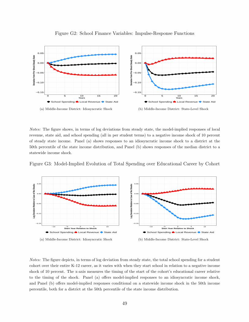
Figure G2: School Finance Variables: Impulse-Response Functions

−0.15

−0.10

−0.05

0.00

0.05

0 5 10 15 20Years

Devia

tion f

rom P

re−Sh

ock S

teady

Stat

e



−0.15

−0.10

−0.05

0.00

0.05

0 5 10 15 20Years

Devia

tion f

rom P

re−Sh

ock S

teady

Stat

e



Notes: The figure shows, in terms of log deviations from steady state, the model-implied responses of local

revenue, state aid, and school spending (all in per student terms) to a negative income shock of 10 percent

of steady state income. Panel (a) shows responses to an idiosyncratic income shock to a district at the

50th percentile of the state income distribution, and Panel (b) shows responses of the median district to a

statewide income shock.

Figure G3: Model-Implied Evolution of Total Spending over Educational Career by Cohort

−0.15

−0.10

−0.05

0.00

0.05


Log D

eviat

ion R

elativ

e to C

ase o

f No S

hock

s



−0.15

−0.10

−0.05

0.00

0.05


Log D

eviat

ion R

elativ

e to C

ase o

f No S

hock

s



Notes: The figure depicts, in terms of log deviation from steady state, the total school spending for a student

cohort over their entire K-12 career, as it varies with when they start school in relation to a negative income

shock of 10 percent. The x-axis measures the timing of the start of the cohort’s educational career relative

to the timing of the shock. Panel (a) offers model-implied responses to an idiosyncratic income shock,

and Panel (b) offers model-implied responses conditional on a statewide income shock in the 50th income

percentile, both for a district at the 50th percentile of the state income distribution.

49

Figure G4: Impulse Responses for i.i.d. Local Income Shocks

−0.03

−0.02

−0.01

0.00

0.01

0 5 10 15 20Years

Devia

tion f

rom P

re−Sh

ock S

teady

Stat

e



−0.04

−0.03

−0.02

−0.01

0.00

0.01

0 5 10 15 20Years

Devia

tion f

rom P

re−Sh

ock S

teady

Stat

e



−0.04

−0.03

−0.02

−0.01

0.00

0.01

0 5 10 15 20Years

Devia

tion f

rom P

re−Sh

ock S

teady

Stat

e



Notes: The figure shows the model implied responses of locally raised revenue, state aid, and school spending (all in log per student terms) to a

negative income shock of 10 percent of steady state local income, assuming an AR parameter for income of 0.

50

Figure G5: Impulse Responses for State-Level i.i.d. Income Shocks

−0.08

−0.04

0.00

0 5 10 15 20Years

Devia

tion f

rom P

re−Sh

ock S

teady

Stat

e



−0.08

−0.04

0.00

0 5 10 15 20Years

Devia

tion f

rom P

re−Sh

ock S

teady

Stat

e



−0.06

−0.03

0.00

0.03

0 5 10 15 20Years

Devia

tion f

rom P

re−Sh

ock S

teady

Stat

e



Notes: The figure shows the model implied responses of local revenue, state aid, and school spending (all in log per student terms) to a negative

income shock of 10 percent of steady state local income that simultaneously affects all school districts, assuming an AR parameter for income of 0.

51

inequality in public school spending across space and time

Documents