inequality constrained minimization logarithmic … program (m = 100 inequalities and n = 50...

Convex Optimization — Boyd & Vandenberghe

12. Interior-point methods

• inequality constrained minimization

• logarithmic barrier function and central path

barrier method • • feasibility and phase I methods

• complexity analysis via self-concordance

• generalized inequalities

12–1

Inequality constrained minimization

minimize f0(x) subject to fi(x) ≤ 0, i = 1, . . . ,m (1)

Ax = b

• fi convex, twice continuously differentiable

• A ∈ Rp×n with rank A = p

⋆ • we assume p is finite and attained

• we assume problem is strictly feasible: there exists x̃ with

x̃ ∈ dom f0, fi(x̃) < 0, i = 1, . . . ,m, Ax̃ = b

hence, strong duality holds and dual optimum is attained

Interior-point methods 12–2

Examples

• LP, QP, QCQP, GP

• entropy maximization with linear inequality constraints

minimize �

in =1 xi log xi

subject to Fx � g Ax = b

with dom f0 = Rn ++

• differentiability may require reformulating the problem, e.g., piecewise-linear minimization or ℓ∞-norm approximation via LP

• SDPs and SOCPs are better handled as problems with generalized inequalities (see later)


Logarithmic barrier

reformulation of (1) via indicator function:

minimize f0(x) + �m

i=1 I−(fi(x)) subject to Ax = b

where I−(u) = 0 if u ≤ 0, I−(u) = ∞ otherwise (indicator function of R−)

approximation via logarithmic barrier

minimize f0(x) − (1/t) �m

log(−fi(x)) i=1 subject to Ax = b

10

• an equality constrained problem 5

• for t > 0, −(1/t) log(−u) is a smooth approximation of I− 0

• approximation improves as t → ∞ −5 −3 −2 −1 0 1

u


�

logarithmic barrier function

m

φ(x) = − log(−fi(x)), dom φ = {x | f1(x) < 0, . . . , fm(x) < 0}i=1

• convex (follows from composition rules)

• twice continuously differentiable, with derivatives

m � 1∇φ(x) = −fi(x)

∇fi(x)i=1

m m � 1 � 1 ∇ 2φ(x) =

fi(x)2 ∇fi(x)∇fi(x)

T + −fi(x)∇ 2fi(x)

i=1 i=1


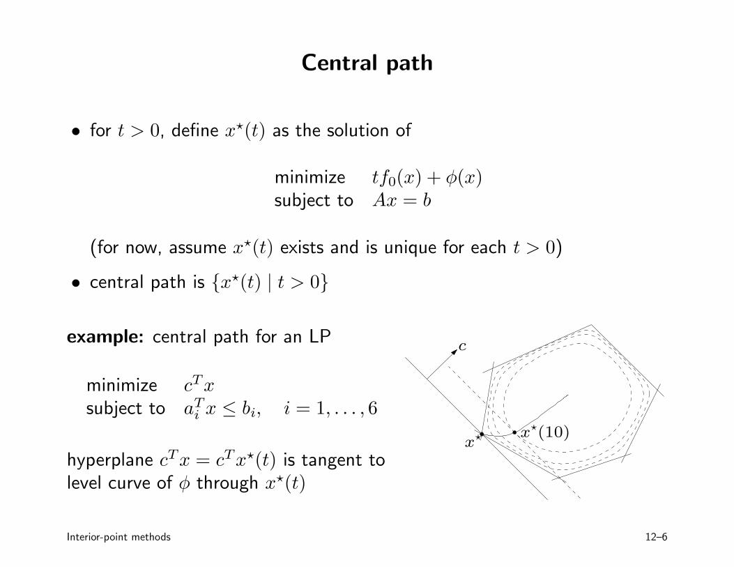
Central path

for t > 0, define x ⋆(t) as the solution of •

minimize tf0(x) + φ(x) subject to Ax = b

(for now, assume x ⋆(t) exists and is unique for each t > 0)

• central path is {x ⋆(t) | t > 0}

example: central path for an LP

⋆ x⋆ (10)

c

minimize cTx subject to ai

Tx ≤ bi, i = 1, . . . , 6

x hyperplane cTx = cTx ⋆(t) is tangent to level curve of φ through x ⋆(t)


�

Dual points on central path

x = x ⋆(t) if there exists a w such that

m

t∇f0(x) + �

−f1

i(x)∇fi(x) +AT w = 0, Ax = b

i=1

therefore, x ⋆(t) minimizes the Lagrangian • m

L(x, λ ⋆ (t), ν ⋆ (t)) = f0(x) + λi⋆ (t)fi(x) + ν ⋆ (t)T (Ax − b)

i=1

where we define λi⋆(t) = 1/(−tfi(x ⋆(t)) and ν⋆(t) = w/t

• this confirms the intuitive idea that f0(x ⋆(t)) → p ⋆ if t → ∞:

p ⋆ ≥ g(λ ⋆ (t), ν ⋆ (t))

= L(x ⋆ (t), λ ⋆ (t), ν ⋆ (t))

= f0(x ⋆ (t)) −m/t


�

Interpretation via KKT conditions

x = x ⋆(t), λ = λ⋆(t), ν = ν⋆(t) satisfy

1. primal constraints: fi(x) ≤ 0, i = 1, . . . ,m, Ax = b

2. dual constraints: λ � 0

3. approximate complementary slackness: −λifi(x) = 1/t, i = 1, . . . ,m

4. gradient of Lagrangian with respect to x vanishes:

m

∇f0(x) + λi∇fi(x) +ATν = 0 i=1

difference with KKT is that condition 3 replaces λifi(x) = 0


�

�

Force field interpretation

centering problem (for problem with no equality constraints)

minimize tf0(x) − m log(−fi(x)) i=1

force field interpretation

• tf0(x) is potential of force field F0(x) = −t∇f0(x) • − log(−fi(x)) is potential of force field Fi(x) = (1/fi(x))∇fi(x)

the forces balance at x ⋆(t):

m

F0(x ⋆ (t)) + Fi(x ⋆ (t)) = 0 i=1


exampleminimize cTx subject to aT

i x ≤ bi, i = 1, . . . ,m

• objective force field is constant: F0(x) = −tc • constraint force field decays as inverse distance to constraint hyperplane:

Fi(x) = −aai

T , �Fi(x)�2 =

dist(

1

x, Hi)bi − i x

where Hi = {x | aiTx = bi}

−c

−3c t = 1 t = 3


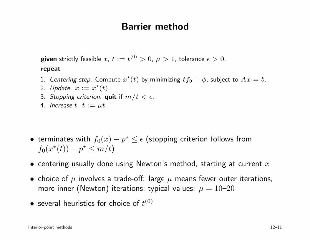
Barrier method

given strictly feasible x, t := t(0) > 0, µ > 1, tolerance ǫ > 0.

repeat

1. Centering step. Compute x⋆ (t) by minimizing tf0 + φ, subject to Ax = b.

2. Update. x := x⋆ (t).

3. Stopping criterion. quit if m/t < ǫ.

4. Increase t. t := µt.

⋆ • terminates with f0(x) − p ≤ ǫ (stopping criterion follows from f0(x ⋆(t)) − p ⋆ ≤ m/t)

• centering usually done using Newton’s method, starting at current x

• choice of µ involves a trade-off: large µ means fewer outer iterations, more inner (Newton) iterations; typical values: µ = 10–20

several heuristics for choice of t(0) •


� �

Convergence analysis

number of outer (centering) iterations: exactly

log(m/(ǫt(0)))

logµ

plus the initial centering step (to compute x ⋆(t(0)))

centering problem

minimize tf0(x) + φ(x)

see convergence analysis of Newton’s method

tf0 + φ must have closed sublevel sets for t ≥ t(0) • • classical analysis requires strong convexity, Lipschitz condition

• analysis via self-concordance requires self-concordance of tf0 + φ


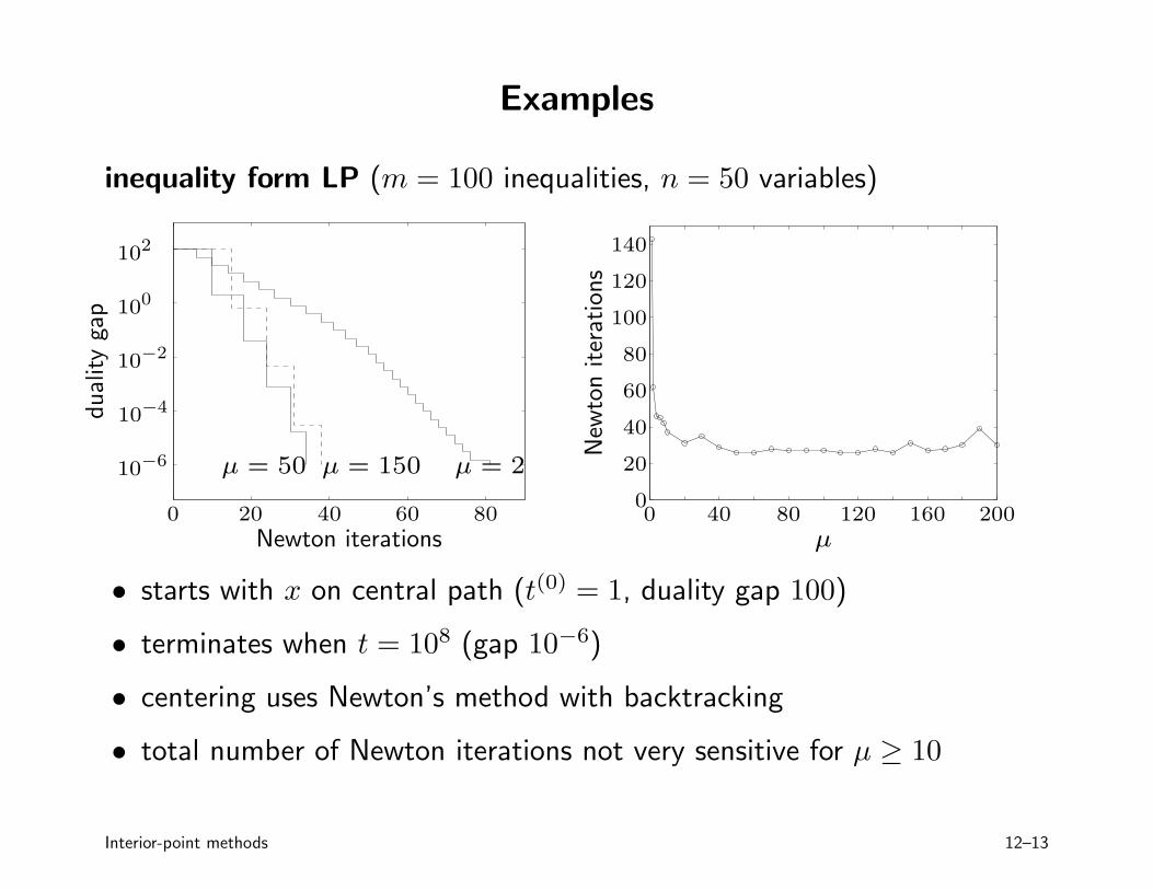
102

Examples

inequality form LP (m = 100 inequalities, n = 50 variables)

140

µ =µ = 50 µ = 150

0 20 40 60 80

10−4

80

0 0 40 80 120 160 200

Newton iterations µ

starts with x on central path (t(0) = 1, duality gap 100)N

ewto

n ite

ration

s •

terminates when t = 108 (gap 10−6)• • centering uses Newton’s method with backtracking

• total number of Newton iterations not very sensitive for µ ≥ 10


120100

dual

ity

gap

100

10−2

60

40

10−6 2 20

� �

� �

geometric program (m = 100 inequalities and n = 50 variables)

�5minimize log k=1 exp(a0

Tkx + b0k)

subject to log �

k5=1 exp(aik

T x + bik) ≤ 0, i = 1, . . . ,m

dual

ity

gap

µ = 2µ = 50 µ = 150 10−6

10−4

10−2

100

102

0 20 40 60 80 100 120Newton iterations


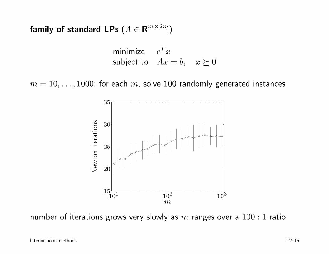
family of standard LPs (A ∈ Rm×2m)

minimize cTx subject to Ax = b, x � 0

m = 10, . . . , 1000; for each m, solve 100 randomly generated instances N

ewto

n ite

ration

s35

30

25

20

15 101 102 103

m

number of iterations grows very slowly as m ranges over a 100 : 1 ratio


Feasibility and phase I methods

feasibility problem: find x such that

fi(x) ≤ 0, i = 1, . . . ,m, Ax = b (2)

phase I: computes strictly feasible starting point for barrier method

basic phase I method

minimize (over x, s) s subject to fi(x) ≤ s, i = 1, . . . ,m (3)

Ax = b

• if x, s feasible, with s < 0, then x is strictly feasible for (2)

⋆ • if optimal value p̄ of (3) is positive, then problem (2) is infeasible

⋆ • if p̄ = 0 and attained, then problem (2) is feasible (but not strictly); ⋆if p̄ = 0 and not attained, then problem (2) is infeasible


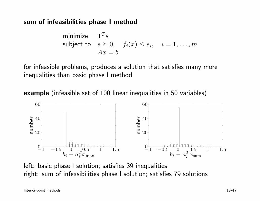
sum of infeasibilities phase I method

minimize 1Ts subject to s � 0, fi(x) ≤ si, i = 1, . . . ,m

Ax = b

for infeasible problems, produces a solution that satisfies many more inequalities than basic phase I method

example (infeasible set of 100 linear inequalities in 50 variables)

60 60

num

ber

40

20 num

ber

40

20

0 0 −1 −0.5 0 0.5 1 1.5 −1 −0.5 0 0.5 1 1.5

bi − aiTxmax bi − ai

Txsum

left: basic phase I solution; satisfies 39 inequalities right: sum of infeasibilities phase I solution; satisfies 79 solutions


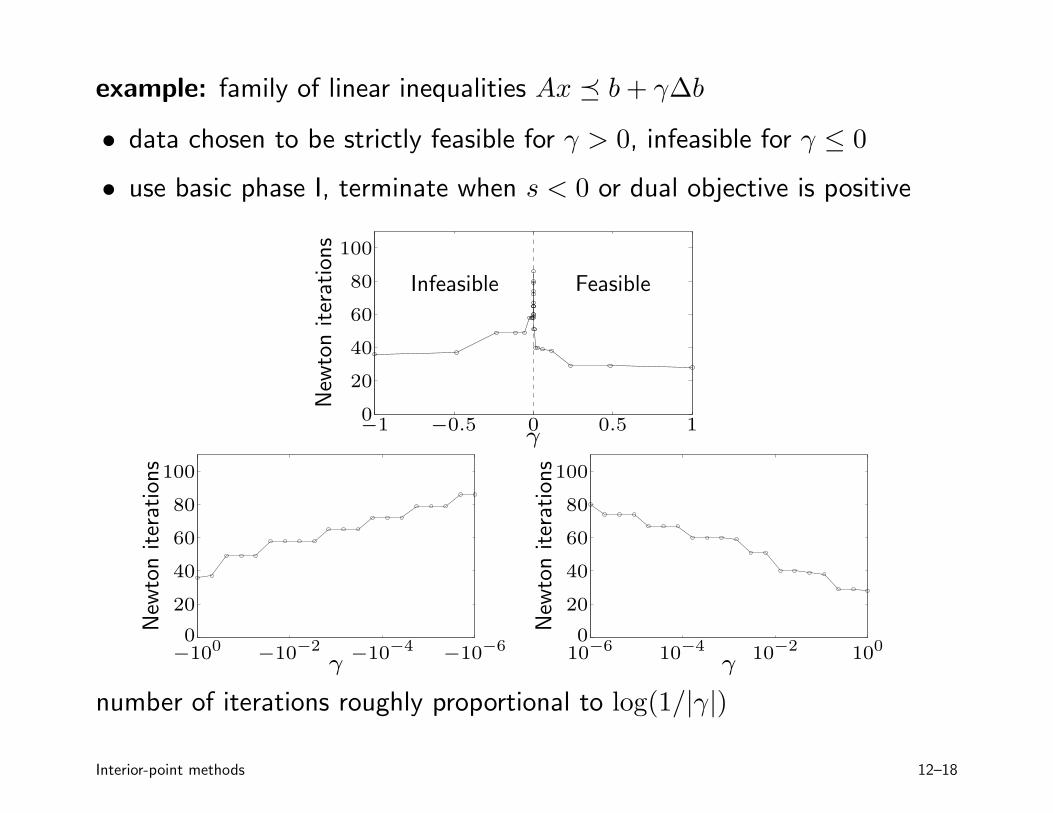
example: family of linear inequalities Ax � b + γΔb

• data chosen to be strictly feasible for γ > 0, infeasible for γ ≤ 0

• use basic phase I, terminate when s < 0 or dual objective is positive

New

ton ite

ration

s

Infeasible Feasible

0

20

40

60

80

100

−1 −0.5 0 0.5 1γ

New

ton ite

ration

s

0

20

40

60

80

100

New

ton ite

ration

s

0

20

40

60

80

100

−100 −10−2

−10−4 −10−6 10−6 10−4 10−2 100

γ γ

number of iterations roughly proportional to log(1/ γ )| |


� �

Complexity analysis via self-concordance

same assumptions as on page 12–2, plus:

• sublevel sets (of f0, on the feasible set) are bounded

• tf0 + φ is self-concordant with closed sublevel sets

second condition

• holds for LP, QP, QCQP

• may require reformulating the problem, e.g.,

minimize in =1 xi log xi minimize i

n =1 xi log xi−→

subject to Fx � g subject to Fx � g, x � 0

• needed for complexity analysis; barrier method works even when self-concordance assumption does not apply


�

�

Newton iterations per centering step: from self-concordance theory

#Newton iterations ≤ µtf0(x) + φ(x) − µtf0(x+) − φ(x+)

+ c γ

bound on effort of computing x+ = x ⋆(µt) starting at x = x ⋆(t)• • γ, c are constants (depend only on Newton algorithm parameters)

from duality (with λ = λ⋆(t), ν = ν⋆(t)): •

µtf0(x) + φ(x) − µtf0(x +) − φ(x +) m

= µtf0(x) − µtf0(x +) + log(−µtλifi(x +)) −m logµ i=1

m

≤ µtf0(x) − µtf0(x +) − µt λifi(x +) −m −m logµ i=1

≤ µtf0(x) − µtg(λ, ν) −m −m log µ

= m(µ − 1 − logµ)


� � � �

total number of Newton iterations (excluding first centering step)

log(m/(t(0)ǫ)) m(µ − 1 − logµ)#Newton iterations ≤ N =

logµ γ + c

N

5 104

4 104

3 104

2 104

1 104

0

figure shows N for typical values of γ, c,

m = 100,m

= 105

t(0)ǫ

1 1.1 1.2µ

• confirms trade-off in choice of µ

• in practice, #iterations is in the tens; not very sensitive for µ ≥ 10


� � ��

polynomial-time complexity of barrier method

for µ = 1 + 1/√m:•

N = O √m log

m/t(0)

ǫ

number of Newton iterations for fixed gap reduction is O(√m)•

• multiply with cost of one Newton iteration (a polynomial function of problem dimensions), to get bound on number of flops

this choice of µ optimizes worst-case complexity; in practice we choose µ fixed (µ = 10, . . . , 20)


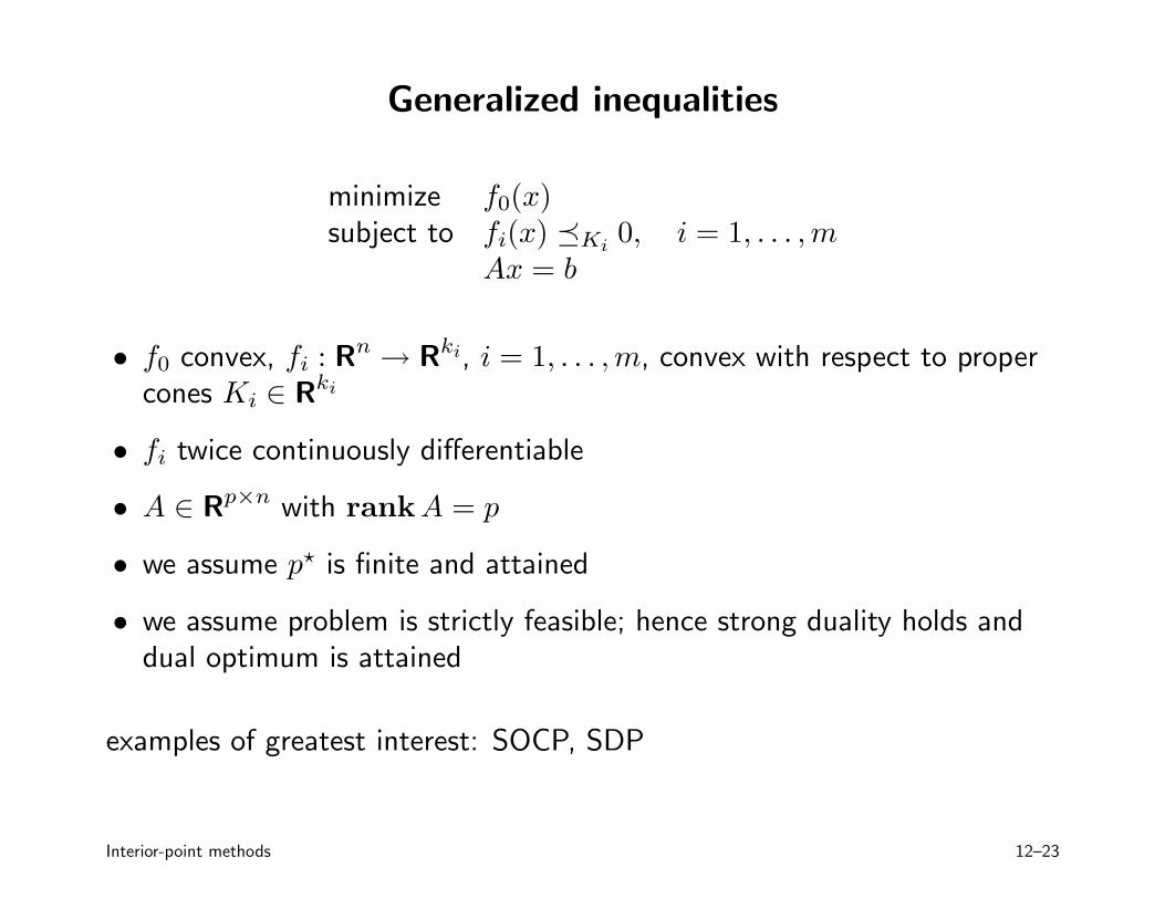
Generalized inequalities

minimize f0(x) subject to fi(x) �Ki

0, i = 1, . . . ,m Ax = b

f0 convex, fi : Rn Rki , i = 1, . . . ,m, convex with respect to proper •

cones Ki ∈ Rki

→

• fi twice continuously differentiable

• A ∈ Rp×n with rank A = p

⋆ • we assume p is finite and attained

• we assume problem is strictly feasible; hence strong duality holds and dual optimum is attained

examples of greatest interest: SOCP, SDP


Generalized logarithm for proper cone

ψ : Rq R is generalized logarithm for proper cone K ⊆ Rq if: →

dom ψ = int K and ∇2ψ(y) ≺ 0 for y ≻K 0• • ψ(sy) = ψ(y) + θ log s for y ≻K 0, s > 0 (θ is the degree of ψ)

examples

nonnegative orthant K = Rn : ψ(y) = �n

log yi, with degree θ = n• + i=1

• positive semidefinite cone K = S+n :

ψ(Y ) = log detY (θ = n)

• second-order cone K = {y ∈ Rn+1 | (y12 + · · · + y2 )1/2 ≤ yn+1}:n

ψ(y) = log(y 2 2 2 ) (θ = 2) n+1 − y1 − · · · − yn


properties (without proof): for y ≻K 0,

∇ψ(y) �K∗ 0, y T ∇ψ(y) = θ

nonnegative orthant Rn : ψ(y) = �n

log yi• + i=1

∇ψ(y) = (1/y1, . . . , 1/yn), y T ∇ψ(y) = n

• positive semidefinite cone S+n : ψ(Y ) = log detY

∇ψ(Y ) = Y −1 , tr(Y ∇ψ(Y )) = n

• second-order cone K = {y ∈ Rn+1 | (y12 + · · · + yn

2 )1/2 ≤ yn+1}:

−.y1

2 ..

T ∇ψ(y) = , y ∇ψ(y) = 2

yn2+1 − y1

2 − · · · − yn 2 −yn

yn+1


�

Logarithmic barrier and central path

logarithmic barrier for f1(x) �K1 0, . . . , fm(x) �Km 0:

m

φ(x) = − ψi(−fi(x)), dom φ = {x | fi(x) ≺Ki 0, i = 1, . . . ,m}

i=1

• ψi is generalized logarithm for Ki, with degree θi

• φ is convex, twice continuously differentiable

central path: {x ⋆(t) | t > 0} where x ⋆(t) solves

minimize tf0(x) + φ(x) subject to Ax = b


�

�

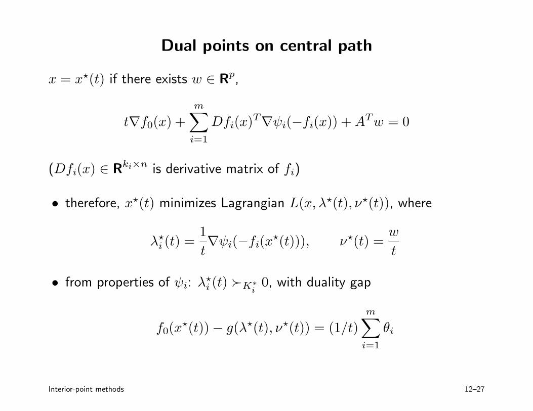
Dual points on central path

x = x ⋆(t) if there exists w ∈ Rp ,

m

t∇f0(x) + Dfi(x)T ∇ψi(−fi(x)) +AT w = 0

i=1

(Dfi(x) ∈ Rki×n is derivative matrix of fi)

therefore, x ⋆(t) minimizes Lagrangian L(x, λ⋆(t), ν⋆(t)), where •

λ ⋆i (t) =1

t ∇ψi(−fi(x ⋆ (t))), ν ⋆ (t) =

w t

from properties of ψi: λ⋆i (t) ≻K∗ 0, with duality gap

i•

m

f0(x ⋆ (t)) − g(λ ⋆ (t), ν ⋆ (t)) = (1/t) θi

i=1


�

example: semidefinite programming (with Fi ∈ Sp)

minimize cTx subject to F (x) = i

n =1 xiFi + G � 0

logarithmic barrier: φ(x) = log det(−F (x)−1)• central path: x ⋆(t) minimizes tcTx − log det(−F (x)); hence •

tci − tr(FiF (x ⋆ (t))−1) = 0, i = 1, . . . , n

dual point on central path: Z⋆(t) = −(1/t)F (x ⋆(t))−1 is feasible for •

maximize tr(GZ) subject to tr(FiZ) + ci = 0, i = 1, . . . , n

Z � 0

duality gap on central path: cTx ⋆(t) − tr(GZ⋆(t)) = p/t •


�

� �

�

Barrier method

given strictly feasible x, t := t(0) > 0, µ > 1, tolerance ǫ > 0.

repeat

1. Centering step. Compute x⋆ (t) by minimizing tf0 + φ, subject to Ax = b. ⋆ 2. Update. x := x (t).

3. Stopping criterion. quit if (P

i θi)/t < ǫ.

4. Increase t. t := µt.

only difference is duality gap m/t on central path is replaced by θi/t • i

number of outer iterations: •

log(( i θi)/(ǫt(0)))

logµ

• complexity analysis via self-concordance applies to SDP, SOCP


102

Examples

second-order cone program (50 variables, 50 SOC constraints in R6)

New

ton ite

ration

s

0

40

80

120 102

dual

ity

gap

100

10−2

10−4

µ = 50 µ = 200 µ =

0 20 40 60 80 20 60 100 140 180 Newton iterations µ

semidefinite program (100 variables, LMI constraint in S100) 140

10−6 2

New

ton ite

ration

s

0 20 40 60 80 100 120

20

60

100100

10−2

10−4

µ =µ = 50 µ = 150

dual

ity

gap

10−6 2

0 20 40 60 80 100 Newton iterations µ


family of SDPs (A ∈ Sn , x ∈ Rn)

minimize 1Tx subject to A + diag(x) � 0

n = 10, . . . , 1000, for each n solve 100 randomly generated instances

New

ton ite

ration

s

35

30

25

20

15 101 102 103

n


Primal-dual interior-point methods

more efficient than barrier method when high accuracy is needed

• update primal and dual variables at each iteration; no distinction between inner and outer iterations

• often exhibit superlinear asymptotic convergence

• search directions can be interpreted as Newton directions for modified KKT conditions

• can start at infeasible points

• cost per iteration same as barrier method


MIT OpenCourseWare http://ocw.mit.edu

6.079 / 6.975 Introduction to Convex Optimization Fall 2009

For information about citing these materials or our Terms of Use, visit: http://ocw.mit.edu/terms.

http://ocw.mit.edu

http://ocw.mit.edu/terms

inequality constrained minimization logarithmic … program (m = 100 inequalities and n = 50...

Documents