industry forecast of demand in china courier - simple...

1

Forecast of Demand in China Courier

Industry

Jiawei Yang

June - 2016

Student thesis, Master degree, 15 HE

Industrial Management Study Program in Industrial Management and Logistics

Supervisor: Muhammad Abid Examiner: Ming Zhao

2

Abstract Since entering 21st century, the courier industry in China has been developing rapidly. In 2016, the revenue of China courier industry accounted for more than 5‰ of China’s GDP. As an emerging industry injected with dynamism and potentials, the courier industry should be integrated into China’s mainstream economy and sustain its growth momentum. The purpose of this thesis is to identify the development trend and demands of the courier industry in China, and provide some suggestions on its future development. The grey model and the regression model were employed as the mathematic techniques in this thesis. First of all, through examining prior literature and availability of related data of China’s courier industry, seven explanatory variables and one explained variable (courier production value) were picked up as the original data. Then, through the use of the grey model, correlations of those seven variables with courier production value are worked out respectively. Third, based on China’s 13th Five-year Plan, three possible GDP growths of 2016 to 2020 (optimistic scenario, negative scenario and normal scenario) were set in this thesis. After that, the future development of seven explanatory variables was reckoned by linear regression model and the assumed GDP growth to predict. Finally, the law of development of explained variable and seven explanatory variables were reckoned by the grey model. Through those result, this thesis drew the conclusions. The result shows that, under three different scenarios, courier industry in China will maintain a tremendous development in the next 5 years. Moreover, all the three main industries (primary industry, secondary industry and tertiary industry) will play important roles in courier industry, among which the tertiary comes first. Also in the coming five years, the development of courier industry, rendering more service to residents, will rely more on the Residents’ consumption and the total retail of goods. And its development will be largely affected by the government’s investment. Another observation concerns total investment in fixed asset which will have a strong impact on the courier industry. That is to say, the government could improve the China courier industry by increasing total investment in fixed asset. Last but not least, the correlation between export-import and courier industry shows that the courier companies should focus more on domestic market.

3

Abstract .............................................................................................................................................2 1 Introduction ...................................................................................................................................5

1.1 Background ..........................................................................................................................5 1.2 Purpose ..................................................................................................................................5 1.3 Limitations ............................................................................................................................6

2 Methodologies ................................................................................................................................7 2.1 Data collection ......................................................................................................................7 2.2 Quantitative Research .........................................................................................................7

2.2.1 The grey model ........................................................................................................8 2.2.2The linear regression model ....................................................................................8

3 Literature review ..........................................................................................................................9 3.1 Definition of supply chain management ............................................................................9 3.2 Logistic management ...........................................................................................................9 3.2.1 Third party logistic (TPL) industry ..............................................................................10 3.3 The evaluation of logistic industry development .............................................................10 3.4 Logistic and Regional economy development ..................................................................11 3.5 Logistics demand forecast .................................................................................................11

4 The current situation of China courier industry .....................................................................12 4.1 The Basic Conditions of Development in Chinese courier Industry ...........................12

4.1.1 Economic gross .....................................................................................................12 4.1.2 The Total retail sales of consumer goods ...........................................................13 4.1.3 Import and export trade ......................................................................................14 4.1.4 Residents consumption ........................................................................................15

4.2 Current situation of China courier industry ................................................................16 4.2.1 The expansion of China courier industry ..........................................................16

5 The variable selection in Chinese courier demand forecast and situation setting ................18 5.1 Correlation analysis of Chinese economy and courier industry .................................18

5.1.1 The selection of dependent variables ..................................................................18 5.1.1.1 The output value of courier industry .......................................................18 5.1.1.2 The output of three main industries ........................................................18 5.1.1.3 The total investment in fixed assets .........................................................18 5.1.1.4 The total retail sales of consumer goods ..................................................19 5.1.1.5 The total export-import volume ...............................................................19 5.1.1.6 The Residents’ consumption ....................................................................19

5.1.2 Research on the correlation of explanatory variables .......................................19 5.1.2.1 The grey correlation model building .......................................................19 5.1.2.2 Calculation of correlation .........................................................................21

5.2 Scenario setting and related data calculation ...............................................................22 5.2.1 Scenario setting ....................................................................................................22 5.2.2 Related data calculation ......................................................................................23 5.2.3 Total value of primary industry ..........................................................................23 5.2.4 The output of secondary industry .......................................................................25 5.2.5 The output of tertiary industry ...........................................................................27 5.2.6 The total investment in fixed assets ....................................................................28

4

5.2.7 The Total retail sales of consumer goods ...........................................................30 5.2.8 The Total export-import volume ........................................................................31 5.2.9 The Residents’ consumption ...............................................................................33 5.2.10 Summary ............................................................................................................34

6 The demand forecast of China courier industry .....................................................................37 6.1 The analysis of demand in China courier industry ......................................................37

6.1.1 Building the grey model .......................................................................................37 6.1.1.1 GM (1, 8) ....................................................................................................37 6.1.1.2 GM (1, 1) ....................................................................................................38

6.1.2 Building China courier demand model ..............................................................39 6.1.3 Building GM (1, 1) model ....................................................................................41

6.1.3.1 GM (1, 1) of the output of primary industry ..........................................41 6.1.3.2 GM (1, 1) of the output of secondary industry .......................................41 6.1.3.3 GM (1, 1) of total value of tertiary industry ...........................................42 6.1.3.4 GM (1, 1) of the total investment in fixed assets .....................................43 6.1.3.5 GM (1, 1) of the Total retail sales of consumer goods ............................43 6.1.3.6 GM (1, 1) of the Total export-import volume .........................................44 6.1.3.7 GM (1, 1) of resident consumption ..........................................................45 6.1.3.8 Forecasting Model of Regional Courier Demand System ......................46 6.1.3.9 Comprehensive prediction model of China courier production value ..47

6.2 Situation Analysis of demand forecast in China courier industry ......................48 6.2.1 Development trend of China courier industry under normal scenario ...48 6.2.2 Development trend of China courier industry under negative scenario .50 6.2.3 Development trend of China courier industry under optimistic scenario ................................................................................................................................51

7 Conclusions .................................................................................................................................53 7.1 Result ...............................................................................................................................53 7.2 Suggestion ........................................................................................................................54

References .....................................................................................................................................55 Journal ...................................................................................................................................55 Book: ......................................................................................................................................56 Website: .................................................................................................................................57

5

1 Introduction The study reported in this thesis aims to show whether the courier industry in China, one of the fastest growing sectors in the country, will maintain its present momentum for growth in next few years. In this introductory chapter, the background and the purpose of the study are introduced and its limitations are explained.

1.1 Background Four years after the Express Mail Service (EMS, one of the mail-service companies in China) started international service in 1980s, it established its domestic express mail service. Later on, the DHL (the world largest logistic company) entered into the Chinese market by cooperating with the Sinotrans (a courier company in China); followed by UPS, FedEx, TNT as well as other less known logistic companies established their presence in China. Led by economic booming in the Pearl River Delta and Yangtze River Delta in the 1990s, domestic courier companies like Shunfeng, Yuantong and Zhongtong made their appearances one after another. In the 21st century, supported by the Chinese government, courier industry has been developing rapidly in China, especially after 2006. The prosperity of e-commerce, facilitating the courier service, speeded up development of the courier industry. With Chinese economy undergoing a rapid transformation, the courier industry plays an increasingly important role in Chinese economic development by bringing much convenience to residents and other businesses, In the future, despite the probable slowdown trend of Chinese economy, improvement of resident consumption and expansion of overseas trades will create a much more flexible environment for Chinese courier industry. The aim of this thesis is to explore the future development trend of Chinese courier industry. And suggestions will be provided for its future development.

1.2 Purpose This thesis aims to propose some guidance for the future development of Chinese courier industry by predicting the demand trend of Chinese courier industry in the future. Courier industry is one of the foundations that ensure the normal operation of national economy, as the development scale of courier industry goes along with the development of economy. Therefore, taking Chinese future economic development as foundation to predict the demand trend of courier industry has guiding significance. Predicting the demand trend of Chinese courier industry is beneficial for the all-round development of courier industry, which will, in turn, benefit China's national economy.

6

1.3 Limitations This study has several limitations. First of all, limited data were used to analyze and predict the overall development trend of Chinese courier industry. Lack of uniform statistical indicator system of courier industry in China has made it harder to acquire related data of e-commerce and courier industry in recent years. Second, empirical studies involving demand forecast of the courier industry has been rather limited, for most of them have focused on logistic instead of courier industry. Third, due to adopting data processing and model application, many parameters needed to be tested and debugged many times to obtain more reliable results. How to find appropriate parameters has been another difficult part of this study. Finally, counting methods have been used in China are different from those used in Europe, which may lead to different units of some statistics.

7

2 Methodologies In order to predict the future demand of courier industry in China, several methods are employed. This chapter gives an overall view of the methods used in this thesis. First, through reading literature on previous studies, several factors (explanatory variables) that may have effects on courier production value (explained variable) were identified. Second, the correlation between those factors and courier production value would be reckoned by adopting grey relational model. Third, three possible GDP growths of China’s 13th Five-year Plan from 2016 to 2020 (optimistic scenario, negative scenario and normal scenario) were set in this thesis, followed by the linear regression model reckoning future development of seven explanatory variables and predict the assumed GDP growth. Meanwhile the correlations between those factors and courier production value in the future are calculated.

2.1 Data collection Walliman (2005) noted that information and statistics are kinds of facts that can be called data, used by researchers to analyze the problems that they intend to investigate. He (2005) also pointed out that there are two different types of methods to collect data: secondary research and primary research. The data used in this thesis is secondary. Remenyi et al (2003) noted that a secondary source would be information already published or available indirectly. Similarly, Walliman (2005) reminded that the source of secondary information would include published articles, books, websites, government departments and commercial bodies. In this thesis all the data is drawn from China Statistical Yearbook, published by Chinese government. Following literature review and availability of related data of China’s courier industry, seven explanatory variables and one explained variable (courier production value) as the original data were selected.

2.2 Quantitative Research The use of mathematical and statistical tools to carry out the analysis of numerical data has long been associated with a more positivistic approach to research (Simon, 2009). Bryman (1988) described quantitative research as being generally underpinned by natural science model. Statistics is the most widely used branch of mathematics in quantitative research. Quantitative research is utilized in this thesis. Large amounts of numerical data were used, and the regression analysis and the grey model were adopted to reach the

8

conclusion.

2.2.1 The grey model The grey model is often used to calculate fuzzy or incomplete data. The main function is to conduct a fuzzy prediction and reveal the possible changing process. The grey model serves well for short-term prediction, for it could work with limited sample but high accuracy. Courier industry, an emerging industry in China, lacks a good statistical indicator system due to data accessibility difficulty. Moreover, courier industry is currently related to a number of other industries (such as railways, navigation etc.), for they all have varying degree of effects on courier industry. Hence, the grey model can work well in this research. In this thesis, the grey model is used to reckon the correlation between several explanatory variables and one explained variable, seeking to find the law of seven explanatory variables and that of explained variable.

2.2.2 The linear regression model The linear regression is an approach for modeling the relationship between a scalar dependent variable Y and one or more explanatory variables (or independent variables) denoted X (David, 2009). Based on original data, it can be an easy task to find the relationship between two variables. The linear regression model and the assumed GDP growth were applied to predict the future development of seven explanatory variables.

9

3 Literature review 3.1 Definition of supply chain management

Supply chain is a system of organizations, people, activities, information, and resources moving a product or service from suppliers to customers. Introduced in 1980’s, supply chain management (SCM) has been drawing increasing attention in last three decades. Definitions about SCM vary by different researches. In Nigel et al (2006)’s book Operation Management, supply chain management is defined as “the management of the interconnection of organizations that relate to each other through upstream and downstream linkages between the processes that produce value to the ultimate consumer in the form of products and services”. They mentioned that all the supply chains share one common and central objective: to satisfy the end customer. Different stages of supply chain should take “end-customer satisfaction” into consideration. It does not matter how far they are from the end-customers. Nigel also listed five objectives that influence the performance of supply chain:

1. Quality. It refers to the quality of products and service that reaches customers. In order to offer end-customers a high quality service, errors need to be avoided in every stage since a small error could invoke a huge loss to end-customers.

2. Speed. Speed is understood from two angles. The first is how fast customers can be served and the second means how quick customers’ demand could be met. In order to have a better performance, supply chain managers should keep both “speed”s run fast.

3. Dependability. Dependability refers to certainty, time in particular. Keeping each process “on-time” is of extreme importance in supply chain, for a small delay during the process could waste more time for end-customers to get their products or services.

4. Flexibility. Supply chain should be flexible enough to cope with changes that may occur during the delivery.

5. Cost. Cost is incurred in each operation. Developments in supply chain management, such as partnership agreements and reduction in the number of suppliers, are all attempts to minimize transaction costs. Nigel et al (2006)’s accounts suggest that the central aim of SCM is to provide a better service to end-customers. And every single unit in the whole supplier chain may exert a huge influence.

3.2 Logistic management Effective logistic management could bring up opportunity for improved profitability and competitive performance (Ballou, 2007). Based on Ballou (2007)’s argument, how to implement an effective logistic management is the main target for those companies intending to improve their logistics. The Council of Supply Chain Management Professionals (2013) defined logistics management as “The procedure of planning, implementing and controlling the

10

effective, cost-efficient flow of goods, storage, work-in-process inventory, finished goods and flow of information from point of origin to point of consumption in order to meet the customer requirements”. With the main objective of adding values, logistics should not only deliver and store goods in the warehouse but also provide more services. Lambert et al (1998) noted that logistics is to ensure the customer service with the lowest logistics costs.

3.2.1 Third party logistic (TPL) industry For different reasons and considerations, companies outsource their logistic process to third party logistic (TPL) companies. TPL is defined extensively in previous articles. Lieb (1992) defined it as “the use of external companies to perform logistics functions that have traditionally been performed within an organization. The functions performed by the third party can encompass the entire logistics process or selected activities within this process”. The definition given by Berglund et al (1999) explained what the logistic process meant for TPL. They said that TPL referred to activities carried out by a logistics service provider on behalf of a shipper and consisting of at least management and execution of transportation and warehousing. In the statement of Bolumole (2003), TPL performs all or part of other companies’ logistic operations. Empirical studies noted that third party logistic is necessary for different business areas at present. Razzaque and Sheng (1998) pointed out that outsourcing of logistics is a business function filled with growing dynamics all over the world. Liu and Lyons (2011) mentioned lacking in logistic abilities in transportation or storage explains why some companies need TPL. However, it is not the only reason why companies choose outsourcing. Armistead (1993) noted another motivation that drives TPL is that companies could focus more on their core competence. On the other hand, certain disadvantages of TPL may come along since companies choose to use TPL service may take the risk of alienating customers (Lonsdale and Cox 2000). The question of improving core competence of TPL remains to be solved for management in most TPL companies. Armistead (1993) advocates that a TPL provider should attach great importance to their quality, speed, dependability and flexibility.

3.3 The evaluation of logistic industry development Research has been conducted to explore the ways of evaluating the logistic industry. Wang (2011) proposed Data Envelopment Analysis (DEA) to evaluate the level of logistic development in some parts of China, finding inadequate investment and inefficiency of human resource in some regions of China. He also worried that an unscientific planning of highway route can be seen in many regions. By adopting grey correlation analysis, Liu and Xie (2011) analyzed the factors that may have influences on logistic industry in Sichuan Province. They found that primary industry

11

produced the strongest influence on logistic industry, followed by tertiary industry, while the secondary industry has the slightest among the three. Zhang and Bao (2005) evaluated locations of logistic centers by building a fuzzy comprehensive evaluation model with the entropy method. 3.4 Logistic and Regional economy development Investigations have been carried out in looking for the relation between logistics, transportation and regional economy. Bolton (1995) indicated a strong relationship between transportation and economy. A prosperous economy must receive substantive support from highly developed traffic, or vice versa. By applying time series analysis and vector auto-regression model on India railways, Mudit (2001) aimed to prove interplay between transportation and economy. Joseph (2003) conducted similar work with Rome as the sample. As for the relationship between logistics and regional economy, researchers vary in their explanations. In Donald (1999)’s research, logistics and regional economy is mutually facilitating and restricting. Basarab (2001) concluded that economy and logistic had a strong relevance after analyzing 42 explanatory factors of logistics performance of a country. Keith (1999) explained the remarkable relationship between regional economies with air transportation in his study.

3.5 Logistics demand forecast Most of logistics demand forecast is based on quantitative method. By using RBF network, Zhou and Wang (2009) built a multivariate nonlinear prediction model, which proves its accuracy despite sample limits, to predict future demand of logistics in Sichuan province. Yan et al (2009), combining Markov model and GM (1, 1) model, predicted the future logistics demand in Shaanxi Province and found that markov model could be a good option on this topic. Chu and Liu (2007) said that at present in China, statistic system of logistic industry needs improvement, and added that GM (1, 1) model is well-suited for data quantizing. Liu (2013) employed generalized regression neural network (GRNN) to predict the logistic demand of Guangdong Province from 2012 to 2015. Compared with other models, GRNN is more suitable for limited and instable sample data. But what is worth mentioning is that most of researchers neglected the current situation of regional economy. Research in other countries is focused more on cargo quantity.

12

4 The current situation of China courier industry

4.1 The Basic Conditions of Development in Chinese courier

Industry

4.1.1 Economic gross The last decade has witnessed high speed growth in Chinese Gross Domestic Product (GDP). As can be seen from figure 4-1, in 2015, China’s GDP totaled 6.7 trillion Yuan. It stands at the second place at that time. It increased by 2.6 times compared with that of 2005. Foreseeing the possible slowdown, China’s economy remains its momentum and grows faster than other countries and regions.

Figure 4-1 Gross Domestic Product from 2005 - 2015（Unit: hundred million Yuan）(Source:

China Statistical Yearbook)

The added value of the secondary industry in China stood at the top among three industries before 2012. But the output of tertiary industry in 2012 reached 2.448 trillion Yuan (Figure 4-2), exceeding the secondary industry. The fast growth of tertiary industry shows that service industry becomes increasingly important in China. As a main content of tertiary industry, courier industry will usher in a rosy prospect.

13

Figure 4-2 The China added value of three main industry（Unit: hundred million Yuan）(Source:

China Statistical Yearbook)

4.1.2 The Total retail sales of consumer goods Consumer market in China is experiencing healthy development. In 2015, the retail sales of consumer goods totaled 30.1 trillion Yuan, up by 10.7% than that of last year (Figure 4-3). And 3.87 trillion Yuan were created from e-commerce, up by 33.3% than that of last year. The growth of the total retail sales of consumer goods slowed down after 2010, but still remained 10% or over per year, a remarkable rise compared with other regions and countries. What’s more, the ever-increasing retail sales online demonstrates that consumers turn to online purchase which stimulates the development of courier industry.

14

Figure 4-3 Chinese the Total retail sales of consumer goods and growth (unit: hundred million

Yuan) (Source: China Statistical Yearbook)

4.1.3 Import and export trade The import and export trade in China developed fast in recent years. The export-import volume in 2014 totaled 4.3 trillion dollar with export of 2.3 trillion and import of 1.9 trillion. Supported by Chinese government, foreign trade volume kept a steady growth since 2005 (Figure 4-4).

15

Figure 4-4 The data of China total export-import volume（unit: million dollars）(Source: China

Statistical Yearbook)

4.1.4 Residents consumption The fast economic growth in China also stimulated rise in resident disposable income. In 2015, the resident consumption averaged 14699 Yuan, with rural consumption at 4941 Yuan and urban, 17104 Yuan. Compared with 2005, the resident consumption increased by almost 3 times. Residents were able to spend more money on purchasing at their disposal. As one of the main channels for resident consumption, online shopping and courier services took this opportunity and experienced fast growth.

16

Table 4-1 The China resident consumption (unit: Yuan) (Source: China Statistical Yearbook)

resident consumption

rural resident consumption

urban resident consumption

2005 5771 2784 9832

2006 6416 3066 10739

2007 7572 3538 12480

2008 8707 4065 14061

2009 9514 4402 15127

2010 10919 4941 17104

2011 13134 6187 19912

2012 14699 6964 21861

2013 16190 7773 23609

2014 17778 8711 25424

4.2 Current situation of China courier industry

4.2.1 The expansion of China courier industry From 2008 to 2015, the average growth rate of China courier revenue is 31.39%, up from 40.8 billion Yuan in 2008 to 276 billion Yuan in 2015. The volume of China courier industry increased from 1.5 billion in 2008 to 20.6 billion in 2015. Three types of courier companies in China market can be found:

1, state – owned courier company, such as Express mail service; 2, private courier company, such as Shunfeng, Shentong, Yuantong;

3, 11foreign courier company, such as Fedex and DHL. Private courier companies have been proportionally large in Chinese market in recent years they, accounting for 86% of total market shares.

17

Figure 4-5 The Production value of China courier industry and growth (Source: China Statistical

Yearbook)

18

5 The variable selection in Chinese courier demand forecast

and situation setting

5.1 Correlation analysis of Chinese economy and courier

industry

5.1.1 The selection of dependent variables Drawing on the convention of selecting dependent variable by previous work and available data of current Chinese courier industry, the output value of courier industry was selected as explained variables and seven variables were regarded as explanatory variables. They are:

1. The output of primary industry; 2. The output of secondary industry; 3. The output of tertiary industry; 4. The total investment in fixed assets; 5. The total retail sales of consumer goods; 6. The total export-import volume; 7. The residents’ consumption.

5.1.1.1 The output value of courier industry Output value of courier industry is one of the most convincing standards used to measure the development of courier industry. It shows the total value of the products and services provided by China courier industry.

5.1.1.2 The output of three main industries All the three important industries in a country would have effects on courier industry in many aspects. Farm products, industrial products and import-export products are all from different industries of national economy. And different industrial structure would create different scale of production, which finally influences the demand of courier industry. It is easy, then, to see that the three main industries would have essential effects on courier industry.

5.1.1.3 The total investment in fixed assets The total investment in fixed assets would influence the courier industry in the

19

following aspects: First, the total investment in fixed assets, improving and remodeling public transportation, such as railway and airport, would enhance the deliver capacity. Second, the total investment in fixed assets expands the public transportation. For instance, building a new airport could help courier industry expand the local market.

5.1.1.4 The total retail sales of consumer goods The total retail sales of consumer goods, as one of the most direct and objective standard, reflect fully the consumer demands. As its name suggests, it shows the total value of consumers’ goods bought by Chinese companies. Consumer goods enter into the market facilitated by courier industry. So it could reflect the demand of courier indirectly. As a service industry, courier would influence the market demand by its cost. In other words, an active demand of market could promote the development of courier industry.

5.1.1.5 The total export-import volume The total export-import volume reflects the commercialization of different regions. Transfer of goods and services ask for strong support from courier industry. A better total export-import volume would enable courier industry to develop fast. In a sense, the total export-import volume and production value of courier industry complement each other.

5.1.1.6 The Residents’ consumption The resident’s consumption reflects the purchasing power of residents. A strong purchasing power would stimulate the related industries and commerce. Just like three main industries, a sound residents’ consumption would promote the development and progress of courier industry.

5.1.2 Research on the correlation of explanatory variables

5.1.2.1 The grey correlation model building As mentioned above, correlation is used to explore the relationship between two or more factors with the change of time. Grey correlation model is often used to describe the correlation among multiple variables. It could find out the degree of synchronization among those variables and then help to reach the conclusions.

20

Here is the derivation of grey correlation model utilized in this thesis： Assuming there are N factors, X1，X2，...，Xn, in a period of time, they would form the sequence｛X1 (t)，X2(t)，...，Xn(t)｝. The correlation formulation of Xi and Xj is：

｛X1 (t)，X2(t)，...，Xn(t)｝, and t=1，2，……m

Hence, at t time, the correlation between Xi and Xj is:

ζij(t)= and t＝1，2，……m △ 𝑚𝑖𝑛 + 𝜎 △ 𝑚𝑎𝑥△ 𝑖𝑗(𝑡) + 𝜎 △ 𝑚𝑎𝑥

Among them, ζij(t) is the correlation coefficient of Xi and Xj at t time, △ij(t) is the absolute value of difference of Xi and Xj at t time (i.e. △ij(t)=丨 Xi — Xj 丨). △min And △max refer to △ij(t) when both Xi and Xj are in maximum or minimum at t time (i.e. △min =mini minj△ij(t)). σ is gray resolution coefficient and . So it can be seen that at period of time, the definition of correlation between Xi and Xj is:

At most of time, equals 0.5. But in this thesis, a more flexible way was used to get gray resolution coefficient. Here is the derivation process:

Set

△ij = , and t=1，2，……m. 1𝑚∑𝑚

𝑡 = 1 △ ij(t)

So we can get:

Set:

Due to σ is among [0,1], so the value of σ(n) is:

1, when ＞3, σ(n)∈[ζij,1.5ζij], under normal circumstance, σ =1.5ζij； 1

ζij

2, when 0＜ ≤3, there will be three different situations: 1

ζij

1, when 2≤ ≤3，σ(n)∈[1.5ζij, 2ζij]most of time, σ(n) =2ζij；; 1

ζij

2, when， 0≤ ＜2，so σ(n) could equals any value among [0.8,1]. 1

ζij

3, when ζij =0, σ(n) could equals to any value among [0, 1].

21

To summarize, after improving the possible value of σ(n), the correlation coefficient of Xi and Xj is:

ζij(t)= , and t＝1，2，……m △ 𝑚𝑖𝑛 + 𝜎(n) △ 𝑚𝑎𝑥△ 𝑖𝑗(𝑡) + 𝜎(𝑛) △ 𝑚𝑎𝑥

5.1.2.2 Calculation of correlation Y as courier production value, X1 is the output of primary industry, X2 is the output of secondary value, X3 is the output of tertiary industry, X4 is total investment of fixed asset, X5 is total retails sales of consumer goods, X6 is the Total export-import volume, and X7 is the Residents’ consumption.

Table 5-1 China economic data(source：China Statistical Yearbook)

Yea

r

Courier

production

value(unit:

billion

Yuan)

The output

of primary

industry(unit

: billion

Yuan)

The output

of

secondary

value(unit:

billion

Yuan)

The

output of

tertiary

industry

(unit:

billion

Yuan)

total

investment of

fixed

asset(unit:

billion Yuan)

total retails

sales of

consumer

goods (unit:

billion

Yuan)

The Total

export-import

volume

(unit: billion

dollar)

The residents’

consumption(unit:

Yuan)

200

8 40.84 3275.32

14995.66

13680.58

17282.8.4

11483.01

17992.147 8707

200

9 47.9 3416.18

16017.17

15474.79

22459.877

13304.82

15064.806 9514

201

0 57.46 3936.26

19162.98

18203.8

25168.377

15800.8 20172.215 10919

201

1 75.8 4616.31

22703.88

21609.86

31148.513

18720.58

23640.199 13134

201

2 105.53

5090.23 24464.3

3 24482.

19 37469.47

4 21443.2

7 24416.021 14699

201

3 151.51

5532.91 26195.6

1 27795.

93 44629.40

9 24284.2

8 25816.889 16190

201

4 204.54

5834.35 27757.1

8 30805.

86 51202.06

5 27189.6

1 26424.177 17778

201

5 276.0 6086.3 27427.8

34156.7

56200.0 30093.1 24574.1 19555.8

Calculation by the grey model reached the correlation of those 7 factors with courier production value (Table 5-2):

22

Table 5-2 The grey correlation of those factors and courier production value

Correlation between primary industry and courier

industry 0.866160824

Correlation between secondary industry and courier

industry 0.857787789

Correlation between tertiary industry and courier

industry 0.82178833

Correlation between total investment of fixed asset

and courier industry 0.764481519

Correlation between retail sales of consumer goods


Correlation between the Total export-import volume


Correlation between the residents’ consumption and

courier industry 0.804763712

As can be seen, the total export-import volume, primary industry and secondary industry have a better correlation than other factors. Meanwhile, total investment of fixed asset has the lowest correlation among those related factors.

5.2 Scenario setting and related data calculation

5.2.1 Scenario setting In this thesis, three possible GDP growths were set, based on the “The 13th Five-year Plan”, initiated by the Chinese government,

Scenario one: normal scenario, based on “The 13th Five-year Plan”, and the GDP growth in the next 5 years in China is expected at 6.5% per year.

Scenario two: Due to a variety of reasons, in the next 5 years, national economy may not grow as fast as expected. Under this circumstance, the growth of GDP was

23

set as 6% per year.

Scenario three: Contrary to scenario two, Chinese economy developed faster than expected. The growth of GDP, thus, is set as 7% per year.

5.2.2 Related data calculation From 2016 to 2020, based on three different predictions of economic growth in China, three different GDP and be figured out:

Table 5-3 China GDP under three different situations（unit：trillion Yuan）

Year 2016 2017 2018 2019 2020

optimistic scenario

72.407756

77.11426014

82.12668705

87.46492171

93.15014162

negative scenario 71.731048

76.39356612

81.35914792

86.64749253

92.27957955

normal scenario 72.069402

76.75391313

81.74291748

87.05620712

92.71486058

Based on this prediction, the linear regression model was adopted to calculate the total output of primary industry, secondary industry, tertiary industry, the total investment in fixed assets, the total retail sales of consumer goods, the total export-import volume, and the residents’ consumption under three situations. As mentioned in methodology section, the linear regression model is presented below.

Yi is called impendent variable, Xi s dependent variable, and β0 is constant；β1 refers to slope. What is worth mentioning is that ui is called error term. Different from mathematical model, ui appeared in economic model which helps to explain the error during measurement or calculation.

5.2.3 Total value of primary industry The data from Table 5-4 was adopted and GDP was set as impendent variable and the output of primary industry was set as dependent variable to build a regression model. This model was then used to predict the output of primary industry under three different situations.

24

Table 5-4 China GDP and The output of primary industry from 2008 to 2015 (unit:

trillion Yuan) (Source: Statistical yearbook of China)

Year GDP The output of primary

industry 2008 31.95155 32.7532

2009 34.90814 34.1618

2010 41.30303 39.3626

2011 48.93006 46.1631

2012 54.03674 50.9023

2013 59.52444 55.3291

2014 64.3974 58.3435

2015 67.6708 60.863

Calculated by Eviews, the result as follow：

Figure 5-1 The result and test of one variable linear regression of the output of primary

industry and GDP T test was given on this regression model at 95 confidences, indicating validity of this one variable linear regression. The goodness of this model (R²) is 0. 997. It can be interpreted that fewer than 95% of confidence, China’s GDP could explain 99.7% of changes of the output of primary industry. The expression of this model is:

25

Combining Table 5-3, this model seeks to calculate the result in three situations (Table 5-5).

Table 5-5 The output of primary industry under three different situations from 2016 to 2020 (unit:

trillion Yuan) Year 2016 2017 2018 2019 2020

optimistic scenario 65.17362 68.99954 73.07414 77.41359 82.03511 negative scenario 64.62353 68.41369 72.45021 76.74910 81.32743 normal scenario 64.89857 68.70661 72.76217 77.08135 81.68127

5.2.4 The output of secondary industry A regression model was made by the data from Table 5-6 and GDP as impendent variable and the output of secondary industry as dependent variable. This model was used to predict the output of secondary industry under three different situations.

Table 5-6 China GDP and The output of secondary industry from 2008 to 2015 (unit: trillion

Yuan) (Source: Statistical yearbook of China)

Year GDP The output of secondary

industry 2008 31.95155 14.99566

2009 34.90814 16.01717

2010 41.30303 19.16298

2011 48.93006 22.70388

2012 54.03674 24.46433

2013 59.52444 26.19561

2014 64.3974 27.75718

2015 67.6708 27.4278

Calculated by Eviews, the result is as follow：

26

Figure 5-2 The result and test of one variable linear regression of the output of secondary

industry and GDP T test was given on this regression model at 95 confidences, indicating validity of this one variable linear regression. The goodness of this model (R²) is 0.977. It can be interpreted that fewer than 95% of confidence, China’s GDP could explain 99.7% of changes of the output of primary industry.

Combining Table 5-3 this model was used to calculate the result in three situations (Table 5-7).

Table 5-7 The output of secondary industry under three different situations from 2016 to 2020

(unit: trillion Yuan) Year 2016 2017 2018 2019 2020


27

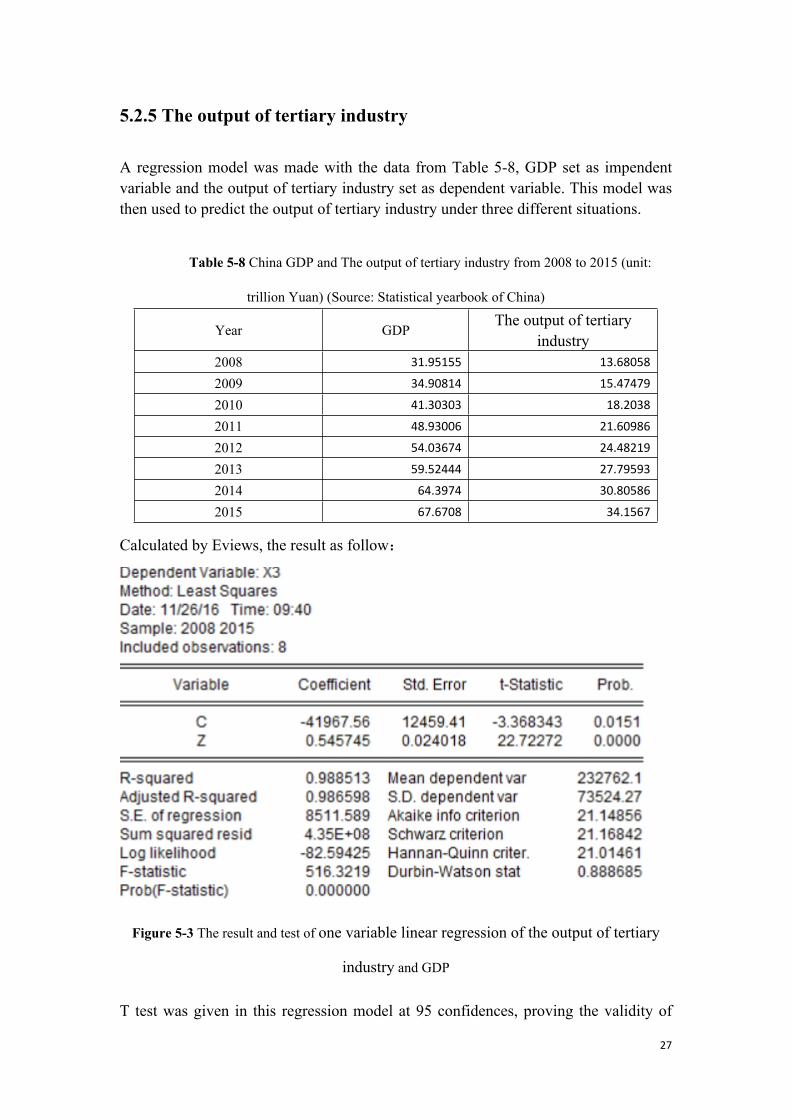
5.2.5 The output of tertiary industry A regression model was made with the data from Table 5-8, GDP set as impendent variable and the output of tertiary industry set as dependent variable. This model was then used to predict the output of tertiary industry under three different situations.

Table 5-8 China GDP and The output of tertiary industry from 2008 to 2015 (unit:

trillion Yuan) (Source: Statistical yearbook of China)

Year GDP The output of tertiary

industry 2008 31.95155 13.68058

2009 34.90814 15.47479

2010 41.30303 18.2038

2011 48.93006 21.60986

2012 54.03674 24.48219

2013 59.52444 27.79593

2014 64.3974 30.80586

2015 67.6708 34.1567


Figure 5-3 The result and test of one variable linear regression of the output of tertiary

industry and GDP T test was given in this regression model at 95 confidences, proving the validity of

28

this one variable. The goodness of this model (R²) is 0. 988. So it can be interpreted that fewer than 95% of confidence, China’s GDP could explain 98.8% of changes of the Total export-import volume. The expression of this model:

Combining Table 5-3 this model seeks to calculate the result in three situations (Table

5-9)

Table 5-9 The output of tertiary industry under three different situations from 2016 to 2020 (unit:

trillion Yuan) Year 2016 2017 2018 2019 2020


5.2.6 The total investment in fixed assets A regression model was made with the data from Table 5-10, GDP set as impendent variable and the total investment in fixed assets set as dependent variable to build a regression model. After that, this model was used to predict the total investment in fixed assets under three different situations.

Table 5-10 China GDP and the total investment in fixed assets from 2008 to 2015 (unit: trillion Yuan) (Source: Statistical yearbook of China)

Year GDP The total investment in

fixed assets 2008 31.95155 17.28284

2009 34.90814 22.459877

2010 41.30303 25.168377

2011 48.93006 31.148513

2012 54.03674 37.469474

2013 59.52444 44.629409

2014 64.3974 51.202065

2015 67.6708 56.2000

29

Calculated by Eviews, the result is as follows：

Figure 5-4 The result and test of one variable linear regression of the total investment in

fixed assets and GDP T test was given in this model at 95 confidences, proving the validity of this one variable. The goodness of this model (R²) is 0.977. It can be interpreted that fewer than 95% of confidence, China’s GDP could explain 97.7% of changes of the total investment in fixed assets. The expression of this model:

So we can combine Table 5-3 and this model to calculate the result in three situations (Table 5-11).

Table 5-11 the total investment in fixed assets under three different situations from 2016 to 2020

(unit: trillion Yuan) Year 2016 2017 2018 2019 2020


30

5.2.7 The Total retail sales of consumer goods A regression model was made with the data from Table 5-12, GDP set as impendent variable and the total retail sales of consumer goods set as dependent variable. This model was used to predict the total retail sales of consumer goods under three different situations.

Table 5-12 China GDP and the Total retail sales of consumer goods from 2008 to 2015

(Unit: trillion Yuan) (Source: Statistical yearbook of China)

Year GDP The Total retail sales of

consumer goods 2008 31.95155 11.48301

2009 34.90814 13.30482

2010 41.30303 15.8008

2011 48.93006 18.72058

2012 54.03674 21.44327

2013 59.52444 24.28428

2014 64.3974 27.18961

2015 67.6708 30.0931


Figure 5-5 the result and test of one variable linear regression of the Total retail sales of

consumer goods and GDP

31

T test was given in this model at 95 confidences, proving the validity of this one variable. The goodness of this model (R²) is 0.988.It can be interpreted that fewer than 95% of confidence, China’s GDP could explain 98.8% of changes of the total retail sales of consumer goods. The expression of this model:

Combining Table 5-3 this model seeks to calculate the result in three situations (Table 5-13).

Table 5-13 The Total retail sales of consumer goods under three different situations from

2016 to 2020 (unit: trillion Yuan) Year 2016 2017 2018 2019 2020


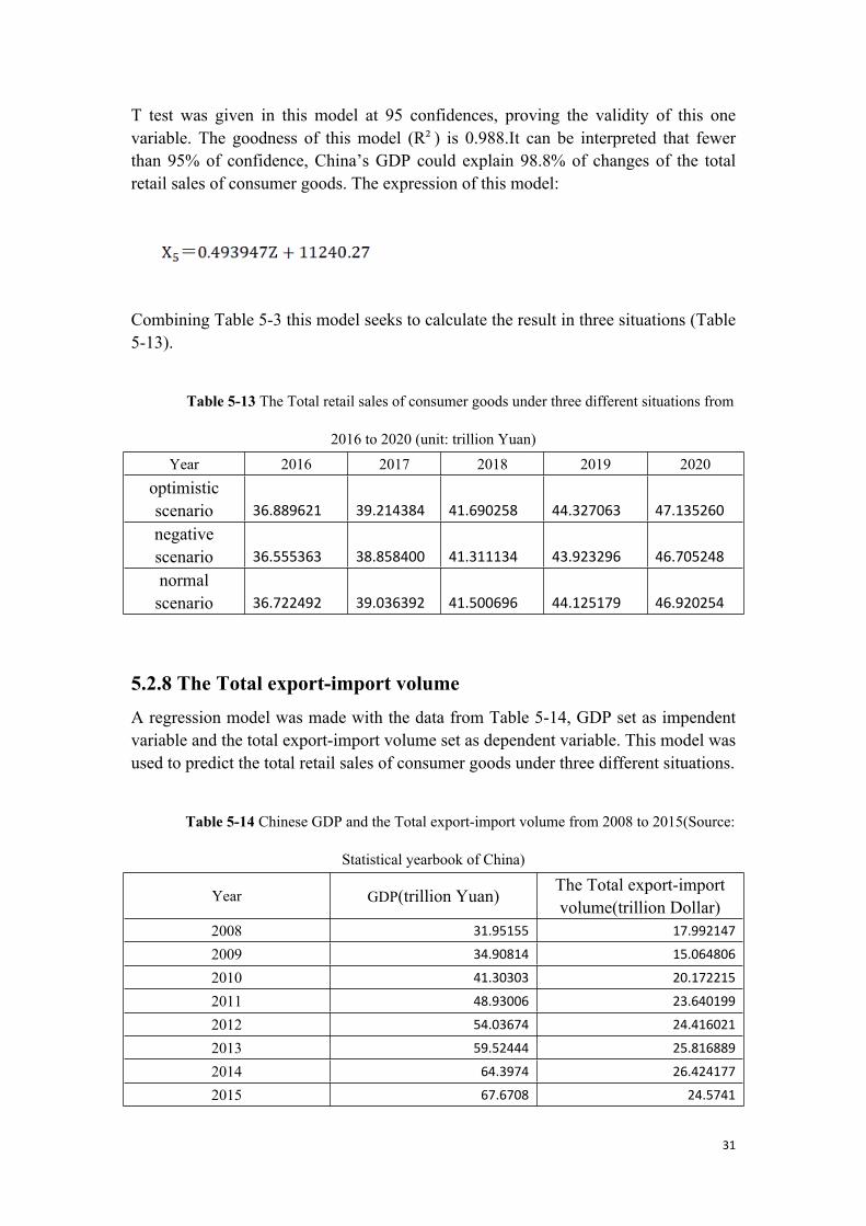
5.2.8 The Total export-import volume A regression model was made with the data from Table 5-14, GDP set as impendent variable and the total export-import volume set as dependent variable. This model was used to predict the total retail sales of consumer goods under three different situations.

Table 5-14 Chinese GDP and the Total export-import volume from 2008 to 2015(Source:

Statistical yearbook of China)

Year GDP(trillion Yuan) The Total export-import volume(trillion Dollar)

2008 31.95155 17.992147

2009 34.90814 15.064806

2010 41.30303 20.172215

2011 48.93006 23.640199

2012 54.03674 24.416021

2013 59.52444 25.816889

2014 64.3974 26.424177

2015 67.6708 24.5741

32


Figure 5-6 the result and test of one variable linear regression of the Total export-import

volume and GDP

T test was given in this model at 95 confidences, proving the validity of this one variable. The goodness of this model (R²) is 0.819. It can be interpreted that fewer than 95% of confidence, China’s GDP of could explain 81.9% of changes of the total export-import volume. The expression of this model:

Combing Table 5-3, this model seeks to calculate the result in three situations (Table 5-15).

Table 5-15 The Total export-import volume under three different situations from 2016 to 2020

(unit: trillion Dollars) Year 2016 2017 2018 2019 2020


33

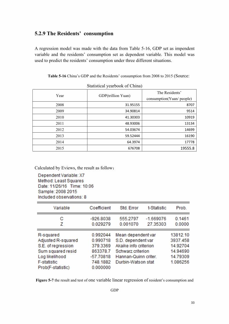
5.2.9 The Residents’ consumption A regression model was made with the data from Table 5-16, GDP set as impendent variable and the residents’ consumption set as dependent variable. This model was used to predict the residents’ consumption under three different situations.

Table 5-16 China’s GDP and the Residents’ consumption from 2008 to 2015 (Source:

Statistical yearbook of China)

Year GDP(trillion Yuan) The Residents’

consumption(Yuan/ people) 2008 31.95155 8707

2009 34.90814 9514

2010 41.30303 10919

2011 48.93006 13134

2012 54.03674 14699

2013 59.52444 16190

2014 64.3974 17778

2015 676708 19555.8


Figure 5-7 the result and test of one variable linear regression of resident’s consumption and

GDP

34

T test was given in this model at 95 confidences, proving the validity of this one variable. The goodness of this model (R²) is 0.992.It can be interpreted that fewer than 95% of confidence, China’s GDP could explain 99.2% of changes of resident’s consumption. The expression of this model:

Combining Table 5-3, this model seeks to calculate the result in three situations

(Table 5-17).

Table 5-17 The Residents’ consumption under three different situations from 2016 to 2020

(Yuan/people) Year 2016 2017 2018 2019 2020


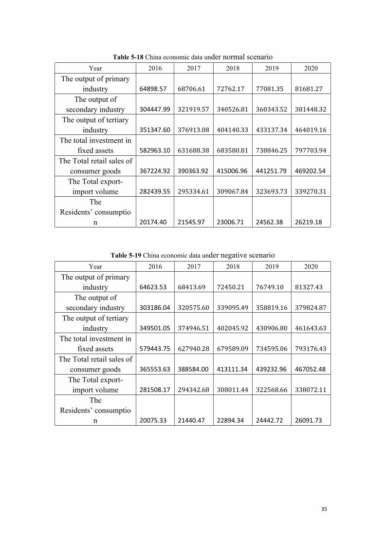
5.2.10 Summary All the results achieved above would help to calculate the output of primary industry, secondary industry, tertiary industry, the total investment in fixed assets, the Total retail sales of consumer goods, the Total export-import volume, and the Residents’ consumption under three different situations.

35

Table 5-18 China economic data under normal scenario Year 2016 2017 2018 2019 2020

The output of primary industry 64898.57 68706.61 72762.17 77081.35 81681.27

The output of secondary industry 304447.99 321919.57 340526.81 360343.52 381448.32

The output of tertiary industry 351347.60 376913.08 404140.33 433137.34 464019.16

The total investment in fixed assets 582963.10 631688.38 683580.81 738846.25 797703.94

The Total retail sales of consumer goods 367224.92 390363.92 415006.96 441251.79 469202.54

The Total export-import volume 282439.55 295334.61 309067.84 323693.73 339270.31

The Residents’ consumptio

n 20174.40 21545.97 23006.71 24562.38 26219.18

Table 5-19 China economic data under negative scenario Year 2016 2017 2018 2019 2020








n 20075.33 21440.47 22894.34 24442.72 26091.73

36

Table 5-20 China economic data under optimistic scenario Year 2016 2017 2018 2019 2020








n 20273.46 21651.48 23119.07 24682.05 26346.63

37

6 The demand forecast of China courier industry

6.1 The analysis of demand in China courier industry

6.1.1 Building the grey model In general, there are two ways to calculate the GM model, and they are accumulated generating operation and accumulated reduction operation. As their name suggest, accumulated generating operation would make sequences plus together to obtain new sequence and data:

On the contrary, accumulated reduction operation would make sequences minus together to obtain new sequence and data:

In this thesis, accumulated generating operation to calculate and process data were used.

6.1.1.1 GM (1, 8) In this thesis, 8 factors were mentioned. A GM (1, 8) was built to find the relationship between them; the differential equation is as follows:

And

After calculating the equation:

38

6.1.1.2 GM (1, 1) Also, GM (1, 1) is used to test the precision of those factors. In other words, the purpose of GM (1, 1) is to test whether those predicted data is reasonable. The differential equation is as follows:

And

After calculating the equation:

Posterior error is used to test the precision of model in this thesis (table 6-1), and the following table demonstrates the accuracy standard of posterior error of the grey model (Ning et al, 2009):

Table 6-1 The standard of Posterior error

Good Fair Barely qualified Unqualified

P (minimum error

probability)

C (variance ration)

39

6.1.2 Building China courier demand model

Based on the variables set on chapter 4, Y equals the output value of courier industry, X1 is The output of primary industry, X2 for secondary industry, X3 for tertiary industry, X4 for the total investment in fixed assets, X5 for the total retail sales of consumer goods, X6 equals to the total export-import volume and X7 means the Residents’ consumption. And the related data from 2008 to 2015 was used as well (Table 6-2).

Table 6-2 The related data of China’s economy (Source: Statistical yearbook of China)

Year

The

output

value of

courier

industry

（billion

Yuan）

The

output of

primary

industry

(trillion

Yuan)

The

output of

secondar

y

industry

(trillion

Yuan)

The

output of

tertiary

industry

(trillion

Yuan)

The

total

invest

ment

in

fixed

assets(

trillion

Yuan)

The Total

retail sales

of

consumer

goods(trilli

on Yuan)

The Total

export-import

volume

（trillion

dollar）

The

Residents’ co

nsumption

（Yuan/peop

le）

2008 40.84

32.7532 14.9956

6 13.6805

8 17.28284

11.48301 17.992147 8707

2009 47.9

34.1618 16.0171

7 15.4747

9 22.459877

13.30482 15.064806 9514

2010 57.46

39.3626 19.1629

8 18.2038

25.168377

15.8008 20.172215 10919

2011 75.8

46.1631 22.7038

8 21.6098

6 31.148513

18.72058 23.640199 13134

2012 105.53

50.9023 24.4643

3 24.4821

9 37.469474

21.44327 24.416021 14699

2013 151.51

55.3291 26.1956

1 27.7959

3 44.629409

24.28428 25.816889 16190

2014 204.54

58.3435 27.7571

8 30.8058

6 51.202065

27.18961 26.424177 17778

2015 276

60.863 27.4278 34.1567 56.20

00 30.0931 24.5741

19555.8

Original sequences as follow：

Y(0) ={408.4 479 574.6 758 1055.3 1515.1 2045.4 2760} X1

(0) ={32753.2 34161.8 39362.6 46163.1 50902.3 55329.1 58343.5 60863}

40

X2(0) ={149956.6 160171.7 191629.8 227038.8 244643.3 261956.1

277571.8 274278} X3

(0) ={136805.8 154747.9 182038 216098.6 244821.9 277959.3 308058.6 341567}

X4

(0) ={172828.4 224598.77 251683.77 311485.13 374694.74 446294.09 512020.65 562000}

X5

(0) ={114830.1 133048.2 158008 187205.8 214432.7 242842.8 271896.1 300931}

X6

(0) ={179921.47 150648.06 201722.15 236401.99 244160.21 258168.89 264241.77 245741}

X7

(0) ={8707 9514 10919 13134 14699 16190 17778 19555.8} Sequence after once accumulated: Y(1)={408.4 887.4 1462 2220 3275.3 4790.4 6835.8 9595.8} X1

(1) ={32753.2 66915.00 106277.60 152440.70 203343.00 258672.10 317015.60 377878.60}

X2

(1) ={ 149956.6 310128.30 501758.10 728796.90 973440.20 1235396.30 1512968.10 1787246.10}

X3

(1) ={ 136805.8 291553.70 473591.70 689690.30 934512.20 1212471.50 1520530.10 1862097.10}

X4

(1) ={172828.4 397427.17 649110.94 960596.07 1335290.81 1781584.90 2293605.55 2855605.55}

X5

(1) ={114830.1 247878.30 405886.30 593092.10 807524.80 1050367.60 1322263.70 1623194.70}

X6

(1) ={179921.47 330569.53 532291.68 768693.67 1012853.88 1271022.77 1535264.54 1781005.54}

X6

(1) ={8707 18221.00 29140.00 42274.00 56973.00 73163.00 90941.00 110496.80}

41

6.1.3 Building GM (1, 1) model Because the output of primary industry, secondary industry, tertiary industry, the total investment in fixed assets, the total retail sales of consumer goods, and the total export-import volume and means the Residents’ consumption are all independent variables, 7 GM (1, 1) models were built to test the precision of the model.

6.1.3.1 GM (1, 1) of the output of primary industry

The B and Y matrix of total value of primary industry in GM (1, 1):

B = , Y = [ ‒ 49834.1 1‒ 86596.3 1

‒ 129359.15 1‒ 177891.85 1‒ 231007.55 1‒ 287853.85 1‒ 347447.1 1

] [34161.839362.646163.150902.355329.158343.560863

]Matlab led to A

So GM (1, 1) model of total value of primary industry is:

The posterior error of this model:

The result shows the suitability of the model in that the posterior error was more than

0.8.

6.1.3.2 GM (1, 1) of the output of secondary industry

The B and Y matrix of total value of secondary industry in GM (1, 1):

42

B = , Y = [ ‒ 230042.45 1‒ 405943.20 1‒ 615277.50 1‒ 851118.55 1

‒ 1104418.25 1‒ 1374182.20 1‒ 1650107.10 1

] [160171.7191629.8227038.8244643.3261956.1277571.8274278

]The Matlab led to A.

So GM (1, 1) model of total value of secondary industry is:



0.8.

6.1.3.3 GM (1, 1) of total value of tertiary industry The B and Y matrix of total value of tertiary industry in GM (1, 1):

, Y = [154747.9182038

216098.6244821.9277959.3308058.6341567


So GM (1, 1) model of total value of tertiary industry is:


43

The result shows the suitability of the model in that the posterior error was more than 0.95.

6.1.3.4 GM (1, 1) of the total investment in fixed assets The B and Y matrix of total investment in fixed asset in GM (1, 1):

, Y = [224598.77251683.77311485.13374694.74446294.09512020.65

562000]

The Matlab led to A.

So GM (1, 1) model of total investment in fixed asset is:



6.1.3.5 GM (1, 1) of the Total retail sales of consumer goods

The B and Y matrix of the Total retail sales of consumer goods in GM (1, 1):

, Y = [133048.2158008

187205.8214432.7242842.8271896.1300931


So GM (1, 1) model of the Total retail sales of consumer goods is:

44



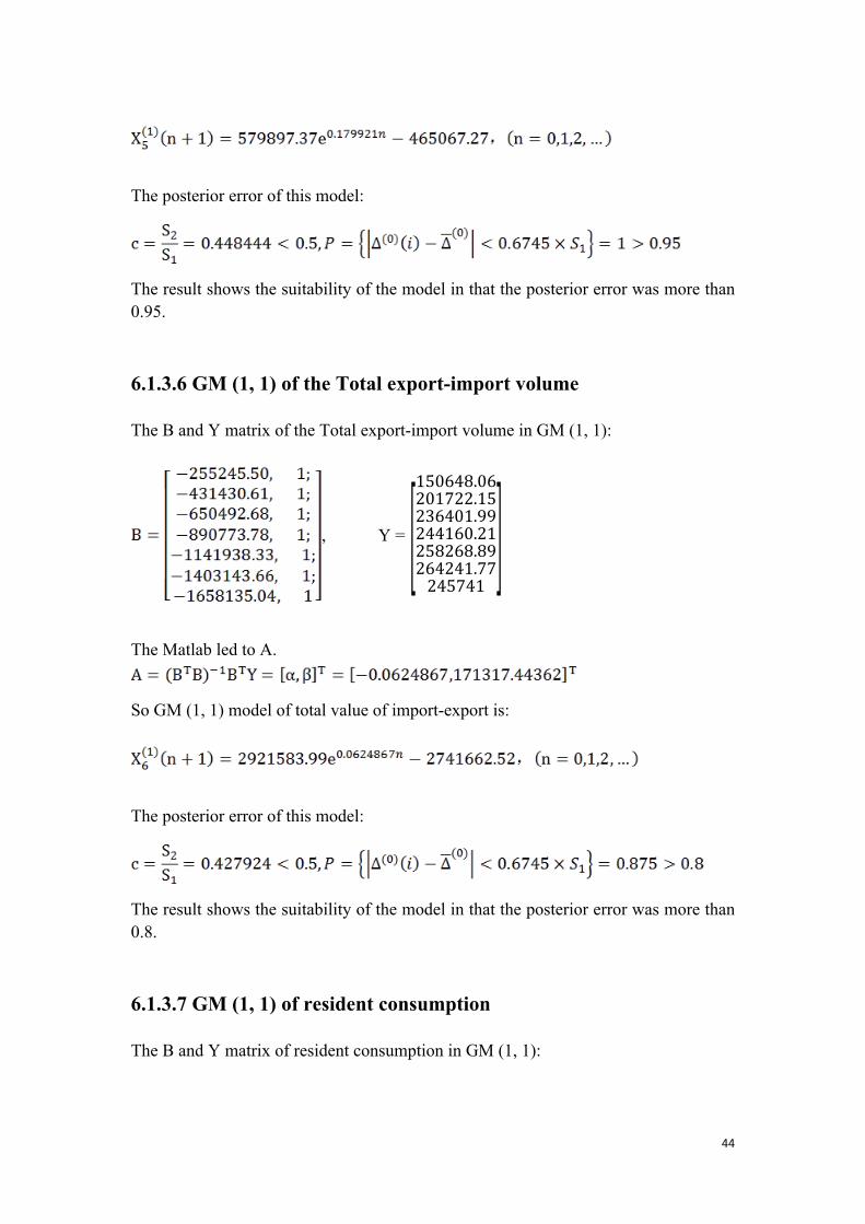
6.1.3.6 GM (1, 1) of the Total export-import volume

The B and Y matrix of the Total export-import volume in GM (1, 1):

, Y = [150648.06201722.15236401.99244160.21258268.89264241.77

245741]


So GM (1, 1) model of total value of import-export is:



6.1.3.7 GM (1, 1) of resident consumption

The B and Y matrix of resident consumption in GM (1, 1):

45

, Y = [ 951410919

131314146991619017778

19555.8]


So GM (1, 1) model of resident consumption is:



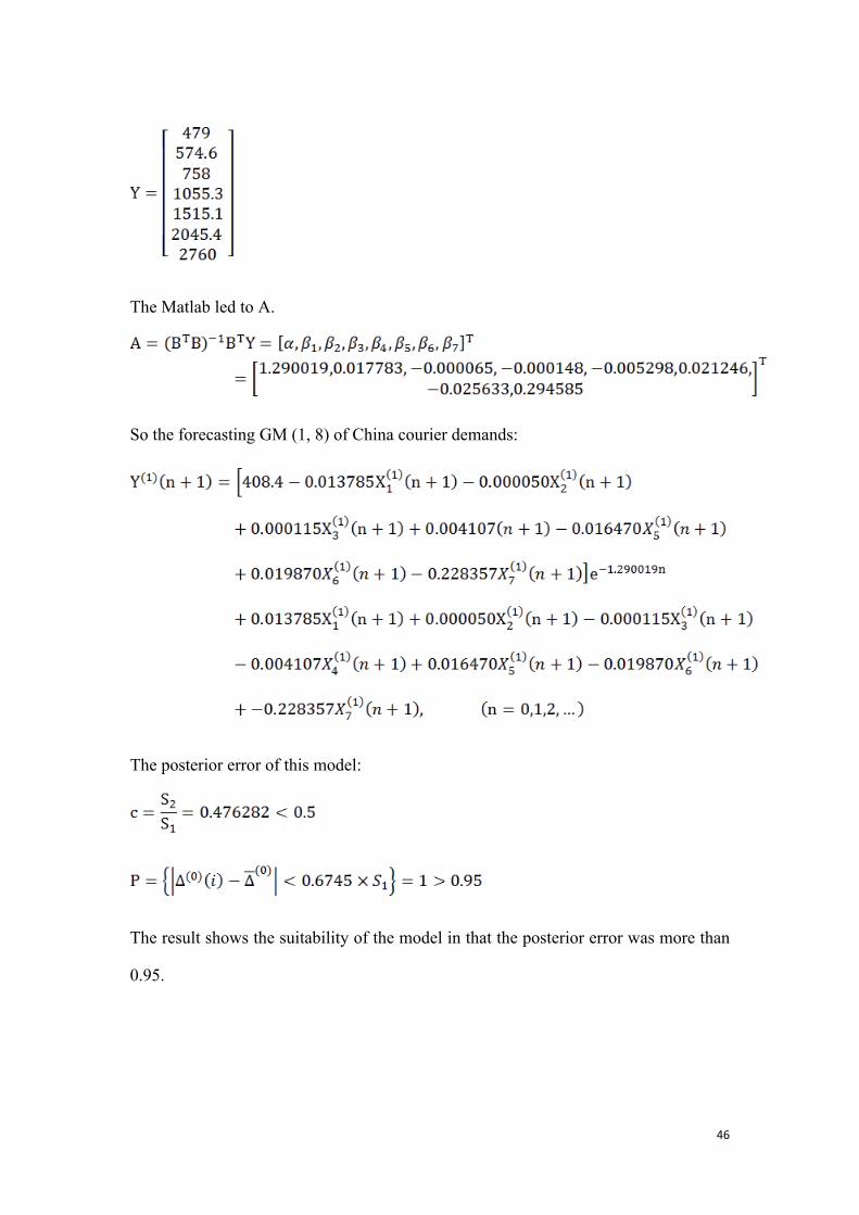
6.1.3.8 Forecasting Model of Regional Courier Demand System Before building the forecasting model of regional courier demand system, GM (1, 8) of regional courier demand was built.

= {408.4 887.4 1462 2220 3275.3 4790.4 6835.8 9595.8}

= {408.4 479 574.6 758 1055.3 1515.1 2045.4 2760}

The B and Y matrix of GM (1, 1) of region courier demand:

46


So the forecasting GM (1, 8) of China courier demands:



0.95.

47

6.1.3.9 Comprehensive prediction model of China courier production

value Based on the above analysis and calculation, the GM (1, 1) of total value of primary industry, secondary industry, tertiary industry, total investment in fixed asset, the total retail sales of consumer goods, the total export-import volume and the Residents’ consumption and GM (1, 8) of forecast of China courier production value were obtained. A comprehensive model of China courier production value was established, which is used to predict the China courier production value in the next few years. The model is as follows:

Moreover, as proved above, the precision of those 8 models has a high accuracy. This comprehensive model is suitable for prediction and analysis.

6.2 Situation Analysis of demand forecast in China courier industry The model displayed the courier demand in different situations in the next 5 years.

48

6.2.1 Development trend of China courier industry under normal

scenario Under normal scenario, from 2016 to 2020, economic growth in China will stay at a speed of 6.5% per year (Table 6-2).

Table 6-2 China courier production value from 2016 to 2020 under normal scenario (unit: billion Yuan)

Year 2016 2017 2018 2019 2020

China courier

production value 351.827 380.669 411.384 444.095 478.931

Data based on the courier demand shows that when economy grows at 6.5% per year, the courier revenue would rise up in the next 5 years. As Table 6-2 shows, the growth rate is 27.47%、8.19%、8.07%、7.95%、7.84% respectively. Combing the other economic data under normal scenario, the correlation coefficient matrix and grey correlation between courier production value and other economic data were reckoned (Table 6-4):

Table 6-4 grey correlation between courier production value and other economic data

Correlation between courier production and primary industry 0.931087

Correlation between courier production and secondary industry

0.931332

Correlation between courier production and tertiary industry 0.916074

Correlation between courier production and total investment in fixed asset 0.906057

Correlation between courier production and the Total retail sales of consumer goods 0.925579

Correlation between courier production and the Total export-import volume 0.943860

Correlation between courier production and The Residents’ consumption 0.923409

Comparison with Table 5-2 led to some findings. Table 5-2 indicated that the primary industry and the total export-import volume has the best synchronization to courier production value among those explanatory variables (relevancy is higher than 86%). in Table 6-3, the relevancy of those 7 variables exceeds 90%.

49

Moreover, it can be seen that the correlation of primary industry, total investment in fixed asset, the total retail sales of consumer goods and the Residents’ consumption had more tremendous correlation than before. Tertiary industry and the Residents’ consumption keep a steady correlation with courier industry.

6.2.2 Development trend of China courier industry under negative

scenario Under normal scenario, from 2016 to 2020, economy in China will grow at a speed of 6% per year (Table 6-5).

Table 6-5 China courier production value from 2016 to 2020 under negative

scenario (unit: billion Yuan)

Year 2016 2017 2018 2019 2020

China courier


Data based on the courier demand shows that when economy grows at 6.5% per year, the courier revenue would rise up in the next 5 years. As Table 6-4 shows, the growth rate is 28.23%、8.19%、8.06%、7.94%、7.84% respectively. Combing the other economic data under normal scenario, the correlation coefficient matrix and grey correlation between courier production value and other economic data were reckoned (Table 6-6):

50

Table 6-6 Grey correlation between courier production value and other economic data Correlation between courier production and primary

industry 0.931119 Correlation between courier production and

secondary industry 0.931366 Correlation between courier production and tertiary

industry 0.916035 Correlation between courier production and total

investment in fixed asset 0.905956 Correlation between courier production and the

Total retail sales of consumer goods 0.925589 Correlation between courier production and the

Total export-import volume 0.943931 Correlation between courier production and The

Residents’ consumption 0.923409


Moreover, it can be seen that the correlation of primary industry, total investment in fixed asset, the total retail sales of consumer goods and the Residents’ consumption had more tremendous correlation than before. Tertiary industry and the Residents’ consumption keep a steady correlation with courier industry.

6.2.3 Development trend of China courier industry under optimistic

scenario Under normal scenario, from 2016 to 2020, economy in China will grow at a speed of 7% per year (Table 6-7).

51

Table 6-7 China courier production value from 2016 to 2020 under optimistic

scenario (unit: billion Yuan)

Year 2016 2017 2018 2019 2020

China courier


Data based on the courier demand shows that when economy grows at 7% per year, the courier revenue would rise up in the next 5 years. As Table 6-6 shows, the growth rate is 26.72%、8.21%、8.08%、7.96%、7.86% respectively. Combing the other economic data under normal scenario, the correlation coefficient matrix and grey correlation between courier production value and other economic data were reckoned (Table 6-8):

Table 6-8 Grey correlation between courier production value and other economic data

Correlation between courier production and primary industry 0.931055

Correlation between courier production and secondary industry 0.931299

Correlation between courier production and tertiary industry 0.916111

Correlation between courier production and total investment in fixed asset 0.906157

Correlation between courier production and the Total retail sales of consumer goods 0.925569

Correlation between courier production and the Total export-import volume 0.943790

Correlation between courier production and the Residents’ consumption 0.923409


Moreover, it can be seen that the correlation of primary industry, total investment in fixed asset, the total retail sales of consumer goods and the Residents’ consumption had more tremendous correlation than before. Tertiary industry and the Residents’ consumption keep a steady correlation with courier industry

52

7 Conclusions

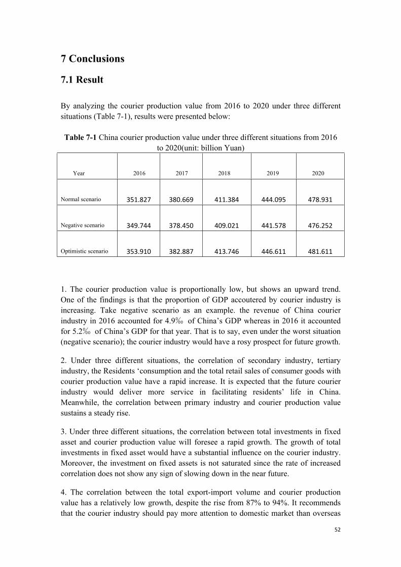
7.1 Result By analyzing the courier production value from 2016 to 2020 under three different situations (Table 7-1), results were presented below: Table 7-1 China courier production value under three different situations from 2016

to 2020(unit: billion Yuan)

Year 2016 2017 2018 2019 2020

Normal scenario 351.827 380.669 411.384 444.095 478.931

Negative scenario 349.744 378.450 409.021 441.578 476.252

Optimistic scenario 353.910 382.887 413.746 446.611 481.611

1. The courier production value is proportionally low, but shows an upward trend. One of the findings is that the proportion of GDP accoutered by courier industry is increasing. Take negative scenario as an example. the revenue of China courier industry in 2016 accounted for 4.9‰ of China’s GDP whereas in 2016 it accounted for 5.2‰ of China’s GDP for that year. That is to say, even under the worst situation (negative scenario); the courier industry would have a rosy prospect for future growth.

2. Under three different situations, the correlation of secondary industry, tertiary industry, the Residents ‘consumption and the total retail sales of consumer goods with courier production value have a rapid increase. It is expected that the future courier industry would deliver more service in facilitating residents’ life in China. Meanwhile, the correlation between primary industry and courier production value sustains a steady rise.

3. Under three different situations, the correlation between total investments in fixed asset and courier production value will foresee a rapid growth. The growth of total investments in fixed asset would have a substantial influence on the courier industry. Moreover, the investment on fixed assets is not saturated since the rate of increased correlation does not show any sign of slowing down in the near future.

4. The correlation between the total export-import volume and courier production value has a relatively low growth, despite the rise from 87% to 94%. It recommends that the courier industry should pay more attention to domestic market than overseas

53

market.

7.2 Suggestion

Several suggestions are proposed in this thesis based on a comprehensive analysis of the correlations in the previous chapters.

1. It is reasonable to hold out the possibility that courier services, playing an increasingly important role in national economy, would penetrate into people’s daily life to a fuller extent. The future development of courier industry will depend on the total investment in fixed assets, increase of which from the Chinese government will contribute to the future growth of the courier industry.

2. The correlation of courier productions and three main industries exceeds 90% in 2020. Courier services will not only enter into people’s life but also give itself a full play in agriculture and industry. Courier service network should be improved by the Chinese government in both industrial and agricultural districts instead of exclusive focus on urban areas.

3. Cooperation between courier industry and retail trade shall be strengthened. As one of the main supports of courier industry, retail trade is expected to cooperate with courier companies. Despite the prominent role played by courier industry to three main industries and the over 90% correlation of courier productions and primary and secondary industries, the relationship between the Residents ‘consumption cannot be neglected. In other words, developing residents ‘consumptions means more than developing industrial districts and agricultural districts

4. Courier resources should be integrated. The courier industry, as the research has shown, will not remain as a small industry anymore. It is undergoing rapid development and has close relationship with other industries. The courier industry should develop in a down-to-earth manner and evolve from traditional courier industry to a diversified one.

54

References

Journal

Armistead, C.G. and Mapes, J (1993). The impact of supply chain integration on operation performance. Logistics information management 6(1): 9-14

Ballou, R. H. (2007). The evolution and future of logistics and supply chain management. European Business Review 19(4): 332 – 348

Berglund, M., Van Laarhoven, P., Sharman, G., and Wandel, S. (1999). Third-party logistics: is there a future? The International Journal of Logistics Management 10(1): 59-70

Bolumole, Y.A. (2003). Evaluating the Supply Chain Role of Logistics Service Providers. The International Journal of Logistics Management 14(2): 93- 107.

Basarab (2008). An analysis of explanatory factors of logistics performance of a country, The logistics of merchandise 10(24):143-156.

Chris Lonsdale and Andrew Cox (2000). The historical development of outsourcing: the latest fad? Industrial Management & Data Systems 100(9):444 – 450

Chu Yf and Liu Sf (2008). Research on the development of logistics in China based on Grey System Theory. Management review 3(1):58-62

Keith G Debbage (1999). Air transportation and urban-economic restructuring: competitive advantage in the US Carolinas. Journal of Air Transport Management 5(4):211-221.

Lambert, D.M., Cooper, M.C. and Pagh, J.D. (1998). Supply chain management: implementation and research opportunities. The international journal of logistics management 9(2): 1-19.

Lieb, R. (1992). The use of third-party logistics services by large American manufacturers. Journal of Business Logistics 13(2): 29-42.

Liu, C. L., and Lyons, A. C. (2011). An analysis of third-party logistics performance and service provision: Transportation Research Part E. Logistics and Transportation Review 47(4): 547-570.

Liu Y and Xie Jq (2011). Analysis of influencing factors of regional logistics based on association analysis: a case study of Sichuan Province. China Business Studies 21(1): 133-134.

Liu Yb (2013). Logistics scale prediction in Guangdong Province Based on GRNN

55

and the grey model. China Economist 9(1):214-219

Mudit Kulshreshtha, Barnali Nag (2001). A multivariate cointegration vector auto regressive model of freight transport demand: evidence from Indian railways. Transportation Research Part A 35(1) 29-45.

Joseph Berechman (2003). Transportation-economic aspects of Roman higuway development: the case of Via Appia. Transportation Research Part A: Policy and Practice 37(5): 453-478.

Razzaque, M. A., and Sheng, C. C. (1998). Outsourcing of logistics functions: a literature survey. International Journal of Physical Distribution and Logistics Management 28(2): 89-107.

Wang X(2011). Quantitative study on logistics efficiency in Sichuan Province. Market Modernization 5(1):36-37

Yan L, Xue Hf, Chen Q(2009). Regional logistics scale prediction based on Grey Markov model. Journal of Xi'an Technological University 5(1):495-497

Zhang Gf and Bao Fb (2005). Application of entropy weight fuzzy comprehensive evaluation in logistics location. Journal of Wuhan University of Technology 7(1):91-93

Zhou T and Wang Yl (2009). Prediction of regional logistics demand based on multi factor analysis based on radial basis function network. Journal of business research 9(1):163-166

Book:

Bryman A (1998). Doing Research in Organization. London: Routledge

Bolton, D. Ross (1993). Industrial Structure and Economic Performance. New York: Houghton Mifflin Company

David A. Freedman (2009). Statistical Models: Theory and Practice. Cambridge University Press.

Dan Remenyi, Brian Williams, Arthur Money et al. (2003) Doing researching in Business and management: an introduction to process and method. London: Sage Publications Ltd.

Donald J. Bowersox (1999) 21st Century Logistics: Making Supply Chain Integration Reality Oak Brook. IL: Council of logistics Management, 45-54.

56

Nigel Slack, Stuart Chambers and Robert Johnston (2004). Operation Management England: Prentice Hall

Ning Xx and Liu Sf (2009). Theory prediction and decision making [M]. Beijing: Science Press, 113-145.

Simon Croom (2009). Researching operation management. NewYork:Taylor & Francis, Inc 47-83

Walliman, N. (2005). Your Research Project---A Step-by-Step Guide for the First Time Research. London: Sage Publications Ltd.

Website:

Council of Supply Chain Management Professionals (2013) http://cscmp.org/sites/default/files/user_uploads/resources/downloads/glossary-2013.pdf [Accessed 31/03/2016]

http://cscmp.org/sites/default/files/user_uploads/resources/downloads/glossary-2013.pdf

http://cscmp.org/sites/default/files/user_uploads/resources/downloads/glossary-2013.pdf

industry forecast of demand in china courier - simple...

Documents