Industrialization and Fertility in the 19th Century:  Evidence from South Carolina 

Economists  have  frequently  hypothesized  that  industrialization  contributed  to  the 

United  States'  19th  century  fertility  decline.  I  exploit  the  circumstances  surrounding 

industrialization  in  South  Carolina  between  1881  and  1900  to  show  that  the 

establishment  of  textile  mills  coincided  with  a  6‐10  percent  reduction  in  fertility. 

Migrating households are responsible for most of the observed decline. Higher rates of 

textile employment and child mortality for migrants can explain part of the result, and I 

conjecture  that an  increase  in child‐raising costs  induced by  the separation of migrant 

households  from  their  extended  families may  explain  the  remaining  gap  in migrant‐

native fertility. 

 

By the dawn of the 20th century, fertility rates in the United States had undergone a century of 

steady decline. In 1800, white American females could expect to bear 7.0 children on average; by 1900, 

this number was 3.6.1 The factors behind the 19th century decline have been the subject of a  lengthy 

literature highlighting  the  importance  of  intergenerational bequests,  the  economic  value of  children, 

and the cultural context for American family formation. 

Yasukichi Yasuba  initiated the  literature on the  importance of  land availability to the bequest process, 

noting  that  those  locations with  lower  land  prices  experienced  higher  fertility  rates  and  vice  versa.2 

William  Sundstrom  and Paul David  and  Susan B. Carter, Roger  L. Ransom  and Richard  Sutch present 

alternatives to the  land availability hypothesis for explaining the 19th century decline emphasizing the 

                                                       1 Total fertility rate for American females as reported by Haines “White Population”. 

2 The work of Richard Easterlin  and his  students on  the  targeted bequest hypothesis  is another  step  in  this direction.    See 

Yasuba, Birth Rates; Easterlin, “Does Human” and “Factors”; and Schapiro, “Land Availability”. 

2  

role of economic modernization.3 The empirical evidence seems to indicate a role for bequest and land 

availability  explanations  of  fertility  decline  early  in  the  19th  century while  economic modernization 

variables  (levels of  industrialization, urbanization,  child  labor  laws,  average wages,  literacy  rates  and 

education levels) hold better explanatory power for the postbellum era.4 But despite these conclusions, 

the  impact  of  these  economic modernization  correlates  on  fertility  rates  has  yet  to  be measured  in 

anything more than a cross‐section, observational framework. 

This  paper  is motivated  by  the  concern  that  previous  estimates  of  the  relationship  between 

industrialization  and  fertility  were  measured  with  simultaneity  bias.  An  empirical  observation  that 

industrialization and fertility are negatively correlated is not informative about causation. Falling fertility 

may have spurred  industrialization rather than vice versa, or external factors may have contributed to 

both simultaneously. 

There are a number of mechanisms by which  industrialization may have altered a household's 

fertility outcome.  First,  several models of  economic  growth  and  fertility decline  highlight  the  role of 

human capital in increasing the incentives of households to invest in child quality over quantity, thereby 

reducing the number of children born.5 Second, industrialization may have induced a rise in the implicit 

costs of  raising children.  In particular,  industries with high  rates of  female employment  increased  the 

                                                       3 David and Sundstrom, “Old‐age Security Motives”; Carter, Ransom and Sutch, “Family Matters”. In addition, see Haines, 

“Economic History”, pp.212‐13, for a discussion of the cultural concerns. 

4 See Steckel, “Fertility Transition”; Guest, “Social Structure”; David and Sundstrom, “Old‐age Security”; Vinovskis, 

“Socioeconomic Determinants”; and Wahl, “Trading Quantity”. These studies employ cross‐sectional variation in state‐level 

labor force composition, manufacturing wages, average farm values, literacy rates, school attendance, child employment, sex 

ratios, presence of financial intermediaries, and/or land availability to explain fertility rates and reach their respective 

conclusions. 

5 See Galor and Weil, “Population”; Kögel and Prskawetz, “Agricultural Productivity”; and Tamura “Human Capital”. 

3  

opportunity cost of female time. Under the assumption that the child production process is female time‐

intensive,  this would  have  reduced  the  incentive  to  bear  children.6  Third,  the movement  away  from 

agricultural and at‐home production to centralized production, in addition to more restrictive child labor 

laws, may have reduced the economic return to children, again  lowering parental demand and fertility 

rates.7  Fourth,  industrialization  was  associated  with  increased  urbanization  and  the  crowding  that 

occurred may have increased the explicit costs of raising children through higher housing and food costs 

without  an  associated  increase  in  the benefit.8  Finally,  the developing  economy  in  the United  States 

witnessed decreases in child mortality rates, especially after 1880.9  

I exploit  the  circumstances  surrounding  industrialization  in  South Carolina between 1880 and 

1900 to identify a plausibly exogenous change in the level of industrialization. I argue that the emerging 

geography of South Carolina's textile industry was driven by water power concerns and was unlikely to 

                                                       6 See Lagerlöf ,“Gender Equality”; Galor and Weil ,“Gender Gap”. Schultz, “Changing World Prices”; Brown and Guinnane, 

“Fertility Transition”; and Crafts, “Duration”, document a negative correlation between female labor force opportunities and 

fertility rates in Sweden, Bavaria and England/Wales, respectively. 

7 Doepke, “Accounting for Fertility Decline”, argues that child labor regulation is a critical component in explaining fertility 

declines during periods of economic growth. This view is shared by Hazan and Berdugo, “Child Labor”. Moehling, “State Child 

Labor Laws”, on the other hand, argues that in the United States, child labor legislation was enacted only after industry's 

resistance had waned and thus had very little impact on actual child employment. 

8 It is an empirical regularity that urban fertility rates were lower than rural ones as early as the 19th century. See Vinovskis, 

“Socio‐Economic Determinants” for the empirical results and Guinnane, “Historical Fertility Transition” for a more detailed 

discussion. 

9 See Haines, “White Population”. In the short‐run, industrialization brought increased population density and hazardous work 

conditions that may have contributed to higher child mortality rates. But in the long‐run, rising incomes outweighed this effect 

by providing families the means for better nutrition and sanitation. The expected correlation between child mortality and 

fertility is ambiguous. See Doepke, “Child Mortality” for a negative correlate and Sah “Effects” and Kalemli‐Ozcan, “Stochastic 

Model” for a positive one.

4  

have  been  correlated  with  fertility  ex  ante.  Using  a  sample  of  rural  townships  in  South  Carolina, 

including locations that did and did not establish textile mills over this period, I estimate a reduction in 

fertility of between 6 and 10 percent following textile mill establishment. 

These data indicate that an increase in urbanization and the costs of raising children, including a 

rising opportunity cost of  female  time, can explain part of  the observed  reduction  in  fertility  in South 

Carolina  industrial  locations.   At  the  same  time,  I  find no  support  for mechanisms  relying on human 

capital  considerations  and  increases  in  the  adult/child wage  differential. Differential  infant mortality 

among industrial workers may also have been a factor in fertility reduction.  

EMPIRICAL STRATEGY 

This paper measures the impact of industrialization on fertility rates using data from rural areas 

of South Carolina between 1880 and 1900.  In 1880, South Carolina was home  to 14  textile mills and 

84,424 spindles. By 1900, the state housed 93 mills and 1,693,649 spindles, an increase of almost 2000 

percent.10 

There are several unique aspects of the South Carolina industrialization process that make it an 

ideal  laboratory  in which  to  test hypotheses about  industrialization and  fertility decline. First, prior  to 

1910 or so, textile mills provided the overwhelming majority of  industrial employment  in the state.  In 

1900, 30 percent of males and 57 percent of females employed in manufacturing were textile workers. 

No other industry came close to matching the textile share of employment, and the vast majority of the 

runners‐up  involved  manufacturing  in  a  decentralized  setting.11  As  a  result,  South  Carolina 

industrialization in general can be proxied by the textile industry in particular. 

Second,  the historical  record  indicates  that  the Piedmont  region where  textile manufacturing 

                                                       10 Carlton, Mill and Town, p.40. 

11 For example, carpentry at 7.5% of male manufacturing employment; dressmaking and seamstresses at 32.3% of female 

manufacturing employment. Author's analysis of IPUMS 1900 1% sample.  

5  

focused after 1880 was homogenous  in  terms of  its economic activity, socio‐economic characteristics, 

and  climate  prior  to  industrialization.12  Further,  the  particular  locations of  textile mills  in  rural  areas 

were primarily determined by concerns about water power rather than demographic characteristics of 

the  local  population  and,  in  particular,  their  fertility.  In many ways,  “if  you  build  it  they will  come” 

applied to the South Carolina rural population in this period. Rural households were desperate to leave 

their farming professions as cotton and tobacco prices plummeted in the 1890s. Mill owners could have 

chosen virtually any rural  location and they would have found a  local  labor force eager to become mill 

workers. The uniformity of the Piedmont area gave mill proprietors the opportunity to select  locations 

based on other criteria. 

In the early part of the  industrialization period, particularly prior to 1890, mills  located on the 

banks  of  rapidly‐flowing  rivers.  These  location  decisions were  driven  both  by  concerns  about water 

power and by the need  for natural humidity to support the manufacturing process. Any river  location 

could  supply  humidity,  so  the  availability  of  quickly  flowing water  capable  of  driving  a water wheel 

dictated  location  in  this  early period.  The demographics of  the  local population would have been,  if 

anything, secondary. 

The first steam‐powered mill was built  in South Carolina  in 1881 and, after 1890, steam power 

began to dominate as a power source. “Cotton mills among the cotton fields” became possible, and mill 

proprietors were  freed somewhat  from  their reliance on  fast‐flowing water. At  first, steam and water 

were used in combination to power textile mills, but by the second half of the 1890s, most mills ran on 

steam alone.13 Proximity to water was still desirable for waste removal and natural humidity.14 

                                                       12 Tang, Economic Development, p.64. 

13 United States Commissioner of Labor, Seventh Annual Report.  

14 Steam power also required massive amounts of coal input, and coal was an expensive commodity to transport. Proximity to 

railroad lines likely replaced water flow as the primary driver of mill location by the late 1890's. If railroad location was, in turn, 

dependent on some aspect of local population also correlated with fertility, this is cause for concern. In unpublished OLS 

6  

After 1900, the pre‐1900 drivers of location decisions were waning. Labor market considerations 

were  becoming more  important  as  South  Carolina mills  began  producing  a  higher  quality  cloth  that 

required  skilled  labor,  and electric power was  freeing  firms  from prior  geographic  constraints.15 As  a 

result, 1900 was chosen as the endpoint for this analysis. 

Even given  the site selection process described above,  it  is  likely  that  townships with a water 

supply  suitable  for water‐powered manufacturing were different  from other  locations ex ante.16 As a 

result, I use a difference‐in‐difference estimator to account for any pre‐existing differences in fertility in 

estimating the impact of mill establishment on fertility. Using this methodology, the estimated impact of 

industrialization on fertility is 6 to 10 percent. 

In order to determine the  importance of migration  in this result,  I  incorporate household‐level 

data and conclude that declining fertility can be entirely attributed to migrating households. Given this 

result, I evaluate the potential mechanisms at play and find that higher rates of textile employment and 

child mortality  characterized  the migrant  experience.  In  addition,  I  hypothesize  that  the  loss  of  an 

extended  family  raised  the  implicit  costs  of  child‐rearing  for  these  households.  I  further  argue  that 

alternative  explanations  for  the  observed  relationship  between  industrialization  and  fertility  are  not 

supported for this particular historical episode. 

TOWNSHIP DATA 

Demographic and fertility data comes from the manuscript returns of the United States Census. 

The U.S. Census was taken at the individual level. Individuals were grouped into households which were, 

                                                                                                                                                                               analysis, I explicitly control for the presence of a railroad and find no significant effect on fertility and no change in the 

estimated impact of industrialization on fertility. I have railroad data for 1890 only, and so do not include this variable in the 

reported difference‐in‐difference results for 1880 to 1900. 

15 The first electrically‐powered mill, Orr Mills, was built in Anderson, South Carolina in 1899.  

16 See Bleakley and Lin, “Portage”, for potential differences in portage locations. 

7  

in turn, grouped into townships. Townships were grouped into counties and then into states. Using data 

from  the  online  genealogy  tool  Ancestry.com,  I  assemble  age  structure  and marital  status  data  for 

townships in both 1880 and 1900 to measure a township‐level impact of industrialization on fertility.17 I 

focus on marital  fertility  rates  as  almost  all  fertility occurred within marriage  and declines  in marital 

fertility, rather than declines  in marriage rates, contributed most to the U.S. decline  in this period.18 In 

each year (t=1880, 1900), I calculate F5 fertility rates: 

 

The F5 fertility rate calculated in this manner will be sensitive to child mortality, a topic I address later in 

the paper.19 I also perform sensitivity analysis in the next section using F3 fertility rates and eliminating 

widowed and divorced women from the denominator. A comparison of F5 fertility rates for the 

townships included in the main results of this paper, all of South Carolina, all of the South, and the 

United States appears in Figure 3. Figure 3 also shows a comparison of F5 fertility rates for industrial and 

non‐industrial townships in South Carolina in both 1880 and 1900. 

Industrialization data comes from Davison's Blue Book, a directory of textile mills in the United 

States. The directory was printed biannually beginning in 1888. I use the 1902‐1903 edition to generate 

                                                       17 There are 484 South Carolina townships in 1900 and 461 in 1880. In order to perform difference‐in‐difference analysis. I must 

create consistent township barriers between years. I do this using the county boundary descriptions from the two census 

enumerations. The process is not a precise one and requires some judgment calls. I also must consolidate some townships, and 

the final number for estimation is 391. 

18 Sanderson, “Quantitative aspects”. 

19 There is nothing special about the 5 year cut‐off here, and a sensitivity test using F3 generates similar results. Using longer 

fertility windows increases the probability that fertility measures will be biased by migration or mortality. Preston et al, 

”African‐American Marriage”, document a tendency of African American women to legitimate out‐of‐wedlock births by 

claiming a marital status of married, widowed, or divorced when the female was actually single. This should serve to make my 

estimate more accurate as it ensures that even out‐of‐wedlock fertility is appropriately captured. 

8  

a timeline of mill establishment in South Carolina prior to 1900.20 Davison's gives an establishment date 

for each indexed mill, and Figure 1 shows a map of South Carolina with markers for textile mills that 

were established between 1880 and 1900. From this data, I generate two industrialization indicators: 

= 1 if a mill was established in township j by 1895 and   = 1 if a mill was established by 1900 

(but not by 1895). The F5 fertility measure described above, when measured in 1900, incorporates all 

fertility over a 5 year window from 1896 to 1900. Given this time frame, it is important to separately 

identify townships with mills established prior to the beginning of the fertility measure ( ) whose 

fertility response may conceivably be fully captured by the F5 measure and those townships with mills 

established within the 1896‐1900 window ( ) and whose fertility response may not be fully 

accounted for using F5.  includes townships exposed to industrialization for the entirety of the F5 

window while   includes townships with only partial exposure to a textile mill during that window.  

I  incorporate  into  the  analysis  several  additional  explanatory  variables:  a  binary  variable  for 

whether  the  township  was  a  county  seat  in  year  j  ( ),  a  proxy  for  urbanization 

( )  measuring  the  inhabitants  of  a  census‐defined  town  divided  by  all  township 

inhabitants, the non‐white population percentage ( ), the male to female sex ratio for 

individuals  aged  18  to  42  ( ),  and  the  marriage  rate  among  females  aged  18  to  42 

( ). 

DIFFERENCE‐IN‐DIFFERENCE RESULTS 

Table 1 summarizes these variables for both 1880 and 1900 for the sample townships, tabulated 

by the period  in which the first mill was established. By 1900 the average fertility rate  in  industrialized 

townships  was  well  below  the  sample  average,  and  a  simple  OLS  estimate  of  the  effect  of 

industrialization (measured by   and  ) on   is negative and significant (not shown). But, as 

                                                       20 Davison Publishing Company, Davison’s Textile Blue Book. 

9  

is evident from Table 1, townships that industrialized between 1881 and 1900 also had somewhat lower 

fertility rates ex ante, as measured by  . While a “falsification test” which repeats the OLS exercise 

for    identifies  no  significant  impact  on  ex  ante  fertility,  the  estimated  coefficients  are  large 

enough to motivate alternative estimators. 

To take into account the difference in 1880 fertility levels, I evaluate the impact of mill arrival on 

fertility  rates  using  a  difference‐in‐difference  approach with  1880  and  1900  data.21  A  difference‐in‐

difference  estimator  compares  the  change  in  fertility  between  1880  and  1900  for  industrializing 

townships  to  the  change  in  fertility between 1880 and 1900  for  townships where no  textile mill was 

established. The underlying assumption is that, in the absence of industrialization, the rate of change for 

these two groups would have been the same and any difference  in these rates of change  is due to the 

industrialization process itself. 

To examine  the assumption of  similar  trends  in  fertility  in both groups,  I  calculate an annual 

fertility rate retrospectively from 1881 to 1900 for each township  in my sample using the 1900 Census 

returns.22  I regress  these annual  fertility  rates  from 1881  to 1900  for  townships  that do not contain a 

                                                       21 I have also performed the analysis using a propensity score matching estimator that derives an estimated probability of 

textile mill establishment between 1881 and 1900 based on 1880 characteristics of the township.  Matching procedures are 

then used to estimate the fertility impact. The estimates of the impact of industry on fertility from this matching exercise are 

larger in absolute value than the difference‐in‐difference estimates.   

22 The strong caveat here is that the accuracy of this fertility measure will be lower during the early years of this 20 year 

window. The 1881 fertility rate, for example, is calculated as the number of 19 year olds observed in a township in 1900 (who 

would have been born in 1881) divided by the number of women aged 37 to 61 in 1900 (who would have been 18 to 42 in 

1880). This number will clearly be subject to bias from migration and mortality if those rates differ by industrial status, but the 

bias likely diminishes over time such that values closer to 1900 are more accurate of township‐level fertility than earlier dates. 

This issue, plus the unavailability of other covariates (sex ratio, marriage rate, urbanization, racial composition, etc.) for years 

between 1881 and 1899, precluded the possibility of performing detailed panel data analysis. 

10  

textile mill in that year on a township fixed effect and a constant and calculate the residuals.23 In Figure 

2, I plot these smoothed residuals for two types of townships: those that do not industrialize in the 20‐

year window (“Not  industrialized by 1900”) and those that  industrialize at some point before 1900 but 

have not done so by year t (“Industrialized, but not yet”). The strikingly similar trend  lines  indicate the 

fertility rates of industrial townships prior to the arrival of textile mills are declining at a rate similar to 

townships that do not industrialize by 1900. This finding is consistent with the main assumption behind 

a difference‐in‐difference model. 

The estimated impact of industrialization on fertility is represented by   and   in Equation 1: 

      (1) 

where    is a  vector of  township‐year  characteristics.    is a  constant,    is a  township‐specific  fixed 

effect, 1( ) is an indicator for the second year of data,   is the 1900‐specific year effect, and   

is a random error term. The estimation is performed over t=1880, 1900. 

The first‐difference estimating equation is:  

    (2) 

where  . 

Variable means and standard deviations are  located  in Table 1. Table 3 contains the estimates 

from Equation 2 under a variety of specifications. As anticipated, a more pronounced impact of   on 

fertility  rates  than    is  observed  in  Table  3;  is  consistently  more  significant  than ,  both 

economically and statistically. 

In column 1 of Table 3, I include all townships in the dataset, excepting only those that already 

                                                       23 The regression is   where the summation is taken over all townships. The residuals then 

represent deviations from the township average fertility rate for 1880‐1899. I also smooth the results by averaging these 

residuals across two‐year intervals. A chart without smoothing contains many more spikes in the residual, but generates the 

same conclusion. 

11  

contained  a  textile mill  in  1880  (1.8  percent  of  all  townships)  and  incorporating  only  the  political 

designation of the township as a county seat in  . In column 2, I add two indicators: one for whether 

the township  is  located  in a county on South Carolina’s Atlantic coast and one for whether the size of 

the  town  population  in  1900  exceeds  2,500.  Coastal  counties  were  not  as  heavily  dependent  on 

agriculture prior to the arrival of the mills, did not participate in the textile industry, and were arguably 

different  from  the  Piedmont  counties  in  other  ways  as  well.  The  town  population  measure  is  a 

recognition  that,  in  larger  towns,  industrialization  came  in  forms  other  than  textile  mills,  and  the 

industrialization proxies used herein are inappropriate.24 For both columns 1 and 2, industrialization, as 

proxied by textile mills, was accompanied by more rapid fertility decline between 1880 and 1900. For a 

mill built between 1881 and 1895,  the estimated additional  reduction  in  fertility  is between 6 and 8 

percent. 

Given  these  concerns  about  the  adequacy  of    and    to measure  industrialization  in 

coastal counties and  in townships with  larger town populations,  I trim the sample  in columns 3  ‐ 8 to 

eliminate these counties. This  is the baseline specification. The results  in column 3 again  indicate that 

textile mill locations exhibited an acceleration in fertility decline between 1880 and 1900 relative to non‐

industrial townships. Industrialization prior to 1895 is associated with a differential reduction in fertility 

of 6.9 percent in this trimmed sample, controlling only for county seat status. This 6.9 percent estimate 

represents  the  fertility  reduction  for  the  average  township.    In  column  6  I weight  the  estimate  by 

township population  in 1900, which  leads to a slightly  larger reduction of 7.4 percent  in the estimated 

impact of industrialization. 

These results clearly indicate that the presence of a textile mill in a township is correlated with 

lower fertility rates  in 1900. What changes  in observable characteristics of textile  locations might help 

                                                       24 Sensitivity tests (not shown) to setting the cutoff at 1,000, 2,000, 3,500, and 5,000 do not show any remarkable difference in 

conclusions relative to the baseline. 

12  

explain  this  correlation?  I  add  controls  for  the  change  in  the  racial  composition  and  density  of  the 

township's population  in column 4.  Industrialization may have  induced the small‐scale urbanization by 

 (“town” residents as a percentage of total population) and may have altered the ratio 

of the non‐white to white population ( ) as textile mills employed white workers almost 

exclusively.  Incorporating  those  two  covariates,  the  estimate  for  is  reduced  by  approximately  11 

percent,  indicating  that  changes  in  population  density  and  racial  composition  accounted  for  a  small 

proportion of the observed fertility reduction in textile locations. 

The   fertility measure used in these regressions is a marital fertility rate, but it may still be the 

case  that changes  in  the sex  ratio or marriage  rates altered  fertility within marriage  if,  for  instance, a 

changing marriage  rate  impacted  the  age  at which women marry  and  their  fertility window within 

marriage. I add measures of the change in both of these variables (  and  ) for 

residents  aged  18  to  42  in  column  5.  The  estimated mill  impact  is  reduced  relative  to  column  3  by 

approximately  30  percent,  indicating  that  changes  in  the  sex  ratio  and marriage  rates  account  for 

roughly one‐third of the overall decline in fertility observed in textile locations. 

In columns 7 and 8 of Table 3, I undertake two robustness checks. To determine the sensitivity 

of the results to the fertility measure used, I repeat the estimation on   measures of fertility. There is 

little change  in coefficients as  reported  in column 7.  In column 8,  I  limit  the denominator  to married 

females (excluding widowed and divorced females). Again, there is little change in the results. 

The  results  from  columns  3  ‐  6  of  Table  3,  show  that  textile mill  establishment  significantly 

reduced fertility rates in South Carolina between 1880 and 1900 and that changes in population density, 

racial composition, sex ratios, and marriage rates of  these  townships can explain  less  than half of  the 

fertility reduction. Mill establishment prior to 1895 is associated with a 6.9 percent reduction in fertility 

rates  in  a  specification with  no  demographic  covariates  and  4.3  percent  after  controlling  for  these 

changing aspects of the township population. 

13  

A  remaining  concern  is whether  differential migration  not  captured  by  changes  in  the  racial 

composition,  sex  ratio,  and  marriage  rate,  is  responsible  for  the  observed  decline.  This  concern 

motivates construction of a household‐level dataset in the next section. 

CONTROLLING FOR MIGRATION 

The advantage of township data  is that township boundaries are the same throughout the 20‐

year  industrialization  period,  allowing  us  to  measure  a  “pre‐industrialization”  and  “post‐

industrialization” fertility metric and generate a difference‐in‐difference estimate of the impact of textile 

mill establishment on fertility. But townships are not composed of an  immobile set of  individuals, and 

the fertility pattern documented above could simply be a result of selective migration without changing 

the fertility outcomes of households per se. In this section, I generate a new sample of households that 

allows me to observe migration patterns. 

In order to identify migrants, the location of the household at two points in time is needed. The 

1900 Census contains information on an individual's state of birth, but not their county or township. As 

the  vast majority  of  South  Carolina  residents  in  1900 were  born  in  South  Carolina,  this  variable  has 

limited power to identify migrants. 

I  remedy  this problem using  the genealogy  tool Ancestry.com  to  link  individuals between  the 

1900 Census and the 1880 Census and use their township  location  in both to  infer migration. The 100 

percent sample of the 1880 U.S. Census from the North American Population Project has information on 

284,412 South Carolina resident males aged 0 to 20 in 1880.25 Of those, 34,841 are uniquely matched to 

the 1900 U.S. Census using the search function of Ancestry.com and the individual's full name, race, and 

age  ( 1  year)  to make  a match.26  Of  those,  12,999  are married  with  their  spouse  present  in  the 

                                                       25 North Atlantic Population Project and Minnesota Population Center, Complete Count Microdata.; United States of America, 

Bureau of the Census, Tenth Census. 

26 United States of America, Bureau of the Census, Twelfth Census. Every individual in the 1900 U.S. Census has been digitized 

14  

household and  reside  in South Carolina  townships with  fewer  than 2,500  town  residents  in 1900 and 

outside of the coastal counties. This subsample of married South Carolina males, aged 19 to 41 in 1900 

with a spouse present in the household, is the basis for analysis. The 1900 Census return as transcribed 

by Ancestry.com  contains  a  full  list  of  household members,  their  name,  relationship  to  the  head  of 

household, age, race, marital status, marital duration, and birthdate. The  location of the male head at 

two points in time, 1880 and 1900, gives a measure of household migration. 

A caveat is in order. Because the objects of interest are young, fertile households in 1900, I can 

only  link the male head because he  is  the only member of the household who would have been alive 

and with the same last name in 1880. Females would have been enumerated under their maiden name 

in 1880. That presents  the possibility  that even  though  the male head did not migrate between 1880 

and 1900, his wife did (or vice versa), and I will not capture that in the subsequent analysis.27 

MIGRATION RESULTS 

To measure the  impact of migration on the results previously reported, I estimate an equation 

of the following form:  

                        (3) 

 where   is the (discrete) number of children less than age 5 in household i in township j, analogous 

to the F5 fertility rate from the township sample. The vector of township characteristics,  , was defined 

previously.   contains the matched male's age, age squared, wife's age, age squared  (all contained  in 

), and an  indicator  for whether  the matched male  is black.    is an  indicator  for 

whether household   changed township  locations between 1880 and 1900. The coefficient   measures 

                                                                                                                                                                               on Ancestry.com and is searchable by a subset of household characteristics, including name, race, and age. Failed matches 

result both from locating no matching individuals in 1900 (75% of failed matches) and from locating more than one matching 

individual in 1900 (25% of failed matches). 

27 The size or direction of this bias is unknowable. 

15  

differential  fertility  for  township movers.   Table 2  gives  sample means  for  variables  contained  in  the 

household sample. As a consistency check,   from Table 1 and   from Table 2 are both equal to 

1.22. 

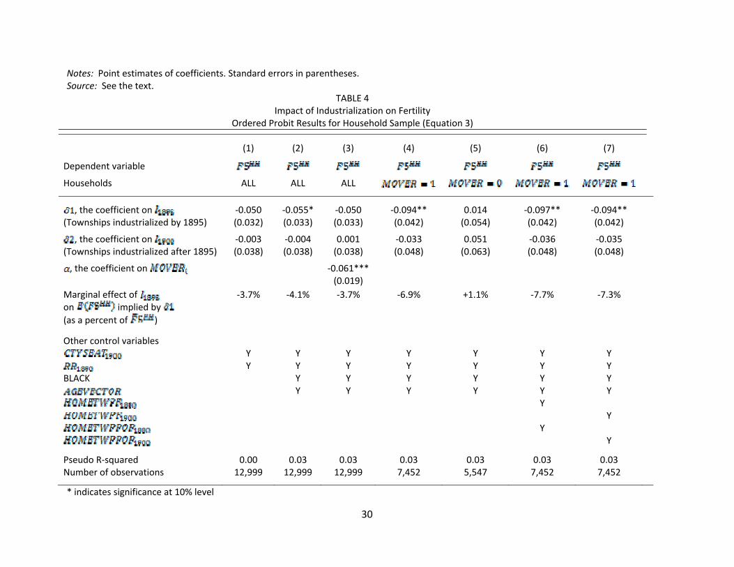
An  ordered  probit  estimator  is  used  for  Equation  3  because  values  for    are  discrete.28 

Coefficients and standard errors for  ,  , and   are reported in Table 4, but the coefficients no longer 

have a marginal effect  interpretation. The marginal effect  implied by    is  listed  lower  in the table.   In 

column  1  of  Table  4,  the  estimate  of  the  impact  of  industrialization  on  fertility  controlling  only  for 

variables available in the township sample indicates a negative correlation between   and pre‐1896 

industrialization of about 4.1 percent in the household sample compared to 7.4 percent in the township 

data weighted by population.   After adding race and age covariates in column 2, the implied reduction 

in fertility corresponding to pre‐1896 industrialization is 4.1 percent. 29 

,  the  indicator  for migration,  is  included  in  column  3  and  the  negative  coefficient 

implies that migrants had  lower  fertility.   Comparisons of coefficients  for the the sample of movers  in 

column 4 and non‐movers in column 5 shows that migrants who resided in townships industrialized by 

1895 had 6.9 percent lower fertility than migrants to non‐industrial townships.  On the other hand, non‐

movers  in  those  same  townships exhibited 1.1 percent higher  fertility, although  the coefficient  is not 

statistically significant.   This  is a striking result as  it  indicates that households who remained  in textile 

locations between  census  enumerations  exhibited no  change  in  fertility  relative  to  those households 

who remained in a non‐textile location. The industrialization process was correlated with lower fertility, 

as  earlier  results  have  indicated,  but  migrating  households  were  responsible  for  the  negative 

correlation. 

                                                       28 Poisson estimation does not remarkably alter the results. 

29 The analysis excludes households with a female spouse less than 15 years of age and greater than 50 years of age as these 

entries are more likely data errors than actual spousal matches. 

16  

There are at least three potential explanations for this result. First it is possible that migrants to 

textile townships were disproportionately from low‐fertility native townships and brought these fertility 

patterns  with  them.  But  adding  covariates  for  average  fertility  of  the  migrant's  home  township 

( )  and  population  of  the migrant's  home  township  ( ),  either  in  1880 

(Table 4 ‐ column 6) or 1900 (column 7), does not reduce the estimated impact of industrialization.30  

A second potential explanation is that movers to textile locations had lower initial fertility rates 

than  their native  township peers. Perhaps  these  low‐fertility households were  attracted  to  the  labor 

markets in industrial locales and brought their low fertility with them. If so, we would expect migrants to 

townships where mills were built  late  in  the 1881‐1900  timeframe  to exhibit  low  fertility as well, but 

that  is not the case. In every specification of Table 4 involving mover households (columns 4, 6, and 7) 

the  impact of being  in  an  industrial  township  in 1895  ( )  is  large  and negative while  the  impact of 

location  in  an  industrial  township  where  a  new mill  was  added  by  1900  ( )  is  less  negative  and 

statistically  insignificant. Migrants  exhibited  lower  fertility  than non‐migrants  in  textile  locations, but 

only  in  locations where  they had been exposed  to a  textile mill  for  five  years or  longer. Migrants  to 

townships where mills were built between 1896 and 1900 did not have  lower fertility rates than their 

peers.  This  points  not  to  selective migration  of  households,  but  to  a  different  fertility  response  to 

residence in a textile locale. 

This  gives  rise  to  a  third  explanation.  I document  below  that women  in  the households  that 

migrated to textile townships disproportionately chose textile occupations and experienced higher rates 

of  child  mortality.  In  addition,  the  loss  of  proximity  to  extended  family  for  migrants  might  have 

                                                       30 The variables   and   represent the   marital fertility of a household's home township 

measured in 1880 and 1900, respectively. The variables   and   represent the town 

population of a household's home township measured in 1880 and 1900, respectively. 

17  

contributed to higher costs of raising children.31 

MIGRATION, OCCUPATIONAL CHOICE, AND CHILD MORTALITY  

Occupational choice may have contributed to the differing impact of industrialization on movers 

and stayers. Since Ancestry.com did not report occupations for the sample used in Table 4,  I transcribed 

the occupation of the male and female household heads for the 2,342 households residing in townships 

in 1900  that were  industrialized between 1881 and 1900  from  the original census enumerations. The 

occupation shares in Table 5 show that 11 percent of male heads of migrant households were employed 

in  textile  jobs, compared with only 4 percent of stayers; 7 percent of migrant women compared  to 3 

percent  of  stayers were  in  textile  jobs.   Movers  also  had  a  higher  rate  of  employment  in  non‐farm 

occupations in general. 

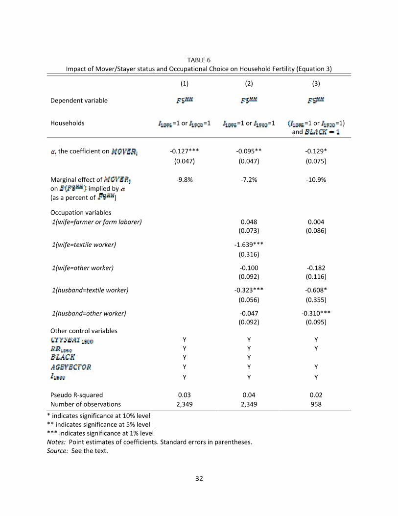
Both nonagricultural employment  categories were negatively  correlated with  fertility. When  I 

estimate fertility for households with occupations listed in the industrial townships as a function only of 

migration  in  column  1  of  Table  6,  fertility  is  strongly  negatively  correlated  with  migrant  status  in 

industrial  locales. After controlling for the occupations of the male and female household heads  in the 

sample in column 2, households with males and females in the textile industry have lower fertility, while 

the  relationship  between  fertility  and migration  is  reduced  by  approximately  25  percent  from  ‐9.8 

percent to ‐7.2 percent but remains significant. 

The impact of occupations was strong not only for white residents who were likely to experience 

textile employment, but also for black migrants who very rarely were textile workers.  Column 3 of Table 

6  limits  the  sample  to black households and  the  results are  largely unchanged. The  impact of  textile 

                                                       31 It does not appear that migrants' fertility rates were mismeasured due to leaving children behind, the so‐called “missing 

children” hypothesis. See Moehling, “Broken Homes”. Comparing the ratio of children present in the household to surviving 

children for young migrant mothers and young stayers in industrial townships, there is minimal difference.   The number of 

additional “missing” children for migrants relative to stayers is 3 out of 1,000, much smaller than the fertility differential 

observed in Table 4. 

18  

mills, it appears, extended beyond their own employees, perhaps because they altered the labor market 

for townships in general.  

Occupational  choice,  then,  can explain part of  the difference  in  fertility between movers and 

stayers in textile locations, but a significant portion of the correlation remains unexplained. One further 

hypothesis is that migration influenced infant mortality which, in turn, affected fertility. Higher rates of 

infant and child mortality  in  industrial  locations for migrating households  in 1900 may be the cause of 

lower observed fertility in 1900 if replacement is not perfectly achieved.32 

The 1900 Census asked married women how many children they had borne and how many were 

surviving.33 Using  the household  sample,  it  is  straightforward  to  calculate  a  child  survival  rate  as  the 

ratio of the number of children surviving to the number ever born, and then to examine the relationship 

between that number, industrial residence and migration.34 

I  estimate  the  relationship  between  a married  female's  reported  child  survival  rate  and  the 

presence of a textile mill in the household's 1900 township location, conditional on other characteristics 

of the household. The estimating equation is: 

    (4) 

 

where   is the observed child survival rate for household i in township j in 1900. Unlike  , the survival 

measure is not limited to the five years prior to the 1900 Census enumeration. Instead, the measure will 

reflect cumulative infant and child mortality over the entirety of a female's childbearing years and   

                                                       32 On the other hand, higher rates of infant mortality may lead to higher fertility by reducing birth intervals. 

33 Unfortunately, standardized infant and child mortality statistics for South Carolina townships in 1900 do not exist. 

34 A caveat is in order: this statistic will reflect the cumulative number of deaths of the household's children (in infancy or 

otherwise) over the entire span of the female's childbearing. It is impossible to determine from this data whether these deaths 

occurred in years before or after the introduction of a township's textile mills. 

19  

and   are no  longer relevant.  Instead  I construct a variable,  ,  that represents  the proportion of 

household  i's marital  duration  for which  township  j  housed  a  textile mill.  The  same  set  of  control 

variables are used to estimate Equation 4 as for Equation 3, and the same sample restrictions apply. 

Table 2 gives the mean and standard deviation of   and  . The results in column 1 of Table 7  

indicate no discernible difference in infant and child mortality rates between residents of industrialized 

and non‐industrialized townships.35 These are small numbers; the   coefficient in column 1 represents a 

reduction in survival rates of 0.9 percent. 

Adding migration status to the regression (Table 7 – column 2) does not affect the results. But in 

column 3,  I add an  interaction between mover status and  the  textile exposure measure,  , and  the 

estimates indicate that survival rates were significantly lower among movers to industrial locations than 

among their peers. A mover to a township with a textile mill present for the entirety of their marriage 

duration  experienced  a  reduction  in  child  survival  rates  of  3.7  percent  (0.031/0.84)  relative  to  non‐

movers or movers to non‐industrial  locales. The coefficients when occupations dummies are added to 

the  specification  in  column  4  indicate  that  the  occupational  choice  of migrants  largely  explains  the 

adverse child survival rates.   Female employment  in a textile mill had a  large negative correlation with 

child survival rates, while employment of the male had a more muted correlation. When the occupation 

dummies  are  added  the  coefficient  of  the  interaction  between mover  and  location  in  an  industrial 

household turns positive and is statistically insignificant.  For black residents (column 5), migration was 

similarly inconsequential for determining infant and child mortality after controlling for occupation. 

The  results  in Tables 6 and 7  indicate  that occupational choice may explain part of  the  lower 

observed  fertility  rates  among migrants  in  industrial  locales.  A  lower  child  survival  rate  in migrant 

households  is entirely attributable to occupational choice,  lending futher support to this conclusion.  If 

                                                       35 Restricting the sample to younger women or newly married couples does not change the result, and replacing   with the 

industrialization proxies employed previously generates the same conclusion.  

20  

differential  fertility among movers  to  industrial  locations was driven by  reductions  in survival  rates,  it 

appears  to have been  the  result of occupational choice. But a  significant portion of  the mover‐stayer 

fertility differential remains unexplained, even after controlling for occupation in Table 6.  

EVALUATING POTENTIAL MECHANISMS 

The introduction to his paper listed several ways in which economic growth may have affected 

fertility rates, and I evaluate those potential mechanisms in turn.   

First, the available evidence indicates that increases in the costs of raising children contributed 

to reduced fertility in textile locations.  Female occupation is a strong predictor of household fertility in 

the  sample  (Table  6),  and  low migrant  fertility  can  be  explained  in  part  by  higher  rates  of  female 

employment  in  textile  and  service  industries.  Fertility  is  most  strongly  associated  with  textile 

employment where employment would have prevented active  childrearing.   But  there  is a  significant 

impact among service workers as well. The arrival of textile mills increased demand for female‐provided 

services such as cooking, laundering, growing small amounts of crop and livestock, and boarding. These 

occupations  were  dominated  by  African  American  females  and  this  indirect  effect  can  explain  the 

reduction in fertility among this population. 

In addition, the observed difference in fertility for migrants relative to natives is consistent with 

a  different  cost  of  children  explanation:  the  costs  of  child  care.  For  natives  in  industrialized  locales, 

extended  family  could have  served  as  a backstop  for  childcare. But  for migrants  this option was not 

available.  Childcare  in  the mills  was  sporadically  supplied,  and most  families  would  have  relied  on 

household members for this service. The  lack of extended family members to perform this task would 

have resulted in an increase in the cost of raising children for migrants relative to natives and may have 

been another cause of the observed fertility differential.36 

                                                       36 This hypothesis is further supported by the fact that all migrants, in industrial locales and otherwise, exhibited lower fertility 

rates than their peers, and the absence of an extended family would have affected migrants no matter their final destination. 

21  

The  available  data  also  suggests  an  increase  in  population  density  as  an  important  factor  in 

inducing  lower  fertility.  In  the  township  results  of  Table  3,  controlling  for  the  town  population  of  a 

township reduces the coefficient on the industrialization proxy in column 5 by 29 percent for townships 

industrialized after 1895 and by 18 percent for those industrialized before that date.  

On the other hand, there is little evidence that child human capital or quality/quantity tradeoff 

concerns  drove  fertility  reduction.    Textile  mills  relied  on  low‐skilled  operatives,  and  there  is  no 

indication  that  textile manufacturing  increased  the  return  to human capital or  incentivized parents  to 

invest in child quality over quantity.37 A variant of the original quality/quantity hypothesis focuses on the 

potential impact of an increase in income on parental preference for quality over quantity. But this also 

has little support in the data as indicators for male occupational status (a proxy for household income) 

have a muted correlation with fertility  in comparison to those for female occupational status (a proxy 

for both household income and the opportunity cost of female time). (See Table 6.) 

Finally,  a decrease  in  the  labor opportunities of  children  is  an  improbable mechanism  in  this 

context. Available sources indicate that children represented a large proportion of workers in Southern 

mills, even when mills self‐reported their employment numbers.  Further, child labor legislation was not 

passed in South Carolina until 1903, well after the period examined in this paper. If changes in the labor 

opportunities of children drove the industrialization results, it must be that mill employment, extensive 

as it was, was less well renumerated than their previous employment, generally as farm laborers. This is 

a questionable assumption, in part because children, with their smaller and more dextrous hands, were 

                                                                                                                                                                               But migrants to textile locations exhibited even lower fertility rates and may also have been differentially affected by the loss of 

extended family. Their increased likelihood of being engaged in occupations which were incompatible with child‐rearing (for 

example, non‐agricultural occupations outside of their own home) would have increased their reliance on child care relative to 

migrants to other locations.  

37 See Becker, Hornung, Woessman, “Education”, for evidence that the textile industry in Prussia exhibited low returns to 

education relative to metal, rubber, and other industries. 

22  

actually better suited for some mill tasks than were adults. 

I conclude  that  increases  in child mortality,  the opportunity cost of  female  time, and  in other 

costs of raising children, including those resulting from increased population density, are the most likely 

explanations for lower fertility in South Carolina textile locations. 

 CONCLUSION 

Fertility decline  in  the 19th century United States has often been attributed  to an quickening 

pace of industrial activity. I exploit the fact that South Carolina's industrial experience between 1881 and 

1900 can be proxied by the textile industry in particular and evaluate the impact of the establishment of 

a textile mill on rural, marital fertility rates in South Carolina. Using a difference‐in‐difference approach, I 

estimate a 6 to 10% reduction in fertility following textile mill establishment. 

In  order  to  evaluate  potential mechanisms  to  explain  this  result,  I  build  a  household  data 

sample. I use the  location of male heads of household at two points  in time to measure migration and 

show that migrants exhibited substantially lower fertility than natives in industrial townships. Observing 

that migrating households were also more likely to be employed in the textile industry, I argue that an 

increase  in the costs of raising children,  including a heightened opportunity cost of female time,  led to 

lower household  fertility  in mill  locations.  I hypothesize  that  the  separation of migrating households 

from their extended families may also have raised the costs of childrearing and resulted in lower migrant 

fertility  in  industrial  locales.  Finally,  the  results  indicate  that  reductions  in  child  survival  rates  among 

migrating  industrial  workers  and  increases  in  population  density  also  contributed  to  the  observed 

fertility reduction. 

 REFERENCES

Atack, Jeremy, et al. “Did Railroads Induce or Follow Economic Growth? Urbanization and Population 

  Growth in the American Midwest 1850‐1860.” Social Science History 34, no. 2 (2010): 171‐197. 

23  

Beakley, Hoyt, and Jeffrey Lin. “Portage: Path Dependence and Increasing Returns in U.S. History.” 

  Unpublished Manuscript. 2010. 

Becker, Sascha O., Erik Hornung, and Ludger Woessmann. “Education and Catch‐up in the Industrial 

  Revolution.” American Economic Journal: Macroeconomics, Forthcoming. 

Brown, John C., and Timothy W. Guinnane. “Fertility Transition in a Rural, Catholic Population: Bavaria 

  1880‐1910.” Population Studies 56, no. 1 (2002): 35‐49. 

Carlton, David L. Mill and Town in South Carolina: 1880‐1920. Baton Rouge: Louisiana State University 

  Press, 1982. 

Carter, Susan B., Roger L. Ransom, and Richard Sutch. “Family Matters: The Life‐Cycle Transition and the 

Unparallelled Antebellum American Fertility Decline.” In History Matters: Essays on Economic 

Growth, Technology, and Demographic Change, edited by Timothy W. Guinnane, William A. 

Sundstrom and Warren Whatley, 271‐327. Stanford: Stanford University Press, 2002. 

Crafts, N.F.R. “Duration of Marriage, Fertility, and Women's Employment Opportunities in England and 

Wales in 1911.” Population Studies 43, no. 2 (1989): 325‐35. 

David, Paul, and William Sundstrom. “Old‐age Security Motives, Labor Markets and Farm Family Fertility 

in Antebellum America.” Explorations in Economic History 25, no.2 (1988): 164‐97. 

Davison Publishing Company. Davison's Textile Blue Book. Ridgewood, NJ, Multiple Years. 

Doepke, Matthias. “Accounting for Fertility Decline During the Transition to Growth.” Journal of 

Economic Growth 9, no. 3 (2004): 347‐383. 

______. “Child Mortality and Fertility Decline: Does the Barro‐Becker Model Fit the Facts?” Journal of 

Population Economics 18, no. 2 (2005): 337‐66. 

Easterlin, Richard A. “Does Human Fertility Adjust to the Environment?” The American Economic Review 

61, no. 2 (1971): 399‐407. 

24  

______. “Factors in the Decline of Farm Family Fertility in the United States: Some Preliminary Research 

Results.” Journal of American History 63, no.3 (1976): 600‐14. 

Galor, Oded, and David N. Weil. “The Gender Gap, Fertility, and Growth.” American Economic 

Review 86, no. 3 (1996): 375‐87. 

______. “Population, Technology, and Growth: From Malthusian Stagnation to the Demographic 

Transition and Beyond.” American Economic Review 90, no. 4 (2000): 806‐28. 

Guest, Avery M. “Social Structure and U.S. Inter‐State Fertility Differentials in 1900.” Demography 

18, no. 4 (1981): 465‐486. 

Guinnane, Timothy W.  “The Historical Fertility Transition and Theories of Long‐Run Growth: A Guide for 

Economists.” Journal of Economic Literature, Forthcoming. 

Haines, Michael R. “Economic History and Historical Demography: Past, Present and Future.” In The 

Future of Economics, edited by Alexander J. Field, 185‐253. Hingham, MA: Kluwer Academic 

Publishers, 1995. 

______. “The White Population of the United States, 1790‐1920.” In A Population History of 

North America, edited by Michael Haines and Richard Steckel, 305‐69. Cambridge: Cambridge 

University Press, 2000. 

Hazan, Moshe, and Binyamin Berdugo. “Child Labor, Fertility, and Economic Growth.” The Economic 

Journal 112, no. 482 (2002): 810‐28. 

Kalelmi‐Ozcan, Sebnem. “A Stochastic Model of Mortality, Fertility, and Human Capital Investment.” 

  Journal of Development Economics 70, no. 1 (2003): 103‐18. 

Kögel, Tomas, and Alexia Prskawetz. “Agricultural Productivity Growth and the Escape from the 

Malthusian Trap.” Journal of Economic Growth 6, no. 4 (2001): 337‐57. 

Lagerlö, Nils‐Petter. “Gender Equality and Long‐Run Growth.” Journal of Economic Growth 8, no. 4 

(2002): 403‐26. 

25  

Moehling, Carolyn M. “State Child Labor Laws and the Decline of Child Labor.” Explorations in Economic 

History 36, no. 1 (1999): 72‐106. 

______. “Broken Homes: The `Missing' Children of the 1910 Census.” Journal of Interdisciplinary History 

33, no. 2 (2002): 205‐33. 

North Atlantic Population Project and Minnesota Population Center. NAPP: Complete Count Microdata. 

NAPP Version 2.0 [computer files]. Minneapolis, MN: Minnesota Population Center [distributor], 

2008. 

Preston, Sameul H., Suet Lim, and S. Philip Morgan. “African‐American Marriage in 1910: Beneath the 

Surface of Census Data.” Demography 29, no. 1 (1992): 115. 

Ruggles, Steven, et al. Integrated Public Use Microdata Series: Version 4.0 (Machine‐Readable 

Database). Minneapolis, MN: Minnesota Population Center. 2008. 

Sah, Raaj K. “The Effects of Child Mortality Changes on Fertility Choice and Parental Welfare.” Journal of 

Political Economy 99, no. 3 (1991): 582‐606. 

Sanderson, Warren. “Quantitative Aspects of Marriage, Fertility, and Family Limitation in Nineteenth 

Century America: Another Application of the Coale Specifications.” Demography 16, no. 3 

(1979), 339‐58. 

Schapiro, Morton O. “Land Availability and Fertility in the United States, 1760‐1870.” This JOURNAL 42, 

no. 3 (1982): 577‐600. 

Schultz, T. Paul. “Changing World Prices, Women's Wages, and the Fertility Transition: Sweden, 1860‐ 

1910.” Journal of Political Economy 93, no. 6 (1985): 1126‐49. 

Steckel, Richard H. “The Fertility Transition in the United States: Tests of Alternative Hypotheses.” In 

Strategic Factors in Nineteenth Century American Economic History, Edited by Claudia Goldin 

and Hugh Rockoff, 351‐74. Chicago: University of Chicago Press, 1992. 

Stover, John R. The Railroads of the South, 1865‐1900. Chapel Hill: North Carolina University Press, 1955. 

26  

Tamura, Robert. “Human Capital and the Switch from Agriculture to Industry.” Journal of Economic 

Dynamics and Control 27, no. 2 (2002): 207‐42. 

Tang, Anthony M. Economic Development in the Southern Piedmont, 1860‐1950: Its Impact on 

Agriculture. Chapel Hill, NC: University of North Carolina Press, 1958. 

Thompson, Holland. From the Cotton Field to the Cotton Mill: A Study of the Industrial Transition in 

North Carolina. New York: The MacMillan Company, 1906. 

Todd, Petra E. “Matching Estimators.” In The New Palgrave Dictionary of Economics, edited by Steven N. 

Durlauf and Lawrence E. Blume. New York: Palgrave Macmillan, 2008. 

United States Bureau of Labor. Report on Condition of Woman and Child Wage‐Earners in the United 

States. Washington, DC.: Government Printing Office, 1910. 

United States Commissioner of Labor. Cost of Production: The Textiles and Glass. Washington, DC:  

Government Printing Office, 1892. 

United States of America, Bureau of the Census. Tenth Census of the United States, 1880.Washington, 

DC: Government Printing Office, 1880. 

United States of America, Bureau of the Census. Index to the 1900 United States Federal Census. Digital 

copy of original records in the National Archives, Washington DC. Available at 

http://www.ancestry.com, subscription database, 2008. 

Vinovskis, Maris. “Socio‐economic Determinants of Interstate Fertility Differentials in the United States 

in 1850 and 1860.” Journal of Interdisciplinary History 6, no. 3 (1976): 375‐96.  

Wahl, Jenny Bourne. “Trading Quantity for Quality: Explaining the Decline in American Fertility in the 

Nineteenth Century.” In Strategic Factors in Nineteenth Century American Economic History, 

edited by Claudia Goldin and Hugh Rockoff, 375‐97. Chicago: University of Chicago Press, 1992. 

Wright, Gavin. Cheap Labor and Southern Textiles before 1880. This JOURNAL 39, no, 3 (1979): 655‐80. 

27  

Yasuba, Yasukichi. Birth Rates of the White Population in the United States, 1800‐1860: An Economic 

Study. Baltimore: Johns Hopkins University Press, 1962. 

 

 

 

 

 

 

TABLES TABLE 1 

Township Data Variable Summary              

 All 

Townships  

StandardDeviation

 

No TextileMill 

By 1900 

First Mill Built  1881‐

1890 

First Mill Built  1891‐

1895 

First Mill Built  

1896‐1900

   1.42  0.14 1.43 1.39 1.36  1.40

   0.05  0.22 0.03 0.13 0.36  0.27

   0.03  0.11 0.02 0.07 0.10  0.16

  0.68  0.05 0.68 0.64 0.63  0.65

   1.08  0.09 1.07 1.08 1.08  1.11

 

0.57  0.20 0.58 0.44 0.47  0.50

   1.22  0.18 1.24 1.08 1.10  1.12

   0.06  0.24 0.03 0.13 0.43  0.27

   0.07  0.12 0.05 0.18 0.18  0.26

  0.65  0.05 0.65 0.65 0.61  0.62

   1.03  0.13 1.03 1.00 1.04  1.05

  

0.58  0.20 0.60 0.39 0.45  0.46

N   341    301 8 14  11

Notes:  Sample includes all Non‐Coastal Townships, with no textile mill by 1880 and 1900 Town Population . Corresponds to results in Tables 3 and 9. Source:  See the text.

TABLE 2 

1900 Variable Summary for Household Data      

     

28  

    Sample Mean 

Standard Deviation 

 = Number own children   in 1900 household i  1.22  1.00    0.11  0.31    0.07  0.26 

   0.10  0.29 

  0.49  0.50 

  30.49  5.7 

  26.94  6.1    0.57  0.49 

 = Survival rate of children ever born  0.84  0.25 

 = Percent of marriage duration for which textile mill is present   0.11  0.30      

a) Conditional on remaining in South Carolina Notes:  Corresponds to results in Tables 4, 6, and 7 Source:  See the text. 

29  

TABLE 3 Impact of Industrialization on Fertility 

Difference‐in‐Difference Estimation Results for Township Sample (Equation 2)        

    

     

Full Sample  Trimmed Sample ‐ Baseline  Robustness Checks (1)  (2)  (3)  (4)  (5)  (6)    (8) 

Dependent variable                 

Townships   ALL  ALL  Eliminate Coastal and Town Pop. 

 Counties 

See (3)  See (3)  See (3) Weighted by 

 

See (3)  See (3) 

, the coefficient on    ‐0.093***  ‐0.075**  ‐0.084**  ‐0.074*  ‐0.052  ‐0.088***  ‐0.074**  ‐0.097** (Townships industrialized by 1895)  (0.035)  (0.037)  (0.041)  (0.042)  (0.042)  (0.029)  (0.033)  (0.044) 

, the coefficient on    ‐0.0867**  ‐0.074*  ‐0.074  ‐0.058  ‐0.052  ‐0.084*  ‐0.047*  ‐0.079 (Townships industrialized after 1895)   (0.041)  (0.042)  (0.045)  (0.046)  (0.045)  (0.037)  (0.043)  (0.048) 

Percent reduction in fertility   7.8%  6.3%  6.9%  6.0%  4.3%  7.4%  10.0%  7.3% implied by                           

Other control variables                  

    Y             

    Y             

   Y  Y  Y  Y  Y  Y  Y  Y 

         Y  Y       

         Y  Y       

           Y       

           Y                        

F‐statistic   3.82  3.32  2.25  2.35  4.12  851.21  2.48  2.40 Number of observations  391  391  341  341  341  341  341  341                   

* indicates significance at 10% level ** indicates significance at 5% level *** indicates significance at 1% level (a) In Column (7)   becomes   and   represents only those mills built between 1898 and 1900. 

30  

Notes:  Point estimates of coefficients. Standard errors in parentheses. Source:  See the text. 

TABLE 4 Impact of Industrialization on Fertility 

Ordered Probit Results for Household Sample (Equation 3)  

       

(1)  (2)  (3)  (4)  (5)  (6)  (7)   

Dependent variable                 

Households  ALL  ALL  ALL           

, the coefficient on    ‐0.050  ‐0.055*  ‐0.050  ‐0.094**  0.014  ‐0.097**  ‐0.094**   (Townships industrialized by 1895)  (0.032)  (0.033)  (0.033)  (0.042)  (0.054)  (0.042)  (0.042)   

, the coefficient on    ‐0.003  ‐0.004  0.001  ‐0.033  0.051  ‐0.036  ‐0.035   (Townships industrialized after 1895)   (0.038)  (0.038)  (0.038)  (0.048)  (0.063)  (0.048)  (0.048)   

, the coefficient on        ‐0.061***                 (0.019)           

Marginal effect of     ‐3.7%  ‐4.1%  ‐3.7%  ‐6.9%  +1.1%  ‐7.7%  ‐7.3%   on   implied by                   

(as a percent of  )                                  

Other control variables                    Y  Y  Y  Y  Y  Y  Y   

   Y  Y  Y  Y  Y  Y  Y   BLACK     Y  Y  Y  Y  Y  Y   

     Y  Y  Y  Y  Y  Y                Y                    Y   

             Y                    Y   

                 

Pseudo R‐squared   0.00  0.03  0.03  0.03  0.03  0.03  0.03   Number of observations   12,999  12,999  12,999  7,452  5,547  7,452  7,452                    

* indicates significance at 10% level 

31  

** indicates significance at 5% level *** indicates significance at 1% level Notes:  Point estimates of coefficients. Standard errors in parentheses. Source:  See the text.    

TABLE 5 Male and Female Occupation, Tabulated by Mover/Stayer status

        

     Male 

 

   

 Female 

 

   Farmers and Farm Laborers 

Textile Workers 

 Other 

 Unemployed 

 Farmers and Farm Laborers 

Textile Workers 

 Other 

 Unemployed 

Proportion of all stayers   0.73  0.04  0.22  0.01    0.14  0.01  0.08  0.77 Proportion of all employed stayers   0.74  0.04  0.22  ‐‐‐    0.62  0.03  0.35  ‐‐‐                    

Proportion of all movers   0.60  0.11  0.29  0.01    0.12  0.02  0.07  0.79 Proportion of all employed movers   0.60  0.11  0.29  ‐‐‐    0.58  0.07  0.35  ‐‐‐                    

                   

Total   0.65  0.08  0.26  0.01    0.13  0.01  0.07  0.79                    

Source and notes:  See the text.  The Other category is comprised mostly of service occupations. 

 

32  

 TABLE 6 

Impact of Mover/Stayer status and Occupational Choice on Household Fertility (Equation 3)        

   (1)  (2)  (3)         

Dependent variable               Households  =1 or  =1  =1 or  =1  =1 or  =1) 

and          , the coefficient on    ‐0.127***  ‐0.095**  ‐0.129* 

  (0.047)  (0.047)  (0.075) 

       Marginal effect of     ‐9.8%  ‐7.2%  ‐10.9% on   implied by         

(as a percent of  )       

Occupation variables        

 1(wife=farmer or farm laborer)      0.048  0.004      (0.073)  (0.086)        

 1(wife=textile worker)      ‐1.639***   

     (0.316)          

 1(wife=other worker)      ‐0.100  ‐0.182      (0.092)  (0.116)        

 1(husband=textile worker)      ‐0.323***  ‐0.608* 

     (0.056)  (0.355)        

 1(husband=other worker)      ‐0.047  ‐0.310***      (0.092)  (0.095) Other control variables        

   Y  Y  Y    Y  Y  Y 

  Y  Y   

   Y  Y  Y 

   Y  Y  Y        

Pseudo R‐squared   0.03  0.04  0.02 

Number of observations   2,349  2,349  958 

* indicates significance at 10% level ** indicates significance at 5% level *** indicates significance at 1% level Notes:  Point estimates of coefficients. Standard errors in parentheses. Source:  See the text. 

33  

TABLE 7 Regression Results for Child Survival Rates in the Household Sample (Equation 4) 

           

   (1)  (2)  (3)  (4)  (5)              

Dependent variable               

Households   ALL  ALL  ALL  =1 or  =1 

( =1 or =1) and 

            

 ‐ coefficient on     ‐0.0085  ‐0.0079  0.013  ‐0.011  ‐0.008 

  (0.0078)  (0.0078)  (0.013)  (0.023)  (0.041)             

, the coefficient on MOVER     ‐0.0049  ‐0.0010  ‐0.024  ‐0.001     (0.005)  (0.005)  (0.021)  (0.035)            

MOVER x           ‐0.031**  0.0045  0.000 

      (0.016)  (0.027)  (0.047)             

Percent change in    1.0%  0.9%  1.5%  0.8%  1.0% survival rate implied by                        

Occupation variables             1(wife=farmer or farm laborer)           ‐0.021  ‐0.006           (0.017)  (0.021)             1(wife=textile worker)            ‐0.140**              (0.058)               1(wife=other worker)            ‐0.015  ‐0.006            (0.021)  (0.021)             1(husband=textile worker)            ‐0.076***  ‐0.05            (0.018)  (0.09)             1(husband=other worker)            ‐0.037  ‐0.058**         (0.013)  (0.022) Other control variables               

   Y  Y  Y  Y  Y    Y  Y  Y  Y  Y 

  Y  Y  Y  Y   

   Y  Y  Y  Y  Y            

Adjusted R‐squared   0.02  0.02  0.02  0.03  0.02 Number of observations   11,188  11,188  11,188  2,284  890               

* indicates significance at 10% level ** indicates significance at 5% level *** indicates significance at 1% level Notes:  Point estimates of coefficients. Standard errors in parentheses. 

34  

Source:  See the text.        

FIGURES FIGURE 1 

South Carolina Mill Establishment: 1881‐1900 

 Source: Davison Publishing Company, Davison's Blue Book.

            

35  

FIGURE 2 Residual Fertility (1880‐1899) in Non‐Industrial Townships, by future industrial status

 

 Notes:  Plotted residuals from a regression of annual fertility rates from 1881 to 1899 in townships that do not contain a textile mill in that year on a township fixed effect and a constant. Mean residuals are plotted for two types of townships: those that do not industrialize in the 20‐year window (“Not industrialized by 1900”) and those that industrialize at some point before 1900 but have not done so by year t (“Industrialized, but not yet”).  See “Difference‐in‐Difference Results” for more details. Source:  See the text. 

FIGURE 3 F5 Fertility Rates for Industrialized and Non‐Industrialized South Carolina 

 Townships (Left Panel) and for all South Carolina, the South, U.S. (Right Panel)

Notes:   Left‐hand panel  includes only  townships  in  the baseline sample  (non‐coastal,  town population <2500) from Table 3, Column 3.   Right‐hand panel, All South Carolina  includes all S.C. townships while Paper Sample is the baseline sample from Table 3.  “All South” includes all former Confederate states.   Source:    Left‐hand  panel:  see  the  text.    Right‐hand  panel:  United  States  of  America,  Bureau  of  the Census, Tenth Census, Twelfth Census. 

36  

APPENDIX 1: THE OCCUPATION OF SOUTH CAROLINIANS IN 1900  

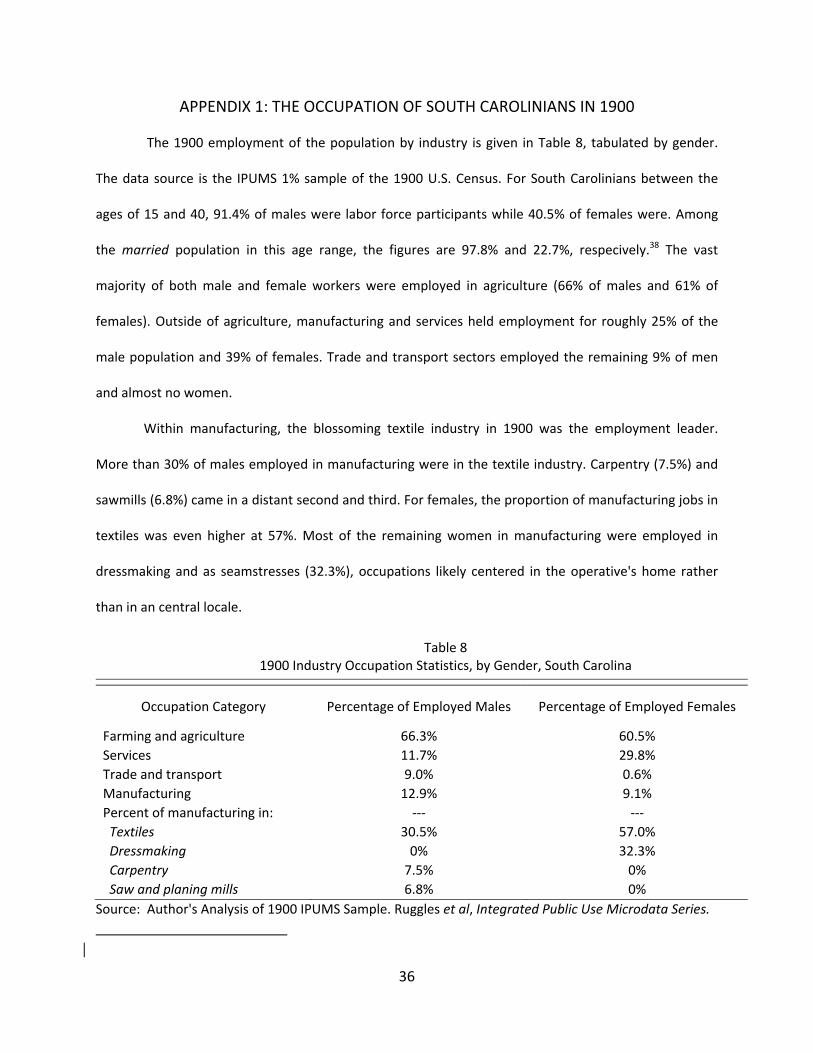
 The 1900 employment of the population by  industry  is given  in Table 8, tabulated by gender. 

The data source  is  the  IPUMS 1% sample of  the 1900 U.S. Census. For South Carolinians between  the 

ages of 15 and 40, 91.4% of males were  labor force participants while 40.5% of females were. Among 

the married  population  in  this  age  range,  the  figures  are  97.8%  and  22.7%,  respecively.38  The  vast 

majority of both male  and  female workers were  employed  in  agriculture  (66% of males  and  61% of 

females). Outside of agriculture, manufacturing and services held employment  for roughly 25% of  the 

male population and 39% of females. Trade and transport sectors employed the remaining 9% of men 

and almost no women.  

Within manufacturing,  the  blossoming  textile  industry  in  1900 was  the  employment  leader. 

More than 30% of males employed in manufacturing were in the textile industry. Carpentry (7.5%) and 

sawmills (6.8%) came in a distant second and third. For females, the proportion of manufacturing jobs in 

textiles was  even higher  at 57%. Most of  the  remaining women  in manufacturing were  employed  in 

dressmaking and as  seamstresses  (32.3%), occupations  likely centered  in  the operative's home  rather 

than in an central locale.

Table 8 1900 Industry Occupation Statistics, by Gender, South Carolina 

 

Occupation Category  Percentage of Employed Males  Percentage of Employed Females 

Farming and agriculture   66.3% 60.5%

Services   11.7% 29.8%

Trade and transport   9.0% 0.6% Manufacturing   12.9% 9.1% Percent of manufacturing in:   ‐‐‐ ‐‐‐   Textiles   30.5% 57.0%

  Dressmaking   0% 32.3%

  Carpentry   7.5% 0%   Saw and planing mills   6.8% 0% Source:  Author's Analysis of 1900 IPUMS Sample. Ruggles et al, Integrated Public Use Microdata Series. 

                                                        

37  

 It is clear from Table 8 that industrial employment (production at a centralized location) in South 

Carolina  in  this  time period was  limited almost exclusively  to  textile mills. All other employment was 

either agricultural or decentralized (dress‐making, carpentry, etc.). The sole exception is the small level 

of employment among men in the region's saw mills. But as only 0.8% of males were so‐employed, the 

contribution of saw milling to industrial employment will be ignored. 

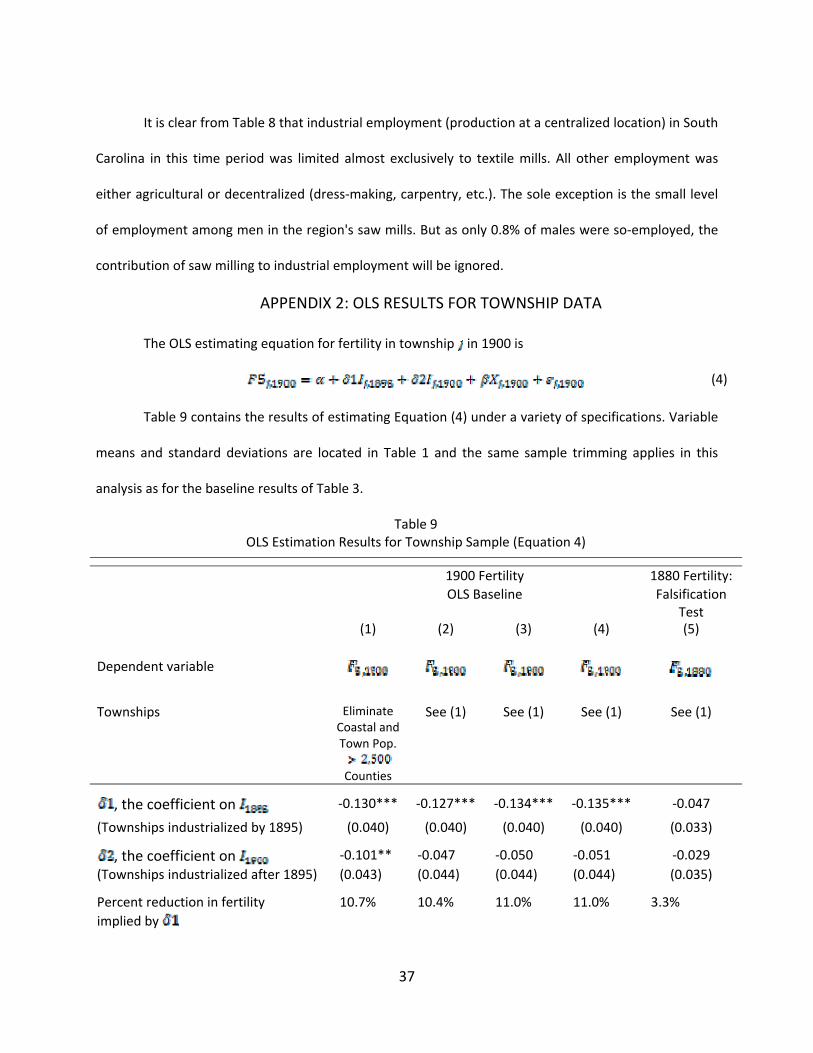
APPENDIX 2: OLS RESULTS FOR TOWNSHIP DATA 

The OLS estimating equation for fertility in township   in 1900 is  

    (4) 

Table 9 contains the results of estimating Equation (4) under a variety of specifications. Variable 

means and  standard deviations are  located  in Table 1 and  the  same  sample  trimming applies  in  this 

analysis as for the baseline results of Table 3. 

Table 9OLS Estimation Results for Township Sample (Equation 4) 

     

  1900 Fertility 1880 Fertility:

  OLS Baseline Falsification Test

  (1) (2) (3) (4)  (5)            

Dependent variable                       

Townships   Eliminate Coastal and Town Pop. 

 Counties 

See (1) See (1) See (1)  See (1)

            

, the coefficient on     ‐0.130*** ‐0.127*** ‐0.134*** ‐0.135***  ‐0.047

(Townships industrialized by 1895)   (0.040) (0.040) (0.040) (0.040)  (0.033)           

, the coefficient on      ‐0.101**   ‐0.047  ‐0.050   ‐0.051  ‐0.029

(Townships industrialized after 1895)    (0.043)   (0.044)   (0.044)   (0.044)  (0.035)           

Percent reduction in fertility    10.7%   10.4%   11.0%   11.0%    3.3% 

implied by                            

38  

Other control variables               Y Y Y Y  Y

     Y Y Y        Y Y Y   

       Y Y          Y Y   

         Y              Adjusted R‐squared  0.05 0.13 0.14 0.14  0.01Number of observations  341 341 341 341  341

* indicates significance at 10% level ** indicates significance at 5% level *** indicates significance at 1% level Notes:  Point estimates of coefficients. Standard errors in parentheses. Source:  See the text.  

Analogous  to  the structure of Table 3, Column  (1) of Table 9  includes only   as a 

component of  . Subsequent columns include additional controls for town population and the non‐

white population ratio in 1900 (Column (2)), and the marriage rate and sex ratio for age 18‐42 (Column 

(3)).  In  each  case,  the  impact  of  industrialization  on  fertility  as measured  by    remains  large  and 

significant. 

As discussed previously, railroad presence may have been a driver for textile mill location in the 

late 1890s and could also have affected fertility. Including a measure for railroad presence (Column (4)) 

does not significantly alter the estimated impact of industrialization and the impact of the railroad itself 

is neither economically nor statistically significant.39 

Table 1 indicates that fertility rates in townships that would eventually house textile mills were 

lower  in 1880, before mill establishment.  In Column  (5),  I undertake a  falsification  test  to determine 

whether this difference is significant. I estimate the impact of a textile mill built between 1881 and 1900 

on  fertility  in 1880. Control variables are the same as those  in Column  (1).40 The difference  in ex ante 

                                                        Including this variable in the estimation does not affect the conclusions in this section, was not recreated for 1880 and 1900, 

and thus is not included in the difference‐in‐difference specifications. 

 (all measured in 1900) as control variables generates similar conclusions. 

39  

fertility is not significantly different from zero, but the point estimate still indicates a 3.3% difference in 

fertility  in 1880. For this reason,  I utilize a difference‐in‐difference estimator  in the text and  in Table 3 

and a matching estimator in Appendix 3. 

APPENDIX 3: A PROPENSITY SCORE ESTIMATOR 

The difference‐in‐difference estimator employed in the text is one way of dealing with potential 

differences in ex ante characteristics of industrializing townships. A matching estimator is another. 

 

Table 10 Propensity Score Matching Estimates ‐ Township Sample

      

     

Model   LLM KM      

Dependent variable         

Townships   Baseline Sample Baseline Sample

  (From Table 3) (From Table 3)      

, the coefficient on     ‐0.135*** ‐0.137** (Townships industrialized by 1895)   (0.068) (0.049) 

, the coefficient on     ‐0.046 ‐0.039 (Townships industrialized after 1895)   (0.037) (0.032)      

Percent reduction in fertility   11.1% 11.2% implied by          

* indicates significance at 10% level ** indicates significance at 5% level *** indicates significance at 1% level Notes:  Point estimates of coefficients. Standard errors in parentheses. Source:  See the text. 

 

The  estimate  is  performed  in  two  steps.  First,  I  generate  a  propensity  score  for  textile mill 

establishment based on observables of a township  in 1880:  its population, county seat status, “town” 

population percentage, marriage rate among fertile females (age 18 to 42), sex ratio for ages 18 to 42 

and  the percentage of  the population  that  is non‐white.  I  run a probit  for   and   on  these 

40  

variables and generate, for each township, the predicted probability of receiving a textile mill  in these 

two time periods. 

Next,  I  use  a  local  linear matching  (LLM)  and  a  kernel matching  (KM)  estimator,  both with 

bootstrapped  standard  errors,  to  generate  an  estimated  effect  of  industrialization  on  the  treated 

townships.  For  each  township    that  industrializes  between  1881  and  1900,  the matching  estimator 

compares  the  value  of    to  the weighted  average  of    for  non‐industrializing  townships 

where the weights are inversely proportional to the difference between the propensity score for   and 

that for the other townships.41 A matching estimator, then, calculates the difference in fertility between 

locations with  similar probabilities of  industrializing, given 1880  characteristics. This process prevents 

estimates for the fertility impact that are driven by non‐industrial townships that are entirely dissimilar 

to  the  industrial  set.42 Results are  located  in Table 10. Both a  kernel match and a  local  linear match 

generate results consistent with those detailed in Table 3, although the point estimates are larger. 

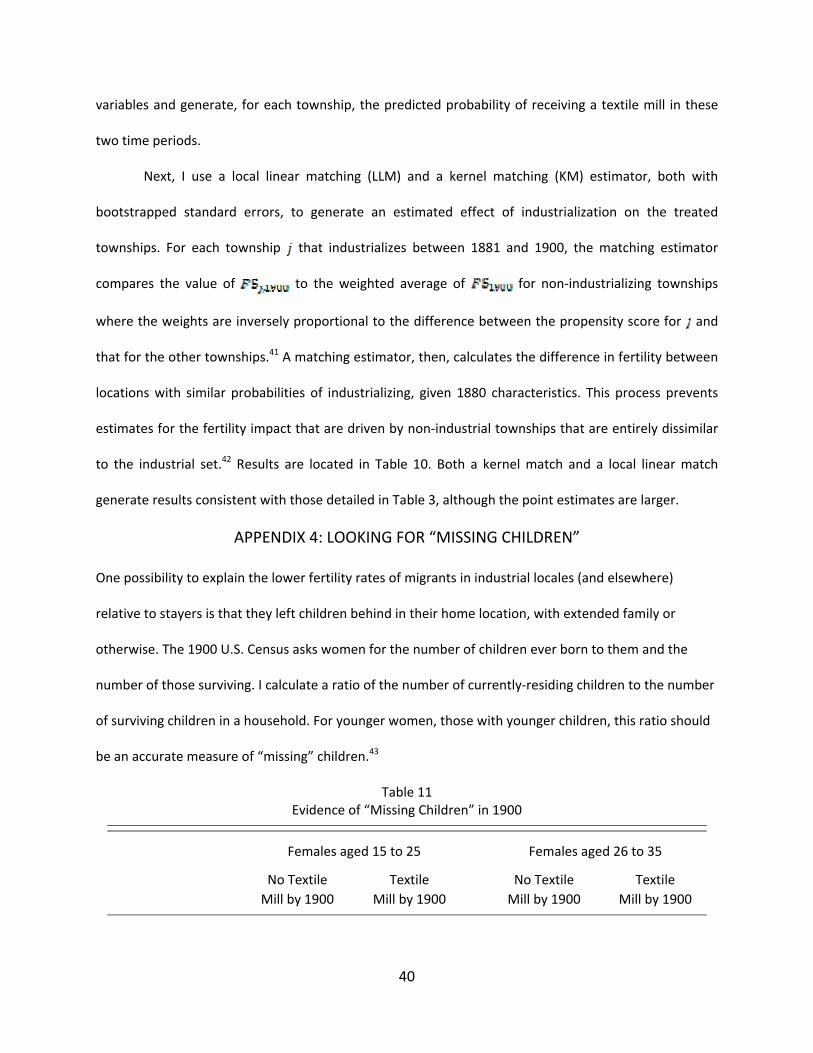
APPENDIX 4: LOOKING FOR “MISSING CHILDREN” 

One possibility to explain the lower fertility rates of migrants in industrial locales (and elsewhere) 

relative to stayers is that they left children behind in their home location, with extended family or 

otherwise. The 1900 U.S. Census asks women for the number of children ever born to them and the 

number of those surviving. I calculate a ratio of the number of currently‐residing children to the number 

of surviving children in a household. For younger women, those with younger children, this ratio should 

be an accurate measure of “missing” children.43 

Table 11Evidence of “Missing Children” in 1900 

 

   Females aged 15 to 25    Females aged 26 to 35 

  No Textile Textile   No Textile  Textile

  Mill by 1900 Mill by 1900   Mill by 1900  Mill by 1900           

            

41  

Township stayers   0.968  0.950   0.958 0.980

Township migrants  0.956  0.953   0.946 0.951

  N=4,283   N=4,728 

Notes:  Cells contain the average ratio of children present to surviving children reported. Source:  See the text.  

Table 11 displays the average ratio of children present to children surviving, by migrating status 

and township industrialization status, for two different age brackets. The first line of the table shows the 

average  percentage  of  surviving  children  present  in  the  household  of  township  “stayers”  in  1900, 

divided  between  townships  with  and  without  a  textile  mill.  The  second  line  shows  the  same  for 

migrants.  

From these results, I detect no notable increase in the number of “missing” children for migrants 

relative to natives in either non‐textile or textile locales. The first panel, females aged 15 to 25, can be 

reasonably assumed  to contain  females whose children are  too young  to have  left  the  family  to  seek 

separate  residence.  The  difference  between  the  ratio  for  township  migrants  in  mill  and  non‐mill 

townships  amounts  to  3  “missing”  children  out  of  1,000, much  smaller  than  the  fertility  difference 

observed  in Table 4. Panel  two,  females aged 26  to 35,  is more  likely  to  include  the effects of adult 

children striking out on their own and  is therefore  less preferable for answering the question at hand. 

Nonetheless, the second panel of results indicates a higher ratio of children present in the household in 

industrialized  townships  relatve  to  non‐mill  locales  and  there  does  not  seem  to  be  a  difference  by 

migration status. I conclude that the fertility difference between natives and migrants is not attributable 

to “missing” children.