industrial rotating kiln simulation - opus at uts: home heat transfer paths in the transverse...
TRANSCRIPT

Industrial Rotating Kiln Simulation
This thesis is presented for the degree of Doctor of Philosophy
Faculty of Science
University of Technology, Sydney
1999
Submitted by Dennis Van Puyvelde, B. Chem. Eng. (Hons)

Industrial Rotating Kiln Simulation – Page ii.
Certificate of Authorship/Originality
I certify that the work in this thesis has not been previously submitted for a degree
nor has it been submitted as part of requirements for a degree except as fully
acknowledged within the text.
I also certify that the thesis has been written by me. Any help that I have received in
my research work and the preparation of the thesis itself has been acknowledged. In
addition, I certify that all information sources and literature used are indicated in the
thesis.
Signature of Candidate
________________________________

Industrial Rotating Kiln Simulation – Page iii.
ABSTRACT
A new industrial process is being developed to allow the commercial recovery of oil
from oil shales. As part of this process, a rotating kiln is used to pyrolyse the organic
component of the oil shales. The configuration and application of this rotating kiln is
unique and hence previous rotating kiln models cannot be used to predict the solid
behaviour in the current processor. It is the aim of this work to develop
mathematical models which allow the prediction of mixing, segregation and heat
transfer in industrial rotating kilns, especially with respect to the new rotating kiln
technology trialed in the oil shale industry.
Experiments were developed to observe and measure the mixing and segregation
behaviour of solids in rotating drums. These experiments used image analysis and
provided quantitative results. Further experiments were carried out to allow suitable
scaling parameters to be developed.
All the mixing experiments followed a constant mixing rate until the bed became
fully mixed. The mixing rate and the final amount of mixing depended on the
rotational velocity, the drum loading, the particle size and the material ratio. The
segregation dynamics occurred too fast to be measured. However the final segregated
state was measured and depended on the rotational velocity and the differences in
particle sizes. Scaling parameters were developed that related the mixing and
segregation results to the operational variables of the rotating kiln.
Mathematical models were derived for the mixing and segregation of solids in a
rotating kiln and these models included the developed scaling parameters so that
these models would be useful for the prediction of the solid behaviour in industrial
rotating kilns. The mathematical models were applied to independent experiments
and it was found that they predicted the mixing and segregation to within the

Industrial Rotating Kiln Simulation – Page iv.
experimental error, even for different sized drums indicating that the developed
scaling parameters were suitable.
A computational simulation of the industrial rotating kiln processor was developed
by combining the mathematical models of the mixing and segregation with heat
transfer modelling applicable to this industrial rotating kiln. A case study was
completed to study the behaviour of the industrial rotating kiln by changing
operational variables, such as the rotational speed and the particle size.
The developed simulation can be used to predict the dynamic behaviour of the
rotating kiln used in the emerging oil from oil shale industry. This simulation can
assist in further commercialisation of this new industrial process.

Industrial Rotating Kiln Simulation – Page v.
ACKNOWLEDGEMENTS
I would like to thank the following for their assistance during the course of my PhD
research.
Firstly my academic and industrial supervisors: Dr. Brent Young from the University
of Calgary, Canada, Professor Michael Wilson from the University of Technology,
Sydney, Dr. Stephen Grocott and Mr. Jim Schmidt from Southern Pacific Petroleum
(Development). Dr. Young deserves a special mention by going beyond his initial
commitment as a local supervisor and maintaining excellent supervision after his
relocation to Canada.
Financial commitment for the project was provided by Southern Pacific Petroleum
N.L. and the University of Technology, Sydney. This financial assistance made the
work possible and allowed me to present my work at various conferences.
All the present and past members of the Chemical Technology and Engineering
Research Group – especially Dr. Adam Berkovich, for helpful discussions. Especially
the ones held at The Duke of Cornwell.
The Faculty of Science workshop and Mr. Alan Barnes were very helpful in the
design of the experimental equipment.
The Faculty of Science Research Degrees Committee and the University’s Chemical
Society for showing me there is more to a research degree than research.
My parents and family.
Lastly and most importantly, I would like to take the opportunity to thank my wife
and best friend Shannon Elizabeth for her wonderful support throughout the last
three years of my life.

Industrial Rotating Kiln Simulation – Page vi.
Table of content
Certificate of Authorship/Originality ii
ABSTRACT
ACKNOWLEDGEMENTS v
Table of content vi
Table of Figures xiii
CHAPTER 1 1
Introduction. 1
1.1 APPLICATIONS AND DESCRIPTIONS OF ROTARY KILNS 1
1.2 “OIL FROM OIL SHALE” PROCESS 2
1.2.1 Oil shale in Australia 2
1.2.2 The Stuart project 3
1.2.3 The AOSTRA-Taciuk Processor 4
1.3 RESEARCH OBJECTIVES 6
1.4 THESIS STRUCTURE 7
1.5 CHAPTER SUMMARY 7
i i

Industrial Rotating Kiln Simulation – Page vii.
CHAPTER 2 8
Mixing, segregation and heat transfer mechanisms of granular materials. 8
2.1 MIXING OF GRANULAR MATERIALS 8
2.1.1 Shear mixing of granular materials 10
2.1.2 Convective mixing of granular materials 10
2.1.3 Diffusive mixing of granular materials 11
2.2 SEGREGATION OF GRANULAR MATERIALS 12
2.2.1 Percolation segregation mechanism of granular materials 13
2.2.2 Flow or trajectory segregation mechanism of a granular material
14
2.2.3 Vibration segregation mechanism of a granular material 15
2.3 HEAT TRANSFER IN GRANULAR MATERIALS 15
2.3.1 Heat transfer paths between particles 15
2.3.2 Heat transfer in a granular medium 17
2.4 CHAPTER SUMMARY 18
CHAPTER 3 20
Rotating drums and kilns – literature review. 20
3.1 TRANSVERSE MOTION IN A ROTATING DRUM 21
3.1.1 Transverse bed regimes 21
3.1.2 The transverse rolling regime in a rotating drum 23
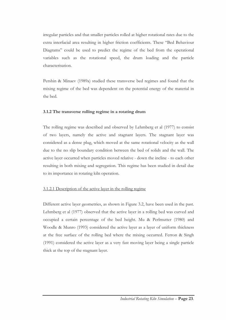
3.1.2.1 Description of the active layer in the rolling regime 23
3.1.2.2 Description of the stagnant layer in the rolling regime 26
3.1.2.3 Description of the mixing and segregation in the rolling
regime 27
3.2 AXIAL MOTION IN A ROTATING DRUM 33
3.2.1 Motion in the axial section of a rotating drum 33
3.2.2 Residence times in rotating kilns 34
3.2.3 Mixing and segregation in the axial direction 36
3.3 HEAT TRANSFER IN ROTARY KILNS 37

Industrial Rotating Kiln Simulation – Page viii.
3.3.1 Heat transfer paths in the transverse direction of a rotary kiln 38
3.3.2 Review of rotary kiln heat transfer modelling 39
3.4 SCALE UP THEORY. 40
3.5 CHAPTER SUMMARY 41
CHAPTER 4 43
Experimental design. 43
4.1 PARTICLE AND GRANULAR MEDIUM CHARACTERISATION 43
4.1.1 Physical properties of Stuart oil shale 44
4.1.1.1 Particle sizes 44
4.1.1.2 Static angle of repose 44
4.1.1.3 Bulk density 45
4.1.2 Chemical properties of Stuart oil shale 47
4.1.3 Preparation of the raw materials 48
4.2 ROTATING DRUM DESIGN 49
4.3 IMAGE CAPTURE AND ANALYSIS 50
4.4 PROPOSED EXPERIMENTS 51
4.5 EXPERIMENTAL PROCEDURE 52
4.6 CHAPTER SUMMARY 53
CHAPTER 5 54
Active layer characterisation. 54
5.1 IMPORTANT ACTIVE LAYER PARAMETERS 54
5.2 EXPERIMENTAL PROCEDURE 56
5.3 ACTIVE LAYER RESULTS FOR THE EXPERIMENTS IN THE 570 MM
DIAMETER DRUM 57
5.3.1 Active layer proportion 57
5.3.2 Mean velocity and flux of the stagnant layer 59
5.3.3 Mean velocity and flux of the active layer 60
5.3.4 Radius A, Radius B and Angle A 61
5.4 SCALABILITY OF ACTIVE LAYER RESULTS 62

Industrial Rotating Kiln Simulation – Page ix.
5.5 CHAPTER SUMMARY 63
CHAPTER 6 64
Mixing in the transverse direction of a rotary drum. 64
6.1 TRANSVERSE MIXING EXPERIMENTS 64
6.2 EXPERIMENTAL ANALYSIS METHODOLOGY 66
6.3 EXPERIMENTAL MIXING RESULTS 69
6.4 ANALYSIS OF THE EXPERIMENTAL MIXING RESULTS 74
6.4.1 Stepwise mixing behaviour 74
6.4.2 Mixing rates and final contact distances 75
6.4.2.1 Rotational velocity effects 75
6.4.2.2 Drum loading effects 76
6.4.2.3 Particle size effects 77
6.4.2.4 Material ratio effects 78
6.4.3 Analysis of the experimental errors 79
6.5 MODELLING OF THE MIXING IN THE TRANSVERSE DIRECTION OF A
ROLLING DRUM 80
6.5.1 Mixing rate modelling 80
6.5.2 Final mixing contact distance modelling 83
6.6 APPLICATION AND VERIFICATION OF THE MIXING MODEL 85
6.6 TRANSVERSE MIXING SUMMARY 86
CHAPTER 7 88
Segregation in the transverse direction of a rotating drum. 88
7.1 TRANSVERSE SEGREGATION EXPERIMENTS 89
7.2 EXPERIMENTAL ANALYSIS METHODOLOGY 91
7.3 EXPERIMENTAL SEGREGATION RESULTS 93
7.4 ANALYSIS OF THE SEGREGATION RESULTS 95
7.4.1 Segregation dynamics 96
7.4.2 The final segregated bed 98

Industrial Rotating Kiln Simulation – Page x.
7.5 MODELLING OF THE SEGREGATION IN THE TRANSVERSE DIRECTION OF
A ROLLING DRUM 99
7.6 APPLICATION AND VERIFICATION OF THE SEGREGATION MODEL 101
7.7 CHAPTER SUMMARY 103
CHAPTER 8 104
Simulation of the mixing and segregation of solids in the transverse section of a
rotating drum. 104
8.1 “STREAM” DEFINITION 104
8.2 ‘STAGNANT LAYER’ CONTROL VOLUMES 105
8.3 ‘ACTIVE LAYER’ CONTROL VOLUMES 106
8.3.1 Streams of the ‘active layer’ control volume 107
8.3.2 Mixing in the ‘active layer’ control volume 107
8.3.3 Segregation in the ‘active layer’ control volume 108
8.4 SELECTION OF A GRID SYSTEM TO REPRESENT A ROLLING BED 110
8.5 SPECIFICATION OF THE SIMULATION 112
8.5.1 ‘Stagnant layer’ control volume characterisation 112
8.5.2 ‘Active layer’ control volume characterisation 113
8.5.3 Simulation sampling time 114
8.5.4 Material balance 114
8.6 MIXING AND SEGREGATION PERFORMANCE OF THE SIMULATION 115
8.6.1 Mixing 115
8.6.2 Segregation 119
8.7 CHAPTER SUMMARY 120
CHAPTER 9 121
Simulation of the retort zone of the AOSTRA-Taciuk Processor. 121
9.1 DERIVATION OF THE GRANULAR HEAT TRANSFER MODEL 121
9.1.1 Granular heat transfer model assumptions 121
9.1.2 Natural convection heat transfer 123
9.1.3 Radiation heat transfer 124
Industrial Rotating Kiln Simulation – Page xi.
9.1.4 Total heat transfer between the granular materials 125
9.1.5 Calculation of the new material temperatures and the amount of
volatile evolution 125
9.2 SIMULATION OF THE RETORT ZONE OF THE AOSTRA-TACIUK
PROCESSOR 129
9.2.1 Material properties 129
9.2.2 Case studies of the AOSTRA-Taciuk Processor operation 129
9.2.3 Results from Case 2 130
9.2.3.1 Mixing and segregation of Case 2 131
9.2.3.2 Heat transfer, mean shale temperature and volatile
evolution of Case 2 132
9.2.4 Results from the case studies 134
9.2.4.1 Mean particle size effects 134
9.2.4.2 Initial temperature of the materials effects 135
9.2.4.3 Ratio of the materials effects 136
9.2.4.4 Rotational velocity effects 137
9.3 LIMITATIONS OF THE SIMULATION 138
9.4 CHAPTER SUMMARY 139
CHAPTER 10 140
Conclusions 140
Nomenclature 143
References 148
APPENDICES 154
Appendix 1: The bitmap file format. 154

Industrial Rotating Kiln Simulation – Page xii.
A1.1 STRUCTURE OF THE BITMAP FILE 154
A1.1.1 File Header 155
A1.1.2 Bitmap Header 156
A1.1.3 Colour Palette 156
A1.1.4 Bitmap 157
A1.2 READING THE BITMAP FILE 158
Appendix 2: Psuedo codes for the software written as part of the thesis. 159
A2.1 CONVERTING THE BITMAP IMAGES TO AN ARRAY 159
A2.2 PSUEDO CODE FOR THE MIXING ANALYSIS 160
A2.3 PSUEDO CODE FOR THE SEGREGATION ANALYSIS 160
Appendix 3: Industrial rotating kiln simulation program. 162
A3.1 SIMULATION STRUCTURE 162
A3.2 START FORM 163
A3.3 DATA SPECIFICATION FORM 163
A3.3.1 Specify Feed Form 164
A3.4 RESULTS FORM 165
A3.4.1 Segregation 166
A3.4.2 Mixing 168
Appendix 4: Papers submitted or published. 170
A4.1 UNREFEREED CONFERENCE PUBLICATIONS 170
A4.2 REFEREED CONFERENCE PUBLICATIONS 170
A4.3 INTERNATIONAL REFEREED JOURNAL PUBLICATIONS 170

Industrial Rotating Kiln Simulation – Page xiii.
Table of Figures
Figure 1.1: Map of Australia showing the location of Gladstone. 4
Figure 1.2: Schematic of the AOSTRA-Taciuk Processor (Southern Pacific Petroleum, 1991). 5
Figure 2.1:Shear mixing of a granular material. 10
Figure 2.2:Convective mixing of a granular material. 11
Figure 2.3: Diffusive mixing of a granular material subject of an oscillating horizontal velocity. 12
Figure 2.4:Different packing arrangements showing the difference in particle size to gap size: a)
diameter ratio = 6.3, b) diameter ratio = 2.4 (Williams & Khan, 1973). 13
Figure 2.5:Percolation segregation of a granular material. 14
Figure 2.6:Flow segregation of a granular material. 14
Figure 2.7:Vibration segregation of a granular material. 15
Figure 2.8; Heat transfer paths between particles (Yagi & Kunii, 1957). 16
Figure 3.1 Different motion regimes in a rolling drum (Henein et al, 1983a, b). 21
Figure 3.2: Active layer configurations; A) Lehmberg et al (1977), B) Mu & Perlmutter (1980),
Woodle & Munro (1993), C) Ferron & Singh (1991). 24
Figure 3.3: Rolling bed velocity profile (Nakagawa et al, 1992; Boateng, 1993). 25
Figure 3.4: Convective mixing in a rotary kiln (Hogg & Fuerstenau, 1972). 28
Figure 3.5: Schematic of the segregated core. 30
Figure 3.6: Schematic illustrating the pseudo-helical trajectory of particles through a rotary kiln. 34
Figure 3.7: Schematic showing axial segregation patterns (Henein et al, 1985). 37
Figure 3.8: Heat transfer paths in the transverse direction of a rotary kiln (Barr et al, 1989a, b).
38
Table 4.1: Particle size distribution of Stuart oil shale and combusted spent shale. 43
Table 4.2: Static angle of repose of raw and coloured shale. 45
Table 4.3: “Loose” and “tapped” bulk densities of raw and coloured shale. 46
Figure 4.1: Mass loss and heat flow of Stuart oil shale. 47
Figure 4.2: Schematic of the rotating drum section - a) front, b) rear. 49
Figure 4.3: Speed calibration curves for the rotating drum. 50
Figure 4.4: Initial bed configurations – a) smile, b) layer. 52
Figure 5.1: Schematic of an ideal rolling bed. 54

Industrial Rotating Kiln Simulation – Page xiv.
Figure 5.2: Schematic of a real rolling bed illustrating the wave like upper surface shape. 55
Figure 5.3: Example of contour lines in the rolling bed. 57
Figure 5.4: Active layer proportion as a function of rotational velocity and drum loading. 58
Figure 5.5: Illustration of the transverse section velocity profile as measured by Nakagawa et al 60
(1992) & Boateng (1993). 60
Table 5.1: Deviation, as a percentage, between the experimental results and the predicted results
using Equation 5.2 for the active layer proportion in the 200 and 400 mm diameter drums.
62
Table 6.1: Experimental conditions for the mixing experiments. 65
Figure 6.2: Sample photos from a typical mixing experiment. 70
Figure 6.3: Typical results for a mixing experiment, this graph shows the results for experiment 3.
71
Table 6.2: Experimental mixing rates and calculated data for the modelling of the mixing rates. 72
Table 6.3: Experimental final contact distances and calculated data for the modelling of the final
contact distances. 73
Figure 6.4: Enlarged view of the initial part of Figure 6.3 illustrating the step nature of mixing of
experiment 3. 75
Figure 6.5: Measured mixing rates ( ) and final contact distances (lf) with respect to the rotational
velocity (N) of the drum. 76
Figure 6.6: Measured mixing rates ( ) and final contact distances (lf) with respect to drum loading
(L) by percentage volume. 77
Figure 6.7: Measured mixing rates ( ) and final contact distances (lf) as a function of particle size
(dp). 78
Figure 6.8: Measured mixing rates ( ) and final contact distances (lf) with respect to calculated
material ratios ( ). 79
Figure 6.9: Modelling of the mixing rate ( ) as a function of the active layer parameter ( ). 83
Figure 6.10: Modelling of the final mixing contact distance (lf) as a function of the final contact
distance parameter ( ). 84
Figure 7.1: Rolling bed showing segregated core and the centre of rotation. 88
Table 7.1: Segregation experiments and results. 90
Figure 7.2 – Bed outline used in the segregation analysis. 92
Figure 7.3: Results from a typical segregation experiment. 94

Industrial Rotating Kiln Simulation – Page xv.
Fig 7.4: Sample final segregation beds for experiment 32. 95
Table 7.2: Calculated segregation parameters used in the segregation modelling. 97
Figure 7.5:Concentration proportion for the inner and outer layer for experiments 30a to 30f. 98
Figure 7.6: Modelling of m(PSR) and i(PSR) for the inner layer. 100
Table 7.3: Parameters used in the segregation model. 101
Table 7.4: Summary of the deviations for Experiments 35, 36a and 36b. 102
Figure 8.1: C++ computer code for the definition of the “stream” structure. 105
Figure 8.2: Schematic of a ‘stagnant layer’ control volume. 106
Figure 8.3: Schematic of an ‘active layer’ control volume. 107
Figure 8.4: Schematic of the control volume grid used in the simulation. 111
Table 8.1: Experimental and simulation mixing results. 115
Figure 8.5: Experimental and simulation results for Experiment 3. 116
Table 8.2: Comparison of the speed mixing experiments to the predicted simulation results. 117
Figure 8.6: ‘Active layer’ schematic illustrating the different velocity regions. 118
Figure 8.7: Deviation between the predicted and experimental mixing times as a function of the
mean ‘active layer’ velocity. 118
Table 8.3: Comparison of the mean particle size in the inner and outer layer for the experimental
and simulation segregation results. 119
Table 9.1: Shale sample used in the simulation. 126
Figure 9.1: Enthalpy content of the shale and ash sample described in Table 9.1 (Berkovich,
1999). 127
Figure 9.2: Mass loss of the shale sample described in Table 9.1. 128
Table 9.2: Details of the case studies. 130
Figure 9.3: Mixing dynamics of Case 2. 131
Figure 9.4: Final segregated configuration of Case 2. 132
Figure 9.5: Mean shale temperature and mixing extent for Case 2. 133
Figure 9.6: Simulation results for testing different mean particle sizes. 134
Figure 9.7: Simulation results for testing different initial material temperatures. 136
Figure 9.8: Simulation results for changes in the material ratio. 137
Figure 9.9: Simulation results for different rotational velocities. 138
Figure A1.1: Text display of a 256 colour bitmap file. 155
Figure A1.2: Image represented by data of Figure A1.1. 157
Figure A3.1: Start Form of the simulation. 162

Industrial Rotating Kiln Simulation – Page xvi.
Figure A3.2: Data Specification Form. 163
Figure A3.3: Specify Feed Form. 164
Figure A3.4: Results Form. 165
Figure A3.5: Initial segregation results form (Case 2) 167
Figure A3.6: Segregated results form after 60 seconds (Case 2) 168
Figure A3.7: Mixing results. 169

Industrial Rotating Kiln Simulation – Page 1.
CHAPTER 1
Introduction.
The focus of this chapter is to introduce rotary kilns. A new development in the oil
shale industry, the Stuart project, will also be described and this will be followed by a
description of the AOSTRA-Taciuk Processor and its significance in the Stuart
project. The chapter will be concluded with the research objectives for the current
research project.
1.1 APPLICATIONS AND DESCRIPTIONS OF ROTARY KILNS
Rotary kilns are widely used in industry. Some of their applications include the
calcining of mineral ores (Barr et al, 1989a, b; Boateng, 1993), the drying of a
granular product such as fruit and grain (Sotocinal et al, 1997a) and a new process to
pyrolyse oil shale (Southern Pacific Petroleum, 1991).
In their simplest form, rotary kilns consist of long horizontal or slightly inclined
smooth cylindrical shells with partially enclosed ends. Variations of this basic design
may include the use of tapered ends or flights to control the solid throughput or the
solid behaviour in the rotating kiln (Kramers & Croockewit, 1952). Granular
materials are fed to the inclined drums at the higher end and proceed through the
drum to exit at the lower end. Flow through a horizontal rotary kiln can be achieved
by having the bed of solids sloping down towards the exit so that the solids roll
down the inclined surface of the bed. In this latter case the bed height is not uniform
along the kiln length. If a uniform bed height is required in a horizontal drum,
specially designed pushers could be used to move the material through the horizontal
drum. More complex rotary kilns may have flights along the cylindrical shell to lift
the granular material above the bed of solids to enhance the interaction between the
gaseous medium and the solid material (Baker, 1992; Sherritt et al 1993, 1994).

Industrial Rotating Kiln Simulation – Page 2.
Rotary kilns are normally used to transfer heat to or from the granular material inside
the rotating kiln. For drying or calcining this heat is usually supplied in the form of
an emissive flame above the bed of solids. Alternatively, the heat may be supplied to
the outside of the rotary kiln. In the latter case, the main mode of heat transfer would
be via conduction through the cylinder wall and conduction into the bed of solids. A
third way of heat transfer in rotating kilns is through the use of a granular heating
medium. This granular medium heating technique is normally used if a uniform
temperature is required across the bed of solids.
To ensure a uniform temperature of particles in the rotary kiln sufficient mixing
between the solids closer to the heat source and furthest from the heat source must
occur. Rotation of the kiln will result in the mixing of the solid charge, thus
enhancing heat transfer between the particles and ensuring the movement of solids
through the kiln. Rotary kilns require a smaller capital investment when compared
with other drying equipment and their operating costs, their flexibility with respect to
feed particle size and their fuel capacity make them very suitable for the processing
industries (Sai et al, 1990; Sotocinal et al, 1997a). Usually a rotary kiln is loaded below
40% of its volume but loadings from 3% (Woodle & Munro, 1991) up to 70% (Hogg
& Fuerstenau, 1972) of the kiln volume have been reported. Commercial rotary kilns
range from 0.30 m to 7.00 m diameter and from 2 to 90 m in length and large
volumetric throughputs are normally achieved in industrial rotary kilns.
1.2 “OIL FROM OIL SHALE” PROCESS
The extraction of oil from oil shale has been, and still is, important in various parts
of the world including Estonia, Canada, China and Australia (Southern Pacific
Petroleum, 1991).
1.2.1 Oil shale in Australia
In Australia, oil was recovered from oil shale as early as 1865. The first Australian
commercial “oil from oil shale” recovery was achieved at Port Kembla, New South
Wales. The demise of the Australian oil shale industry occurred in 1906 at Joadja

Industrial Rotating Kiln Simulation – Page 3.
Creek, New South Wales due to the availability of more competitive oil products
from the petroleum fields. During the World War 2 era, “oil from oil shale”
processes once again became an important source of oil at the Glen Davis site in
New South Wales. However, this operation was never profitable and was closed in
1952 (Australian Institute of Petroleum, 1993).
1.2.2 The Stuart project
Since the early 1970’s Southern Pacific Petroleum in partnership with Central Pacific
Minerals have invested $A150 million investigating possible oil shale sites in South
Eastern Queensland and researching “oil from oil shale” extraction processes
(Southern Pacific Petroleum, 1991). Together they hold titles to 10 oil shale deposits
containing 28.6 * 109 barrels of in-situ oil. The most favourable site is the Kerosene
Creek member of the Stuart deposit near Gladstone (Bram, 1995). The location of
Gladstone is shown in Figure 1.1 and is approximately 600 km North of Brisbane.
The Kerosene Creek oil shale member is rich in oil compared to oil shales from
other sites (Berkovich et al, 1997). Furthermore, Kerosene Creek is closely situated to
an industrial port and has the necessary infrastructure making it an ideal site to test
the viability of the new technology used in the re-emerging “oil from oil shale”
industry.
The Stuart Project consists of three stages. The first stage is a demonstration plant,
the construction of which was completed in April 1999. The planned production of
this stage is 4500 barrels of oil per day and the commercial viability of the technology
used in the Stuart project will be evaluated in stage 1. The second stage involves the
construction of a commercial module and the construction of this stage is planned
for the year 2000. A full-scale commercial plant with a capacity of 85000 barrels of
oil per day is expected to be in operation by the year 2005. The reserve of the Stuart
mining lease is estimated to be to 3 ½ * 109 barrels of oil which could result in a 20
year operating life of the final stage retort plant at full production. Development of
the demonstration plant is a joint venture between Southern Pacific Petroleum N.L.,
Central Pacific Minerals N.L. and Suncor Energy.

Industrial Rotating Kiln Simulation – Page 4.
Figure 1.1: Map of Australia showing the location of Gladstone.
1.2.3 The AOSTRA-Taciuk Processor
The AOSTRA-Taciuk Processor was invented by William Taciuk and developed by
the Alberta Oil Sands Technology and Research Authority (AOSTRA) and Umatac
Industrial Processes (Taciuk & Turner, 1988). This is the preferred technology for
the “oil from oil shale” process in the Stuart project.
The AOSTRA-Taciuk Processor is shown schematically in Figure 1.2. This process is
unique as it employs two solid materials inside the rotary kiln to optimise the use of
process heat. One of the materials, the preheated shale, is the initial reaction charge
and the other material, the combusted shale, supplies additional heat. It is necessary
to model the interaction of these two solid materials so that the heat transfer
between the two materials can be calculated and the rate of volatile evolution can be
predicted.

Industrial Rotating Kiln Simulation – Page 5.
The AOSTRA-Taciuk Processor consists of three zones, namely the preheat/cooling
zone, the retort zone and the combustion zone. These zones are shown in Figure 1.2.
In the preheat/cooling zone the fresh shale is heated from ambient conditions to
approximately 250°C. This preliminary heating removes the surface-and-inherent
moisture from the fresh shale. This heating is achieved by recovering the heat from
the hot combusted spent shale which is at approximately 800°C. The preheated shale
is then passed into the retort zone where it is directly mixed with hot combusted
spent shale. Heating of the oil shale in the retort zone allows the kerogen, the organic
component of oil shale, to be pyrolysed and to be removed as gaseous products.
These volatiles are processed in the separations and upgrading sections of the plant.
During the kerogen decomposition in the retort zone a layer of organic material is
formed on the surface of the solid material. This spent shale is then passed into the
combustion zone where the surface organic matter is combusted to raise the
temperature to approximately 800°C. This hot combusted spent shale is split into
two streams and returned to the processor. One of the streams is returned to the
retort zone to mix with preheated shale. The remaining stream is removed from the
processor after heat recovery in the preheat/cooling zone.
Figure 1.2: Schematic of the AOSTRA-Taciuk Processor (Southern Pacific Petroleum, 1991).
GasProduct

Industrial Rotating Kiln Simulation – Page 6.
1.3 RESEARCH OBJECTIVES
The mechanisms of mixing, segregation, heat transfer and volatile evolution in the
AOSTRA-Taciuk Processor are not well understood. These mechanisms affect the
rate of kerogen decomposition and thus the efficient operation of the AOSTRA-
Taciuk Processor. The current research project focuses on modelling the behaviour
of solids in the retort zone. This mixing and segregation work is unique due to the
nature of combining two separate materials, each of which has a wide particle size
range. The heat transfer between the granular materials is also unique since most heat
transfer applications of rotary kilns are from the gaseous phase to the solid phase,
and due to the complex chemistry of the kerogen decomposition. In the case of the
current research heat transfer occurs between the preheated oil shale and the hot
combusted spent shale.
The current research objectives are:
1. Review the literature pertaining to the mixing, segregation and thermal
behaviour of solid materials in rotating drums.
2. To develop experimental methods to study the solid behaviour in a
rotating drum.
3. To study and model the effect of rotating drum parameters on solid
mixing.
4. To study and model the effect of rotating drum parameters on solid
segregation.
5. To simulate the mixing and segregation of solids in a rotating drum.
6. To develop a granular heat transfer model applicable to the AOSTRA-
Taciuk Processor.
7. To simulate the AOSTRA-Taciuk Processor using the derived models.
The prediction of volatile evolution from the retort zone is a requirement
of this simulation.
The prediction of the behaviour of the solid particles and the implementation of the
granular heat transfer will allow the rate of kerogen decomposition and volatile

Industrial Rotating Kiln Simulation – Page 7.
evolution to be predicted in the AOSTRA-Taciuk Processor. This would be a very
useful industrial tool that could be adapted for operator training and plant control.
1.4 THESIS STRUCTURE
Chapter 2 will characterise and describe granular media and their behaviour with
respect to mixing, segregation and heat transfer. Previous research carried out in
rotating drums, covering all aspects such as characterisation, mixing, segregation and
heat transfer will be described in Chapter 3. The current experimental design is
covered in Chapter 4. The active layer is an important parameter in the behaviour of
solids in a rotating drum and is studied in Chapter 5 to develop scaling parameters
for rotating drums. Chapter 6 describes the experimental and modelling work to
study the solids mixing in a rotating drum. Chapter 7 describes the experimental and
modelling work carried out to study the solids segregation in a rotating drum. A
simulation of the mixing and segregation in a rotating drum will be described in
Chapter 8. The heat transfer mechanism of the solids will be derived in Chapter 9,
followed by the simulation of the AOSTRA-Taciuk Processor. Conclusions of the
current research project are made in Chapter 10.
1.5 CHAPTER SUMMARY
In this chapter rotary kilns were briefly described. The Stuart project and the use of the AOSTRA-
Taciuk Processor were described. The chapter concluded with the research objectives of this thesis.
Industrial Rotating Kiln Simulation – Page 8.
CHAPTER 2
Mixing, segregation and heat transfer mechanisms of
granular materials.
To familiarise the reader with the mixing, segregation and heat transfer mechanisms
of granular materials this chapter will summarise those mechanisms that are
applicable to any granular flow.
Granular flows are important in many chemical engineering applications ranging
from combustion of solid fuels to cement calcining to environmental protection. The
particles used in these processes range in size from microscopic to macroscopic and
have different physical properties such as chemical composition, surface area and
voidage, static and dynamic friction coefficients, particle and bulk densities and
thermal conductivities.
The interaction between particles is important as this effects the movement of the
granular materials. For example, Bridgewater (1976) noted that a cohesive material
formed aggregates, which resulted in flow blockages or the clogging of orifices. On
the other hand free flowing materials acted as individual particles. In general,
Bridgewater (1976) found that material less than 100 micrometers were of a cohesive
nature.
The flow of a granular material is strongly dependent on the physical properties of
the material such as the angle of repose and the bulk density. This granular flow
resulted in the mixing and/or segregation of the granular material. This also affected
the heat transfer and/or reactions between different granular materials.
2.1 MIXING OF GRANULAR MATERIALS
Mixing of granular materials results in an increase of disorder between the solids,
which results in more interaction between the different solids. The amount of mixing

Industrial Rotating Kiln Simulation – Page 9.
can be related to the amount of surface contact between the particles of the two
materials. A larger amount of contact would indicate that the granular material is
mixed better.
Rose (1959) proposed a correlation to predict the complete mixing process, where
the mixing rate, dtdM was given as:
bMadtdM )1( (2.1)
where M was the degree of mixing which was zero for a non mixed bed and 1 for a
fully mixed bed, was the segregation rate, a and b were constants for a particular
mixture, mixer and operating conditions. This proposal is very limited in its
application and indicated that many more laboratory studies needed to be conducted
before a generic model of granular behaviour could be evolved.
Donald & Roseman (1962) defined “useless” and “useful” mixing. “Useful” mixing
occurs when a particle of one type was replaced by a particle of another type whereas
“useless” mixing indicates that a particle was replaced by a particle of the same type.
“Useless” mixing occurs at all times whilst the bed is in motion whereas “useful”
mixing occurs only until the bed is fully mixed. Nevertheless “useless” mixing still
occurs resulting in the rearrangement of particles of the already mixed bed. This did
not affect the mixing extent of the granular material but may have important
implications in secondary processes related to mixing such as heat transfer or
reactions between particles.
Donald & Roseman (1962) described the mixing of a granular material as the result
of the combination of three mixing processes. These processes are shear, convective
and diffusive mixing. Hogg et al (1966) indicated that for mixing to occur, the
separate components must be brought together and then the individual particles
must diffuse across the boundaries. This involves a combination of the three mixing
mechanisms mentioned above. Each of these mechanisms is described briefly in the
following paragraphs.
Industrial Rotating Kiln Simulation – Page 10.
2.1.1 Shear mixing of granular materials
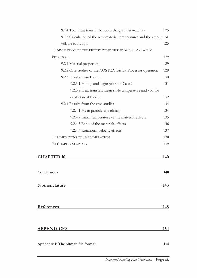
Shear mixing, as the name suggests, occurs due to the shear stresses being applied to
the solid bulk of a granular material. These stresses concentrate at slipping planes and
when these stresses exceed the inter particle frictional forces, the granular materials
move relative to each other (Bridgewater, 1976). This results in a bulk relocation of
some of the granular material and provides bulk mixing as shown by an increase of
the contact between the two different coloured regions at the slipping plane, each
representative of a different material, in Figure 2.1. The thick inclined line in Figure
2.1 shows the location of the slipping plane.
Figure 2.1:Shear mixing of a granular material.
2.1.2 Convective mixing of granular materials
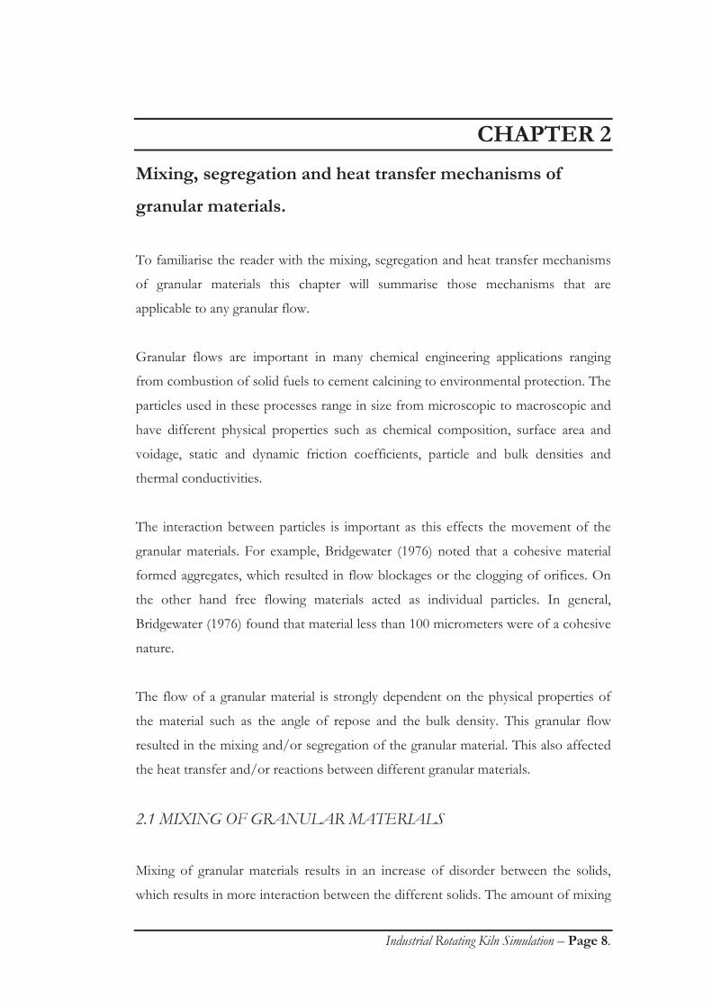
Convective mixing is also a bulk mixing mechanism and occurs as a result of the
velocity gradients within granular materials (Cahn & Fuerstenau, 1967; Hogg &
Fuerstenau, 1972).
The shear rates between different layers of particles result in the layers sliding over
each other as shown in Figure 2.2. By definition, convective mixing is fully reversible
since there is no random distribution of the materials during the convective mixing
process. Hogg & Fuerstenau (1972) described the convective mixing in a rotating
drum at low speeds.

Industrial Rotating Kiln Simulation – Page 11.
Figure 2.2:Convective mixing of a granular material.
2.1.3 Diffusive mixing of granular materials
Diffusion was described by Hogg et al (1966) and Cahn & Fuerstenau (1967) to
conform to the one dimensional form of Fick’s second law of diffusion which states
that the diffusion mixing process is completely random, similar to the diffusion
process in liquids or gases and is given by:
xtxCD
xttxC
Diff),(),( (2.2)
where C(x,t) is the concentration at any time, t, and distance, x, from the original
surface and DiffD is the diffusion coefficient. The solution to Fick’s second law was
presented by Hogg et al (1966) and can be used to predict the relative concentrations
of a mixture at any point and any time.
Cahn & Fuerstenau (1967) defined diffusion mixing as “micromixing” where the
individual particles diffused across boundaries between regions rich in one
component into regions rich in another component. Zik & Stavans (1991) found that
an oscillating velocity in a bed of particles resulted in self diffusion of the materials in
the bed. Kohring (1995) showed that the self diffusion coefficient of the materials
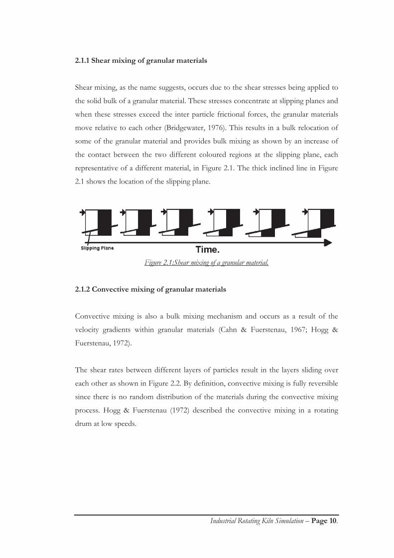
increased as the magnitude of the oscillating velocity increased. Figure 2.3 illustrates
the diffusive mixing mechanism of an initially separated material subjected to an
oscillating horizontal velocity.
Industrial Rotating Kiln Simulation – Page 12.
Figure 2.3: Diffusive mixing of a granular material subject of an oscillating horizontal velocity.
2.2 SEGREGATION OF GRANULAR MATERIALS
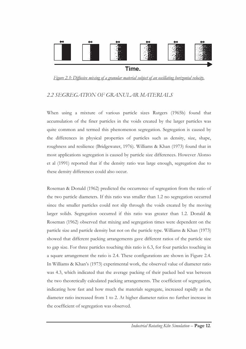
When using a mixture of various particle sizes Rutgers (1965b) found that
accumulation of the finer particles in the voids created by the larger particles was
quite common and termed this phenomenon segregation. Segregation is caused by
the differences in physical properties of particles such as density, size, shape,
roughness and resilience (Bridgewater, 1976). Williams & Khan (1973) found that in
most applications segregation is caused by particle size differences. However Alonso
et al (1991) reported that if the density ratio was large enough, segregation due to
these density differences could also occur.
Roseman & Donald (1962) predicted the occurrence of segregation from the ratio of
the two particle diameters. If this ratio was smaller than 1.2 no segregation occurred
since the smaller particles could not slip through the voids created by the moving
larger solids. Segregation occurred if this ratio was greater than 1.2. Donald &
Roseman (1962) observed that mixing and segregation times were dependent on the
particle size and particle density but not on the particle type. Williams & Khan (1973)
showed that different packing arrangements gave different ratios of the particle size
to gap size. For three particles touching this ratio is 6.3, for four particles touching in
a square arrangement the ratio is 2.4. These configurations are shown in Figure 2.4.
In Williams & Khan’s (1973) experimental work, the observed value of diameter ratio
was 4.3, which indicated that the average packing of their packed bed was between
the two theoretically calculated packing arrangements. The coefficient of segregation,
indicating how fast and how much the materials segregate, increased rapidly as the
diameter ratio increased from 1 to 2. At higher diameter ratios no further increase in
the coefficient of segregation was observed.

Industrial Rotating Kiln Simulation – Page 13.
Figure 2.4:Different packing arrangements showing the difference in particle size to gap size: a)
diameter ratio = 6.3, b) diameter ratio = 2.4 (Williams & Khan, 1973).
Segregation within a granular flow occurred via a combination of the percolation,
flow and vibration mechanisms (Nityanand et al, 1986). These mechanisms are
described below.
The darker particles in Figures 2.5 to 2.7 represent segregating particles as they
segregated. The larger white particles represent the larger particles in the bed of
solids.
2.2.1 Percolation segregation mechanism of granular materials
Percolation segregation occurs when smaller particles pass through the voids
between the larger particles to accumulate beneath the larger particles. Williams &
Khan (1973) stated that percolation segregation depended on “the probability that a
particle will find a void into which to fall”. This probability depends on the size of
the particles and the particle size ratio. The most common occurrence of percolation
segregation occurs in the pouring of heaps of multi sized particles and this is referred
to as free surface segregation. The process of free surface segregation involves the
percolation of the finer particles in the voids of the bed and the sinking of the
heavier particles due to their larger relative weight as shown in Figure 2.5 (Alonso et
al, 1991). The dark filled circles of Figure 2.5 to 2.7 represents the segregating

Industrial Rotating Kiln Simulation – Page 14.
particle. The smaller heavier particles end up at the bottom of the bed and the larger
lighter particles end up at the top of the bed. Alonso et al (1991) derived a
correlation, which can be used to calculate an appropriate density ratio to
compensate for the percolation segregation mechanism so that the mixture will not
segregate.
Figure 2.5:Percolation segregation of a granular material.
Spontaneous segregation occurs when the finer material segregates through a
stationary bulk of larger particles (Bridgewater, 1976). The gravitational force acting
on the fine particles is sufficient to allow the fine particles to fall through the voids
created between the larger particles.
2.2.2 Flow or trajectory segregation mechanism of a granular material
When particles are projected across a surface the distance they travel along this
surface is proportional to the square of the particle diameter (Williams & Khan,
1973). This indicates that a larger particle travels further compared to a smaller
particle as shown in Figure 2.6. This occurs because the smaller particles are captured
more readily by the inclined plane due to the increased relative contact area of the
smaller particles and this increases the dynamic friction for these particles thereby
reducing their velocity.
Figure 2.6:Flow segregation of a granular material.

Industrial Rotating Kiln Simulation – Page 15.
2.2.3 Vibration segregation mechanism of a granular material
The final possible segregation mechanism is vibration segregation. Vibration
segregation occurs when a bed of particles is vibrated. The larger particles rise to the
surface even if they are denser than the finer particles (Williams & Khan, 1973). This
is illustrated in Figure 2.7.
Figure 2.7:Vibration segregation of a granular material.
2.3 HEAT TRANSFER IN GRANULAR MATERIALS
Heat transfer in a granular medium occurs through a combination of conduction,
convection, radiation and advection (Arpaci, 1966). The relevance of each of these
heat transfer mechanisms depends on the nature of the granular material. Radiation
heat transfer is important for particles greater than 1 mm diameter or at a
temperature of more than 400°C (Saatdjian & Large, 1988). Under these conditions,
Yagi & Kunii (1957) and Schotte (1960) reported that radiation could account for up
to 80% of the total heat transfer. Molerus (1997) showed that there is negligible
contact between large hard particles indicating that conduction heat transfer between
such particles is negligible.
2.3.1 Heat transfer paths between particles
Heat transfer between solid particles has been described by Yagi & Kunii (1957) and
Kunii & Smith (1960). Figure 2.8 illustrates the different paths of heat transfer
between particles. Heat transfer path 1 is the conduction heat transfer between the
particles through the points of contact between the particles. Path 2 is the heat
transfer by conduction and convection through the fluid film near the place of

Industrial Rotating Kiln Simulation – Page 16.
contact. Heat transfer path 3 is the net radiation heat transfer from the surface of a
hot particle to the surface of cold particle. Radiation from the hot particle to the void
space between particles and radiation from the void space to the cold particle are
described as paths 4 and 5, respectively. Lastly path 6 describes the heat transfer
from the surface of the cold particle into the bulk of the colder particle due to
conduction. The total heat transfer through all six paths, Q, to the cold particle can
be described as:
TUAQ (2.3)
where U is the overall heat transfer coefficient, A is the heat transfer area of the
particle and T is the temperature difference between the particles.
Figure 2.8; Heat transfer paths between particles (Yagi & Kunii, 1957).
Rao & Toor (1984, 1987) studied the effects of size and thermal conductivity ratios
on the heat transfer from a particle to a surrounding bed of particles. They found
that the discrete nature of the particle diminished as the conductivity ratio was
decreased or the particle size ratio was increased. Under these conditions, the heat
transfer from the particle could be considered as heat transfer from the particle to a
continuum. However, the discrete nature of the particles must be considered if the

Industrial Rotating Kiln Simulation – Page 17.
test particle was of similar size to the bed particles. Their discrete model to determine
the heat transfer coefficient from their test particle to the bed of particles included a
measurement for the number of contacts between the test particle and the particles
in the surrounding bed.
Saadjian & Large (1988) indicated that the heat transfer between larger particles at
elevated temperatures occurred predominantly through radiation. When a gaseous
medium was used, convection between the stagnant fluid and the particles was small
due to the lower thermal conductivity of the gases compared to that of solids.
2.3.2 Heat transfer in a granular medium
A granular medium can be described as numerous particle-particle interactions and
the heat transfer in a granular medium occurred through these interactions. The
effective thermal conductivity of the granular medium has been used to determine
the heat transfer to the granular medium (Schotte, 1960; Dixon & Cresswell, 1979).
Yagi & Kunii (1957) calculated the effective thermal conductivity, ke0, of a stationary
medium. In a moving medium the effective thermal conductivity of the granular
medium, ke, includes a transport term so that:
teee kkk 0 (2.4)
where ket was the effective thermal conductivity dependent of the fluid flow. Yagi &
Kunii (1957) included the mean particle diameter and the radiative heat transfer in
their thermal conductivity determination. Kunii & Smith (1960) found that there was
a decrease in thermal conductivity with an increase in void fraction. Barker (1965)
found that bed packing directly affected the bed voidage and the contact between the
particles. Since fine dusts can have a voidage of up to 98% the presence of fine dusts
in poorly packed beds could results in a decrease of the thermal conductivity of the
granular medium.
Gurgel & Kluppel (1996) studied the heat transfer in a granular medium by changing
the moisture content of the voidage between particles. They found that the bed

Industrial Rotating Kiln Simulation – Page 18.
thermal conductivity was strongly dependent on the voidage composition. This
indicated that the heat transfer in a granular medium was limited by the thermal
conductivity of the fluid in the voids of the granular medium. This is especially
important at lower temperatures where the radiation heat transfer is not dominant.
Furthermore, Hunt (1997) also found that the fluid phase properties of a granular
medium are critical in the heat transfer since the particles exchanged most of their
heat with the fluid. This is especially important if the fluid is a gas since thermal
conductivities of gases are much lower compared with thermal conductivities of
solids thereby limiting the heat transfer rate.
Granular materials have been used to dry fruits and grains due to the enhanced
conduction between solids because of the larger thermal mass of solid materials
compared to air. This heat transfer mechanism was referred to as granular medium
heat transfer. Raghavan et al (1974) found that using granular materials had the
advantage of being economical and provided a uniform heat transfer from one
material to the other depending on the mixing conditions of the granular medium.
Sullivan et al (1975) found that the increase in thermal mass, compared with gaseous
heating, resulted in shorter drying times and reduced overheating of the material to
be dried.
Particulate medium heating is the method of heat exchange between the solids in the
AOSTRA-Taciuk Processor. However in the AOSTRA-Taciuk Processor, the
operating temperatures are significantly higher than those experienced in previous
particulate medium heating systems and thus the heat transfer mechanism between
the materials will be different.
2.4 CHAPTER SUMMARY
The movement of granular materials, namely the mixing and segregation mechanisms were
introduced as well as the heat transfer characteristics of granular materials. Practical applications of
mixing and/or segregation in rotating kilns are described in Chapter 3. Discussion of the heat
transfer between particles will be expanded in Chapter 9 where the simulation of the AOSTRA-

Industrial Rotating Kiln Simulation – Page 19.
Taciuk Processor, including heat transfer between the different particles and the volatile evolution will
be carried out.

Industrial Rotating Kiln Simulation – Page 20.
CHAPTER 3
Rotating drums and kilns – literature review.
In this chapter, the literature characterising the operations of a rotating drum is
reviewed. This is then extended to include studies of the mixing, segregation and heat
transfer of solids in rotary kilns.
The movement of solids in a rotary kiln consists of both a transverse and an axial
component. The axial movement is defined as the movement parallel to the axis of
the rotating drum whereas the transverse component occurs perpendicular to the
axis. Barr et al (1989a, b) found that the transverse movement was important to
obtain a homogenous bed. On the other hand, Perron & Bui (1990) noted that the
axial movement was important for predicting the overall residence times of the solids
in the kiln. Pershin & Minaev (1989a) believed that the intensity of heat and mass
transfer depended to a great extent on the type of motion experienced in the
transverse section of a rotating drum.
The literature shows that modelling of rotary kilns has been limited to either
modelling in the transverse direction or the axial direction. Modelling to date includes
flow, mixing, segregation and heat transfer in either the transverse or axial direction.
The mixing and segregation models in the past have been mostly qualitative and
focused on calcining kilns where the heat transfer occurs from the gaseous phase
above the bed to the bed of solids. There is a lack of quantitative knowledge of the
industrial rotary kiln especially with respect to the proposed AOSTRA-Taciuk
Processor, which was described in Chapter 1.
Eventhough the focus of this thesis is the transverse motion of a rotating drum, it is
relevant to discuss the axial motion since most industrial rotating kilns have high
length to diameter ratios. The time spent travelling through the kiln is important
from both an operational and economic point of view and is dependent upon the
axial flow in the kiln.

Industrial Rotating Kiln Simulation – Page 21.
3.1 TRANSVERSE MOTION IN A ROTATING DRUM
3.1.1 Transverse bed regimes
Henein et al (1983a, b) described six different motion regimes in the transverse
direction of a rotating bed as shown in Figure 3.1. The motion of the bed was shown
to depend on the rotational velocity of the rotating drum and is commonly expressed
as a function of the Froude number. The Froude number, Fr, is the ratio of
centrifugal to gravitational forces and can be calculated using equation 3.1;
gRFr2
(3.1)
where is the rotational velocity in rad s-1, R is the radius of the drum in m and g is
the acceleration due to gravity in ms-2.
Figure 3.1 Different motion regimes in a rolling drum (Henein et al, 1983a, b).
At low speeds and low loading, Henein et al (1983a, b) showed that the bed
“slipped” continuously. This was due to the low friction between the solids and the

Industrial Rotating Kiln Simulation – Page 22.
drum walls, and resulted in minimal movement of the solids with respect to each
other. At slightly higher speeds the bed passed through a “slumping” stage. When
the potential energy of the material in the upper triangle, as shown in Figure 3.1b,
exceeds the static inter-particle forces this material flows into the area indicated by
the lower triangle. This slumping occurred periodically. Increasing the velocity
further resulted in a “rolling” bed where the solid material continuously moved
upward with the drum walls and rolled down the inclined surface, as shown in Figure
3.1c. “Cascading” is a more severe form of rolling and this occurs at slightly higher
velocities where the upper surface of the bed became more wavelike. “Cataracting”
occurs when solids at the high point of the bed became airborne due to the extra
kinetic energy of the particles as they left the free surface of the bed. This was
beneficial for extra gas-solid contact and was simulated at lower velocities using
flights on the inside surface of the rolling drum. Papadakis et al (1994), Baker (1992)
and Sherritt et al (1993, 1994) termed their cataracting regime as cascading even
though this did not follow the cascading regime as described here. “Centrifuging”,
shown in Figure 3.1f, occurs when the kiln is rotating at a velocity greater than the
critical speed. In this regime all the solids adhered to the wall and formed an annulus.
The critical rotational speed of a rotational drum, c, can be calculated using:
Rg
c (3.2)
The Froude number equals 1 at the critical rotational speed (Henein et al, 1983a)
since the centrifugal forces balance the gravitational ones. Rolling of the bed
occurred when the rotational speed was greater than 0.10 c and less than 0.55 c.
Rutgers (1965a) found that cataracting occurred in the region of 0.55 to 0.60 c.
Rolling, cascading and cataracting are the most common motion regimes since they
provide good relative material movement. The focus of this research is on the
transverse rolling regime, which will be described in the next section.
Henein et al (1983a, b) constructed “Bed Behaviour Diagrams” for different solids
under different conditions in order to describe the motion regime of the solids bed.
The “Bed Behaviour Diagrams” for the different materials are qualitatively similar.
They found that nodular material rolled at lower rotational velocities compared to
Industrial Rotating Kiln Simulation – Page 23.
irregular particles and that smaller particles rolled at higher rotational rates due to the
extra interfacial area resulting in higher friction coefficients. These “Bed Behaviour
Diagrams” could be used to predict the regime of the bed from the operational
variables such as the rotational speed, the drum loading and the particle
characterisation.
Pershin & Minaev (1989a) studied these transverse bed regimes and found that the
mixing regime of the bed was dependent on the potential energy of the material in
the bed.
3.1.2 The transverse rolling regime in a rotating drum
The rolling regime was described and observed by Lehmberg et al (1977) to consist
of two layers, namely the active and stagnant layers. The stagnant layer was
considered as a dense plug, which moved at the same rotational velocity as the wall
due to the no slip boundary condition between the bed of solids and the wall. The
active layer occurred when particles moved relative - down the incline - to each other
resulting in both mixing and segregation. This regime has been studied in detail due
to its importance in rotating kiln operation.
3.1.2.1 Description of the active layer in the rolling regime
Different active layer geometries, as shown in Figure 3.2, have been used in the past.
Lehmberg et al (1977) observed that the active layer in a rolling bed was curved and
occupied a certain percentage of the bed height. Mu & Perlmutter (1980) and
Woodle & Munro (1993) considered the active layer as a layer of uniform thickness
at the free surface of the rolling bed where the mixing occurred. Ferron & Singh
(1991) considered the active layer as a very fast moving layer being a single particle
thick at the top of the stagnant layer.

Industrial Rotating Kiln Simulation – Page 24.
Figure 3.2: Active layer configurations; A) Lehmberg et al (1977), B) Mu & Perlmutter (1980),
Woodle & Munro (1993), C) Ferron & Singh (1991).
Nakagawa et al (1992) measured the transverse velocity profile using magnetic
resonance imaging. They observed that the velocity profile in both the active layer
and stagnant layers were linear. The transverse velocity profile was confirmed by
Boateng & Barr (1997) who measured the velocities of particles moving away from
an optical probe. These experiments showed that the active layer thickness of a
rolling bed could be approximated by a fraction of the bed height similar to the
geometry used by Lehmberg et al (1977). This fraction depends on the granular
material properties and the experimental conditions. Furthermore, Boateng (1993)
observed that the velocity profile in the active layer of larger beds was skewed
indicating that the material was still accelerating past the mid chord position and
would not result in a symmetric velocity profile about the mid chord position. This
has important implications in determining the solid behaviour in larger drums since
more movement occurs between the particles in the lower section of the active layer
compared to the movement in the upper section of the active layer. Figure 3.3
illustrates the velocity profile at mid chord in a rolling bed as observed by Nakagawa
et al (1992) and Boateng & Barr (1997). The linear velocity gradients of both the
active and stagnant layer are indicated on the figure. A mean velocity of each layer is
also shown in the figure. As can be seen from the figure, the mean velocity in the
active layer is significantly larger than the mean velocity in the stagnant layer and this,
combined with the less dense packing of the active layer, results in the mixing and/or
segregation of solids in the bed.

Industrial Rotating Kiln Simulation – Page 25.
Figure 3.3: Rolling bed velocity profile (Nakagawa et al, 1992; Boateng, 1993).
The active layer depth was often considered as the proportion of the mid chord bed
height occupied by the active layer. Cahn et al (1967) observed a “dead” zone in the
transverse section when the bed was filled so that it exceeded 50% of the cylinder
volume. Hogg & Fuerstenau (1972) removed this “dead” zone by increasing the
velocity of the kiln so that the active layer proportion increased and the centre of
rotation of the bed was forced below the centre of the “dead” zone. This early work
showed that the active layer depth was dependent upon the rotational velocity. In
their experimental study of transverse bed motion, Henein et al (1983a, b) noted that
the active layer depth decreased for smaller particles, decreased with bed depth and
increased with rotational speed. In further work Henein et al (1985) indicated that
the fine proportion of the bed did not affect the size of the active layer. Boateng
(1993) found that the active layer proportion with respect to bed depth increased
with increasing rotational speed and decreased with bed loading. Yang & Farouk
(1997) modelled the flow field of a rolling bed in a rotary kiln. At mid chord, their
active layer depths were approximately 40-50 % of the bed height for all their
experiments. They also measured the velocity profile for different sized particles and
found that the active layer thickness increased for smaller particles, but the velocity
gradient was not as steep. This was contradictory to the work of Henein et al (1983a,

Industrial Rotating Kiln Simulation – Page 26.
b) and was probably due to the use of different granular materials and different
experimental conditions. This emphasised that granular materials were not easily
classified and that the behaviour of solid materials should be characterised prior
using them in experimental studies.
Rutgers (1965b) measured voidages of the active layer between 0.50 and 0.55. Mu &
Perlmutter (1980) showed that the initial velocities of particles entering the active
layer are dependent upon the position at which the particles entered the active layer.
The large voidages and the different velocities of particles resulted in the mixing
and/or segregation of the solids as they passed through the active layer according to
the mechanisms described in Chapter 2.
Donald & Roseman (1962) and Nityanand et al (1986) showed that measurements at
the end surface of a rotating drum were not representative of the bulk of the drum.
They found that the end effects were limited to a few particle diameters from the end
of the drum. Boateng & Barr (1997) found that the end surface effect increased the
angle subtended by the material by approximately 10% over that of the undisturbed
region. This resulted in velocity enhancement of the particles in the active layer near
the end surface. Due to this increased velocity of 20-25%, the active layer depth was
observed to be smaller, by approximately 15%, at the end surfaces compared to the
bulk. This end effect needs to be accounted for to fully model the behaviour of
solids in a rotating bed. Thus, experimental results obtained through a transparent
end surface included the end effects and needed to be corrected in order to predict
the motion and mixing parameters within the bulk of the bed.
3.1.2.2 Description of the stagnant layer in the rolling regime
The stagnant layer has not been characterised to the same extent as the active layer.
Rutgers (1965) measured the density of a bed of cereal grains to be approximately
70% of the loosely packed bulk density of the material. This bulk density decreased
as the rotational velocity increased. The bulk phase of the rolling bed provided
intimate particle-particle contact which was of great importance when heat or mass
transfer was required within the bulk phase (Ferron & Singh, 1991). This showed the

Industrial Rotating Kiln Simulation – Page 27.
importance of the bulk phase, which in most cases was considered as a moving
packed bed.
3.1.2.3 Description of the mixing and segregation in the rolling regime
Mixing and segregation are two facets of the same physical process, namely granular
flow. Since these processes are strongly linked and occur simultaneously, they will
both be described together in this part of the thesis. This review is given in a
chronological order and is concluded with a final paragraph to summarise the
important findings.
Roseman & Donald (1962) showed that transverse mixing decreased as the bed
height increased and that transverse mixing was slow. However, Rutgers (1965a, b)
clearly stated that the mixing in the transverse direction was 2 to 4 orders of
magnitude faster than mixing in the axial direction. Rutgers (1965a, b) found that
most of the mixing in a rolling bed takes place in the bottom part of the active layer
and that the extent of this mixing was determined more by the total number of
revolutions rather than the velocity of the drum.
Hogg & Fuerstenau (1972) described the convective mixing mechanism, as described
in Chapter 2, for a rotating drum. The convective mixing component can only be
studied at low rotational velocities. Convective mixing occurs in a rolling bed due to
the differences in particle circulation times. These differences occur when the
particles re-enter the stagnant layer in the same circulation zone as the one they
emerged from. In the stagnant layer, the residence times of the particles in all the
circulation zones were equal. However the time spent in the active layer depended on
the distance the particles traveled across this active layer. For the particles rotating
closer to the wall, they need to travel a greater distance and as they travel further
down the inclined plane their circulation period would be prolonged. In the
meantime other particles closer to the centre had already re-entered the stagnant
layer. This resulted in the formation of thinner and thinner bands as more rotations
were experienced and eventually led to a system of numerous parallel thin bands.
This is shown in Figure 3.4. Convective mixing as described here only occurred in
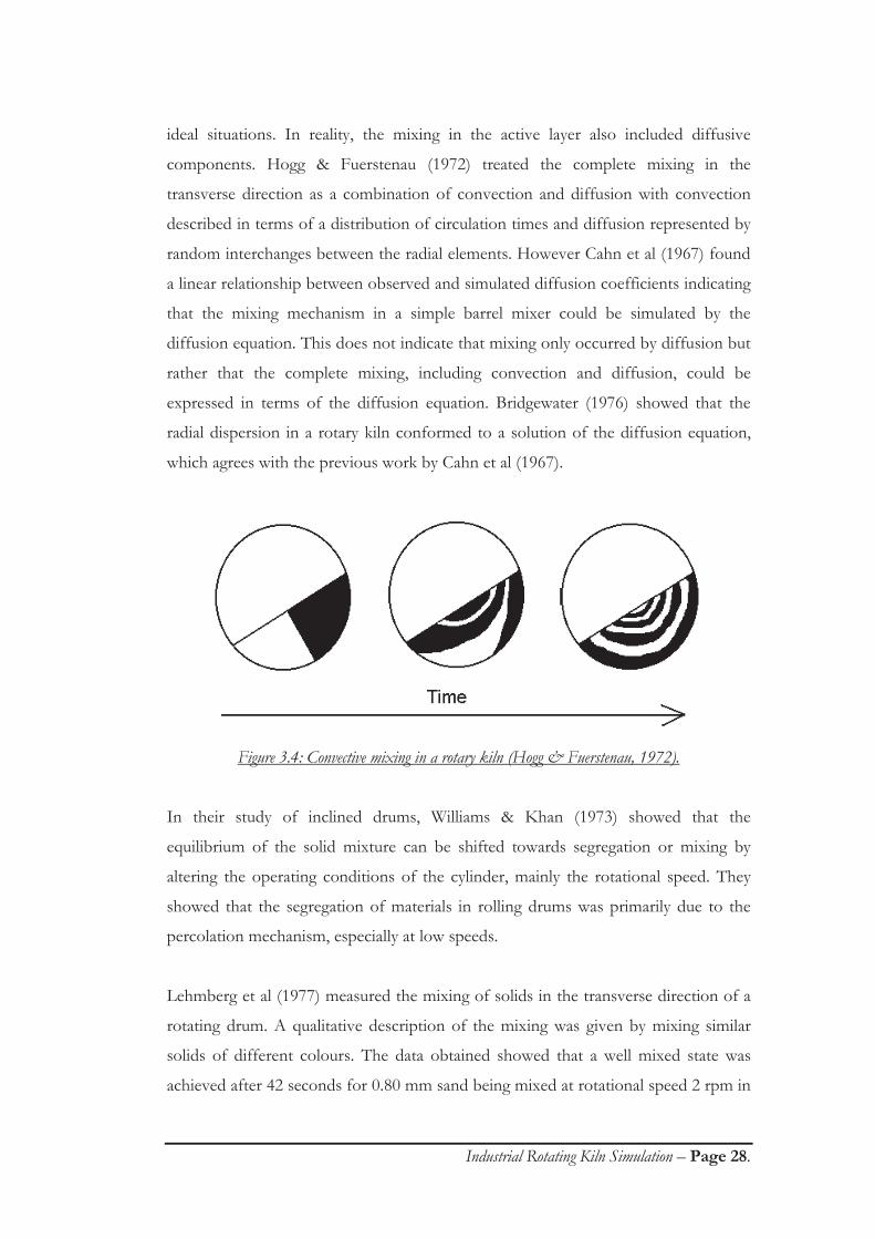
Industrial Rotating Kiln Simulation – Page 28.
ideal situations. In reality, the mixing in the active layer also included diffusive
components. Hogg & Fuerstenau (1972) treated the complete mixing in the
transverse direction as a combination of convection and diffusion with convection
described in terms of a distribution of circulation times and diffusion represented by
random interchanges between the radial elements. However Cahn et al (1967) found
a linear relationship between observed and simulated diffusion coefficients indicating
that the mixing mechanism in a simple barrel mixer could be simulated by the
diffusion equation. This does not indicate that mixing only occurred by diffusion but
rather that the complete mixing, including convection and diffusion, could be
expressed in terms of the diffusion equation. Bridgewater (1976) showed that the
radial dispersion in a rotary kiln conformed to a solution of the diffusion equation,
which agrees with the previous work by Cahn et al (1967).
Figure 3.4: Convective mixing in a rotary kiln (Hogg & Fuerstenau, 1972).
In their study of inclined drums, Williams & Khan (1973) showed that the
equilibrium of the solid mixture can be shifted towards segregation or mixing by
altering the operating conditions of the cylinder, mainly the rotational speed. They
showed that the segregation of materials in rolling drums was primarily due to the
percolation mechanism, especially at low speeds.
Lehmberg et al (1977) measured the mixing of solids in the transverse direction of a
rotating drum. A qualitative description of the mixing was given by mixing similar
solids of different colours. The data obtained showed that a well mixed state was
achieved after 42 seconds for 0.80 mm sand being mixed at rotational speed 2 rpm in
Industrial Rotating Kiln Simulation – Page 29.
a 300 mm diameter drum. This was quantified using hot tracer particles and then the
temperature was measured at the top of the bed. The temperature of the bed at this
position followed an exponential oscillating decay with respect to the maximum
temperature. The rate of mixing was not calculated by the authors but could be
determined from the successive peaks by considering the heat transfer from the hot
particles to the colder particles. This work did not determine the effects of changing
experimental variables.
Henein et al (1985) observed that vibration segregation was not applicable to rotary
kilns, instead segregation in rotary kilns is governed by the percolation mechanism,
which is in agreement with the observations of Williams & Khan (1973).
Nityanand et al (1986) measured transverse segregation to occur within 1 to 10 bed
revolutions whereas axial segregation took from 500 to 10000 bed revolutions for
complete segregation. This order of magnitude difference between transverse and
axial solid movement mechanism is quite often observed, not only for segregation
but also for mixing. Furthermore, in the vicinity of the walls, such as in any visual
experiment, the end wall effects decreased the size of the segregated core. As
previously mentioned Boateng (1993) found that the velocity in the active layer
increased near the walls. Combining these two results indicates that segregation
decreases with increased velocity. Nityanand et al (1986) also showed that particles in
the segregated core are restricted to the segregated core as shown in Figure 3.5.
Pollard & Henein (1989) showed that transverse segregation followed zero order
kinetics and expressed the segregation behaviour as a normalised segregation rate.
The initial content of fines in the bed did not effect the normalised segregation rate
however a linear dependence on rotational speed was observed. The size ratio did
effect the segregation rate, whereas bed depth did not effect the segregation rate.
Pollard & Henein (1989) compared segregation rates of irregular limestone particles
to smooth acrylic spheres and found these segregation rates to be similar. This
indicates that the segregation rate is independent on the particle size and particle
friction. This point was not adequately explained in the literature and illustrates the
need for further research to study the behaviour of solids in rotating drums. Pollard

Industrial Rotating Kiln Simulation – Page 30.
& Henein (1989) showed that the segregated core was of similar shape as the rotating
bed and that the segregated core formed near the middle bottom of the active layer
as shown in Figure 3.5.
Figure 3.5: Schematic of the segregated core.
Pershin & Minaev (1989a, b) studied the mixing and segregation of a granular
material in the transverse section of a rotary drum using the concentric sublayer
model that was developed by Pershin (1987). Mixing or segregation was assumed to
occur if the material moved from one sublayer to an adjoining one, only one
transgression was permitted per bed revolution. This was not consistent with
observations that segregation sometimes occurred within a single bed revolution,
which required the movement of fines through numerous layers per bed revolution.
Mixing occurred when a particle left its zone of circulation. Segregation occurred in a
similar manner but with the added constraints of movement closer to the center of
rotation and that the particle remained trapped in this new circulation zone. Mixing
also occurred through the re-arrangement of particles within any sublayer but this
was not considered by Pershin & Minaev (1989a, b).
Woodle & Munro (1993) measured mixing dynamics for ovoid, shell and tube solids
from 3 to 15% loading in a rotating drum using a statistical method where the
concentrations of the top and bottom surfaces of the bed were measured. These

Industrial Rotating Kiln Simulation – Page 31.
experiments indicated that mixing occurred 10 times faster when strips were attached
to the inside walls of the drum compared to a rolling drum without strips. Previous
work by Wes et al (1976a, b) also showed that the transverse mixing coefficient
increased with rotational velocity and normal strip height. Mixing times of 46
minutes were measured by Woodle & Munro (1993) for shell shaped particles with a
rotational speed of 8.5 rpm. These times were much larger than those observed by
Lehmberg et al (1977) even though a higher rotational velocity was used. This lack of
agreement clearly indicates the need of further research into this area. Woodle &
Munro (1993) derived a correlation to determine the time required to obtain a fully
mixed condition using the complete mixing time of a certain material and the ratio of
friction factors of the two materials: 3.1
2
1
2
1
tt
(3.3)
where t1 and t2 were the respective mixing times and 1 and 2 were the friction
coefficients of the material. This equation is only applicable for the same
experimental conditions with different materials. The mixing dynamics in these
experiments were at a constant rate until the steady state was reached. A random
distribution was observed at the end of mixing due to the stochastic nature of
mixing.
A combined model of mixing and segregation was developed by Boateng & Barr
(1996a) for a binary mixture. This model calculated the concentrations of “flotsam”
and “jetsam” in a series of control volumes and from this the movement of particles
were calculated with respect to bulk flow, diffusion and segregation. This model
required the knowledge of concentration gradients across the bed, segregation flux
coefficient and the diffusion coefficient. The focus of the work by Boateng & Barr
(1996a) was on the segregated bed and the heat transfer from the gas phase to the
solid bed, which has important implications in calcining kilns but was not so helpful
for the mixing and heat transfer between the granular material. The dynamics of
mixing and segregation were not modelled and the model was only effective for the
prediction of the final distribution of particles in a rolling bed.

Industrial Rotating Kiln Simulation – Page 32.
The effect of mass ratio on segregation was studied by Ristow (1994) using equal
sized particles of different densities. It was shown that the segregation velocity
increased proportionally with the logarithm of the mass ratio of the particles.
Furthermore, as this mass ratio was increased the final circulation zone of the
segregated material was closer to the rotating centre of the bed. Significant density
ratios were required to create a segregated core.
Clément et al (1995) carried out segregation work in a two dimensional experiment.
They simulated the segregation by tracing the position of a single particle in a thin
transverse section. A core was formed when the tracer particle was smaller than the
bed particles. A trace close to the wall was formed when the tracer particle was
larger than the bed particles. Perfect distribution of the tracer particle was observed
when the tracer particle was the same size as the bed material. It should be noted that
in their experimental work the bed material consisted of 1.5 mm steel spheres and
the tracer particles were 1.0, 1.5 and 2.0 mm spheres respectively. The operating
regime of the bed was the rolling regime, which they described as the rotational
velocity where a surface avalanche started. For their 160 mm inner diameter cylinder
and approximately 40% loading, this velocity was 1/3 rpm. Furthermore they
proposed a parameter to characterise the segregation. This was the typical
segregation length with a sign indicating the direction of segregation, i.e. towards or
away from the centre of the bed as illustrated in Figure 3.3. This correlation needs to
be further investigated since it only involved three particle sizes and no changes in
particle densities or friction coefficients.
Cantelaube et al (1997) expressed the extent of segregation by an order parameter P0,
which was a measure of the normalised area of the segregated material in a reference
cluster. This parameter equalled 1 for a fully segregated system and 0 for a
homogenous system. The order parameter as a function of time, P0(t), was: t
etP 1)(0 (3.4)
where t was the time passed and characterised the kinetics of segregation. From this
correlation it was shown that the segregation time constant was independent of the
concentration of fines. Furthermore, Cantelaube et al (1997) stated that the

Industrial Rotating Kiln Simulation – Page 33.
segregation time constant was not dependent on the rotational velocity. It was quite
unclear what was meant since this was contradictory to the experimental results of
Williams & Khan (1973) and Pollard & Henein (1989) who showed that segregation
was dependent upon the rotational velocity of the drum. The segregation was
observed to be very fast, with a nearly complete segregated cluster forming within a
single drum revolution. The core formation and rapid segregation was in agreement
with the results from Pollard & Henein (1989). Cantelaube et al (1997) described the
active layer as a fluctuating sieve allowing the smaller particles to percolate causing
segregation.
In summary, a number of studies have been reviewed in this section of the thesis.
Much of this work was carried out to determine the mixing and segregation in the
transverse section of a rolling bed. Various models available but each has its own
designated purpose. Most of the models in the literature are only qualitative and
there is significant disagreement between the results of various authors. This
indicates that more research is required in this area, especially with respect to
quantifying the mixing and segregation and relating the models back to various
operational parameters of a rotating kiln.
3.2 AXIAL MOTION IN A ROTATING DRUM
Models of motion in the axial direction of a rotary kiln often assume that the bed is
perfectly mixed, or isothermal in heat exchange calculations, across any transverse
section. This assumption was applicable since the radial dispersion was many
magnitudes of order greater than the axial dispersion (Kelbert & Royere, 1991).
3.2.1 Motion in the axial section of a rotating drum
Pickering et al (1951) observed that the movement of particles down the inclined
plane of a rotary drum was strongly influenced by the friction of the bed. Solid
movement in a rotary kiln was due to the horizontal inclination of the top surface of
the bed. Kramers & Crookewit (1952), Hogg et al (1974) and Kelbert & Royere
(1991) reported that the axial motion can be represented as a slow plug flow in the

Industrial Rotating Kiln Simulation – Page 34.
stagnant zone and it was shown that material passes along the axis due to the solids
rolling at an incline from the top surface. The resulting combination of transverse
motion and movement of particles down the axial incline results in the particles
following a pseudo helical trajectory as shown in Figure 3.6.
Figure 3.6: Schematic illustrating the pseudo-helical trajectory of particles through a rotary kiln.
A general relation to determine the axial velocity was derived by Perron & Bui
(1990), by considering the bed as a continuum, with the only unknown parameter
being the apparent viscosity of the bed. This predicted the average axial velocity but
cannot be used to determine the velocities of individual particles in different paths.
Boateng & Barr (1996a) considered the axial flow as a constant flux that only
occurred in the active layer as the stagnant layer was densely packed. In subsequent
work, Boateng & Barr (1997) found that axial motion was influenced by the active
layer depth and the drum rotational velocity.
The elutriation of fines from a rotary kiln may be significant if a large gas phase
velocity was used. Fines elutriation was studied by Tackei et al (1989, 1990) and may
have important implications for the elutriation of particles from the top surface of
the bed, especially in the case of a gas fired kiln due to the high gaseous volumetric
throughput.
3.2.2 Residence times in rotating kilns
The residence time in a rotary kiln was determined from the rate of axial transport in
the kiln, which in turn is dependent upon the rotational velocity of the kiln.

Industrial Rotating Kiln Simulation – Page 35.
Predictions of residence times are important for quality control of the products.
Axial transport in the rotary kiln closely resembles plug flow as shown by the tracer
experiments of Pickering et al (1951), Rutgers (1965a, b), Ray et al (1994) and Sze et
al (1995). A tracer experiment generally involved charging the rotary drum with a
certain type of material. After the solids flow in the kiln was well established the feed
was changed to a new material with different visual properties but similar
characteristics such as size, density and friction. Usually only a pulse of the different
material was considered. In order to compare residence times under various
conditions, three parameters were suggested by Sai et al (1990). These were the mean
residence time of the pulse of solids, the variance and the skewness of the residence
time distribution. Rutgers (1965b) reported that for a slumping bed the residence
time was 1.7 times that of a rolling bed. However this figure should only be used as
an approximation since there is a wide range of rolling velocities.
The residence time of solids in a rotating drum was found by Pickering et al (1951) to
be dependent on the inclination of the drum, the rotational speed of the drum and
the material flow rate. An increase in the rotational velocity resulted in a decrease of
the measured residence time in the rotary kiln (Lebas et al, 1995).
Pickering et al (1951) and Hogg et al (1974) observed that the residence times of
smaller particles were longer than for larger particles due to the segregation of the
smaller particles. These segregated particles travelled through the kiln at a slower
axial velocity. Lebas et al (1995) also observed this behaviour for finer material.
Most of the time of passage determinations were not valid for rotary kilns with
restricted discharge ends. The effect of the addition of such constrictions was
estimated by Saeman (1951) and Sai et al (1990) and methodology suggested for the
solution of residence time across a constriction. The flow rate through a constriction
determined the capacity of the kiln since the mass flux in the axial direction was
assumed constant to maintain the mass balance. Furthermore, Kramers &
Croockewit (1952) considered the end constriction as a correction for the total hold
up of the kiln calculated with no end restriction.

Industrial Rotating Kiln Simulation – Page 36.
The ratio of axial to perpendicular movement for rolling drums was derived by
Kramers & Crookewit (1952) and was dependent upon the angle of repose, the angle
of inclination and the gradient of axial bed height. The residence time of the solids in
the drum was calculated by dividing the kiln length by the axial displacement velocity.
Saeman (1951) also found that the axial transport per bed revolution was dependent
on the particle radius. This indicates that particles closer to the centre of the bed had
different residence times compared to particles near the wall and this was confirmed
by Hogg et al (1974). A common parameter required to determine the residence time
in the drum was the axial displacement of the particle per bed revolution of the
rolling bed. This was directly dependent upon the horizontal incline of the bed.
Papadakis et al (1994) reported that this displacement was more pronounced in
cataracting drums where the solids were lifted above the bed and upon return to the
bed, their collisional energy was converted into rolling energy. This enhanced the
axial particle movement as shown by Sherritt et al (1993, 1994).
3.2.3 Mixing and segregation in the axial direction
Axial mixing is considerably greater for inclined drums than for horizontal drums
because of the extra shear force experienced by the particles in the inclined drum due
to the inclination of the drum (Rutgers, 1965a). Maximum throughput occurs when
the bed height is equal to the bed radius as this ensured a maximum active surface
area, which is responsible for the axial transport and mixing. The rates of axial
mixing follow either first or second order dynamics and Rutgers (1965b) found this
rate is dependent on the particle size and solids loading. By introducing flights into
the kiln, a reduction in residence time was observed by Rutgers (1965a). This resulted
in larger axial displacements of particles per bed revolution for cataracting beds
compared to rolling beds. The use of conical outlets with low friction factors caused
local mixing and increased the axial dispersion coefficient.
Segregation in the axial direction was studied by Henein et al (1985) and three forms
of axial segregation were suggested as shown in Figure 3.7. Radial segregation,
banded segregation and end-longitudinal segregation are the three forms of axial
segregation. Transverse segregation was observed to be 2 to 4 orders of magnitude

Industrial Rotating Kiln Simulation – Page 37.
faster than axial segregation and thus has been studied in greater detail. Banded and
end-longitudinal segregation depends on the angle of repose of the particles used.
These configurations were also observed by Donald & Roseman (1962) but they
were referred to as “de-mixes”. The mixing and segregation mechanisms described in
Chapter 2 also apply to the axial plane.
Figure 3.7: Schematic showing axial segregation patterns (Henein et al, 1985).
Sai et al (1990) found that the axial mixing was dependent on the angle of repose of
the material, the inclination of the kiln, the rotational speed and the bulk density of
the material. Rutgers (1965b) used the Bodenstein number to determine the
dispersion of solids in residence time determinations and showed that a uniform
relationship exists between the longitudinal dispersion and the total number of bed
revolutions. Kelbert & Royere (1991) found that radial mixing was approximately 20
times faster than axial mixing but contributed little to the residence time distribution
of the solids. The mixing in the axial direction was determined using an ideal mixer
approximation for the active layer and a plug flow element with no mixing for the
stagnant zone. The total length required was determined for a binary mixture by
varying the feed ratio to each of the above systems. Mixing in the axial direction in a
rolling bed was mainly governed by diffusion and experiments carried out by
Kohring (1995) determined the axial diffusion coefficient by changing rotational
velocities. Increasing the rotational rate increased the rate of diffusion of solids.
3.3 HEAT TRANSFER IN ROTARY KILNS
One of the most important applications of rotary kilns is to transfer heat to or from
the bed of solids. The heat transfer studies carried out by Barr et al (1989a, b) and
Boateng (1993) focused on calcining kilns where the heat transfer occurred from the
gas phase to the rolling bed. Detailed studies of heat transfer between individual

Industrial Rotating Kiln Simulation – Page 38.
particles, such as the heat transfer mechanism used in the AOSTRA-Taciuk
Processor, were not found in the literature.
3.3.1 Heat transfer paths in the transverse direction of a rotary kiln
Heat transfer paths in a rotary kiln, as defined by Barr et al (1989a, b), are shown in
Figure 3.8. These paths included: 1) heat transfer through conduction between the
wall and the bed of solids, 2) heat losses from the outside wall of the kiln, 3) heat
transfer between the inside walls of the kiln via radiation, 4) radiation heat transfer
from the hot gas to the kiln walls, 5) radiation heat transfer from the hot gas to the
bed of particles, 6) radiation heat transfer from the kiln walls to the gas phase and 7)
radiation heat transfer from the kiln walls to the bed of solids.
Figure 3.8: Heat transfer paths in the transverse direction of a rotary kiln (Barr et al, 1989a, b).

Industrial Rotating Kiln Simulation – Page 39.
3.3.2 Review of rotary kiln heat transfer modelling
Barr et al (1989a, b) measured the temperature profile of the wall in a gas fired
rotating kiln to predict the heat transfer to a rotating bed. They found that initially
rapid heating existed in the kiln and that the ratio of the heat input to the bed to the
heat loss from the bed was dependent on the ratio of the exposed bed surface to the
exposed wall surface. Depending on the gas temperatures, the heat transfer from the
wall covered by bed to the bed was generally much less than the overall heat transfer
rate to the bed. In their experiments the free board temperatures were in the vicinity
of 1700 K, which indicates that radiation was the most prominent heat transfer
mechanism. Conduction from the cooler walls to the bed represented a secondary
heat exchange. Furthermore, they found that the final temperature of the bed
material was coupled closely to the inside surface temperature of the rotary kiln
refractory. In calcining kilns, Barr et al (1989b) showed that a long residence time
was required to obtain a product of uniform quality.
Kelbert & Royere (1991) modelled the overall heat transfer to a bed of particles in a
rotary kiln by considering the bed as two zones. The heat transfer to the mixing zone
or active layer was the result of the heat flux from the gas phase onto the active
surface minus the heat transfer to the bulk in the stagnant layer through conduction.
Heat transfer into the stagnant layer was considered to be due to conduction from
the walls and conduction from the active layer. Mean transverse section temperatures
were calculated from the heat transfer. Axial temperature profiles were calculated for
different number of transverse sections and axial mixing parameters. An optimum set
of parameters was found to allow a satisfactory solution of the axial temperature
profile. However, the model presented did not allow for temperature gradients across
the transverse section of the bed.
Boateng & Barr (1996b) developed a two dimensional grid to determine the
temperature profile across the transverse section of the bed of solids in a rotary kiln.
This two dimensional thermal model allowed the effects of mixing and segregation to
be examined. They found that in typically well mixed bed the thermal conductivity of
the bed increased due to particle motion. As the rotational velocity was increased, the
Industrial Rotating Kiln Simulation – Page 40.
bed became more mixed and the temperature of the bed became more uniform. In a
segregated bed, they found that temperature non uniformities existed within the bed.
This model did not predict the dynamic temperature profile of the bed and only
illustrated the steady state temperature configuration.
Leger et al (1993) proposed a simple model for the heating of freshly fed cold
material into a rotating kiln. They also found that the heating of this cold material
was rapid due to the mixing with the hot material.
Yang & Farouk (1997) developed a quasi three dimensional heat transfer model
based on their granular flow model. Firstly, the axial temperature profile was
determined and from this the temperature gradient at any cross section could be
calculated.
3.4 SCALE UP THEORY.
Rose (1959) indicated that the rate of mixing was proportional to the power
absorbed by the bed of solids. From this he derived that the mixing rate, which
included both mixing and segregation, was dependent on the square root of the drum
diameter.
Rutgers (1965a, b) defined dynamic similarity of rolling beds to occur at equal
Froude numbers. This was extended by Henein et al (1983a) to also include the ratio
of the drum diameter to the particle diameter and equal percent loading so that the
mixing regime could be determined. These scale up criteria were only applicable to
determine the flow regime of the bed.
Nityanand et al (1986) used the Froude number and the ratio of the fine particle
diameter to the coarse particle diameter to scale up transverse segregation. Pollard &
Henein (1989) showed that segregation occurred faster in larger rotating drums
compared to smaller drums rotating at the same velocity. Their segregation rate was
scaled using: b
n FraS . (3.5)

Industrial Rotating Kiln Simulation – Page 41.
where Sn was the normalised segregation rate, a was a constant, which was dependent
on the particle size ratio and the particle shape and b had a constant value of
approximately 0.5.
Williams & Khan (1973) made the important observation that in order to scale
results from laboratory sized equipment to industrial sized equipment, the movement
of the particles in the test must represent those in the industrial mixer. Previous
scaling work as defined in this section focused on dynamic similarities of the drum
rather than similar conditions for the particles.
3.5 CHAPTER SUMMARY
The rotating drum open literature was reviewed in this chapter. Firstly, the transverse bed section
was considered and the rolling regime was found to be the most important motion regime in a
rotating drum with respect to mixing, segregation and heat transfer. The active layer of the rolling
regime was described and considered to be of utmost importance in modelling of the solid behaviour in
a rotating kiln. Active layer proportions in the literature ranged from 10 to 50% of the bed height.
Various attempts were made to characterise the active layer but the use of different solids or
experimental conditions was shown to affect the active layer proportion. Thus it is important to
characterise the active layer of the rolling regime in any experimental study carried out in a rotating
kiln.
Previous work on the mixing and segregation in the rolling bed was also described. Only a few
experimental studies were found in the literature and these studies did not cover a significant range of
experimental variables. Wide variations in experimental results and incomplete disclosure of
experimental conditions made it impossible to utilise those results to validate a dynamic rotating kiln
model. The models derived to predict the mixing and segregation in a rotating kiln were limited to
qualitative models. The need for a quantitative model applicable for a wide range of experimental
conditions is apparent.
Literature regarding the axial movement was reviewed. This showed that the behaviour in the axial
direction was a secondary process, dependent on the granular behaviour in the transverse direction.

Industrial Rotating Kiln Simulation – Page 42.
As rotating kilns were often used in heat transfer applications, models to predict the heat transfer to
the solids were also described. These models were limited to heat transfer from the gaseous phase
above the bed to the solids bed. A detailed model of the heat transfer between the granular materials
of the solid bed was not found in the literature. This is partly due to the lack of quantitative models
to describe the mixing and segregation of granular materials in a rolling bed. The development of
such a heat transfer model is necessary to predict the behaviour of the retort zone of the AOSTRA-
Taciuk Processor.
Only a small amount of research was found where experimental results were used to predict the
behaviour in industrial rotating kilns. Most of the scaling factors were functions of the Froude
number. However these scaling parameters were only suitable to determine the motion regime and not
the behaviour of the granular flow so that the mixing and segregation can be predicted. Suitable
scaling factors need to be derived to apply models derived from laboratory sized equipment to
industrial equipment.
The following chapters will be devoted to the objective of the thesis as set out in Chapter 1.

Industrial Rotating Kiln Simulation – Page 43.
CHAPTER 4
Experimental design.
In this chapter the experimental materials, the design of the experimental equipment
and the experimental procedures are described.
4.1 PARTICLE AND GRANULAR MEDIUM CHARACTERISATION
Oil shale from the Stuart oil shale deposit, Gladstone, Queensland, Australia was
used in this work. The particle size distribution and particle size ranges for the oil
shale are shown in Table 4.1. In the AOSTRA-Taciuk Processor, described in
Chapter 1, Stuart oil shale will be mixed with recycled combusted spent shale. The
physical properties of this combusted spent shale were also measured and shown in
Table 4.1.
Stuart Oil Shale1 Combusted Spent Shale2
Maximum Particle
Size (mm)
Minimum Particle
Size (mm)
Mean Particle
Size (mm) % RetainedCumulitative
(passing) % RetainedCumulitative
(passing)6.30 6.30 0.10 99.90 0.10 99.90
6.30 3.86 5.08 3.30 96.60 17.20 82.703.86 3.02 3.44 1.50 95.10 5.70 77.003.02 2.00 2.51 18.40 76.70 17.80 59.202.00 1.40 1.70 29.50 47.20 11.80 47.401.40 1.04 1.22 5.20 42.00 8.80 38.601.04 0.60 0.82 19.00 23.00 11.00 27.600.60 0.00 0.30 23.00 0.00 27.60 0.00
NOTES: 1) Stuart oil shale mean particle size is 1.47 mm. 2) Stuart combusted spent shale mean particle size is 2.00 mm.
Table 4.1: Particle size distribution of Stuart oil shale and combusted spent shale.
The orange and black shale, as described later in this chapter, is the oil shale which
was coloured before being used in the mixing and segregation experiments.

Industrial Rotating Kiln Simulation – Page 44.
4.1.1 Physical properties of Stuart oil shale
4.1.1.1 Particle sizes
The raw material was sieved into various size fractions as specified in Table 4.1. This
particle size distribution was representative of the particle size distribution to be used
in the AOSTRA-Taciuk Processor (personal communication, Southern Pacific
Petroleum). The bulk sample was sieved into 8 size fractions. Only 0.10 % of the
material was greater than 6.30 mm and the less than 0.60 mm size fraction was too
small to be used in the experiments due to its electrostatic forces. The remaining six
size fractions were used in the experimental work. The raw shale and combusted
spent shale mean particle diameters were also calculated. The mean particle diameter
for the raw shale was 1.47 mm and the combusted spent shale mean particle diameter
was 2.00 mm. The particle size difference between the two materials may have
important implications in the operation of the AOSTRA-Taciuk Processor due to the
possible segregation of the finer material as described in Chapters 2 and 3.
4.1.1.2 Static angle of repose
The static angle of repose of a material is the angle of the slope of a heap when the
material was poured into a heap. This is representative of the static particle-particle
friction coefficient. In the experiments reported here the static angle of repose was
measured as the maximum inclination of the bed in the rotating drum prior to
slumping or rolling. This method was similar to the formation of a heap but the
angle of repose was measured at the glass surface of the drum. The static angle of
repose was measured for the raw shale and the coloured shale. It was found that
there was negligible difference in the angle of repose for the different materials for a
particular particle size. This is shown in Table 4.2. The measured static angle of
repose increased for larger particles. However, Donald & Roseman (1962) suggested
that smaller particles had a greater angle of repose due to the larger surface area of
smaller particles, compared to larger particles and this increased the inter particle
friction. On the other hand, the measurements of the static angle of repose by

Industrial Rotating Kiln Simulation – Page 45.
Pollard & Henein (1989) show that the angle of repose was independent of particle
size.
In this work, the smaller particles had less penetration into the bed of solids and were
not able to support as much weight when compared to the larger particles. This is
due to better particle-particle interlocking of the bed when using the larger particles.
This indicates that the larger particles would form a bed that required more potential
energy to overcome this interlocking. This led to the higher static angles of repose
measured for the larger material.
Material Description
Size Range (mm)
Mean Particle
Size (mm)
Static Angle of Repose
Raw Shale +3.86 - 6.30 5.08 38Raw Shale +3.02 - 3.86 3.44 36Raw Shale +2.00 - 3.02 2.51 34Raw Shale +1.40 - 2.00 1.70 32Raw Shale +0.60 - 1.04 0.82 31Black Shale +2.00 - 3.02 2.51 33
Table 4.2: Static angle of repose of raw and coloured shale.
4.1.1.3 Bulk density
Both the “loose” and the “tapped” bulk density were determined for each of the
materials and particle sizes and these results are shown in Table 4.3. The “loose”
bulk density was obtained by measuring the nett weight of material in a container of
fixed volume of 1 litre. The material was poured into the container and the excess
scraped off. A similar method was used for the “tapped” bulk density but the
container was continually tapped whilst being slowly filled ensuring a better packed
volume. The bulk density measurement was similar to the “bulk density
determination for peat” method as described in ASTM D4531-86 with the exception
of using a larger volume. The “tapped” bulk density was taken to be representative of
the bulk density of a well packed bed of particles. In all cases the “loose” bulk
density was approximately 90% of the “tapped” bulk density. It was assumed that the
°

Industrial Rotating Kiln Simulation – Page 46.
bulk density of the material in the rotating drum was representative of the “loose”
bulk density.
Loose Bulk DensityRaw Shale Raw Ash Orange Shale Black Shale
Size Range (mm)
Mean size (mm)
Density (kg/m³)
St Dev (kg/m³)
Density (kg/m³)
St Dev (kg/m³)
Density (kg/m³)
St Dev (kg/m³)
Density (kg/m³)
St Dev (kg/m³)
-3.86-6.30 5.08 720 3.5 803 11.2 706 6.2 671 3.0+3.02-3.86 3.44 698 3.7 658 4.9 656 5.9+2.00-3.02 2.51 700 2.3 777 1.6 651 6.6 634 5.3+1.40-2.00 1.70 695 1.7 745 2.2 653 28.2 622 2.5+0.60-1.04 0.82 693 2.3 828 3.4 610 4.6-0.60 0.30 687 1.1 757 7.7
Tapped Bulk DensityRaw Shale Raw Ash Orange Shale Black Shale
Size Range (mm)
Mean size (mm)
Density (kg/m³)
St Dev (kg/m³)
Density (kg/m³)
St Dev (kg/m³)
Density (kg/m³)
St Dev (kg/m³)
Density (kg/m³)
St Dev (kg/m³)
-3.86-6.30 5.08 799 8.7 873 8.7 786 15.7 746 19.9+3.02-3.86 3.44 780 7.5 734 5.8 734 9.3+2.00-3.02 2.51 779 9.3 854 3.6 751 8.5 718 8.1+1.40-2.00 1.70 770 6.7 840 12.1 746 5.0 706 6.0+0.60-1.04 0.82 779 14.2 1015 6.4 682 6.8-0.60 0.30 829 6.0 966 8.3
NOTES: St Dev is the calculated standard deviation from repeated bulk density experiments.
Table 4.3: “Loose” and “tapped” bulk densities of raw and coloured shale.
The bulk density of a granular medium should be independent of particle size. This is
indeed the case for ideal solids, such as smooth uniform density spherical particles.
In real particles, composition changes with different particle sizes could change the
particle density of that particle size. In turn this could effect the bulk density. The
smoothness of different sized particles could also affect the packing properties of
that granular medium and change the bulk density. Small variations were noted in
both the “loose” and the “tapped” bulk densities of the material with changes in
particle size. The raw shale “loose” bulk densities are fairly constant with the
exception of the 5.08 mm mean size material whose bulk density is 3% larger than
the other particle sizes. This is reflected in the “tapped” bulk density. A possible
explanation is that the largest particle size contains a higher concentration of heavier
minerals. This seems reasonable, as the larger particles are the particles with the
highest impact resistance, which could be due to the presence of denser and more
shock resistant ores.

Industrial Rotating Kiln Simulation – Page 47.
For the coloured material, the density of the largest fraction was once again larger
than the density of the other size fractions. The “loose” bulk density was smaller for
the coloured shale compared to the raw shale. This was due to the loss of moisture
due to the rigorous drying process, which occurred during the particle colouring
process as described later in this chapter. The “loose” bulk density differences
between the black and the orange shale were small and thus both materials were
assumed to behave similarly in the experiments and be only distinguishable by
colour.
4.1.2 Chemical properties of Stuart oil shale
Figure 4.1: Mass loss and heat flow of Stuart oil shale.
Thermodynamic data for the Stuart oil shale was obtained and modelled by
Berkovich (1999) using thermo-gravimetric analysis (TGA) and modulated
differential scanning calorimetry (MDSC). From this data Berkovich (1999)
calculated the rate of weight loss and the specific heat of the shale on an incremental
temperature basis. This data was de-convoluted to obtain the different heats of

Industrial Rotating Kiln Simulation – Page 48.
reaction of the mineral reactions taking place within the oil shale pyrolysis
temperature window. Typical thermo-gravimetric and calorimetric results are shown
in Figure 4.1. The chemical properties of Stuart oil shale were used to determine
volatile evolution rates in the AOSTRA-Taciuk Processor in Chapter 9.
4.1.3 Preparation of the raw materials
Since the experimental method used a visual approach to analyse the solid behaviour,
different coloured materials were required. The original colour of the raw shale was
light brown. The raw shale size fractions were coloured to represent the two
materials in the AOSTRA-Taciuk Processor. A good contrast was required between
the colours so that the materials could be easily distinguished. Orange was chosen to
colour some of the shale as this highlighted the base colour of the shale. Black was
chosen as the other colour due to its high hiding power and its ability to hide particle
imperfections. Waterbased inks were used to colour the particles. As can be seen
from Table 4.3 both the orange and black coloured material had similar bulk
densities and were therefore assumed to only be distinguishable by colour.
The colouring procedure was as follows. Firstly the material was washed to remove
the surface dust and then placed on a mesh screen to dry with air being passed above
and below the bed of particles to enhance drying. The material was rotated every
couple of hours to prevent the formation of aggregates. After drying for 24 hours,
the particles were placed in a container with a mesh bottom and dipped into a
container of either black or orange ink. This coloured sample was then drained,
placed on a drying rack with air passing around the rack and rotated frequently for a
period of 24 hours. This colouring procedure was repeated to ensure uniform colour
across the shale particles. The material was then stored in sealed bags until required.

Industrial Rotating Kiln Simulation – Page 49.
4.2 ROTATING DRUM DESIGN
A cylindrical shell of 50 mm thickness and 570 mm inside diameter was used as the
transverse section of a rotating drum as shown in Figure 4.2. This section was closed
on one side using metal sheeting and enclosed using a removable glass face. A drive
shaft was attached to the rear of the drum and this shaft was attached to a DC motor
powered by a variable voltage power supply to control the speed. Calibration curves
of the drum rotational speed with respect to voltage and drum loading are given in
Figure 4.3. Rotational velocities ranged from 2 to 27 rpm over the full voltage range.
Inserts for the drum were also acquired to reduce the diameter of the drum to 400 or
200 mm. These inserts were used to test the scalability of the modelling carried out
on the 570 mm drum to different sized drums.
Figure 4.2: Schematic of the rotating drum section - a) front, b) rear.
The removable glass surface consisted of two removable semi circular sections to
facilitate loading and unloading of the coloured shale. These glass sections were
attached to the cylindrical shell using a clamp and hook arrangement. A silicon strip
was placed between the glass panels to ensure a smooth inner surface and to prevent
material loss from the transverse section.
The rear surface of the drum and the surrounding cabinet were painted white to
provide good contrast between the coloured materials and the experimental
apparatus.

Industrial Rotating Kiln Simulation – Page 50.
0
5
10
15
20
25
30
4 6 8 10 12 14 16
Voltage supplied to motor (V).
Mea
sure
d ro
tatio
nal v
eloc
ity (r
pm).
EmptyLoading = 1505 gLoading = 2274 gLoading = 3024 gLoading = 3774 g
Figure 4.3: Speed calibration curves for the rotating drum.
4.3 IMAGE CAPTURE AND ANALYSIS
A Nikon F3 camera fitted with a Nikon MD-40 motor drive and a Nikon MF-10
data back was used to capture the experimental images. Fiji Sensia ISO 400 bulk film
was used. This film was loaded onto a film canister and this canister was loaded into
the data back of the camera. In order to prevent the images from being blurred, due
to the particle motion, a high shutter speed of 1/1000th of a second was used. Since
the refresh rate of a flash was not sufficiently fast for the experiments, two 1000W
lamps were used to continuously illuminate the experiment during photographic
capture. Automatic capture rates were fixed at 3.8 frames per second. The maximum
amount of film held in the data back allowed for a total of 240 frames. This indicates
that the maximum time for any experiment was approximately 60 seconds.
The negative film was developed and scanned into a personal computer using a
Nikon Coolscan LS-1000 film scanner fitted with a Nikon Auto Slide Feeder SF-100
to facilitate the scanning procedure. A maximum resolution scan of 2592 * 3888

Industrial Rotating Kiln Simulation – Page 51.
(2700 dpi) pixels was carried out on the negative film. These images were cropped
and converted to a 256 colour bitmap format using Abode Photoshop V4. Colour
enhancement was carried out on these images to increase the contrast between the
orange and black material by applying a custom colour palette. This colour palette
consisted of 100 colour specifications for the orange material, 100 colour
specifications for the black material, 50 colour specifications for the white
background of the drum and 6 special colour specifications used in the image
analysis work. The images were saved as sequential 256 colour bitmap files.
The enhanced colour images were read into computer memory as numerical arrays
for further processing. The analysis methodology differed for the mixing and
segregation experiments and will be explained in Chapters 6 and 7, respectively.
Details of the bitmap file format and pseudo codes for the conversion of the images
to numerical arrays are provided in the appendices.
4.4 PROPOSED EXPERIMENTS
The drum rotational velocity, the drum loading, the particle size and the drum size
were varied in experiments in order to investigate the behaviour of the active layer.
Characterisation of the active layer for different drum sizes allowed the scaling
parameters of mixing and segregation in a rolling drum to be determined. The active
layer characterisation is described in Chapter 5.
In the mixing experiments the percentage loading in the drum, the rotational velocity
of the drum, the particle size and the ratio of the orange to the black material were
varied to measure their affect on the mixing rate and the final amount of mixing. The
“layer” configuration was used for the mixing experiments as illustrated in Figure 4.4.
The mixing experiments and modelling are described in Chapter 6.
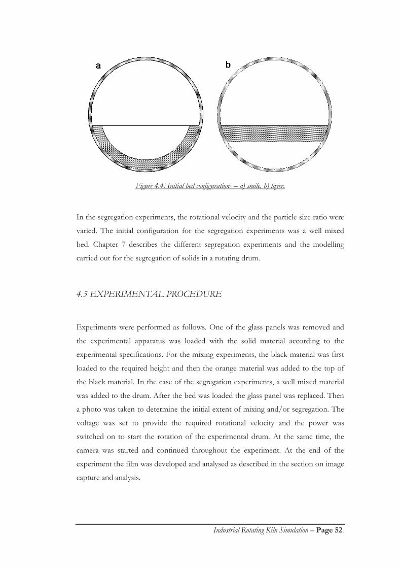
Industrial Rotating Kiln Simulation – Page 52.
Figure 4.4: Initial bed configurations – a) smile, b) layer.
In the segregation experiments, the rotational velocity and the particle size ratio were
varied. The initial configuration for the segregation experiments was a well mixed
bed. Chapter 7 describes the different segregation experiments and the modelling
carried out for the segregation of solids in a rotating drum.
4.5 EXPERIMENTAL PROCEDURE
Experiments were performed as follows. One of the glass panels was removed and
the experimental apparatus was loaded with the solid material according to the
experimental specifications. For the mixing experiments, the black material was first
loaded to the required height and then the orange material was added to the top of
the black material. In the case of the segregation experiments, a well mixed material
was added to the drum. After the bed was loaded the glass panel was replaced. Then
a photo was taken to determine the initial extent of mixing and/or segregation. The
voltage was set to provide the required rotational velocity and the power was
switched on to start the rotation of the experimental drum. At the same time, the
camera was started and continued throughout the experiment. At the end of the
experiment the film was developed and analysed as described in the section on image
capture and analysis.

Industrial Rotating Kiln Simulation – Page 53.
4.6 CHAPTER SUMMARY
In this chapter, the experimental materials and equipment have been described. A description of the
experimental rotating drum and the image capture equipment was given. The full experimental
method, from colouring of the raw shale to carrying out the experiments was also described. The
active layer, mixing and segregation experiments were briefly described and will be described in more
detail in the following chapters.

Industrial Rotating Kiln Simulation – Page 54.
CHAPTER 5
Active layer characterisation.
The literature review in Chapter 3 showed that mixing and segregation in a rolling
bed was caused by the granular flow in the active layer. Furthermore, the active layer
behaviour was shown to be dependent on the materials used in the experiments. This
chapter describes the work carried out to characterise the active layer in a rolling bed
as a function of drum diameter, particle diameter, rotational velocity and drum
loading. This characterisation will be used in the modelling of the mixing and/or
segregation of solids in the rotating drum operating in the rolling regime.
5.1 IMPORTANT ACTIVE LAYER PARAMETERS
ACTIVE LAYER FLOW
STAGNANT LAYER FLOW
CENTRE OF ROTATION[XO,YO]
Angle A-B ( AB)
APEX A[XA,YA]
APEX B[XB,YB]
Radius B (RB)
Radius A (RA)
Angle A ( A)
Distance A-B
Figure 5.1: Schematic of an ideal rolling bed.
The active layer is the zone of a rolling bed where the particles move relative to each
other resulting in mixing and/or segregation. In an idealised case of a rolling bed,
shown in Figure 5.1, the active layer is represented by a fraction of the bed height
along the exposed surface and the centre of rotation of the bed occurs at the mid
chord position. In a real system the active layer is not symmetrical and the rolling bed

Industrial Rotating Kiln Simulation – Page 55.
becomes wavelike as shown in Figure 5.2, which shows a skewed centre of rotation
of the bed. Both figures show the important parameters associated with the active
layer as described below.
STAGNANT LAYERFLOW
ACTIVE LAYER FLOW
APEX B[XB,YB]
CENTRE OF ROTATION[XO,YO]
APEX A[XA,YA]
Angle A-B ( AB)
Angle A ( A)
Radius B (RB)
Radius A (RA)
Distance A-B
Figure 5.2: Schematic of a real rolling bed illustrating the wave like upper surface shape.
The active layer – stagnant layer interface, indicated by the curved line separating the
active and stagnant layers, occurs where the material passed from the well packed
stagnant layer into the active layer or vice versa. The active layer flow shows the
direction of bulk material movement in the active layer, the stagnant layer flow
indicates the direction of bulk flow in the stagnant layer. As can be seen, the material
circulates around the centre of rotation of the bed and this centre can be considered
as a stationary point in the bed. Apex A and Apex B define the extremities of the
bed. These apexes are symmetrical about the centre of rotation for the ideal bed but
are asymmetrical in practical situations and thus distinguishing between these apexes
becomes important. The distance from Apex A to the centre of rotation of the bed is
termed Radius A and Radius B is the distance from Apex B to the centre of rotation.
Distance A-B is the distance between the two apexes. Angle A-B, AB, is the angle
between the two apexes and the horizontal axis. Angle A, A, is the angle between
the Distance A-B and Radius A. The measurement of these parameters was required

Industrial Rotating Kiln Simulation – Page 56.
for the segregation work. The active layer proportion, ALX , of the bed is the active
layer area of the bed divided by the total transverse bed area. Thus:
SLAL
ALAL
AAAX (5.1)
where AAL and ASL are the respective transverse areas of the active and the stagnant
layers.
5.2 EXPERIMENTAL PROCEDURE
Experiments were carried out to test the effect of drum loading, particle size, particle
type and rotational velocity on the above active layer parameters. Collecting the data
involved taking photographs of the rotating bed at a slow shutter speed. The motion
of the individual particles could be observed in the form of contour lines such as
shown in Figure 5.3. Active layer parameters were measured from these photographs.
The active and stagnant layers were cut out from photographs and the sections of the
photographs were weighed to obtain a relative size of both the active and stagnant
layers. In order to validate the weighing technique, 100 equal sized areas were cut
from photographic paper and weighed to ensure that the photographic paper used
was of uniform “density”. The photographic paper “density” was measured to be
2.4*10-4 g/mm² and the average error of this paper “density” was 1.2*10-6 g/mm²
which equals 0.5 % of the photographic paper “density”.
Another copy of the photograph was used to determine the location of the centre of
rotation of the bed and measure the distances from this centre of rotation to Apex A
and Apex B. The centre of rotation is the point around which the material circulates
shown by [X0,Y0] in Figure 5.3. The other geometric parameters, described above,
were also measured from this second copy of the photograph.

Industrial Rotating Kiln Simulation – Page 57.
Figure 5.3: Example of contour lines in the rolling bed.
Particle size ranges tested varied from 1.70 to 5.08 mm, the drum loading was altered
from 10 to 40 % of the drum volume, the rotational speed of the drum was in the
rolling regime, from 2 to 25 rpm and three different drum sizes of 570, 400 and 200
mm were tested. Different particle types, such as coloured shale and raw shale, were
also tested in the active layer experiments.
5.3 ACTIVE LAYER RESULTS FOR THE EXPERIMENTS IN
THE 570 mm DIAMETER DRUM
5.3.1 Active layer proportion
The active layer proportion was determined by weighing the active layer and stagnant
layer areas of the photographs taken in the active layer experiments. The active layer
proportion was calculated by substituting the area of the layers in Equation 5.1 with
the measured weights from the photographs. It was observed that particle size
differences and the use of raw shale instead of coloured shale did not affect the
active layer proportion of the bed.
[X0,Y0]
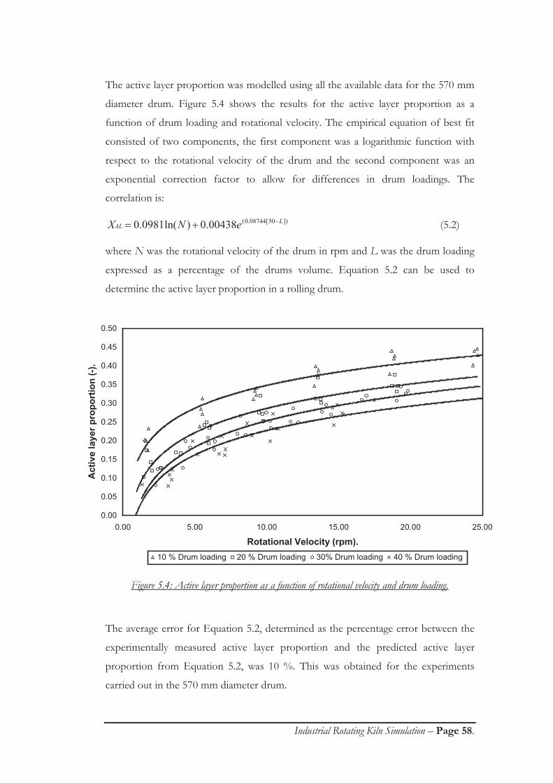
Industrial Rotating Kiln Simulation – Page 58.
The active layer proportion was modelled using all the available data for the 570 mm
diameter drum. Figure 5.4 shows the results for the active layer proportion as a
function of drum loading and rotational velocity. The empirical equation of best fit
consisted of two components, the first component was a logarithmic function with
respect to the rotational velocity of the drum and the second component was an
exponential correction factor to allow for differences in drum loadings. The
correlation is:
])50[08744.0(00438.0)ln(0981.0 LAL eNX (5.2)
where N was the rotational velocity of the drum in rpm and L was the drum loading
expressed as a percentage of the drums volume. Equation 5.2 can be used to
determine the active layer proportion in a rolling drum.
0.00
0.05
0.10
0.15
0.20
0.25
0.30
0.35
0.40
0.45
0.50
0.00 5.00 10.00 15.00 20.00 25.00
Rotational Velocity (rpm).
Act
ive
laye
r pro
port
ion
(-).
10 % Drum loading 20 % Drum loading 30% Drum loading 40 % Drum loading
Figure 5.4: Active layer proportion as a function of rotational velocity and drum loading.
The average error for Equation 5.2, determined as the percentage error between the
experimentally measured active layer proportion and the predicted active layer
proportion from Equation 5.2, was 10 %. This was obtained for the experiments
carried out in the 570 mm diameter drum.

Industrial Rotating Kiln Simulation – Page 59.
5.3.2 Mean velocity and flux of the stagnant layer
At the midchord of the bed, the stagnant layer has a linear velocity profile being zero
at the centre of rotation and equalling the drum speed at the drum wall (Nakagawa et
al, 1992; Boateng, 1993). This velocity profile is only valid if there is no slip between
the wall and the bed. Slip is avoided in the experiments since the drum wall was
roughened. Thus the mean velocity in the stagnant layer, SLV , is:
20R
dR
RdRVSL (5.3)
where is the rotational velocity in rad/s and R is the radius of the drum. Figure 5.5
illustrates the velocity profile in the transverse section of a rolling bed in a rotating
drum.
For the purpose of this work the flux is defined as the mean velocity of material in a
zone multiplied by the transverse area of that zone. The flux in the stagnant
layer, SL , is:
SLSLSL AV * (5.4)
where ASL is the area of the stagnant layer calculated from the Equation 5.2 and the
calculated transverse section area.

Industrial Rotating Kiln Simulation – Page 60.
Figure 5.5: Illustration of the transverse section velocity profile as measured by Nakagawa et al
(1992) & Boateng (1993).
5.3.3 Mean velocity and flux of the active layer
The mean velocity in the active layer of the bed was considered an important variable
in the modelling of both the mixing and segregation in the transverse section. Mass
conservation in the bed requires that the flux in the stagnant layer equals the flux in
the active layer. The flux in the active layer is:
SLALALAL AV * (5.5)
Thus the mean velocity in the active layer, ALV , is:
AL
AL
AL
SLSLAL
XXNR
AAVV 1
15 (5.6)
This correlation was used to calculate the mean active layer velocities in the mixing
and segregation experiments and shows the effect of drum size on the mean active
layer velocity.

Industrial Rotating Kiln Simulation – Page 61.
5.3.4 Radius A, Radius B and Angle A
The calculation of RA, RB and A are required for the segregation analysis since the
images for the segregation experiments were taken at a faster shutter speed than the
images for the active layer experiments, hence contour lines, such as those of Figure
5.3, were not observed.
Empirical correlations relating Radius A, Radius B and Angle A to the loading of the
drum and the rotational velocity of the bed were developed from the photographic
measurements. Multiple parameter linear regression was used in all cases. The
resulting correlations from the linear regression were:
LNRA 808.2211.282.168 (5.7)
LNRB 403.2606.461.193 (5.8)
LNA 126.0813.056.2 (5.9)
where RA is Radius A in mm, RB is Radius B in mm and A is Angle A in degrees.
Before the position of the centre of origin could be calculated, the gradient from
Apex A to Apex B needed to be calculated. This gradient was referred to as Angle A-
B, AB , in Figures 5.1 and 5.2. In the absence of the contour lines of Figure 5.3 the
location of the centre of rotation of the bed can be calculated as follows:
))sin(1(,))cos(1(],[ AABAAAABAAOO RYRXYX (5.10)
where [XO,YO] are the co-ordinates of the centre of rotation and [XA, YA] are the co-
ordinates of Apex A. Equations 5.7 to 5.10 are only applicable for the current
experimental setup using the 570 mm diameter drum.

Industrial Rotating Kiln Simulation – Page 62.
5.4 SCALABILITY OF ACTIVE LAYER RESULTS
Experiments were conducted to measure the active layer proportion in different
sized drums. Drum diameters of 400 and 200 mm were used. The experimental
active layer proportions at different rotational speeds and drum loadings were
compared to the active layer proportions calculated from Equation 5.2. The average
errors for the different experiments, as shown in Table 5.1, were within the
experimental error hence it can be assumed that Equation 5.2 could be applied to
determine the active layer proportion for different sized drums.
Loading 200 mm 400 mm10% 10.7 6.920% 3.4 2.630% 3.0 1.440% 2.1 4.0
Drum Diameter
Table 5.1: Deviation, as a percentage, between the experimental results and the predicted results using
Equation 5.2 for the active layer proportion in the 200 and 400 mm diameter drums.
From this active layer proportion the mean velocity of the particles in the active layer
in any sized drum can be calculated using Equation 5.6. This active layer velocity will
be used in the modelling as a scaling parameter in line with the observations of
Williams & Khan (1973) who found that suitable scaling parameters needed to
represent the movement of particles. The literature showed that the active layer is
responsible for mixing and segregation in a rotating kiln. Thus the active layer should
be included as a modelling parameter for the modelling of mixing or segregation in a
rotating drum. By incorporating the active layer properties the derived model can
then be applied to predict the behaviour in different sized rotating drums by
calculating the active layer velocity of the different sized drum, such as industrial
rotating kiln.

Industrial Rotating Kiln Simulation – Page 63.
5.5 CHAPTER SUMMARY
In this chapter the active layer has been characterised. A correlation was derived to predict the active
layer proportion and the mean velocity of particles in the active layer. This correlation was dependent
on the rotational velocity and the drum loading. The geometry of the active layer was also studied to
allow the centre of rotation of the bed to be determined and will be used in a later chapter to develop
a solid segregation model. The chapter was concluded with the derivation of suitable scaling
parameters to allow the mixing and/or segregation of an industrial rotating kiln to be determined
based on experiments carried out in laboratory sized equipment.

Industrial Rotating Kiln Simulation – Page 64.
CHAPTER 6
Mixing in the transverse direction of a rotary drum.
The mixing mechanisms of granular materials were described in Chapter 2. Previous
studies revealed that there is a lack of quantifying models to predict both the mixing
rate and the final amount of mixing in the transverse direction of rotating drums. In
this chapter models will be developed to predict, as a quantitative measure, the
mixing rates and the final amounts of mixing so that the mixing of solids in rotating
kilns can be predicted.
Before these models could be developed, new experimental methodologies were
required. These new experimental methods used image analysis programming to
determine the extent of mixing and will also be described in this chapter.
6.1 TRANSVERSE MIXING EXPERIMENTS
The mixing behaviour of solids in the transverse section of a rotating drum was
investigated in the mixing experiments. The experimental variables tested were the
rotational velocity, the percentage drum loading, the particle size and the material
ratio. The rotational velocity, N, ranged from 5 to 19 rpm covering the rolling
regime. Drum loadings, L, of 6 to 40% of the total drum volume were used. The
particle size range, dp, was varied from 0.89 to 5.08 mm. Experimental material ratios
of the black to orange material were altered from 0.55 to 2.70. The material ratio was
set equal to the experimentally measured material ratio unless the experimentally
measured material ratio was less than one, in which case the material ratio equalled
the inverse of the experimental material ratio.
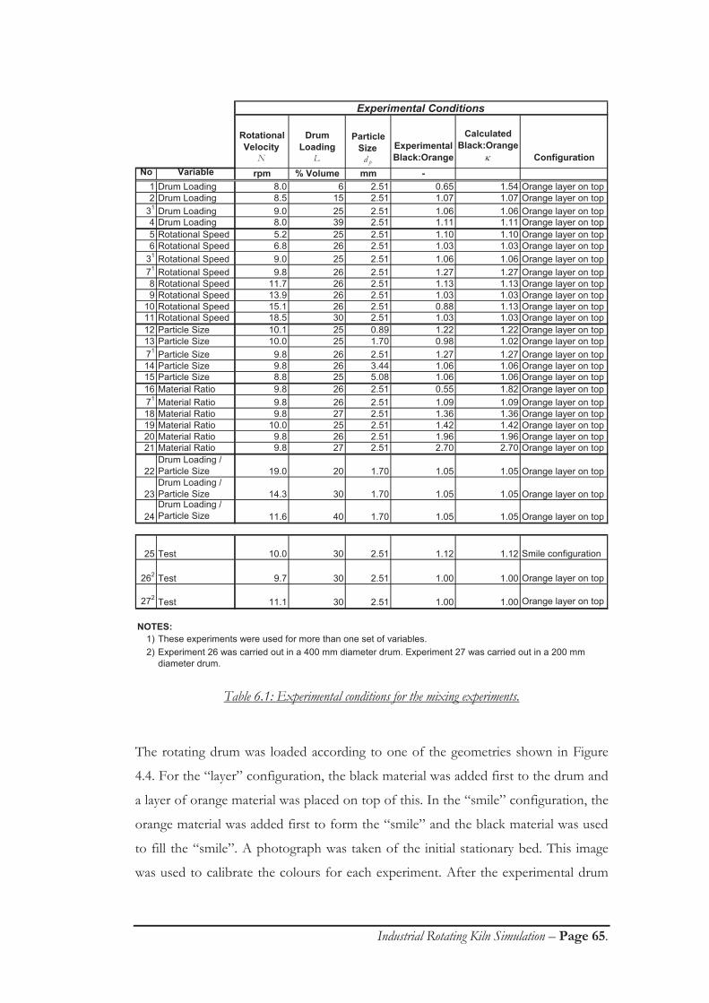
Industrial Rotating Kiln Simulation – Page 65.
Rotational Velocity
N
Drum Loading
L
Particle Size
d p
Experimental Black:Orange
Calculated Black:Orange
ConfigurationNo Variable rpm % Volume mm -
1 Drum Loading 8.0 6 2.51 0.65 1.54 Orange layer on top2 Drum Loading 8.5 15 2.51 1.07 1.07 Orange layer on top
31 Drum Loading 9.0 25 2.51 1.06 1.06 Orange layer on top4 Drum Loading 8.0 39 2.51 1.11 1.11 Orange layer on top5 Rotational Speed 5.2 25 2.51 1.10 1.10 Orange layer on top6 Rotational Speed 6.8 26 2.51 1.03 1.03 Orange layer on top
31 Rotational Speed 9.0 25 2.51 1.06 1.06 Orange layer on top71 Rotational Speed 9.8 26 2.51 1.27 1.27 Orange layer on top8 Rotational Speed 11.7 26 2.51 1.13 1.13 Orange layer on top9 Rotational Speed 13.9 26 2.51 1.03 1.03 Orange layer on top
10 Rotational Speed 15.1 26 2.51 0.88 1.13 Orange layer on top11 Rotational Speed 18.5 30 2.51 1.03 1.03 Orange layer on top12 Particle Size 10.1 25 0.89 1.22 1.22 Orange layer on top13 Particle Size 10.0 25 1.70 0.98 1.02 Orange layer on top71 Particle Size 9.8 26 2.51 1.27 1.27 Orange layer on top14 Particle Size 9.8 26 3.44 1.06 1.06 Orange layer on top15 Particle Size 8.8 25 5.08 1.06 1.06 Orange layer on top16 Material Ratio 9.8 26 2.51 0.55 1.82 Orange layer on top71 Material Ratio 9.8 26 2.51 1.09 1.09 Orange layer on top18 Material Ratio 9.8 27 2.51 1.36 1.36 Orange layer on top19 Material Ratio 10.0 25 2.51 1.42 1.42 Orange layer on top20 Material Ratio 9.8 26 2.51 1.96 1.96 Orange layer on top21 Material Ratio 9.8 27 2.51 2.70 2.70 Orange layer on top
22Drum Loading / Particle Size 19.0 20 1.70 1.05 1.05 Orange layer on top
23Drum Loading / Particle Size 14.3 30 1.70 1.05 1.05 Orange layer on top
24Drum Loading / Particle Size 11.6 40 1.70 1.05 1.05 Orange layer on top
25 Test 10.0 30 2.51 1.12 1.12 Smile configuration
262 Test 9.7 30 2.51 1.00 1.00 Orange layer on top
272 Test 11.1 30 2.51 1.00 1.00 Orange layer on top
NOTES:1)2)
These experiments were used for more than one set of variables.Experiment 26 was carried out in a 400 mm diameter drum. Experiment 27 was carried out in a 200 mm diameter drum.
Experimental Conditions
Table 6.1: Experimental conditions for the mixing experiments.
The rotating drum was loaded according to one of the geometries shown in Figure
4.4. For the “layer” configuration, the black material was added first to the drum and
a layer of orange material was placed on top of this. In the “smile” configuration, the
orange material was added first to form the “smile” and the black material was used
to fill the “smile”. A photograph was taken of the initial stationary bed. This image
was used to calibrate the colours for each experiment. After the experimental drum

Industrial Rotating Kiln Simulation – Page 66.
was closed, the rotation was started and the camera was set on automatic. An image
of the moving bed was taken every 0.26 seconds until the end of the film. This film
was then processed and scanned into a personal computer using the equipment
described in Chapter 4. The images were analysed to obtain a measure of the contact
distance between the two materials, as described below. In all cases complete mixing
was achieved within 1 minute.
In this work a quantitative measure of mixing was sought. Hence the contact
distance was established. This contact distance represents the one dimensional
circumferential contact between the two different materials. Previous work, such as
Woodle & Munro (1991), only expressed the mixing qualitatively. In the current
work it is desired to simulate an industrial process where heat transfer between
different materials is important and hence the use of a quantitative parameter, such
as the contact distance, is beneficial since heat transfer between materials is
dependent on the amount of contact between those materials.
6.2 EXPERIMENTAL ANALYSIS METHODOLOGY
After the images were scanned into a computer as bitmaps, they were analysed using
image analysis software specifically written for this task. Bitmaps are described in
Appendix 1 and the pseudo-codes for the image analysis software are included in
Appendix 2. The first step of the image analysis involved converting the bitmap file
of the image into an array of data. This numerical array represented the colour
specifications of each pixel in the image. The colour of each pixel indicated what type
of particle was represented by that pixel. Three different colour specifications were
considered in the mixing work, these being the black colour type for the black
particles, the orange colour type for the orange particles and the white colour type
for the background of the drum. The colour specifications were determined from
experimental images to ensure that the colour specifications matched the colours of
the materials used.

Industrial Rotating Kiln Simulation – Page 67.
Contact between the two materials occurred if adjacent pixels represented different
colour types. The total contact distance could be calculated for either the black or the
orange colour specification but the orange colour specification was chosen. Since the
contact distance between the orange and the black material was required it did not
matter which colour was chosen as the basis. The total contact distance was
quantified by calibrating the physical size represented by a pixel in the image. Contact
between orange and white pixels was not considered since this did not physically
represent mixing of the two materials. White-orange contact signified the presence of
an orange particle next to a boundary of the drum and hence provided no contact
information.
The mixing image analysis methodology may be best illustrated by means of an
example. Figure 6.1 shows an enlarged extract from an image of a well mixed bed. A
grid was superimposed to represent the different pixels of a bitmap. P[i,j] represent
the pixel in the ith row and the jth column of Figure 6.1. Black pixels were defined as
B, white pixels were defined as W and the orange pixels were defined by a numerical
value from 0 to 4 on a freckled background. This number indicated the number of
contact occurrences between that orange pixel and surrounding black pixels as
described below.
The contact distance between the orange and the black particles was calculated using
the orange material as a basis. Only contacts between adjacent edges were
considered. Adjacent corners of different coloured pixels would only indicate that
there was a point of contact and not a distance of contact. Points of contact were not
included in the determination of the contact distance between the different coloured
materials in the image. Edge to edge contact increased the contact of that image by 1.
For example looking at the pixel in column 1 and row 1 of Figure 6.1, P[1,1], which
was an orange pixel, the contact between the surrounding pixels and the current pixel
was 1 since the only contact with black material was due to P[1,2]. The contact from
P[1,2] was not calculated since this was not of the orange type. Moving along to
P[2,2], which was another orange pixel, the contact of this pixel was 2 because of
P[1,2] and P[3,2] both of which were black. Note that P[2,2] had 2 edge contacts,
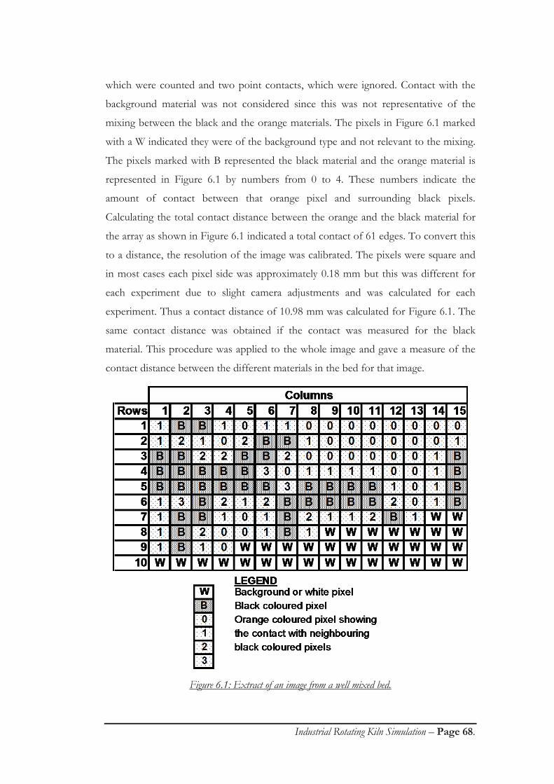
Industrial Rotating Kiln Simulation – Page 68.
which were counted and two point contacts, which were ignored. Contact with the
background material was not considered since this was not representative of the
mixing between the black and the orange materials. The pixels in Figure 6.1 marked
with a W indicated they were of the background type and not relevant to the mixing.
The pixels marked with B represented the black material and the orange material is
represented in Figure 6.1 by numbers from 0 to 4. These numbers indicate the
amount of contact between that orange pixel and surrounding black pixels.
Calculating the total contact distance between the orange and the black material for
the array as shown in Figure 6.1 indicated a total contact of 61 edges. To convert this
to a distance, the resolution of the image was calibrated. The pixels were square and
in most cases each pixel side was approximately 0.18 mm but this was different for
each experiment due to slight camera adjustments and was calculated for each
experiment. Thus a contact distance of 10.98 mm was calculated for Figure 6.1. The
same contact distance was obtained if the contact was measured for the black
material. This procedure was applied to the whole image and gave a measure of the
contact distance between the different materials in the bed for that image.
Figure 6.1: Extract of an image from a well mixed bed.
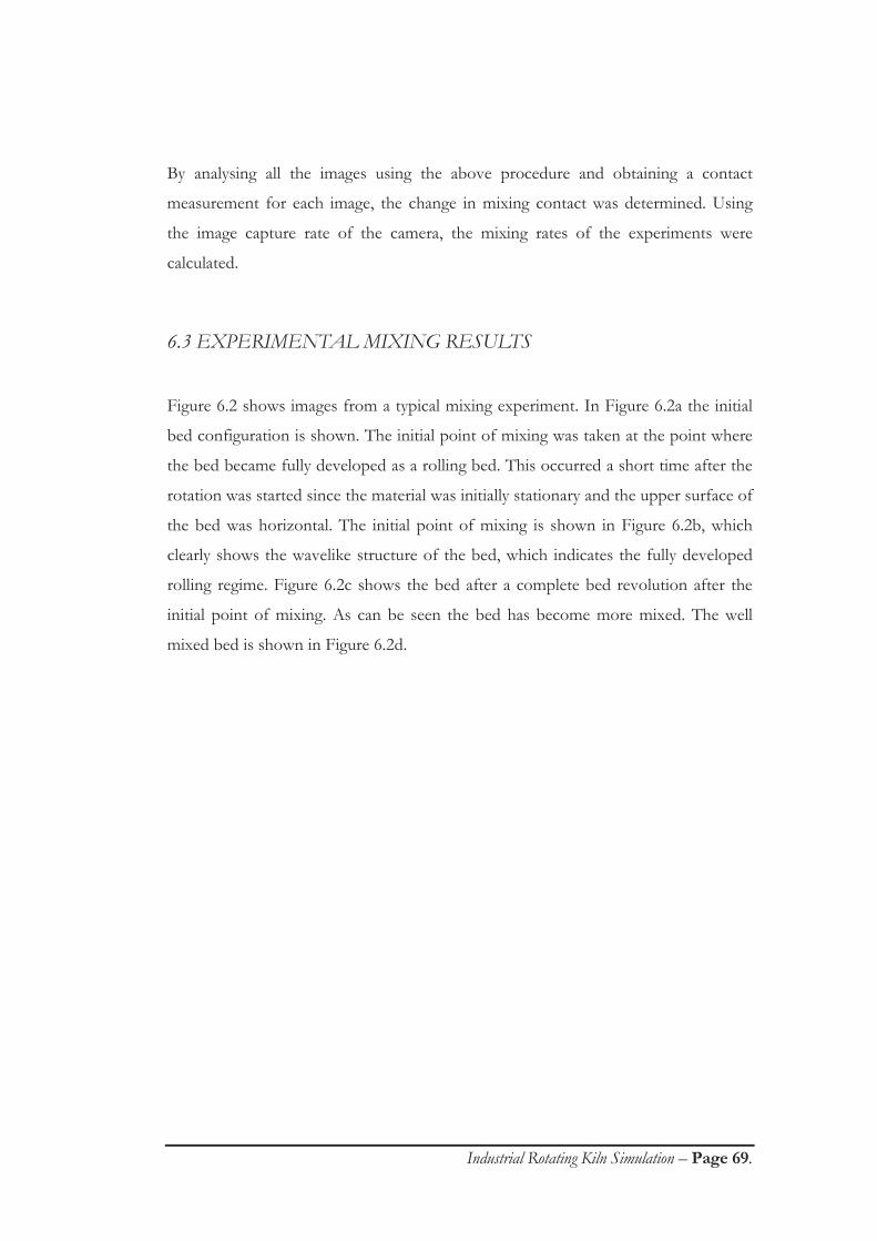
Industrial Rotating Kiln Simulation – Page 69.
By analysing all the images using the above procedure and obtaining a contact
measurement for each image, the change in mixing contact was determined. Using
the image capture rate of the camera, the mixing rates of the experiments were
calculated.
6.3 EXPERIMENTAL MIXING RESULTS
Figure 6.2 shows images from a typical mixing experiment. In Figure 6.2a the initial
bed configuration is shown. The initial point of mixing was taken at the point where
the bed became fully developed as a rolling bed. This occurred a short time after the
rotation was started since the material was initially stationary and the upper surface of
the bed was horizontal. The initial point of mixing is shown in Figure 6.2b, which
clearly shows the wavelike structure of the bed, which indicates the fully developed
rolling regime. Figure 6.2c shows the bed after a complete bed revolution after the
initial point of mixing. As can be seen the bed has become more mixed. The well
mixed bed is shown in Figure 6.2d.

Industrial Rotating Kiln Simulation – Page 70.
a) initial bed configuration, this image was used to calibrate the colours of the materials, b) initial point taken for the calculation of the mixing rate showing the development of the rolling regime, c) image one complete bed revolution after the initial mixing point showing the widening of the orange
material and d) fully mixed bed configuration. Figure 6.2: Sample photos from a typical mixing experiment.
Figure 6.3 shows the results from a typical mixing experiment. The plot shows the
contact distance for a series of images plotted against the experimental time. Both
the mixing rate and the final contact distance were calculated for each experiment.
The results showed that the mixing occurred at a constant rate. Small fluctuations
were observed about the final contact distance. The experimental error of the mixing
rate and the final contact distance were also calculated.
a) b)
d) c)

Industrial Rotating Kiln Simulation – Page 71.
0
5000
10000
15000
20000
25000
30000
35000
40000
45000
0 10 20 30 40 50 60
Time (s)
Con
tact
dis
tanc
e (m
m)
MIXING DYNAMICSContact Distance = 1656 * Time + 6012 mmExperimental Mixing Rate Error = 141 mm/s
STEADY STATEFinal Contact Distance = 41246 mm
Experimental Final Contact Distance Error = 719 mm
l 0
l f
t ft 0
Figure 6.3: Typical results for a mixing experiment, this graph shows the results for experiment 3.
The mixing rate, , was calculated over the linear “mixing dynamics” section of
Figure 6.3. The resulting equation was of the following type:
0
0
ttll
f
f (6.1)
where lf was the final contact distance and l0 was the initial contact distance, in mm,
between the orange and black materials obtained from images similar to Figure 6.2b.
tf was the time when the final contact distance was first reached and t0 was the time
corresponding to the initial contact distance, taken as 0.
Table 6.2 contains the experimental mixing rates and the experimental mixing rate
errors as well as the calculated data for the mixing experiments that were used in the
modelling of the mixing rate. The experimental mixing rate error was calculated by
averaging the relative errors between the overall experimental mixing rate and the
mixing rate calculated for the individual data points.

Industrial Rotating Kiln Simulation – Page 72.
Experimental Mixing Rate
Experimental Mixing Rate
ErrorActive layer Percentage
Active layer velocity
(vAL)
Active Layer Parameter
Predicted Mixing Rate From Model
Predicted Mixing Rate
DeviationNo Variable mm/s % mm/s mm³/s mm/s %
1 Drum Loading 975 22 41 348 328741 494 492 Drum Loading 1326 11 30 576 849801 1277 4
31 Drum Loading 1656 9 25 792 1397108 2099 274 Drum Loading 1897 16 22 870 1733693 2605 375 Rotational Speed 1296 11 20 623 962611 1446 126 Rotational Speed 1984 17 22 703 1193040 1793 10
31 Rotational Speed 1656 9 25 792 1397108 2099 2771 Rotational Speed 2441 9 26 836 1419802 2133 138 Rotational Speed 2440 9 28 911 1666058 2503 39 Rotational Speed 2409 12 29 995 1935432 2908 21
10 Rotational Speed 3235 9 30 1045 2004546 3012 711 Rotational Speed 3290 7 31 1219 2622433 3940 2012 Particle Size 3167 15 27 836 1994858 2997 513 Particle Size 2665 16 26 830 1805696 2713 271 Particle Size 2441 9 26 836 1419802 2133 1314 Particle Size 1496 9 26 830 1160047 1743 1715 Particle Size 947 19 25 783 519060 780 1816 Material Ratio 1654 17 26 838 1180029 1773 771 Material Ratio 2441 9 26 836 1503368 2259 718 Material Ratio 2010 11 26 842 1398547 2101 519 Material Ratio 1845 10 26 830 1330790 2000 820 Material Ratio 1502 13 26 841 1119301 1682 1221 Material Ratio 1271 16 26 842 783465 1177 7
22Drum Loading / Particle Size 3604 16 35 1068 2350170 3531 2
23Drum Loading / Particle Size 5183 11 28 1072 2619874 3937 24
24Drum Loading / Particle Size 3429 9 25 1035 2737878 4114 20
Minimum 7 Minimum 2Maximum 22 Maximum 49Average 12 Average 14
25 Test 2113 9 25 893 1674010 2515 19
262 Test 1217 8 25 615 835875 1256 3
272 Test 356 23 26 328 228779 344 3
NOTES:1)2)
Experimental Variables Calculated and Modelling Variables
These experiments were used for more than one set of variables.Experiment 26 was carried out in a 400 mm diameter drum. Experiment 27 was carried out in a 200 mm diameter drum.
ALV
Table 6.2: Experimental mixing rates and calculated data for the modelling of the mixing rates.
The final contact distance, lf, of an experiment was taken as the average of the steady
state contact distances of the mixing experiment. The experimental error of the
steady states was calculated as the average error from this steady state value. Table
6.3 contains the experimental final contact distance and the experimental final
contact distance error. The calculated data, used in the modelling of the final contact
distance is also shown in Table 6.3 and is described below.

Industrial Rotating Kiln Simulation – Page 73.
Experimental Final Contact
Distance l f
Experimental Final Contact
Distance Error
Final Contact Distance
Parameter
Predicted Final Contact
Distance from Model
Final Contact Distance Deviation
No Variable mm % mm³ mm %1 Drum Loading 13022 4 164049 8661 332 Drum Loading 23457 3 476973 25182 7
31 Drum Loading 41246 2 815327 43046 44 Drum Loading 64813 3 1236529 65284 15 Rotational Speed 42027 3 809213 42723 26 Rotational Speed 43844 4 851471 44954 3
31 Rotational Speed 41246 2 815327 43046 471 Rotational Speed 47524 2 775979 40969 148 Rotational Speed 44456 2 814924 43025 39 Rotational Speed 40254 3 851174 44939 12
10 Rotational Speed 43229 2 826417 43632 111 Rotational Speed 44869 3 982466 51870 1612 Particle Size 65394 6 1031337 54450 1713 Particle Size 54137 3 970601 51244 571 Particle Size 47524 2 775979 40969 1414 Particle Size 31526 2 666085 35167 1215 Particle Size 24705 4 369404 19503 2116 Material Ratio 24765 10 615593 32501 3171 Material Ratio 47524 2 833473 44004 718 Material Ratio 44320 2 766944 40492 919 Material Ratio 38388 2 707349 37345 320 Material Ratio 30266 4 570588 30125 021 Material Ratio 21311 7 338376 17865 16
22Drum Loading / Particle Size 40047 7 761407 40199 0
23Drum Loading / Particle Size 60785 4 1142110 60299 1
24Drum Loading / Particle Size 71198 4 1522814 80398 13
Minimum 2 Minimum 0Maximum 10 Maximum 33Average 4 Average 10
25 Test 37500 2 948945 50101 34
262 Test 22148 2 488575 25795 16
272 Test 5399 5 122144 6449 19
NOTES:1)2)
Experimental Variables Calculated and Modelling Variables
These experiments were used for more than one set of variables.Experiment 26 was carried out in a 400 mm diameter drum. Experiment 27 was carried out in a 200 mm diameter drum.
Table 6.3: Experimental final contact distances and calculated data for the modelling of the final
contact distances.

Industrial Rotating Kiln Simulation – Page 74.
6.4 ANALYSIS OF THE EXPERIMENTAL MIXING RESULTS
As described in Chapter 3, the transverse section of a rolling bed consists of both an
active and a stagnant layer. The active layer is responsible for all the mixing in a
rotating drum (Boateng, 1993).
6.4.1 Stepwise mixing behaviour
The first 10 seconds of mixing from Figure 6.3 are redrawn in Figure 6.4. Enlarging
the experimental results in this manner showed that the mixing occurred through a
series of steps. For experiment 3 these steps were approximately 2 seconds in length
and this time equalled the calculated time that the material spent in the stagnant layer
during one bed revolution in experiment 3. The time spent in the stagnant layer was
calculated from the geometry of the rotating drum, the bed loading and the rotational
velocity. An increase in the contact distance occurred when the two different
materials entered the active layer together and subsequently mixed. The time spent in
the active layer was much shorter when compared to the stagnant layer due to the
mass flux conservation of the active and stagnant layers as described in Chapter 5.
The magnitude of the steps were approximately constant showing that the mixing
rate was indeed constant. As time progressed, the two materials become more mixed
and the distinction between the steps was reduced until the steps were not observed
at the steady state, ie when all material entering the active layer was well mixed. This
stepwise behaviour was sufficient proof to show that the mixing only occurred in the
active layer of the bed of solids in a rotating drum and validates the use of the active
layer in subsequent modelling.
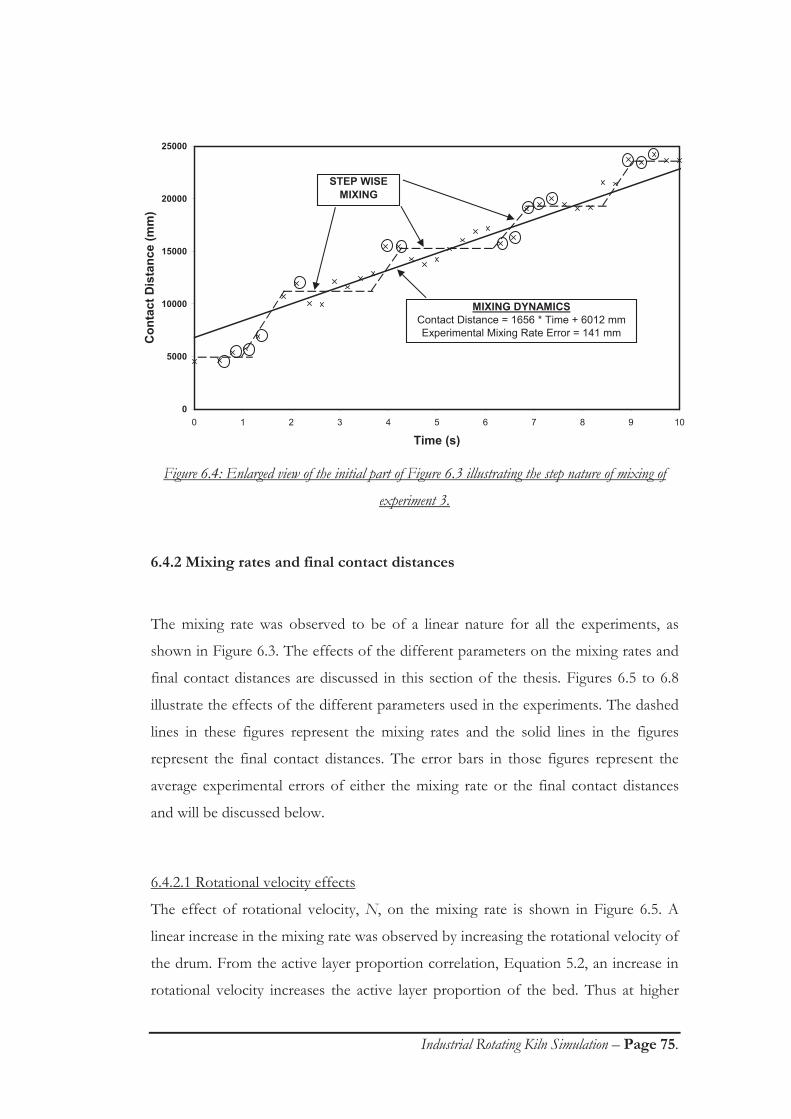
Industrial Rotating Kiln Simulation – Page 75.
0
5000
10000
15000
20000
25000
0 1 2 3 4 5 6 7 8 9 10
Time (s)
Con
tact
Dis
tanc
e (m
m)
STEP WISE MIXING
MIXING DYNAMICSContact Distance = 1656 * Time + 6012 mmExperimental Mixing Rate Error = 141 mm
Figure 6.4: Enlarged view of the initial part of Figure 6.3 illustrating the step nature of mixing of
experiment 3.
6.4.2 Mixing rates and final contact distances
The mixing rate was observed to be of a linear nature for all the experiments, as
shown in Figure 6.3. The effects of the different parameters on the mixing rates and
final contact distances are discussed in this section of the thesis. Figures 6.5 to 6.8
illustrate the effects of the different parameters used in the experiments. The dashed
lines in these figures represent the mixing rates and the solid lines in the figures
represent the final contact distances. The error bars in those figures represent the
average experimental errors of either the mixing rate or the final contact distances
and will be discussed below.
6.4.2.1 Rotational velocity effects
The effect of rotational velocity, N, on the mixing rate is shown in Figure 6.5. A
linear increase in the mixing rate was observed by increasing the rotational velocity of
the drum. From the active layer proportion correlation, Equation 5.2, an increase in
rotational velocity increases the active layer proportion of the bed. Thus at higher

Industrial Rotating Kiln Simulation – Page 76.
rotational velocities there was more material in the active layer and from the mean
active layer velocity correlation, Equation 5.6, this material travels faster within the
active layer. This is shown in the active layer velocity column of Table 6.2. This
indicated that at the higher rotational velocities there was more material in the active
layer and a higher driving force to mix due to the increased velocity. This leads to
faster mixing rates at higher rotational velocities as observed in the rotating drum.
For the rotational velocity experiments, all the experiments obtained similar final
contact distances, as indicated by the horizontal solid line of Figure 6.5. This was
expected since similar initial bed configurations were used for each of the rotational
velocity experiments. The small differences in the final contact distances were due to
the small differences in the initial configurations of the experiments.
0
500
1000
1500
2000
2500
3000
3500
4000
0 2 4 6 8 10 12 14 16 18 20
Rotational Velocity - N (rpm)
Mix
ing
Rat
e -
(mm
/s)
0
10000
20000
30000
40000
50000
60000
Fina
l Con
tact
Dis
tanc
e - l
f (m
m)
Mixing Rate
Steady State Contact
Figure 6.5: Measured mixing rates ( ) and final contact distances (lf) with respect to the rotational
velocity (N) of the drum.
6.4.2.2 Drum loading effects
Figure 6.6 shows the mixing results for the drum loading experiments. The mixing
rate increased linearly as the drum loading, L, increased. This can once again be
attributed to the active layer. As the drum loading increases, the active layer
proportion of the bed decreased but the actual size of the active layer and the mean

Industrial Rotating Kiln Simulation – Page 77.
active layer velocity increased. This results in an increased mixing rate as the loading
was increased. A linear dependence was observed between the final contact distance
and the drum loading in the loading experiments. This was expected since in the
presence of more material, a larger amount of contact can be obtained between the
materials.
0
500
1000
1500
2000
2500
0% 5% 10% 15% 20% 25% 30% 35% 40% 45%
Drum Loading - L (%)
Mix
ing
Rat
e -
(mm
/s)
0
10000
20000
30000
40000
50000
60000
70000
Fina
l Con
tact
Dis
tanc
e - l
f (m
m)
Mixing Rate
Steady State Contact
Figure 6.6: Measured mixing rates ( ) and final contact distances (lf) with respect to drum loading
(L) by percentage volume.
6.4.2.3 Particle size effects
The particle size, dp, effect is shown in Figure 6.7. This figure shows a linear increase
in mixing rate by decreasing the particle size. Since the drum loading and rotational
speeds were constant throughout the particle size experiments, the active layer
proportion and active layer velocities were also constant and cannot explain the
current behaviour. However, a certain volume of smaller particles has a larger surface
area compared to an equal sized volume of larger particles. Thus the total possible
contact distance in a fixed size active layer would increase with decreasing particle
size. This was reflected by the increase in mixing rate for the smaller particles. A
higher final contact distance was obtained for smaller particles. A linear dependence
was observed between the final contact distance and the particle size.

Industrial Rotating Kiln Simulation – Page 78.
0
500
1000
1500
2000
2500
3000
3500
4000
0.00 1.00 2.00 3.00 4.00 5.00 6.00
Particle Size - d p (mm)
Mix
ing
Rat
e -
(mm
/s)
0
10000
20000
30000
40000
50000
60000
70000
80000
Fina
l Con
tact
Dis
tanc
e - l
f (m
m)
Mixing Rate
Steady State Contact
Figure 6.7: Measured mixing rates ( ) and final contact distances (lf) as a function of particle size
(dp).
6.4.2.4 Material ratio effects
The results obtained from varying the proportion of the black to orange material in
the drum are shown in Figure 6.8. The mixing rate varies linearly over the material
ratio range tested. This trend cannot be explained using the active layer properties
since the rotational velocity and drum loading were similar for the material ratio
experiments resulting in equal mean active layer velocities. As the calculated material
ratio increased the mixing rate decreased. This can be explained by considering the
total contact distance possible for each of the materials. As the material ratio
increased there was an excess of one type of material and a shortfall for the other
type of material in the bed, which resulted in a quicker mixing of the lesser material.
However if this material entered the active layer uniformly, the tendency to mix in
each bed revolution decreased since there was less material to mix. Increasing the
ratio of the materials resulted in a linear reduction of the final contact distance in the
bed. A maximum final contact distance would be obtained for a material ratio of 1.
In this case the total perimeters for the orange or the black material equalled. If the
ratio is increased, the perimeter of one material increases but the total perimeter of

Industrial Rotating Kiln Simulation – Page 79.
the other material decreases. Since contact only occurred between the two different
materials, a decrease in the total perimeter of one material would result in a lower
final contact distance and this is reflected by the results of Figure 6.8.
0
500
1000
1500
2000
2500
3000
1.00 1.20 1.40 1.60 1.80 2.00 2.20 2.40 2.60 2.80
Material Ratio - (-)
Mix
ing
Rat
e -
(mm
/s)
0
5000
10000
15000
20000
25000
30000
35000
40000
45000
50000
Fina
l Con
tact
Dis
tanc
e - l
f (m
m)
Mixing Rate
Steady State Contact
Figure 6.8: Measured mixing rates ( ) and final contact distances (lf) with respect to calculated
material ratios ( ).
6.4.3 Analysis of the experimental errors
The experimental errors for the final contact distance were used as a measure of the
indeterminate experimental error of the experiments. This experimental error
included fluctuations in the material count. These fluctuations arose due to the seal
between the two panes of glass or the clamps holding the glass face to the drum,
both of which caused some material and thus contact distance to be hidden at certain
times during the experiments.
Incorrect film exposure was another source of experimental error. However,
checking the ratios of the colours in each image eliminated this. If the image was not
exposed correctly the ratios of the black to orange pixels would differ significantly

Industrial Rotating Kiln Simulation – Page 80.
compared to other images from the same experiment. In that case the image was
discarded and not used in the image analysis.
The average relative experimental error for the final contact distance for all the
experiments was 4%. The average relative experimental error for the mixing rate for
all the experiments was 12%. The maximum errors were 10% and 22% for the
experimental final contact distances and the experimental mixing rates respectively.
The experimental errors described for the final contact distances were also applicable
to the mixing rate data. One further aspect of the mixing rate experimental error to
be considered was due to the step nature of mixing. This behaviour forced data away
from the constant rate line and is illustrated the circled data points of Figure 6.4. This
stepwise mixing behaviour caused the experimental mixing rate errors to be larger
than the experimental final contact distance errors.
6.5 MODELLING OF THE MIXING IN THE TRANSVERSE
DIRECTION OF A ROLLING DRUM
In this section of the thesis, the experimental mixing results are analysed and
modelled so that they can be used to predict the mixing rates and the final amount of
mixing in a rolling drum as a quantitative measure. Suitable scaling criteria need to be
included in the model so that it can be used to predict the mixing in different sized
drums.
6.5.1 Mixing rate modelling
The experimental results showed that the mixing rate was linearly dependent on the
drum’s rotational velocity, the loading of the drum, the mean particle size and the
material ratio. Thus the mixing rate can be expressed as:
),,,(1 pdLNf (6.2)

Industrial Rotating Kiln Simulation – Page 81.
However to develop a mixing rate model which can be applied to any drum the
scaling factors need to be included in this mixing rate model. The results from
Chapter 5 and the stepwise behaviour of the mixing rate show that the mixing occurs
in the active layer. Since the rotational velocity and the drum loading affect the solid
behaviour in the active layer these parameters will be replaced by active layer
properties as part of the model development. The mean active layer velocity is used
as one of these parameters as this velocity is a measure of how fast the material is
traveling in the active layer, which affects the mixing rate. The size of the active layer
is also important and will be the second active layer parameter. Therefore Equation
6.2 can be rewritten as follows:
),,,(2 pALAL dAVf (6.3)
The particle size and material ratio effects are shown in Figure 6.7 and Figure 6.8
respectively. It was observed that increasing the particle size or the material ratio
resulted in a linear decrease in the mixing rate. In the modelling of the mixing rate, it
was assumed that the mixing rate could not become negative and this in turn placed
restrictions on the particle size and the material ratio that could be used in the model.
Thus the overall effect of the particle size with respect to the mixing rate was:
)( ,3 pMAXp ddf (6.4)
where dp,MAX is the limiting particle size, beyond which the mixing rate was assumed
to be zero.
A similar correlation was derived for the material ratio effect:
)(4 MAXf (6.5)
where MAX is the limiting material ratio, beyond which the mixing rate was assumed
to be zero.
Equation 5.6 showed that the mean active layer velocity is a function of the
rotational velocity of the drum, and to a lesser extent the loading of the drum. This
indicates that the mixing rate should respond to changes in the active layer velocity
Industrial Rotating Kiln Simulation – Page 82.
similarly as it would respond to changes in the rotational velocity of the drum.
Equation 6.6 shows this relationship:
)(5 ALVf (6.6)
Finally, changes in the drum loading resulted in changing the area of the bed.
However the mixing only occurred in the active layer and thus the transverse area of
the active layer was required, shown in Equation 6.7:
)(6 ALAf (6.7)
From the experimental results linear relationships were observed in many cases, thus
f3, f4 and f5 were linear in nature. However the behaviour of the active layer area was
not easily determined as it was dependent on the rotational velocity, the drum
loading and the size of the drum. A range of functions were tested and it was found
that the mixing rate varied linearly with the square root of the active layer area. An
active layer parameter, , was developed to combine all the parameters that had an
effect on the mixing rate and is shown in Equation 6.8:
)).(.(. , MpMpALAL ddAV (6.8)
The active layer parameter was calculated for all experiments and the mixing rate was
correlated using this active layer parameter. Figure 6.9 shows that a linear relationship
exists between the active layer parameter and the mixing rate. This linear relationship
passes through zero, which makes it physically realistic. For example, if the bed was
stationary, ALV and ALA would both be zero and hence the mixing rate should also
be zero. The mixing rate was calculated as follows:
= 1.503*10-3 (6.9)
The confirmation data points in Figure 6.9 indicate the experimentally measured
mixing rates for experiments 25 to 27 and will be discussed below.

Industrial Rotating Kiln Simulation – Page 83.
= 1.503*10-3 mm/s
0
1000
2000
3000
4000
5000
6000
0 500000 1000000 1500000 2000000 2500000 3000000
Active Layer Parameter - (mm³/s)
Mix
ing
Rat
e -
(mm
/s)
Experimental Data Points and Error Bars
Confirmation Data Points
Figure 6.9: Modelling of the mixing rate ( ) as a function of the active layer parameter ( ).
The deviations between the predictions from the mixing rate model and the
experimental mixing rate results were calculated as a percentage difference between
the predicted mixing rate and the experimental mixing rate. The average deviation
was 14% and the maximum deviation was 49%. The largest deviation occurred at the
lowest value of the active layer parameter.
6.5.2 Final mixing contact distance modelling
The important parameters for determining the final contact value of solids in a
rotating drum were the drum loading, the particle size and the material ratio. It was
observed that all these parameters linearly affected the final contact value. Once
again, for scaling purposes, the drum loading was replaced by the transverse area of
the bed. The rotational velocity did not affect the final mixing contact distance. The
final contact distance parameter, in mm³, correlation is shown in Equation 6.10:
)).(.( , MAXpMAXpBED ddA (6.10)
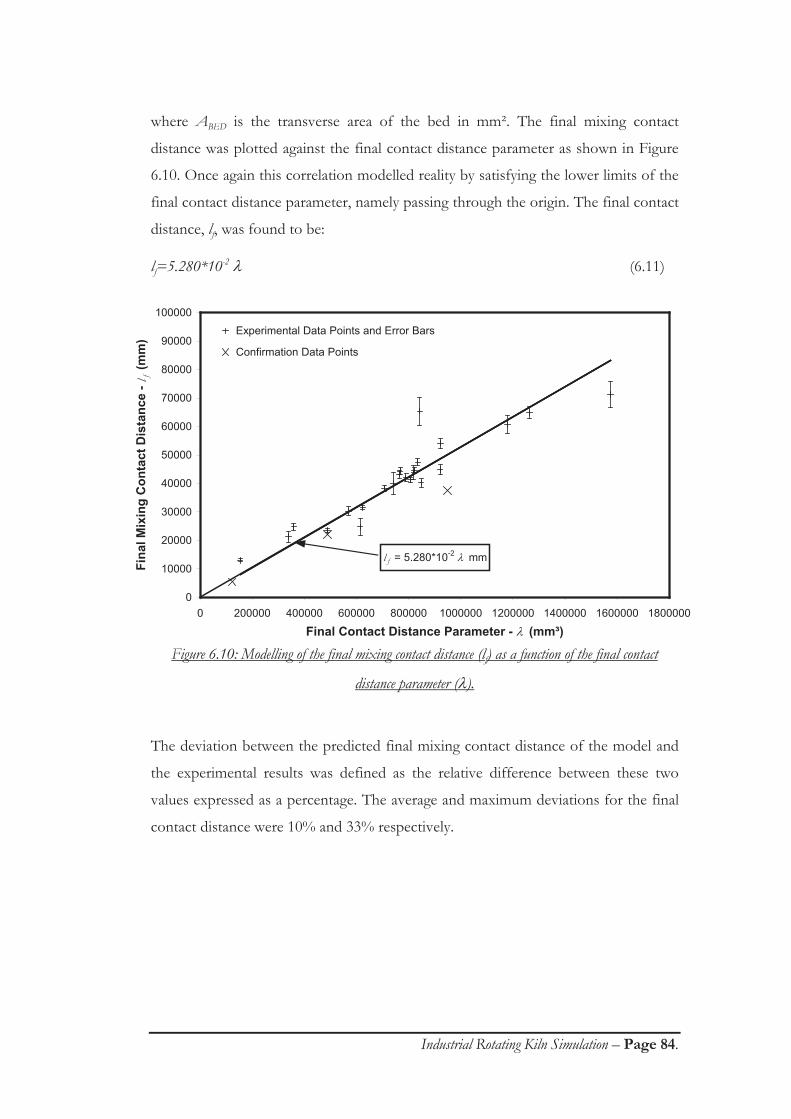
Industrial Rotating Kiln Simulation – Page 84.
where ABED is the transverse area of the bed in mm². The final mixing contact
distance was plotted against the final contact distance parameter as shown in Figure
6.10. Once again this correlation modelled reality by satisfying the lower limits of the
final contact distance parameter, namely passing through the origin. The final contact
distance, lf, was found to be:
lf=5.280*10-2 (6.11)
l f = 5.280*10-2 mm
0
10000
20000
30000
40000
50000
60000
70000
80000
90000
100000
0 200000 400000 600000 800000 1000000 1200000 1400000 1600000 1800000
Final Contact Distance Parameter - (mm³)
Fina
l Mix
ing
Con
tact
Dis
tanc
e - l
f (m
m)
Experimental Data Points and Error Bars
Confirmation Data Points
Figure 6.10: Modelling of the final mixing contact distance (lf) as a function of the final contact
distance parameter ( ).
The deviation between the predicted final mixing contact distance of the model and
the experimental results was defined as the relative difference between these two
values expressed as a percentage. The average and maximum deviations for the final
contact distance were 10% and 33% respectively.

Industrial Rotating Kiln Simulation – Page 85.
6.6 APPLICATION AND VERIFICATION OF THE MIXING
MODEL
The mixing model of solids in a rolling bed of a rotating drum consists of two
parameters, the determination of the mixing rate and the final contact distance of the
bed. In order to use the mixing model, the bed must to be characterised so that the
active layer parameter and the final contact distance parameter can be calculated.
Thus the active layer percentage as modelled earlier needs to be predicted. From this
value the active layer velocity and the active layer area can be calculated. The mean
particle size and the material ratio should be known from the experimental setup.
Once the active layer parameter is determined, the mixing rate can be calculated. To
determine the final contact distance between the two different materials, the final
contact distance parameter needs to be calculated. This is done using the bed
specifications. By combining the final contact and the mixing rate, the time required
to obtain a fully mixed bed can be determined.
Results from Experiments 25 to 27 are shown in Figures 6.9 and 6.10 as the
confirmation data points. These experiments were used to test the applicability of the
mixing model. Experiment 25 was used to test a different configuration of the bed.
The configuration used in experiment 25 conformed to the “smile” configuration as
shown in Figure 4.4a with the orange material on the outside of the black material.
Experiments 26 and 27 were carried out in smaller drums of 400 mm and 200 mm
diameter respectively, and these results were used to validate the scaling capabilities
of the model.
The mixing rates of the experiments carried out in the smaller drums were predicted
to within 3% of the experimental mixing rates. This was less than the average
experimental mixing rate error of 12%. However the determination of the mixing
rate of Experiment 25 was 19%. This is still less than the maximum experimental
error of the mixing rate experiments. For Experiments 25 to 27, the final contact
distance predicted from the model was greater than the experimentally measured

Industrial Rotating Kiln Simulation – Page 86.
final contact distance. The deviations were larger than the average deviation of the
final contact distance model but within the maximum deviation of the final mixing
contact distance model.
The successful scaling of the mixing model, using Experiments 26 & 27, was
attributed to the use of the active layer proportion correlation of Chapter 5. The
model derived here was only tested at the end of a rotational drum but could predict
the mixing behaviour in the bulk of a rolling bed if the active layer characteristics in
the bulk of the bed are known. Boateng & Barr (1997) noted that the active layer
becomes larger away from the end wall indicating a lower velocity. From the active
layer parameters this would indicate a slower mixing rate in the bulk of the bed
compared to the mixing rate observed at the wall.
6.6 TRANSVERSE MIXING SUMMARY
A new experimental method has been developed to measure the mixing of solids in a rotary kiln
using image analysis. Images were taken of the rotating bed and a program was written to analyse
these images to determine the contact distance between the different coloured materials.
The experiments carried out tested rotational velocities from 5 to 19 rpm, particle sizes from 0.89 to
5.08 mm, drum loadings from 6 to 40 % by volume and material ratios from 0.55 to 2.70. The
mixing rate and the final contact distance were measured from the mixing experiments.
It was observed that the mixing rates for all experiments were linear in nature. Closer observations
showed that this linearity was made up from a series of steps. Increases in mixing rates were due to
increased rotational velocity and drum loading, while decreases in mixing rate were due to increased
particle size and material ratio. The mixing rates were modelled with respect to an active layer
parameter, which in turn was a function of the mean active layer velocity, the transverse area of the
active layer, the particle size and the material ratio. A linear relationship was found between this
active layer parameter and the mixing rate in the drum.
Industrial Rotating Kiln Simulation – Page 87.
The final contact distance did not vary with rotational speed but increased with increased drum
loadings, decreased by increasing the particle size and decreased by increasing the material ratio. The
final contact distance was modelled as a function of the final contact distance parameter, which was a
function of the transverse bed area, the particle size and the material ratio. A linear relationship was
determined for the final contact distance calculation.
The derived models were tested on independent experiments. These independent experiments were
carried out for different bed configurations and different drum sizes. Accurate predictions were made
of the experimental mixing rates and final contact distances using the models derived in this chapter.
These models allow a quantitative measure of the mixing behaviour in a rotating drum to be
predicted.
Industrial Rotating Kiln Simulation – Page 88.
CHAPTER 7
Segregation in the transverse direction of a rotating drum.
Segregation of solids occurs when solid particles of varying sizes and/or densities are
mixed. The size and/or density differences result in the heavier and/or smaller
particles being concentrated toward the centre of the solid bed in a rolling drum to
form a segregated core. Figure 7.1 shows a rolling bed illustrating the position of the
segregated core. Segregation has important energy efficiency implications in the
operation of industrial rotating kilns (Barr et al, 1989a, b) by hindering heat transfer
from the flame in the gaseous phase to the segregated core.
Figure 7.1: Rolling bed showing segregated core and the centre of rotation.
In this chapter a model is developed to predict transverse segregation of granular
material in a rolling drum. Previous work (Pollard & Henein, 1989) has shown that
the particle size ratio and the rotational velocity strongly affect the segregation
behaviour of solid flows. In this work, the effects of the particle size ratio and the
mean active layer velocity are studied. The mean active layer velocity was used as this

Industrial Rotating Kiln Simulation – Page 89.
would represent the velocity of the material in the active layer, where the segregation
occurs. Experiments were carried out to measure the effect of these parameters on
the segregation dynamics and the final extent of transverse segregation. These
experimental results were used to derive a predictive model of transverse segregation.
7.1 TRANSVERSE SEGREGATION EXPERIMENTS
Coloured shale with mean particle sizes as shown in Table 7.1 was used in the
experiments. The bulk densities of the different sized coloured material were given in
Table 4.3 and it was found that these were not significantly different. Thus
segregation due to density differences, as shown by Ristow (1994) would not occur.
The particle size ratios tested ranged from 5.71, for the 5.08 and 0.89 mm material, to
1.37, for the 3.44 and 2.51 mm material. Material less than 0.60 mm diameter was not
used in this work due to the inability to colour such small particles. However, it was
assumed that due to their electrostatic properties, the smallest particle size would
adhere to the surface of the larger particles and thus not take part in segregation.
This assumption was made based on the observations of Bridgewater (1976).
Rotational velocities were varied in the experiments from 3 to 23 rpm. The lowest
velocity coincided with the start of the rolling regime whereas the highest velocity
occurred at the maximum rotational speed of the experimental drum. The transverse
segregation experiments and results are presented in Table 7.1.
Images of the bed were taken to measure both the segregation dynamics and the final
segregated configuration. The initial configuration of the bed for the segregation
dynamics experiments was a well mixed bed. After the bed was loaded, with well
mixed material, and the glass panel replaced, rotation was started and images of the
drum were taken from the initially well mixed condition until the final segregated
state. For the segregation dynamics experiments, images were taken every second for
60 seconds whilst the bed was in motion. For the final segregated state

Industrial Rotating Kiln Simulation – Page 90.
Experiment Number
Particle Size Ratio
Drum Rotational Velocity
NSegregation
Time
Final Inner Layer
Concentration Proportion
Final Outer Layer
Concentration Proportion
UNITS mm/mm rpm s - -28a 1.37 2.91 2.0 1.21 0.9228b 1.37 5.73 3.5 1.25 0.9128c 1.37 8.47 2.5 1.18 0.9328d 1.37 12.51 - 1.16 0.9428e 1.37 17.51 - 1.12 0.9628f 1.37 23.23 - 1.08 0.9729a 1.48 2.90 3.0 1.01 1.0029b 1.48 4.76 - 1.09 0.9729c 1.48 6.70 - 1.09 0.9729d 1.48 8.47 - 1.10 0.9629e 1.48 10.56 - 1.10 0.9729f 1.48 12.51 - 1.09 0.9729g 1.48 14.94 - 1.08 0.9729h 1.48 17.51 - 1.07 0.9729i 1.48 20.34 - 1.06 0.9829j 1.48 23.23 - 1.05 0.9830a 1.91 2.90 5.0 1.49 0.8230b 1.91 5.72 2.5 1.36 0.8730c 1.91 8.46 3.5 1.29 0.8930d 1.91 12.50 - 1.25 0.9130e 1.91 17.49 - 1.20 0.9330f 1.91 23.21 - 1.12 0.9631a 2.02 3.89 5.0 1.48 0.8231b 2.02 6.73 1.5 1.34 0.8731c 2.02 9.64 - 1.29 0.8931d 2.02 13.64 - 1.22 0.9231e 2.02 21.71 - 1.13 0.9532a 2.82 2.90 8.0 1.84 0.6932b 2.82 5.72 6.0 1.45 0.8332c 2.82 8.46 3.5 1.45 0.8332d 2.82 12.49 - 1.36 0.8632e 2.82 17.49 - 1.24 0.9132f 2.82 23.21 - 1.13 0.9633a 2.99 2.87 - 1.91 0.6733b 2.99 6.67 - 1.71 0.7433c 2.99 10.51 - 1.52 0.8133d 2.99 14.87 - 1.40 0.8633e 2.99 20.27 - 1.25 0.9134a 5.71 2.48 - 1.94 0.6634b 5.71 5.62 - 1.73 0.7434c 5.71 8.38 - 1.60 0.7834d 5.71 11.22 - 1.56 0.8034e 5.71 15.81 - 1.36 0.8734f 5.71 21.30 - 1.22 0.92
Average Error 2.5% 1.5%Minimum Error 0.7% 0.3%Maximum Error 5.3% 4.8%
351 3.87 10.55 - 1.67 0.7536a1 2.02 2.99 - 1.80 0.7236b1 2.02 13.77 - 1.32 0.89
NOTES:1) These experiments were carried out to test the model based on experiments 28 through 34.
Table 7.1: Segregation experiments and results.

Industrial Rotating Kiln Simulation – Page 91.
experiments, 20 images were taken after the bed had been rotating for a minute and
had attained its final segregated configuration. These images were taken whilst the
bed was in motion. After development, the images were analysed to determine the
amount of segregation of each image, as explained below. All experiments were
carried out in the rolling regime, as this is the desired motion regime of an industrial
rotating kiln.
7.2 EXPERIMENTAL ANALYSIS METHODOLOGY
Segregation of the fine material occurred such that the fine material moved towards
the rotational centre of the bed. In order to measure the segregation, the segregation
analysis software measured the concentrations of the different coloured particles at
various distances from this rotational centre. This methodology is outlined in this
section of the thesis.
Before the materials could be allocated to different zones of the bed, the geometry of
the rolling bed needed to be recorded. This was achieved by defining the edges of the
rolling bed. A typical image representing the development of the bed regime for each
experiment was manually selected. The centre of rotation of the selection was
determined after specifying the locations of Apex A and Apex B of the image, as
shown in Figure 7.2, using the equations derived in Chapter 5. From this centre of
rotation an array was constructed which contained data of both the distance from the
centre of rotation to the selection edge and the angle at the centre for all points of
the selection. This array, called the bed outline, was sorted, reduced in size to speed
up image processing, saved and used in the analysis of the experimental images. The
data was selectively reduced to ensure that the loss of information for the bed outline
was minimal. Figure 7.2 shows a typical example of the bed outline. Furthermore,
Figure 7.2 also shows the division of layers, the inner layer representing 50% of the
radius of the bed outline at any angle from the rotational centre.
For each image in an experiment, Apex A and Apex B were manually located. From
the specification of these points the centre of rotation of the current image was
determined. The distance and the angle for the pixels of the image were calculated
and compared with the data in the bed outline array. If the distance of the current

Industrial Rotating Kiln Simulation – Page 92.
pixel occurred outside the bed outline radius at the calculated angle, the pixel was
ignored. It the pixel occurred within the bed outline radius the count of that pixel
type, in the layer in which the pixel occurred, increased by 1.
-1000
-800
-600
-400
-200
0
200
400
600
800
-2000 -1500 -1000 -500 0 500 1000 1500 2000
X distance from centre of rotation in pixels
Y di
stan
ce fr
om c
entr
e of
rota
tion
in p
ixel
s
Inner Layer Outer Layer
Centre of rotation
Apex B
Apex A
Z
X
Y
BED OUTLINE
Figure 7.2 – Bed outline used in the segregation analysis.
An example is given to clarify the segregation analysis mechanism. Consider that a
typical image was scanned and the current pixel being analysed corresponds to point
Z in Figure 7.2. This occurred at angle . The distance from the centre of rotation of
the bed to Z was compared to the radius of the bed outline at that angle, . The
distance to Z was greater than the outline radius and hence point Z was not included
in the count of valid data points. When point Y, which was assumed to be orange,
was encountered, it was found that this point occurred within the outline. In fact it
occurred in the outer layer and thus the orange count of the outer layer was increased
by 1. Point X was dealt with similarly but increased the count of its colour type in the
inner layer.
By applying the image analysis method to the whole image, the total count of orange
and black pixels in each layer was measured. A concentration proportion, defined as
the ratio of the concentration of the segregating material in each layer to the mean
concentration of the segregated material in the bed, was used to express the

Industrial Rotating Kiln Simulation – Page 93.
distribution of the segregating material. For the jth layer, the concentration
proportion, Pj, was defined as:
)()(ttt
jjjj
BOOBOOP (7.1)
where Oj was the count of orange pixels – representative of the smaller particles - in
the jth layer, Bj was the count of black pixels – representative of the larger particles -
in the jth layer, Ot was the total count of orange pixels in the bed and Bt was the total
count of black pixels in the bed.
Comparing this data for different images at different times allowed the segregation
dynamics to be determined. It should be noted here that numerous layers could be
used in the image analysis method to obtain a more defined distribution of fine
particles in the bed. However when using more than 2 layers the computational time
increased significantly and the accuracy decreased, especially for the inner layers, due
to the smaller sample size of the inner layer.
7.3 EXPERIMENTAL SEGREGATION RESULTS
The segregation results consisted of both the dynamics of segregation, taken as the
time for the bed to reach its final segregated composition from an initially well mixed
bed and the final segregated composition of the bed.
The segregation occurred too fast to be measured and hence the segregation
dynamics were only observed in a few experiments. Due to this, no correlation
between segregation time, particle size ratio and rotational velocity could be derived.
The segregation times, when they could be measured, were taken as the time required
to reach the fully segregated bed from the initially well mixed bed and are shown in
Table 7.2. Figure 7.3 illustrates typical segregation results when the segregation time
could be measured.

Industrial Rotating Kiln Simulation – Page 94.
0.0
0.2
0.4
0.6
0.8
1.0
1.2
1.4
1.6
1.8
2.0
0 2 4 6 8 10 12 14 16 18 20
Time (s)
Fine
Mat
eria
l Con
cent
ratio
n Pr
opor
tion(
-) Outer Layer Concentration Proportion Inner Layer Concentration Proportion
Segregation Time
Final Outer Layer Concentration Proportion
Final Inner Layer Concentration Proportion
Concentration proportion of 1.00
Figure 7.3: Results from a typical segregation experiment.
The final segregated concentration proportion was calculated as the average of the
concentration proportions in each layer for the 20 images taken of the fully
segregated bed. This corresponds to the average of the fine material concentration
proportion after the initial segregation time as shown in Figure 7.3. The fine material
was found to move towards the center of the bed for all experiments but this
tendency was reduced with the use of smaller particle size differences and higher
active layer velocities.
The experimental final concentration proportion is shown in Table 7.1 for both the
inner and outer layers of the bed. For all experiments it was observed that the final
extent of segregation decreased as the rotational velocity increased. Typical bed
configurations for experiment 32 with the different rotational velocities are shown in
Figure 7.4. Figure 7.4 A corresponds to the final bed configuration of experiment
32a.

Industrial Rotating Kiln Simulation – Page 95.
a) 2.90 rpm, b) 5.72 rpm, c) 8.46 rpm, d) 12.49 rpm, e) 14.87 rpm and f) 23.21 rpm
Fig 7.4: Sample final segregation beds for experiment 32.
7.4 ANALYSIS OF THE SEGREGATION RESULTS
The active layer was described in Chapter 5. Using the active layer parameters allows
the experimental results to be easily compared and applied to different rotating kilns
as shown with the mixing modelling of Chapter 6. Hence the segregation modelling
will also be based on the active layer properties. The active layer proportion and
active layer velocity are calculated for the segregation experiments and shown in
Table 7.2.

Industrial Rotating Kiln Simulation – Page 96.
7.4.1 Segregation dynamics
Experiment 31a used a particle size ratio of 1.91, a rotational velocity of 2.90 rpm
and a drum loading of 15%. This corresponded to an active layer velocity of 0.36
m/s. The segregation time for experiment 31a, as shown in Table 7.1, was 5.00
seconds. For the experimental conditions of experiment 31a, the bed of particles
rotated approximately once every 5 seconds, which corresponded to the measured
segregation time. However, it must be noted that the experiments were started with
an initial stationary bed and that it took a few seconds for the rolling regime to
become fully developed in the bed. Thus the bed was fully segregated within one bed
revolution. This behaviour was observed for all segregation experiments and
indicated that segregation was completed as the granular material passed through the
active layer.
At higher rotational velocities the segregation times were not measured since the
segregation occurred too fast to be observed. The faster segregation rates found in
this work when compared to other work in the literature can be explained by noting
the observations of Pollard & Henein (1989) who found that the segregation rate was
significantly faster in a 400 mm diameter drum than in a 200 mm diameter drum. The
mean active layer velocity in Pollard & Henein’s (1989) 200 mm drum was 0.247 m/s
whereas it was 0.266 m/s in their 400 mm drum. A drum of 570 mm diameter was
used in the current work and the mean active layer velocities were greater than 0.34
m/s in all experiments. Thus the segregation times decreased as the active layer
velocity increased. This result can be extended to industrial drums by assuming that
the segregation dynamics are completed within a single bed revolution at higher
active layer velocities such as those experienced in large industrial rotating drums.
Furthermore, as will be shown below, the use of the higher active layer velocities
reduced the amount of segregation due to the higher mixing rates as observed in
Chapter 6.

Industrial Rotating Kiln Simulation – Page 97.
Experiment Number
Active Layer Proportion
%ALActive Layer
Velocity
Predicted Inner Layer
Concentration Proportion
Predicted Outer Layer
Concentration Proportion
UNITS - m/s - -28a 20 0.34 1.17 0.9428b 27 0.47 1.15 0.9528c 31 0.57 1.13 0.9628d 34 0.71 1.11 0.9728e 38 0.86 1.09 0.9828f 41 1.02 1.07 0.9929a 20 0.35 1.21 0.9329b 25 0.43 1.19 0.9429c 28 0.51 1.18 0.9429d 30 0.58 1.16 0.9529e 33 0.65 1.15 0.9629f 34 0.72 1.14 0.9629g 36 0.79 1.12 0.9729h 38 0.87 1.11 0.9729i 39 0.95 1.09 0.9829j 40 1.02 1.07 0.9930a 20 0.36 1.39 0.8630b 26 0.48 1.33 0.8830c 30 0.59 1.29 0.9030d 34 0.73 1.23 0.9230e 37 0.88 1.16 0.9530f 40 1.04 1.09 0.9831a 19 0.48 1.37 0.8731b 25 0.61 1.31 0.8931c 28 0.73 1.25 0.9131d 32 0.88 1.17 0.9431e 36 1.14 1.04 0.9932a 20 0.35 1.77 0.7132b 26 0.47 1.66 0.7632c 30 0.58 1.56 0.7932d 34 0.72 1.42 0.8432e 37 0.87 1.28 0.8932f 40 1.03 1.13 0.9533a 20 0.34 1.86 0.6833b 28 0.50 1.69 0.7433c 33 0.64 1.55 0.7933d 36 0.78 1.41 0.8533e 39 0.93 1.25 0.9034a 14 0.46 1.83 0.7034b 22 0.59 1.68 0.7534c 26 0.71 1.56 0.8034d 29 0.83 1.44 0.8434e 32 1.00 1.27 0.9034f 35 1.18 1.08 0.97
Average Deviation 4.6% 2.6%Minimum Deviation 0.2% 0.0%Maximum Deviation 19.4% 9.1%
351 33 0.65 1.63 0.7736a1 17 0.43 1.40 0.8636b1 32 0.86 1.18 0.94
NOTES:1) These experiments were carried out to test the model based on experiments 28 through 34.
Table 7.2: Calculated segregation parameters used in the segregation modelling.

Industrial Rotating Kiln Simulation – Page 98.
7.4.2 The final segregated bed
A typical experimental plot of the final segregated concentration proportion for
experiments 30a to 30f is shown in Figure 7.5. The error bars shown on Figure 7.5
represent the experimental error from the average value. For larger particle size
ratios, the bed had a higher concentration proportion of the fine material in the inner
layer and a lower concentration proportion in the outer layer.
0.60
0.80
1.00
1.20
1.40
1.60
1.80
0.00 0.20 0.40 0.60 0.80 1.00 1.20
Mean Active Layer Velocity (m/s)
Fina
l Seg
rega
ted
Con
cent
ratio
n Pr
opor
tion(
-)
Inner Layer Concentration Proportion Outer Layer Concentration Proportion
Concentration proportion of 1.00
Inner layer line of best fit."Line of best fit" intercept, i i (PSR)
"Line of best fit" gradient, m i (PSR)
)().( PSRiVPSRmP iALii
Figure 7.5:Concentration proportion for the inner and outer layer for experiments 30a to 30f.
The average experimental errors for the final inner and outer layer concentration
proportion for all experiments were 2.5 and 1.5 % respectively and the maximum
errors were 5.3 and 4.8 % respectively. It should be noted that the errors in the inner
layer were larger than the errors in the outer layer since the inner layer consisted of a
significantly smaller sample size and thus any fluctuations became more prominent.

Industrial Rotating Kiln Simulation – Page 99.
7.5 MODELLING OF THE SEGREGATION IN THE
TRANSVERSE DIRECTION OF A ROLLING DRUM
The results from Table 7.1 show that decreasing the particle size ratio reduced the
extent of segregation. This was expected since the ease by which smaller particles
percolated through the voids was dependent on the size of the voids. Williams &
Khan (1973) found that the size of these voids was dependent on the size of the
larger particles. Figure 7.5 shows a linear relation between the active layer velocity
and the final segregated concentration proportion for experiments 30a to 30f. The
linear relation has the form:
jALjj iVmP . (7.2)
where ALV was the mean active layer velocity, mj and ij were the gradient and
intercept for the “line of best fit”.
Analysis of the other particle size ratios produced graphs similar to Figure 7.5 but
with different gradients and intercepts for the line of best fit. It was noted that the
“lines of best fit” became steeper with larger particle size ratios, which indicated that
mj and ij were only functions of particle size ratio and Equation 7.2 can be rewritten
as:
)().( PSRiVPSRmP jALjj (7.3)
where mj(PSR) and ij(PSR) were the gradient and intercept functions for the different
particle size ratios respectively.
The model developed predicted the gradient and the intercept functions of the
concentration proportion for each set of particle size ratios. Figure 7.6 shows the
different values of the gradient and the intercept of the “lines of best fit” for each
particle size ratio range for the inner layer. To ensure that the model was physically
realistic with respect to the known and experimental boundary conditions, i.e. for a
particle size ratio of 1, no segregation occurs in the bed, the gradient correlation was
forced through 0 and the intercept correlation was forced through 1 at this particle
size ratio. Limiting values of the gradient and intercept were observed at higher
particle size ratios and are shown in Figure 7.6 as the final gradient and the final
Industrial Rotating Kiln Simulation – Page 100.
intercept respectively. These were obtained by averaging the final values of the
gradient and intercept of the “lines of best fit” for the larger particle size ratio
experiments. The values of the gradient and intercept needed to be determined so
that the concentration proportion could be determined using Equation 7.3.
As can be seen from Figure 7.6, there was a small range of particle size ratio, close to
1, where no segregation was observed and thus the values of mj(PSR) and ij(PSR)
were equal to the values at the boundary conditions. A final limit was also observed
for the larger particle size ratios, such as those greater than 2.92. The region in
between these limits was linear and can be easily correlated.
-1.20
-1.00
-0.80
-0.60
-0.40
-0.20
0.000 1 2 3 4 5 6
Particle Size Ratio
Gra
dien
t (PS
R)
0.00
0.50
1.00
1.50
2.00
2.50
Inte
rcep
t (PS
R)
Gradient Data PointsIntercept Data Points
Intercept = 1.00
Gradient = 0.00
Final InterceptFinal Gradient
Figure 7.6: Modelling of m(PSR) and i(PSR) for the inner layer.
The prediction of mj(PSR) and ij(PSR) needed to be within the ranges of the
boundary conditions and the final points for the model to be useful. Table 7.3
illustrates how the values of the gradients and intercepts were calculated for each
layer. The data from Table 7.2 were used to calculate the accuracy of the model by
predicting the concentration proportion for each of the experiments used in the
model derivation. The deviation, expressed as an absolute percentage between the
experimental concentration proportion and the value predicted form the model, was

Industrial Rotating Kiln Simulation – Page 101.
calculated for each experimental data point. The average deviation for the inner layer
prediction was 4.6% and for the outer layer this average deviation was 2.6%. These
deviations are 1-2 % higher than the average experimental errors but are within the
maximum experimental error range, which was 5.3 % for the inner layer and 4.8%
for the outer layer. For the 44 experiments carried out, 13 model predictions for the
inner layer and 6 model predictions for the outer layer had an error deviation larger
than the maximum experimental errors. These larger errors occurred at the
extremities of the data sets, such as at the lowest and highest velocities. This is due to
the limited overlap of experimental data that are normally associated with the
extremities of data sets.
Lower Limit
PSR Dependent Range
Upper Limit
m(PSR) -1.03 -0.56 * PSR + 0.62 0.00i(PSR) 1.00 0.61 * PSR + 0.37 2.29
m(PSR) 0.00 0.19 * ( PSR - 1) 0.38i(PSR) 0.53 -0.23 * PSR + 1.23 1.00
Inner Layer
Outer Layer
Table 7.3: Parameters used in the segregation model.
7.6 APPLICATION AND VERIFICATION OF THE
SEGREGATION MODEL
Experiments 35, 36a and 36b were carried out but not included in the data set used
for the modelling of the segregation. These experiments were used as independent
experiments to test the predictive capability of the developed segregation model. The
experimental conditions, experimental results and predicted modelling results are
shown in Tables 7.1 and 7.2 respectively.
The deviation between the model prediction and the experimental results were
calculated and are shown in Table 7.4. For Experiment 35 the model deviations for
both the inner and outer layer were less than the average deviation of the segregation
model. For experiment 36a the deviation for the inner layer prediction was 22.2%
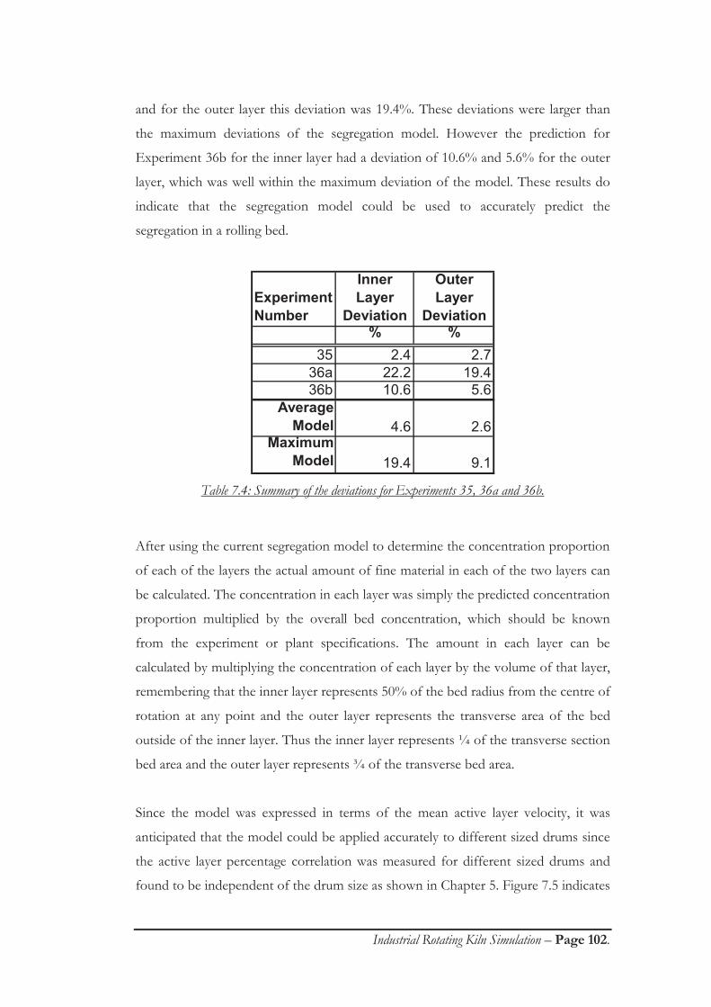
Industrial Rotating Kiln Simulation – Page 102.
and for the outer layer this deviation was 19.4%. These deviations were larger than
the maximum deviations of the segregation model. However the prediction for
Experiment 36b for the inner layer had a deviation of 10.6% and 5.6% for the outer
layer, which was well within the maximum deviation of the model. These results do
indicate that the segregation model could be used to accurately predict the
segregation in a rolling bed.
Experiment Number
Inner Layer
Deviation
Outer Layer
Deviation% %
35 2.4 2.736a 22.2 19.436b 10.6 5.6
Average Model 4.6 2.6
Maximum Model 19.4 9.1
Table 7.4: Summary of the deviations for Experiments 35, 36a and 36b.
After using the current segregation model to determine the concentration proportion
of each of the layers the actual amount of fine material in each of the two layers can
be calculated. The concentration in each layer was simply the predicted concentration
proportion multiplied by the overall bed concentration, which should be known
from the experiment or plant specifications. The amount in each layer can be
calculated by multiplying the concentration of each layer by the volume of that layer,
remembering that the inner layer represents 50% of the bed radius from the centre of
rotation at any point and the outer layer represents the transverse area of the bed
outside of the inner layer. Thus the inner layer represents ¼ of the transverse section
bed area and the outer layer represents ¾ of the transverse bed area.
Since the model was expressed in terms of the mean active layer velocity, it was
anticipated that the model could be applied accurately to different sized drums since
the active layer percentage correlation was measured for different sized drums and
found to be independent of the drum size as shown in Chapter 5. Figure 7.5 indicates

Industrial Rotating Kiln Simulation – Page 103.
that at mean active layer velocities beyond 1.20 ms-1 reverse segregation would occur.
However, Nityanand et al (1986) showed that reverse segregation only occurred
when the bed was operated in the centrifuging regime. Thus, at higher active layer
velocities segregation will not take place in a rolling bed.
7.7 CHAPTER SUMMARY
A new method, using image analysis, was developed in this chapter to measure the segregation of
solids in the transverse section of a rotating drum, operating in the rolling regime. This new data
analysis method was applied to various experiments to study the effect of particle size ratio and mean
active layer velocity on both the segregation dynamics and the final segregated configuration.
The segregation dynamics were only observable for a few experiments and therefore could not be
modelled. However, by comparing the present work to earlier work showed that segregation occurred
faster in larger drums due to the increase of the mean active layer velocity. From these studies it was
assumed that the time for the material to fully segregate in an industrial rotating drum would be very
short due to the higher active layer velocities experienced in industrial rotating drums.
The derived correlations for the final concentration proportions to determine the concentration
proportions were dependent on the active layer velocity and the particle size ratio. Comparison of the
experimental results and model predictions showed that the model could be applied accurately.
Further to this, the active layer velocity can be predicted for different sized rotating drums using the
results of Chapter 5 and thus the segregation model can be applied to predict the segregation
behaviour of solids in different sized rotating drums.

Industrial Rotating Kiln Simulation – Page 104.
CHAPTER 8
Simulation of the mixing and segregation of solids in the
transverse section of a rotating drum.
In this chapter the behaviour of the solid mixing and segregation in the transverse
section of a rotating drum was simulated. This involved the design of a suitable grid
to represent the transverse section of a rolling drum and the translation of the
models derived in Chapters 6 & 7 to suit this grid. The simulation was tested against
experimental data.
As described in Chapter 3, the transverse section of a rolling bed consisted of an
‘active layer’ and a ‘stagnant layer’. The behaviour of the solids in these layers was
different and hence different elements were required to simulation of these layers.
8.1 “STREAM” DEFINITION
The simulation used an approach between classical lumped parameter modelling and
discrete elemental analysis modelling. A “stream” was defined as an entity that
consisted of flow rates for a range of materials, each of which could be at a different
temperature. The amount of mixing between the materials was also included in a
“stream”. The best way to illustrate the “stream” was to include the C++ computer
code of a “stream” as shown in Figure 8.1.
The “stream” variable consisted of an array of ASH and SHALE material variables.
ASH and SHALE were used in the “stream” definition to represent the two different
materials present in the retort zone of the AOSTRA-Taciuk Processor. These arrays
represented the different material sizes, their flow rates and their temperatures. For
example, ASH[ 0] corresponded to the smallest ash size. Since the material size was

Industrial Rotating Kiln Simulation – Page 105.
used in the definition, the material size was not required in the “stream” structure.
The flow of the material, FLOW, and the temperature, TEMP, in each “stream”
could be specified. FLOW was measured in m²/sec and TEMP was measured in K.
TEMP is used in the granular heat transfer and will be described in Chapter 9.
struct Material{
double FLOW;double TEMP;
};
class Stream{
public:double ExtentOfMixing;// ASH and SHALE streams of the following particle ranges// -0.60, +0.60-1.40, +1.40-2.00, +2.00-3.02, +3.02-3.86, +3.86-6.30// ASH[ 0] refers to 0-0.60 mm, ASH[ 1] refers to 0.60-1.40 mm etcMaterial ASH[ 7];Material SHALE[ 7];
};
Figure 8.1: C++ computer code for the definition of the “stream” structure.
These “streams” were used in the ‘stagnant layer’ and the ‘active layer’ control
volumes as described below.
8.2 ‘STAGNANT LAYER’ CONTROL VOLUMES
The ‘stagnant layer’ control volume represented an element of residence time only
since no mixing or segregation occurred within the ‘stagnant layer’, as shown in the
experiments and the literature review. However, heat transfer between the two
materials and the volatile evolution from the shale occurred in the ‘stagnant layer’
and this will be considered in Chapter 9.

Industrial Rotating Kiln Simulation – Page 106.
Figure 8.2 shows a schematic of the ‘stagnant layer’ control volume. The size of the
control volume was dependent on the geometry of the drum and only two “streams”
occurred within the ‘stagnant layer’ control volume. These “streams” were the
Stagnant Layer Feed and the Stagnant Layer Product. In the current simulation, the
Stagnant Layer Product equalled the Stagnant Layer Feed but with a time delay. This
time delay and the geometry of the control volumes will be described in Section 8.5.
The temperatures of the “streams” will differ in Chapter 9 due to the inclusion of the
heat transfer mechanism and the volatile evolution of the shale. The volatile
evolution of Figure 8.2 is not defined as a “stream”. The volatile evolution represents
the volatiles evolved from that control volume as calculated using the imbedded heat
transfer and volatile evolution models of Chapter 9.
Volatile Evolution
Stagnant Layer Heat Transfer Stagnant LayerFeed Volatile Evolution Product
'Stagnant Layer' Control Volume
Figure 8.2: Schematic of a ‘stagnant layer’ control volume.
The ‘stagnant layer’ control volume was also defined as a “stream”. Each ‘stagnant
layer’ control volume contained functions to determine the important parameters of
the control volume. These functions allowed the mean particle sizes, the mean
temperatures and the total flows of the materials to be calculated.
8.3 ‘ACTIVE LAYER’ CONTROL VOLUMES
An ‘active layer’ control volume represented a small part of the ‘active layer’. It was
shown in Chapters 6 and 7 that the ‘active layer’ was responsible for the mixing and
segregation in the bed. Thus procedures were required to allow these mechanisms to
occur in the ‘active layer’ control volumes.

Industrial Rotating Kiln Simulation – Page 107.
The ‘active layer’ control volume had the same basic structure as the ‘stagnant layer’
control volume but had extra “streams” and included mixing and segregation
mechanisms. Figure 8.3 illustrates an ‘active layer’ control volume.
Volatile Evolution
Top Product Mixing Top FeedSegregation
Heat TransferBottom Product Volatile Evolution Bottom Feed
Stagnant Layer Stagnant LayerProduct Feed
'Active Layer' Control Volume
Figure 8.3: Schematic of an ‘active layer’ control volume.
8.3.1 Streams of the ‘active layer’ control volume
Each ‘active layer’ control volume had a maximum of three “streams” as feeds.
These could be a “stream” from the ‘stagnant layer’, a “stream” from either the
upper or lower control volume of the previous ‘active layer’ control volumes. A
maximum of three product “streams” also existed for each ‘active layer’ control
volume. There was a possible feed to the stagnant layer or either an upper or lower
feed to the next ‘active layer’ control volumes. The number of “streams” depended
on the position of the control volume within the ‘active layer’.
8.3.2 Mixing in the ‘active layer’ control volume
The mixing model derived in Chapter 6 was directly applied to the solids in an ‘active
layer’ control volume. It was assumed that applying the mixing model derived for the

Industrial Rotating Kiln Simulation – Page 108.
complete ‘active layer’ to individual ‘active layer’ control volumes allowed the overall
mixing behaviour of the ‘active layer’ to be determined. This model requires the
determination of the ‘active layer’ parameter, which is dependent upon the mean
velocity in the control volume, the transverse area of the control volume, the mean
particle size diameter and the ratio of materials in that control volume. Since the
mean velocity of the control volume is dependent on the size and position of the
control volume, the control volumes needs to be characterised, which will be
described in the grid selection section below. The cross sectional area of the ‘active
layer’ control volume was calculated from the geometry of the bed. The mean
particle size and the material ratio were calculated for each control volume in each
time step to account for the fluctuations in these parameters due to material flow.
The ‘active layer’ parameter was calculated and then the mixing rate was calculated
using Equations 6.8 and 6.9. The mixing rate was multiplied by the sampling time,
SAMP, to calculate the new amount of mixing in the control volume in that time
sample. This new amount of mixing was then added to the previous amount of
mixing in that control volume. The final mixing contact, lf, for the control volume
was determined using Equations 6.10 and 6.11, to ensure that mixing in the control
volume did not exceed the maximum contact for that control volume. Thus the
amount of mixing in a control volume, l(t), at time t was calculated as:
SAMPf ttllMINIMUMtl ).()1(,)( (8.1)
The addition or removal of material from an ‘active layer’ control volume added or
removed the respective amount of mixing to or from that control volume. These
values were stored in the ExtentOfMixing variable of “stream”.
8.3.3 Segregation in the ‘active layer’ control volume
The segregation model derived in Chapter 7 was applied to the ‘active layer’ control
volumes. It was assumed that the segregation of the ‘active layer’ as a single entity

Industrial Rotating Kiln Simulation – Page 109.
could be approximated by applying the segregation model to the individual ‘active
layer’ control volumes. For the segregation mechanism, the Stagnant Layer Product
and the Bottom Product of the ‘active layer’ control volume were considered as a
single “stream” and the segregating material favoured this combined “stream”. This
approach only required the determination of the segregated material proportion in
the segregating “stream” and, if segregation occurred, forced material greater than
the mean particle size to the Top Product “stream”. The movement of material as
such was essential to maintain the mass balance in the control volumes. The
proportion of the finer material was calculated using Equation 7.3 and Table 7.3 but
in the simulation the particle size ratio was taken as the ratio of the mean particle size
in the control volume divided by the particle size of the segregating material. Only
particle sizes less than the mean particle size were considered in the segregation
mechanism.
Segregation was assumed to only be dependent on the particle size differences. The
density differences between the ash and the shale were not considered since the
experimental work was based solely on size differences. Thus for the segregation
mechanism, the ash and the shale of the same size were considered as a single
material. After the segregation, this segregated material was re-divided into its ash
and shale components.
The segregation model derived in Chapter 7 assumed that a uniform active layer
velocity was encountered. From the velocity profile of Nakagawa et al (1992) and as
shown in Section 8.4, the velocity in the ‘active layer’ control volumes were different.
The experimental segregation model did illustrate that for a mean velocity, a certain
proportion of the finer material would move closer to the rotational centre of the
bed. From the ‘active layer’ control volume velocities, the segregation was
determined in the individual ‘active layer’ control volumes. The mean velocity in each
control volume was known from the mixing method and thus the ratio of each
material, moving closer to the centre or further away from the centre was calculated,
since numerous particle sizes were used in this work, which required numerous
segregation correlations to be solved simultaneously.

Industrial Rotating Kiln Simulation – Page 110.
Thus the proportion of each particle size for each material was calculated. The actual
material content into the “stream” depended on the control volume size, the flow of
the “streams” and the ratio of the segregating material.
8.4 SELECTION OF A GRID SYSTEM TO REPRESENT A
ROLLING BED
The grid of the control volumes used in the simulation, as shown in Figure 8.4,
consisted of the previously defined ‘stagnant layer’ and ‘active layer’ control volumes.
These control volumes were combined to represent the transverse section of a rolling
bed.
In order to discuss the grid a few definitions are required. ‘Stagnant layer’ and ‘active
layer’ control volumes were defined above and are illustrated by the individual
polygons of Figure 8.4. An ‘active layer’ zone consisted of the ‘active layer’ control
volumes between the ‘stagnant layer’ – ‘active layer’ interface and the free surface of
the bed. These were made up of 2 or 3 individual ‘active layer’ control volumes
representing the different layers within an ‘active layer’ zone. At the extremities of
the ‘active layer’, the ‘active layer’ zone only consisted of one ‘active layer’ control
volume. A ‘stagnant layer’ zone consisted of the ‘stagnant layer’ control volumes
between the edge of the bed and the centre of rotation. ‘Stagnant layer’ layers were
defined as the ‘stagnant layer’ control volumes between two annuli. These definitions
are illustrated in Figure 8.4. By using numerous control volumes it was anticipated
that the mixing, segregation, heat transfer and volatile evolution could be simulated
accurately, especially in larger kilns. The different layers allowed the segregation of
the materials to be predicted. The staggering of the ‘active layer’ control volumes
facilitated the bringing together of the materials and allowed them to mix. This new
approach allowed mixing to occur between layers as the materials passed through the
‘active layer’.
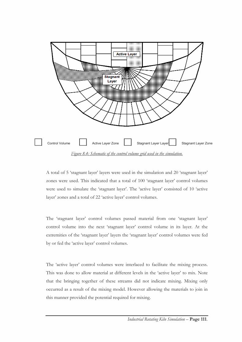
Industrial Rotating Kiln Simulation – Page 111.
Control Volume Active Layer Zone Stagnant Layer Layer Stagnant Layer Zone
Figure 8.4: Schematic of the control volume grid used in the simulation.
A total of 5 ‘stagnant layer’ layers were used in the simulation and 20 ‘stagnant layer’
zones were used. This indicated that a total of 100 ‘stagnant layer’ control volumes
were used to simulate the ‘stagnant layer’. The ‘active layer’ consisted of 10 ‘active
layer’ zones and a total of 22 ‘active layer’ control volumes.
The ‘stagnant layer’ control volumes passed material from one ‘stagnant layer’
control volume into the next ‘stagnant layer’ control volume in its layer. At the
extremities of the ‘stagnant layer’ layers the ‘stagnant layer’ control volumes were fed
by or fed the ‘active layer’ control volumes.
The ‘active layer’ control volumes were interlaced to facilitate the mixing process.
This was done to allow material at different levels in the ‘active layer’ to mix. Note
that the bringing together of these streams did not indicate mixing. Mixing only
occurred as a result of the mixing model. However allowing the materials to join in
this manner provided the potential required for mixing.

Industrial Rotating Kiln Simulation – Page 112.
8.5 SPECIFICATION OF THE SIMULATION
The sizes of the control volumes were calculated using the specifications of the
rotating drum. From the drum size and drum loading, the transverse bed area was
calculated. From the drum loading and the rotational velocity, the ‘active layer’
proportion was calculated using Equation 5.2. This allowed the total transverse area
of the ‘active layer’ and ‘stagnant layer’ to be calculated.
8.5.1 ‘Stagnant layer’ control volume characterisation
In the simulation, the ‘stagnant layer’ was assumed to consist of five individual layers.
It was assumed that the angle subtended by each of these layers at the centre of
rotation of the bed were equal. The areas of the different layers were calculated as a
proportion of the total bed area using a modified annulus area calculation method.
The five ‘stagnant layer’ layers were assumed to be equidistant. The area of the
individual ‘stagnant layer’ control volumes was obtained by dividing the area of the
‘stagnant layer’ layer by 20 as each layer was made up of 20 control volumes.
The velocities in the control volumes of a ‘stagnant layer’ layer were equal. These
were calculated at the mid chord position as the velocity at mid chord was linear as
shown by Nakagawa et al (1992). The rotational velocity of the drum at the drum
wall and the zero velocity point at the centre of rotation were used as the boundary
conditions and the mean velocities in the different layers were calculated by
interpolating between those boundary conditions.
The residence times in the ‘stagnant layer’ control volumes were determined from the
angular velocity of the drum and the angle subtended at the centre of rotation of the
‘stagnant layer’ control volumes. Since the ‘stagnant layer’ was well packed, all the
residence times of the ‘stagnant layer’ control volumes were assumed to be equal.
Industrial Rotating Kiln Simulation – Page 113.
A flux was developed in the ‘stagnant layer’. The flux was defined as the transverse
area of the ‘stagnant layer’ control volume divided by the residence time in that
control volume. The flux was used as a material balance between different control
volumes. All the fluxes of the control volumes in any ‘stagnant layer’ layer were
equal.
8.5.2 ‘Active layer’ control volume characterisation
The areas of the active layer control volumes were determined geometrically by
developing an equation of the ‘active layer’ – ‘stagnant layer’ interface. This
correlation allowed the area of the ‘active layer’ zones to be determined. The width
of each ‘active layer’ zone was a 10th of the bed chord length. The individual ‘active
layer’ control volume areas were determined by dividing the zone height into two or
three sections, depending on the location of the zone. To maintain the material
balance, the flux in any ‘active layer’ zone must equal the flux of the previous ‘active
layer’ zone plus or minus the fluxes from the ‘stagnant layer’. This flux balance was
used to determine the residence time of the ‘active layer’ zones. The mean velocity of
the ‘active layer’ zones was then calculated by dividing the width of the control
volume by the residence time. Assuming that the velocity profile was linear in each
‘active layer’ zone, a mean velocity in each ‘active layer’ control volume was
calculated using interpolation based on the height and position of the control
volume. From this mean velocity the residence time in that control volume was
calculated. The flux for each ‘active layer’ control volume was calculated from the
area of the control volume and the residence time. The total flux of the individual
‘active layer’ control volumes in an ‘active layer’ zone equalled the original flux in the
‘active layer’ zone indicating that the ‘active layer’ zone was correctly represented by
the individual ‘active layer’ control volumes. The calculation of the ‘active layer’
control volumes in this manner indicated that the material moved faster in the higher
‘active layer’ control volumes compared to the lower ones.

Industrial Rotating Kiln Simulation – Page 114.
8.5.3 Simulation sampling time
The residence time of each control volume was calculated as mentioned above. The
residence times were then compared in order to determine a minimum residence
time. This was important so that the flow through any control volume would not
exceed the flux of any control volume in the sampling time. To facilitate the
calculation and reduce the computational requirements it was necessary to move the
material from one ‘stagnant layer’ zone to the next periodically. The sampling time
was taken as smallest residence time rounded down to the nearest integral of the
‘stagnant layer’ residence time as shown below:
1intmin
,
,
resSLCV
resSLCVSAMP (8.2)
where SAMP is the calculated sampling time, SLCV,res is the residence time in the
‘stagnant layer’ control volumes and min is the minimum residence time of all the
control volumes in the grid. In each sampling time, a respective amount of the
control volumes was removed from the ‘active layer’ control volumes and added to
the next ‘active layer’ control volumes. Then the properties of the control volumes
were re-evaluated and the mixing and segregation mechanisms updated. After each
1intmin
, resSLCV timesteps the material in the ‘stagnant layer’ control volumes was
moved from one control volume to the next.
8.5.4 Material balance
In order to verify that the simulation was running correctly, the dynamic material
balance was checked in the simulation to ensure that material was not generated or
lost due to computational errors. A balance on the flux was carried out to ensure that
the movement of materials was representative of the physical system. It was found
that fluxes across any control volume at any time balanced and thus the

Industrial Rotating Kiln Simulation – Page 115.
implementation of the movement of material between control volumes was
considered correct.
8.6 MIXING AND SEGREGATION PERFORMANCE OF THE
SIMULATION
In order to simulate the behaviour of an industrial rotating kiln, the simulation
derived must be validated with experimental data. This section described the
comparison of the simulation model results to the experimental results.
8.6.1 Mixing
Two important parameters used to describe the mixing behaviour predicted by the
simulation were the final contact distance between the two materials and the time
required to reach this final contact distance, referred to as the mixing time. The
simulation mixing time was taken as the time required to reach 95% of the final
simulation contact distance. The experimental mixing time was the experimental final
contact distance divided by the mixing rate. Table 8.1 shows a comparison between
experimental and simulation results for a few selected mixing experiments.
Experimental Final Contact
Simulation Final
Contact
Final Contact
DeviationExperimental Mixing Time
Simulation Mixing Time
Mixing Time
DeviationExperiment m m % s s %
3 41 42 2 25 43 7225 38 51 37 18 45 15326 22 25 15 18 41 12427 5 6 16 15 37 144
Average 17 123
Table 8.1: Experimental and simulation mixing results.
Good agreement was observed between the experimental and the simulation final
contact distances. The deviations between the experimental and the simulation
results for the final contact distances were approximately equal to the deviations
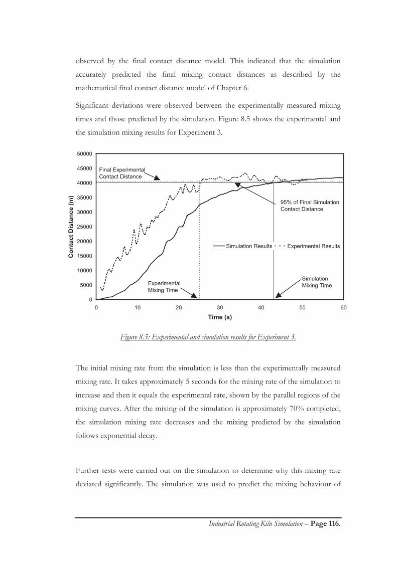
Industrial Rotating Kiln Simulation – Page 116.
observed by the final contact distance model. This indicated that the simulation
accurately predicted the final mixing contact distances as described by the
mathematical final contact distance model of Chapter 6.
Significant deviations were observed between the experimentally measured mixing
times and those predicted by the simulation. Figure 8.5 shows the experimental and
the simulation mixing results for Experiment 3.
0
5000
10000
15000
20000
25000
30000
35000
40000
45000
50000
0 10 20 30 40 50 60
Time (s)
Con
tact
Dis
tanc
e (m
)
Simulation Results Experimental Results
Final Experimental Contact Distance
95% of Final Simulation Contact Distance
Experimental Mixing Time
Simulation Mixing Time
Figure 8.5: Experimental and simulation results for Experiment 3.
The initial mixing rate from the simulation is less than the experimentally measured
mixing rate. It takes approximately 5 seconds for the mixing rate of the simulation to
increase and then it equals the experimental rate, shown by the parallel regions of the
mixing curves. After the mixing of the simulation is approximately 70% completed,
the simulation mixing rate decreases and the mixing predicted by the simulation
follows exponential decay.
Further tests were carried out on the simulation to determine why this mixing rate
deviated significantly. The simulation was used to predict the mixing behaviour of
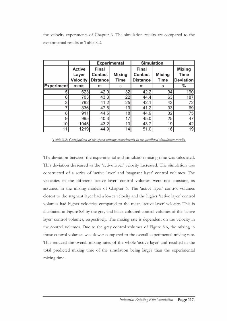
Industrial Rotating Kiln Simulation – Page 117.
the velocity experiments of Chapter 6. The simulation results are compared to the
experimental results in Table 8.2.
Active Layer
Velocity
Final Contact Distance
Mixing Time
Final Contact Distance
Mixing Time
Mixing Time
DeviationExperiment mm/s m s m s %
5 623 42.0 32 42.2 94 1906 703 43.8 22 44.4 63 1873 792 41.2 25 42.1 43 727 836 47.5 19 41.2 33 698 911 44.5 18 44.9 32 759 995 40.3 17 45.0 25 47
10 1045 43.2 13 43.7 19 4211 1219 44.9 14 51.0 16 19
Experimental Simulation
Table 8.2: Comparison of the speed mixing experiments to the predicted simulation results.
The deviation between the experimental and simulation mixing time was calculated.
This deviation decreased as the ‘active layer’ velocity increased. The simulation was
constructed of a series of ‘active layer’ and ‘stagnant layer’ control volumes. The
velocities in the different ‘active layer’ control volumes were not constant, as
assumed in the mixing models of Chapter 6. The ‘active layer’ control volumes
closest to the stagnant layer had a lower velocity and the higher ‘active layer’ control
volumes had higher velocities compared to the mean ‘active layer’ velocity. This is
illustrated in Figure 8.6 by the grey and black coloured control volumes of the ‘active
layer’ control volumes, respectively. The mixing rate is dependent on the velocity in
the control volumes. Due to the grey control volumes of Figure 8.6, the mixing in
those control volumes was slower compared to the overall experimental mixing rate.
This reduced the overall mixing rates of the whole ‘active layer’ and resulted in the
total predicted mixing time of the simulation being larger than the experimental
mixing time.

Industrial Rotating Kiln Simulation – Page 118.
Figure 8.6: ‘Active layer’ schematic illustrating the different velocity regions.
However, the deviation between the experimentally measured mixing time and the
mixing time predicted from the simulation was plotted against the mean ‘active layer’
velocity as shown in Figure 8.7. An inverse relationship is observed between the
deviation and the mean ‘active layer’ velocity. This relationship was not quantified
but illustrated that simulations conducted at higher ‘active layer’ velocities accurately
predicted the experimental behaviour of mixing in a rotating drum.
0
50
100
150
200
250
500 700 900 1100 1300 1500 1700 1900
Mean active layer velocity (mm/s)
Dev
iatio
n be
twee
n th
e pr
edic
ted
and
expe
rimen
tal m
ixin
g tim
es
Inverse relationship between deviation and mean active layer velocity
Figure 8.7: Deviation between the predicted and experimental mixing times as a function of the mean
‘active layer’ velocity.

Industrial Rotating Kiln Simulation – Page 119.
8.6.2 Segregation
As noted in Chapter 7, the dynamics of segregation could not be determined and
were assumed to be very fast in an industrial rotating kiln. In this section of the
thesis, the simulation behaviour of segregation was tested. Experiments were
conducted using the simulation model to determine the mean particle size in the
different layers of the bed, which in turn would reflect the amount of segregation.
The segregation model used only two layers and determined a proportion of material
in each layer with respect to the total proportion of that material in the bed. The
mean particle size could be calculated by multiplying the ratios of the materials with
the particle sizes of those materials and the overall proportion of that material in the
bed. The simulation used five layers and these layers were reduced to two for
comparison between the simulation and the experimental results. Layers 1, 2 and half
of 3 represented the outer layer and layers 4, 5 and the other half of layer 3
represented the inner layer. The experimental and simulation particle sizes are shown
in Table 8.3.
Experiment Inner Layer Outer Layer Inner Layer Outer Layer Inner Layer Outer Layermm mm mm mm % %
35 1.7 2.7 1.2 3.1 29.3 17.836a 3.2 4.3 2.6 4.1 20.8 5.436b 3.6 4.0 2.6 4.2 27.3 3.8
Average 25.8 9.0
Experimental Mean Diameter
Simulation Mean Diameter
Deviation between Simulation and
Table 8.3: Comparison of the mean particle size in the inner and outer layer for the experimental and
simulation segregation results.
The simulation predicted that more of the fine material accumulated in the inner
layer compared to the experimental results. This is illustrated by the larger particle
size differences in Table 8.3.
Industrial Rotating Kiln Simulation – Page 120.
Once again the lower mean ‘active layer’ velocities of the grey control volumes
account for this. According to the segregation model of Chapter 7, lower velocities
resulted in more material being segregated. The division of the ‘active layer’ into 22
individual ‘active layer’ control volumes resulted in the lower velocities, compared to
the mean ‘active layer’ velocity, in the grey control volumes of Figure 8.6. This
resulted in a decrease of the mixing rate but also resulted in additional segregation.
The segregation behaviour is expected to decrease with increased ‘active layer’
velocities, such as those encountered in industrial rotating kilns.
8.7 CHAPTER SUMMARY
A grid was developed that was suitable for the simulation of the mixing and segregation of solids in
the transverse section of a rotating drum. This grid consisted of two distinct zones, the ‘active layer’
and ‘stagnant layer’, each of which had differently functioning control volumes.
The simulation was tested against laboratory experiments and found to agree very well with the
prediction of the final amount of contact between two materials. Large deviations were observed
between the experimental mixing times and those observed from the simulation. These deviations
were inversely proportional to the mean ‘active layer’ velocity. The simulation could be used to
accurately predict the mixing behaviour at higher rotational velocities, such as those encountered in
industrial rotating kilns due to their larger drum diameter. Segregation differences were observed
between the experimental and segregation results. Once again these deviations were due to the
different velocities of the individual control volumes compared to the mean ‘active layer’ velocities. In
larger drums, the velocity of the ‘active layer’ increases and hence the segregation would decrease.

Industrial Rotating Kiln Simulation – Page 121.
CHAPTER 9
Simulation of the retort zone of the AOSTRA-Taciuk
Processor.
Two aims of this thesis were to derive a granular heat transfer model applicable to
the AOSTRA-Taciuk Processor and then to predict the behaviour of the retort zone
of the AOSTRA-Taciuk Processor. The simulation derived and confirmed in
Chapter 8 will be extended in this chapter to include the granular heat transfer
between the two materials and the thermal reactions of the materials in the
AOSTRA-Taciuk Processor so that the AOSTRA-Taciuk Processor can be
simulated.
9.1 DERIVATION OF THE GRANULAR HEAT TRANSFER
MODEL
As shown in Figure 2.8, there are various paths where heat is transferred to or from a
particle. These heat transfer mechanisms included conduction, convection and
radiation. The model developed here will focus on the heat transfer between the two
different materials that will be used in the AOSTRA-Taciuk Processor. The heat
transfer to the drum walls or from the gas phase above the bed to the bed of solids
will not be included in this model.
9.1.1 Granular heat transfer model assumptions
Due to the use of hard particles with minimum contact, conduction heat transfer
between the particles was assumed to be negligible (Molerus, 1997). Conduction into
the particle was assumed to be fast thus the heat transfer was limited to convection
or radiation to or from the surface of the particles.

Industrial Rotating Kiln Simulation – Page 122.
Natural convection was assumed to take place from the gases at the mean
temperature of the control volumes, which were described in Chapter 8, to the
individual particle types and temperatures in the control volumes. This convection
can results in heat transfer to or from the particles depending on the temperature
difference between the particles and the mean temperature of the control volume. It
was assumed that the gas phase, due to its lower heat capacity was at the mean
temperature of the solids in a control volume. It was also assumed that only natural
convection between the solid and the gas occurred because the velocities in the
control volumes were too low for forced convection to occur. The gas properties
required for the determination of the Nusselt number, as described below, were
evaluated at the mean gas temperature of each control volume.
Radiation was assumed to only take place from the hot material, the ash, to the cold
material, the preheated shale. Radiation to the drum and gas phase and vice versa was
not considered as this is beyond the scope of this simulation. The gases were
assumed to be non participating for the radiation heat transfer calculation.
Participating gases, such as H2O and CO2, would hinder the radiative heat transfer
through the gas phase.
The total heat transfer was assumed to be the addition of the natural convective heat
transfer and the radiative heat transfer.
The heat transfer process taking place in the kiln is unsteady heat transfer process,
however the heat transfer was assumed to be pseudo steady state so that the heat
transfer rate could be determined. This was justified by using small time steps in the
simulation and large temperature differences between the different materials
compared to the temperature changes of the materials in a time step. After
calculating (and balancing) the heat transfer rates, the new temperature of the
materials and the amount of volatile evolution occurring within that control volume
and time step were determined. These new temperatures were then used to
determine the heat transfer rate for the next time step.

Industrial Rotating Kiln Simulation – Page 123.
9.1.2 Natural convection heat transfer
To determine the natural convection heat transfer from the solid particles, the heat
transfer coefficient was calculated by using the Nusselt, LNu~ , number (Thomas,
1992):
kLhNuL~.~ (9.1)
where h is the heat transfer coefficient from the solid surface, L~ is the characteristic
length of the particle, which for a sphere is D/2 and k is the gaseous phase thermal
conductivity. LNu can be calculated using:
261~~ .331.0 LL RabaNu (9.2)
where a is 1.77 for spheres, b equals 278169Pr5.01
17.1 , LRa~ is the Rayleigh
number and Pr is the Prandtl number. LRa~ and LNu~ were determined for each
particle size and material type. The heat transfer coefficients will differ for different
particle sizes and temperature differences. The convective heat transfer rates to or
from the different material, Qc,i, were calculated using Equation 9.3:
imeaniiic TTAhQ , (9.3)
where the subscript i denotes the material type, Ai is the heat transfer area taken as
the total surface area for material i, Tmean was the mean gas temperature in the control
volume and Ti was the temperature of material i.
The heat transfer, qc,i, was then calculated for each material type and size using:
SAMPicic Qq .,, (9.4)
where SAMP is the time step or sampling time as determined in Chapter 8. Finally,
the total convective heat transfer from the ash was compared and balanced with the
total convective heat transfer to the shale. It was important to balance the total heat
transfer to ensure that the heating or cooling of the materials was realistic. The

Industrial Rotating Kiln Simulation – Page 124.
smallest total heat transfer magnitude was taken as the real total heat transfer and the
other heat transfer values were adjusted accordingly.
9.1.3 Radiation heat transfer
The radiation heat transfer was important due to the high temperatures and the large
particle sizes used in the AOSTRA-Taciuk Processor (Saatdjian & Large, 1988).
Radiation heat transfer occurred from the hot material, the ash, to the cold material,
the shale. The ash referred to in this chapter is the hot combusted spent shale
described in Chapter 1. The mean temperatures of the ash and shale were calculated.
The radiation heat transfer rates, Qr-SHALE, to the shale from the ash were determined
for each shale size, i, from the mean ash temperature, ASHT , as:
4,
4
,
,, .)( iSHALEASH
iSHALE
iSHALE
fRadiSHALEr TT
AA
ltlAQ (9.5)
where is the Stefan-Boltzmann constant, is the emmissivity of the solids, which
was taken to be representative of the emmissivity of soils of 0.90 (Thomas, 1992),
ARad is the area of radiation heat transfer, which was equal to the minimum of either
the total ash or the total shale surface area, fltl )( is the extent of mixing from Chapter
6, ASHALE,i is the surface area for the ith shale sample. iSHALET , is the mean
temperatures of the ith shale component in the control volume. The radiation heat
transfer rate from the ash was calculated by switching the ash and shale values in
Equation 9.5.
The total radiation heat transfer, qr,i, for each material, i, was calculated using:
SAMPirir Qq .,, (9.6)
The radiation heat transfer to the shale was compared and balanced with the
radiation heat transfer from the ash to ensure that the heat transfer was physically
realistic.

Industrial Rotating Kiln Simulation – Page 125.
9.1.4 Total heat transfer between the granular materials
Now the total heat transfer to or from a material in a control volume was taken as
the sum of the convective and radiative heat transfers. Thus:
irici qqq ,, (9.7)
However, the process being modelled was an unsteady state process and thus the
heat transfer resulted in changes to the temperatures of the materials. The heat
transfer needed to be re-evaluated at each time step due to changes in mixing,
segregation and material temperatures. This is considered in the next section.
The specific enthalpy of the material, )(tH , was calculated using:
i
iii
mtqtHtH )()1()( (9.8)
where )1(tHi is the specific enthalpy of the material prior to the heat transfer in
the latest time step, qi(t) is the heat transfer in the last time step, mi is the original
mass of that material type and size. The specific enthalpy was expressed per mass of
original material.
9.1.5 Calculation of the new material temperatures and the amount of volatile
evolution
In order to calculate the new temperatures of the materials and the amount of
volatile evolution, the thermal behaviour of the materials had to be known.
Berkovich (1999) studied the thermal behaviour of the Australian oil shales and ashes
and his models were used in this part of the thesis to complete the modelling of the
retort zone of the AOSTRA-Taciuk Processor. The enthalpy data was determined
for shale with the composition shown in Table 9.1. Only one shale type was tested
using the newly developed simulation.
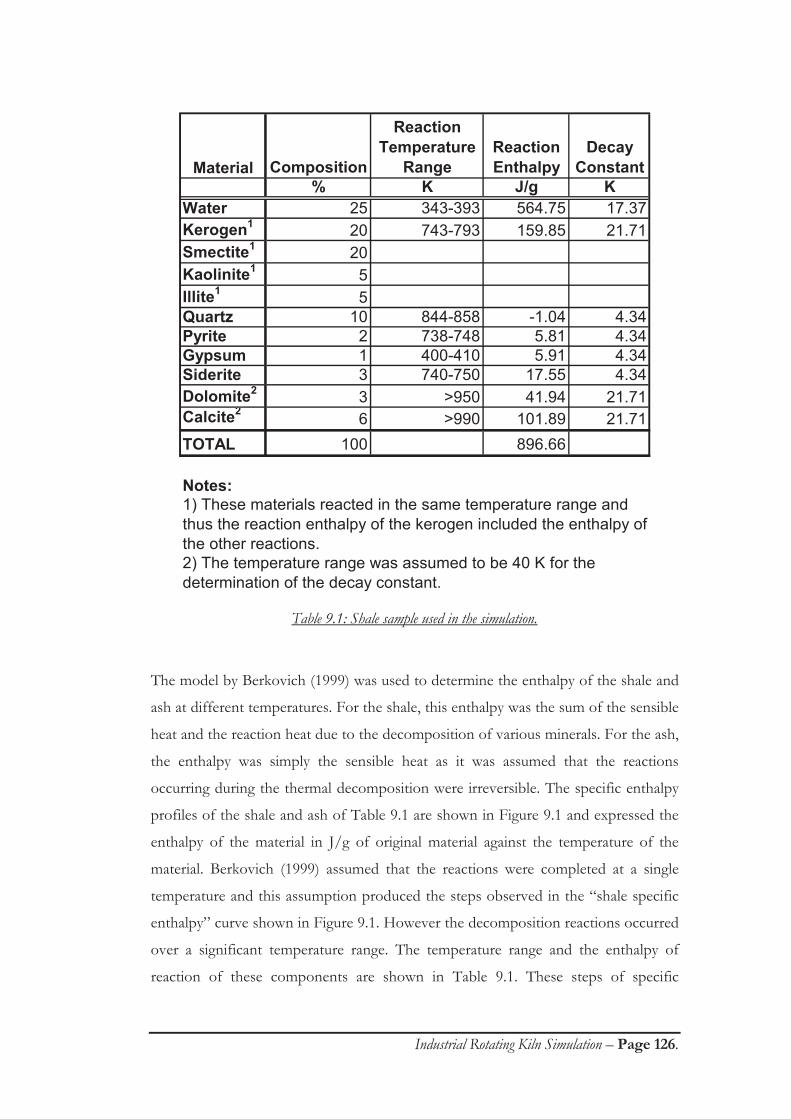
Industrial Rotating Kiln Simulation – Page 126.
Material Composition
Reaction Temperature
RangeReaction Enthalpy
Decay Constant
% K J/g KWater 25 343-393 564.75 17.37Kerogen1 20 743-793 159.85 21.71Smectite1 20Kaolinite1 5Illite1 5Quartz 10 844-858 -1.04 4.34Pyrite 2 738-748 5.81 4.34Gypsum 1 400-410 5.91 4.34Siderite 3 740-750 17.55 4.34Dolomite2 3 >950 41.94 21.71Calcite2 6 >990 101.89 21.71TOTAL 100 896.66
Notes:1) These materials reacted in the same temperature range and thus the reaction enthalpy of the kerogen included the enthalpy of the other reactions.2) The temperature range was assumed to be 40 K for the determination of the decay constant.
Table 9.1: Shale sample used in the simulation.
The model by Berkovich (1999) was used to determine the enthalpy of the shale and
ash at different temperatures. For the shale, this enthalpy was the sum of the sensible
heat and the reaction heat due to the decomposition of various minerals. For the ash,
the enthalpy was simply the sensible heat as it was assumed that the reactions
occurring during the thermal decomposition were irreversible. The specific enthalpy
profiles of the shale and ash of Table 9.1 are shown in Figure 9.1 and expressed the
enthalpy of the material in J/g of original material against the temperature of the
material. Berkovich (1999) assumed that the reactions were completed at a single
temperature and this assumption produced the steps observed in the “shale specific
enthalpy” curve shown in Figure 9.1. However the decomposition reactions occurred
over a significant temperature range. The temperature range and the enthalpy of
reaction of these components are shown in Table 9.1. These steps of specific

Industrial Rotating Kiln Simulation – Page 127.
enthalpy were larger than the changes in specific enthalpy occurring in a simulation
time step. The steps were thus approximated using exponential decay curves by
assuming that the reaction started at the lower temperature and was 90% completed
at the higher temperature of the temperature range shown in Table 9.1. Since the
enthalpy at all temperatures was expressed in J/original g of material, the heat
transfer was facilitated by allowing simple addition and subtraction of specific
enthalpies to the materials as shown in Equation 9.8.
0
200
400
600
800
1000
1200
1400
300 400 500 600 700 800 900 1000Temperature (K)
Spec
ific
Enth
alpy
(J/g
orig
inal
)
Ash specific enthalpy (J/g)
Shale specific enthalpy (J/g) -Berkovich (1999)Shale specific enthalpy (J/g) -MODEL
Figure 9.1: Enthalpy content of the shale and ash sample described in Table 9.1 (Berkovich, 1999).
The total enthalpy of the material was determined using the initial enthalpy of the
material and the heat transfer predicted by Equation 9.7. From this new enthalpy, the
temperature of the material can be found using the data from Figure 9.1. The total
volatile evolution can be determined using the new temperature and the thermo-
gravimetric analysis data shown in Figure 9.2.
Figure 9.2 is the mass loss curve, obtained from a thermo-gravimetric analysis of a
Stuart oil shale sample. The amount of mass lost can be evaluated at any temperature
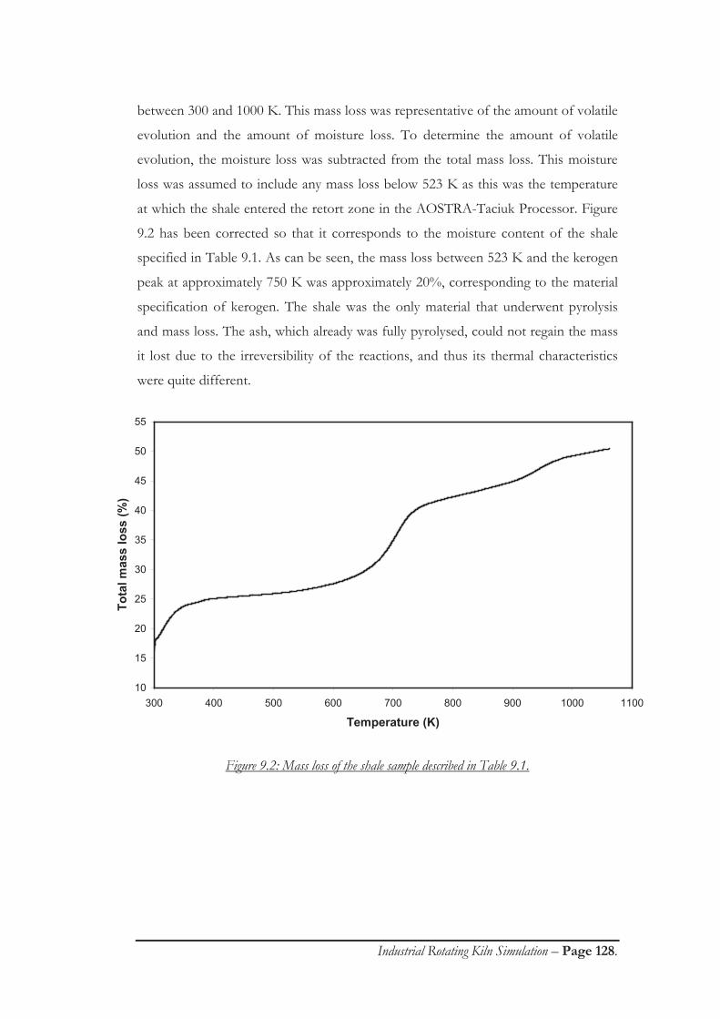
Industrial Rotating Kiln Simulation – Page 128.
between 300 and 1000 K. This mass loss was representative of the amount of volatile
evolution and the amount of moisture loss. To determine the amount of volatile
evolution, the moisture loss was subtracted from the total mass loss. This moisture
loss was assumed to include any mass loss below 523 K as this was the temperature
at which the shale entered the retort zone in the AOSTRA-Taciuk Processor. Figure
9.2 has been corrected so that it corresponds to the moisture content of the shale
specified in Table 9.1. As can be seen, the mass loss between 523 K and the kerogen
peak at approximately 750 K was approximately 20%, corresponding to the material
specification of kerogen. The shale was the only material that underwent pyrolysis
and mass loss. The ash, which already was fully pyrolysed, could not regain the mass
it lost due to the irreversibility of the reactions, and thus its thermal characteristics
were quite different.
10
15
20
25
30
35
40
45
50
55
300 400 500 600 700 800 900 1000 1100
Temperature (K)
Tota
l mas
s lo
ss (%
)
Figure 9.2: Mass loss of the shale sample described in Table 9.1.

Industrial Rotating Kiln Simulation – Page 129.
9.2 SIMULATION OF THE RETORT ZONE OF THE AOSTRA-
TACIUK PROCESSOR
In Chapter 8 a simulation model was developed for a rotating kiln and the mixing
and segregation mechanisms of this simulation were also validated. Deviations were
observed between the experimental and simulation results but it was shown that
increasing the drum size reduced these deviations. Increasing the drum size resulted
in faster mean active layer velocities, which reduced the deviation between the
experimentally measured and the simulation predicted mixing times. Increasing the
drum diameter also reduced the segregation effect.
The heat transfer mechanism described in section 9.1 was added to the simulation
and the dynamic behaviour of the retort zone of the AOSTRA-Taciuk Processor was
tested in this section of the thesis.
9.2.1 Material properties
The physical and chemical properties of the materials are shown in Table 9.1. Only
one sample of shale and ash was used to simplify the simulation. The simulation
could be extended to allow different material compositions to be used but that was
not within the scope of the research. The shale sample used to test the simulation is
representative of the Stuart oil shale deposit (Berkovich, 1999).
9.2.2 Case studies of the AOSTRA-Taciuk Processor operation
Industrial data for the AOSTRA-Taciuk Processor was not available and thus could
not be used for the validation of the simulation. To test the heat transfer model four
different operational variables were varied and the retort zone of the AOSTRA-
Taciuk Processor behaviour was studied. These variables were the mean particle size,
the initial temperature of the materials, the ratio of the materials and the rotational

Industrial Rotating Kiln Simulation – Page 130.
velocity of the drum. The different test cases are summarised in Table 9.2. The rate
of volatile evolution was calculated in each case and compared to the rate of volatile
evolution for the standard case, as shown in Case 2.
9.2.3 Results from Case 2
The results from Case 2 were compared to the results from the other simulation
tests. A detailed study was completed on Case 2 to test the performance of the
simulation.
Case number
Drum size Composition
Mean Size1
(Shale/Ash)
Initial Temperature (Shale/Ash)
Ratio (Shale:Ash)
Rotational Velocity
m mm/mm K/K - rpm1 6 As per Table 9.1 1.00/1.00 548/1048 0.32 52 6 As per Table 9.1 1.54/2.11 548/1048 0.32 53 6 As per Table 9.1 1.70/1.70 548/1048 0.32 54 6 As per Table 9.1 2.51/2.51 548/1048 0.32 55 6 As per Table 9.1 3.44/3.44 548/1048 0.32 56 6 As per Table 9.1 5.08/5.08 548/1048 0.32 57 6 As per Table 9.1 1.54/2.11 498/998 0.32 52 6 As per Table 9.1 1.54/2.11 548/1048 0.32 58 6 As per Table 9.1 1.54/2.11 598/1198 0.32 59 6 As per Table 9.1 1.54/2.11 548/1048 0.26 52 6 As per Table 9.1 1.54/2.11 548/1048 0.32 5
10 6 As per Table 9.1 1.54/2.11 548/1048 0.49 511 6 As per Table 9.1 1.54/2.11 548/1048 0.58 512 6 As per Table 9.1 1.54/2.11 548/1048 0.69 513 6 As per Table 9.1 1.54/2.11 548/1048 0.32 314 6 As per Table 9.1 1.54/2.11 548/1048 0.32 4
2 6 As per Table 9.1 1.54/2.11 548/1048 0.32 515 6 As per Table 9.1 1.54/2.11 548/1048 0.32 616 6 As per Table 9.1 1.54/2.11 548/1048 0.32 7
NOTES:
Material Properties
1) The shale and ash size specifications for the AOSTRA-Taciuk Processor were 1.54 mm and 2.11 mm respectively. These particle sizes were obtained using a mixture of the experimental particle sizes.
Table 9.2: Details of the case studies.

Industrial Rotating Kiln Simulation – Page 131.
9.2.3.1 Mixing and segregation of Case 2
The mixing of the bed in the AOSTRA-Taciuk Processor is shown in Figure 9.3.
This figure indicates that the mixing reached the maximum point of mixing after 39
seconds. The bed de-mixed itself after reaching this maximum. This was very unusual
and was not observed for the mixing tests of Chapter 8. A possible explanation for
this was due to the segregation of materials since multi-sized materials were used in
Case 2 and only a single sized particle ranges were used in the simulation experiments
of Chapter 8.
0
500
1000
1500
2000
2500
0 10 20 30 40 50 60 70 80 90 100Time (s)
Con
tact
Dis
tanc
e (m
)
Figure 9.3: Mixing dynamics of Case 2.
The mean particle sizes, after 220 seconds of simulation time, in the different
‘stagnant layer’ layers are shown in Figure 9.4. ‘Stagnant layer’ 1 was closest to the
wall and ‘stagnant layer’ 5 was closest to the rotational centre of the bed. As can be
seen, there was significant size segregation at this time. The mean ‘active layer’
velocity in Case 2 was 7.01 ms-1 and using the segregation model of Chapter 7,
segregation would not occur at this velocity. However velocities in some ‘active layer’
control volumes were less than the mean calculated velocity. The lowest velocity of

Industrial Rotating Kiln Simulation – Page 132.
1.60 ms-1 occurred in the grey ‘active layer’ control volumes of Figure 8.6 and these
low velocities allowed the materials to segregate.
0.0010
0.0012
0.0014
0.0016
0.0018
0.0020
0.0022
220 221 222 223 224 225 226 227 228 229 230
Time (sec)
Mea
n pa
rtic
le s
ize
(m)
Stagnant Layer 1 Stagnant Layer 2 Stagnant Layer 3Stagnant Layer 4 Stagnant Layer 5
Figure 9.4: Final segregated configuration of Case 2.
These results indicated that segregation is important in industrial rotating kilns. This
segregation would not be observed if the ‘active layer’ was considered as a single
entity, as it was in the experiments, rather than the 22 individual control volumes that
were used in the simulation. This is an advantage of using 22 single control volumes
to simulate the ‘active layer’ rather than one single entity.
9.2.3.2 Heat transfer, mean shale temperature and volatile evolution of Case 2
The important aspect of this part of the simulation was to test the heat transfer
model derived earlier in the chapter. Figure 9.5 shows the mixing extent and the
mean temperature of the shale. The mean shale temperature was closely linked to the
mixing extent of the material.
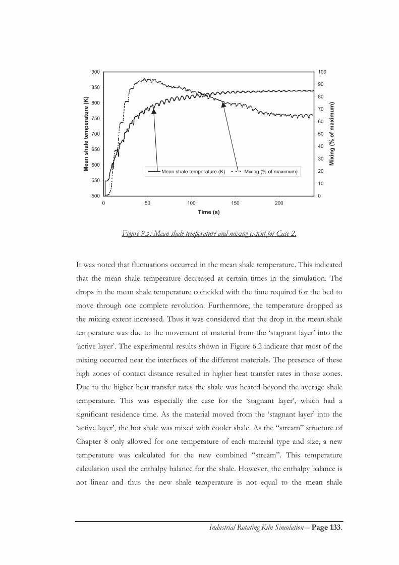
Industrial Rotating Kiln Simulation – Page 133.
500
550
600
650
700
750
800
850
900
0 50 100 150 200
Time (s)
Mea
n sh
ale
tem
pera
ture
(K)
0
10
20
30
40
50
60
70
80
90
100
Mix
ing
(% o
f max
imum
)
Mean shale temperature (K) Mixing (% of maximum)
Figure 9.5: Mean shale temperature and mixing extent for Case 2.
It was noted that fluctuations occurred in the mean shale temperature. This indicated
that the mean shale temperature decreased at certain times in the simulation. The
drops in the mean shale temperature coincided with the time required for the bed to
move through one complete revolution. Furthermore, the temperature dropped as
the mixing extent increased. Thus it was considered that the drop in the mean shale
temperature was due to the movement of material from the ‘stagnant layer’ into the
‘active layer’. The experimental results shown in Figure 6.2 indicate that most of the
mixing occurred near the interfaces of the different materials. The presence of these
high zones of contact distance resulted in higher heat transfer rates in those zones.
Due to the higher heat transfer rates the shale was heated beyond the average shale
temperature. This was especially the case for the ‘stagnant layer’, which had a
significant residence time. As the material moved from the ‘stagnant layer’ into the
‘active layer’, the hot shale was mixed with cooler shale. As the “stream” structure of
Chapter 8 only allowed for one temperature of each material type and size, a new
temperature was calculated for the new combined “stream”. This temperature
calculation used the enthalpy balance for the shale. However, the enthalpy balance is
not linear and thus the new shale temperature is not equal to the mean shale

Industrial Rotating Kiln Simulation – Page 134.
temperature of the different feeds. This non linearity caused the periodic fluctuations
observed in the mean shale temperature.
9.2.4 Results from the case studies
The case studies described in Table 9.2 were simulated and the volatile evolution was
calculated. In each case the dynamics of the volatile evolution was plotted in the
main chart of Figures 9.6 to 9.9. The inset in these figures represented the final
volatile evolution for each case.
9.2.4.1 Mean particle size effects
The mean particle size effect was tested from 1.00 mm to 5.08 mm. Case 2 had a
mean shale size of 1.54 mm and a mean ash size of 2.11 mm as described in Table
9.1. Cases 1, 3, 4, 5 & 6 had the same shale and ash particle sizes of 1.00, 1.70, 2.51,
3.44 and 5.08 mm respectively.
0
5
10
15
20
25
30
35
40
45
50
0 5 10 15 20 25 30 35 40 45 50
Time (sec).
Vola
tile
Evol
utio
n (%
age)
.
Case 1 Case 2 Case 3 Case 4 Case 5 Case 6
42.5
42.7
42.9
43.1
43.3
43.5
220 222 224 226 228 230
Figure 9.6: Simulation results for testing different mean particle sizes.

Industrial Rotating Kiln Simulation – Page 135.
The decrease in particle size ensured faster mixing as per the mixing mechanism of
Chapter 6. This was reflected in Figure 9.6 by faster evolution of volatiles. By using
smaller particle sizes the heat transfer occurred more rapidly because the rate of
particle heating was inversely proportional to the size of the particle. The final
volatile evolution results for the different particle sizes are shown in the inset of
Figure 9.6. It should be noted that all the cases, except for Case 2, reached the same
final state. This indicated that using a mixture of particle sizes compared to a single
particle size resulted in more volatiles being produced. This was due to the enthalpy
of the particles, as the enthalpy of particles was dependent on the size of the
particles. In Cases 1 and 3 to 6, the ratio of enthalpy of the shale to the ash was
identical as the same material size and ratios were used. However in Case 2 the
enthalpy of the ash was higher than the enthalpy of the shale due to the higher mean
particle size. This allowed more heat to be exchanged so that the shale reached a
higher temperature compared to the other cases. This higher temperature resulted in
a higher amount of final volatile evolution.
A further observation should be made regarding the fluctuations observed in Figure
9.6. The temperature fluctuations were described in the previous sections. The
volatile evolution is closely related to the temperature of the shale as shown in Figure
9.2. The periodic decreases in volatile evolution were due to the drop in the mean
shale temperature described above. Physically it would be impossible for the shale to
regain the volatiles that were evolved at a higher temperature and this was a
limitation of the “stream” structure. These fluctuations should be ignored and the
volatile evolution should be extrapolated across the troughs.
9.2.4.2 Initial temperature of the materials effects
Different initial temperatures of the materials were tested. It was expected that this
should strongly affect the heat transfer rate and the total amount of volatile
evolution. These results are shown in Figure 9.7.

Industrial Rotating Kiln Simulation – Page 136.
By increasing the initial temperatures of the shale and the ash the rate of volatile
evolution increased. This was due to the larger heat transfer rate, especially with
respect to the radiation heat transfer. The net result being that the final volatile
evolution also increased by increasing the initial temperatures.
0
5
10
15
20
25
30
35
40
45
50
0 5 10 15 20 25 30 35 40 45 50
Time (sec).
Vola
tile
Evol
utio
n (%
age)
.
Case 7 Case 2 Case 8
42.042.543.043.544.044.545.045.546.0
220 222 224 226 228 230
Figure 9.7: Simulation results for testing different initial material temperatures.
9.2.4.3 Ratio of the materials effects
Five different material ratios were considered. It was expected that decreasing the
shale to ash ratios should increase the mixing rate and thus the heat transfer. This
was reflected by the increased rate of volatile evolution with smaller shale to ash
ratios shown in Figure 9.8. As expected from an energy balance, increasing the ratio
of the shale to the ash reduced the final shale temperature and thus reduced the total
volatile evolution.

Industrial Rotating Kiln Simulation – Page 137.
0
5
10
15
20
25
30
35
40
45
50
0 5 10 15 20 25 30 35 40 45 50
Time (sec)
Vola
tile
Evol
utio
n (%
age)
Case 9 Case 2 Case 10 Case 11 Case 12
41.542.042.543.043.544.044.5
220 222 224 226 228 230
Figure 9.8: Simulation results for changes in the material ratio.
9.2.4.4 Rotational velocity effects
Changing the rotational velocity changed the mixing rate as shown in Chapter 6. The
effect of changing the rotational velocity on volatile evolution is shown in Figure 9.9.
Increasing the rotational velocity increased the rate of mixing and thus increased the
rate of volatile evolution. Figure 9.9 shows that the periodic fluctuations in the
volatile evolution discussed in section 9.2.4.1 were indeed dependent on the
rotational velocity since the period of fluctuations in Figure 9.9 corresponded to the
time of rotation of the material in the bed.
The rotational velocity also affected the final amount of volatile evolution. This is
unexpected in that the rotational velocity should not affect the final amount of
mixing, only the mixing rate.

Industrial Rotating Kiln Simulation – Page 138.
0
5
10
15
20
25
30
35
40
45
50
0 5 10 15 20 25 30 35 40 45 50
Time (sec)
Vola
tile
Evol
utio
n (%
age)
Case 13 Case 14 Case 2 Case 15 Case 16
42.6
42.8
43.0
43.2
43.4
43.6
220 222 224 226 228 230
Figure 9.9: Simulation results for different rotational velocities.
However, the final contact distance was measured and this final contact distance
increased when increasing the velocity. This arose due to the segregation of the
material, since multi-sized feeds were used in the simulation. The simulations carried
out at the lower velocities were more segregated compared to the results from the
simulation at the higher velocities. Since the shale and the ash had different mean
particle sizes, the segregation resulted in having more shale concentrated towards the
centre and the larger ash material towards the edge of the bed. The total heat transfer
was reduced because of this separation of the shale and the ash. The reduction in
heat transfer reduced the amount of volatile evolution.
9.3 LIMITATIONS OF THE SIMULATION
The cases studied in this chapter tested only a few possible parameters that may have
important implications on the behaviour of the retort section of the AOSTRA-
Taciuk Processor. The assumptions made in the heat transfer model must be noted

Industrial Rotating Kiln Simulation – Page 139.
before applying the model. Furthermore, the model was limited to a single type of oil
shale. The prediction of the volatile evolution only estimates the amount of volatiles
that will leave the AOSTRA-Taciuk Processor, it does not predict the quality of these
volatiles.
9.4 CHAPTER SUMMARY
In this chapter the simulation as derived in Chapter 8 was extended to include the granular heat
transfer between the preheated shale and the combusted spent shale in the AOSTRA-Taciuk
Processor.
The heat transfer model combined convective and radiative heat transfer mechanisms. The amount of
volatile evolution was calculated from the thermodynamic study of oil shales by Berkovich (1999)
and the developed granular heat transfer model.
Industrial data was not available to test the simulation so a case study was carried out to suggest
how the volatile evolution of the shale would be affected by changing certain operational parameters.
The case study suggested that the volatile evolution rate in the AOSTRA-Taciuk Processor could be
increased by reducing the particle size. It was found that the final amount of volatile evolution was
greater by using a multi-sized particle range compared to using a uniform particle size. Increasing the
initial temperatures of the materials resulted in a higher volatile evolution rate and a higher final
amount of volatile evolution. By reducing the ratio of shale to ash, the volatile evolution rate and the
final volatile evolution was also increased. However, it is not known whether the extra final volatile
evolution obtained was a desirable product or a byproduct from the mineral side reactions. Lastly,
increasing the rotational velocity increased the rate of volatile evolution due to the faster mixing rates
and also increased the final amount of volatile evolution.

Industrial Rotating Kiln Simulation – Page 140.
CHAPTER 10
Conclusions
Section 1.3 outlined the research objectives of this thesis. In line with the research
objectives, the conclusions of the current work are as follows:
1. The review of the rotating kiln literature showed that there is a lack of
quantitative models to predict the mixing and segregation of solids in
rotating drums. The models available only had limited applications and
could not be used to predict the behaviour of the AOSTRA-Taciuk
Processor, due to its unique nature. The need for new predictive models
was apparent.
2. Suitable experimental methods were developed, involving image analysis,
to measure the mixing and segregation behaviour in a laboratory sized
rotating drum. Further experiments were carried out to determine the
behaviour of the active layer since it was shown in the literature that the
active layer was important in the mixing, segregation and heat transfer in
a rotating kiln. The success of the mixing and segregation models was
attributed to the use of the active layer parameters. Studying the active
layer showed how the movement of material, which caused mixing and or
segregation was related to the drum size and scaling parameters were
developed with respect to the operational variables of rotating kilns.
3. A constant rate mixing mechanism was observed. However, on closer
analysis it was shown that mixing occurs through a series of steps
coinciding with the times when the materials entered the active layer.
This was physical proof that mixing only occurred in the active layer of a
rolling bed. The mixing of solids were modelled successfully with changes
in the following parameters: rotational velocity, particle size, drum
loading and material ratio. Complete mixing modelling required the
determination of both the mixing rate and the final contact distance
between the two materials being mixed. An active layer parameter was

Industrial Rotating Kiln Simulation – Page 141.
developed and a linear relationship was found to exist between this active
layer parameter and the mixing rate. Similarly a linear relationship was
observed between the final contact parameter and the final contact. The
mixing model was tested against independent experiments and accurately
predicted the mixing behaviour of mixing in different sized rotating
drums.
4. The segregation of solids in a rotating drum was successfully modelled
with changes in the active layer velocity and the particle size ratio of the
two materials. The segregation dynamics occurred too fast to be
modelled and it was assumed the segregation dynamics in large industrial
rotating kilns were negligible. The segregation model thus only
considered the final segregated configuration of the bed. The segregation
model was tested against independent experiments and accurately
predicted the final segregated configuration.
5. A simulation computer code was developed to simulate mixing and
segregation in a rotating drum. This simulation utilised the mixing and
segregation models derived in Chapters 6 and 7, respectively. It was
shown that the final amount of mixing was predicted accurately by the
simulation. However, the mixing dynamics and the final segregated
configuration were not predicted as accurately and this was due to the
lower velocities experienced in the control volumes of the grid compared
to the mean active layer velocity used in the modelling of the mixing
dynamics and the final segregated state. However, it was shown, that by
increasing the active layer velocity – due to increases in the drum
diameter or the rotational velocity - that the deviation between the
experimental results and those predicted by the simulation decreased.
This would indicate that the simulation could be used to predict the
mixing and segregation behaviour in industrial rotating kilns.
6. A heat transfer model was derived to determine the heat transfer between
granular materials in a bed of solids. This model included convective and
radiative heat transfer mechanisms and assumed that the heat transfer
was pseudo steady in order to determine the heat transfer rate. Previous

Industrial Rotating Kiln Simulation – Page 142.
work on the thermodynamic behaviour of oil shales was included in the
heat transfer model to allow realistic volatile evolution rates to be
predicted.
7. The simulation from Chapter 8 was extended to include the heat transfer
model. This allowed the retort section of AOSTRA-Taciuk Processor to
be simulated. The inclusion of typical thermal behaviour of oil shale
allowed the rate of volatile evolution to be predicted within the industrial
rotating kiln. Unfortunately this simulation could not be verified with
industrial data, as that information was not available. However, a case
study was carried out which tested operational variables available as part
of the simulation. Higher rates of volatile evolution were possible by
reducing the size of the material. Changing the material sizes did not
effect the total amount of volatiles evolved unless different material sizes
were used for the shale and ash. Increasing the initial material
temperatures or reducing the shale to ash ratio increased the rate of
volatile evolution and the final amount of volatiles. Lastly, increasing the
rotational velocity increased both the volatile evolution rate and the final
amount of volatiles.
8. The objectives of the research were achieved.

Industrial Rotating Kiln Simulation – Page 143.
Nomenclature
Symbol Units Notes
A - Dynamic computer array to store the image
information
A m² Particle surface area
AAL m² Transverse area of the stagnant layer
ABED m² Transverse area of the bed
Ai m² Convective heat transfer area for the ith fraction
ARad m² Radiative heat transfer area
ASHALE,i m² Surface area of the ith shale fraction
ASL m² Transverse area of the active layer
a - Experimental constant
b - Experimental constant
cc - Column of the image
C(x,t) Concentration at any position x and time t
D m Drum diameter
DiffD m²/s Diffusion coefficient
di m Mean particle size of the inner layer of the bed
do m Mean particle size of the outer layer of the bed
dp m Particle diameter
Fr - Froude number (ratio of centrifugal to gravitational
forces)
f - Mathematical function

Industrial Rotating Kiln Simulation – Page 144.
g m/s² Acceleration due to gravity
H - Height of the image in pixels
)(tHi J/g Enthalpy per unit original mass of the material at time t
h W/m².K Heat transfer coefficient
ih W/m².K Heat transfer coefficient for the ith ash or shale fraction
ij - Intercept for segregation model for layer j
ij( PSR) - Intercept for the segregation model for layer j as a
function of PSR
j - Layer index
k W/m.K Thermal conductivity of the material
0ek W/m.K Effective thermal conductivity of a stationary granular
medium
ek W/m.K Effective thermal conductivity of a moving granular
medium
tek W/m.K Effective thermal conductivity due to the flow of
material
L~ m Characteristic length, equals .dp/ 2 for spherical
particles.
L - Loading of the drum expressed as a percentage of the
drum volume
l(t) mm, m Contact at time t
l0 mm, m Initial contact
lf mm, m Final contact
M - Degree of mixing, equals zero for a non mixed system,
equals 1 for a fully mixed system, Rose (1959)
m - Index = 0.5

Industrial Rotating Kiln Simulation – Page 145.
mi g Original mass of the material
mj - gradient of segregation model for layer j
mj( PSR) - Gradient for the segregation model for layer i as a
function of PSR
N rpm Rotational velocity of the drum
LNu~ - Nusselt number
Pj - Proportion of segregated material in layer j
Po(t) - Order parameter for segregation, Cantelaude et al
(1997)
Pr - Prandtl number
PSR - Particle size ratio, large particle size divided by the
smaller particle size
Qc,i W Convective heat transfer rate to the ith ash or shale
fraction
Qr-SHALE,i W Radiative heat transfer rate to the ith shale fraction
qc,i J Convective heat transfer to the ith ash or shale fraction
qi J Total heat transfer to the ith ash or shale fraction
qr,i J Radiative heat transfer to the ith ash or shale fraction
R m Drum radius
RaL - Rayleigh number
RA m Distance from Apex A to the centre of rotation, Figure
5.1
RB m Distance from Apex B to the centre of rotation, Figure
5.1
r - Row of the image
Sn 1/s Segregation rate, Pollard & Henein (1989)

Industrial Rotating Kiln Simulation – Page 146.
ASHT K Average temperature of the ash
Ti K Temperature of material i
Tmean K Temperature of the gas phase in a control volume
TSHALE,i K Temperature of the ith shale fraction
t s Time
t1 s Mixing time for material 1, Woodle & Munro (1993)
t2 s Mixing time for material 2, Woodle & Munro (1993)
tm s Time required to fully mix the material in the bed.
U W/m².K Overall heat transfer coefficient to the particle
ALV m/s Mean active layer velocity
SLV m/s Mean stagnant layer velocity
W - Width of the image in pixels
x m Distance
X0 - X location of the centre of rotation
XA - X location of Apex A
XAL - Active layer proportion
Y0 - Y location of the centre of rotation
YA - Y location of Apex A
Q W Heat transfer to the particle
T K Temperature difference between the particle and its
surroundings
SL m².m/s Stagnant layer flux
mm/s,
m/s
Mixing rate
(t) mm/s, Mixing rate at time t

Industrial Rotating Kiln Simulation – Page 147.
m/s
- Segregation rate, Rose (1959)
A - Angle between Apex A and the centre of rotation
AB - Angle between Apex A and Apex B
- Angle from the centre of rotation to the pixel
- Emmissivity of the solids, taken to be 0.90
mm/s,
m/s
Active layer flux parameter
- Angle of inclination of the drum
- Material ratio
mm, m Final contact parameter
1 - Ratio of frictional coefficient for material 1, Woodle &
Munro (1993)
2 - Ratio of frictional coefficient for material 2, Woodle &
Munro (1993)
42 ./ KmW
Stefan Boltzmann constant
s time constant characterising kinetics of segregation
min s Minimum residence time
SAMP s Sampling time, time step
SLCV,res s Residence time of the stagnant layer control volumes
rad/s Rotational velocity of the drum
c rad/s Critical rotational velocity of the drum

Industrial Rotating Kiln Simulation – Page 148.
References
Alonso, M., Satoh, M., Miyanami, K., “Optimum combination of size ratio, density ratio and
concentration to minimize free surface segregation”, Powder Technol., 68, 145-152
(1991).
Arpaci, V., “Conduction Heat Transfer”, Addison Wesley, London (1966).
Australian Institute of Petroleum, “Queensland oil shale plans may bring Australian
petroleum industry back to its roots”, Petroleum Gazette, 28, 3-10 (1993).
Baker, C., G., “Air-solids drag in cascading rotary dryers”, Drying Technol., 10, 365-393
(1992).
Barker, J., J., “Heat transfer in packed beds”, Ind. Eng. Chem., 57, 43-51 (1965).
Barr, P., Brimacombe, J., Watkinson, A., “A heat transfer model for the rotary kiln: Part 1.
Pilot Kiln Trials”, Metall. Trans. B, 20B, 391-402 (1989a).
Barr, P., Brimacombe, J., Watkinson, A., “A heat transfer model for the rotary kiln: Part 2.
Development of the Cross Section Model”, Metall. Trans. B, 20B, 403-419 (1989b).
Berkovich, A., J., Young, B., R., Levy, J., H., Schmidt, J., S., “Thermal characteristics of
Australian oil shales”, J. Therm. Anal., 49, 737-743 (1997).
Berkovich, A., J., “The thermal characterisation of Australian tertiary oil shales”, Ph.D.
Dissertation, University of Technology, Sydney, New South Wales, Australia
(1999).
Boateng, A., A., “Rotary kiln transport phenomena”, Ph.D. Dissertation, University of
British Columbia, British Columbia, Canada (1993).
Boateng, A., Barr, P., “A thermal model for the rotary kiln including heat transfer within the
bed”, Int. J. Heat Mass Transfer, 39, 2131-2147 (1996).
Boateng, A., Barr, P., “Modelling of particle mixing and segregation in the transverse plane of the
rotary kiln”, Chem. Eng. Sci., 51, 4167-4181 (1996).
Boateng, A., Barr, P., “Granular flow behaviour in the transverse plane of a partially filled
rotating cylinder”, J. Fluid Mech., 330, 233-249 (1997).
Bram, L., “Whatever happened to the Rundle Twins?”, Aust. Mining, 87, 52-58 (1995).
Bridgewater, J., “Fundamental powder mixing mechanisms”, Powder Technol., 15, 215-236
(1976).

Industrial Rotating Kiln Simulation – Page 149.
Cahn, D., S., Fuerstenau, D., W., “Simulation of diffusional mixing of particulate solids by
Monte Carlo techniques”, Powder Technol., 1, 174-182 (1967).
Cantelaube, F., Bideau, D., Roux, S., “Kinetics of segregation of granular media in a two-
dimensional rotating drum”, Powder Technol., 93, 1-11 (1997).
Charlip, David, “The BMP file format, Part 1”, Dr. Dobb's J., 20, 44-49 (1995a).
Charlip, David, “The BMP file format, Part 2”, Dr. Dobb's J., 20, 34-42 (1995b).
Clément, E., Rajchenbach, J., Duran, J., “Mixing of a granular material in a bidimensional
rotating drum”, Europhys. Lett., 30, 7-12 (1995).
Dixon, A., Cresswell, D., “Theoretical prediction of effective heat transfer parameters in packed
beds”, AIChE J., 25, 663-676 (1979).
Donald, M., B., Roseman, B., “Mechanisms in a horizontal drum mixer”, Br. Chem. Eng.,
7, 749-753 (1962).
Ferron, J., Singh, D., “Rotary kiln transport processes”, AIChE J., 37, 747-758 (1991).
Gurgel, J., M., Kluppel, R., “Thermal conductivity of hydrated silica-gel”, The Chem. Eng.
J., 61, 133-138 (1996).
Henein, H., Brimacombe, J., K., Watkinson, A., P., “The modelling of transverse solids
motion in rotary kilns”, Metall. Trans. B, 14B, 207-220 (1983a).
Henein, H., Brimacombe, J., K., Watkinson, A., P., “Experimental study of transverse bed
motion in rotary kilns”, Metall. Trans. B, 14B, 191-205 (1983b).
Henein, H., Brimacombe, J., K., Watkinson, A., P., “An experimental study of segregation
in rotary kilns”, Metall. Trans. B, 16B, 763-774 (1985).
Hogg, R., Cahn, D., S., Healy, T., W., Fuerstenau, D., W., “Diffusional mixing in an ideal
system”, Chem. Eng. Sci., 21, 1025-1038 (1966).
Hogg, R., Fuerstenau, D., W., “Transverse mixing in rotating cylinders”, Powder Technol.,
6, 139-148 (1972).
Hogg, R., Shoji, K., Austin, L., “Axial transport of dry powders in horizontal rotating
cylinders”, Powder Technol., 9, 99-106 (1974).
Hunt, M., L., “Discrete element simulations for granular material flows: effective thermal
conductivity and self-diffusivity”, Int. J. Heat Mass Transfer, 40, 3059-3068 (1997).
Kelbert, F., Royere, C., “Lateral mixing and heat transfer in a rolling bed”, Int. Chem.
Eng., 31, 441-449 (1991).
Kohring, G., A., “Studies of diffusional mixing in rotating drums via computer simulations”, J.
Phys, 5, 1551-1561 (1995).

Industrial Rotating Kiln Simulation – Page 150.
Kramers, H., Croockewit, P., “The passage of granular solids through inclined rotary kilns”,
Chem. Eng. Sci., 1, 259-265 (1952).
Kunii, D., Smith, J., M., “Heat transfer characterictics of porous rocks”, AIChE J., 6, 71-77
(1960).
Lebas, E., Hanrot, F., Ablitzer, D., Houzelot, J., L., “Experimental study of residence time,
particle movement and bed depth profile in rotary kilns”, Can. J. Chem. Eng., 73, 173-
180 (1995).
Leger, C., B., Cook, C., A., Cundy, V., A., Sterling, A., M., Deng, X., Lighty, J., S.,
“Bed mixing and heat transfer in a batch loaded rotary kiln”, Environ. Prog., 12, 101-
109 (1993).
Lehmberg, J., Hehl, M., Schugerl, K., “Transverse mixing and heat tarnsfer in horizontal
rotary drum reactors”, Powder Technol., 18, 149-163 (1977).
Levine, John, “Programming for graphics files in C and C++”, John Wiley & Sons,
Brisbane, Australia (1994).
Luse, Marv, “The BMP file format”, Dr. Dobb's J., 19, 18-22 & 82-85 (1994).
Molerus, O., “Heat transfer in moving beds with a stagnant interstitial gas”, Int. J. Heat Mass
Transfer, 40, 4151-4159 (1997).
Mu, J., Perlmutter, D., D., “The mixing of granular solids in a rotary cylinder”, AIChE J.,
26, 928-934 (1980).
Nakagawa, M., Caprihin, A., Fukushima, E., “MRI of granular flows in a rotating cylinder”
in Cavitation and Multiphase Flow Forum, 135, 23-27, ASME, Los Angeles,
CA, USA (1992).
Nityanand, N., Manley, B., Henein, H., “An analysis of radial segregation for different sized
spherical solids in rotary cylinders”, Metall. Trans. B, 17B, 247-257 (1986).
Papadakis, S., E., Langrish, T., A., Kemp, I., C., Bahu, R., E., “Scale-up of cascading
rotary dryers”, Drying Technol., 12, 259-277 (1994).
Perron, J., Bui, R., “Rotary cylinders: solid transport prediction by dimensional and rheological
analysis”, Can. J. Chem. Eng., 68, 61-68 (1990).
Pershin, V., F., “Modelling of loose material mixing process in the cross section of a rotary drum”,
Theor. Found. Chem. Eng., 20, 324-328 (1987).
Pershin, V., F., Mineav, G., A., “Energetic approach in determination of motion of a granular
material in a rotating drum”, Theor. Found. Chem. Eng., 23, 432-435 (1989a).
Industrial Rotating Kiln Simulation – Page 151.
Pershin, V., F., Mineav, G., A., “Modelling the mixing of a granular material in a cross section
of a smooth rotating drum”, Theor. Found. Chem. Eng., 23, 249-255 (1989b).
Pickering, R., W., Feakes, F., Fitzgerald, M., “Time for passage of material through rotary
kilns”, J. Appl. Chem., 1, 13-19 (1951).
Pollard, B., L., Henein, H., “Kinetics of radial segregation of different sized irregular particles in
rotary cylinders”, Can. Metall. Quart., 28, 29-40 (1989).
Raghavan, G., S., V. Harper, J., M., Haberstroh, R., D., “Heat transfer using granular
media”, Trans. ASAE, 589-592 (1974).
Rao, S., M., Toor, H., L., “Heat transfer between particles in packed beds”, Ind. Eng. Chem.
Fundam., 23, 294-298 (1984).
Rao, S., M., Toor, H., L., “Heat transfer from a particle to a surrounding bed of particles. Effect
of size and conductivity ratios”, Ind. Eng. Chem. Res., 26, 469-474 (1987).
Ray, A., K., Prasad, K., K., Ray, H., S., Sen, P., K., “Residence time in a rotary kiln for
sponge iron making- prediction from kinetic data”, Steel India, 17, 16-20 (1994).
Ristow, G., H., “Particle mass segregation in a two-dimensional rotating drum”, Europhys.
Letters, 28, 97-101 (1994).
Rose, H., E., “A suggested equation relating to the mixing of powders and its application to the
study of the performance of certain types of machine”, Trans. Inst. Chem. Eng., 37, 47-
64 (1959).
Roseman, B., Donald, M., B., “Effects of varying the operating conditions of a horizontal drum
mixer”, Br. Chem. Eng., 7, 823-827 (1962).
Rutgers, R., “Longitudinal mixing of granular material flowing through a rotating cylinder. Part I
Descriptive and theory”, Chem. Eng. Sci., 20, 1079-1087 (1965a).
Rutgers, R., “Longitudinal mixing of granular material flowing through a rotating cylinder. Part
II Experimental”, Chem. Eng. Sci., 20, 1089-1100 (1965b).
Saatdjian, E., Large, J., F., “Heat transfer in a countercurrent gas-solid, packed column”, J.
Heat Transfer., 110, 385-389 (1988).
Saeman, W., C., “Passage of solids through rotary kilns”, Chem. Eng. Prog., 47, 508-514
(1951).
Sai, P., S., T., Surender, G., D., Damodaran, A., D., Suresh, V., Philip, Z., G.,
Sankaran, K., “Residence time distribution and material flow studies in a rotary kiln”,
Metall. Trans. B, 21B, 1005-1011 (1990).
Schotte, W., “Thermal conductivity of packed beds”, AIChE J., 6, 63-67 (1960).
Industrial Rotating Kiln Simulation – Page 152.
Sherritt, R., G., Caple, R., Behie, L., Mehrotra, A., “The movement of solids through flighted
rotating drums. Part 1: Model Formulation”, Can. J. Chem. Eng., 71, 337-346
(1993).
Sherritt, R., G., Caple, R., Behie, L., Mehrotra, A., “The movement of solids interaction
through flighted rotating drums. Part 2: Solids-Gas Inetraction and Model Validation”,
Can. J. Chem. Eng., 72, 240-248 (1994).
Sotocinal, S., A., Alikhani, Z., Raghavan, G., S., V., “Heating/ drying using particulate
medium: a review. Part 1. General and heat transfer parameters”, Drying Technol., 15,
441-459 (1997a).
Sotocinal, S., A., Alikhani, Z., Raghavan, G., S., V., “Heating/ drying using particulate
medium: a review. Part 2. Equipment”, Drying Technol., 15, 461-475 (1997b).
Southern Pacific Petroleum Financial report, Southern Pacific Petroleum N.L., 1991.
Sullivan, W., N., Sabersky, R., H., “Heat transfer to flowing granular media”, Int. J. Heat
Mass Transfer, 18, 97-107 (1975).
Sze, M., W., Ang, H., M., Tade, M., O., “Particle dynamics in a cold model rotary kiln” in
Proc of the 23rd Aust. Chem. Eng. Conf., 4, 27-32, IEAust, Adelaide, SA,
Australia (1995).
Taciuk, W., Turner, R., “Development status of Australian oil shale processing utilizing the
Taciuk processor”, Fuel, 67, 1405-1407 (1988).
Tackie, E., Watkinson, A., Brimacombe, J., “Experimental study of the elutriation of
particles from rotary kilns”, Can. J. Chem. Eng., 67, 806-817 (1989).
Tackie, E., Watkinson, A., Brimacombe, J., “Mathematical modelling of the elutriation of
fine materials from rotary kilns”, Can. J. Chem. Eng., 68, 51-60 (1990).
Thomas, L., C., “Heat Transfer”, Prentice Hall, New Jersey (1992).
Wes, G., W. ,J., Drinkenburg, A., A., H., Stemerding, S., “Solids mixing and residence
time distribution in a horizontal rotary drum reactor”, Powder Technol., 13, 177-184
(1976a).
Wes, G., W. ,J., Drinkenburg, A., A., H., Stemerding, S., “Heat transfer in a horizontal
rotary drum reactor”, Powder Technol., 13, 185-192 (1976b).
Williams, J., Khan, M., “The mixing and segregation of particulate solids of different particle
size”, Chem. Eng., 269, 19-25 (1973).
Woodle, G., Munro, J., “Particle mixing and mixing in a rotary kiln”, Powder Technol.,
76, 241-245 (1993).

Industrial Rotating Kiln Simulation – Page 153.
Yagi, S., Kunii, D., “Studies on effective thermal conductivities in packed beds”, AIChE J., 3,
373-381 (1957).
Yang, L., Farouk, B., “Modelling of solid particle flow and heat transfer in rotary kiln calciners”,
J. Air Waste Manage. Assoc., 47, 1189 – 1196 (1997).
Zik, O., Stavans, J., “Self-diffusion in granular flows”, Europhys. Letters, 16, 255-258
(1991).
Zingarelli, J., Muradian, A., Stephenson, L., “Upgrading of Stuart oil shale”, Fuel, 67,
1408-1410 (1988).
Industrial Rotating Kiln Simulation – Page 154.
APPENDICES
Appendix 1: The bitmap file format.
The Bitmap file format is a type of a computer graphics file. Bitmaps are the most
commonly used graphics files since they represent a picture as a rectangular array of
dots (Levine, 1994). Luse (1994) and Charlap (1995a, b) studied the bitmap file
format and published papers on the structure of a bitmap file.
To the untrained eye, a Bitmap file just consists of a series of hexadecimal values.
However, there is a structure to the Bitmap file format. In short a bitmap file
consists of a File Header, a Bitmap Header, an optional Colour Palette and a Bitmap.
Figure A1.1 shows a typical bitmap file viewed as text. Figure A1.2 shows the image
represented by the bitmap file of Figure A1.1. The values of Figure A1.1 have been
allocated different type faces to represent the different sections of the bitmap file.
These will be discussed in more detail in this appendix.
Each entry, consisting of two values from 0 to F, of Figure A1.1 represent 8 bits or 1
byte of information. A WORD consists of 32 bits or 4 bytes of information.
A1.1 STRUCTURE OF THE BITMAP FILE
Bitmaps can exist with different numbers of colours, from a monochrome bitmap,
where each pixel is represented by 1 bit, to a full colour bitmap, where each pixel is
represented by 32 bits. In the current research, 256 colour bitmap files were used and
the structure of this type of bitmap is the focus of this appendix.

Industrial Rotating Kiln Simulation – Page 155.
42 4D AE 04 00 00 00 00 00 00 36 04 00 00 28 00
00 00 0A 00 00 00 0A 00 00 00 01 00 08 00 00 00
00 00 78 00 00 00 00 00 00 00 00 00 00 00 00 00
00 00 00 00 00 00 00 00 00 00 40 00 00 00 80 00
00 00 FF 00 00 00 00 20 00 00 40 20 00 00 80 20
00 00 FF 20 00 00 00 40 00 00 40 40 00 00 80 40
00 00 FF 40 00 00 00 60 00 00 40 60 00 00 80 60
…… ……
FF 00 FF 80 FF 00 00 A0 FF 00 40 A0 FF 00 80 A0
FF 00 FF A0 FF 00 00 C0 FF 00 40 C0 FF 00 80 C0
FF 00 FF C0 FF 00 00 FF FF 00 40 FF FF 00 80 FF
FF 00 FF FF FF 00 00 FF FF FF FF FF FF FF FF E0
00 00 FF 00 FF FF FF FF FF FF 00 FF 00 00 FF FF
….. ….
FF E0 FF FF 00 00 FF E0 FF FF FF FF FF FF E0 FF
00 00 00 FF FF FF FF FF FF FF FF E0 00 00
Figure A1.1: Text display of a 256 colour bitmap file.
A1.1.1 File Header
The File Header is shown as the BOLD font in Figure A1.1. The first two bytes of
any image file indicates the image format. In the case of a bitmap file, the first two
entries are 42 and 4D, respectively. This represents the characters B and M, short for
BitMap. This is followed by a WORD to represent the size of the image, which by
default should represent the size in bytes but was often set to zero or could contain
the size of the file in words instead of bytes (Luse, 1994). The co-ordinates of the
image hotspot is located in the next WORD. The hotspot is only used when the
image in the file is used as a cursor. The final WORD of the File Header represents
the offset from the beginning of the file to the beginning of the bitmap. This is
important if different image formats are used since the size of the colour palette

Industrial Rotating Kiln Simulation – Page 156.
depends on the number of colours in the palette. The File Header consists of 14
bytes of data.
A1.1.2 Bitmap Header
The Bitmap Header is shown as the STRIKETHROUGH font in Figure A1.1. The
first WORD in the Bitmap Header is the size in bytes of the Bitmap Header. This
value is also used to indicate what version of a bitmap file is being worked with. The
second and third WORDs in the Bitmap Header contain the width and height of the
image in pixels, respectively. The Bitmap Header also contains data to determine the
number of bit planes used, the number of bits used per pixel, whether compression
has been used and if so what type of compression and finally the size of the Bitmap
in bytes. The Bitmap Header is 40 bytes in length.
A1.1.3 Colour Palette
The colour palette is shown as the ITALIC font in Figure A1.1. For a 256 colour
bitmap, the Colour Palette consists of 256 combination of the Red, Green and Blue
values to represent the colours in the image. Each colour is buffered to a WORD so
the total size of the Colour Palette is 1024 bytes.
A custom colour palette was created for the analysis of the images obtained from the
experiments. This palette consisted of a 100 colour specifications representing the
black material, 100 colour specifications representing the orange material and 50
colour specifications representing the background colour (white) of the drum. Six
other colours were required to complete the 256 colour palette. These 6 colours were
different shades of red, green and blue and were used to represent important points
in the images such as the apex positions, as shown in Figures 5.1 and 5.2.

Industrial Rotating Kiln Simulation – Page 157.
The colour palette used in Figure A1.1 is the Windows default colour palette. The
first colour specification equals 00 00 00 00. This represents values of 0 for the blue,
green and red, respectively. The last 00 is used to buffer the colour to a WORD. This
colour specification is referred to as colour 00 in the Bitmap.
LEGENDWhite pixelRed pixelBlack pixel
Figure A1.2: Image represented by data of Figure A1.1.
A1.1.4 Bitmap
The data representing the pixels is represented by the UNDERLINED values in
Figure A1.1. This data follows immediately after the Colour Palette. The image is
stored as a series of pixels from the bottom up. Each pixel in the line is represented
by the index of the colour from the Colour Palette. Each line of data is buffered to
the next full WORD. For example, if the current image has a width of 10 pixels, each
pixel is represented by a value from 0 to 255 to represent the pixels colour from the
Colour Palette. However, a WORD contains 4 bytes so 3 WORDs are required to
represent the line in the image. The values of these last two bytes of the last WORD
are set equal to 00.

Industrial Rotating Kiln Simulation – Page 158.
A1.2 READING THE BITMAP FILE
In order to read the data in a bitmap, the format of the file as described above must
be known. Since a bitmap file consists of hexadecimal values, some of which are
unprintable, it is necessary to open the file as a binary file if it is desired to analyse
them. This allowed all the data in the file to be analysed. Since all the experimental
images were similar in format only the width and height of the images needed to be
read from the file. These fields consisted of a WORD. Figure A1.2 represents a
bitmap image of 10 pixels wide and 10 pixels high. This is expressed in the Bitmap
Header by the values 0A 00 00 00. This hexadecimal value equals 10 in decimal. The
images used in the experiments were all calibrated to the custom Colour Palette
described above. The Colour Palette from the images was thus known and did not
need to be read. The bytes of the Bitmap were read, the value indicating what colour
the pixel represented from the colour table.
For example looking at the first entry of the Bitmap of Figure A1.1: this byte has the
value of 00, which has a decimal value of 0. Thus the first pixel represents the zeroth
colour in the colour table which was black. Thus the first pixel (from the bottom up)
of the image is a black pixel. This is shown in Figure A1.2. Continuing along, there
are 8 values of FF, representing the white colour followed by 1 value of E0, which
represents the 225th colour in the Colour Palette and is the red colour. Figure A1.2
was drawn using the default Windows colour palette. In the experimental images the
1st to the 100th entries in the Colour Palette represented the black material, the
second hundred represented the orange material and the next 50 colour
specifications represented the white colour of the drum. This was followed by 2
green, 2 blue and 2 red colour specifications.
The psuedocodes for the programs that converts bitmap files into data that can be
analysed are given in Appendix 2.

Industrial Rotating Kiln Simulation – Page 159.
Appendix 2: Psuedo codes for the software written as part
of the thesis.
A2.1 CONVERTING THE BITMAP IMAGES TO AN ARRAY
1. Obtain file name from user input.
2. Open the file in binary mode to allow non printable characters to be read as hexadecimal values.
3. Read bytes 19 to 22 to determine the width, W, of the image.
4. Read the next WORD (bytes 23 to 26) to obtain the height, H, of the image.
5. Skip the next 28 bytes. The 29th byte is the start of the Colour Palette.
5.1. If details of the colour specifications are required, create an array so that the data can be read.
5.2. If details of the colour specification are not required (as is the case in the current image analysis work – since the colour specifications are known), skip the 1024 bytes of the Colour Palette.
6. Create a dynamic array, Ä, of W+ 2 columns and H+ 2 rows.
7. Allocate the values in the 1st column, the (W+ 2)nd, the first row and the (H+ 2)nd row of Ä to the buffer value, which in this case was taken as 9.
8. Read the data from the Bitmap part of the image into the array:
8.1. Loop through the rows, index rr starting at 2 since first row is the buffer,
8.1.1.Loop through the columns, index c starting at 2,
8.1.1.1. Read the next byte (pixel), P, from the Bitmap.
8.1.1.2. If the value of P is between 0 & 99, Ä[ r, c]= 0 (black).
8.1.1.3. If the value of P is between 100 & 199, Ä[ r, c]= 1 (orange).
8.1.1.4. If the value of P is between 200 & 249, Ä[ r, c]= 2 (white).
8.1.1.5. If the value of P is either 250 or 251, Ä[ r, c]= 4 (green).
8.1.1.6. If the value of P is either 252 or 253, Ä[ r, c]= 5 (blue).
8.1.1.7. If the value of P is either 254 or 255, Ä[ r, c]= 6 (red).
8.1.1.8. Increase c by one.
8.1.2.Increase r by one.
9. Close the bitmap file.
10. Analyse Array using either the mixing or segregation routing.
11. If not destroyed, destroy dynamic array, Ä.
if cc
<=
W+
1 if
rr <=
H+
1

Industrial Rotating Kiln Simulation – Page 160.
A2.2 PSUEDO CODE FOR THE MIXING ANALYSIS
1. Obtain experimental series name and numbers from user input.
2. Create the results file.
3. Loop through image series starting at the first image.
3.1. Set mixing contact equal to zero.
3.2. Read Bitmap into dynamically allocated array, as described above.
3.3. Loop through the rows, rr, of the array starting at 2.
3.3.1.Loop through the columns, c, of the array starting at 2 & read pixel value, P.
3.3.1.1. If P equals 1, check surrounding pixels.
3.3.1.1.1. Check P[ r± 1, c] and P[ r, c± 1].
3.3.1.1.1.1. If surrounding pixel is of type 0 increase contact by 1.
3.3.1.2. Increase c by 1.
3.3.2.Increase r by 1.
3.4. Write total contact, in pixels length, between Orange and Black of current image to file.
3.5. Delete dynamically allocated array.
3.6. Increase image number.
4. Save results file.
A2.3 PSUEDO CODE FOR THE SEGREGATION ANALYSIS
1. Obtain experimental series name and numbers from user input.
2. Create the bed outline file.
3. Read bitmap of the outline described in Chapter 7 into a dynamically allocated array.
3.1. Loop through the outline image and find the location of the green pixels. This shows the position of Apex A and Apex B.
3.2. Calculate the position of the rotational centre of the bed from Apex A and Apex B as described in Chapter 5.
3.3. Loop through the pixels of the outline image,
3.3.1.If the current pixel, P, is white,
if cc
<=
W+
1
if rr <
= H
+1
if im
age n
umbe
r <=
total
num
ber o
f ima
ges

Industrial Rotating Kiln Simulation – Page 161.
3.3.1.1. Check surrounding pixels for black pixels, if a black pixel is found calculate the distance and angle from the centre of rotation to P.
3.3.1.2. Save the distance and angle.
3.4. Sort and reduce array from approximately 9000 points to 360 points, one for each degree of the circumference at the centre of rotation.
3.5. Close bitmap.
3.6. Save the data in the bed outline file.
4. Create a segregation results file.
5. Loop through segregation images.
5.1. Read segregation image into a dynamically allocated array.
5.1.1.Loop through the segregation image and find the location of the green pixels. This shows the position of Apex A and Apex B.
5.1.2.Calculate the position of the rotational centre of the bed from Apex A and Apex B as described in Chapter 5.
5.1.3.Loop through the pixels of the segregation image,
5.1.3.1. If the current pixel, P, is orange or black,
5.1.3.1.1. Determine the distance, DP-O from P to the centre of rotation.
5.1.3.1.2. Determine the angle, , from centre of rotation to P.
5.1.3.1.3. Calculate the outline array distance, DO, at the calculate angle.
5.1.3.1.4. Compare the distance of the outline at the calculated angle to the distance of the pixel to the centre of rotation.
5.1.3.1.4.1. If DP-O <= DO, , P is within the outline.
5.1.3.1.4.2. Increment the colour count in the respective layer.
5.1.3.1.5. Read next pixel of array.
5.1.4.Delete dynamically allocated array.
5.1.5.Write the colour counts in each layer to the results file.
5.1.6.Increase image number by 1.
6. Save and close results file.
if rr <
= H
+1
until
end
of im
age
if im
age n
umbe
r <=
total
num
ber o
f ima
ges

Industrial Rotating Kiln Simulation – Page 162.
Appendix 3: Industrial rotating kiln simulation program.
Ideally a copy of the simulation developed during the course of the PhD would be
included with the thesis. However due to licensing restrictions of educational
software a standalone version of the program could not be created. In this section of
the thesis, the graphical interface of the simulation is described.
A3.1 SIMULATION STRUCTURE
The simulation consisted of various forms. The main forms were the Start Form,
shown in Figure A3.1, the Data Specification Form shown in Figure A3.2 and the
Results Form shown in Figure A3.3.
Figure A3.1: Start Form of the simulation.

Industrial Rotating Kiln Simulation – Page 163.
A3.2 START FORM
The sole purpose of the Start Form was to start the program. The picture in the
centre of the Start Form shows different mixing stages of the rolling bed. The Quit
button was used to exit the program and the Next button was used to proceed to the
next stage of the simulation, which was the Data Specification Form.
A3.3 DATA SPECIFICATION FORM
Figure A3.2: Data Specification Form.
The Data Specification Form was used to specify the rotating kiln operational
parameters and the materials used in the simulation. This form consisted of two
sections. The first section, shown by the white Edit boxes on the top left hand side,

Industrial Rotating Kiln Simulation – Page 164.
was used to specify the characteristics of the kiln. Parameters such as the drum
diameter, rotational velocity, drum loading and material ratio were specified. The
length of the drum was fixed at 1 m. The two dark regions on the right hand side
were used to specify the properties of the ash and the shale materials. These
specifications included the initial temperature and the particle size distribution and
were accessed using the SPEC button. The total flow of each material was calculated
from the drum specifications. After the kiln and the material were specified, the
calculated properties shown on the bottom left hand side of the Data Specification
form were updated. Full material and drum specifications were required before the
program would proceed to the next form of the simulation, which is the Results
Form, using the Next button.
A3.3.1 Specify Feed Form
The Specify Feed Form was used to specify the size distribution and the materials of
the Ash and Shale material used in the simulation. The Specify Feed Form is shown
in Figure A3.3.
Figure A3.3: Specify Feed Form.
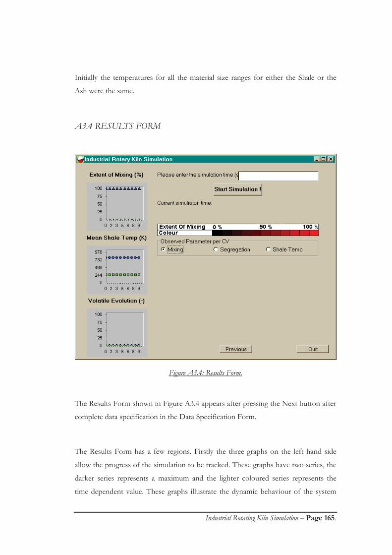
Industrial Rotating Kiln Simulation – Page 165.
Initially the temperatures for all the material size ranges for either the Shale or the
Ash were the same.
A3.4 RESULTS FORM
Figure A3.4: Results Form.
The Results Form shown in Figure A3.4 appears after pressing the Next button after
complete data specification in the Data Specification Form.
The Results Form has a few regions. Firstly the three graphs on the left hand side
allow the progress of the simulation to be tracked. These graphs have two series, the
darker series represents a maximum and the lighter coloured series represents the
time dependent value. These graphs illustrate the dynamic behaviour of the system

Industrial Rotating Kiln Simulation – Page 166.
and included the Extent Of Mixing as a percentage of the maximum mixing in the
kiln, the mean shale temperature in the kiln and the amount of volatile evolution as a
percentage of the shale feed to the kiln. The total duration of the simulation time
could be specified in the Edit box in the top right hand corner. The change in the
control volumes of the grid as specified in Figure 8.2 could be tracked.
Three parameters could be tracked in the different control volumes. These were the
extent of mixing or the mean particle size or the mean temperature in each control
volume. The results of these in the grid were represented by different shades of blue,
green or red respectively.
Images of the Results Form of the simulation are provided in the next section for
different stages of the scenario of Case 2 as presented in Table 9.2.
A3.4.1 Segregation
The initial transverse size distribution for Case 2 is shown in Figure A3.5 and was
represented by different shades of green with the black colour representing a particle
size of 0 mm and a bright green colour representing a particle size of 6.30 mm as
shown in the legend of Figure A3.5.
The shale and the ash particle sizes for Case 2 were different and this is reflected by
the different shaded zones in Figure A3.5. For the initial configuration, the shale was
added to the stagnant layer of the kiln.

Industrial Rotating Kiln Simulation – Page 167.
Figure A3.5: Initial segregation results form (Case 2)
The simulation was run for 60 seconds and at that time the bed was fully segregated.
This is shown in Figure A3.6. As can be seen from the grid system, the mean particle
size in the control volumes closer to the centre of rotation was less than the particle
size of the other control volumes indicated by the darker coloured polygons on the
grid. This showed that the finer material segregated.

Industrial Rotating Kiln Simulation – Page 168.
Figure A3.6: Segregated results form after 60 seconds (Case 2)
It should also be noted that the extent of mixing, the mean shale temp and the
volatile evolution graphs all increased.
A3.4.2 Mixing
Different mixing levels are shown in Figure A3.7. Initially, the grid was coloured
completely black, as the materials were completely unmixed. As time progressed, the
mixing in the control volumes increased and this was shown by the lighter coloured
control volumes in the grid. The mixing was completed after 60 seconds. The darker
region in the centre of the bed was due to the segregated material.

Industrial Rotating Kiln Simulation – Page 169.
A) 5 sec, B) 10 sec, C) 15 sec, D) 20 sec, E) 25 sec, F) 30 sec, G) 40 sec and H) 60 sec
Figure A3.7: Mixing results.

Industrial Rotating Kiln Simulation – Page 170.
Appendix 4: Papers submitted or published.
A4.1 UNREFEREED CONFERENCE PUBLICATIONS D. Van Puyvelde, “Simulation of oil evolution from oil shale in a rotary kiln” in 3rd
Australian Student Particle Technology Conference, Uni. of
Newcastle, Newcastle, New South Wales, Australia (1998).
A4.2 REFEREED CONFERENCE PUBLICATIONS D.R. Van Puyvelde, B.R. Young, M.A. Wilson, “Simulation of the mixing and
segregation in an industrial rotating drum” in Proc. of the 28th Aust. & New
Zealand Chem. Eng. Conf., IEAust, Perth, Western Australia,
Australia (2000).
D. R. Van Puyvelde, B. R. Young, M. A. Wilson, S., J., Schmidt,
“Determination of transverse segregation in a rolling drum using image
processing” in Proc. of the 27th Aust. & New Zealand Chem. Eng.
Conf., IEAust, Newcastle, New South Wales, Australia (1999).
D. Van Puyvelde, B. Young, M. Wilson, J. Schmidt, “Experimental determination
of mixing kinetics in a rolling drum”, Proc. of the 26th Aust. & New
Zealand Chem. Eng. Conf., IEAust, Port Douglas, Queensland,
Australia (1998).
D. Van Puyvelde, B. Young, M. Wilson, J. Schmidt, “Dynamic modelling of
transverse mixing in a rotary kiln” in Proc. of the 25th Aust. & New
Zealand Chem. Eng. Conf., IEAust, Rotorua, New Zealand (1997).
A4.3 INTERNATIONAL REFEREED JOURNAL PUBLICATIONS D.R. Van Puyvelde, B.R. Young, M.A. Wilson, “Simulating the mixing and
segregation behaviour of solids in a rotating kiln”, Comp. Chem. Eng.,
Submitted, (Apr 2000).

Industrial Rotating Kiln Simulation – Page 171.
D.R. Van Puyvelde, B.R. Young, M.A. Wilson, “Comparison of transverse mixing
kinetic data obtained from a rolling drum”, Powder Technol., Submitted,
(2000).
D.R. Van Puyvelde, B. R. Young, M. A. Wilson, S. J. Schmidt, “Modelling
transverse segregation in a rolling drum”, Trans. I. Chem. E. Res. Dev.,
78A, 643-650 (2000).
D.R. Van Puyvelde, B., R., Young, M., A., Wilson, S., J., Schmidt, “Modelling
transverse mixing in a rotating drum”, Can. J. Chem. Eng., 78, 1-8 (2000).
D. R. Van Puyvelde, B., R., Young, M., A., Wilson, S., J., Schmidt,
“Experimental determination of transverse mixing in a rotating drum”, Powder
Tech., 106, 183-191 (1999).