industrial pretreatment advanced local limits

Industrial Pretreatment Advanced Local Limits

NACWA – Providence RIMay 15, 2018 Training[40 CFR §§ 403.5(c) & (d)]

•2018 Update

Pretreatment Program Goals

PREVENT:

– pass through– interference– sludge contamination – POTW worker health/safety risks

“Technically Based Local Limits”

Eleventh Commandment: “Thou Shalt Neither Covet Nor Steal Thy Neighbor’s Local Limits”Keep in mind the definition of “local” [i.e. site specific…YOUR site]Local limits should support and accommodate the strengths and weaknesses of each POTW

Local Limits Address Site Specific Concerns:

Correct existing problemsPrevent potential problemsProtect the receiving watersImprove sludge disposal optionsProtect POTW personnel

Local Limits Site-Specific Factors

POTW Treatment EfficienciesNPDES Permit ComplianceCondition of Receiving WatersWQ Standards for Receiving WatersSludge Disposal Method(s)Worker Health and Safety

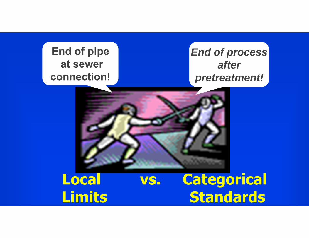
Local vs. CategoricalLimits Standards

End of pipeat sewer

connection!

End of processafter

pretreatment!

Categorical Standards Local Limits

Developed: By EPA (Control Authority) POTW

Objective: Uniform National Control of certain IUs

POTW/Receiving Water Protection

Regulates: Industries specified in Clean Water Act

All non-domestic dischargers

Pollutants: Priority Pollutants (toxic & non-conventional only) Any Pollutant

Basis: Technology Based Technically based on site-specific factors

Apply: At the End of regulated process(es)

Depends on development method

Manufacturing Processes

Technologies, BPT, BAT, BCT

LimitLimit

Limit Limit LimitLimit

TECHNOLOGY BASED LIMIT DEVELOPMENT

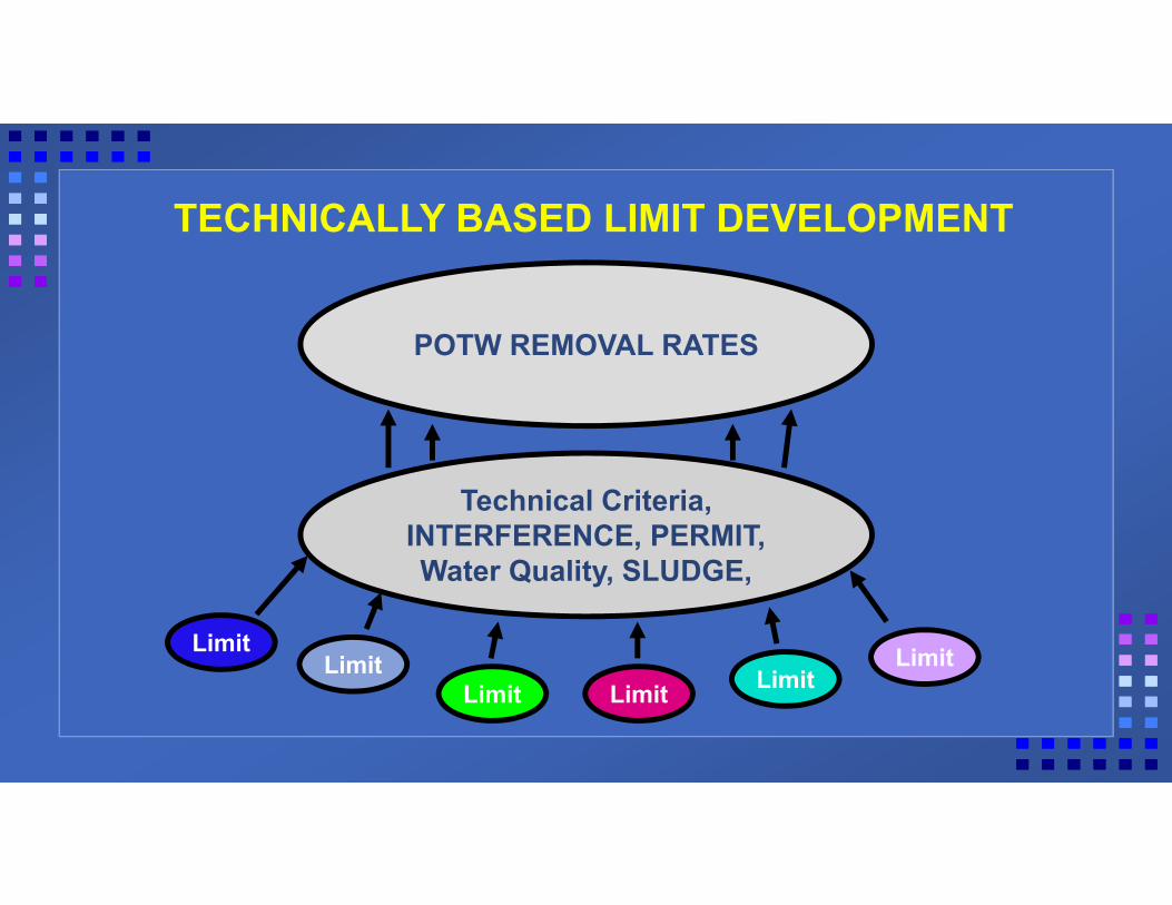
POTW REMOVAL RATES

Technical Criteria, INTERFERENCE, PERMIT, Water Quality, SLUDGE,

LimitLimit

Limit Limit LimitLimit

TECHNICALLY BASED LIMIT DEVELOPMENT

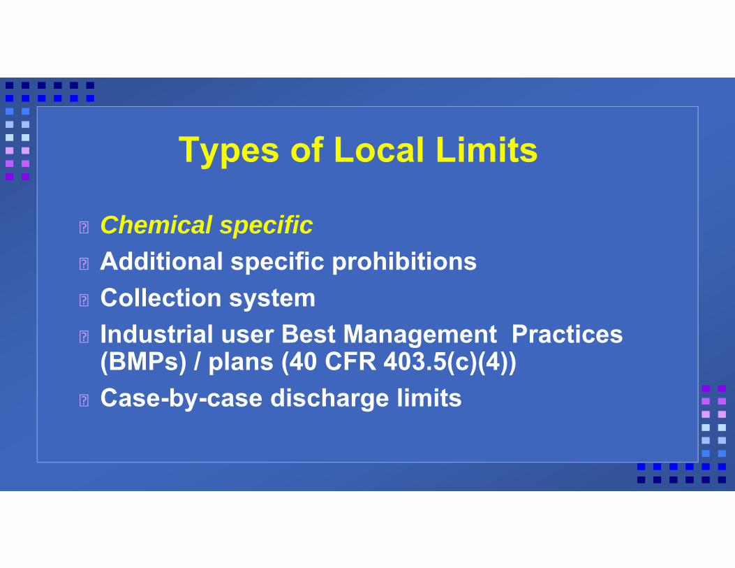
Types of Local Limits

Chemical specificAdditional specific prohibitionsCollection systemIndustrial user Best Management Practices (BMPs) / plans (40 CFR 403.5(c)(4))Case-by-case discharge limits

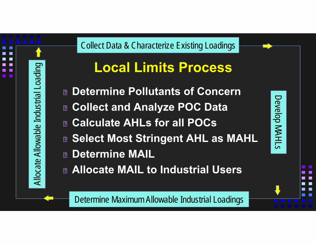
Local Limits ProcessDetermine Pollutants of Concern Collect and Analyze POC DataCalculate AHLs for all POCsSelect Most Stringent AHL as MAHLDetermine MAILAllocate MAIL to Industrial Users

Collect Data & Characterize Existing LoadingsDevelop MAHLs

Determine Maximum Allowable Industrial Loadings

Alloc

ate A

llowa

ble In

dustr

ial Lo

ading

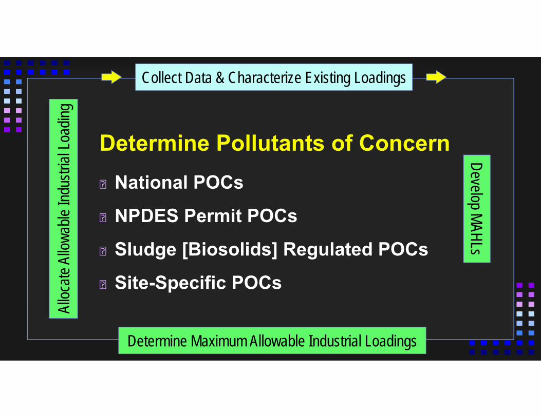
Determine Pollutants of ConcernNational POCs

NPDES Permit POCs

Sludge [Biosolids] Regulated POCs

Site-Specific POCs



Alloc

ate A

llowa

ble In

dustr

ial Lo

ading

Pollutants of Concern [POC]Any pollutant which might be reasonably discharged and capable of causing:– pass through– interference– sludge contamination – POTW worker health/safety risks

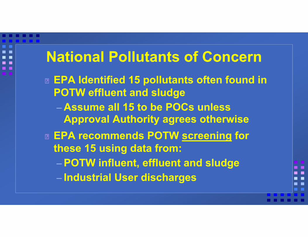
National Pollutants of ConcernEPA Identified 15 pollutants often found in POTW effluent and sludge– Assume all 15 to be POCs unless

Approval Authority agrees otherwiseEPA recommends POTW screening for these 15 using data from:– POTW influent, effluent and sludge– Industrial User discharges

National EPA POCs

Arsenic Lead SilverCadmium Mercury ZincChromium Molybdenum BOD5

Copper Nickel TSSCyanide Selenium Ammonia

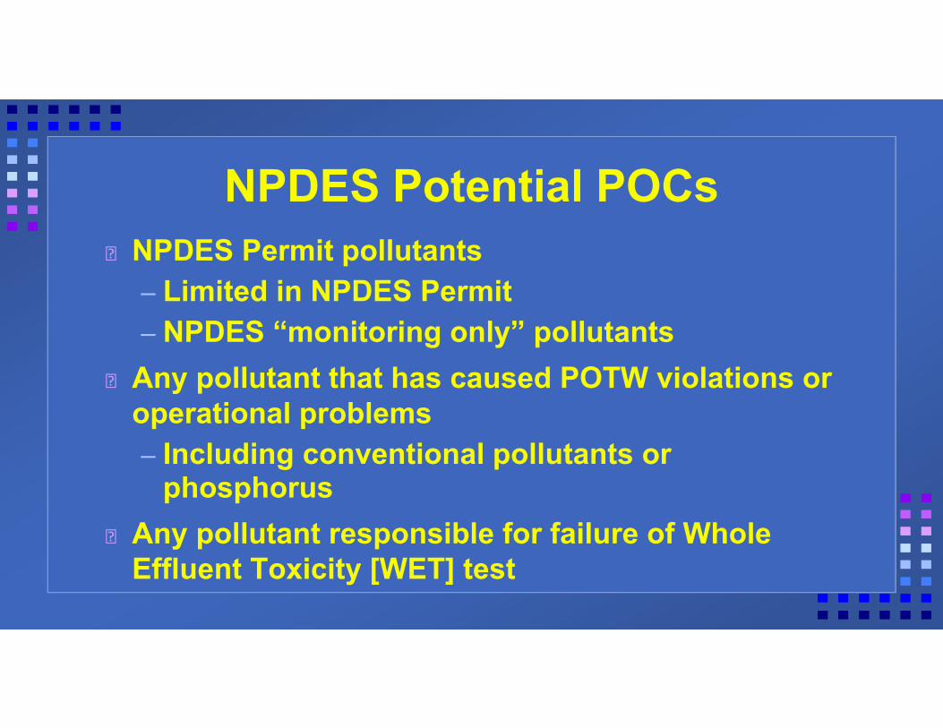
NPDES Potential POCsNPDES Permit pollutants– Limited in NPDES Permit – NPDES “monitoring only” pollutants

Any pollutant that has caused POTW violations or operational problems– Including conventional pollutants or

phosphorusAny pollutant responsible for failure of Whole Effluent Toxicity [WET] test

Biosolids Regulated POCsLand Application: [40 CFR Part 503]– Arsenic, cadmium, copper, lead, mercury,

molybdenum, nickel, selenium, zincSurface Disposal: [40 CFR Part 503]– Arsenic, chromium, nickel

Incineration: [40 CFR Parts 503 and 60]– Beryllium, mercury, lead, arsenic, cadmium,

chromium, nickel, dioxins, furansAny State regulated pollutants

Site Specific Potential POCsPOTW Interference [no NPDES violations]Pollutants detected in Priority Pollutant ScanReclaim Water [Effluent] Reuse LimitsAir Quality Standards [NESHAP, NAAQS]POTW Receiving Water Issues:– Public/Private Drinking Water Supply– Outstanding Resource Waters

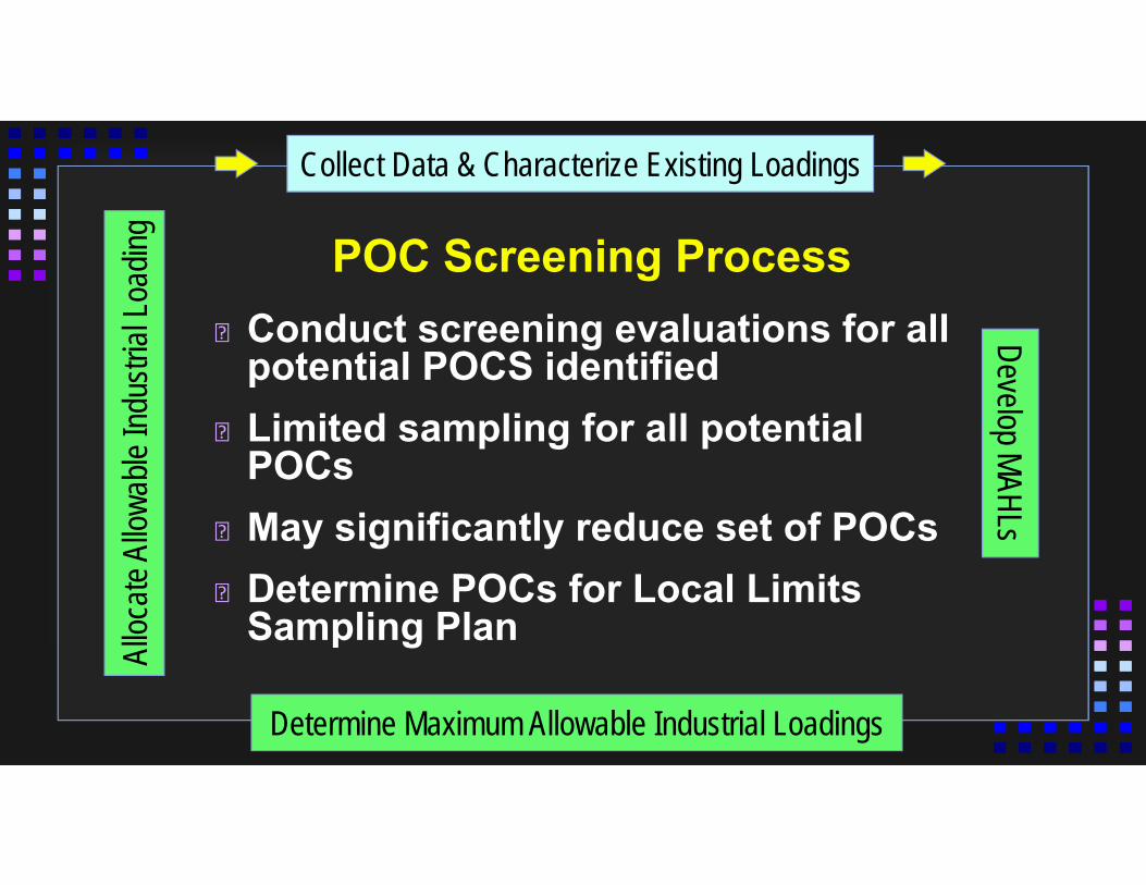
POC Screening ProcessConduct screening evaluations for all potential POCS identifiedLimited sampling for all potential POCs May significantly reduce set of POCsDetermine POCs for Local Limits Sampling Plan



Alloc

ate A

llowa

ble In

dustr

ial Lo

ading

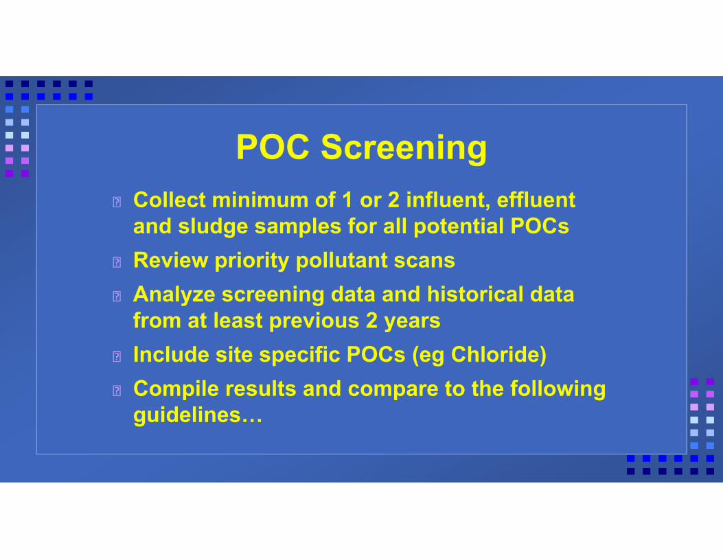
POC ScreeningCollect minimum of 1 or 2 influent, effluent and sludge samples for all potential POCsReview priority pollutant scansAnalyze screening data and historical data from at least previous 2 yearsInclude site specific POCs (eg Chloride)Compile results and compare to the following guidelines…

You Know You’re a POC if the…Maximum POTW effluent concentration is >50% of effluent limit based on water quality criteriaMaximum sludge concentration is >50% of applicable sludge criteriaMaximum POTW influent grab sample concentration is >50% of inhibition threshold

You Know You’re a POC if the…Maximum POTW influent 24-hr composite is >25% of inhibition thresholdMaximum POTW influent concentration is >0.2% of applicable sludge criteriaPOTW influent concentration [adjusted for receiving stream dilution] exceeds water quality criteria/standards

Local Limits Development Data

Background InformationDevelop Sampling PlanCollect and Analyze Samples Data Review and Evaluation



Alloc

ate A

llowa

ble In

dustr

ial Lo

ading

Local Limits Data Used to:Identify/confirm presence of pollutantsDetermine POCsDetermine current POTW loadingsCalculate % Removal EfficienciesDetermine site-specific inhibition valuesEstimate loadings from IUs, domestic/ uncontrollable sources, etc.

Removal Rate Formula:

Removal Rate [Efficiency] (as decimal) =

Influent (mg/l) – Effluent (mg/l) Influent (mg/l)

Note….mass in pounds/day can also be used for this calculation

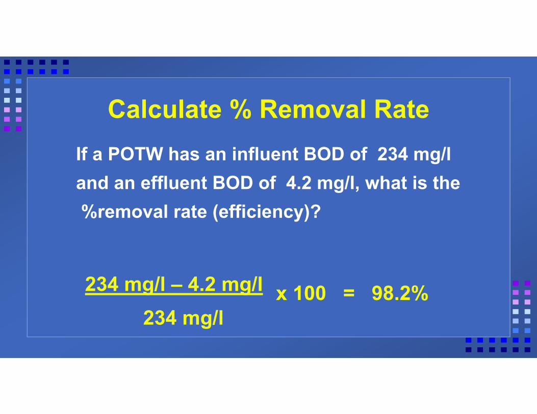
Calculate % Removal RateIf a POTW has an influent BOD of 234 mg/l and an effluent BOD of 4.2 mg/l, what is the%removal rate (efficiency)?

234 mg/l – 4.2 mg/l x 100 = 98.2%234 mg/l

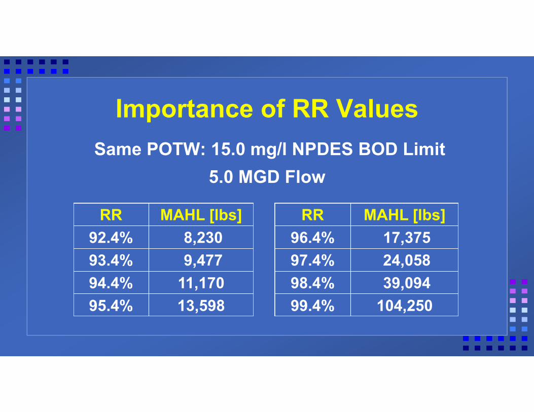
Importance of RR ValuesSame POTW: 15.0 mg/l NPDES BOD Limit

5.0 MGD Flow

RR MAHL [lbs]92.4% 8,23093.4% 9,47794.4% 11,17095.4% 13,598

RR MAHL [lbs]96.4% 17,37597.4% 24,05898.4% 39,09499.4% 104,250

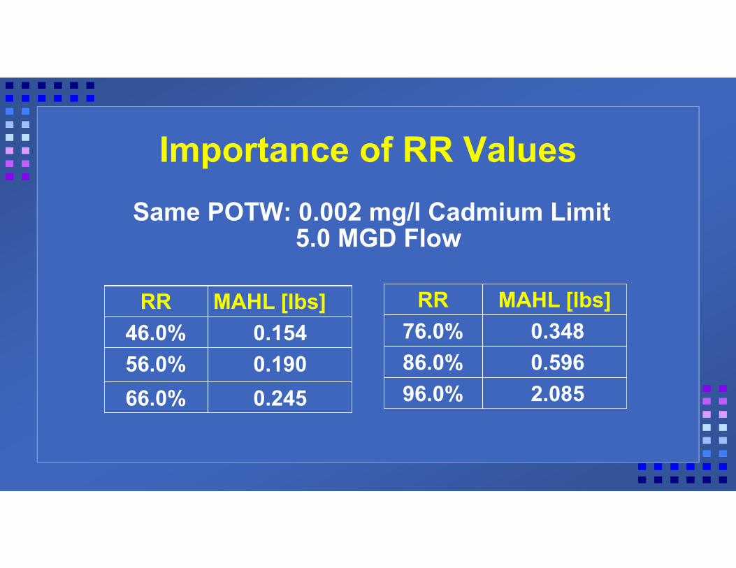
Importance of RR ValuesSame POTW: 0.002 mg/l Cadmium Limit

5.0 MGD Flow

RR MAHL [lbs]46.0% 0.15456.0% 0.19066.0% 0.245

RR MAHL [lbs]76.0% 0.34886.0% 0.59696.0% 2.085

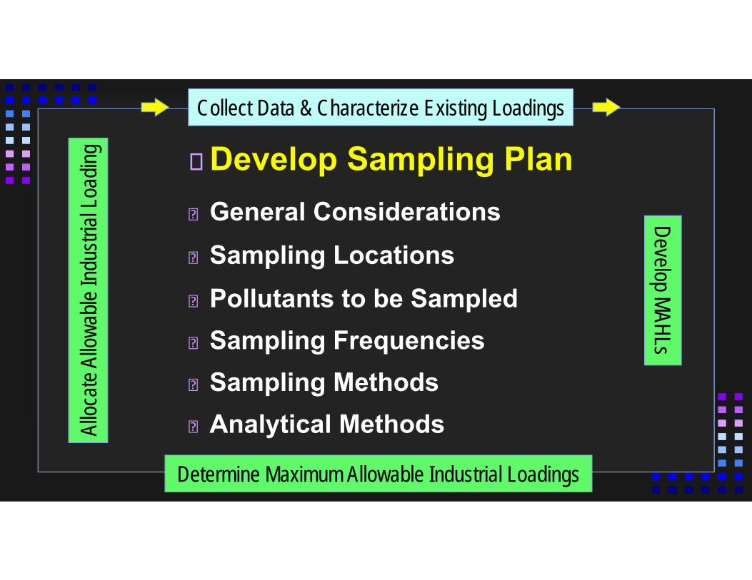
Develop Sampling PlanGeneral ConsiderationsSampling LocationsPollutants to be SampledSampling FrequenciesSampling MethodsAnalytical Methods



Alloc

ate A

llowa

ble In

dustr

ial Lo

ading

General Considerations:NPDES Monitoring: “Daily” [Mon-Fri]– Use all NPDES Data for POC– “Composite Times” of NPDES samples – If only effluent analysis is NPDES required,

look at resources for doing influent, tooDon’t sample on same day of week for every POC sampling event [You’ll see why later…]Quarterly Sampling * 5 yrs = 20 data points

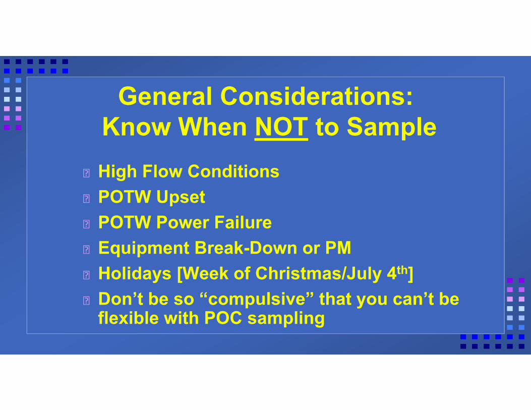
General Considerations:Know When NOT to SampleHigh Flow ConditionsPOTW UpsetPOTW Power FailureEquipment Break-Down or PMHolidays [Week of Christmas/July 4th]Don’t be so “compulsive” that you can’t be flexible with POC sampling

POTW Sampling LocationsPOTW Influent* – Before mixing with any recycle streams

POTW Effluent* Aerobic/Anaerobic Digester*– “Acclimation” values

Biosolids to Disposal*– 40 CFR Part 503 Annual Report Data

Activated Sludge– “Acclimation” values

Other Sampling Locations:

Domestic/Uncontrollable Site(s)– May Need Several Locations Due to:

»Variability, different H20 sources SIUs – May Have Historical Data on some/all POCs

Hauled Waste– Depends on Type(s) Accepted at POTW

Pollutants to Be Sampled:“The EPA 15”-National POCsPOTW Site Specific POCsOrganic “Priority Pollutants”– POTW Influent/Effluent Only% Solids in SludgeTCLP pollutants – Sludge for Landfill Disposal

Sampling Days for Initial Local Limits Development

ParameterPOTW Domestic/

UncontrollableInfluent Effluent SludgeOrganic PP 1 - 2 1 - 2 1 1 - 2National POC 7 - 14 7 - 14 2 7Site Sp. POC 7 - 14 7 - 14 2 7

% Solids 2

TCLP [Landfill] 1

Sampling FrequenciesSampling should be random and representative of different days, months and IU production schedulesPOC Sampling schedule should ensure collection of samples that are representative of weather conditions that affect POTWsPOTW Sampling should account for hydraulic detention [retention] times

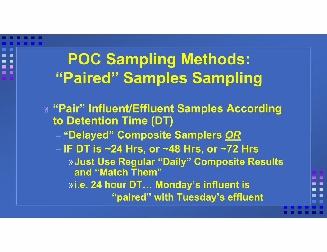
POC Sampling Methods:“Paired” Samples Sampling

“Pair” Influent/Effluent Samples According to Detention Time (DT)– “Delayed” Composite Samplers OR– IF DT is ~24 Hrs, or ~48 Hrs, or ~72 Hrs

»Just Use Regular “Daily” Composite Results and “Match Them”

»i.e. 24 hour DT… Monday’s influent is “paired” with Tuesday’s effluent

POC SAMPLING:“Paired” Samples Sampling

DETENTION TIME (DT) FORMULA:

POTW Detention Time [in hours] =24 [hr/day] * POTW Tank Volumes [MG]

Actual POTW Flow [MGD]

Math Exercise: Calculate Detention Time

Tank Volumes [look in POTW O&M Manual]

– Primary Clarifiers = 0.40 MG– Aeration Tanks = 1.40 MG– Final Clarifiers = 0.60 MG– Chlorine Contact Tank = 0.105 MGPermitted Flow = 4,000,000 gpdActual Flow = 2,250,000 gpd

Calculate Detention Time [DT]TV = 0.4 + 1.4 + 0.6 + 0.105 = 2.505 MG

Actual Flow = 2,250,000 gpd = 2.250 MGD1,000,000 gal/MG

DT = 24 (hr/day) * Tank Volume [MG]Actual Flow [MGD]

DT = 24 (hr/day) * 2.505 MG2.250 MGD

= 26.72 hours

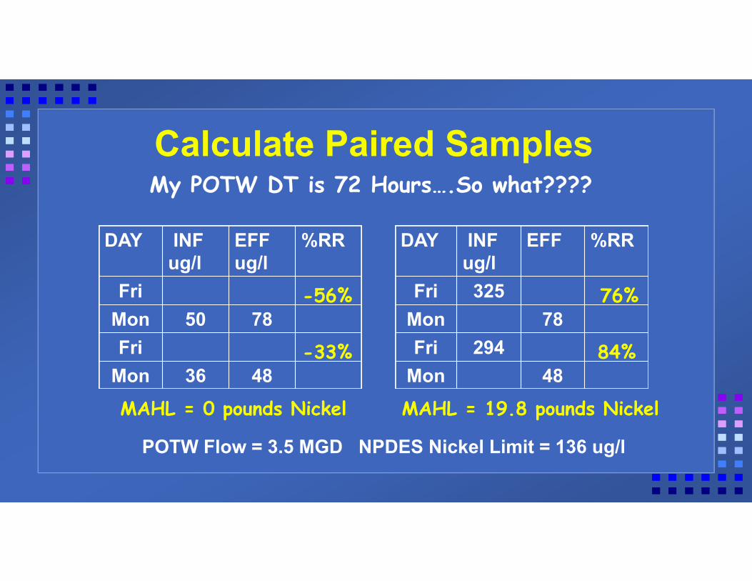
Calculate Paired Samples

DAY INF ug/l

EFF ug/l

%RR

FriMon 50 78Fri

Mon 36 48

POTW Flow = 3.5 MGD NPDES Nickel Limit = 136 ug/l

MAHL = 19.8 pounds NickelMAHL = 0 pounds Nickel

DAY INF ug/l

EFF %RR

Fri 325Mon 78Fri 294

Mon 48

My POTW DT is 72 Hours….So what????

-56%

-33%

76%

84%

Sampling MethodsGrab Samples [at least 4]– Single “dip and take”“Grab Composites”

»Grabs combined into one sample»Analyzed separately and averaged

24-Hour Composite Samples– Time Composite– Flow Proportioned

Typical Wastewater Sample TypesGrab Sample Composite Sample

pH BOD/CBODCyanide COD

Total Phenol TSS/TDSOil and Grease Nutrients [Nitrogen/Phosphorus]

Sulfides Metals [except 1669 level]Flashpoint Whole Effluent Toxicity

Volatile Organic Compounds [Method 624]

Acid Extractable/Base Neutral Organics [Method 625]

POC Sampling Methods:Whole Effluent Toxicity

Several 24-Hour Composites Used For WET– Coordinate POC Analyses with WET…..

»POTW Influent and EffluentMetals Cyanide NutrientsOrganics

»Aeration Tank Samples for Inhibition, Too!!!

40 CFR Part 136EPA regulation governing all NPDES and PT program wastewater analyses– Approved analytical methods– Required preservation, containers,

holding timesRecent Amendments removed some of the older Std. Methods editions

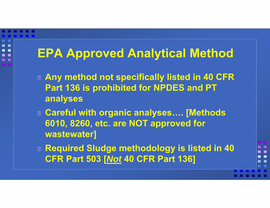
EPA Approved Analytical Method

Any method not specifically listed in 40 CFR Part 136 is prohibited for NPDES and PT analysesCareful with organic analyses…. [Methods 6010, 8260, etc. are NOT approved for wastewater] Required Sludge methodology is listed in 40 CFR Part 503 [Not 40 CFR Part 136]

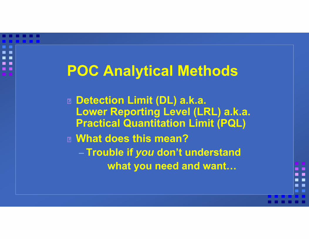
POC Analytical Methods

Detection Limit (DL) a.k.a. Lower Reporting Level (LRL) a.k.a. Practical Quantitation Limit (PQL)What does this mean?– Trouble if you don’t understand

what you need and want…

POC Analytical Methods:Metals, Metals Everywhere“REGULAR LEVEL” METALS ANALYSES– Flame Atomic Absorption [AA]– ICP [“Plasma”]

“LOW LEVEL” METALS ANALYSES– Graphite Furnace Atomic Absorption– ICP/MS [Plasma Mass Spec]

“Regular Level” Metals Removal Rate Example

Chromium Influent = 11 ug/lChromium Effluent = <10 ug/l– Some States will let you use ½ DL on the

effluent value [10 * ½ = 5 ug/l] 11 – 5 * 100

11 = 54.5 % RR

[OR EPA Median Literature Value of 82%] VERSUS………….

“Low Level” Metals Removal Rate Example

Same POC Samples analyzed by ICP-MSChromium Influent = 11 ug/lChromium Effluent = 0.70 ug/l

11 – 0.70 * 100 = 93.6% RR11

[Oh what a difference ICP/MS makes!]

SAME POTW…SAME SAMPLES….

Source/Type of Metals Analysis

Removal Rate %

Allowable Influent

Chromium

Chromium MAHL

(pounds)“Regular Level” 54.5% 0.11 mg/l 4.6Median Literature 82% 0.28 mg/l 11.7“Low Level” 93.6% 0.78 mg/l 32.5

5.0 MGD Flow and 0.050 mg/l Effluent Limit

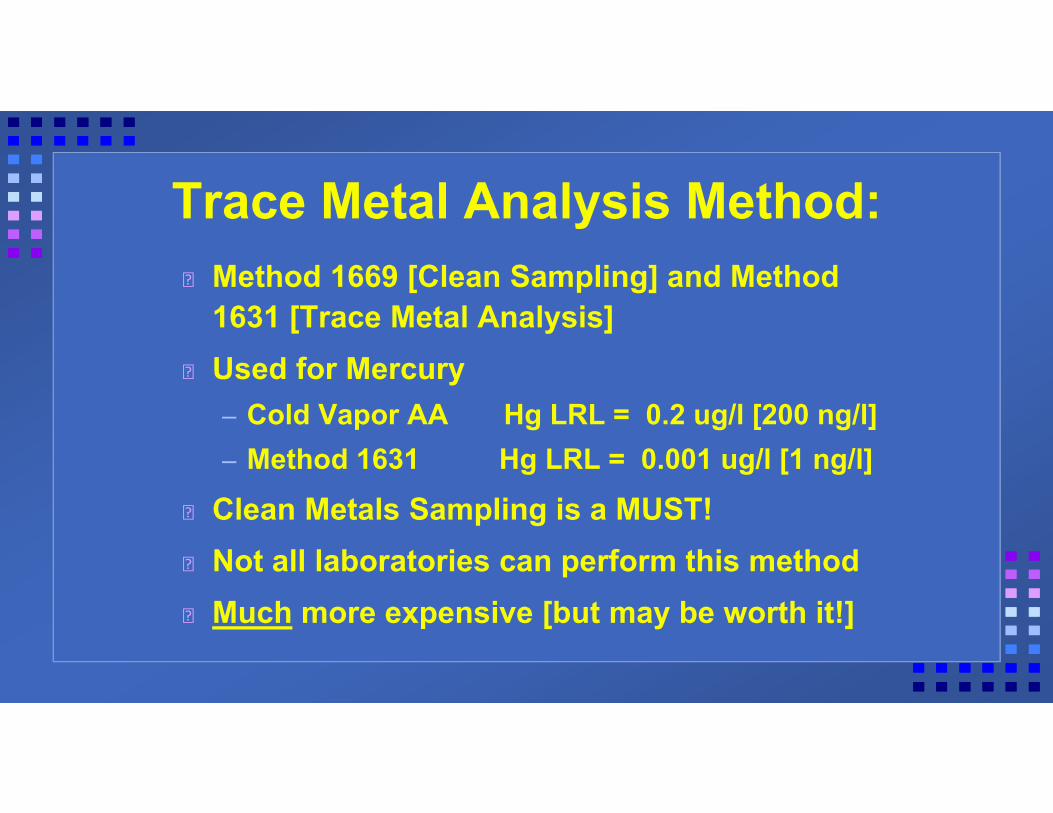
Trace Metal Analysis Method:Method 1669 [Clean Sampling] and Method 1631 [Trace Metal Analysis]Used for Mercury– Cold Vapor AA Hg LRL = 0.2 ug/l [200 ng/l]– Method 1631 Hg LRL = 0.001 ug/l [1 ng/l]

Clean Metals Sampling is a MUST!Not all laboratories can perform this methodMuch more expensive [but may be worth it!]

Something Else to Consider..

POTW Flow = 3.5 MGD NPDES NH3-N Limit = 2.0 mg/l

INF EFF RR %12.5 <0.5 96.014.0 <0.5 96.410.8 <0.5 95.415.5 <0.5 96.8

ADRE 96.15

INF EFF RR %12.5 <0.1 99.214.0 <0.1 99.310.8 <0.1 99.115.5 <0.1 99.4

ADRE 99.25

MAHL = 7784 pounds NH3NMAHL = 1516 pounds NH3N

POC Data Review

Review POC Sampling Plan Data – Is the POC Data Valid? Does it Make Sense?– Is the Pollutant Present in the Influent?

» If not, can it be an internal POTW process?– Is the POTW….Compliant? Noncompliant?

Look at historical removal efficiencies– How do they compare with what YOU got?

Audit Laboratory [POTW and Commercial]

REVIEW DATA SET

Review Data and Look for…..– Unusually low Daily Removal Efficiency– Pattern of increasing effluent values with no

similar influent increase– Corresponding inf/eff extreme values– CHECK YOUR MATH [and computer’s math]

»unit conversions [0.0873 mg/l = 87.3 ug/l]– Will “hydraulic sampling” make it better???

DATA EXCLUSIONTechnical or Operational Problems at POTW– Fix it…then take extra POC samples

Negative Daily Removal Efficiency– Maybe…why? Paired Resample?

QA/QC Problems in the Lab– All influent and effluent samples BDL

»Elevated Detection Limits?– Metals, Metals Everywhere?– “Impossible Values”– Reanalyze [if possible] or Resample

Data Review

Date: Influent Effluent1-9-01 < 2.0 mg/l <2.0 mg/l

1-10-01 175 mg/l <2.0 mg/l1-11-01 256 mg/l <2.0 mg/l1-16-01 209 mg/l <2.0 mg/l

Actual POC BOD Values*:

*From Commercial Laboratory, not POTW Laboratory

PICK THE NUMBER!!!!

98.43% or 98%?98.78% or 98.8%?95.5% or 96%?

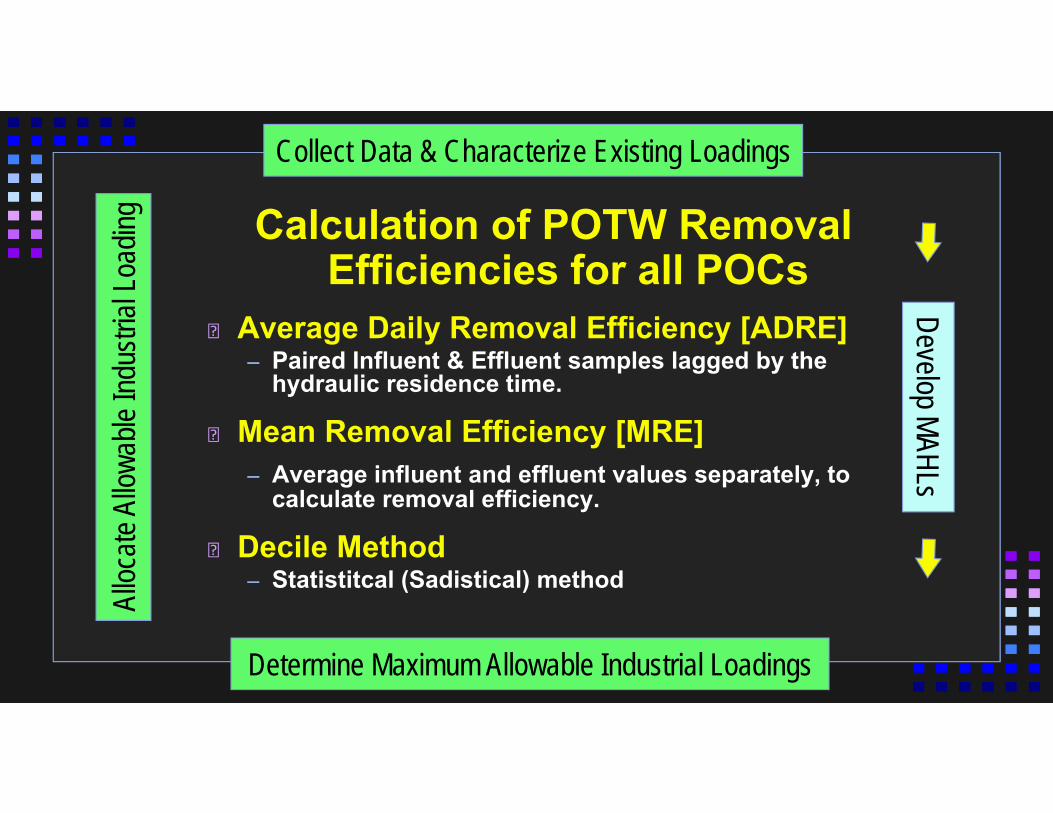
Calculation of POTW Removal Efficiencies for all POCs

Average Daily Removal Efficiency [ADRE]– Paired Influent & Effluent samples lagged by the

hydraulic residence time.

Mean Removal Efficiency [MRE]– Average influent and effluent values separately, to

calculate removal efficiency.

Decile Method– Statistitcal (Sadistical) method



Alloc

ate A

llowa

ble In

dustr

ial Lo

ading

Average Daily Removal Efficiency (ADRE)

Rpotw = Plant removal efficiency from headworks to plant effluent (as decimal)In= WWTP influent pollutant concentration atheadworks , mg/LEpotw, n = WWTP effluent pollutant concentrationn = paired observations, numbered 1 to N

Sample Day Influent Load (lbs)

Effluent Load (lbs)

DRE %

1 518.22 111.41 78.502 163.98 173.99 -6.103 110.15 97.64 11.364 1739.93 474.41 72.735 2301.00 97.88 95.756 170.48 105.15 38.327 473.16 132.67 71.968 314.19 148.96 52.599 306.68 132.69 56.73

ADRE 52.43

ADRE - Hypothetical Zinc loadings

Rpotw

=

___________518.22 – 111.41

518.22+ etc = 4.7184

9x 100 = 52.43%

Average Daily Removal Efficiency (ADRE)

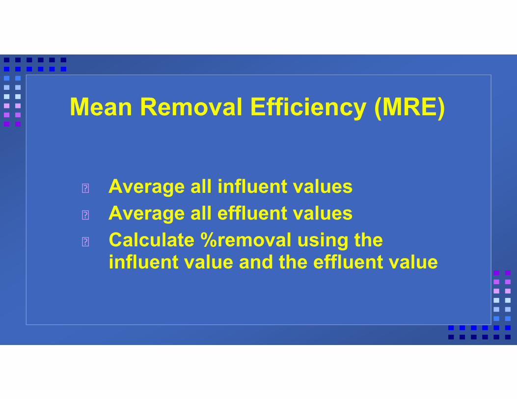
Mean Removal Efficiency (MRE)

Average all influent values Average all effluent values Calculate %removal using the influent value and the effluent value

Rpotw = Plant removal efficiency from headworks toplant effluent (as decimal)Ir = WWTP influent pollutant concentration atheadworks, mg/lEpotw, t = WWTP effluent pollutant concentration, mg/lt = plant effluent samples, numbered 1 to Tr = plant influent samples, numbered 1 to R


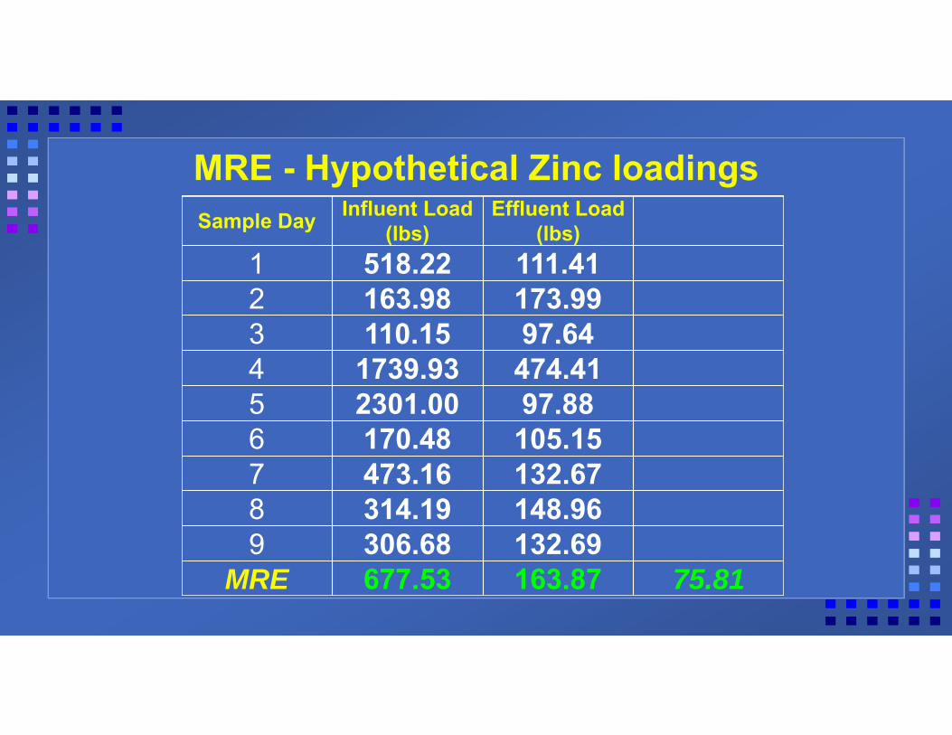
Sample Day Influent Load (lbs)

Effluent Load (lbs)

1 518.22 111.412 163.98 173.993 110.15 97.644 1739.93 474.415 2301.00 97.886 170.48 105.157 473.16 132.678 314.19 148.969 306.68 132.69

MRE 677.53 163.87 75.81

MRE - Hypothetical Zinc loadings

Rpotw = ___________677.53 – 163.87

677.53= 0.75814 x 100 = 75.81%


Decile Method

Requires at least nine daily removal efficiency values based on paired sets of influent and effluent data.Sort daily removal efficiency data from lowest to highest and calculate the percentage of removal efficiencies above or below the specified removal efficiency.

Sample Day

Influent Load (lbs)

Effluent Load (lbs)

DRE%

Deciles

2 163.98 173.99 -6.10 1st=10%3 110.15 97.64 11.36 2nd=20%6 170.48 105.15 38.32 3rd=30%8 314.19 148.96 52.59 4th=40%9 306.68 132.69 56.73 5th=50%7 473.16 132.67 71.96 6th=60%4 1739.93 474.41 72.73 7th=70%1 518.22 111.41 78.50 8th=80%5 2301.00 97.88 95.75 9th=90%

DECILE - Hypothetical Zinc Loadings

Decile Method

Similar to a data set median but divides the data set into 10 equal parts.10% of the data is below the 1st decile, 20% is below the 2nd decile and so on.The 5th decile = data set median.This hypothetical POTW has an overall plant removal efficiency Rpotw of 56.73%less than half the time

Method Removal Rate ComparisonsSame Data Set

ADRE 52.43%

MRE 75.81%

5th DECILE 56.73%

Removal Efficiencies Derived from Sludge Data

For conservative pollutants such as metals, POTWs can use sludge data to estimate removal efficiency, Rpotw.

Sludge data should be used in place of effluent data when a POTW has influent data above detection, but does not have adequate effluent data above detection.

Removal Efficiencies Derived from Sludge Data

Data Required for Sludge Removal Efficiencies– Sludge flow to disposal in MGD– Percent solids of sludge to disposal– Sludge pollutant concentration in mg/kg– Specific gravity of sludge in kg/L– WWTP average flow in MGD

Paired data used for ADRE approachMean of individual data used for MRE approach

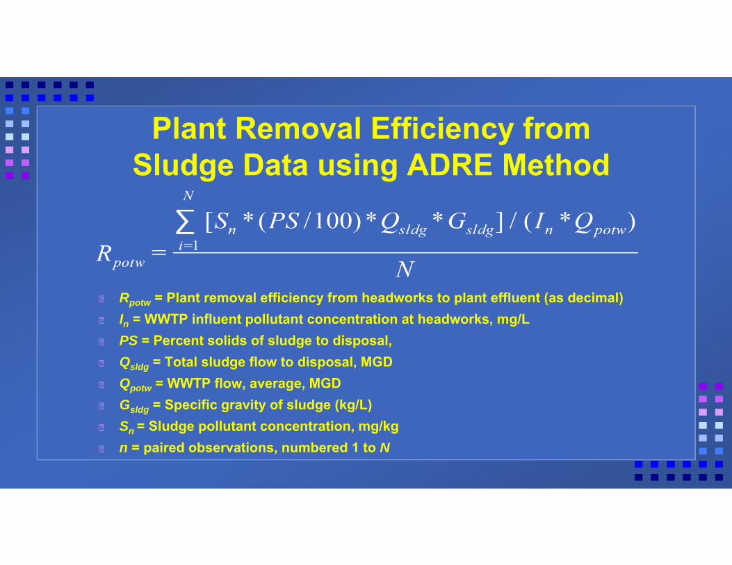
Rpotw = Plant removal efficiency from headworks to plant effluent (as decimal)In = WWTP influent pollutant concentration at headworks, mg/LPS = Percent solids of sludge to disposal,Qsldg = Total sludge flow to disposal, MGDQpotw = WWTP flow, average, MGDGsldg = Specific gravity of sludge (kg/L)Sn = Sludge pollutant concentration, mg/kgn = paired observations, numbered 1 to N

Plant Removal Efficiency from Sludge Data using ADRE Method

Plant Removal Efficiency From Sludge Data Using MRE Method

Rpotw = Plant removal efficiency from headworks to plant effluent (as decimal)Ir= WWTP influent pollutant concentration at headworks, mg/LPS = Percent solids of sludge to disposal,Qsldg = Total sludge flow to disposal, MGDQpotw = WWTP flow, average, MGDGsldg = Specific gravity of sludge (kg/L)8.34 = unit conversion factorSu = Sludge pollutant concentration, mg/kgu = sludge samples, numbered 1 to Ur = influent samples numbered 1 to R

Guidance On Using Different Methodologies

MRE recommended over the ADRE by EPA if less than 10 pairs are available.

Decile approach allows for comprehensive view, and considers daily removal efficiency variation.

Individual decile estimates, depending on how conservative the POTW wants to be, can be less precise than the ADRE and MRE estimates.

Options for Managing Sampling Results Below the Method Detection Level (“BDL”)

in Removal Efficiency CalculationsIf only a few data values are BDL: If most data values are BDL:

Option 1: Use surrogate value of ½ ML.

Option 1: Re-evaluate the need for a local limit for the pollutant. (However, if the pollutant is one of the 15 EPA POCs an AHL should be developed.)

Option 2: Discard the few samples below the ML. (Influent and effluent data should be discarded in pairs.)

Option 2: Use removal rate data from other plants. (LL Manual Section 5.1.4.)

OTHER OPTIONS:

Use other statistical methods: Regression order statistics, probability plotting and maximum likelihood estimations are discussed in

Appendix Q of EPA LL Manual

Negative Removal EfficienciesCauses:– POTW’s do not operate at steady state– Analytical problems (e.g., false positives with

CN-)– Data not paired with POTW detention time– Contaminated treatment chemicals

Negative removal efficiencies should always be investigated – Should not be dismissed unless there is adequate technical justification Handle non-detect samples as previously discussed

Using EPA’s Default Removal Efficiencies

EPA recommends site specific dataIf site specific data are inadequate, removal efficiencies for some pollutants from other POTWs or studies are given in EPA Local Limits Guidance Manual– Caution

»Some EPA data is from 1977 studies»EPA uses the most restrictive (lowest) values

Develop Maximum Allowable Headworks [MAHL] LoadingSelect most stringent AHL as MAHL:– Effluent Quality (NPDES Permit Limits)– Water Quality Standards [Pass-thru] – Resource Protection– Interference (Inhibition)– Sludge Contamination (40CFR 503)– Air Quality Standards– Other (eg worker safety)



Alloc

ate A

llowa

ble In

dustr

ial Lo

ading

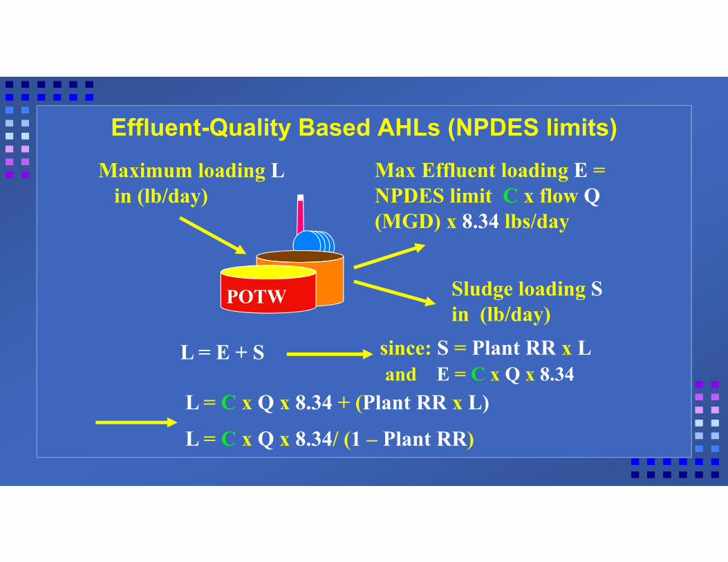
Max Effluent loading E = NPDES limit C x flow Q(MGD) x 8.34 lbs/day

Effluent-Quality Based AHLs (NPDES limits)

POTW

Maximum loading Lin (lb/day)

Sludge loading Sin (lb/day)

L = E + S since: S = Plant RR x L

L = C x Q x 8.34 + (Plant RR x L)and E = C x Q x 8.34

L = C x Q x 8.34/ (1 – Plant RR)

AHLnpdes = Allowable headworks loading based on NPDES permit requirements, lbs/dayCnpdes = NPDES permit limit, mg/LQpotw = WWTP flow, average, MGDRpotw = Plant removal efficiency from headworks to plant effluent (as decimal)8.34 = conversion factor

Effluent-Quality Based AHLs

AHLwq = Allowable headworks loading based on water quality, lbs/dayCstr = Receiving stream background concentration, mg/LCwq = State WQS or EPA WQC, mg/LQstr = Receiving stream (upstream) flow, MGDQpotw = WWTP flow, average, MGDRpotw = Plant removal efficiency from headworks to plant effluent (as decimal)8.34 = conversion factor

AHL Based on Water Quality CriteriaAHLwq = 8.34[Cwq(Qstr + Qpotw)-(Cstr*Qstr)]

(1 - Rpotw)

Resource Protection AHLsPOTWs that discharge to groundwater resources such as:– Water recharge projects– Saline intrusion barriers– Underground injection projects

May be subject to individual State WQ laws

Inhibition Based AHLs

Secondary and Tertiary Treatment Unit Inhibition– No inhibition problems in the past– Past inhibition problems

»May have difficulty in determining plant inhibition values

»Site specific data are preferred

AHLs Based On Secondary and Tertiary Treatment Inhibition

Lsec = AHL based on secondary treatmentinhibition, lbs/dayLter = AHL based on tertiary treatment inhibition, lbs/dayCinhib2 = Inhibition criteria for secondary treatment, mg/LCinhib3 = Inhibition criteria for tertiary treatment, mg/LQpotw = WWTP flow, MGDRsec = Removal efficiency from headworks to secondary treatment influent (as decimal)Rter = Removal efficiency from headworks to tertiary treatment influent (as decimal)8.34 = unit conversion factor

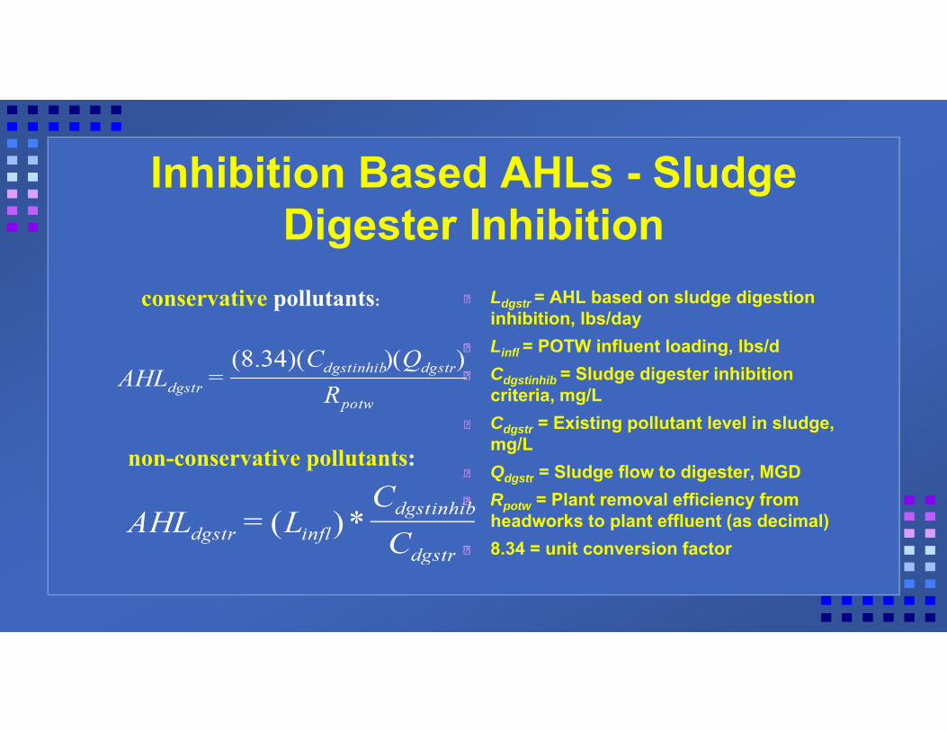
Inhibition Based AHLs - Sludge Digester Inhibition

Ldgstr = AHL based on sludge digestion inhibition, lbs/dayLinfl = POTW influent loading, lbs/dCdgstinhib = Sludge digester inhibition criteria, mg/LCdgstr = Existing pollutant level in sludge, mg/LQdgstr = Sludge flow to digester, MGDRpotw = Plant removal efficiency from headworks to plant effluent (as decimal)8.34 = unit conversion factor

conservative pollutants:

non-conservative pollutants:

Sludge-Quality Based AHLs

Land ApplicationSurface DisposalIncineration

Hazardous Waste

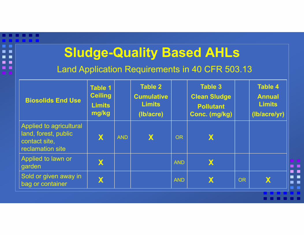
Sludge-Quality Based AHLs

Biosolids End Use

Table 1 CeilingLimits mg/kg

Table 2Cumulative

Limits(lb/acre)

Table 3Clean Sludge

Pollutant Conc. (mg/kg)

Table 4Annual Limits

(lb/acre/yr)

Applied to agricultural land, forest, public contact site, reclamation site

X AND X OR X

Applied to lawn or garden X AND XSold or given away in bag or container X AND X OR X

•Land Application Requirements in 40 CFR 503.13

AHL’s Based on Sludge Land Application Criteria

Determine which land application criteria apply

Determine applicable Table 1, 2, 3 or 4 criteria

Convert Table 2 cumulative loading rates (lb/acre) and Table 4 annual pollutant loading rates (lb/acre/year), to equivalent sludge standards (mg/kg)

Determine lowest sludge standard from all calcs.

Use lowest standard to determine the sludge land –application based AHL for conservative pollutants

Cslgstd = Equivalent sludge standard, mg/kg dry sludgeCcum = Federal or State land application cumulative pollutant loading rate (lbs/acre over the site life)Gsldg = Specific gravity of sludge (kg/L)PS = Percent solids of sludge to disposalQbla = Sludge flow to bulk land application (agricultural, forest, public contact, or reclamation site), MGDSA = Site area, acres SL = Site life, years3046 = unit conversion factor

Converting Cumulative Loading Rates from Table 2 to Dry Sludge Concentrations

Cslgstd = Equivalent sludge standard, mg/kg dry sludgeCann = Federal or State land application annual pollutant loading rate (in lbs/acre/yr)Gsldg = Specific gravity of sludge (kg/L)PS = Percent solids of sludge to disposalQla = Sludge flow to non-bulk land application, MGDSL = Site life, years3046 = unit conversion factor

Converting Annual Loading Rates from Table 4 to Dry Sludge Concentrations

AHLsldg = Allowable headworks loading, lbs/dayCstgstd = Sludge standard, mg/kg dry sludgePS = Percent solids of sludge to disposal,Qsldg = Total sludge flow to disposal, MGDRpotw = Plant removal efficiency from headworks toplant effluent (as decimal)Gsldg = Specific gravity of sludge (kg/L)8.34 = unit conversion factor

AHLs Based on Sludge Land Application and Surface Disposal Criteria (for conservative pollutants)

Guidance On Sludge Quality Based AHLs

EPA recommends using clean sludge levels (40 CFR Part 503 Table 3) Generally, can assume specific gravity is equal to water (1 kg/L)Drier sludges may have a specific gravity greater than 1, but assuming a value of 1 leads to conservative AHLsCan use measured specific gravity

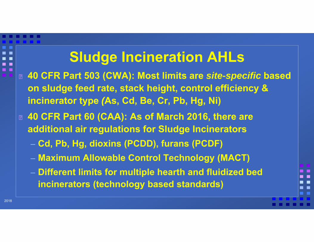
Sludge Incineration AHLs40 CFR Part 503 (CWA): Most limits are site-specific based on sludge feed rate, stack height, control efficiency & incinerator type (As, Cd, Be, Cr, Pb, Hg, Ni) 40 CFR Part 60 (CAA): As of March 2016, there are additional air regulations for Sludge Incinerators – Cd, Pb, Hg, dioxins (PCDD), furans (PCDF)– Maximum Allowable Control Technology (MACT)– Different limits for multiple hearth and fluidized bed

incinerators (technology based standards)•2018

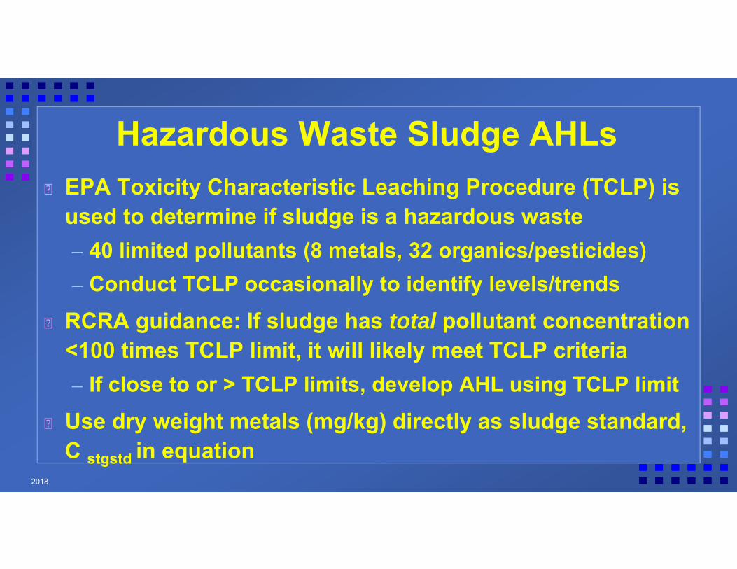
Hazardous Waste Sludge AHLsEPA Toxicity Characteristic Leaching Procedure (TCLP) is used to determine if sludge is a hazardous waste– 40 limited pollutants (8 metals, 32 organics/pesticides)– Conduct TCLP occasionally to identify levels/trends

RCRA guidance: If sludge has total pollutant concentration <100 times TCLP limit, it will likely meet TCLP criteria– If close to or > TCLP limits, develop AHL using TCLP limit

Use dry weight metals (mg/kg) directly as sludge standard, C stgstd in equation

•2018

Air Quality Based AHLsAHLair = AHL based air emission

standards, lbs/dayLinfl = POTW influent loading, lbs/dCairstnd = Air emissions standard, g/dayCair = Existing air emissions, g/dayRvol = Pollutant removal by volatilization (as decimal)0.0022 = Unit conversion factor

AHLs for Conventional PollutantsBOD, TSS and Ammonia– EPA recommends using the POTW’s rated average

design capacity plus any improvements as a “monthly average” based MAHL

Oil and Grease– 100 mg/l limit widely adopted for mineral or petroleum

O&G (Note: Basis is not site-specific/technical)– Level of animal FOG at which deposition in a sewer

pipe is negligible would be the basis for a collection system MAHL

•2018

Local limits should be established:– Where the average actual loading of a pollutant is

> 60% of the MAHL, or:– Where the maximum actual loading is > 80% of the

MAHL any time in the 12 month period preceding the analysis

– For BOD and TSS: Where the monthly average influent loading is > 80% of design capacity any one month in the 12 months before the headworks analysis

Actual Loading vs. MAHLsEPA Guidance

Determine Maximum Allowable Industrial Loading (MAIL)

MAHL MinusSafety FactorUncontrolled SourcesHauled WasteGrowth Factor

= MAIL



Alloc

ate A

llowa

ble In

dustr

ial Lo

ading

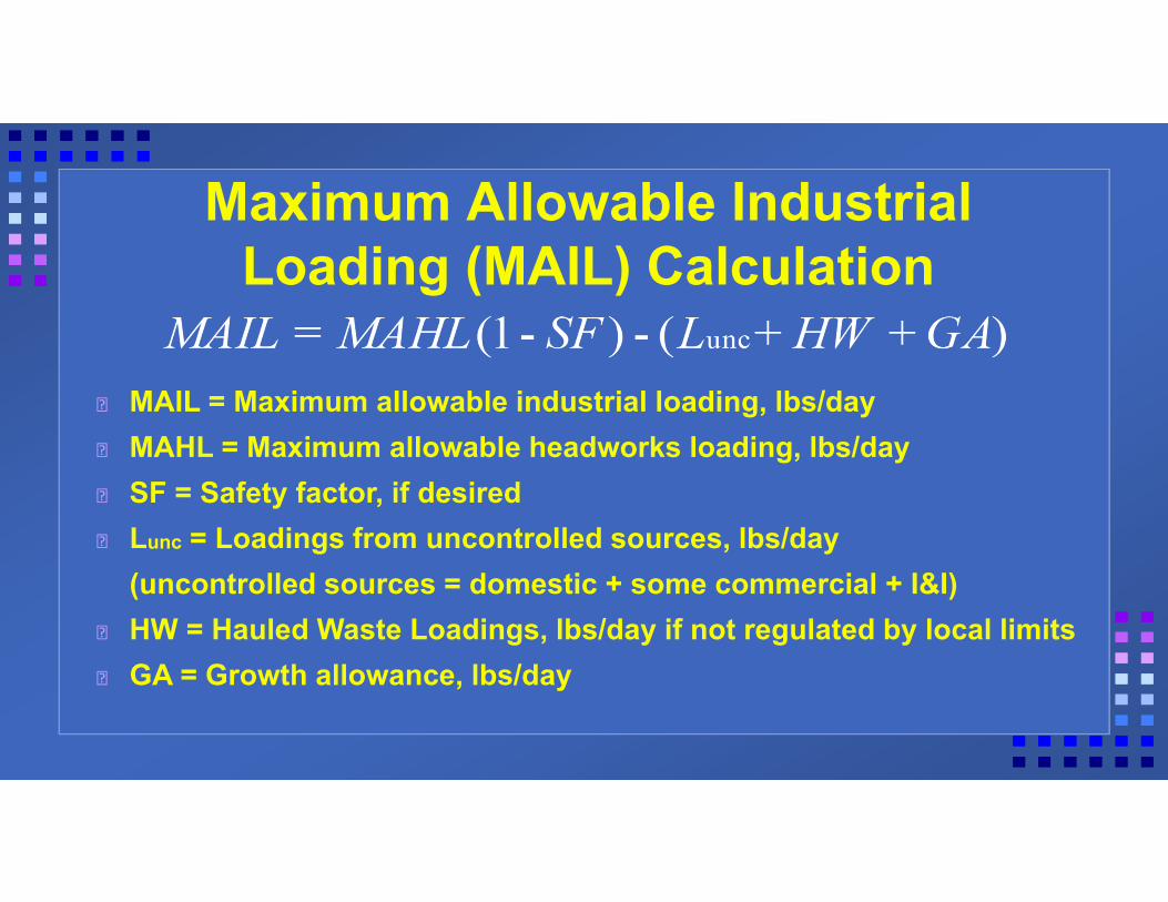
Maximum Allowable Industrial Loading (MAIL) Calculation

MAIL = Maximum allowable industrial loading, lbs/dayMAHL = Maximum allowable headworks loading, lbs/daySF = Safety factor, if desiredLunc = Loadings from uncontrolled sources, lbs/day(uncontrolled sources = domestic + some commercial + I&I)HW = Hauled Waste Loadings, lbs/day if not regulated by local limitsGA = Growth allowance, lbs/day

Safety FactorThe safety factor decision should consider:

The variability of the POTW’s dataThe amount of data the POTW used in its development of MAHLsThe quality of the POTW’s dataHow much literature data the POTW usedEPA recommends 10% Safety Factor

•2018

Safety Factor (continued)

The history of compliance with the parameter (both POTW and IUs)The potential for IU slug loadings (e.g., as a result of chemical spills)The number and size of each IU with respect to the POTW's flowCurrent Influent loading vs. Calculated MAHL

•2018

Uncontrolled SourcesDomestic usersSome or all of the commercial usersInflow and Infiltration [I&I]Storm water (if combined sewers)

– A minimum of at least 7 separate samples should be taken to assess variation in uncontrollable sources

– The number of sampling sites depends on the size of the collection system

Uncontrolled Loading Calculation

LUNC = Uncontrolled loading, lbs/dayCUNC = Uncontrolled pollutant concentration, mg/lQUNC = Uncontrolled flow, MGD8.34 = Unit conversion factor

QUNC = WWTP average flow (MGD) minus permitted SIU flow (MGD) which should be known for all SIUs (or use potable water use measurements).

Hauled WasteIf the POTW does not intend to regulate hauled wastes through local limits, the loading from these sources should be included with the uncontrolled sources.Should sample hauled wastes to insure that they:– are not hazardous– are not greater than expected (i.e., not greater

than background concentrations if treated as uncontrollable)

– will not pose risks to workers

Growth Allowance

If growth is anticipated, a portion of the MAHL should be reserved.Growth allowance is separate from a safety factorGrowth can come from new or expanding IUs, shopping malls, industrial parks, or new housing developmentsMost common for BOD, TSS, and other pollutants the POTW was designed to remove

THE HEADWORKS ANALYSIS1. Calculate the MAXIMUM ALLOWABLE HEAD-WORKS LOADING (MAHL) for each pollutant

2. Subtract a SAFETY FACTOR

3. Subtract UNCONTROLLABLE LOADING

5. Allocate MAXIMUM ALOWABLE INDUSTRIAL LOADING (MAIL) to Industrial Users

16.5 lbs Copper

10% = 1.65 lbs Copper 14.85 lbs Copper

8.35 lbs CopperPOTW

OK

4. Subtract a GROWTH FACTOR10%=1.65 lbs Copper 6.70 lbs Copper

6.5 lbs Copper

1. Uniform Concentration»Option 1. One limit for all POTWs»Option 2. Separate limits for each POTW

2. Industrial User Contributory Flow3. WYNIWYG4. Mass Proportional Limits5. Selected Industrial Reduction

Allocate MAIL to IUsCollect Data & Characterize Existing Loadings

Develop MAHLs


Alloc

ate A

llowa

ble In

dustr

ial Lo

ading

MAIL Allocation MethodsMAIL Allocation Method is very important decision made by Pretreatment Coordinator– Significant impacts on regulated community– Impacts on economic development of city

Method chosen should be “best fit” for POTW-specific (or pollutant specific) situation– Size of PT program, # of SIUs discharging a specific

pollutant, “size of the MAHL

Can More than One Method be Used?EPA does NOT dictate allocation methodAny allocation method can be selected as long as it is:

Protective, Enforceable, and Reasonable

One or more allocation methods can be used (different allocation methods for different pollutants)

Limit DurationDaily maximum

(most common)

Monthly average(permit based)

Instantaneous maximum(grab samples)

Allocation Approaches:1. Uniform Concentration

Same pollutant concentration limit applies to every controlled (permitted) discharger– Even those that do not discharge the pollutant

Method prevalent throughout most of the countryQuick and Easy!Calculation uses the pounds formula– Total flow of permitted dischargers in MGD, MAIL in

pounds, solve for mg/l

Allocation Approaches:Uniform Concentration

Limit (mg/l) = _____MAIL in POUNDS per Day__Total Controllable flow (MGD) x 8.34

Uniform Concentration AllocationMAIL = 11.01 pounds COPPER

TOTAL FLOW = 2.65 MGD

ALLOCATE ONE LIMIT BASED ON FLOW FROM ALL SIUs

= 11.01 lbs / (2.65 * 8.34) = 0.50 mg/l

0.265 MGD

0.529 MGD 0.265 MGD0.265 MGD 0.529 MGD

0.794 MGD

Uniform Concentration

COPPER LIMIT

POTW 2 POTW 1

POTW 3 POTW 4

1.43 mg/l 1.17 mg/l

2.14 mg/l 1.34 mg/l

1.17 mg/l

1.17 mg/l1.17 mg/l

OPTION 1ONE (MOST STRINGENT ) LIMIT

Option 1 AdvantagesNo economic advantages to any industryEasy to calculate and applyAllows for industrial growth in certain areas of the municipalityWastewater can be switched from one POTW to anotherSewer Use Ordinance contains limits that apply to ALL users


COPPER LIMIT

POTW 2 POTW 1

POTW 3 POTW 4

1.17 mg/l

POSSIBLE INDUSTRIAL EXPANSION

1.17 mg/l

1.17 mg/l1.17 mg/l

1 New Large Industry

6.5 New Large Industries 3.5 New Large Industries

No New Large Industry

Option 1 DisadvantagesLimits may be overly stringent for some industriesInflexible, no consideration given for actual POC dischargesOverprotection of the POTWPenalizes water conservationCan create unnecessary noncompliance


COPPER LIMIT

POTW 2 POTW 1

POTW 3 POTW 4

1.17 mg/l1.43 mg/l

1.34 mg/l2.14 mg/l

OPTION 2FOUR SEPARATE LIMITS

Uniform Concentration Option 2 Advantages

Better allocation of the different MAILsPOTWs not overprotectedLimits are fair to all SIUsEasy to calculate and apply

Option 2 DisadvantagesPOTW appears to grant economic advantages to industries in certain areas and penalize those in others

Enforcement problems arise if waste-water from one industry can be switched from one POTW to another

Option 2 DisadvantagesIndustrial Pretreatment Program more complex to administer with different limits for each pollutant

Minimal Industrial Growth Allowed

SUO complex or No Limits in SUO

•2018

Calculate pounds from non-contributing SIUs and subtract from MAIL (using uncontrollable mg/l)

Calculate total “contributory” flow from SIUs that discharge > uncontrollable/background levels

Divide MAIL by this flow

New concentration based limit applies ONLY to contributory SIUs

Allocation Approaches 2. Industrial User Contributory Flow

•2018

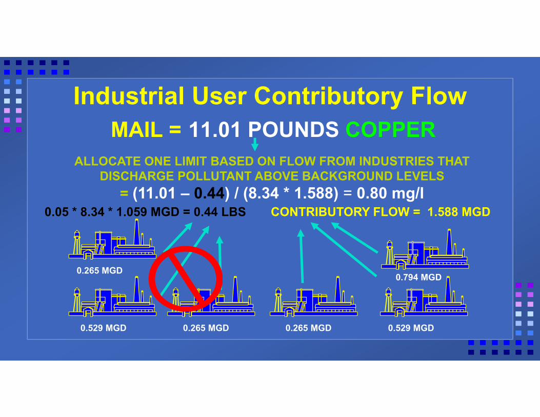
Industrial User Contributory FlowMAIL = 11.01 POUNDS COPPER

CONTRIBUTORY FLOW = 1.588 MGD

ALLOCATE ONE LIMIT BASED ON FLOW FROM INDUSTRIES THAT DISCHARGE POLLUTANT ABOVE BACKGROUND LEVELS

= (11.01 – 0.44) / (8.34 * 1.588) = 0.80 mg/l

0.265 MGD

0.529 MGD 0.265 MGD0.265 MGD 0.529 MGD

0.794 MGD

0.05 * 8.34 * 1.059 MGD = 0.44 LBS

Industrial User Contributory Flow

SIUs that discharge at or below the background level are given a background allocation

Sometimes a different allocation can be justified based on actual sample data

CLIM = Concentration limit for all users discharging a pollutant, mg/lLMAIL = MAIL, lbs/dayLBACK = Total background loading allocation for all users for which no contributory flow limit is being established for that pollutant, lbs/dayQCONT = Flow from all industrial and other controlled sources discharging the pollutant, MGD

AdvantagesCommon discharge limit established for all users identified as discharging a given pollutantMAIL apportioned more efficiently only to SIUs discharging the pollutant above background levelsLimits usually higher than uniform methodUnnecessary noncompliance reduced

Disadvantages

Need accurate flow and pollutant data for each SIUPenalizes water conservationSUO cannot contain limits

Cautions: Concentration Based Limits

Appears Fair on a Concentration Basis [Look at the pounds, though!]Be Careful…..– If your SIU develops an ambitious water

conservation program, they may “conserve” themselves right into noncompliance

– “I’d like a million gallons at that concentration, please…..”

Allocation Approaches3. What You Need is What You Get

WYNIWYGIU Limits Set on Case-by-Case Basis

Limits Can Be Based on:IU current loadingIU Ability to Pretreat Pollutants Other technically based factor

Limits: Concentration or Mass based

MAIL ALLOCATION METHODS:“W.Y.N.I.W.Y.G.”

“What You Need Is What You Get”Essentially a “pollutant trading” system with the POTW in complete control of the “trades”Permit Limit Determination– Review historical data– Determine limit/value that can be met

on a consistent basis– Add a “safety factor”

Uniform Concentration vs. WYNIWYG

TOTAL FLOW = 300,000 gpd

ALLOCATE ONE CONCENTRATION LIMIT BASED ON FLOW FROM ALL SIUs

= 2.5 pounds Nickel / (0.3 MGD * 8.34) = 1.0 mg/l

0.10 MGD 0.10 MGD 0.10 MGD

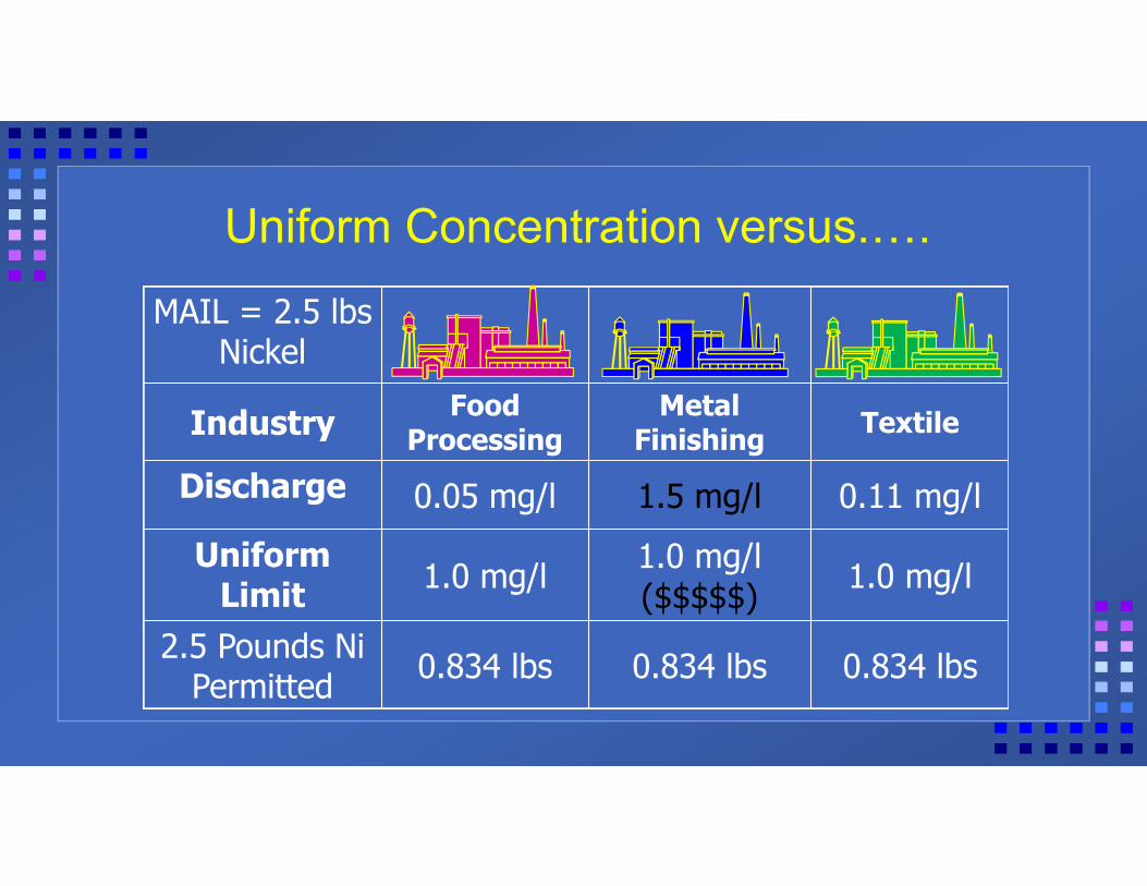
Uniform Concentration versus.….MAIL = 2.5 lbs

Nickel

Industry Food Processing

Metal Finishing Textile

Discharge 0.05 mg/l 1.5 mg/l 0.11 mg/lUniform

Limit 1.0 mg/l 1.0 mg/l ($$$$$) 1.0 mg/l

2.5 Pounds Ni Permitted 0.834 lbs 0.834 lbs 0.834 lbs

“What You Need Is What You Get”MAIL = 2.5 lbs

Nickel

Industry Food Processing

Metal Finishing Textile

Discharge 0.05 mg/l 1.5 mg/l 0.11 mg/lWYNIWYG

Limit 0.1 mg/l 2.38 mg/l (Categorical Std) 0.2 mg/l

2.23 Pounds Ni Permitted 0.08 lbs 1.98 lbs 0.17 lbs

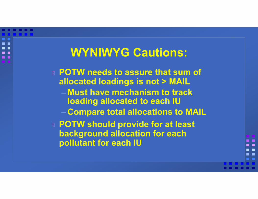
WYNIWYG Cautions:POTW needs to assure that sum of allocated loadings is not > MAIL– Must have mechanism to track

loading allocated to each IU– Compare total allocations to MAIL

POTW should provide for at least background allocation for each pollutant for each IU

WYNIWYG Allocation TableIncludes Limits and/or Background “Allocations” for each IU and pollutant Tracks POTW Loadings– SIU/IU Permitted Loadings– Uncontrollable [Domestic/Commercial]– Available MAHL/MAIL

Update Required with every new IU Permit/Permit Modification

AdvantagesMAIL apportioned more efficiently – Only to SIUs discharging pollutant above

background levels– No “unused” POTW capacity

Limits higher than uniform method– Avoids setting excessively stringent or

unachievable limitsProvides flexibilityUnnecessary noncompliance reduced

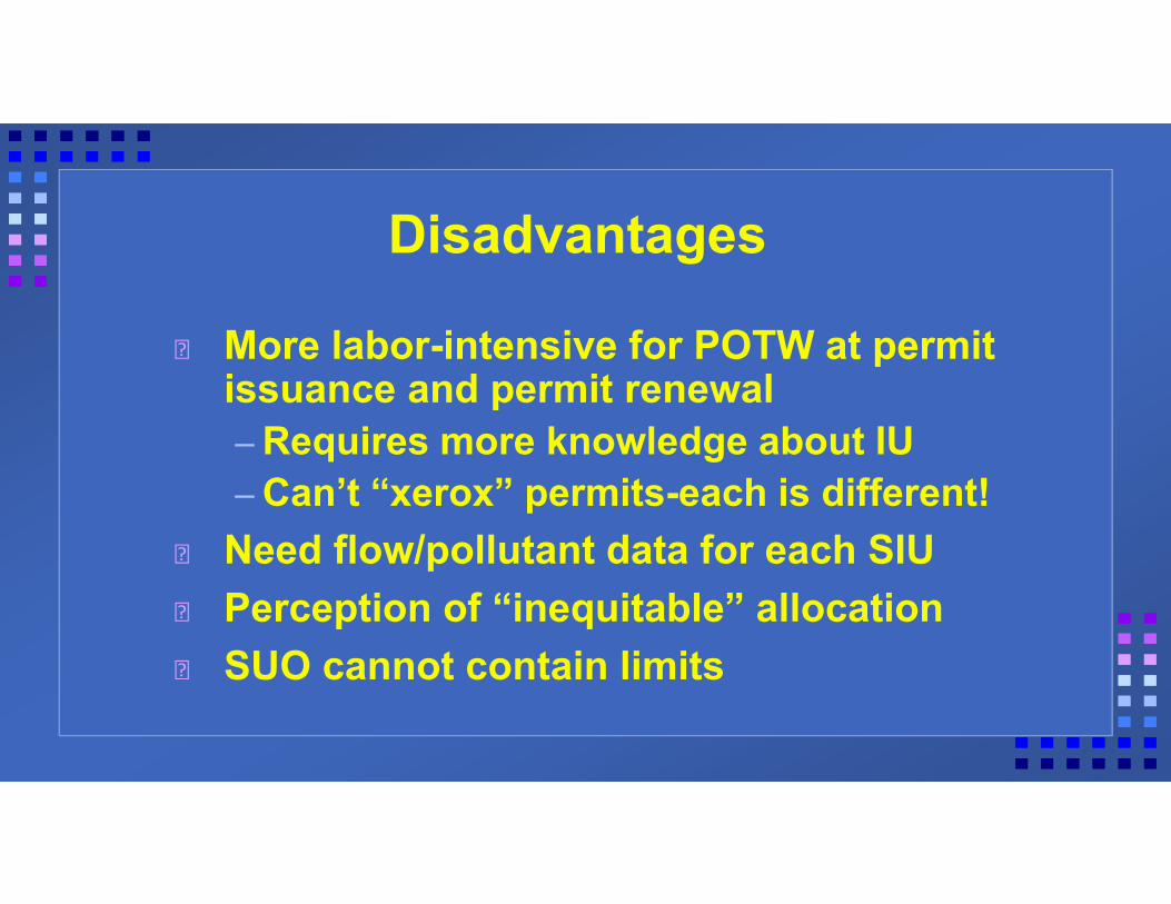
Disadvantages

More labor-intensive for POTW at permit issuance and permit renewal– Requires more knowledge about IU– Can’t “xerox” permits-each is different!Need flow/pollutant data for each SIUPerception of “inequitable” allocationSUO cannot contain limits

WYNIWYG AllocationsPROS

Equitable method for all SIUsMost representative of actual POTW capabilitiesReduces cost of compliance for most SIUsProperly administered, it is technically defensible

CONSComplicated method to administerRequires detailed tracking systemRequires detailed support documentation for allocationsCompliance evaluation is specific to individual permits

Allocation Approaches

4. Mass Proportional Limits

For each pollutant, allocate the MAIL as a different mass or concentration limit depending on each industrial user’s present mass discharge

Mass Proportional Formula

LALLx = Allowable loading allocated to user (lbs/day)LCURRx = Current loading from user (lbs/day)LCURRt = Total current loading to POTW from controlled sources in lbs/dayLMAIL = MAIL, lbs/dayLBACK = Total background loading allocation for all users for which no contributory flow limit is being established for that pollutant, lbs/day

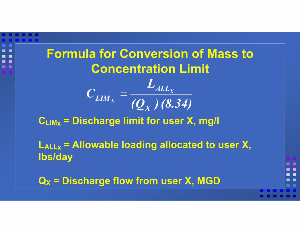
Formula for Conversion of Mass to Concentration Limit

CLIMx = Discharge limit for user X, mg/l

LALLx = Allowable loading allocated to user X, lbs/day

QX = Discharge flow from user X, MGD

Mass Proportion LimitsMAIL = 10 pounds

COPPER/DAY

ALLOCATE SEPARATE LIMITS TO EACH INDUSTRY BASED ON PRESENT LOADING OF EACH INDUSTRY X 10/8 (1.25)

= 1.25 TIMES0.794 MGD * 0.45 mg/l * 8.34 = 2.977 lbs

(0.5625 = 3.72 lbs)

ACTUAL LOADING = 8 pounds COPPER/DAY

0.529 MGD * 1.0 mg/l * 8.34 = 4.41 lbs (1.25 mg/l = 5.51 lbs)

0.265 MGD * 0.13 mg/l * 8.34 = 0.287 lbs (0.1625 mg/l = .3588 lbs)0.265 MGD * 0.048 mg/l * 8.34 = 0.106 lbs

(0.06 mg/l = 0.1325 lbs)

0.529 MGD *0.03 mg/l *8.34 = 0.132 lbs (0.0375 mg/l = 0.165 lbs)

0.265 MGD * 0.040 mg/l *8.34 = 0.088 lbs (0.050 mg/l = 0.11 lbs)

•2018

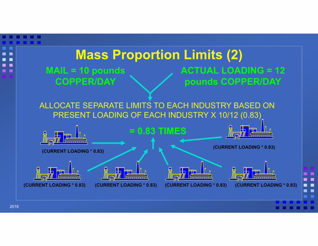
Mass Proportion Limits (2)MAIL = 10 pounds

COPPER/DAY

ALLOCATE SEPARATE LIMITS TO EACH INDUSTRY BASED ON PRESENT LOADING OF EACH INDUSTRY X 10/12 (0.83)

= 0.83 TIMES(CURRENT LOADING * 0.83)

ACTUAL LOADING = 12 pounds COPPER/DAY

(CURRENT LOADING * 0.83)(CURRENT LOADING * 0.83)(CURRENT LOADING * 0.83)(CURRENT LOADING * 0.83)

(CURRENT LOADING * 0.83)

•2018

AdvantagesLocal limits relate to SIUs present discharge rate Different limit derived for each pollutant for each SIU discharging that particular pollutantLimits may be expressed in permit as concentration or mass basedPromotes water conservation

DisadvantagesRequires detailed understanding of each user’s effluentMay penalize users that are presently pretreating their wastes when others are notLimits for new users are difficult to derive and have to be estimated at startup

Disadvantages 2No discharge limits put in the SUOIndustrial pretreatment program cumbersome due to individual limit calculations for all usersLimits may be difficult to implementExtra industrial user expense for flow monitoring equipment

Allocation Approaches5. Selected Industrial Reduction

Current headworks loading exceeds the MAIL for a particular pollutant

POTW requires selected SIUs to reduce their discharge of that pollutant on a case-by-case basis

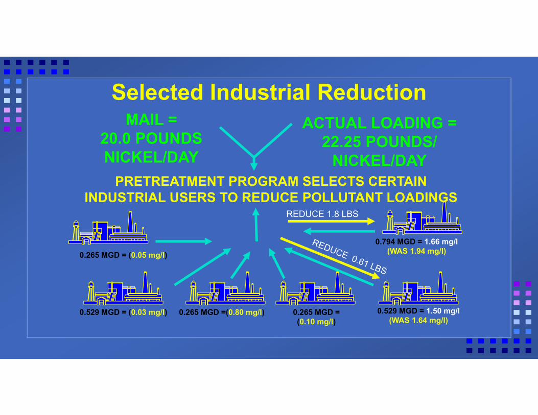
Selected Industrial ReductionMAIL =

20.0 POUNDS NICKEL/DAY

PRETREATMENT PROGRAM SELECTS CERTAIN INDUSTRIAL USERS TO REDUCE POLLUTANT LOADINGS

0.794 MGD = 1.66 mg/l(WAS 1.94 mg/l)

ACTUAL LOADING = 22.25 POUNDS/

NICKEL/DAY

0.529 MGD = 1.50 mg/l (WAS 1.64 mg/l)

0.265 MGD = (0.10 mg/l)

0.265 MGD =(0.80 mg/l)0.529 MGD = (0.03 mg/l)

0.265 MGD = (0.05 mg/l)

•REDUCE 1.8 LBS

AdvantagesMethod cost effectively reduces pollutant loadings by imposing reductions on only the significant dischargers of a pollutant on a case by case basisReductions based on wastewater treatability informationTechnology based limitations may be developed

AdvantagesPOTW focuses local limits strategy for a particular pollutant on selected industries for which available technology will bring about the greatest pollution abatement for the least amount of moneyAllows the POTW to identify similar industries and require them to achieve similar levels of pretreatment

POTW’s method for selecting industries for pollutant reduction will be subject to close examination and involvement by usersProceed with caution!The method requires a detailed under-standing of each user’s production processes and effluent constituents

Disadvantages

Disadvantages 2

Discharge limits cannot be put in the SUOIndustrial pretreatment program becomes cumbersome due to individual limit calculations for all usersExtra industrial user expense for flow monitoring equipment

Creative Allocation MethodsHampton Roads Sanitation District [VA]

Monthly Average Discharge Limitations in mg/l0 to

9,999 gpd

10,000 to 19,999

gpd

20,000 to 29,999

gpd

30,000 to 39,999

gpd

40,000 to 199,999

gpd

200,000 to 400,000

gpdCadmium 0.5 0.4 0.3 0.2 0.1 0.05Chromium 10.0 8.0 6.0 4.0 2.0 1.0Copper 10.0 8.0 6.0 4.0 2.0 1.0Lead 5.0 4.0 3.0 2.0 1.0 0.5Nickel 5.0 4.0 3.0 2.0 1.0 0.5Zinc 10.0 8.0 6.0 4.0 2.0 1.0Limits for SIUs >400,000 gpd are established on a case-by-case basis

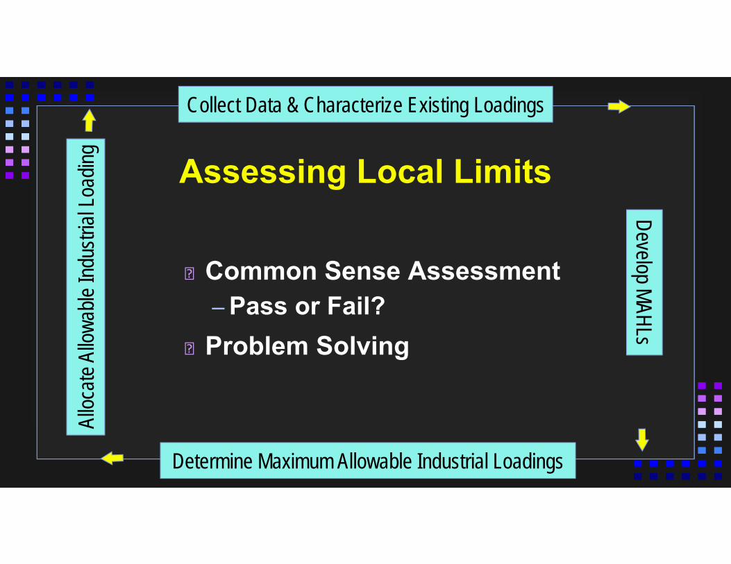
Assessing Local Limits

Common Sense Assessment– Pass or Fail?Problem Solving



Alloc

ate A

llowa

ble In

dustr

ial Lo

ading

Common Sense AssessmentAre the limits technologically achievable?

Can compliance with the limitsbe determined?Do the limits make sense based on actual POTW conditions and compliance experience?

Limits Fail Common Sense Test

Reassess development processCheck for correct environmental criteriaCheck removal ratesUncontrolled pollutant concentrationsLack of data and use of literature values Conduct additional sampling at lower

MDLs

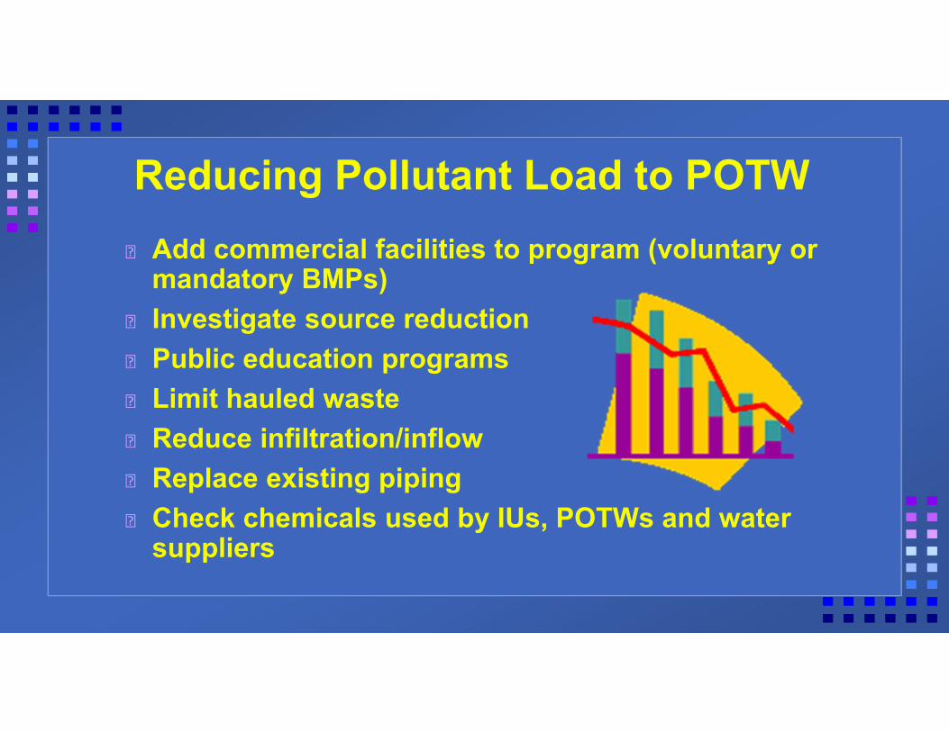
Reducing Pollutant Load to POTWAdd commercial facilities to program (voluntary or mandatory BMPs)Investigate source reductionPublic education programsLimit hauled wasteReduce infiltration/inflowReplace existing pipingCheck chemicals used by IUs, POTWs and water suppliers

Drastic Measures !!

Change sludge disposal methods

Expand POTW

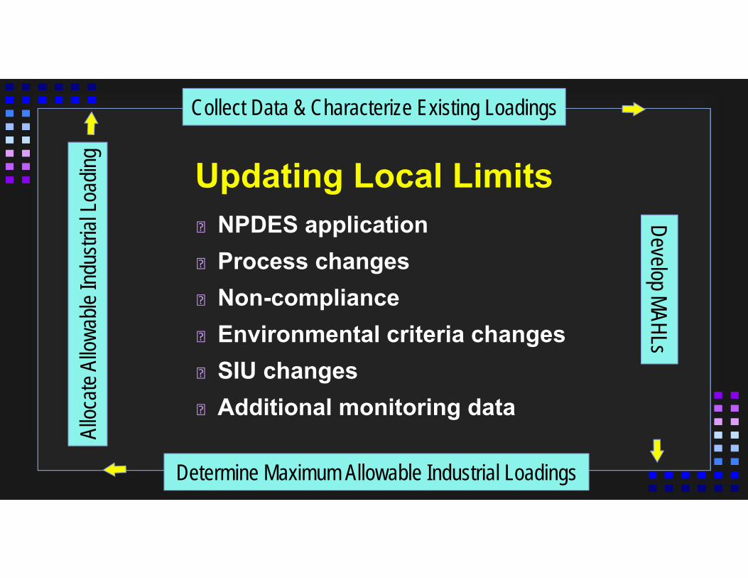
Updating Local LimitsNPDES applicationProcess changesNon-complianceEnvironmental criteria changesSIU changesAdditional monitoring data



Alloc

ate A

llowa

ble In

dustr

ial Lo

ading

NPDES Permit renewal/revisions40 CFR 122.44(j)(2)(ii) requires NPDES permit to contain a condition to provide a written technical evaluation of the need to revise local limits following permit re-issuance

Annual or detailed re-evaluation of local limits can meet this requirement

New or modified POTW or increased service areaPOTW process or operation significantly changedFlow significantly changedSludge disposal method changed

POTW Process Changes:

Review of Compliance History

Review compliance over past year to determine if Local Limits remain Protective of the POTW

If violations have occurred, take action against noncompliant SIUs, or develop new limits, or revise local limit concerned

New or revised NPDES limits

State water quality standards changed

Any other new data not available during the last local limits development effort

Environmental changes

New SIUs significantly change loadings

SIUs closed down

SIUs changed processes significantly

SIU Changes

+

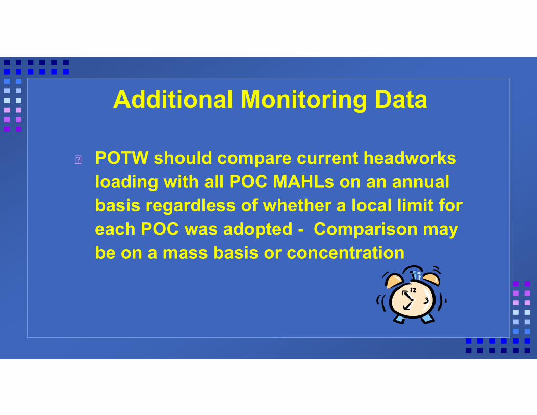
POTW should compare current headworks loading with all POC MAHLs on an annual basis regardless of whether a local limit for each POC was adopted - Comparison may be on a mass basis or concentration

Additional Monitoring Data

Comparison of Loading with MAHLs for Pollutants with no Developed Local Limit

Loading > MAHL Develop Limit for POC Investigate cause

Loading > threshold (first time)

Increase monitoring OR develop limit

Loading > threshold (second time)

Establish limit/increase monitoring

Loading < threshold Keep pollutant under review

IF THEN

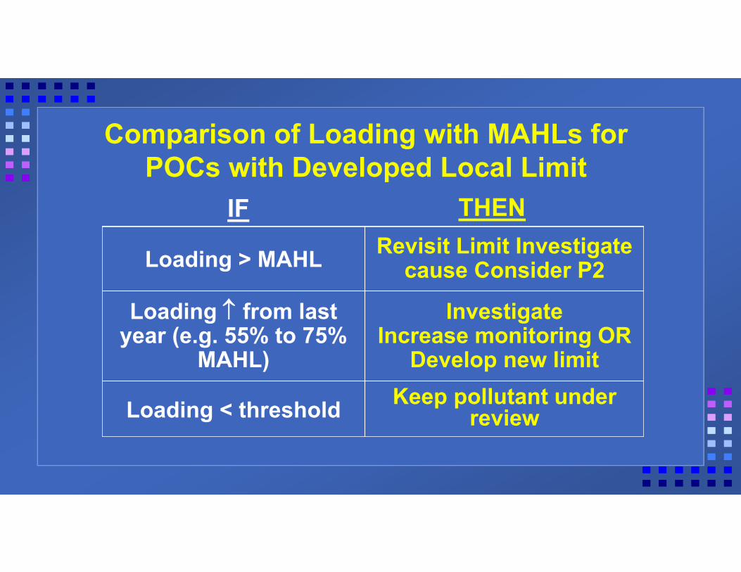
Comparison of Loading with MAHLs for POCs with Developed Local Limit

IF THEN

Loading > MAHL Revisit Limit Investigate cause Consider P2

Loading from last year (e.g. 55% to 75%

MAHL)

Investigate Increase monitoring OR

Develop new limit

Loading < threshold Keep pollutant under review

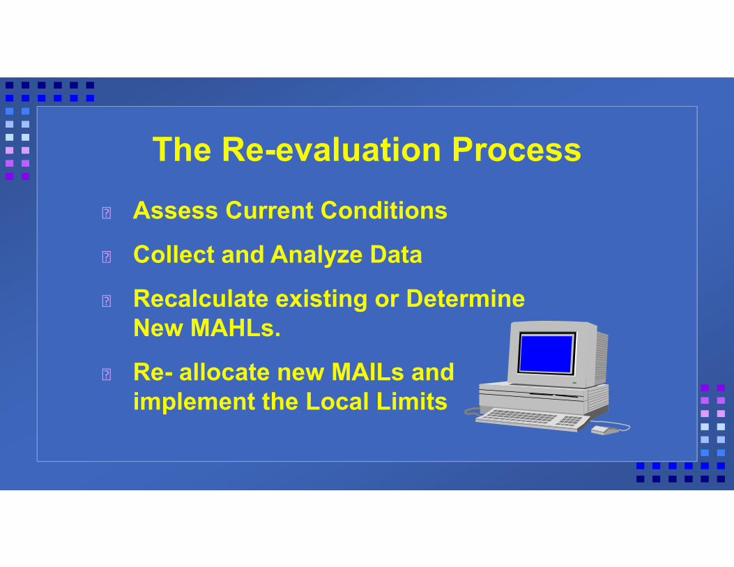
The Re-evaluation ProcessAssess Current Conditions

Collect and Analyze Data

Recalculate existing or Determine New MAHLs.

Re- allocate new MAILs and implement the Local Limits

Applying Local LimitsAdopt local limits into POTW Legal Authority [SUO]Include in individual IU Control Mechanism [SIU Permit]Combination of both



Alloc

ate A

llowa

ble In

dustr

ial Lo

ading

The most stringent limit

applies.

Questions???

industrial pretreatment advanced local limits

Documents