“industrial concentration, economic growth, and inequality
TRANSCRIPT

“Industrial Concentration,
Economic Growth, and Inequality
dynamics throughout the stages of
industrialisation: a comparative
and transnational analysis”
By Matteo Calabrese

1
Front picture from: https://www.toppr.com/guides/fundamentals-of-economics-cma
2
University of Leiden
2020
“Industrial Concentration, Economic Growth, and Inequality dynamics
throughout the stages of industrialisation: a comparative and transnational
analysis”
Research Master Thesis
Course: History (ResMA)
Specialisation: Cities, Migration, and Global Interdependence
By Matteo Calabrese
Student number: s2111365
Email: [email protected]
Thesis Supervisor: Prof.dr. Jeroen Touwen
Second Reader: Prof.dr. Catia Antunes

3
Table of Contents
1. Introduction ........................................................................................................................... 6
1.1. Research Question .......................................................................................................... 7
1.2. Thesis Structure and sub-research questions ................................................................. 8
1.3. Primary sources ............................................................................................................... 9
1.4. Methodology ................................................................................................................. 13
1.5. Theoretical Framework ................................................................................................. 15
PART I: Historical Insights from the Analysis of IPUMS Datasets
2. Historical patterns of GDP growth, household income inequality, and industrial
concentration: a bird-eye view ............................................................................................... 26
2.1 The United States ........................................................................................................... 28
2.2 Canada ............................................................................................................................ 30
2.3 Europe ............................................................................................................................ 33
2.3.1. The UK .................................................................................................................... 34
2.3.2. Spain ....................................................................................................................... 37
2.3.3. Italy ......................................................................................................................... 39
2.3.4. France ..................................................................................................................... 42
2.3.5. Germany ................................................................................................................. 45
2.4 The East-Asian miracle .................................................................................................. 46

4
2.4.1. Indonesia, Malaysia, Thailand ................................................................................ 47
2.5 China .............................................................................................................................. 49
2.6 South America ............................................................................................................... 52
2.6.1. Brazil ....................................................................................................................... 53
2.6.2. Argentina ................................................................................................................ 54
PART II: Theoretical Insights from the Analysis of IPUMS Datasets
3. Industrial Concentration in the Twentieth Century: industrialisation waves and reaction
to economic shocks ................................................................................................................. 59
3.`1. An “old” industrial revolution: East Asia and South America in comparison with the
US.......................................................................................................................................... 60
3.1.1. East Asian miracles ................................................................................................. 61
3.1.2. Thailand, China, and South American countries .................................................... 62
3.`2. The 1970s as a benchmark decade in the Western World: the beginning of a new
phase? .................................................................................................................................. 64
3.`3. Effects of economic shocks on the level of industrial concentration .......................... 65
4. Industrial Concentration in the Twentieth-First Century: where do we go from here? .. 68
4.1. Inversions of the industrial concentration trends catalysed by financial crises: the
2008 case .............................................................................................................................. 69
4.2. Future scenarios for industrial concentration: endogenous and exogenous shocks ... 70
4.3. Future research directions: industrial concentration and income inequality for African
countries ............................................................................................................................... 71

5
5. Conclusions .......................................................................................................................... 74
5.1. Societal Relevance ......................................................................................................... 75
6. Bibliography ......................................................................................................................... 77
7. Appendix .............................................................................................................................. 86
WORD COUNT: 29 348
WORD COUNT (without Table of Contents, footnotes, Bibliography, and Appendix): 20 225
6
1. INTRODUCTION
The impact of industrialisation on social inequality dynamics has been subject to
debate in many contexts. In academia but also at the policy-making level. Whereas the
relationship between economic growth and inequality has been investigated in numerous
studies 1 , very few have focused instead, on the role played by the level of industrial
concentration into this equation. The growth of GDP per capita can have a positive or negative
effect on the level of social inequality depending on the integrative leverage of a broad group
of variables: the initial wealth and geographic endowments2, the quality of institutions3, trade
and globalisation variables4, the growth rate of the population5, and so on. The level of
industrial concentration can be considered as part of this group of variables. On the one hand,
it gives a measure of the spatial transformation occurring throughout the stages of the
1 Cf. Klaus Deininger, and Lyn Squire, “A New Data Set Measuring Income Inequality,” World Bank Economic Review 10, no. 3 (September 1996): 565–591; Kristin J. Forbes, “A Reassessment of the Relationship between Inequality and Growth,” The American Economic Review 90, no. 4 (September 2000): 869-887; Orazio Attanasio, Pinelopi K. Goldberg, and Nina Pavcnikc, “Trade reforms and wage inequality in Colombia,” Journal of Development Economics 74 (August 2004): 331– 366; Abhijit V. Banerjee and Esther Duflo, “Inequality and Growth: What Can the Data Say?” Journal of Economic Growth 8 (June 2003): 267–99; Florence Jaumotte, Subir Lall, and Chris Papageorgiou, “Rising Income Inequality: Technology or trade and financial globalization?”, C. IMF Economic Review 61, no. 2 (April 2013): 271-309; Augustin K. Fosu, “Growth, Inequality and Poverty in Sub-Saharan Africa: Recent Progress in a Global Context,” Oxford Development Studies 43, no.1 (2015): 44-59. 2 Cf. William Easterly, “Inequality does cause underdevelopment: Insights from a new instrument,” Journal of Development Economics 84, (2007): 755–776.
3 Cf. Daron Acemoglu, Simon Johnson, and James A. Robinson, “The Rise of Europe: Atlantic Trade, Institutional Change, and Economic Growth,” American Economic Review 95, no. 3 (2005): 546-579. 4 Cf. Orazio Attanasio, Pinelopi K. Goldberg, and Nina Pavcnikc, “Trade reforms and wage inequality in Colombia,” Journal of Development Economics 74 (August 2004): 331– 366; Abhijit V. Banerjee and Esther Duflo, “Inequality and Growth: What Can the Data Say?” Journal of Economic Growth 8 (June 2003): 267–99; Florence Jaumotte, Subir Lall, and Chris Papageorgiou, “Rising Income Inequality: Technology or trade and financial globalization?”, C. IMF Economic Review 61, no. 2 (April 2013): 271-309. 5 Cf. Ayodele Odusola, Frederick Mugisha, Yemersrach Workie, and Wilmot Reeves, “Income Inequality and Population Growth in Africa,” UNDP Africa Reports 267039, United Nations Development Programme, 2017; Derek D. Heady, and Andrew Hodge, “The effect of population growth on economic growth: A meta-regression analysis of the macroeconomic literature,” Population and Development Review 35, no. 2 (June 2009):221-248; Tai-Hsin Huang, and Zixiong Xie, “Population and economic growth: A simultaneous equation perspective,” Applied Economics 45, (2013): 3820-3826.

7
industrialisation process. At the same time, in turn, endogenously affects both the level of
economic growth (by triggering forms of “circular causation” in the general demand6) and the
level of social inequality (through periphery-to-core migrations of populations7).
1.1 Research Question
The purpose of the present study is analysing the patterns of industrial concentration,
economic growth, and household income inequality through an integrative perspective. The
main research question analysed throughout the thesis is:
To what extent is it possible to prospect a relationship between these three variables?
The countries subject of the research are chosen based on their significance in the light of the
critiques to the Kuznets’ hypothesis and secondly, on their availability in the main primary
source used in the present research: the IPUMS International collection of historical census
datasets. They can be ultimately divided in three major groups:
a) the US, Canada, the UK, and part of the Western countries analysed by Midelfart-Knarvik
et al.8 (Italy, France, Germany, and Spain). For this group, the time range analysed is from
1860 to 2011.
b) the group of Latin American countries, with Argentina and Brazil. This group is analysed in
order to evaluate the critique of Deinenger and Squire9 to Kuznets’ theory and since the two
countries available in the dataset were “new-comers” to industrialisation in the 1960s10. The
time range here analysed, due to the IPUMS datasets availability, is 1960-2000.
6 Cf. Paul Krugman, “Increasing returns and economic geography,” Journal of Political Economy 99, no. 3 (June 1991): 483 – 499. 7 Cf. Simon Kuznets, “Economic Growth and Income Inequality,” American Economic Review 45, no.1 (March 1955): 1–28. 8 Karen Helene Midelfart-Knarvik, Henry G. Overman, Stephen J. Redding, and Anthony J. Venables, “The Location of European Industry,” report for the European Commission, 2000. 9 Klaus Deininger, and Lyn Squire, “A New Data Set Measuring Income Inequality,” World Bank Economic Review 10, no. 3 (September 1996): 565–91, p.259. 10 Cf. Alan Gilbert, and David Goodman, “Regional income disparities and economic development: a critique”, in Development Planning and Spatial Structure, ed. Alan Gilbert (London, 1976), 113-141; Belen Barroeta, Javier Gómez, Prieto Jonatan, and Paton Manuel Palazuelos, “Innovation and Regional Specialisation in Latin America Identifying conceptual relations with the EU Smart Specialisation
8
c) The group of available new industrialising countries in East and South-East Asia: China,
Thailand, Malaysia, and Indonesia. This group is analysed in order to evaluate the critique of
the World Bank Report of 199311 to Kuznets’ theory. The time range analysed is from 1970 to
2000.
1.2 Thesis structure and sub-research questions
The research is organised as follows:
Firstly, an introductive chapter with an analysis of the primary sources used, a discussion on
the methodology, and a literature review about the relationship between industrial
specialisation, economic growth, and inequality.
Chapter 2 is dedicated to a historical analysis of the trends of industrial concentration and
income inequality. Two main sub-research questions will be assessed:
- Is it possible to find common paths of development among the countries object of the
research, based on the analysis of the trends for industrial concentration and income
inequality throughout the Twentieth Century?
- Does industrial concentration for Europe have an upturn during the 1970s, consistently with
Milanovic’s theory on a second Kuznets’ wave starting in those years?
Chapter 3 contains theoretical insights that can be derived from my analysis of the industrial
concentration and income inequality series for the Twentieth Century. Again, two sub-
research questions are analysed:
- Are the 1970s the beginning of a new Kuznets’ wave for the Western world (despite declining
levels of industrial concentration)?
approach,“ technical report by the Joint Research Centre (JRC), the European Commission’s science and knowledge service, 2017.
11 Nancy M. Birdsall, Jose E. L. Campos, Chang-Shik Kim, W. Max Corden, Lawrence Mac Donald, Howard Pack, John Page, Richard Sabor, and Joseph E. Stiglitz, “The East Asian miracle : economic growth and public policy : Main report (English),” World Bank policy research report, 1993.

9
- How to explain on the one hand, the quick reduction of the levels of industrial concentration
after the Second World War, and on the other, the either increasing or decreasing value of
the Krugman Index concurrently with economic and financial crises?
Chapter 4 is dedicated to the implications that the analysis of the industrial concentration and
income inequality series for the Twentieth Century has for future scenarios in the Twenty-
First Century. I discuss in the first place, the possibility of an inversion of the industrial
concentration trend, starting from the 2010s. Secondly, I analyse the possible effects of the
economic shock related to the Covid-19 pandemic on the values for industrial concentration
in the 2020 decade. Finally, I focus on possible research directions for the analysis of the
industrialisation development in sub Saharan Africa (SSA) countries, between the 1990s and
the 2010s.
The conclusions summarise my results and prospect related policy implications.
1.3. Primary Sources
The primary sources used in the present research are in the first place, census data.
The IPUMS Center has made available a group of sample datasets for 98 countries12, derived
from census surveys starting from the 1960s (sometimes with historical sections from
previous years) and collected every ten years until the 2010s. All the original census data
have been stratified and harmonised by the Centre. In this way, on the one hand the original
composition of the population has been preserved albeit subject to the sampling process –
namely, the sample is not taken in a random way: the basic data topology is maintained and
mirrored throughout the sample13. On the other, the variables related to the characteristics
of the individuals surveyed (from the type of assets owned to the industry in which they are
employed) are conveyed to standard categories, making therefore easier the work for
12 The aggregated census datasets from the IPUMS International online archive can be found at https://international.ipums.org/international/Minnesota Population Center. Integrated Public Use Microdata Series, International: Version 7.2 [dataset]. Minneapolis, MN: IPUMS, 2019. https://doi.org/10.18128/D020.V7.2 13 Furthermore, the samples are still quite big: from 900 000 individuals to 10 000 000.
10
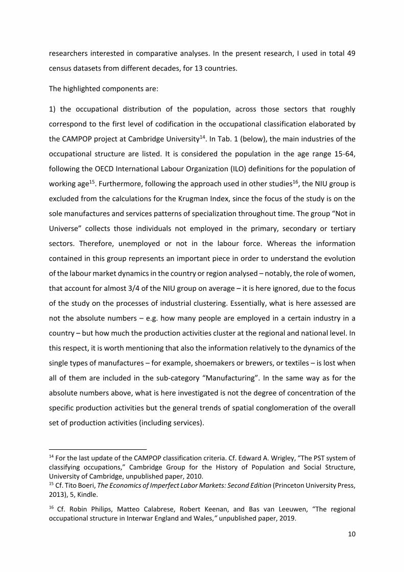
researchers interested in comparative analyses. In the present research, I used in total 49
census datasets from different decades, for 13 countries.
The highlighted components are:
1) the occupational distribution of the population, across those sectors that roughly
correspond to the first level of codification in the occupational classification elaborated by
the CAMPOP project at Cambridge University14. In Tab. 1 (below), the main industries of the
occupational structure are listed. It is considered the population in the age range 15-64,
following the OECD International Labour Organization (ILO) definitions for the population of
working age15. Furthermore, following the approach used in other studies16, the NIU group is
excluded from the calculations for the Krugman Index, since the focus of the study is on the
sole manufactures and services patterns of specialization throughout time. The group “Not in
Universe” collects those individuals not employed in the primary, secondary or tertiary
sectors. Therefore, unemployed or not in the labour force. Whereas the information
contained in this group represents an important piece in order to understand the evolution
of the labour market dynamics in the country or region analysed – notably, the role of women,
that account for almost 3/4 of the NIU group on average – it is here ignored, due to the focus
of the study on the processes of industrial clustering. Essentially, what is here assessed are
not the absolute numbers – e.g. how many people are employed in a certain industry in a
country – but how much the production activities cluster at the regional and national level. In
this respect, it is worth mentioning that also the information relatively to the dynamics of the
single types of manufactures – for example, shoemakers or brewers, or textiles – is lost when
all of them are included in the sub-category “Manufacturing”. In the same way as for the
absolute numbers above, what is here investigated is not the degree of concentration of the
specific production activities but the general trends of spatial conglomeration of the overall
set of production activities (including services).
14 For the last update of the CAMPOP classification criteria. Cf. Edward A. Wrigley, “The PST system of classifying occupations,” Cambridge Group for the History of Population and Social Structure, University of Cambridge, unpublished paper, 2010. 15 Cf. Tito Boeri, The Economics of Imperfect Labor Markets: Second Edition (Princeton University Press, 2013), 5, Kindle.
16 Cf. Robin Philips, Matteo Calabrese, Robert Keenan, and Bas van Leeuwen, “The regional occupational structure in Interwar England and Wales,” unpublished paper, 2019.

11
Tab. 1. Occupational structure format for all the countries analysed. Source: IPUMS, 2020
2) The geographical unit, that roughly corresponds to the NUTS1 (Nomenclature of Territorial
Units for Statistics) level. The NUTS system is the standard for statistical surveys as defined by
Eurostat and adopted by the European Union. This system gives a hierarchical subdivision of
the economic territory of the EU. NUTS1 is the level of “major socio-economic regions” (see
https://ec.europa.eu/eurostat/web/nuts/background).
The major limitations in the use of IPUMS as a primary source lie in the first place, in the fact
that not all the countries have the same availability of datasets throughout the years. Notably,
a lack of data for the years after the 2000s is common to many of the countries analysed.
Secondly, an inner characteristic of the census data collections should also be considered as
a factor to be carefully assessed throughout the analysis. Census surveys are usually
NIU (not in universe) Private household services
Agriculture, fishing, and forestry Financial services and insurance
Mining Public administration and defense
Manufacturing Real estate and business services
Electricity, gas and water Education
Construction Health and social work
Wholesale and retail trade Other services
Hotels and restaurants Unknown
Transportation, storage and communicati

12
implemented every ten years, and typically during the first or the second year of the decade.
For this reason, the societal picture emerging from each census survey should be more
correctly considered as being directly affected by the events and the governmental policies
of the prior decade. For example, the result I obtain for the Argentinian degree of industrial
concentration in 1990, must be linked to the governmental policies of the 1980s and not to
those of the following decade. The outcome of the policies and economic events that
occurred in the 1990s is instead reflected in the value which I found for the year 2000.
GDP per capita data are extracted from the harmonised historical series of GDP data
of the Maddison Project Database at
https://www.rug.nl/ggdc/historicaldevelopment/maddison/releases/maddison-project-
database-2018. GINI coefficients for the historical series of the US and the UK are derived
from Milanovic’s reconstruction of these series17. GDP growth data and GINI coefficients for
the years after the 1960s are derived from the World Bank datasets
( https://data.worldbank.org/) and the Clio-Infra database (https://clio-infra.eu/)
Whereas the major limitations of the Maddison Database are well known – namely, the fact
that all the figures of the pre-industrial era should be considered as estimates, due to the lack
of reliable statistical data for those years18– a more thorough explanation should be devoted
to the choice of the GINI coefficient as an indicator of the level of inequality for the societies
object of the research.
The GINI coefficient is a proxy number for the actual level of equality in the distribution of
income and wealth in each country here assessed. Many other measures of income inequality
and poverty have been proposed throughout the years: from the relative mean variation to
the 80/20, 90/10, 95/5 ratios19 for the measurement of income inequality, to the head-count
17 Branko Milanovic, “The inequality possibility frontier: the extensions and new appliacations,” Comparative Institutional Analysis Working Paper Series 13, (2013):1-28. 18 Cf. Thomas Piketty, Capital in the twenty-first century (Belknap Press of Harvard University Press, 2014); Branko Milanovic, Global inequality: a new approach for the age of globalization (Cambridge, Massachusetts: Harvard University Press, 2016). 19 These ratios evaluate the differences in income distribution between the percentiles of the population. For example, the 90/50 gives the distance between the top deciles and the middle ones;

13
ratio and the aggregate poverty gap for a quantification of the level of poverty20. Piketty21 has
extensively argued the insufficiency of the GINI coefficient as a global indicator of the wealth
distribution within and between nations. In effect, the GINI coefficient, calibrated solely on
income inequalities, gives only a part of the picture. The gains on yields and rents of the
resurging “society of rentiers” do not enter in the GINI mathematical relation.
Despite the soundness of these observations, in the present study, it will be nevertheless still
used the GINI coefficient for the following reasons: a) like the Krugman-Index (discussed in
the next paragraph) and on the contrary of the relative mean variation, it respects the “Pigou–
Dalton Principle of Transfers”22; b) on the contrary of the percentiles and deciles ratios and of
the poverty measurement, it gives (despite some loss of information, especially in the
confrontation between the top and middle percentiles and deciles) a measure that can be
more easily used as a harmonised index in the comparison between low, middle and high
income countries; c) the World Bank and the other publications of the countries here analysed
adopt the GINI coefficient. Summing up: although it does not fully describe the whole body
of relations and issues relative to the wealth and income distribution, it is an effective and
immediate proxy for it.
1.4. Methodology
The work of Krugman on trade theory and economic geography23 has introduced a
model able to integrate comparative advantage and geographical endowment factors to
the 99/90, gives the distance between the highest percentiles and the high ones (see for example, https://www.equalitytrust.org.uk/how-economic-inequality-defined ) 20 For a more extensive discussion on these indexes: Jean Hindriks, and Gareth D. Myles, Intermediate Public Economics (MIT Press, 2013), Kindle.
21 Thomas Piketty, Capital in the twenty-first century (Belknap Press of Harvard University Press, 2014) 22 Namely that “the inequality index decreases if there is a transfer of income from a richer household to a poorer household that preserves the ranking of the two households in the income distribution and leaves the total income unchanged” (Jean Hindriks, and Gareth D. Myles, Intermediate Public Economics (MIT Press, 2013), 470, Kindle. 23 Cf. Paul Krugman, “Increasing returns and economic geography,” Journal of Political Economy 99, no. 3 (June 1991): 483 – 499; Paul Krugman, "The Myth of Asia's Miracle," Foreign Affairs 73, (November/December 1994): 62-78; Paul Krugman and Anthony J. Venables, “The Seamless World: A
14
“path-dependence”24 factors (such as the evolution of transportation costs and forms of
circular causation of demand).
In Krugman’s model, the above-mentioned elements are eventually combined in a coherent
formulation including a) variations in the transportation costs, b) scale economies and spill-
overs benefits (e.g.: Marshallian externalities, pecuniary and non-pecuniary externalities; c)
the variation of the demand linked to processes of “circular causation” - namely, when “other
things equal, it will be more desirable to live and produce near a concentration of
manufacturing production because it will then be less expensive to buy the goods this central
place provides [..] Manufactures production will tend to concentrate where there is a large
market, but the market will be large where manufactures production is concentrated”25.
In the present study, I will derive the index of specialisation, named after him, to assess firstly
the level of regional specialisation and then, from the average of the regional values, the
country level of specialisation, being the latter the main variable of interest. Many of the
studies focusing on industrial concentration have used Krugman-type indexes26. The Krugman
Spatial Model of International Specialization,” Centre for Economic Policy Research, Discussion Paper, no. 1230, 1995. 24 Path dependence is in the definition of David a “dynamic process whose evolution is governed by its own history “ (Paul. A. David, “Path dependence: a foundational concept for historical social science,” Cliometrica 1, no. 2 (May 2007): 91 – 114, p. 91). For other applications of a path dependency approach to economic geography studies cf. Nicholas Crafts, and Nikolaus Wolf, “The Location of the UK Cotton Textiles Industry in 1838: A Quantitative Analysis,” The Journal of Economic History 74, no.4 (December 2014): 1103-1139; Stefan Nikolic, “Determinants of industrial location: Kingdom of Yugoslavia in the interwar period,” European Review of Economic History 22, no. 1, (February 2018): 101–13.
25” Paul Krugman, “Increasing returns and economic geography,” Journal of Political Economy 99, no. 3 (June 1991): 483 – 499, p. 486. 26 Cf. Sukkoo Kim, “Economic Integration and Convergence: U.S. Regions, 1840–1990,” Journal of Economic History 58, no. 3 (April 1998): 659–683; Karen Helene Midelfart-Knarvik, Henry G. Overman, Stephen J. Redding, and Anthony J. Venables, “The Location of European Industry,” report for the European Commission, 2000; Nicholas Crafts, and Abay Mulatu, “What explains the location of industry in Britain, 1871–1931?”, Journal of Economic Geography 5, no. 4 (August 2005): 499-518; Thor Berger, Kerstin Enflo, and Martin Henning, “Geographical location and urbanisation of the Swedish manufacturing industry, 1900–1960: evidence from a new database,” Scandinavian Economic History Review 60, no.3 (November 2012): 290-308; Anna Missiaia, “The industrial geography of Italy: provinces, regions and border effects (1871–1911)” (PhD diss., London School of Economics, 2015), Chapter 2; Stefan Nikolic, “Determinants of industrial location: Kingdom of Yugoslavia in the interwar period,” European Review of Economic History 22, no. 1, (February 2018): 101–13; Robin Philips, Matteo Calabrese, Robert Keenan, and Bas van Leeuwen, “The regional occupational structure in Interwar England and Wales,” unpublished paper, 2019.
15
Index respects indeed a series of criteria that make it a reliable indicator: the principle of
“enforced anonymity” ensures that the resulting degree of specialization is the same for
different permutations of the same employment share. The ‘Pigou-Dalton Principle’ ensures
equity of allocation throughout the rankings 27 . Moreover, this index offers a further
advantage: since it is the most used index for this type of analyses, a work of comparison
between the previous studies and the present one is therefore facilitated.
The index is calculated as follows:
𝐾𝑆𝐼𝑟 = ∑ 𝐴𝐵𝑆 ( 𝑠𝑟,𝑖𝑖 − 𝑠𝑖) (1)
where 𝑠𝑟,𝑖 is the share of sector i of total employment in region r and 𝑠𝑖 is the share of sector
i in the overall country (in the same way as a standard deviation of the values of the sectors
per region from the average values of the country). The numerical value of the specialization
index ranges from 0, in the case that the regions have an identical sector structure compared
to the national structure, to 2, in which the sector structure is completely different across
regions.
1.5 Theoretical framework
Already in Kuznets’ theory, the spatial transformation of the industrial tissue is one of
the primary factors on the basis of the strict relationship that he individuates between
economic growth (GDP per Capita growth) and the level of income inequality. Migrations from
the “agricultural periphery” towards the “industrialized core”– as in the definition of
Krugman 28 – have a profound effect on the overall income distribution. The household
incomes of the agricultural population are typically smaller than the urban ones and have a
27 Cf. Nicole Palan, “Measurement of Specialization – The Choice of Indices,” FIW Working Paper N° 62, 2010. 28 Paul Krugman, “Increasing returns and economic geography,” Journal of Political Economy 99, no. 3 (June 1991): 483 – 499, p.485.
16
more equal distribution. For Kuznets, therefore, “first, [..] the increasing weight of urban
population means an increasing share for the more unequal of the two component
distributions. Second, the relative difference in per capita income between the rural and
urban populations does not necessarily drift downward in the process of economic growth”29.
Subsequent studies by Williamson 30, Lindert and Williamson 31, Harris and Todaro32 , Rauch33,
and Kim34 have gone further in this path, by hypothesising a relation between the level of the
industrial concentration and the so-called “Kuznets curve” alongside the overall cycle of the
economic development. In Kuznets’ curve, the level of household income inequality first
raises and then, after reaching a peak, drops while the development of the country (GDP per
capita) goes forward – in the characteristic inverted U-shaped form. In the same way, the
level of industrial concentration follows a similar pattern. In the initial phases of the
industrialization, the tendency towards geographical conglomeration of the manufactures
increases. Afterwards, throughout the successive stages of the development, the distribution
of the industries becomes more diversified. Thus, the values for industrial concentration
become smaller and smaller.
A complete negation of the findings and research approach of Williamson has been proposed
by Krebs. Starting from the considerations of Therkildsen35 on the biases of the empirical
method of Williamson – based on the calculation of the spatial inequality through a coefficient
of variation – he finds that “the paradigm of converging regional disparities does not meet
with strong support from recent data. The patterns of regional development in less-
29 Simon Kuznets, “Economic Growth and Income Inequality,” American Economic Review 45, no.1 (March 1955): 1–28, p. 7-8. 30 Jeffrey Williamson, “Regional Inequality and the Process of National Development: A Description of the Patterns,” Economic Development and Cultural Change 13, (1964): 3–84.
31 Peter Lindert, and Jeffrey Williamson, “Growth, Equality and History,” Explorations in Economic History 22, (1985): 341–77. 32 John R. Harris, and Michael P. Todaro., “Migration, Unemployment and Development: Two-Sector Analysis,” American Economic Review 60, no. 1 (1970): 126–42. 33 James E. Rauch, “Economic Development, Urban Underemployment, and Income Inequality,” Canadian Journal of Economics 26, no. 4 (November 1993): 901–18. 34 Cf. Sukkoo Kim, “Economic Integration and Convergence: U.S. Regions, 1840–1990,” Journal of Economic History 58, no. 3 (April 1998): 659–83; Sukkoo Kim, “Spatial Inequality and Economic Development: Theories, Facts, and Policies,” working Paper n. 16, 2008. 35 Ole Therkildsen, “The relationship between economic growth and regional inequality: a critical reappraisal,” paper presented at the Fourth Advanced Studies Institute in Regional Science Siegen, 1978.
17
developed countries indicate just the opposite of a stabilizing spatial transformation. In
industrialized countries hardly any significant convergence of the regional income level can
be observed, though the degree of spatial concentration and the gap between high and low-
income regions is considerably less” 36.
Many studies, though, have afterwards empirically demonstrated the existence of that type
of bell-shaped curve for industrial concentration, throughout the stages of the
industrialisation process. Kim, for example, obtains a Williamson-type pattern of industrial
concentration alongside the curve of economic development of the US, between the second
half of the Nineteenth Century and the Twentieth37. The US, during this time frame, became
indeed more and more de-specialised, concurrently with the growth of the services sector38.
Tirado et al.39 and Betran40 find for Spain, in a consistent comparison with the US values found
by Kim, increasing values of industrial concentration in the second half of the Nineteenth
Century, and then a bell-shaped pattern with a peak in the Interwar years and a descending
curve afterwards in the Twentieth. For Italy, Missaia41 and Daniele et al.42 find the same
pattern with very high values of regional concentration in the early industrialization phases
before the 1900 (even though Daniele et al. obtain smaller values compared to Missaia), and
then the usual pattern decreasing after the wars until the 2000s. For England, the works of
36 Gunter Krebs, “Regional Inequalities during the Process of National Economic Development: A Critical Approach,” Geoforum 13, no. 2 (December 1982): 71-81. 37 Cf. Sukkoo Kim, “Economic Integration and Convergence: U.S. Regions, 1840–1990,” Journal of Economic History 58, no. 3 (April 1998): 659–83; Sukkoo Kim, “Spatial Inequality and Economic Development: Theories, Facts, and Policies,” working Paper n. 16, 2008. 38 Ibid., p.15 39 Daniel A. Tirado, Elisenda Paluzie, and Jordi Pons, “Economic Integration and Industrial Location: The Case of Spain before World War I,” Journal of Economic Geography 2, no.3 (July 2002):343–63. 40 Concha Betran, “Regional specialisation and industry location in the long run: Spain in the US mirror (1856–2002),” Cliometrica 5, no. 3 (October 2011): 259-290. 41 Anna Missiaia, “The industrial geography of Italy: provinces, regions and border effects (1871–1911)” (PhD diss., London School of Economics, 2015). 42 Vittorio Daniele, Paolo Malanima, Nicola Ostuni, “Unequal Development. Geography and Market Potential in Italian Industrialisation 1871-2001,” Regional Science Association Journal 97, no.3 (August 2018): 639-662.
18
Lee43 firstly, and then of Crafts and Mulatu44 as well as Philips et al. 45 show again the bell
pattern with a peak in the Interwar years. Philips46 for Belgium and Netherlands, and Berger,
Enflo, and Henning 47 for Sweden confirm also for these countries the same bell-shaped
pattern with a peak in the Interwar years. Finally, Midelfart-Knarvik et al. 48 have then
investigated the pattern for industrial concentration for the whole Europe, from an integrated
perspective. Their results show for Europe, when compared to the U.S, lower levels of
regional specialisation in absolute values. Furthermore, and more importantly, on the
contrary of the US (from Kim’s results), their pattern is increasing from the late 1980s.
Extending the glaze towards the other contexts of interest for the present research, Gilbert
and Goodman49 find for Brazil increasing levels of spatial concentration for industries and
population, starting from the 1940s (also due to the external and internal migration flows).
At the same time, despite a growth of the income per capita, the level of inequalities was
growing as well50. Azzoni et al.51 find that regional spatial inequality started to decline from
the 1980s (until 1997, last year they check for). In the same years, in Argentina, Barroeta et
al.52 find that a process of regional de-specialisation was ongoing in the long run despite the
43 Cf. John C. H. Lee, British Regional Employment Statistics, 1841-1971 (Cambridge: Cambridge University Press, 1979). 44 Cf. Nicholas Crafts, and Abay Mulatu, “What explains the location of industry in Britain, 1871–1931?”, Journal of Economic Geography 5, no. 4 (August 2005): 499-518
45 Cf. Robin Philips, Matteo Calabrese, Robert Keenan, and Bas van Leeuwen, “The regional occupational structure in Interwar England and Wales,” unpublished paper, 2019.
46 Cf. Robin Philips, “Continuity or Change? The Evolution in the Location of Industry in the Netherlands and Belgium (1820 – 2010)”, (PhD diss., Amsterdam University, 2020). 47 Cf. Thor Berger, Kerstin Enflo, and Martin Henning, “Geographical location and urbanisation of the Swedish manufacturing industry, 1900–1960: evidence from a new database,” Scandinavian Economic History Review 60, no.3 (November 2012): 290-308. 48 Cf. Karen Helene Midelfart-Knarvik, Henry G. Overman, Stephen J. Redding, and Anthony J. Venables, “The Location of European Industry,” report for the European Commission, 2000.
49 Cf. Alan Gilbert, and David Goodman, “Regional income disparities and economic development: a critique”, in Development Planning and Spatial Structure, ed. Alan Gilbert (London, 1976), 113-141. 50 Ibid., p.129 51 Cf. Carlos Azzoni, Naercio Menezes-Filho, and Taitane Menezes, “Opening the Convergence Black Box: Measurement Problems and Demographic Aspects,” in Spatial Inequality and Development, eds. R. Kanbur and A.J. Venables (Oxford: Oxford University Press, 2005). 52 Belen Barroeta, Javier Gómez, Prieto Jonatan, and Paton Manuel Palazuelos, “Innovation and Regional Specialisation in Latin America Identifying conceptual relations with the EU Smart Specialisation approach,“ technical report by the Joint Research Centre (JRC), the European Commission’s science and knowledge service, 2017, p. 26.
19
contrasting action of governmental policies in the 1980s and in the 1990s. Tambunan53 for
Indonesia and Ying54 for China find an empirical correlation between high concentration of
regional economic activity and development gaps between East-Asian regions after the 1960s.
Focusing on China, Hu55 individuates in the foreign trade another factor interfering in the
relationship between industrial concentration and development dynamics. Nakajima et al.56
empirically demonstrate for Indonesia (in the time span 1980-2000) that the initial
distribution of input factors has the major role in the future industrial concentration
outcomes. For Malaysia, Roslan57 finds decreasing levels of inter-regional spatial inequality
between 1970-1990 as well as reducing levels of household income inequalities. For Thailand,
Kittiprapas 58 , and Pansuwan 59 find the same trend for industrial clustering: increasing
between 1960-1980; declining between the 1990s and 2000s.
The above mentioned studies for the US, the UK, Spain, and Italy, focusing on the long run,
have found this common pattern: a curve that grows throughout the first decades of the
Twentieth Century, reaches a peak in the interwar years, and then descends in the second
part of the century.
53 Tulus T.H. Tambunan, Industrialization in Developing Countries: The Case of Indonesia (Industrialisasi di Negara Sedang Berkembang: Kasus Indonesia) (Jakarta: Indonesian-Ghalia, 2001). 54 Ge Ying, “Regional Inequality, Industry Agglomeration and Foreign Trade: The Case of China,” research Paper No. 105, 2006. 55 Dapeng Hu, “Trade, Rural-Urban Migration, and Regional Income Disparity in Developing Countries: A Spatial General Equilibrium Model Inspired by the Case of China,” Regional Science and Urban Economics 32, no. 3 (May 2002): 311-38. 56 Kentaro Nakajima, Yukiko Saito, and Iichiro Uesugi, “Measuring Economic Localization: Evidence from Japanese Firm-Level Data: Design of Inter Firm Network to Achieve Sustainable Economic Growth,” Working Paper Series No. 10, 2012. 57 Cf. Harhap A.H.Roslan, “Income Distribution and the Changing Tolerance towards Inequality in Malaysia – A Case of Hirschman’s Tunnel Effect?”, paper presented at the University of Wales Economics Colloquium on the 8-10 June 2000; Harhap A.H. Roslan, “Income Inequality, Poverty and Development Policy in Malaysia,” paper presented at the International Seminar on "Poverty and Sustainable Development", 22 & 23 November 2001. 58 Sauwalak Kittiprapas, "Regional concentration and the location behavior of manufacturing firms in the electronics and automobile industries in Thailand," Dissertations available from ProQuest,1995. 59 Cf. Apisek Pansuwan, “Regional Specialization and Industrial Concentration in Thailand, 1996-2005. Indonesian,” Journal of Geography 41, no.1 (June 2009): 1-17; Apisek Pansuwan, “Industrial Decentralization Policies and Industrialization in Thailand,” Silpakorn University International Journal 9, n.10 (August 2010): 117-147.

20
The bells described in these curves, though, tend to have a series of oscillations that make the
trend less smooth.
Graph 1. Historical Krugman Index series for Industrial Concentration for US, UK, Spain, Italy,
and Europe.
Source: Kim (1995); Betran (2011); Daniele et al. (2013); Crafts and Mulatu (2005); Midelfart-Knarvik
et al. (2000).
In the first place, as it is visible in the graph above, the figures for the industrial concentration
typically have an increase between the end of 1800. Then, after an initial decrease during the
first two decades of 1900 (see the US and the UK), a new increase in the Interwar years, and
finally a decreasing after the wars (see in particular, the values found by Crafts and Mulatu
0
0,2
0,4
0,6
0,8
1
1,2
1 8 6 0 1 8 8 0 1 8 9 0 1 9 0 0 1 9 1 0 1 9 2 0 1 9 3 0 1 9 4 0 1 9 5 0 1 9 6 0 1 9 7 0 1 9 8 0 1 9 9 0 2 0 0 0
INDUSTRIAL CONCENTRATION VALUES IN LITERATURE
United States (Kim)
Spain (Tirado et al; Betran)
Uk (Crafts and Mulatu; Philips et al., Martin et al.)
Midelfart-Knarvik (2000)

21
for Britain 60 , Kim for the US 61 , and Betran for Spain 62 ). This perturbation can partially
invalidate the idea of a perfect overlapping of the industrial concentration trend with the
Kuznets curve, as it was originally conceived. However, this divergence in the trends should
be linked with one of the most criticised aspects of Kuznets’ theory (see for example, among
the others, Piketty63, and Milanovic64). Namely, that Kuznets “essentially ignores the roles of
wars”65. The endogenous shock caused by wars – I follow here the theory of Milanovic about
the endogenous character of this type of shock, in partial contrast with Piketty66– affects all
the variables of interest in this research. As suggested by Milanovic, wars must be included in
a Kuznets-type framework, since “wars can lead to declines in inequality but also,
unfortunately, and more importantly, to declines in mean incomes”67.
Secondly, as it is visible in the comparison in Graph 1 between the trend found for the US by
Kim and the trend found for Europe by Midelfart-Knarvik et al.68, industrial concentration,
that is typically descendent in the second part of 1900, has instead for Europe an upturn in
the 1970s. Again, the deviation from the original Kuznets curve can be reconsidered in the
light of the critiques of Kuznets’ hypothesis. In many quarters69 have been indeed raised
doubts about the real effectivity of his curve as a predictor of the level of income inequalities
60 Nicholas Crafts, and Abay Mulatu, “What explains the location of industry in Britain, 1871–1931?”, Journal of Economic Geography 5, no. 4 (August 2005): 499-518
61 Cf. Sukkoo Kim, “Economic Integration and Convergence: U.S. Regions, 1840–1990,” Journal of Economic History 58, no. 3 (April 1998): 659–83; Sukkoo Kim, “Spatial Inequality and Economic Development: Theories, Facts, and Policies,” working paper n. 16, 2008. 62 Concha Betran, “Regional specialisation and industry location in the long run: Spain in the US mirror (1856–2002),” Cliometrica 5, no. 3 (October 2011): 259-290. 63 Thomas Piketty, Capital in the twenty-first century (Belknap Press of Harvard University Press, 2014). 64 Branko Milanovic, Global inequality: a new approach for the age of globalization (Cambridge, Massachusetts: Harvard University Press, 2016). 65 Ibid., p.98. 66 Cf. Thomas Piketty, Capital et idéologie (Le Seuil, Kindle Edition). Here Piketty has then analysed the endogenous nature of revolutions and class upheavals. 67 Branko Milanovic, Global inequality: a new approach for the age of globalization (Cambridge, Massachusetts: Harvard University Press, 2016), p. 5 68 Karen Helene Midelfart-Knarvik, Henry G. Overman, Stephen J. Redding, and Anthony J. Venables, “The Location of European Industry,” report for the European Commission, 2000. 69 Cf. Thomas Piketty, Capital in the twenty-first century (Belknap Press of Harvard University Press, 2014); Kristin J. Forbes, “A Reassessment of the Relationship between Inequality and Growth”, The American Economic Review 90, no. 4 (September 2000): 869-887; William Easterly, “Inequality does cause underdevelopment: Insights from a new instrument,” Journal of Development Economics 84, (2007): 755–776; Michael Kremer, “Population Growth and Technological Change: One Million B.C. to 1990,” The Quarterly Journal of Economics 108, no. 3 (August 1993): 681-716.

22
in correlation with the level of economic development. Among the others, Deininger and
Squire70 find no proof for the Kuznets’s relation between inequality and economic growth,
after empirically testing a wide panel sample of countries. A famous World Bank Report from
199371, furthermore, brought to the general attention the fact that a group of East-Asian
countries – Japan, South Korea, Taiwan, Hong Kong, Singapore, Thailand, Malaysia, and
Indonesia – between the 1960s and the 1990s, followed a completely different pattern (than
the one prospected by Kuznets) in their transformation towards fully industrialised countries.
Whereas these East-Asian economies were rapidly increasing, the inequality numbers were
kept somehow low, thanks to peculiar macroeconomics policies issued in combination with
land reforms and investments in human capital endowment72.
The upturn of the inequality level during the 1970s in the Western world has been extensively
analysed by Piketty 73 and Milanovic 74 . The societies that had become industrialised
throughout the first half of the Twentieth Century (or before) should have been, at that point,
on the right (descending) branch of the Kuznets curve. Inequality was instead on the rise.
Piketty explains the failure of Kuznets’ formulation, by defining it as the product of a sort of
history accident. For him, inequalities went down during the Twentieth Century mainly due
to the exogenous shocks of the two World Wars. The U-turn from the 1970s should be
therefore seen as the beginning of a return to “normality”. Namely, to a society where the
wealth divide is made stable by high capital returns. Milanovic, on the other hand, presents
another explanation. Whereas “Piketty’s ideas explain the trajectory of inequality in the
United States and the United Kingdom over almost one hundred years from the early
twentieth to the early twenty-first century, […] if we extend our gaze further back, into the
eighteenth and nineteenth centuries, we see an increase in inequality that Piketty’s theory
does not explain”75. For this reason, Milanovic elaborates the concept of “Kuznets wave”, able
70 Klaus Deininger, and Lyn Squire, “A New Data Set Measuring Income Inequality,” World Bank Economic Review 10, no. 3 (September 1996): 565–591.
71 Nancy M. Birdsall, Jose E. L. Campos, Chang-Shik Kim, W. Max Corden, Lawrence Mac Donald, Howard Pack, John Page, Richard Sabor, and Joseph E. Stiglitz, “The East Asian miracle : economic growth and public policy : Main report (English)”, World Bank policy research report, 1993. 72 Ibid. 73 Thomas Piketty, Capital in the twenty-first century (Belknap Press of Harvard University Press, 2014) 74 Branko Milanovic, Global inequality: a new approach for the age of globalization (Cambridge, Massachusetts: Harvard University Press, 2016), p. 5. 75 Ibid., p.48

23
to give a more encompassing explanation to the oscillations of the inequality level around a
fixed average income level in the pre-industrial world, to its drop after the two world wars,
and finally to the rising inequality after the 1970s:
“In a nutshell, for the period before the Industrial Revolution, I argue that inequality moved in
Kuznets waves undulating around a basically fixed average income level. […] Second, after the
Industrial Revolution, inequality and mean income entered into a relationship that was absent
before, when the mean income was fixed. I argue that a structural change (movement into a
much more diversified manufacturing sector) and urbanization, along the lines proposed by
Kuznets, drove inequality up starting from the time of the Industrial Revolution to a peak in
the rich countries which occurred at the end of the nineteenth century or the beginning of the
twentieth. […] The forces that drove inequality down after World War I had come to an end
by the 1980s, the period around which we date the beginning of the second Kuznets curve for
the rich countries. The 1980s ushered in a new (second) technological revolution,
characterized by remarkable changes in information technology, globalization, and the rising
importance of heterogeneous jobs in the service sector. This revolution, like the Industrial
Revolution of the early nineteenth century, widened income disparities”76
The oscillations of the inequality level – and therefore the consequent structure of the
Kuznets waves – are triggered by two types of forces: “benign”, such as “technological change
that favours low-skilled workers” or “widespread education”; or “malign”, such as wars,
revolutions, epidemics77. Both types of forces can potentially reduce inequalities and must be
necessarily considered together when discussing the relationship between economic growth
and social inequality throughout history.
76 Ibid., p.53-55 77 Ibid., p.56
24
PART I
HISTORICAL INSIGHTS FROM THE ANALYSIS OF IPUMS DATASETS

25
In the hardest working part of Coketown; in the innermost fortifications of that ugly citadel, where Nature was
as strongly bricked out as killing airs and gases were bricked in; at the heart of the labyrinth of narrow courts
upon courts, and close streets upon streets, which had come into existence piecemeal, every piece in a violent
hurry for some one man’s purpose, and the whole an unnatural family, shouldering, and trampling, and
pressing one another to death; in the last close nook of this great exhausted receiver, where the chimneys, for
want of air to make a draught, were built in an immense variety of stunted and crooked shapes, as though
every house put out a sign of the kind of people who might be expected to be born in it.
Charles Dickens, Hard Times, Chapter X
Electricity was used sparingly to save money, and most dinners were eaten in near-darkness. There was no
plumbing and no heating. In the wet chill of a Hubei winter, the whole family wore their coats and gloves
indoors, and the cement walls and floors soaked up the cold like a sponge. If you sat too long, your toes went
numb, and your fingers too; the best remedy was to drink a cup of hot water, holding it with your hands while
the steam warmed your face. The children often watched television standing up, jumping up and down to
restore feeling in their toes.
Leslie T. Chang, Factory Girls. From Village to a City in a Changing China

26
2. Historical patterns of GDP growth,
household income inequality, and
industrial concentration: a bird-eye view
As a premise to the following analysis, it is important to stress that the Krugman Index
values are not inherently bad or good. This number does not immediately represent the state
of development of a country. Neither it is a measure of the level of industrialisation. More
correctly, it is a geographical measure of the level of dispersion of all the industries that are
operational throughout the regions of a country at a given time. For example, Spain in 1860
and Argentina in 1970 have the same value of industrial concentration at the country level –
namely: 0.44, see Tab. 2 and Tab.5 in the Appendix. This equivalence, though, is just about
the level of spatial disaggregation of all the industries (from the primary sector to the services)
in the national territory.
In this sense, the pre-industrialised world and the current service-based economies tend to
be, paradoxically, rather similar. Lower levels of industrial concentration – and, therefore, of
industrial specialisation78 – can be found for example for rural societies in the early years of
their industrialisation take-off, as well as for high-income countries during the first decades
of the Twentieth Century. The similarity, though, is just in the absolute values of the index.
The low levels of industrial concentration that I find for example for the Us, Canada, the UK,
Spain, Italy, France, and Germany between the second half of 1900 and 2010s, reveal indeed
78 Industrial concentration and industrial specialisation at the region and then country level can in effect be considered as specular concepts: “regional specialisation expresses the territorial perspective and depicts the distribution of the shares of the economic activities in a certain region, usually compared to the rest of the country, while geographic concentration of a specific economic activity reflects the distribution of its regional shares” (Zizi Goschin, Daniela L. Constantin, Monica Roman, and Bogdan Ileanu, “Specialisation and Concentration Patterns in the Romanian Economy,” Journal of Applied Quantitative Methods 4, no.1, (Spring 2009): 95-111, p.100).

27
in the first place, the constant growth of the third sector within these economies – throughout
their transformation in service-based economies79 . The service industry is indeed for its
inherent nature more dispersed and less dependent from geographical endowments than the
others. Secondly, a generalised reduction of transportation costs and an increase of
congestion costs. As pointed out by Daniele et al., during this phase of the industrialisation
process, industrial concentration eventually decreases also due to “location diseconomies
and congestion costs [that] work as centripetal forces and [due to] technical know-out
spreading” 80.
The pursuing of industrial strategies based on scale economies is therefore, at this stage,
progressively less common. People employed in the third sector are dislocated more
uniformly all over the country’s territory. The regional occupational structure becomes more
similar to the national one. The industrial apparel of these countries, throughout its three
sectors, ultimately assumes a full-fledged national dimension, abandoning the patchy
regional or city-based production structure.
Does the modification of the spatial characterisation of the industrial tissue also determine
variations of the household income inequality levels in the countries analysed?
As mentioned above, the Kuznets’ formulation has a strong spatial component. There is in
effect, evidence for many of the countries object of this research of a parallel movement of
the two trends. Concurrently with the progressive growth of the GDP per capita, inequalities
raise during the take-off of the industrialisation wave and its first phases. Then progressively
follow the same descending path as for the industrial concentration level. This trend is
observable until the 1970s for the Western high-income countries and until the 2000s for the
Latin-American and East-Asian countries here analysed. From these benchmark points, the
two trends diverge.
79 Gary Akehurst, and Jean Gadrey, The Economics of Services (London: Frank Cass, 1989). 80 Vittorio Daniele, Paolo Malanima, Nicola Ostuni, “Unequal Development. Geography and Market Potential in Italian Industrialisation 1871-2001,” Regional Science Association Journal 97, no.3 (August 2018): 639-662, p. 9.
28
2.1. The United States
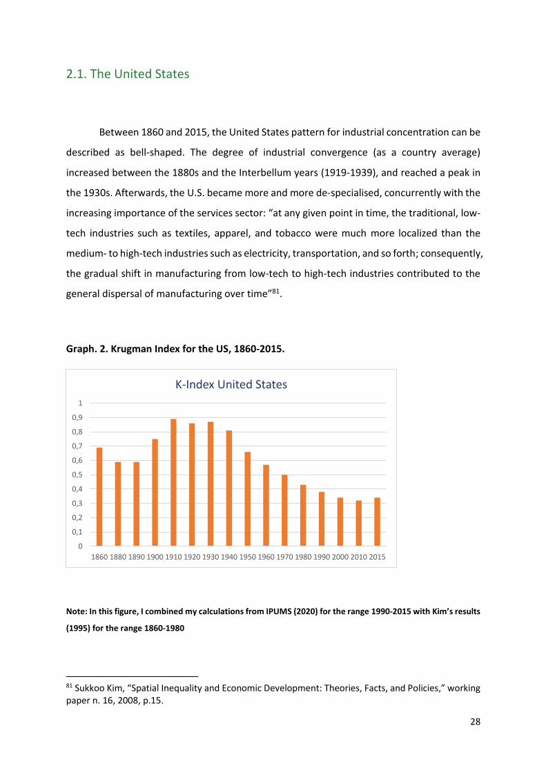
Between 1860 and 2015, the United States pattern for industrial concentration can be
described as bell-shaped. The degree of industrial convergence (as a country average)
increased between the 1880s and the Interbellum years (1919-1939), and reached a peak in
the 1930s. Afterwards, the U.S. became more and more de-specialised, concurrently with the
increasing importance of the services sector: “at any given point in time, the traditional, low-
tech industries such as textiles, apparel, and tobacco were much more localized than the
medium- to high-tech industries such as electricity, transportation, and so forth; consequently,
the gradual shift in manufacturing from low-tech to high-tech industries contributed to the
general dispersal of manufacturing over time”81.
Graph. 2. Krugman Index for the US, 1860-2015.
Note: In this figure, I combined my calculations from IPUMS (2020) for the range 1990-2015 with Kim’s results
(1995) for the range 1860-1980
81 Sukkoo Kim, “Spatial Inequality and Economic Development: Theories, Facts, and Policies,” working paper n. 16, 2008, p.15.
0
0,1
0,2
0,3
0,4
0,5
0,6
0,7
0,8
0,9
1
1860 1880 1890 1900 1910 1920 1930 1940 1950 1960 1970 1980 1990 2000 2010 2015
K-Index United States

29
The values for industrial concentration decreased after the 1860s. Significantly, after the end
of the Civil War – likely indicating a flattening of the industrial differences between the states
of the South and of the North. Furthermore, as argued by Kim, “the integration of U. S. regions
proceeded rapidly after 1860. The national railroad mileage in operation increased sharply
from 30,626 to 166,703 miles between 1860 and 1890. In 1860 railroads were regional
systems often with their own particular track gauges-there were at least seven different track
gauges in operation with sizes ranging from 4'3" to 6'0". But by 1890 most railroad lines had
converted their tracks to a standard gauge of 4'8.5"82 .
Essentially, following Krugman’s theoretical framework, from the 1860s until the 1890s, the
transportation costs continuously decreased. As a consequence, de-specialisation trends
were fostered. At the same time though, concurrently with the United States going between
1860 to 1914 “from being a predominantly agrarian economy to being the leading industrial
producer in the world”83, the emergence of economies of scale and the growing importance
of localised resource endowments determined an acceleration towards regional industrial
specialisation dynamics. Industrial specialisation reached thus a first peak in the 1910s, and
then decreased starting from the 1920s – even though, concurrently with the crisis of 1929,
it gained again some momentum. However, from the 1940s the level of industrial
concentration has been then decreasing without interruptions until the 2010s. The inversion
in the trend from the 1940s, can be again framed in the context of Krugman’s theorisation:
“as factors became increasingly more mobile and as technological innovations favoured the
development of substitutes, recycling, and less resource-intensive methods over the
twentieth century, regional resource differences diminished. The growing similarity of
regional factor endowments and the fall in scale economies caused regions to become de-
specialised between World War II and today”84.
82 Sukkoo Kim, “Economic Integration and Convergence: U.S. Regions, 1840–1990,” Journal of Economic History 58, no. 3 (April 1998): 659–83; p.885.
83 Ibid., p.896 84 Ibid., p. 902

30
The household income inequality level85, at the same time, followed a very similar pattern.
The (first) Kuznets’ wave for the US reached a peak firstly around the 1860s and then, after a
reduction, again in 1933. Afterwards, the curve was descending until the 1970s86. Basically,
the industrial concentration trend followed the Kuznets’ curve. From the 1970s, the GINI
coefficient had instead a divergent trend: whereas industrial concentration was still declining,
the household income inequality level began to increase87. The two patterns maintain their
directions until the period ranging between 2010 and 2015. In these years, immediately after
the financial crisis of 2008, there was a progressive increase of the percentage weight, within
the national occupational structure, of the financial service and of the business service sectors.
The former went from 4.44% in the 2000s to 4.47% in the 2010s. The latter went instead from
6.96% in the 2000s to 12.08 % in the 2010s. These increments did not have a clear reflection
in the industrial concetration value at the country level for the 2010, which once again
confirmed the descending trend. Nevertheless, the trend of industrial concentration that had
been continuosly decreasing for the US since the Interwar years, suddenly had an upturn in
the year 2015. In Chapter 4, I will analyse this value within my interpretation of the temporary
increases of the industrial concentration, resulting from the adoption of scale economies
policies at the firm and country level as a response to conjunctural economic crises.
2.2. Canada
As mentioned in the introduction, the trend for industrial concentration found by
Midelfart-Knarvik et al. 88 for Europe (see Tab. 3 in the Appendix) is convergent with the trend
of income inequality between 1980 and 1990. Whereas the US have a continuously
descending trend for industrial concentration in the time range 1940-2010, for Canada I find
an upturn as well in the 1980s. Therefore, in the same benchmark decade as for Midelfart-
85 Based on Milanovic’s calculations in Branko Milanovic, “The inequality possibility frontier: the extensions and new appliacations,” Comparative Institutional Analysis Working Paper Series 13, (2013). 86 Ibid., p.10
87 See graph 3 in the Appendix. 88 Karen Helene Midelfart-Knarvik, Henry G. Overman, Stephen J. Redding, and Anthony J. Venables, “The Location of European Industry,” report for the European Commission, 2000, p. 472.
31
Knarvik et al. (see Tab. 4 in the Appendix). Nevertheless, from the 1990s, the figures become
again decreasing until 2011. In Chapter 3, I will argue that this temporary inversion of the
trend for Canada can be in principle associated to the effect of the oil crisis of 1973 on
productive strategies at the country and firm level.
Canada, in the time range analysed, 1971-2011, became progressively more integrated with
the extra-US markets. In the same way as for many South American economies throughout
those years89 (see also the paragraph on Brazil below), tariffs on trade were increasingly cut.
Under the umbrella of the General Agreement on Tariffs and Trade (GATT) – outcome of the
“Tokyo Rounds” discussion on liberalisation through GATT – and of the North American Free
Trade Agreement (NAFTA), liberalisation policies were extensively adopted at the national
level. As pointed out by Brown, “there is, of course, a close theoretical link between trade
liberalization and industrial specialization at the national scale: trade liberalization should
increase the size of those industries that have a comparative advantage in world markets and
decrease the size of those that have a comparative disadvantage. In short, increased trade
should lead to greater industrial specialization”90. This is, in short, what would have been
expected within a Heckscher-Ohlin equilibrium. Namely, a general incentive to shifting the
production towards those sectors that were more competitive (due to geographical or
technological input factors) within a globalised scenario. In effect, the numbers for industrial
concentration grew between the 1970s and the 1980s, after the Tokyo Round agreements
(which were discussed between 1973-1979), but already from the 1990s they turned steadily
descending.
How to explain therefore the limited effect of the liberalisation policies on Canadian industrial
concentration figures?
In the first place, Canada, far from being a unitarian bloc in terms of economic production,
was instead a conglomerate of regional economies, with different industrial apparels and
different degrees of relationship with the US and the other extra-American markets 91. In
89 See the cases of Colombia and Mexico described by Attanasio et al. (Orazio Attanasio, Pinelopi K. Goldberg, and Nina Pavcnikc, “Trade reforms and wage inequality in Colombia,” Journal of Development Economics 74 (August 2004): 331– 366) 90 Mark Brown, “ Trade And The Industrial Specialization Of Canadian Manufacturing Regions, 1974 To 1999”, International Regional Science Review 31, no. 2 (April 2008): 138–158. 91 Ibid.
32
particular, as it emerges from my analysis of IPUMS, the values of industrial concentration for
the West and North-West territories (the most involved in the export trade at a global level92)
had an upturn during the 1980s and then were steadily high until the 2000s. On the other
hand, the eastern and central regions had an upturn in the 1980s, but then from the 1990s,
had decreasing values. Industrial concentration strategies, therefore, were adopted as a
reaction to the liberalisation agreements only in a limited portion of the Canadian territory.
A second aspect that has to be included in the analysis is an assessment of the structure of
the demand. In particular, in terms of location of the industries involved in the cycle related
to circular demand dynamics. As argued by Brown and Anderson93, intra-industry trade on
the Canadian soil was on the rise from the 1980s, resulting from decreasing transportation
costs and from the increasing ties of the overall set of Canadian regions with the US – as an
effect of the introduction of the NAFTA agreement. The growth of the inter-regional trade
gradually fostered de-specialisation trends at the country level.
Finally, a third decisive element – following the original Kuznets’ hypothesis – is the structure
and weight of population movements towards the manufacture centres and from the urban
centres towards the suburbs. With regards to the rural-urban migration flows, my analysis
reveals at the country level a reduction of around 3% of the labour force employed in
“Agriculture, fishing, and forestry” between the 1970s and the 1980s. At the same time, the
percentage of people employed in “Mining and extraction” and in “Wholesale and retail trade”
increases by around 2% each. These two sectors typically have a higher tendency to
concentration of the activities due, to the reliance on the geographical endowment for the
former and for the positive scale economies for the latter. The mining sector eventually went
back to its initial value during the 1990s, whereas the Wholesale sector was stable at the value
of 1980 until the 2010s, when it decreased to the level of the 1970s.
With regards to the urban-suburban flows, this path of migration was enhanced by decreasing
transportation costs (in terms of highways and railways expansion and easier access to them),
by the adoption of mass-production techniques (which are best appliable in the suburbs
92 Ibid. 93 Cf. Mark Brown, and William P. Anderson, “Influence of industrial and spatial structure on Canada- U.S. regional trade,” Growth and Change 30, no.1 (1999): 23-47.

33
areas), and due to the expansion of the US frontier suburbs, after the signing of NAFTA
agreements in the 1990s94.
All these factors have contributed, throughout the decades after the 1980s, to a process of
de-specialisation of the industrial activities at the country level (whereas certain regions, such
as those on the Atlantic side continued to have higher levels of specialisation until the 2010s).
2.3. Europe
Does industrial concentration for Europe have an upturn during the 1970s,
consistently with Milanovic’s theory on a second Kuznets’ wave starting in those years?
As seen in the introduction, Midelfart-Knarvik et al. have proposed a comparison between
Europe and U.S., from an integrated perspective. Their values for industrial concentration are
calculated on a country to continent basis. Thus, by calculating the distance from the average
of the single countries’ values to the cumulative European values. In the present research,
instead, Krugman values are obtained on a region (NUTS1) to country basis.
As for the U.S.’ specialisation pattern described by Kim, also Midelfart-Knarvik et al. attribute
to high-tech and high-growth industries the boost towards an increase in industrial
divergence: “ […] the econometrics paints a quite robust picture of the changing interaction
between factor endowment and economic geography determinants of location. The results
indicate an increasing importance of forward linkages and of the availability of skilled labour
and researchers in determining the location of industry from 1980 onwards”95. Nevertheless,
the reasons of the divergence between the U.S. and European trends for industrial
concentration from the late 1980s are still not clear96.
The pattern found by Midelfart-Knarvik et al. for the averaged Europe – bell-shaped until the
1970s but then with an increasing turn from the 1980s – is not clearly reflected in the
94 Ibid. 95 Karen Helene Midelfart-Knarvik, Henry G. Overman, Stephen J. Redding, and Anthony J. Venables, “The Location of European Industry,” report for the European Commission, 2000, p.477. 96 Sukkoo Kim, “Spatial Inequality and Economic Development: Theories, Facts, and Policies,” working paper n. 16, 2008, p.17.

34
performances of the single European states emerging from my analysis of the IPUMS datasets.
The prevailing pattern that I have found follows, on the contrary, the same path as the one
assessed for the US. Namely, decreasing in the medium run, from the 1940s until the 2010s.
The UK, Spain, Italy, (as well as Sweden97, Belgium, and the Netherlands98), all follow patterns
similar to the US for industrial concentration and income inequality (I report my results from
the IPUMS datasets and from the previous literature in Tab. 2 in the Appendix section). France
and Germany have an upturn in the 1990s, after having been decreasing until the 1980s. This
trend apparently resembles the one prospected by Midelfart-Knarvik et al. Nevertheless, the
similarity is reduced to the sole 1990s. In the same way as for Canada, the trend that I found
for the subsequent decades is again descending.
2.3.1. The UK
The industrial concentration figures for the UK show a bell-shaped curve with a peak
in the Interwar years and a descent until 2011. On the contrary, the figures for income
inequality, in line with the US and Canada’s results, after having been descending since World
War II show an increase from the 1970s. Despite generally lower absolute values than the US
(but more similarly to Canada), the long run trends for the UK and for the US of industrial
concentration are essentially compatible.
The reduction of transportation costs and the decline of those sectors more related to
geographical endowments (for example mining or fishing) and proximity externalities (for
example, wholesale) is on the basis of the progressive and steady reduction of the numbers
for industrial concentration.
From the 1930s, the percentage of people employed in agriculture and fishing all over the
national territory decreased. The reduction in the numbers for these sectors is rather
97 Cf. Thor Berger, Kerstin Enflo, and Martin Henning, “Geographical location and urbanisation of the Swedish manufacturing industry, 1900–1960: evidence from a new database,” Scandinavian Economic History Review 60, no.3 (November 2012): 290-308.
98 Cf. Robin Philips, “Continuity or Change? The Evolution in the Location of Industry in the Netherlands and Belgium (1820 – 2010),” (PhD diss., Amsterdam University, 2020). Belgium and the Netherlands have the same bell-shaped pattern with a peak in the Interwar years.

35
dramatic between 1921 and 1939: “In the south and northeast of England and the southwest
of Wales, the share of employment in the primary sector had been approximately 50% in 1921.
By 1939, these same regions – Wales, Northumberland, Norfolk and Kent – show the primary
sector by then employing between 10-20% of the labour force. For some regions in the
southwest of Wales such as Carmarthenshire, the share of employment declined to below
10%”99. At the same time, also the secondary sector faced in many areas (in particular in the
“Manufacturing Belt”, located in an area that went from Lancashire through the Midlands to
the south of England) a broader downsizing. The tertiary, on the contrary, begins from this
phase to expand without interruptions until the 2010s.
The Krugman value that I obtained with Philips et al100. for the 1940s, with the examination
of the UK census register of 1939, reflects these trends. The sudden drop in the level of
industrial concentration in the years immediately preceding WWII, though, is more
pronounced than in the contemporary series for the US and Spain. The reasons behind this
movement are not clear, and more research should be devoted to this issue. The 1939
National Register is a substitute for the official census register of 1931, which was destroyed
during the war; moreover, the 1941 census was cancelled due to the ongoing war. Therefore,
whereas the descending trend after the peak in 1920 is in line with the results of the other
countries, it is at the same time possible that its weight is not fully reliable – namely, a
reduction of the value for industrial concentration of almost 30%. We argue101 that, due to
the modalities through which the survey was implemented – the Register surveys were
realised just in one day – certain groups are undoubtedly underreported. It is also possible
that immediately before the war, many industries and services had been more extensively
displaced on the UK territory under a government impulse102. A third explanation is related
to the different degree of resilience to shocks of the UK regions. Martin et al. 103 have
examined the changes in the regional specialisation structure of the UK after four main shocks
99 Robin Philips, Matteo Calabrese, Robert Keenan, and Bas van Leeuwen, “The regional occupational structure in Interwar England and Wales,” unpublished paper, 2019, p.12.
100 Ibid., p.8 101 Ibid., p.5 102 Ibid. This has been demonstrated true, for example, for people employed in the military and bureaucracy service 103 Ron Martin, Peter Sunley, Ben Gardiner, and Peter Tyler, ”How Regions React to Recessions: Resilience and the Role of Economic Structure,” Regional Studies 50, no. 4 (February 2016): 561-585.

36
1974-76, 1979-83, 1990-93 and 2008-10. They find firstly, that for the period 1971-2014, with
the exception of London area, the general industrial structure of the UK had become
progressively more similar. Secondly, by analysing the costs and benefits of the UK regional
industrial clustering, they find that the negative cost of economies of scale and circular
causation of the demand come from the lower resistance to economic shocks of clustered
industrial areas, since a more diversified industrial tissue has a greater probability to be able
to prevent a generalised spread of the risk. They argue indeed that “the relative role of
industrial structure and region-specific effects has varied from one recession-recovery cycle
to the next. […] Second, it is also evident that, for the most part, the effect of industrial
structure has been what one would expect: namely, that the effect has been negative in those
regions – the North East, North West, Yorkshire Humberside, the West Midlands and East
Midlands – that have been relatively more dependent on manufacturing, and positive in the
more southern, less industrial, more service-orientated regions – the South East, London, the
South West and Eastern region [..] But thirdly, what is particularly striking is the relative
contribution of region-specific effects to the differential responses of regions to recessions
and recoveries. In almost all cases the regional effect exceeds the industry mix effect. In some
instances, the regional ‘competitiveness’ effect has also changed significantly over time” 104.
By following Martin et al.’ theoretical findings, it is possible to hypothesise that the economic
shock of the crisis of 1929 had catalysed a process of industrial de-specialisation. Essentially,
a strategy pursuing economies of scale in this phase had become not sustainable, due to the
high costs of the crisis (I will discuss more extensively this theme in Chapter 3.3). Notably, in
those regions more dependent on manufacturing (especially textiles), such as Lancashire105.
Ultimately, it is interesting to note that the trend for the level of income inequality, during
the 1930s decade, has been reconstructed by Milanovic106 as continuously descending for the
UK. For the US, instead, there is a temporary increase in the level of inequality during this
104Ibid., p.22. 105 Robin Philips, Matteo Calabrese, Robert Keenan, and Bas van Leeuwen, “The regional occupational structure in Interwar England and Wales,” unpublished paper, 2019, p.18. 106 Cf. Branko Milanovic, “The inequality possibility frontier: the extensions and new appliacations,” Comparative Institutional Analysis Working Paper Series 13, (2013), p.12.

37
decade. The destruction of the 1931 census dataset, though, makes again the assessment of
the income level for the 1930s decade not fully reliable107.
2.3.2. Spain
The patterns of industrial concentration and income inequality that I find for Spain, in
line with Betran and Tirado et al.108, have the same progress as for the US. Is this similarity
ascribable to common determinants, net of the obvious differences in terms of countries’ size
and of the respective absolute GDP growth values?
Again, one of the main factors to be assessed is the level of transportation costs throughout
the period of reference. As analysed by Betran109, the railway network, in Spain, had been
progressively expanded from the beginning of the Twentieth Century, with a consequent
positive spill-over effect on industrial inter-regional de-specialisation. Afterwards, between
the 1960s and the 1980s, a wave of public investments in infrastructures had a prominent
role in a further reduction of transportation costs.
Other similarities in the US and Spain cases can be found in a common tendency to
protectionism between the end of 1800 and the First World War, and in the wide gap between
the industrialised core and the rural periphery. With regards to the latter, what emerges from
the historical series examined by Betran – I use her series for the years before 1981, first year
available for Spain in IPUMS – is that GDP per capita growth, industrial concentration, and
income inequality followed a common pattern, as for the US until 1970. Regions such as
Catalonia, Madrid, Valencia, and the Basque Country became centres of attraction for the
rural population. Their shares for specialised industries increased steadily until the Interwar
years. Catalonia manufactures for textiles, Madrid’s service sector, Basque Country’s steel
107 Indeed, for Milanovic the value for 1930 is not calculated per se but extrapolated from the overall trend (Ibid.) 108 Cf. Daniel A. Tirado, Elisenda Paluzie, and Jordi Pons, “Economic Integration and Industrial Location: The Case of Spain before World War I,” Journal of Economic Geography 2, no.3 (July 2002):343–63; Concha Betran, “Regional specialisation and industry location in the long run: Spain in the US mirror (1856–2002),” Cliometrica 5, no. 3 (October 2011): 259-290.
109 Ibid.
38
production, all contributed to the growing numbers for industrial specialisation110. At the
same time, the level of income inequality raised, as prospected by Kuznets, due to the
increased weight of the urban share within the income distribution – namely, the most
unequal. Afterwards, in the time period 1940-1970, both the trends for industrial
concentration and income inequality decreased, again as predicted by Kuznets’ hypothesis.
Nevertheless, as for the US, from the 1970s the two trends eventually diverged.
One of the most striking characteristics of Spain’s series is that, concurrently with the raising
social inequalities in the 1980s, the shares of people employed in manufactures is
continuously declining until the 2010s (going from 30% of 1981 to 12% of 2011). At the same
time, the primary sector is stable whereas the service sector grows in total around 2% –
considering the average of “Financial services and insurance”, “Public administration and
defense”, “Business services and real estate”, “Education”, “Health and social work”,
“Private household services”, and “Other services”. Also, the weight of the group NIU (those
people out of the labor force) did not grow throughout those years. Therefore, on the one
hand, the widening of income inequalities during this phase did not have a reflection in the
reduction of the share of people employed in the primary sector, as in the early stages of the
industrialization process – and consequently, in the periphery-to-core migrations of
population on the basis of the widening of the urban-rural income gap. On the other, the
augmented weight of the service sector is consistent with Milanovic’s thesis 111 that the
growth in social inequality has been led by the growth of the income share of people
employed in this sector – even though, in Spain, the share of “Financial services and insurance”
is in a countertrend: it decreased from 2.80 % in 1981 to 2.37 % in 2011. I will return on these
findings in Chapter 3 and 4, when discussing the possible existence of a second Kuznets’ wave
in the Western world, as theorized by Milanovic, beginning from the 1970s.
110 Ibid. 111 Cf. Chapter 4.
39
2.3.3. Italy
Italy follows the same patterns for industrial concentration and income inequality as
for Spain, the UK, and the US throughout the time period 1860-2010. Nevertheless, the
Krugman values are constantly higher than all the other countries I have analysed in the
present research (including those in the East Asia and South America areas). This discrepancy
in the magnitude of the trends can be entirely ascribed to the difficulties for Italy to become
an integrated market at the country level, since its unification in 1861112.
All over the period ranging from 1860 to 1960, the Italian transportation network was on
average underdeveloped113. Moreover, the wave of public investments in infrastructures
between the 1950s and the 1970s, although increasing the interconnectivity of the road and
railroad networks at the country level, did not ensure a complete integration between the
regions of the north and those of the so called “Mezzogiorno d’Italia” in the South114. These
limitations of the transportation system affected the markets and the structure of the
industrial apparel in different ways throughout the stages of the industrialisation process. As
described by Daniele et al, “in a pre-industrial economy, […] , where the scarcely developed
transportation system implies high trade costs and where the structure of production is based
on small craftsmanship, industrial activities tend to be scattered. Proximity to domestic
demand is important in order to minimise transport costs. In such an economy, the location
of industry depends on “first nature” factors, that is natural resources and on the size of local
markets” 115 . This is the starting point of Kuznets and Krugman’s models. By following
Milanovic’s theoretical framework, Italy was at that stage an agrarian society subject in the
long run to a regime of fixed average incomes. The broad ‘periphery’ was characterised by
low income levels; the soon-to-be industrialised ‘core’ instead, by higher income levels. The
take-off of the industrialisation was then the catalyst for migration movements of population
112 Cf. Anna Missiaia, “The industrial geography of Italy: provinces, regions and border effects (1871–1911)” (PhD diss., London School of Economics, 2015); Vittorio Daniele, Paolo Malanima, Nicola Ostuni, “Unequal Development. Geography and Market Potential in Italian Industrialisation 1871-2001,” Regional Science Association Journal 97, no.3 (August 2018): 639-662. 113 Ibid. 114 Ibid. 115 Ibid., p.8.
40
from the former to the latter, with the consequent increase of the level of income inequalities.
The areas that became the industrialised core were those which had easier access to markets,
to the row material endowment, and to the recruitment of the labour force. Over time then,
other manufactures tended to settle around the original industrial core, due to the presence
of forms of circular demand and economies of scale. In the case of Italy, the core area of the
industrial revolution beginning at the end of the Nineteenth Century was the so called
“triangolo industriale”. Namely, a territory forming a triangle whose vertices were the cities
of Genoa, Milan, and Turin. Essentially, until the 1950s, this was the only industrialised area
in Italy, with the whole South remaining mainly agrarian. In this respect, Italy represents again
an unicum among the series analysed: the industrial concentration figures appear as having
less oscillations during this time frame, with the Krugman values being steadily around 0.9 –
even though there is a gap in the data for the Interwar years in Daniele et al.’ series which
make the comparison harder.
Between the 1950s and the 2010s, the industrial concentration trend eventually decreased,
concurrently with a reduction of the GINI coefficients. The income inequality trend was as
well descending, despite several oscillations, until the first half of the 1980s. From that point,
it turned to be steadily growing. During this period, public and private investments were
addressed also to the regions of the South (even though several southern regions such as
Basilicata, Calabria, Abruzzo, and Molise were not fully involved in this process116). The
occupational structure of the South, especially in terms of people employed in manufactures,
became more similar to that of the North. At the same time though, the decline of the
industrial concentration figures was slower and the absolute value higher than for the other
countries analysed. The mentioned persistence of a not fully operational transportation
network, and the differences in investments for certain regions in the South explain only
partially the trend.
How to explain the persistence of high values for industrial concentration also in this phase?
In the first place, a role was played by the expansion of the manufacture export sector
between the 1960s and the 2000s – it went from 20% of GDP in 1920 to 55% in the second
116 Vittorio Daniele, Paolo Malanima, Nicola Ostuni, “Unequal Development. Geography and Market Potential in Italian Industrialisation 1871-2001,” Regional Science Association Journal 97, no.3 (August 2018): 639-662.

41
half of the 2000s117. This type of industry has higher returns from scale economies and
clustering strategies, since its higher reliance to market accesses – I will analyse in the
following paragraphs, for the East and South Asian economies, and for the South American
ones, the set of policies based on these clustering strategies and issued by those governments
during the 1980s, addressed to protect and to enhance the export industry.
Secondly, a further factor to be taken into account is the strong presence of migration flows
from the South to the North. “In 1981 between 16 and 26 percent of the population of Abruzzi
and Molise, Campania, Apulia, Sicily and Sardinia and between 31 and 42 percent of Calabria
and Basilicata lived outside the regions where they were born”118. Many of those migrants
were employed in the manufactures of the North119 – at least those that were in the labour
force. Considered within a Kuznets’ framework, these movements were inevitably leading
towards forms of industrial concentration as well as to an increase in the income differences
between the two areas – counterbalanced by the process of industrialisation of the South. In
effect, despite the income inequality index decreased throughout the period 1950-1980, and
although in the subsequent decades the inequality increment was inferior in percentage
compared to that of other high-income countries, in Italy persists a very unequal income
distribution until nowadays. In 2008, indeed, Italy ranked only 17th in the list of the most equal
countries in the high-income group120.
2.3.4. France
The decades available for France on IPUMS cover from the 1960s to the 2010s. As for
the other Western countries, the trend for industrial concentration is overall declining in this
time range. Nevertheless, in the 1990s there is an upturn of 0.1 in the Krugman Index. As
mentioned above, this number is in line with the results of Midelfart-Knarvik et al. for the
integrated Europe. They find for France, compared to the European average, increasing values
117 Ibid. 118 Ibid., p.13. 119 Ibid. 120 Andrea Brandolini, “Income Inequality in Italy: Facts and Measurement(La disuguaglianza dei redditi in Italia: fatti e misure),” Banca di Italia Statistics, (2008), p. 66.
42
for industrial concentration in the period between 1988 and 1997 (see tab. 3 in the Appendix).
However, my findings from IPUMS (in line with Dormard121) reveal that the increasing trend
found by Midelfart-Knarvik et al. was just temporary. As for all the other Western countries,
the figures from the 1990s are afterwards always descending.
How to explain then this oscillation?
In the first place, between 1980 and 2000 the figures regarding the shares of regional and
provincial GDP of national GDP indicate that there were compensation movements within
regions and provinces in terms of GDP shares. For example, whereas the region of Paris kept
stable its share of national GDP (at around 40%), its province Ile-de-France went from 27 %
to 28.6 % of the share, at the expenses of the other provinces of this area122. At the region
level, the GDP shares decreased for the Northern and Eastern regions while increasing in the
Western and Southern regions. In parallel with the provincial and regional GDP trends, the
figures for employment tended to increase and decline in the same areas. And consequently,
as it is visible from the levels of provincial specialisation, the level of industrial concentration
was increasing as well. For Ile de France, the Krugman value that I find goes indeed from 0.23
in the 1980s to 0.27 in the 1990s. However, in the 2010s the value goes back to 0.26. The
decline was mainly attributable to the reduction of the employed people in the Manufacture
and in the Business sectors.
The increment throughout the 1990s in the Manufactures has been explained by Dormard
also as depending by state interventions towards the concentration of “innovations activities”:
“[…] in 1997, almost 42.3% of expenses for public civil research were concentrated in Île-de-
France (OST 1997), followed at very great distance by the regions Rhône-Alpes (10.8%), Midi-
Pyrénées (9.6%), Provence-Alpes-Côte d’Azur (8.3%). Concerning the expenses for research
and development made by the enterprises, the concentration is even stronger, as Île-de-
France comprises 52.6% of these expenses compared to only 9.9% for Rhône-Alpes, 5.7% for
Provence-Alpes-Côte d’Azur and 4.7% for Midi-Pyrénées”123. The fierce competition of the
121 Serge Dormard, “Economic development and regional disparities in France,” in Employment and regional development policy: Market efficiency versus policy intervention, ed. Karl, Helmut Rollet, Philippe (Verlag der ARL – Akademie, 2004), 50-67. 122 Ibid. 123 Ibid., p.55
43
other European countries was then able, in the following decades, to reduce the weight of
this sector throughout the second half of the 1990s and the 2000s124.
In the second place, as for Italy, a role in the process of increasing regional specialization
during the 1990s was played by the export industry. Notably, by those manufactures
specialized in high technology artifacts125. Often, they were located in the above mentioned
districts where the state was fostering “innovation activities”. The shares of “Wholesale trade”
activities that I find at the national level have indeed an increment of 0.2 percentage points
between the 1980s and the 1990s. Then, in the 2000s, they have a reduction of almost 0.4%,
concurrently with the downsizing of this sector due to the globalised competition of the South
East Asian economies (as I will discuss below).
Finally, peculiar demographic and migration dynamics had a role in determining on the one
hand, the push towards industrial concentration during the 1990s. On the other, the
oscillations of the GINI coefficients between the 1980s and the 1990s. At the beginning of this
phase, there was an increment of the population in the Western and Southern regions that
was partially absorbed, throughout the migration flows for working reasons towards the
region of Paris. This process, again in a Kuznets and Milanovic’s perspective, increased the
income disparities between the periphery and the core. In 1984, after being on the rise since
the 1970s, the GINI coefficient reached the value of 36.9. This is the highest value in the time
period ranging from the end of World War II to nowadays. Nevertheless, already in 1989, the
value is at 32.2. This rapid decline is explained firstly, by the above mentioned good economic
performances of the Western and Southern regions during the second half of the 1980s and
throughout the 1990s. Secondly, by the low levels of population growth in regions such as Ile
of France, which rebalanced the previous migration flows.
Before analysing the case of Germany, which has similar trends for industrial concentration
and income inequality, it is interesting to note that France is the only European country that
had a growing value for industrial concentration in the 2010s. This value, as I discuss more
extensively in Chapter 4, can reflect a reaction to the economic shock resulting from the 2008
financial crisis. In the same way as for the US, but on the contrary of Canada, Spain, and Italy
124 Ibid. 125 Ibid.
44
(there is no data for the UK), in France the years after the crisis were characterised by a
tendency to concentration of the financial and business sectors at the country level. The
process, as seen above, becomes evident for the US during the first half of the 2010s. A period
of time that can be analysed thanks to the availability on IPUMS of census data from 2015 for
the US. Nevertheless, the absence of data for the years after 2011 for all the other countries
analysed makes the process of comparison, at this stage, not possible.
2.3.5. Germany
As for France, the 1990s are a decade of growing regional specialisation also for
Germany. This upturn would appear, at first sight, rather contradictory in a decade which
began with the unification of Germany, after the fall of the Berlin wall in November 1989.
Even just taking the falling transportation costs resulting from an event of this type, de-
specialisation dynamics should have been triggered. However, once again, it must be
considered that the state of facts depicted in the census survey is more related to the events
and policies of the decade prior to the one in which the survey is implemented. Indeed, the
concentration value eventually decreases for the 2000s126.
How to explain in this case the temporary oscillation of the Krugman value towards increased
concentration?
The decades available on IPUMS for Germany are very limited: only the 1970s and the 1980s.
The values for the 1990s and the 2000s are instead taken from Suedekum’ series.
Germany, until 1989, was divided in two entities with different business approaches at the
state level. Notably, East Germany, within the Soviet Bloc, had a much stronger tendency to
“artificial levels”127 of industrial concentration, fostered by the state planners of the time.
West Germany, instead, was more on the common path analysed above for the countries
from the high income group. However, both Germanies, between the 1970s and the 1990s
126 My results on the declining trend of de-specialization between the 1990s and the 2000s for Germany are in line with Suedekum (Jens Suedekum, “Concentration and Specialisation Trends in Germany since Reunification,” HWWA Discussion Paper Hamburg Institute of International Economics (HWWA), Hamburg. no. 285, (2004): 1-35).
127 Ibid.
45
went through those de-specialising processes – such as a general reduction of transportation
costs, rising congestion costs, know-how spreading – that I have analysed for the other
Western countries. The exceptionalism of Germany definitely lies in the re-unification event.
The census survey of 1987 from IPUMS reveals that the percentage of people employed in
manufactures in the whole Germany had decreased of 4 percentage points compared to the
1970s. On the contrary, all the service sectors had increased of around 1 to 2 percentage
points compared to the prior decade. As mentioned above, the transition towards a service-
economy is one of the main catalysts towards the de-specialisation of regions. These figures,
though, have a sudden change in 1993 (year of Suedekum’s data128), during the first years of
the re-unification. People employed in manufactures grew again, concurrently with a
reduction of the individuals employed in the primary sector and the expansion of East to West
migration flows. The service sector figures (with the exception of the employed in the Public
service sector, which were decreasing) on the other hand, were stable. These figures closely
resemble the early conditions at the beginning of a Kuznets’ wave, with the typical movement
from the periphery to the industrialised core, and with the consequent reduction of the
percentage of people employed in agriculture. Furthermore, the GINI series – which was on
the rise since the 1970s – had a further upturn during the time period 1992-1995, before first
reaching a plateau and then, even temporary decreasing until 2005 – since then, income
inequality is steadily increasing, in line with the other Western high income countries.
2.4. The East-Asian miracle
For the countries of the “East-Asian miracle” analysed in the present research (with
the exclusion of Thailand), the 1970s are the decade of increasing industrial concentration.
The following decades have instead a more or less rapidly descending trend. An upturn in the
values is then visible from the 2000s, concurrently with the financial crisis of 1997 – about the
theoretical insights that I extrapolate from the figures for the 2000s, see Chapter 3.3. During
this time period (1970-2000), in the early phases of their industrialization process, these “New
128 Ibid.
46
Industrializing Countries” had, as firstly suggested by the World Bank Report of 1993 on the
“East-Asian miracle”, a combination of high levels of economic growth and declining levels of
income inequality129. Therefore, in the opposite direction to what the Kuznets hypothesis
would have prospected.
I have confirmed these results from the World Bank somewhere else130. Furthermore, I have
demonstrated for the three countries of this group – Malaysia, Indonesia, and Thailand – that
it is possible to empirically disentangle the effect of the industrial concentration level on the
level of wealth inequality131 from the effect of other variables, such as for example the growth
of the economy per se or the growth of the population. This econometrical approach has
eventually found a negative correlation between regional industrial specialisation and the
level of inequality at the region level. Basically, for these three countries, growing levels of
industrial specialization have a role (net of the endogeneity effect) in determining the
decreasing levels of household inequality in the early phases of the industrialization process.
2.4.1. Indonesia, Malaysia, Thailand
As it is visible in Tab. 7 in the Appendix, the figures for the GDP per capita growth were
increasing for Indonesia, Malaysia, and Thailand, throughout the range of time analysed. A
slowdown in the rate of growth of the GDP was nonetheless present in the 2000s,
immediately after the crisis of 1997. Concurrently with the economic development of these
years, the occupational structures of the three countries had similar modifications. On the
one hand, the growth of the Wholesale and Business sectors (in line with the vocation to
export trade of the countries of these areas) and of the service sector. On the other, the
growth of figures for people employed in the first sector, “Agriculture, fishing, and forestry”.
129 Nancy M. Birdsall, Jose E. L. Campos, Chang-Shik Kim, W. Max Corden, Lawrence Mac Donald, Howard Pack, John Page, Richard Sabor, and Joseph E. Stiglitz, “The East Asian miracle : economic growth and public policy : Main report (English),” World Bank policy research report, 1993. 130 Matteo Calabrese, “Industrial specialisation as a determinant of decreasing inequality at the regional level within the “East-Asian miracle” context: the cases of Malaysia, Thailand and Indonesia” (MA thesis, Utrecht University, 2019). 131 In this case, I used an asset-based index to express the level of social inequality in the country.
47
These findings are apparently at odds with an interpretation within a Kuznets’ framework. As
I stressed before, during the early phases of the industrial revolutions, periphery to core
migrations have an increase at the same time as the level of industrial concentration and the
level of income inequality. A typical sign of this phenomenon is the reduction of the figures
for the population employed in the primary sector. In the case of these three countries,
though, two further elements must be considered for the analysis. In the first place, by
following my interpretation on the “displaced Kuznets’ wave” for the East Asian context –
which I will discuss more extensively in Chapter 3 – the period from the 1980s to the 2000s
must be placed on the declining branch of the Kuznets’ curve for Indonesia and Malaysia.
However, in line with the findings of the World Bank Report of 1993132, it is correct to attribute
the reprise of the agriculture numbers to “land reform” plans, operated in the same years by
the governments of the three countries. State interventions in land redistribution and in
formation of human capital endowment are two of the key elements of the “growth through
equality” recipe of these East Asian countries, during this phase. The level of income
inequality, indeed, was decreasing until the 2000s, when it had an upturn concurrently with
the financial crisis of 1997. I have confirmed this trend somewhere else133 and demonstrated
that there is a high correlation (0.71) between an inequality index calculated on the assets
owned and the GINI coefficients for the same areas. Furthermore, I have analysed the role
that other related determinants have on the variation of the level of income and wealth
inequality. As mentioned in the introduction, problems of endogeneity make the process of
isolation of the effect of each single variable a rather complicated endeavour. For example,
the growth of the urban population has a disequalising effect on the level of inequality.
Nevertheless, as seen above, rural-urban migration flows are strictly connected with the
overall economic growth and the strategies based on economies of scale adopted at the firm
level. Therefore, part of the effect of the urban population variable should be instead
attributed to the variables “Economic Growth” and “Industrial Concentration”. The same is
true for the variables describing the share of IT export and of Foreign Direct Investment.
132 Nancy M. Birdsall, Jose E. L. Campos, Chang-Shik Kim, W. Max Corden, Lawrence Mac Donald, Howard Pack, John Page, Richard Sabor, and Joseph E. Stiglitz, “The East Asian miracle : economic growth and public policy : Main report (English),” World Bank policy research report, 1993.
133 Matteo Calabrese, “Industrial specialisation as a determinant of decreasing inequality at the regional level within the “East-Asian miracle” context: the cases of Malaysia, Thailand and Indonesia” (MA thesis, Utrecht University, 2019).
48
Further research should be devoted, though, to the individuation of instrumental variables
and identification strategies able to overcome this causal circularity.
Secondly, the case of Thailand represents an outlier in this group. The trend of industrial
concentration grew during the first three decades of the reference frame and then decreased
from the 2000s. The figures for income inequality, on the contrary of the other countries of
the group, were instead growing during the first three decades and then decreasing from the
2000s. In Chapter 3, I will compare this case with those of Brazil and Argentina, and I will argue
that it is possible to hypothesise a “displaced” peak of the Kuznets’ wave in the 1990s - 2000s
for Thailand. Essentially, Thailand was proceeding in its path of industrialisation either more
slowly or with some delay compared to the other East-Asian countries. Nevertheless, in order
to confirm this hypothesis, an analysis of the census registers from the subsequent decades
– once they will be made available – is necessary.
2.5. China
The data available on IPUMS for China range from the 1980s until the 2000s. As for
Thailand, also the Chinese trends of industrial concentration and income inequality are
increasing until the 2000s. For China, though, it is not possible to conclusively individuate the
peak of the Kuznets’ wave, due to the scarcity of available data. Furthermore, the peculiar
political vicissitudes of this country (which was not included in the group of countries of the
World Bank Report of 1993) introduce a series of issues that need to be assessed throughout
the analysis.
At the beginning of the 1970s, the famine following Mao’s macroeconomic experiments of
the “Great Leap Forward” had reduced the population. Nonetheless, during the 1970s, the
growth rate of Chinese population became of enormous concern for the public authorities of
Beijing. The fears for a potential Malthusian collapse, at the end of the 1970s, prompted Deng
Xiaoping to implement a series of “tighten up” reforms aimed at avoiding that outcome134.
Among those reforms, of particular interest for the purposes of the present research are on
134 Cf. Ezra F. Vogel, Deng Xiaoping and the transformation of China (Harvard: Harvard University Press, 2011).
49
the one hand, the so called “one child policy” and, on the other, the consequent group of
policies related to the weakening of the “hukou” system. Whereas the first was aimed at
reducing the birth rate (and therefore the future pressure of the population on the resources),
the second was designed as a sort of countermeasure for the prospected employment
unbalances deriving from the first.
The hukou system assigned a perpetual agricultural or non-agricultural status based on the
initial location registration of the parents 135 . Inter-provinces and even rural-urban
movements of the population were significantly hindered by this system. The immediate
effect of Deng Xiaoping’s reforms was therefore an outburst of migration flows from the
periphery to the industrialising cores of the country. At the same time, indeed, China was
experiencing a massive and quickly process of industrialisation, resulting from the “great
transformation” of Chinese economic and social structures136. The GDP was on average
growing of 9.8 % yearly from the 1980s, after the liberalisation reforms of the economy in the
second half of the 1970s.
The analysis of the census statistics reveals that, from the beginning of the 1980s, in the first
place, the figures for Chinese migration flows were on the rise either at the intra-provincial
level as well as at the inter-provincial level. Both paths, were mainly following a rural-urban
route. Secondly, that the female component among the rural-urban migrants was growing.
Women had been traditionally less migratory than men in China 137 until, in 2000, the
percentage of women migrating during that year reached 52% - I extrapolated this qualitative
analysis of migration flows from a guidance booklet that has been recently made available by
the Chinese Census Bureau: “Women and Men in China. Facts and Figures 2012”, National
Bureau of Statistics of China official reports collection (1980-2012).
The increasing migration figures for women can be explained on the one hand, by the
increased demand for female workers in the factories of the clustered industrial centres –
such as Beijing area, Shanghai, the Shenzhen Special Economic Zone, Hubei, and so on. On
the other, by the emergence of ‘missing women’ phenomena 138 . Namely, by a constant
135 Ibid. 136 Ibid. 137 Zai Liang, and Yiu Chen, “Migration and Gender in China: An Origin-Destination Linked Approach,” £conomic Development and Cultural Change 50, no.2 (2004): 423-443.
138 Cf. Amartya Sen, “More Than 100 Million Women Are Missing,” The New York Review of Books, December 20, 1990.
50
process of selection of males at birth that produced, consequently, an unbalanced sex ratio.
The reduced number of females, starting from the second decade after the introduction of
the one-child policy, played a primary role in the re-shaping and in the magnification of the
rural-urban migration flows. Women from the rural side, due to the general decreased
number of women, were able to find more easily jobs in the cities and even to get married
with “urban husbands”. Fan and Huang139, in this regard, have described a “wave of rural
brides”, reaching the cities from the countryside, in the years between the 1990s and 2000s.
These peculiar occurrences in terms of migration flows had a role in the determination of the
figures for industrial concentration and income inequality. The softening of the hukou system
and the greater mobility of women made more convenient for Chinese firms the adoption of
economies of scale strategies. Essentially, both phenomena produced a sudden reduction of
the recruitment costs – ceteris paribus the transportation costs for goods and raw materials.
As a consequence, the magnified flows of workers (particularly women, that had traditionally
inferior wages compared to men) towards clustered industrial centres became one of the
most distinctive tracts of Chinese history during these years140. Furthermore, the growth in
absolute numbers of the population receiving an ‘urban income’, whereas the conditions of
the agrarian population were pretty much the same throughout the reference period,
produced a constant growth of the income disparity at the country level. This is reflected by
the increasing trend of the GINI coefficients between the 1980s and the 2000s – again in line
with Kuznets and Milanovic’s theoretical frameworks.
My analysis of the occupational structure in the IPUMS datasets141 reveals, indeed, in the first
place a stable decrease of the percentage of people employed in the agrarian sector. The fact
that in the 1980s still the 73.18% of the population was employed in the primary sector gives
an idea of the magnitude of the cumulative income differentials between the rural and urban
sides. This percentage became then, in the 2000s, 63.33 %, showing the outcome of 20 years
of softened hukou system and industrial development.
139 Cf. Cindy Fan, and Youqin Huang, “Waves of Rural Brides: Female Marriage Migration in China,” Annals of the Association of American Geographers 88, no. 2, (1998): 227-251.
140 Cf. Ezra F. Vogel, Deng Xiaoping and the transformation of China (Harvard: Harvard University Press, 2011). 141 I added in the Appendix all the tables with my calculations for China in the 1980s, as a further example of my approach.
51
At the same time, it is evident the growth of general manufactures and Wholesale (which is a
sign, as explained above, of the growth of the export sector). The service sector was instead
rather stable in numbers during the three decades analysed – except the growth of the
Education services, which is in line with the expansion of the state investments in education,
again part of Deng Xiaoping’s reforms during the 1970s and 1980s 142 . The stasis of the
financial and business sector is in line with the hypothesis that the transition towards a
service-based society was not yet started in China during those years. Therefore, it can be
interpreted as a further element towards the thesis that the Chinese Kuznets wave starting in
the 1970s had a slower growth than the East Asian economies analysed in the previous
paragraph (with the exception of Thailand). Ultimately, therefore, it is possible to affirm that
the peak of the bell-shaped curve for industrial concentration had, as of the 2000s, still to be
reached in China.
2.6. South America
The 1980s are a benchmark decade also for the two Latin-American countries here
analysed, Brazil and Argentina (see Tab. 5 in the Appendix). Brazil for example, during these
years, interrupts an increasing trend in the specialisation values which had started in the
1960s, concurrently with a phase of incipient industrialization and a concomitant increase of
in-ward migration flows143. The figures are then decreasing until the 2010s. During the same
period, the income inequality trend is upwards from the 1970s to the 1990s and then
declining from the 2000s144. The trends for Argentina are instead more oscillatory.
142 Ibid. 143 Alan Gilbert, and David Goodman, “Regional income disparities and economic development: a critique,” in Development Planning and Spatial Structure, ed. Alan Gilbert (London, 1976), 113-141, p.129. 144 Cf. Francisco H.G. Ferreira, “Inequality and Economic Performance,” text for World Bank’s Web Site on Inequality, Poverty, and Socio-economic Performance, 1999.
52
2.6.1. Brazil
As for other South American economies – see in particular Colombia and Mexico,
analysed by Attanasio et al.145 – the 1980s are a decade in which a broad plan of liberalisation
policies was put in place by the Brazilian government 146 . Tariff barriers were removed
alongside the whole territory, and particularly, for the import and export industries. “In 1994
nominal tariffs in the manufacturing sector were, on average, one quarter of their 1988 levels,
and one tenth of their 1985 levels”147. By referring to Krugman’s model, these policies had
thus a powerful effect on the reduction of transportation costs. And eventually, they were a
catalyst for processes of de-specialisation at the region and country level. In the same way as
seen above for Canada, the manufacture export and import sector – which have, as seen, on
average greater returns from economies of scale strategies – grew throughout the reference
period and often opted for clustering policies. This trend has a clear reflection in the figures
for the group “Wholesale and retail trade”, which went from 8.46% during the 1960s to
11.54% in the 1990s (and then 15.46% in the 2010s). At the same time, though, the reduction
of transportation costs fostered a countertrend of inter-province de-specialisation for the
other industries (for example textiles, and automotive148) not involved in the import-export
trade system, or not fully responding to the change of the tariffs (such as the sugar export).
As analysed by Ferreira and Facchini, indeed, “in some industries like “Processed Rice” or
“Machines and Equipment” concentration almost doubled, while in others like “Sugar” the
concentration index declined to two thirds of its original 1986 value. [Moreover], the regime
switch did not affect all sectors to the same extent”149.
145 Orazio Attanasio, Pinelopi K. Goldberg, and Nina Pavcnikc, “Trade reforms and wage inequality in Colombia,” Journal of Development Economics 74 (August 2004): 331– 366. 146 Cf. Pedro Cavalcanti Ferreira, and Giovanni Facchin, “Trade liberalization and industrial concentration: Evidence from Brazil,” The Quarterly Review of Economics and Finance 45, no. 2-3 (2005): 432–446. 147 Ibid., p.2 148 Ibid., p.13 149 Ibid.

53
The industrial policies and tariff reduction plans implemented between the 1970s and the
1980s by the Brazilian governments, had also another effect, clearly visible through the
occupational structures in the IPUMS datasets. Namely, the quick and broad downsizing of
the primary sector, due to the growth of other sectors benefitting from tariffs reductions. The
employed population in agriculture, indeed, went from around 52% in the 1960s to 27.74%
in the 1980s. This wide relocation of the population from agriculture to other sectors – in
particular, to manufactures, that went from 9.29% of 1960 to 16.84% of 1980 – increased the
income divide in the country. A role was played also by the two factors of interest analysed
throughout the present research: a) periphery to core migrations and b) consequent increase
of the more unequal share of the income distribution. The GINI coefficient went from 53 of
1960 to 61 of 1972, concurrently with the peak of the industrial concentration curve.
Throughout the 1980s both the trend for income inequality and that for industrial
concentration were then descending until the 1990s. After this year, though, the two trends
diverged, with income inequality again on the rise; only from the second half of 2000s the
two trends became again both descending. I will return on the interpretation of these figures
in Chapter 3, when I will discuss the displacement of the Kuznets curve for Brazil and
Argentina.
The declining figures for industrial concentration from the 1980s until the 2010s were linked
also to the growth of service sectors. Brazil’s peculiarity is that the expansion in this tertiary
sector was led by the “Education” services. In 1996, it was introduced the FUNDEF (Fund for
Maintenance and Development of the Fundamental Education and Valorisation of Teaching);
in 2006, instead, it was launched the FUNDEB (Fund for the Development of Basic Education
and Appreciation of the Teaching Profession). Both these governmental funds increased in
the first place, the number of teachers all over the national territory. Secondly, their salaries.
The success of this initiative is revealed by the increasing trend of the figures for Education in
the IPUMS datasets. In 1960, the employed population in the Education sector was 1.86% of
the total. In the 2000s, it employed 5.9% of the population.
54
2.6.2. Argentina
For Argentina, the trends of industrial concentration and income inequality are
between the 1970s and the 2000s more oscillatory than the average of the other countries
analysed from IPUMS. Between the 1970s and the 1980s, a process of de-specialisation is
visible in the Argentinian trends. In the 1990s, an upturn towards bigger specialisation150. But
then an evident fall just in the following decade. The trend for income inequality, that had
been descending until the first half of the 1970s, was then essentially increasing (despite a
temporary reduction in the first half of the 1980s) until the second half of the 2010s. The GINI
coefficient was 35.3 in 1972. In 2003, 52.8. In 2010, 44.49.
The practice of state incentives to trade liberalisation and facilitations to the export industry
was taken to an extreme in Argentina, during the years between 1976 (begin of the
dictatorship years) and 1999 (last year of Menem’s government). Declining transportation
costs and increased investments in the education and public services (but to a lesser extent
than for Brazil) were pushing towards a decrease of the industrial concentration value,
already during the 1970s. At the same time, though, the liberalisation policies
counterbalanced and eventually overcame the first effect. “Faithful to the principles of the
Washington Consensus, the policy-making authorities trusted implicitly that the spontaneous
action of the market forces would bring about the necessary adjustments both at the
macroeconomic level (deflation of nominal prices) and in terms of resource allocation
(development of sectors with comparative advantages, generalized increases in productivity).
The conversion process did not take place either as completely or as promptly as expected,
however”151. The outcome of these reforms during those two decades, indeed, was the
emergence of a set of conditions that represents a unicum among the countries that I have
analysed in the present research, for the period 1970 to 2010. On the one hand, the growth
of the industrial concentration level. On the other, an impressive decline of the GDP value in
150 Cf. Carlos Azzoni, Naercio Menezes-Filho, and Taitane Menezes, “Opening the Convergence Black Box: Measurement Problems and Demographic Aspects,” in Spatial Inequality and Development, eds. R. Kanbur and A.J. Venables (Oxford: Oxford University Press, 2005). 151 Pablo Sirlin, “Argentina's industrial specialization regime: new-generation industrial policy, or merely a transfer of resources?”, Revista CEPAL 68, no.110, (August 1999): 101-114, p.102.
55
absolute terms. Namely, a negative growth rate of the GDP. The GDP had indeed a downsizing
of almost 22% (source Maddison Project Database) during the 1990s.
As for Brazil, the state investments in the sole export industries, in addition to the increased
effect of globalised competition on the national demand (outcome of the lowering of the
trade tariffs), produced a severe shock in the traditional manufacture sectors. In particular,
textiles, automotive, and other capital goods152. My results from IPUMS reveals indeed that
the percentage of population employed in manufacture went from 20.19% in the 1970s, to
15.04% in the 1980s, and to 10.12% in the 1990s. This quickly declining progression gives an
idea of how much the industrial economic structures were getting weakened in the years
before the financial (and economic) crisis of 1998-2001. In line with the state investments and
incentives described above, the Wholesale sector grew instead from 13.33% in the 1970s to
17.47% in the 2000s.
Starting from 1992, the Argentinian government, in the hope of reversing the chain of failures
among the industries not involved in the export trade, launched a program aimed at
protecting those industries. However, the ISR plan (Industrial Specialisation Regime) was
flawed by a contradictory dirigiste approach applied in a context of trade liberalisations and
continuous promotion of the export activities. For example, among the rules that the firms
applying to this program had to respect there were the following:
“Enterprises conclude agreements with the Ministry of Industry on (annual or multi-year)
schedules for increasing their exports of specific industrial products. Each enterprise may
submit more than one programme and include various products in each of them. In all cases
the base year is 1992. The value of the exports is net of imported components. The
enterprises become eligible for tariff rebate certificates, in an amount equivalent to the
increase in their exports, which allow them to import goods at a differential tariff of 2% and
a “statistical rate” of 3%”153
The failure of these macroeconomic plans is not only visible in the declining numbers for the
manufacture sector during the time period between the 1980s and the 2000s, but also in the
impressive numbers relatively to the return to agriculture of the Argentina population. The
percentage of population employed in the primary sector went from 13.88% in the 1970s to
152 Ibid. 153 Ibid., p.108.

56
around 20.67% alongside the 1980s. The growth of the agriculture sector, besides being a sign
of the weakening of the Argentinian industrial apparel, was also likely able to affect the trend
of income inequality during the first half of the 1980s. Periphery to core migrations tend to
increase the income divide, as seen for the initial phases of the industrialisation process. On
the other hand, the effect of core to periphery migrations on the general income inequality
level, in a context of decreasing GDP per capita growth rates, is instead ambiguous. Whereas
the poverty rate is without doubt on the rise, a generalised lost of income can in principle
produce a reduction of the inequalities between the different classes of income receivers.
Moreover, the return of capitals can also decrease, and contribute to the general reduction
of the income divide – in the same way, as Piketty154 has analysed for the Western societies
involved in the aftermath of World War II. Between 1980 and 1985, concurrently with an
increased migration flow from the urban side to the countryside, in effect decreasing GINI
coefficients show a progressive reduction of the income inequalities in Argentina. However,
concurrently with a reprise of rural-urban migration flows and a worsening of the financial
status of the country, the index turned again upwards already in the second half of the 1980s.
In conclusion, the trend for industrial specialisation was strongly determined by long-run
governmental effort in this direction155. An attempt of reversing the trends during the 1990s
far from solving the structural issues of the Argentinian economy, turned to be a complete
failure. During the years of the dictatorship regime in the 1980s but also during the years of
the presidency of Menem, the state pursued policies aimed at promoting the creation of
clustered districts for the export sector. A dirigiste attitude, with the idea that fostering scale
economies would have made stronger the whole Argentinian industrial sector and therefore
the overall economy. The results of this operation are clearly visible in the values of industrial
specialization for the 1990s. Nevertheless, in the 2000s, on the eve of the explosion of the
financial crisis in 2001, the value became again low. Lower than prior to the intervention. A
154 Cf. Thomas Piketty, Capital in the twenty-first century (Belknap Press of Harvard University Press, 2014). 155 Belen Barroeta, Javier Gómez, Prieto Jonatan, and Paton Manuel Palazuelos, “Innovation and Regional Specialisation in Latin America Identifying conceptual relations with the EU Smart Specialisation approach,“ technical report by the Joint Research Centre (JRC), the European Commission’s science and knowledge service, 2017, p.26.

57
further sign of the complete failure of the economic policies of those years. I will come back
to this result in the discussion of the theoretical insights, in Chapter 3.3.

58
PART II
THEORETICAL INSIGHTS FROM THE ANALYSIS OF IPUMS DATASETS AND FURTHER RESEARCH DIRECTIONS
59
3. Industrial Concentration in the
Twentieth Century: industrialisation
waves and reaction to economic shocks
As seen in Part I, throughout the Twentieth Century, the figures for industrial
concentration and household income inequality (in parallel with the progressive growth of
the GDP per capita) follow, in the long run, similar trends for the US, for Canada, and for the
European countries analysed. But when the South American countries and those of the East-
Asian group analysed from the available IPUMS datasets are added to the picture, is it then
possible to find common paths of development?
A comparative approach can be put in place by taking the US case as a standard156.
Basically, for the “new-comers” countries in Latin-America and East-Asia, the figures of the
beginning of the 1960s-1970s industrialisation wave are compared to those of the US in the
time frame 1860-1970. Of course, many factors of paramount importance must be ignored,
starting from the different time range analysed: almost 100 years for the US and 40 years for
the other two groups. And in addition to that: different geographic endowments, different
levels of technology, different costs of transportation, different type of institutions, different
impact of globalisation-related dynamics, and so on157. Not to mention the impact of the two
World Wars and of the 1929 crisis shocks on the variables of interest.
However, two major elements can be considered as the starting point for the comparison:
156 Cf. Concha Betran, “Regional specialisation and industry location in the long run: Spain in the US mirror (1856–2002),” Cliometrica 5, no. 3 (October 2011): 259-290; Karen Helene Midelfart-Knarvik, Henry G. Overman, Stephen J. Redding, and Anthony J. Venables, “The Location of European Industry,” report for the European Commission, 2000; Robin Philips, Matteo Calabrese, Robert Keenan, and Bas van Leeuwen, “The regional occupational structure in Interwar England and Wales”, unpublished paper, 2019. 157 Cf. Sukkoo Kim, “Spatial Inequality and Economic Development: Theories, Facts, and Policies,” working paper n. 16, 2008.
60
a) the similar absolute values of the GDP per capita series in the chosen starting years, namely
1860 per US and 1970 for the other countries. Indonesia, for example, has a very high
coefficient of correlation with the US trend for the GDP per capita growth in the time span
considered – namely a coefficient of correlation of 0.9, which shows that the two trends
proceed essentially in parallel, when the two trends are both divided in four parts: 25 years
from each part of the American trend are compared to 1 decade of the Indonesia trend (see
the values reported in tab.7 in the Appendix).
b) the fact that the countries analysed are all involved during the considered time frames in a
huge process of reallocation of the population from the countryside to the urban areas, due
to the industrialisation boost – despite, such as in the case of Argentina in the early 1980s,
short run inversions of the trend were still possible. As described in the previous chapter, this
movement is reflected in the reduction of the percentage of people employed in the primary
sector in the datasets analysed.
The focus of this comparison hence, by following Milanovic’s theoretical framework, is on the
time period that goes from the surge of the respective Kuznets’ waves to their release (after
reaching the peak in the level of household inequality level).
3.1 An “old” industrial revolution: East-Asia and South America in
comparison with the US
As seen in Chapter 2, the process of industrialisation did not proceed uniformly among
the six countries considered for the East Asian and the South American groups. Whereas for
Indonesia and Malaysia can be easily hypothesised a specialisation peak in the 1970s, for
Thailand and China the placement of the peak has a greater degree of uncertainty, due to the
scarce availability of data. In the same way, for Brazil and Argentina, the presence of peculiar
issues related to national political vicissitudes and again a lack of data for the most recent
decades, leave the individuation of the peak to the rank of hypothesis. However, for all these
61
countries, the figures of industrial concentration eventually assume (more or less rapidly) the
form of “displaced” Kuznets’ curves. Or in Milanovic’s terms, of “Kuznets’ waves”.
3.1.1. East-Asian miracles
As I report in the Appendix, the Krugman Index and the household income inequality
series follow essentially the same pattern for Indonesia and Malaysia – their coefficient of
correlation is 0.87 (see Appendix, tab. 6). Due to the high correlation between the US and the
Indonesia values of the Krugamn Index as well as for the GDP series (see Graph 4-5 in the
Appendix), and since Indonesia has in IPUMS the biggest datasets in absolute numbers -
therefore with a lower risk of potential errors in the stratification of its datasets - I will use
then, in the comparison with the US trends, the Indonesia figures as a reference.
Differences in geographical endowments, transportation costs, level of technology,
globalisation influence (and all the other residual factors above mentioned) determine the
differences in the absolute values for the Krugman Index.
The absolute values for the GINI coefficients are always smaller for Indonesia. This is in line
with the results of the World Bank Report of 1993, being the low levels of income inequality
the main feature of the “East-Asian miracle” during these years. The year 1970 and the
Interwar years in the comparison with the US trend, are the peaks for the two countries in
the level of industrial concentration and household income inequality, although with different
absolute values. In the next time slots, the income inequality decreases for both countries,
concurrently with the growth of the GDP per capita, as predicted by Kuznets. The
industrialisation dynamics in the East-Asian countries, though, run at a much greater speed,
as it is visible in their GDP per capita growth rates, reported in the Appendix. The upturn in
the inequality level for Indonesia in the 2000s, in this perspective, can be considered as a sort
of counterpart of the upturn in the inequality level, as assessed for the Western countries in
the 1970s.
I argue, hence, that the peak of a Kuznets wave was reached in Indonesia and Malaysia
in the 1970s. Afterwards, both the Krugman Index and the Gini values decreased. The absolute
values for those countries are much smaller than those of the historical series for the US. This

62
is due to the differences in geographical endowments, transportation costs, level of
technology, globalisation influence, and other residual factors. In the 2000s, there was then
an upturn in the inequality figures and, consistently, in the Krugman Index values, for the Asian
countries. This is the main divergence with the US trend. Unfortunately, the absence of data
in IPUMS for the years after the 2000s makes harder the interpretation of this value. In
paragraph 3.3 and 4.1, nevertheless, I hypothesise that this inversion in the trend can be put
in relation with the shock effects of the 1997 financial crisis in the area.
3.1.2. Thailand, China, and South American countries
For Thailand, the trend of industrial concentration had a potential peak in the 1990s
and then it decreased until the 2000s (last year available on IPUMS). The trend for income
inequality, followed the same pattern, with a curve having a peak in the 1990s and then been
descending. For China, instead, both trends were in the 2000s still on the rise. Without further
data on the 2010 and 2020 decades, it is therefore only possible to hypothesise a peak for
Thailand during the 1990s and a peak for China either in the 2000s or in the 2010s. For the
China case, it is indeed easily predictable, for the two decades after the 2000s, a regime of
increasing reductions of transportation costs, increased congestion costs, and a growing
percentage of the population employed in the tertiary. All these factors, as seen above,
inevitably lead ceteris paribus to de-specialisation trends at the country level.
The income inequality trend for Brazil was upwards from the 1970s to the 1990s and
then declining from the 2000s. The level of industrial concentration had a peak in the 1970s
and then was always declining until the 2010s. The trends of industrial concentration and
income inequality were thus in contrast, until the 2000s. For Argentina, the values of the GINI
coefficient were instead growing, in medium run, from the 1970s until the 2000s. The
industrial concentration trend, on the other hand, was subject to many oscillations: after a
first decrease in the 1980s, it was growing in the 1990s and then again declining in the 2000s.
The Kuznets’ wave hypothesis seems eventually to be not appliable for these cases.
As for the East-Asian countries, however, many factors, from the level of transportation costs
and the type of geographical endowment, are here ignored in order to make the comparison
63
with the historical series of the other countries possible. One of those factors is the quality of
the institutions. A key feature, according to the World Bank Report of 1993, for the success in
terms of developmental growth and low levels of inequality for the East-Asian countries in
the 1970s-2000s. It is therefore interesting to note, with Buoirguignon et al., that “although
the secular decline in inequality, which began in 1993, is associated with declining inflation, it
also appears to have been driven by four structural and policy changes, namely, declining
returns to education; pronounced rural-urban convergence; increases in social assistance
transfers targeted to the poor; and a possible decline in racial inequality. Falling inequality
has made a substantial contribution to poverty reduction”158.
In line with this idea, it is then possible to prospect also for the Brasilian case a displacement
in time of the Kuznets wave. The income inequality series is, moreover, fully compatible with
a displaced Kuznets’ wave – in line with the thesis of Milanovic, affirming that “the overall
shape of changes in inequality in Brazil over the past 150 years, including the most recent
period, is fully compatible with the first Kuznets wave”159. Nevertheless, the absence of data
on industrial concentration after the 2000s in the IPUMS datasets once again hinders a
consistent testing of this theory.
A similar interpretative approach can be used as well for the Argentinian case. The quality of
institutions seems to be also here a key element for the evaluation of the distortions in the
two trends. Nevertheless, the occurrence of its economic and financial crisis between 1998
and 2001 introduces a further factor of destabilisation in the two trends. In particular, the
smaller value for industrial concentration in the 2000s can be, at least partially, related to the
dynamics of the crisis and could be not reflecting the beginning of a decreasing trend. I will
investigate more in detail the Argentinian figures for industrial concentration in the 2000s in
chapter 3.3, in relationship to the analysis of the effects of economic and financial shocks on
the level of industrial concentration.
158 François Bourguignon, Francisco Ferreira, and Marta Menéndez, “Inequality of Opportunity In Brazil,” Review of Income and Wealth 53, no. 4 (December 2007): 585-618, p. 585. 159 Branko Milanovic, Global inequality: a new approach for the age of globalization (Cambridge, Massachusetts: Harvard University Press, 2016), p. 82.

64
3.2 The 1970s as a benchmark decade in the Western world: the beginning
of a new phase?
For the group of Western countries analysed, the figures for industrial concentration
have a decreasing trend in the long run (despite temporary upturns for Canada, France, and
Germany), from the 1940s until the 2010s. On the contrary, the values for the household
inequality level are on the rise from the 1970s, in all the contexts analysed. I argued in the
previous paragraphs that the concurrent increase in the 1970s in the industrial concentration
and income inequality values for the East-Asian and Latin-American countries, can be
attributed to a process of industrialisation that under many respects resembles the one
starting in the 1860s in the US. The trends analysed have the characteristics of “displaced”
Kuznets’ waves.
The divergence that I measured for the two trends in the Western context, instead, is in
contrast with Milanovic’s hypothesis about the rise of a second Kuznets’ wave starting in
these years, and with the findings of Midelfart-Knarvik et al.160 for Europe as a whole. The
industrial concentration series for the group of Western countries are all unambiguously
decreasing after the 1970. The inversion of the trend for Canada in the 1980s, and France and
Germany in the 1990s, is just temporary.
As demonstrated for all the patterns analysed in Part I, the rising inequality in the early stages
of the industrialisation process is always consistently linked to periphery-to-core migrations
of population. Namely, from the countryside to clustered industrial centres (as predicted in
Kuznets’ original hypothesis and confirmed in Milanovic’s theoretical framework). I argue
hence, for the time frame here considered (1970-2000), the following: despite periphery-to-
core movements were still existing between 1970 and 2010 within the Western countries
analysed, these movements were not broad enough to alter or distort the decreasing trend of
the industrial concentration series. The findings of the present research, thus, cannot support
Milanovic’s thesis about the outbreak of a second Kuznets’ wave in the Western world during
160 Cf. Karen Helene Midelfart-Knarvik, Henry G. Overman, Stephen J. Redding, and Anthony J. Venables, “The Location of European Industry,” report for the European Commission, 2000.
65
the 1970s. At least not with the same characteristics of the first, since one of the main
conditions for the insurgence of the curve is missing.
3.3. Effects of economic shocks on the level of industrial concentration
A further aspect emerges from the analysis of the IPUMS data. Namely, a certain
similarity that can be found for the industrial concentration figures concurrently with (or
better, after) the main economic shocks of the Twentieth Century: the two World Wars, and
the financial crises of 1929, 1973, 1997. The years after 1929, for example, are years of
increasing industrial concentration – see the series for the US, the UK, and Spain in the
Appendix (tab. 2). In the same way, after the financial crisis of 1997, there are increasing
values of industrial concentration for the East-Asian countries analysed – with the sole
exception of Thailand, which however in that decade, despite the decline, had levels of
industrial concentration higher than the average, compared to the other East-Asian countries.
By referring to Krugman’s model, I argue that these upwards and temporary oscillations in the
decreasing trends for industrial concentration are the potential outcome of homeostatic
reactions of the overall industrial apparel to conjunctural economic and financial crises.
Consequent rising transportation costs and reductions in the general demand are tackled at
the state and firm-level with the promotion of scale economies and comparative advantage
policies.
As seen throughout the analysis, the most typical sign of this reaction is the growth of the
concentration levels in those sectors that benefit the most from the adoption of economies
of scale. In particular, those related to export (Wholesale and retail), but also the
manufactures for internal demand in general.
This picture is coherent with the effects produced by the above-mentioned crises on the
industrial tissue of the countries object of the present research. This is what happened for
example after the financial crises of 1929 and most likely also for the 1997 crisis in Asia – and
for the 2008 financial crisis in Europe and in the US (see paragraph 4.1). Ultimately: small
upwards distortions in an otherwise always decreasing trend.

66
How to explain then on the one hand, the quick reduction in the levels of industrial
concentration after the Second World War, and on the other, the decreasing value of the
Krugman Index for Argentina after the economic crisis in the second half of the 1990s?
I argue here that disrupting shocks highly affecting the industrial apparels, such as wars and
structural economic upheavals, make it difficult for firms and governments a re-organisation
based on industrial convergence. The actual destructions of the former, and the aggregated
chains of failures through the sectors of the latter, strike at the very heart of the productive
tissue. The outcome, by following again Krugman’s theoretical framework, is that the
periphery becomes more similar to the core. Countries become more de-specialised but with
a decreasing GDP per capita. In this case, lower levels of industrial specialisation should be
considered as the indicator of a weakened economy.
The case of Argentina is indicative in this respect. The Argentinian “Industrial Specialisation
Regime” (see paragraph 2.4.2 in Part I) was one of the main factors – alongside with the
effects of the previous privatization policies, the loss of competitivity of the Argentinian
industrial apparel, and the failure of the convertibility system (1 peso = 1 dollar)161 – on the
basis of the structural crisis, financial and economic, which ravaged Argentina between 1997
and 2001. The final outcome of the policies aimed at enhancing the clustering of the export
sector during the 1980s and the 1990s was a general weakening of the overall Argentinian
economic structures and, eventually, a generalised economic crisis. State investments for the
big groups involved in the export trade dragged conspicuous resources from the other
industrial sectors – with a consequent decline of these sectors in terms of globalised
competition – and from the formation of the human capital endowment. Furthermore, the
export incentive policies proved themselves to be an inefficient strategy: in the 2000s, also
those firms involved in the export trade were subject to the chain of failures affecting the
whole Argentinian industrial system – as it is visible, for example from the decreasing
percentage of people employed in the “Wholesale” sector in the census survey of the 2000s
compared to that of the 1990s. All these factors together revealed that the pursuing of
161 Cf. Sebastián P. Salvia, “The boom and crisis of the Convertibility Plan in Argentina,” Revista de Economia Política 35. (2015): 325-342.

67
industrial convergence policies at the state and firm level were an inefficient industrial
strategy in the presence of this set of conditions.
The theory about a relationship between small economic shocks and increasing values of
concentration, and disruptive shocks and decreasing values of concentration should be,
nevertheless, supported by further research on the occupational series for the countries
subject to the present research. As seen for the UK series, for example, the Krugman value
which I have found with Philips et al.162 for 1939, if confirmed, could potentially163 invalidate
my thesis. As described for the UK in Chapter 2, indeed, this value depicts a decline of almost
50% of the concentration trend already before the outbreak of World War II. With the
exception of the US, the exact value for the 1930s or, coherently, for the beginning of the
1940s is not available for all the countries analysed – the value is known for Spain, but in that
series the values for the 1920s and for 1940s are missing.
In the same way, the mechanisms that made less decisive the reaction of firms and
government to the oil crisis in 1973 (at least, in such a way to affect the trends for industrial
concentration) are not clear. Moreover, as said for Canada, disentangling a potential effect of
this crisis from the effect of the introduction of Washington consensus liberalisation policies
in the same years is not easy, since the sectors potentially involved in clustering reactions –
in particular Wholesale and retails, and Transportation and Communications – are the same.
162 Cf. Robin Philips, Matteo Calabrese, Robert Keenan, and Bas van Leeuwen, “The regional occupational structure in Interwar England and Wales,” unpublished paper, 2019.
163 Since another interpretation could relate this number to the crisis of 1929.

68
4. Industrial Concentration in the
Twentieth-First Century: where do we go
from here?
Periphery-to-core migrations of the population, as seen above, do not play a
determinant role in shaping the figures for household income inequality in the Western world
during the time period 1970-2010. At least, not in the same way as for the previous Kuznets’
wave of the period 1860-1970 or for the emerging East-Asian or South American curves of the
period 1970-2000. As seen in the previous chapter, despite the upward movement of the
income inequality trend is not consistent with the original Kuznets’ hypothesis – namely, that
in this phase inequality should be on the same descending trend as industrial concentration
– it is not consistent also with Milanovic’s hypothesis about the insurgence of a new Kuznets’
wave. My results deny the similarity of the underlying conditions between the two periods
(1860-1970 and 1970-nowadays).
How to interpret then the results on the increase from the 1970s of the income (and wealth)
inequality divide?
And how to include in the picture, once the safer boundaries of the Kuznets’ wave hypothesis
are removed, the parallel declining figures for industrial concentration?
The widening of the inequalities within countries from the 1970s until nowadays is a fact164.
Milanovic ascribes it to a series factors, from the global structure of demand to the
predominant role played by the service sector: “the increase in inequality happened in part
because the new technologies strongly rewarded more highly skilled labor; drove up the share
164 See the series reported for example in Thomas Piketty, Capital in the twenty-first century (Belknap Press of Harvard University Press, 2014); Branko Milanovic, Global inequality: a new approach for the age of globalization (Cambridge, Massachusetts: Harvard University Press, 2016).
69
of, and the return to, capital; and increasingly opened the economies of rich countries to
competition from China and India. The structure of demand, and thus of jobs, moved toward
services, which in turn were staffed by less qualified and worse-paid labor. On the other hand,
some service sector jobs, as in finance, were extremely highly paid. This widened wage, and
ultimately income, distribution” 165.
All these factors together are prospected in the first place, to lead towards a process of
reduction of the inequality level between countries. Notably, between the Western world and
the rapidly growing Asian and South American economies, as well as the African ones166. On
the other hand, due to the increasing within nations’ inequalities, they are also likely to lead
towards class polarization and therefore social instability or political reorganization of the
low-income classes167. Consequently, they are one of the catalysts for the emergence of those
endogenous shocks, of the type of wars and revolutions168, able to modify the structure of
the series for both income inequality and industrial concentration on the basis of the Kuznets’
waves. In the same way as it happened with the two world wars between 1914-1945.
4.1. Inversions of the industrial concentration trends catalysed by financial
crises: the 2008 case
In this respect, my analysis has revealed the possibility that also economic and
financial shocks can determine divergencies in the trends of income inequality and industrial
concentration in the short and medium run. For the Twenty-First Century, I discussed above
the case of the financial crisis of 1997 in the East-Asian countries and their possible reaction
in the 2000s through the recourse to industrial concentration policies. The values for the
decades after 2000 are not available for these countries in the IPUMS datasets. Therefore, it
165 Branko Milanovic, Global inequality: a new approach for the age of globalization (Cambridge, Massachusetts: Harvard University Press, 2016), p. 55
166 Ibid. 167 Cf. Thomas Piketty, Capital et idéologie (Le Seuil, Kindle Edition, 2019). 168 The malign forces theorized by Milanovic in Branko Milanovic, Global inequality: a new approach for the age of globalization (Cambridge, Massachusetts: Harvard University Press, 2016).
70
is not possible to establish whether these values are a temporary distortion of the decreasing
trend of the Kuznets’ wave begun in the 1970s. Or the beginning of a new phase of
industrialisation, namely, the beginning of a new Kuznets’ wave – but in this case, with the
same features of the previous one.
The case of the growing value of 2015 – the only one available, among the countries analysed,
after 2011 – of industrial concentration in the US can be interpreted with the same approach.
The Krugman Index value for the US in 2015 can reveal a reaction of the US firms to the 2008
crisis throughout the 2010 decade. As mentioned above, the values found for 2011 for the
other Western countries are potentially in contrast: they are all declining compared to the
2000s (except for France, which has an upturn as well).
The US’ Krugman value for 2015, however, can have some relationship with the income
inequality dynamics which have started in the 1970s. It is indeed the first time, since the 1930s,
that the value for industrial concentration had an increasing upturn in the US. Nevertheless,
until the value of the 2020s will be made available for the countries of interest of the present
research, it is not possible to evaluate this trend on the medium run.
4.2. Future scenarios for industrial concentration: endogenous and
exogenous shocks
While I am writing these lines, humanity is experiencing another type of economic
shock, that can be considered as exogenous169: the Covid-19 pandemic. This shock, potentially,
can affect the values for industrial concentration and income inequality for the 2020 decade.
And therefore, introducing a further variable in the analysis of the industrialisation dynamics
between the end of the Twentieth Century and the beginning of the Twenty-First.
169 Despite elements of endogeneity can be found also in the emergence of pandemic shocks. For example, as an outcome of increasing deforestation or of climate change. Cf. Branko Milanovic, Global inequality: a new approach for the age of globalization (Cambridge, Massachusetts: Harvard University Press, 2016), p.69.

71
How will the trend for industrial concentration be affected by this shock?
By referring to the theory I have introduced in Chapter 3 on the effect that economic shocks
have on the industrial concentration level, it is easily predictable that much will depend on
the length of the pandemic. Not being the economic structures dismantled as during the two
world wars, and, moreover, having the transportation costs become greater (due to the
nature of the pandemic and to the limitations to traveling), firms and government are likely
to promote clustering policies. Thus, resulting in an increase of the level of industrial
concentration. On the other hand, though, in case the length of the pandemic and of the
measures adopted for its limitation should be longer than just months, it is possible that the
continuative reduction of the circular demand (and of the demand in general) will have a
counter effect. It will result indeed in a loss of efficiency of those clustering policies. And,
therefore, in a reduction of the industrial concentration level. Finally, in either case, a further
variable to be considered is the level of technology/productivity. The pandemic seems to have
triggered, for example, broader employment of remote working customs within the service
sector. It goes without saying that a persistence of this approach will enhance a tendency
towards de-specialisation dynamics. One of the challenges for the economic historians
interested in analysing the industrial concentration trends, and their relationship with the
income inequality level for the beginning of the Twenty-First Century, will be hence
disentangling the effect of this shock from the other underlying forces determining the
industrialisation dynamics.
4.3. Future research directions: industrial concentration and income
inequality for African economies
Another path of research that must be faced by the economic historians in the next
years is the study of the economic development of the countries of Africa, from the
Mediterranean area to the SSA countries. Notably, in terms of the analysis of the integrated
patterns for industrial concentration, economic growth, and income inequality.

72
As argued by Fosu, despite “a pervasive view that the situation as regards poverty in SSA has
not changed much since the 1980s” 170, it has been demonstrated that thanks to an increasing
process of industrialisation of these countries, “while the headcount poverty incidence rate
at the $1.25 level increased by about 6.6 percentage points between 1981 and 1996, it
actually fell by 6.0 percentage points during 1996–2005, and further by 3.6 percentage points
between 2005 and 2010. However, at 9.2 percentage points and 8.4 percentage points, the
rates of poverty decline during 1996–2005 and 2005–2010 were, respectively, faster for SAS,
a region of the world that has also experienced historically high levels of poverty” 171 .
Essentially, many of the countries of this area (in particular, Cameroun, Ethiopia, Nigeria,
Swaziland, Ghana, Uganda, Senegal, and Mali172) have potentially entered, beginning from
the 1990s or the 2000s, the ascending phase of a Kuznets’ wave of industrialization. The
analysis of the figures for income inequality and level of industrial concentration can reveal
in the first place, whether also for this context is possible to individuate displaced Kuznets’
waves. Secondly, it would assess the effect of the variable ‘Productivity’ – hence, the level of
technology – on this wave of industrialization. The curves analysed in the present research
for Europe, the US, Canada, the group of East-Asian countries, and the South American
countries, had all in common that at the beginning of their industrialization process the
movements from the agrarian periphery to the industrialised core were based on the location
of manufactures and on the location of markets. Furthermore, comparative advantage
dynamics were at stake alongside the whole period analysed, from the end of the Nineteenth
Century to the end of the Twentieth.
Will industrialisation in the SSA context in the Twenty-First Century benefit instead, from a
de-specialised approach already in its early phases?
The increased role of the service sector for all the countries analysed above, the generalised
reduction of transportation costs, the increased accessibility to the know-how, are all factors
that can determine a reduced need for the pursuing of clustering strategies. Investing in
comparative advantage strategies at the firm and at the state level could represent an
170 Augustin K. Fosu, “Growth, Inequality and Poverty in Sub-Saharan Africa: Recent Progress in a Global Context,” Oxford Development Studies 43, no.1 (2015): 44-59, p. 45. 171 Ibid. 172 Ibid.

73
inefficient strategy in a world which is increasingly de-specialised. Diversification of industrial
activities could be, instead, the most efficient approach on the basis of the industrialisation
waves of the Twenty-First Century for the SSA economies. A strong cooperation between
firms and governments will be nevertheless necessary, so to align and combine state
investments and policies to entrepreneurial innovations.
74
5. Conclusions
The analysis of the trends for industrial concentration, GDP growth per capita, and
income inequality – based on data from IPUMS International, Maddison Project, Clio-Infra,
and World Bank Open Data – in the context of the US, Canada and other selected countries
from Europe, South America, and East Asia, has led to the following results:
a) after a comparison between the Krugman Index values and the GINI coefficients for the
historical series of US, UK, and Spain, I argue in the first place, that the 1970-2000 series for
the group of East-Asian countries subject to the research is coherent with the presence of
“displaced” Kuznets’ waves – where the latter is a theoretical tool (introduced by Milanovic)
that revises the original Kuznets’ hypothesis by shifting the focus from the long-run to more
limited period of times.
Secondly, for the group of South American countries analysed, I confirm the results of
Deinenger and Squire on the unidirectionality of the trends for economic growth and income
inequality between the 1960s and the 2000s. Namely, that both trends are raising, instead of
diverging at a certain point, as it would have been expected, according to the original Kuznets’
hypothesis. Nevertheless, the inversion of the income inequality levels for Brazil, and the
extreme oscillatory nature of the trends for Argentina, seem to prospect a potential
displacement of a Kuznets’s wave for the two countries in a subsequent period. Limitations
in the available datasets for the years after 2000s hindered, though, a consistent verification
of this hypothesis.
b) I argue on the one hand, that, for the Western countries analysed, the series for industrial
concentration and income inequality between 1860 and 1970 are fully compatible with a
Kuznets’ wave. On the other, that the series after the 1970s are instead in contrast with
Milanovic’s thesis of a second Kuznets’ wave starting during these years. Nevertheless, the
value for industrial concentration that I found for the US in 2015 can have some relationship
with the rising income inequality levels analysed by Milanovic. Further research should be
75
devoted to the analysis of this issue when the census datasets for the 2020s decade will be
made available.
c) I argue that a further theoretical insight, derived from my analysis, can be considered as a
corollary of Krugman’s theory on industrial specialisation dynamics. Namely, that being equal
the transportation costs and the level of technology/productivity, lighter economic shocks
trigger increasing levels of industrial concentration, whereas highly disruptive shocks for the
industrial tissue, such as wars and structural economic crises, produce instead decreasing
levels of industrial concentration. Further research is necessary, though, in order to
corroborate this theory.
5.1. Societal Relevance
Ultimately, the present thesis provides in the first place, a different perspective for
the analysis of industrialisation dynamics. The focus on the trends of industrial concentration
sheds further light on the role that the processes of regional specialisation or, alternatively,
de-specialisation, play in the determination of the social inequalities within countries.
Secondly, it aims at providing valuable insights for future policy interventions. I refer here in
particular, to my analysis of conjunctural and structural shocks and their effect on spatial
decisions of countries and firms. Policymakers should be able to predict the variations in the
level of efficiency for clustering policies and to configure, accordingly, related policies. In the
case of structural shocks, for example, policymakers should prospect the probable
consequent de-specialisation of the country industrial tissue, in a regime of low economic
growth rates173 - ceteris paribus the level of transportations costs and the level of productivity.
This condition will produce variations, for example, in the structure of the industrial districts
in the cities or on the component structure of rural-urban migration flows. A conjunctural
shock, instead, will likely produce clustering phenomena with an increased recourse to scale
economies strategies by the firms. At the government-level as well, when the shock is not
173 Unless continuative limitations to mobility will keep high the transportation costs and the cumulative effect will then be ambiguous

76
structural, the pursuing of economies of scale strategies can likely represent an efficient
homeostatic reaction of the productive apparel to this type of crises.

77
Bibliography
Acemoglu, Daron, Simon Johnson, and James A. Robinson, “The Colonial Origins of
Comparative Development: An Empirical Investigation.” American Economic Review 91, no. 5
(December 2001): 1369–1401.
Acemoglu, Daron, Simon Johnson, and James A. Robinson, “Reversal of Fortunes: Geography
and Institutions in the Making of the Modern World Income Distribution.” Quarterly Journal
of Economics 117, no 4. (November 2002): 1231–94.
Acemoglu, Daron, Simon Johnson, and James A. Robinson, “Institutions as the Fundamental
Cause of Long-run Growth”, unpublished paper, 2004.
Acemoglu, Daron, Simon Johnson, and James A. Robinson, “The Rise of Europe: Atlantic Trade,
Institutional Change, and Economic Growth.” American Economic Review 95, no. 3 (June
2005): 546-579.
Aiginger, Karl., and Wolfgang Leitner, “Regional concentration in the United States and
Europe: Who follows whom?”. Review of World Economics 138, no. 4, (2002): 652-679.
Allen, Robert, “International Competition in Iron and Steel, 1850–1913.” The Journal of
Economic History 39, no. 4, (December 1979): 911-937.
Amsden, Alice A., “Why Isn’t the Whole World Experimenting with the East Asian Model to
Develop?”. Review of “The East Asian Miracle” World development 22, no. 4, (1994): 627-633.
Akehurst, Gary, and Jean Gadrey, The Economics of Services. London: Frank Cass, 1989.
Attanasio, Orazio, Pinelopi K. Goldberg, and Nina Pavcnikc, “Trade reforms and wage
inequality in Colombia.” Journal of Development Economics 74 (August 2004): 331– 366.
Azzoni, Carlos, Naercio Menezes-Filho, and Taitane Menezes, “Opening the Convergence
Black Box: Measurement Problems and Demographic Aspects.” In Spatial Inequality and
Development, eds. R. Kanbur and A.J. Venables (Oxford: Oxford University Press, 2005).

78
Barroeta, Belen, Javier Gómez, Prieto Jonatan, and Paton Manuel Palazuelos, “Innovation and
Regional Specialisation in Latin America Identifying conceptual relations with the EU Smart
Specialisation approach.“ Technical report by the Joint Research Centre (JRC), the European
Commission’s science and knowledge service, 2017.
Banerjee, Abhijit V., and Esther Duflo, “Inequality and Growth: What Can the Data Say?”.
Journal of Economic Growth 8 (June 2003): 267–99.
Berger, Thor, Kerstin Enflo, and Martin Henning, “Geographical location and urbanisation of
the Swedish manufacturing industry, 1900–1960: evidence from a new database.”
Scandinavian Economic History Review 60, no.3 (November 2012): 290-308.
Concha, Betran, “Regional specialisation and industry location in the long run: Spain in the
US mirror (1856–2002).” Cliometrica 5, no. 3 (October 2011): 259-290.
Birdsall, Nancy M., Jose E. L. Campos, Chang-Shik Kim, W. Max Corden, Lawrence Mac Donald,
Howard Pack, John Page, Richard Sabor, and Joseph E. Stiglitz, “The East Asian miracle :
economic growth and public policy : Main report (English).” World Bank policy research report,
1993.
Black, Duncan, and Vernon Henderson, “Urban Evolution in the USA.” Journal of Economic
Geography 3, no. 4, (2003): 343–72.
Bourguignon, François, Francisco Ferreira, and Marta Menéndez, “Inequality of Opportunity
In Brazil.” Review of Income and Wealth 53, no. 4 (December 2007): 585-618.
Boeri, Tito, The Economics of Imperfect Labor Markets: Second Edition. Princeton University
Press, 2013, Kindle.
Brandolini, Andrea, “Income Inequality in Italy: Facts and Measurement(La disuguaglianza dei
redditi in Italia: fatti e misure).” Banca di Italia Statistics, (2008): 66.
Brown, Mark, “ Trade And The Industrial Specialization Of Canadian Manufacturing Regions,
1974 To 1999.” International Regional Science Review 31, no. 2 (April 2008): 138–158.
Brown, Mark, and William P. Anderson, “Influence of industrial and spatial structure on
Canada- U.S. regional trade.” Growth and Change 30, no.1 (1999): 23-47.

79
Cain, Louis P., “Historical Perspective on Infrastructure and U.S. Economic Development.”
Regional Science and Urban Economics 27, no. 6, (1997): 117–38.
Calabrese, Matteo, “Industrial specialisation as a determinant of decreasing inequality at the
regional level within the “East-Asian miracle” context: the cases of Malaysia, Thailand and
Indonesia.” MA thesis, Utrecht University, 2019.
Caselli, Francesco, and Wilbur J. Coleman II, “The U.S. Structural Transformation and Regional
Convergence: A Reinterpretation.” Journal of Political Economy 109, no.3 (2001): 584–616.
Crafts, Nicholas, and Abay Mulatu, “What explains the location of industry in Britain, 1871–
1931?”. Journal of Economic Geography 5, no. 4 (August 2005): 499-518.
Crafts, Nicholas, and Nikolaus Wolf, “The Location of the UK Cotton Textiles Industry in 1838:
A Quantitative Analysis.” The Journal of Economic History 74, no.4 (December 2014): 1103-
1139.
Daniele, Vittorio, Paolo Malanima, Nicola Ostuni, “Unequal Development. Geography and
Market Potential in Italian Industrialisation 1871-2001.” Regional Science Association Journal
97, no.3 (August 2018): 639-662.
David, Paul. A., “Path dependence: a foundational concept for historical social science.”
Cliometrica 1, no. 2 (May 2007): 91 – 114.
Diodato, Dario, Frank Neffke, and Neave O’Cley, “Why do industries coagglomerate? How
Marshallian externalities differ by industry and have evolved over time.” Journal of Urban
Economics 106, no. 24, (August 2018): 1-26.
Deininger, Klaus, and Lyn Squire, “A New Data Set Measuring Income Inequality.” World Bank
Economic Review 10, no. 3 (September 1996): 565–591
Dormard, Serge, “Economic development and regional disparities in France.” In Employment
and regional development policy: Market efficiency versus policy intervention, ed. Karl,
Helmut Rollet, Philippe (Verlag der ARL – Akademie, 2004), 50-67.
Easterly, William, “Inequality does cause underdevelopment: Insights from a new instrument.”
Journal of Development Economics 84, (2007): 755–776.

80
Fan, Cindy, and Youqin Huang, “Waves of Rural Brides: Female Marriage Migration in
China.“ Annals of the Association of American Geographers 88, no. 2, (1998): 227-251.
Ferreira, Francisco H.G., “Inequality and Economic Performance.” Text for World Bank’s Web
Site on Inequality, Poverty, and Socio-economic Performance, 1999.
Ferreira, Pedro Cavalcanti, and Giovanni Facchin, “Trade liberalization and industrial
concentration: Evidence from Brazil.” The Quarterly Review of Economics and Finance 45, no.
2-3 (2005): 432–446.
Forbes, Kristin J., “A Reassessment of the Relationship between Inequality and Growth.” The
American Economic Review 90, no. 4 (September 2000): 869-887.
Fosu, Augustin K., “Growth, Inequality and Poverty in Sub-Saharan Africa: Recent Progress in
a Global Context.” Oxford Development Studies 43, no.1 (2015): 44-59.
Gilbert, Alan, and David Goodman, “Regional income disparities and economic development:
a critique.” In Development Planning and Spatial Structure, ed. Alan Gilbert (London, 1976),
113-141.
Goschin, Zizi, Daniela L. Constantin, Monica Roman, and Bogdan Ileanu, “Specialisation and
Concentration Patterns in the Romanian Economy.” Journal of Applied Quantitative Methods
4, no.1, (Spring 2009): 95-111.
Harris, John R., and Michael P. Todaro., “Migration, Unemployment and Development: Two-
Sector Analysis.” American Economic Review 60, no. 1 (1970): 126–42.
Henderson, J. Vernon, “The Sizes and Types of Cities.” American Economic Review 64, no. 4
(September 1974): 640–56.
Henderson, J. Vernon, and Ari Kuncoro, “Industrial Centralization in Indonesia.” World Bank
Economic Review 10, no.3, (1996): 513–40.
Hall, Robert E., and Charles Jones, “Why Do Some Countries Produce So Much More Output
Per Worker Than Others?”. The Quarterly Journal of Economics 114, no. 1 (February 1999):
83-116.
81
Heady, Derek D., and Andrew Hodge, “The effect of population growth on economic growth:
A meta-regression analysis of the macroeconomic literature.” Population and Development
Review 35, no. 2 (June 2009): 221-248.
Hindriks, Jean, and Gareth D. Myles, Intermediate Public Economics. MIT Press, 2013, Kindle.
Hu, Dapeng, “Trade, Rural-Urban Migration, and Regional Income Disparity in Developing
Countries: A Spatial General Equilibrium Model Inspired by the Case of China.” Regional
Science and Urban Economics 32, no. 3 (May 2002): 311-38.
Huang, Tai-Hsin, and Zixiong Xie, “Population and economic growth: A simultaneous equation
perspective.” Applied Economics 45, (2013): 3820-3826.
Ishak Shari, “Economic Growth and Income Inequality In Malaysia, 1971–95.” Journal of the
Asia Pacific Economy 27, no. 1, (2012): 112-124.
Jaumotte, Florence, Subir Lall, and Chris Papageorgiou, “Rising Income Inequality:
Technology or trade and financial globalization?”. C. IMF Economic Review 61, no. 2 (April
2013): 271-309.
Kim, Sukkoo, “Expansion of Markets and the Geographic Distribution of Economic Activities:
The Trends in U.S. Regional Manufacturing Structure,1860–1987.” Quarterly Journal of
Economics 110, no. 4, (1995): 881–908.
Kim, Sukkoo, “Economic Integration and Convergence: U.S. Regions, 1840–1990.” Journal of
Economic History 58, no. 3 (April 1998): 659–683.
Kim, Sukkoo, “Spatial Inequality and Economic Development: Theories, Facts, and Policies.”
Working Paper n. 16, 2008.
Kittiprapas, Sauwalak, "Regional concentration and the location behavior of manufacturing
firms in the electronics and automobile industries in Thailand." Dissertations available from
ProQuest, 1995.
Krebs, Gunter, “Regional Inequalities during the Process of National Economic Development:
A Critical Approach.” Geoforum 13, no. 2 (December 1982): 71-81.
Kremer, Michael, “Population Growth and Technological Change: One Million B.C. to 1990.”
The Quarterly Journal of Economics 108, no. 3 (August 1993): 681-716.

82
Krugman, Paul, “Increasing returns and economic geography.” Journal of Political Economy
99, no. 3 (June 1991): 483 – 499.
Krugman, Paul, "The Myth of Asia's Miracle." Foreign Affairs 73, (November/December 1994):
62-78.
Krugman, Paul, and Anthony J. Venables, “The Seamless World: A Spatial Model of
International Specialization.” Centre for Economic Policy Research, Discussion Paper, no.
1230, 1995.
Kuznets, Simon, “Economic Growth and Income Inequality.” American Economic Review 45,
no.1 (March 1955): 1–28.
Lee, John C. H., British Regional Employment Statistics, 1841-1971. Cambridge: Cambridge
University Press, 1979.
Lewis, Arthur, “Economic Development with Unlimited Supplies of Labor.” Manchester School
of Economic and Social Studies 22, no. 2, (1954) 139–91.
Liang, Zai, and Yiu Chen, “Migration and Gender in China: An Origin-Destination Linked
Approach.” £conomic Development and Cultural Change 50, no.2 (2004): 423-443.
Lindert, Peter, and Jeffrey Williamson, “Growth, Equality and History.” Explorations in
Economic History 22, (1985): 341–77.
Martin, Ron, Peter Sunley, Ben Gardiner, and Peter Tyler, ”How Regions React to Recessions:
Resilience and the Role of Economic Structure.” Regional Studies 50, no. 4 (February
2016): 561-585.
Maurel, Françoise, and Bétrice Sédillot, “A Measure of Geographic Concentration in French
Manufacturing Industries.” Regional Science and Urban Economics 29, no. 5 (1999): 575–604.
Midelfart-Knarvik, Karen Helene, Henry G. Overman, Stephen J. Redding, and Anthony J.
Venables, “The Location of European Industry.” Report for the European Commission, 2000.
Milanovic, Branko, “The inequality possibility frontier: the extensions and new appliacations.”
Comparative Institutional Analysis Working Paper Series 13, (2013):1-28.
83
Milanovic, Branko, Global inequality: a new approach for the age of globalization. Cambridge,
Massachusetts: Harvard University Press, 2016.
Missiaia, Anna, “The industrial geography of Italy: provinces, regions and border effects
(1871–1911).” PhD diss., London School of Economics, 2015.
Nakajima, Kentaro, Yukiko Saito, and Iichiro Uesugi, “Measuring Economic Localization:
Evidence from Japanese Firm-Level Data: Design of Inter Firm Network to Achieve Sustainable
Economic Growth.“ Working Paper Series No. 10, 2012.
Nikolic, Stefan, “Determinants of industrial location: Kingdom of Yugoslavia in the interwar
period.” European Review of Economic History 22, no. 1, (February 2018): 101–13.
Odusola, Ayodele, Frederick Mugisha, Yemersrach Workie, and Wilmot Reeves, “Income
Inequality and Population Growth in Africa.” UNDP Africa Reports 267039, United Nations
Development Programme, 2017.
Palan, Nicole, “Measurement of Specialization – The Choice of Indices.” FIW Working Paper
N° 62 (December 2010).
Pansuwan, Apisek, “Regional Specialization and Industrial Concentration in Thailand, 1996-
2005. Indonesian.” Journal of Geography 41, no.1 (June 2009): 1-17.
Pansuwan, Apisek, “Industrial Decentralization Policies and Industrialization in Thailand.”
Silpakorn University International Journal 9, n.10 (August 2010): 117-147.
Piketty, Thomas, Capital in the twenty-first century. Belknap Press of Harvard University Press,
2014.
Piketty, Thomas, Capital et idéologie. Le Seuil, 2019, Kindle Edition.
Philips, Robin, Matteo Calabrese, Robert Keenan, and Bas van Leeuwen, “The regional
occupational structure in Interwar England and Wales.” Unpublished paper, 2019.
Philips, Robin, “Continuity or Change? The Evolution in the Location of Industry in the
Netherlands and Belgium (1820 – 2010).” PhD diss., Amsterdam University, 2020.
Puga, Diego, “Urbanization Patterns: European vs. Less Developed Countries.” Journal of
Regional Science 38, no. 2, (1998): 231–52.
84
Rauch, James E., “Economic Development, Urban Underemployment, and Income Inequality.”
Canadian Journal of Economics 26, no. 4 (November 1993): 901–18.
Roslan, Harhap A.H., “Income Distribution and the Changing Tolerance towards Inequality in
Malaysia – A Case of Hirschman’s Tunnel Effect?.” Paper presented at the University of Wales
Economics Colloquium on the 8-10 June 2000.
Roslan, Harhap A.H., “Income Inequality, Poverty and Development Policy in Malaysia.” Paper
presented at the International Seminar on "Poverty and Sustainable Development", 22 & 23
November 2001.
Rothenberg, Alexander D., Samuel Bazzi, Shanthi Nataraj, and Amalavoyal V. Chari, “Assessing
the Spatial Concentration of Indonesia’s Manufacturing Sector: Evidence from Three Decades.”
Working paper, 2006.
Salvia, Sebastián P., “The boom and crisis of the Convertibility Plan in Argentina.” Revista de
Economia Política 35. (2015): 325-342.
Sen, Amartya, “More Than 100 Million Women Are Missing.” The New York Review of Books,
December 20, 1990.
Sirlin, Pablo, “Argentina's industrial specialization regime: new-generation industrial policy,
or merely a transfer of resources.? Revista CEPAL 68, no.110, (August 1999): 101-114.
Suedekum, Jens, “Concentration and Specialisation Trends in Germany since Reunification.”
HWWA Discussion Paper Hamburg Institute of International Economics (HWWA), Hamburg.
no. 285, (2004): 1-35
Tambunan, Tulus T.H., Industrialization in Developing Countries: The Case of Indonesia
(Industrialisasi di Negara Sedang Berkembang: Kasus Indonesia). Jakarta: Indonesian-Ghalia,
2001.
Therkildsen, Ole, “The relationship between economic growth and regional inequality: a
critical reappraisal.” Paper presented at the Fourth Advanced Studies Institute in Regional
Science Siegen, 1978.

85
Tirado, Daniel A., Elisenda Paluzie, and Jordi Pons, “Economic Integration and Industrial
Location: The Case of Spain before World War I.” Journal of Economic Geography 2, no.3 (July
2002):343–63.
Vogel, Ezra F., Deng Xiaoping and the transformation of China. Harvard: Harvard University
Press, 2011.
Williamson, Jeffrey, “Regional Inequality and the Process of National Development: A
Description of the Patterns.” Economic Development and Cultural Change 13, (1964): 3–84.
Wrigley, Edward A., “The PST system of classifying occupations.” Cambridge Group for the
History of Population and Social Structure, University of Cambridge, unpublished paper, 2010.
Ying, Ge, “Regional Inequality, Industry Agglomeration and Foreign Trade The Case of China.”
Research Paper No. 105, 2006.

86
Appendix
Tab. 2. Krugman specialization index, country averages per year (In blue my results from
IPUMS, 2020)
Nation/Year 1860 1880 1890 1900 1910 1920 1930 1940 1950
United States (Kim) 0.69 0.59 0.59 0.75 0.89 0.86 0.87 0.81 0.66
Spain (Tirado et al; Betran) 0.44
0.61 0.79
0.96
0.66
Italy (Missaia; Daniele et al.) 0.93/ 0.58
0.93
0.7
0.9
Uk (Crafts and Mulatu; Philips et al., Martin et al.)
0.66 0.64 0.64 0.59 0.61 0.79 0.72 0.49
`France (Dormard)
Germany (Suedekum)
Belgium 0.42
0.52
0.56
Netherlands 0.36
0.42
0.49
Nation/Year 1960 1970 1980 1990 2000 2010 2015
United States (Kim) 0.57 0.5 0.43 0.38 0.34 0.32 0.34
Spain (Tirado et al; Betran) 0.72 0.68 0.64 0.6 0.5 0.44
Italy (Missaia; Daniele et al.) 0.9 0.88 0.86
0.79/ 0.75
0.71
Uk (Crafts and Mulatu; Philips et al., Martin et al.)
0.3/ 0.38
0.28/ 0.34
0.29 0.28 0.26 0.26
`France (Dormard) 0.25 0.21/ 0.23
0.19 0.2 0.16 0.18
Germany (Suedekum)
0.19 0.16 0.2 0.17
Belgium
0.42
0.33
Netherlands
0.3
0.22

87
Tab. 3. Regional structure of European manufacturing. Krugman Index calculated on the
country specialization structure against the average for the whole Europe174(14 states).
Source: Midelfart-Knarvik et al., 2000:472.
1970/1973 1982/1985 1988/1991 1994/1997
Spain 0.44 0.28 0.33 0.33
France 0.204 0.188 0.207 0.201
UK 0.231 0.190 0.221 0.206
Germany 0.319 0.309 0.354 0.370
Italy 0.351 0.353 0.357 0.442
Weighted average
(whole Europe)
0.326 0.302 0.33 0.351
U.S. average (Kim’s
results, 1995)
0.57 0.50 0.43* /
*This level is obtained in fact for the year 1987
174 Therefore, not region against single country, as it is applied throughout the present paper.

88
Tab. 4. Krugman specialization index, country averages per year, Canada. My calculations
from IPUMS, 2020
1971 1981 1991 2001 2011
Canada 0.19 0.21 0.18 0.18 0.14
Tab. 5. Krugman specialization index, country averages per year, Brazil and Argentina. My
calculations from IPUMS, 2020)
1960 1970 1980 1990 2000 2010
Brazil 0.35 0.38 0.36 0.31 0.26 0.23
Argentina
0.44 0.32 0.48 0.27
Tab. 6. Krugman specialization index, country averages per year. Indonesia, Malaysia
Thailand, and China. My calculations from IPUMS, 2020
1970 1980 1990 2000
Indonesia 0.35 0.24 0.24 0.26
Malaysia 0.24 0.21 0.21 0.23
Thailand 0.32 0.39 0.40 0.36
China 0.25 0.31 0.32

89
Tab. 7. Real GDP per capita (in 2018 dollars). Absolute values for selected countries and
years*. Source: Maddison Project Database, 2020
Nation/Period 1 2 3 4 5
Malaysia 3862 6792 9529 14598 18710
Indonesia 2074 3283 4414 5664 8425
Brazil 4404 6005 10687 10161 11263
US 3425 4866 6252 7586 10543
* Years: 1860, 1880, 1890, 1910, 1929 for US; 1970-2010 for the other countries.
Tab. 8. K-Index for US (Kim, 1995) and Indonesia (calculations of the author, 2020) and Gini
for US (Milanovic, 2013) and Indonesia (Source: World Bank Open Data, 2020) in selected
comparison years and normalised to 100.
Period: 1 2 3 4
Krugman
US
87 81 66 57
Krugman Indonesia 35 34 32 36
Gini US
48 47 40 39
Gini
Indonesia
35 24 24 26
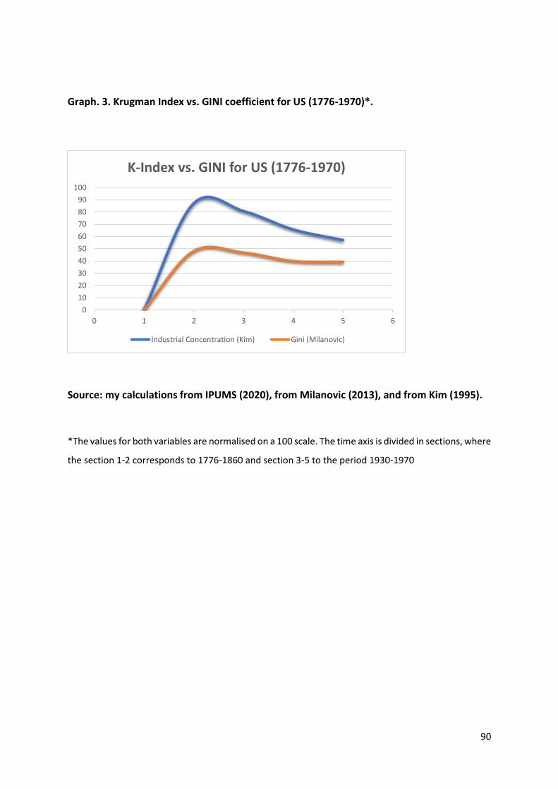
90
Graph. 3. Krugman Index vs. GINI coefficient for US (1776-1970)*.
Source: my calculations from IPUMS (2020), from Milanovic (2013), and from Kim (1995).
*The values for both variables are normalised on a 100 scale. The time axis is divided in sections, where
the section 1-2 corresponds to 1776-1860 and section 3-5 to the period 1930-1970
0
10
20
30
40
50
60
70
80
90
100
0 1 2 3 4 5 6
K-Index vs. GINI for US (1776-1970)
Industrial Concentration (Kim) Gini (Milanovic)
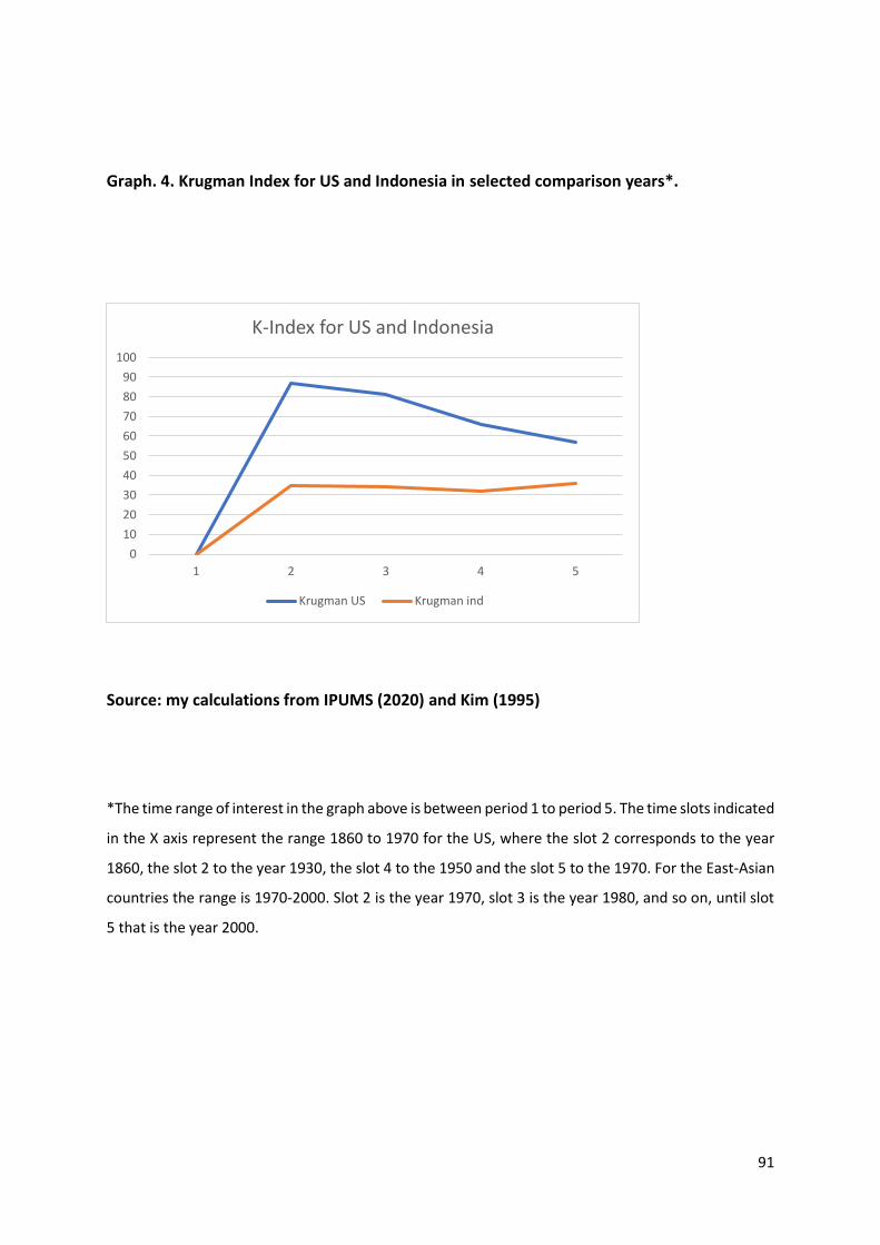
91
Graph. 4. Krugman Index for US and Indonesia in selected comparison years*.
Source: my calculations from IPUMS (2020) and Kim (1995)
*The time range of interest in the graph above is between period 1 to period 5. The time slots indicated
in the X axis represent the range 1860 to 1970 for the US, where the slot 2 corresponds to the year
1860, the slot 2 to the year 1930, the slot 4 to the 1950 and the slot 5 to the 1970. For the East-Asian
countries the range is 1970-2000. Slot 2 is the year 1970, slot 3 is the year 1980, and so on, until slot
5 that is the year 2000.
0
10
20
30
40
50
60
70
80
90
100
1 2 3 4 5
K-Index for US and Indonesia
Krugman US Krugman ind
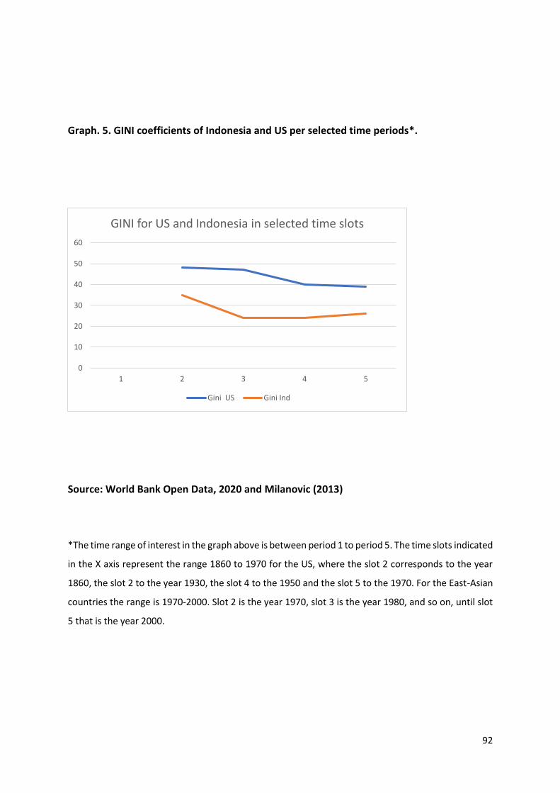
92
Graph. 5. GINI coefficients of Indonesia and US per selected time periods*.
Source: World Bank Open Data, 2020 and Milanovic (2013)
*The time range of interest in the graph above is between period 1 to period 5. The time slots indicated
in the X axis represent the range 1860 to 1970 for the US, where the slot 2 corresponds to the year
1860, the slot 2 to the year 1930, the slot 4 to the 1950 and the slot 5 to the 1970. For the East-Asian
countries the range is 1970-2000. Slot 2 is the year 1970, slot 3 is the year 1980, and so on, until slot
5 that is the year 2000.
0
10
20
30
40
50
60
1 2 3 4 5
GINI for US and Indonesia in selected time slots
Gini US Gini Ind
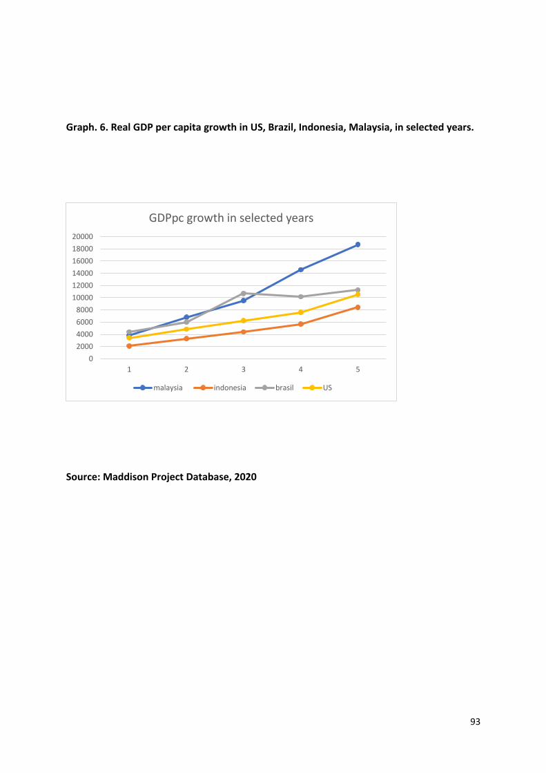
93
Graph. 6. Real GDP per capita growth in US, Brazil, Indonesia, Malaysia, in selected years.
Source: Maddison Project Database, 2020
0
2000
4000
6000
8000
10000
12000
14000
16000
18000
20000
1 2 3 4 5
GDPpc growth in selected years
malaysia indonesia brasil US
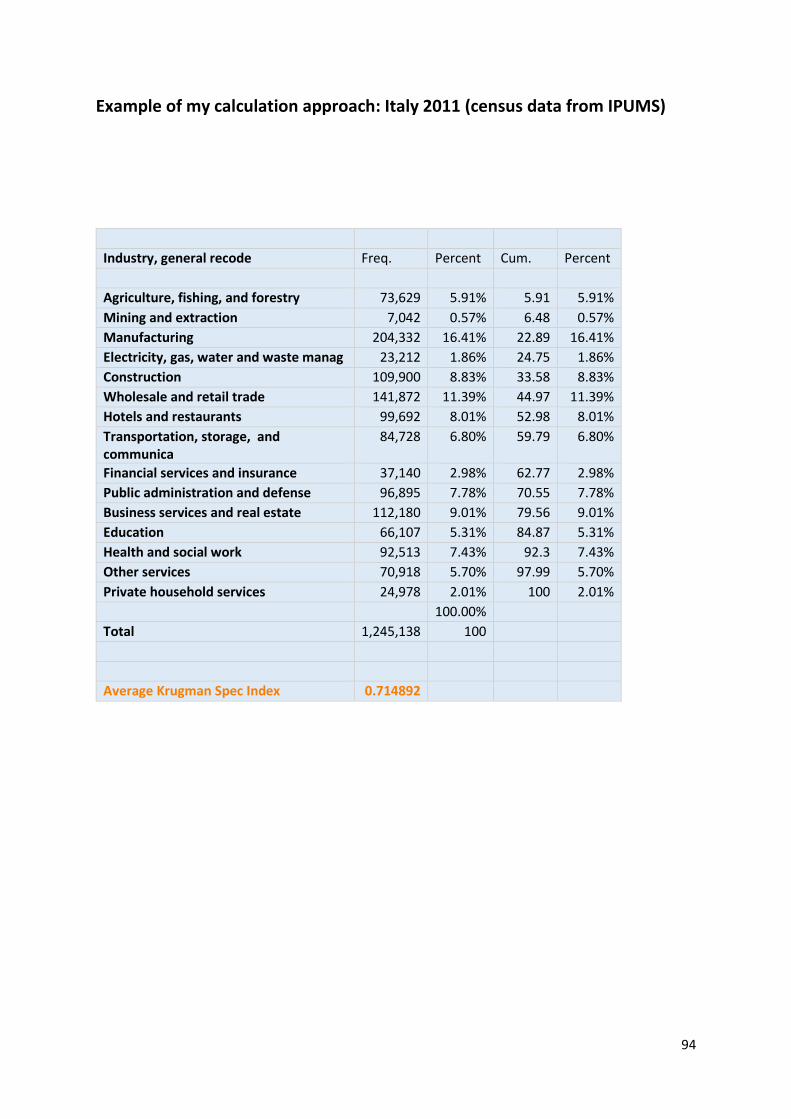
94
Example of my calculation approach: Italy 2011 (census data from IPUMS)
Industry, general recode Freq. Percent Cum. Percent
Agriculture, fishing, and forestry 73,629 5.91% 5.91 5.91%
Mining and extraction 7,042 0.57% 6.48 0.57%
Manufacturing 204,332 16.41% 22.89 16.41%
Electricity, gas, water and waste manag 23,212 1.86% 24.75 1.86%
Construction 109,900 8.83% 33.58 8.83%
Wholesale and retail trade 141,872 11.39% 44.97 11.39%
Hotels and restaurants 99,692 8.01% 52.98 8.01%
Transportation, storage, and communica
84,728 6.80% 59.79 6.80%
Financial services and insurance 37,140 2.98% 62.77 2.98%
Public administration and defense 96,895 7.78% 70.55 7.78%
Business services and real estate 112,180 9.01% 79.56 9.01%
Education 66,107 5.31% 84.87 5.31%
Health and social work 92,513 7.43% 92.3 7.43%
Other services 70,918 5.70% 97.99 5.70%
Private household services 24,978 2.01% 100 2.01% 100.00%
Total 1,245,138 100
Average Krugman Spec Index 0.714892
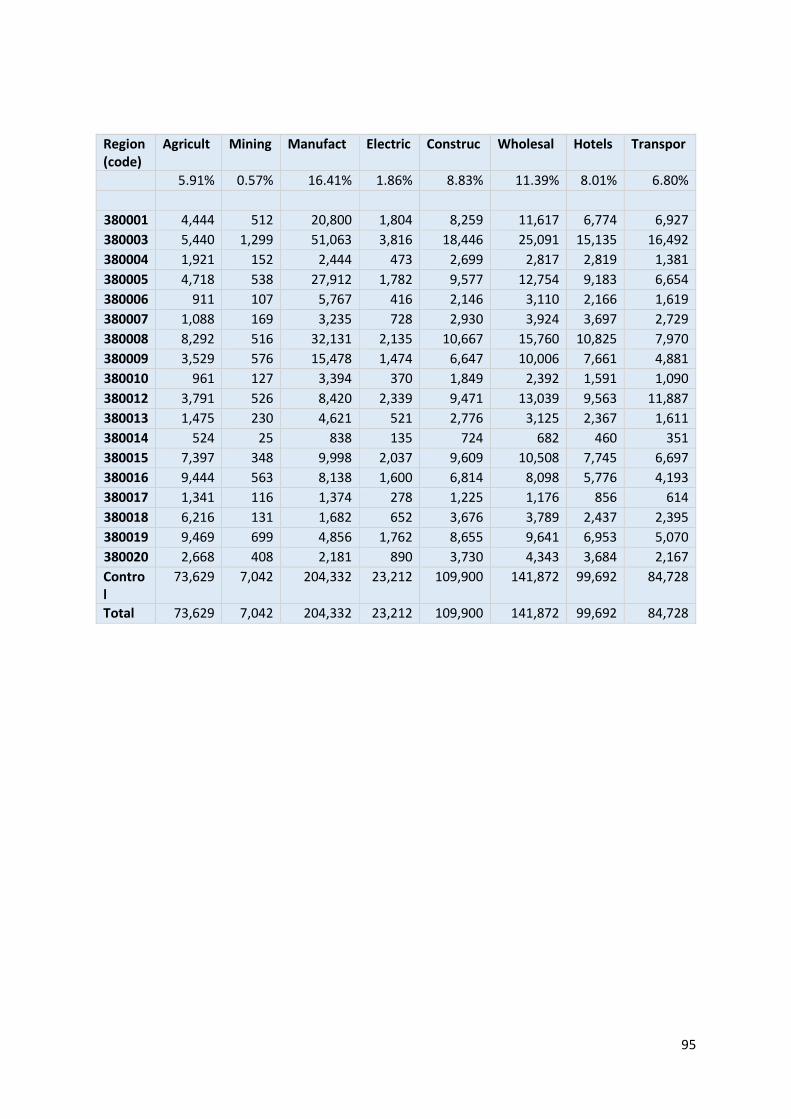
95
Region (code)
Agricult Mining Manufact Electric Construc Wholesal Hotels Transpor
5.91% 0.57% 16.41% 1.86% 8.83% 11.39% 8.01% 6.80%
380001 4,444 512 20,800 1,804 8,259 11,617 6,774 6,927
380003 5,440 1,299 51,063 3,816 18,446 25,091 15,135 16,492
380004 1,921 152 2,444 473 2,699 2,817 2,819 1,381
380005 4,718 538 27,912 1,782 9,577 12,754 9,183 6,654
380006 911 107 5,767 416 2,146 3,110 2,166 1,619
380007 1,088 169 3,235 728 2,930 3,924 3,697 2,729
380008 8,292 516 32,131 2,135 10,667 15,760 10,825 7,970
380009 3,529 576 15,478 1,474 6,647 10,006 7,661 4,881
380010 961 127 3,394 370 1,849 2,392 1,591 1,090
380012 3,791 526 8,420 2,339 9,471 13,039 9,563 11,887
380013 1,475 230 4,621 521 2,776 3,125 2,367 1,611
380014 524 25 838 135 724 682 460 351
380015 7,397 348 9,998 2,037 9,609 10,508 7,745 6,697
380016 9,444 563 8,138 1,600 6,814 8,098 5,776 4,193
380017 1,341 116 1,374 278 1,225 1,176 856 614
380018 6,216 131 1,682 652 3,676 3,789 2,437 2,395
380019 9,469 699 4,856 1,762 8,655 9,641 6,953 5,070
380020 2,668 408 2,181 890 3,730 4,343 3,684 2,167
Control
73,629 7,042 204,332 23,212 109,900 141,872 99,692 84,728
Total 73,629 7,042 204,332 23,212 109,900 141,872 99,692 84,728

96
Finance Public Busines Education Health Other ser Privat Total Control
2.98% 7.78% 9.01% 5.31% 7.43% 5.70% 2.01%
3,279 5,692 9,577 4,594 7,845 5,393 2,170 99,687 99,687
8,973 9,282 24,302 10,202 16,555 12,761 5,019 223,876 223,876
732 2,027 1,659 1,750 2,497 1,192 281 24,844 24,844
3,226 5,334 9,566 5,052 8,030 6,227 1,746 112,299 112,299
936 2,347 2,330 1,471 2,318 1,416 417 27,477 27,477
970 2,733 3,427 1,513 3,001 1,946 1,025 33,115 33,115
3,966 7,191 11,395 6,038 9,874 8,229 2,562 137,551 137,551
2,575 5,335 7,770 3,659 5,993 5,245 1,895 82,724 82,724
469 1,456 1,583 984 1,367 1,238 553 19,424 19,424
4,210 14,270 13,157 5,944 8,670 8,506 3,860 117,653 117,653
687 2,445 2,169 1,476 1,976 1,547 333 27,359 27,359
103 665 416 392 505 325 64 6,209 6,209
2,044 10,171 7,719 7,056 6,230 5,081 1,806 94,446 94,446
1,574 7,375 5,378 4,389 5,144 3,957 745 73,188 73,188
228 1,191 783 690 806 531 112 11,321 11,321
668 4,091 2,508 2,489 2,287 1,388 366 34,775 34,775
1,848 11,507 6,108 6,547 6,536 4,187 1,131 84,969 84,969
652 3,783 2,333 1,861 2,879 1,749 893 34,221 34,221
37,140 96,895 112,180 66,107 92,513 70,918 24,978
1,245,138
37,140 96,895 112,180 66,107 92,513 70,918 24,978
1,245,138
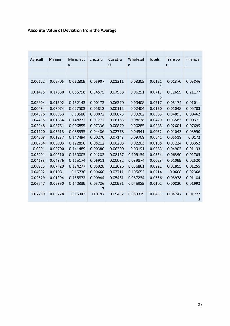
97
Absolute Value of Deviation from the Average
Agricult Mining Manufactu
Electrici Construct
Wholesale
Hotels Transport
Financial
0.00122 0.06705 0.062309 0.05907 0.01311 0.03205 0.01211
0.01370 0.05846
0.01475 0.17880 0.085798 0.14575 0.07958 0.06291 0.07175
0.12659 0.21177
0.03304 0.01592 0.152143 0.00173 0.06370 0.09408 0.0517 0.05174 0.01011
0.00494 0.07074 0.027503 0.05812 0.00112 0.02404 0.0120 0.01048 0.05703
0.04676 0.00953 0.13588 0.00072 0.06873 0.09202 0.0583 0.04893 0.00462
0.04435 0.01834 0.148272 0.01272 0.06163 0.08628 0.0429 0.03583 0.00371
0.05348 0.06761 0.006855 0.07336 0.00879 0.00285 0.0285 0.02601 0.07695
0.01120 0.07613 0.088355 0.04486 0.02778 0.04341 0.0032 0.01043 0.03950
0.04608 0.01237 0.147494 0.00270 0.07143 0.09708 0.0641 0.05518 0.0172
0.00764 0.06903 0.122896 0.08212 0.00208 0.02203 0.0158 0.07224 0.08352
0.0391 0.02700 0.141489 0.00380 0.06300 0.09191 0.0563 0.04903 0.01133
0.05201 0.00210 0.160003 0.01282 0.08167 0.109134 0.0754 0.06390 0.02705
0.04133 0.04376 0.115174 0.06911 0.00082 0.039874 0.0023 0.01099 0.02520
0.06913 0.07429 0.124277 0.05028 0.02626 0.056861 0.0221 0.01855 0.01255
0.04092 0.01081 0.15738 0.00666 0.07711 0.105652 0.0714 0.0608 0.02368
0.02529 0.01294 0.155872 0.00944 0.05481 0.087234 0.0556 0.03978 0.01184
0.06947 0.09360 0.140339 0.057267
0.00951 0.045985 0.0102 0.00820 0.01993
0.02289 0.05228 0.15343 0.0197 0.05432 0.083329 0.0431 0.04247 0.012273

98
Public Business services
Education Health Other ser
Private h KSIr
0.019075 0.004723 0.016401 0.010499 0.01909 0.066816 0.455718
0.017976 0.12654 0.101233 0.104648 0.122984 0.180876 1.631991
0.056899 0.075306 0.02662 0.047309 0.040148 0.008811 0.729386
0.022769 0.004821 0.023329 0.012499 0.03085 0.049841 0.41016
0.053597 0.069324 0.03084 0.049243 0.036989 0.003366 0.708919
0.049613 0.059545 0.030205 0.041861 0.029516 0.020976 0.685822
0.003604 0.011483 0.038245 0.032432 0.059079 0.08251 0.571796
0.022759 0.020831 0.002258 0.009519 0.017003 0.055806 0.473088
0.062792 0.075983 0.038207 0.059523 0.039499 0.002079 0.791748
0.069454 0.02719 0.036823 0.019417 0.062985 0.134476 0.827806
0.052585 0.070759 0.030765 0.05294 0.035142 0.006729 0.731922
0.070956 0.086386 0.047162 0.068841 0.052373 0.017498 0.927386
0.027151 0.021285 0.053644 0.006958 0.01469 0.052243 0.524631
0.001705 0.042154 0.0133 0.018696 0.001159 0.009766 0.54113
0.065527 0.083115 0.042654 0.065587 0.049468 0.015576 0.876447
0.035598 0.067738 0.015441 0.049579 0.037384 0.005408 0.663993
0.040939 0.035646 0.045944 0.00365 0.002084 0.025219 0.608119
0.038776 0.069297 0.024941 0.043179 0.032294 0.015691 0.707996 0.714892
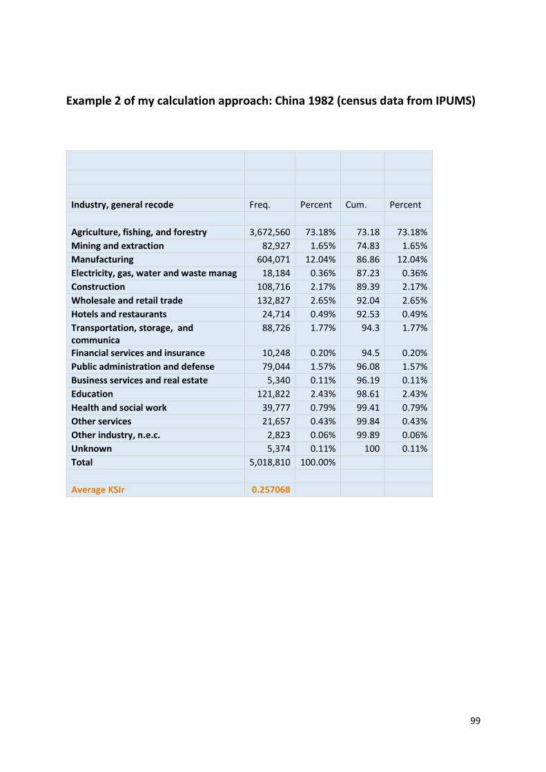
99
Example 2 of my calculation approach: China 1982 (census data from IPUMS)
Industry, general recode Freq. Percent Cum. Percent
Agriculture, fishing, and forestry 3,672,560 73.18% 73.18 73.18%
Mining and extraction 82,927 1.65% 74.83 1.65%
Manufacturing 604,071 12.04% 86.86 12.04%
Electricity, gas, water and waste manag 18,184 0.36% 87.23 0.36%
Construction 108,716 2.17% 89.39 2.17%
Wholesale and retail trade 132,827 2.65% 92.04 2.65%
Hotels and restaurants 24,714 0.49% 92.53 0.49%
Transportation, storage, and communica
88,726 1.77% 94.3 1.77%
Financial services and insurance 10,248 0.20% 94.5 0.20%
Public administration and defense 79,044 1.57% 96.08 1.57%
Business services and real estate 5,340 0.11% 96.19 0.11%
Education 121,822 2.43% 98.61 2.43%
Health and social work 39,777 0.79% 99.41 0.79%
Other services 21,657 0.43% 99.84 0.43%
Other industry, n.e.c. 2,823 0.06% 99.89 0.06%
Unknown 5,374 0.11% 100 0.11%
Total 5,018,810 100.00%
Average KSIr 0.257068
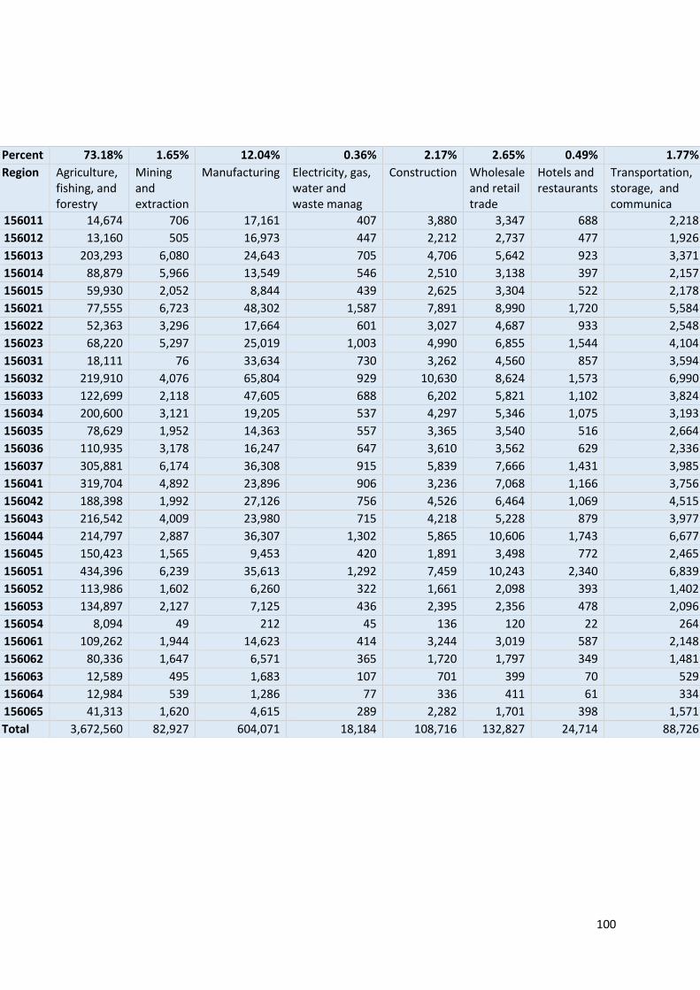
100
Percent 73.18% 1.65% 12.04% 0.36% 2.17% 2.65% 0.49% 1.77%
Region Agriculture, fishing, and forestry
Mining and extraction
Manufacturing Electricity, gas, water and waste manag
Construction Wholesale and retail trade
Hotels and restaurants
Transportation, storage, and communica
156011 14,674 706 17,161 407 3,880 3,347 688 2,218
156012 13,160 505 16,973 447 2,212 2,737 477 1,926
156013 203,293 6,080 24,643 705 4,706 5,642 923 3,371
156014 88,879 5,966 13,549 546 2,510 3,138 397 2,157
156015 59,930 2,052 8,844 439 2,625 3,304 522 2,178
156021 77,555 6,723 48,302 1,587 7,891 8,990 1,720 5,584
156022 52,363 3,296 17,664 601 3,027 4,687 933 2,548
156023 68,220 5,297 25,019 1,003 4,990 6,855 1,544 4,104
156031 18,111 76 33,634 730 3,262 4,560 857 3,594
156032 219,910 4,076 65,804 929 10,630 8,624 1,573 6,990
156033 122,699 2,118 47,605 688 6,202 5,821 1,102 3,824
156034 200,600 3,121 19,205 537 4,297 5,346 1,075 3,193
156035 78,629 1,952 14,363 557 3,365 3,540 516 2,664
156036 110,935 3,178 16,247 647 3,610 3,562 629 2,336
156037 305,881 6,174 36,308 915 5,839 7,666 1,431 3,985
156041 319,704 4,892 23,896 906 3,236 7,068 1,166 3,756
156042 188,398 1,992 27,126 756 4,526 6,464 1,069 4,515
156043 216,542 4,009 23,980 715 4,218 5,228 879 3,977
156044 214,797 2,887 36,307 1,302 5,865 10,606 1,743 6,677
156045 150,423 1,565 9,453 420 1,891 3,498 772 2,465
156051 434,396 6,239 35,613 1,292 7,459 10,243 2,340 6,839
156052 113,986 1,602 6,260 322 1,661 2,098 393 1,402
156053 134,897 2,127 7,125 436 2,395 2,356 478 2,096
156054 8,094 49 212 45 136 120 22 264
156061 109,262 1,944 14,623 414 3,244 3,019 587 2,148
156062 80,336 1,647 6,571 365 1,720 1,797 349 1,481
156063 12,589 495 1,683 107 701 399 70 529
156064 12,984 539 1,286 77 336 411 61 334
156065 41,313 1,620 4,615 289 2,282 1,701 398 1,571
Total 3,672,560 82,927 604,071 18,184 108,716 132,827 24,714 88,726

101
Financial services and insurance
Public administration and defense
Business services and real estate
Education Health and social work
0.001372 0.031442 0.00782 0.058868 0.008295
0.001031 0.012365 0.003302 0.021861 0.006259
7.83E-05 0.005252 0.000274 0.002678 0.000382
0.000579 0.005588 0.000318 0.004775 0.001302
0.001401 0.014326 0.000794 0.011275 0.003088
0.000436 0.006606 0.002231 0.008418 0.004552
0.001207 0.007189 0.001263 0.01371 0.004128
0.000864 0.016111 0.00188 0.014208 0.006464
0.000848 0.006272 0.003469 0.019264 0.009892
0.000443 0.004194 0.000258 0.002325 0.002289
0.000155 0.004192 0.000343 0.005428 3.72E-05
0.000495 0.00587 0.000573 0.004007 0.001538
0.000506 0.001755 0.000443 0.00201 0.000658
6.79E-05 0.00016 0.000236 0.00027 0.000727
0.000284 0.004385 0.000434 0.003125 0.000831
0.000529 0.0052 0.000538 0.001824 0.001
5.54E-05 0.001692 0.000142 0.001084 0.000168
0.000531 0.001106 0.000517 0.003262 0.001983
0.000499 0.002726 0.000308 0.002692 2.45E-05
0.000296 0.004502 0.000677 0.003888 0.002363
0.000481 0.00497 0.000501 0.006839 0.001392
5.01E-05 0.001036 0.000712 0.005621 0.002804
8.47E-05 0.002422 0.000648 0.006837 0.002151
0.000239 0.02219 0.000284 0.007895 0.001507
0.000185 0.000435 0.000264 0.006641 0.001556
3.03E-05 0.000972 0.00039 0.002032 0.000673
0.001016 0.011719 0.000938 0.003251 0.001694
0.000131 0.006833 7.96E-05 0.006995 0.00047
0.001443 0.010863 6.92E-05 0.00416 0.002256
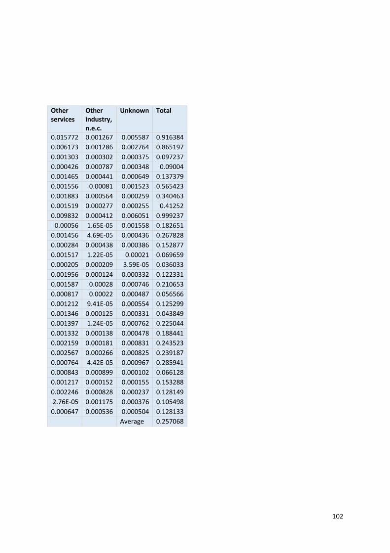
102
Other services
Other industry, n.e.c.
Unknown Total
0.015772 0.001267 0.005587 0.916384
0.006173 0.001286 0.002764 0.865197
0.001303 0.000302 0.000375 0.097237
0.000426 0.000787 0.000348 0.09004
0.001465 0.000441 0.000649 0.137379
0.001556 0.00081 0.001523 0.565423
0.001883 0.000564 0.000259 0.340463
0.001519 0.000277 0.000255 0.41252
0.009832 0.000412 0.006051 0.999237
0.00056 1.65E-05 0.001558 0.182651
0.001456 4.69E-05 0.000436 0.267828
0.000284 0.000438 0.000386 0.152877
0.001517 1.22E-05 0.00021 0.069659
0.000205 0.000209 3.59E-05 0.036033
0.001956 0.000124 0.000332 0.122331
0.001587 0.00028 0.000746 0.210653
0.000817 0.00022 0.000487 0.056566
0.001212 9.41E-05 0.000554 0.125299
0.001346 0.000125 0.000331 0.043849
0.001397 1.24E-05 0.000762 0.225044
0.001332 0.000138 0.000478 0.188441
0.002159 0.000181 0.000831 0.243523
0.002567 0.000266 0.000825 0.239187
0.000764 4.42E-05 0.000967 0.285941
0.000843 0.000899 0.000102 0.066128
0.001217 0.000152 0.000155 0.153288
0.002246 0.000828 0.000237 0.128149
2.76E-05 0.001175 0.000376 0.105498
0.000647 0.000536 0.000504 0.128133 Average 0.257068