inductive querying with virtual mining views

Inductive Querying with Virtual Mining

Views

Hendrik Blockeel, Toon Calders, Elisa Fromont, Bart Goethals, AdrianaPrado, and Celine Robardet

Abstract In an inductive database, one can not only query the data storedin the database, but also the patterns that are implicitly present in thesedata. In this chapter, we present an inductive database system in which thequery language is traditional SQL. More specifically, we present a system inwhich the user can query the collection of all possible patterns as if they werestored in traditional relational tables. We show how such tables, or miningviews, can be developed for three popular data mining tasks, namely itemsetmining, association rule discovery and decision tree learning. To illustrate theinteractive and iterative capabilities of our system, we describe a completedata mining scenario that consists in extracting knowledge from real geneexpression data, after a pre-processing phase.

Hendrik BlockeelKatholieke Universiteit Leuven, BelgiumLeiden Institute of Advanced Computer Science, Universiteit Leiden, The Nether-lands e-mail: [email protected]

Toon CaldersTechnische Universiteit Eindhoven, The Netherlands e-mail: [email protected]

Elisa Fromont · Adriana PradoUniversite de Lyon (Universite Jean Monnet), CNRS, Laboratoire Hubert Curien,UMR5516, F-42023 Saint-Etienne, France e-mail: {elisa.fromont,adriana.bechara.prado}@univ-st-etienne.fr

Bart GoethalsUniversiteit Antwerpen, Belgium e-mail: [email protected]

Celine RobardetUniversite de Lyon, INSA-Lyon, CNRS, LIRIS, UMR5205, F-69621, France e-mail:[email protected]

1

2 Authors Suppressed Due to Excessive Length

1 Introduction

Data mining is an interactive process in which different tasks may be per-formed sequentially. In addition, the output of those tasks may be repeatedlycombined to be used as input for subsequent tasks. For example, one could(a) first learn a decision tree model from a given dataset and, subsequently,mine association rules which describe the misclassified tuples with respect tothis model or (b) first look for an interesting association rule that describesa given dataset and then find all tuples that violate such rule.

In order to effectively support such a knowledge discovery process, theintegration of data mining into database systems has become necessary. Theconcept of Inductive Database Systems has been proposed in [1] so as toachieve such integration. The idea behind this type of system is to give tothe user the ability to query not only the data stored in the database, butalso patterns that can be extracted from these data. Such database shouldbe able to store and manage patterns as well as provide the user with theability to query them.

In this chapter, we show how such an inductive database system can beimplemented in practice, as studied in [2, 3, 4, 5, 6, 7]. To allow the users toquery patterns as well as standard data, several researchers proposed exten-sions to the popular query language SQL as a natural way to express suchmining queries [8, 9, 10, 11, 12, 13]. As opposed to those proposals, we presenthere an inductive database system in which the query language is traditionalSQL. We propose a relational database model based on what we call virtual

mining views. The mining views are relational tables that virtually containthe complete output of data mining tasks. For example, for the itemset min-ing task, there is a table called Sets virtually storing all itemsets. As far as theuser is concerned, all itemsets are stored in table Sets and can be queried asany other relational table. In reality, however, table Sets is empty. Whenevera query is formulated selecting itemsets from this table, the database systemtriggers an itemset mining algorithm, such as Apriori [14], which computesthe itemsets in the same way as normal views in databases are only computedat query time. The user does not notice the emptiness of the tables; he orshe can simply assume their existence and query accordingly. Therefore, weprefer to name these special tables virtual mining views.

In this chapter, we show how such tables, or virtual mining views, canbe developed for three popular data mining tasks, namely itemset mining,association rule discovery and decision tree learning. To make the model asgeneric as possible, the output of these tasks are represented by a unifyingset of mining views. In Section 2, we present these mining views in detail.

Since the proposed mining views are empty, they need to be filled (mate-rialized) by the system once a query is posed over them. The mining processitself needs to be performed by the system in order to answer such queries.Note that the user may impose certain constraints in his or her queries, ask-ing for only a subset of all possible patterns. As an example, the user may

Inductive Querying with Virtual Mining Views 3

query from the mining view Sets all frequent itemsets with a certain support.Therefore, the entire set of patterns does not always need to be stored in themining views, but only those that satisfy the constrains imposed by the user.In [2], Calders et al. present an algorithm that extracts from a query a setof constraints relevant for association rules to be pushed into the mining al-gorithm. We have extended this constraint extraction algorithm to extractconstraints from queries over decision trees. The reader can refer to [7] forthe details on the algorithm.

All ideas presented here, from querying the mining views and extractingconstraints from the queries to the actual execution of the data mining processitself and the materialization of the mining views, have been implementedinto the well-known open source database system PostgreSQL1. Details ofthe implementation are given in Section 3.

We have therefore organized the rest of this chapter in the following way.The next section is dedicated to the virtual mining views framework. Wealso present how the 4 prototypical tasks described in the previous chaptercan be executed by SQL queries over the mining views. The implementationof the system along with an extended illustrative data mining scenario ispresented in Section 3. Finally, the conclusions of this chapter are presentedin Section 4, stressing the main contributions and pointing to related futurework.

2 The Mining Views Framework

In this section, we present the mining views framework in detail. This frame-work consists of a set of relational tables, called mining views, which virtuallyrepresent the complete output of data mining tasks. In reality, the miningviews are empty and the database system finds the required tuples only whenthey are queried by the user.

2.1 The Mining View Concepts

We assume to be working in a relational database which contains the tableT (A1, . . . , An), having only categorical attributes. We denote the domain ofAi by dom(Ai), for all i = 1 . . . n. A tuple of T is therefore an elementof dom(Ai) × . . . × dom(An). The active domain of Ai of T , denoted byadom(Ai, T ), is defined as the set of values that are currently assigned to Ai,that is, adom(Ai, T ) := {t.Ai | t ∈ T }.

1 http://www.postgresl.org/


In the mining views framework, the patterns extracted from table T aregenerically represented by what we call concepts. We denote a concept asa conjunction of attribute-value pairs that is definable over table T . Forexample,

(Outlook = ‘Sunny’ ∧ Humidity = ‘High’ ∧ Play = ‘No’)

is a concept defined over the classical relational data table Playtennis [24], asample of which is illustrated in Figure 1.

PlaytennisDay Outlook Temperature Humidity Wind Play

D1 Sunny Hot High Weak NoD2 Sunny Hot High Strong NoD3 Overcast Hot High Weak YesD4 Rain Mild High Weak Yes. . . . . . . . . . . . . . . . . .

Fig. 1 The data table Playtennis.

To represent each concept as a database tuple, we use the symbol ‘?’ asthe wildcard value and assume it does not exist in the active domain of anyattribute of T .

Definition 1. A concept over table T is a tuple (c1, . . . , cn) with ci ∈adom(Ai) ∪ {‘?’}, for all i=1 . . . n.

Following Definition 1, the example concept above is represented by thetuple

(‘?’, ‘Sunny’, ‘?’, ‘?’, ‘High’, ‘?’, ‘No’).

We are now ready to introduce the mining view T Concepts . In the pro-posed framework, the mining view T Concepts(cid , A1, . . . , An) virtually con-tains all concepts that are definable over table T . We assume that theseconcepts can be sorted in lexicographic order and that an identifier can un-ambiguously be given to each concept.

Definition 2. The mining view T Concepts(cid , A1, . . . , An) contains onetuple (cid , c1, . . . , cn) for every concept defined over table T . The attributecid uniquely identifies the concepts.

In fact, the mining view T Concepts represents exactly a data cube [25]built from table T , with the difference that the wildcard value “ALL” intro-duced in [25] is replaced by the value ‘?’. By following the syntax introducedin [25], the mining view T Concepts would be created with the SQL queryshown in Figure 2 (consider adding the identifier cid after its creation).


1. create table T_Concepts2. select A1, A2,..., An3. from T4. group by cube A1, A2,..., An

Fig. 2 The data cube that represents the contents of the mining view T Concepts.

2.2 Representing Patterns and Models as Sets of

Concepts

We now explain how patterns extracted from the table Playtennis can berepresented by the concepts in the mining view Playtennis Concepts . In theremainder of this section, we refer to table Playtennis as T and use theconcepts in Figure 3 for the illustrative examples.

Playtennis Concepts

cid Day Outlook Temperature Humidity Wind Play

. . . . . . . . . . . . . . . . . . . . .

101 ? ? ? ? ? Yes102 ? ? ? ? ? No103 ? Sunny ? High ? ?104 ? Sunny ? High ? No105 ? Sunny ? Normal ? Yes106 ? Overcast ? ? ? Yes107 ? Rain ? ? Strong No108 ? Rain ? ? Weak Yes109 ? Rain ? High ? No110 ? Rain ? Normal ? Yes. . . . . . . . . . . . . . . . . . . . .

Fig. 3 A sample of the mining view Playtennis Concepts, which is used for theillustrative examples in Section 2.2.

2.2.1 Itemsets and Association Rules

As itemsets in a relational database are conjunctions of attribute-value pairs,they can be represented as concepts. Itemsets are represented in the proposedframework by the mining view:

T Sets(cid , supp, sz ).

The view T Sets contains a tuple for each itemset, where cid is the iden-tifier of the itemset (concept), supp is its support (the number of tuples


satisfied by the concept), and sz is its size (the number of attribute-valuepairs in which there are no wildcards).

Similarly, association rules are represented by the view:

T Rules(rid , cida, cidc, cid , conf ).

T Rules contains a tuple for each association rule that can be extractedfrom table T . We assume that a unique identifier, rid , can be given to eachrule. The attribute rid is the rule identifier, cida is the identifier of the conceptrepresenting its left hand side (referred to here as antecedent), cidc is theidentifier of the concept representing its right hand side (referred to here asconsequent), cid is the identifier of the union of the last two, and conf is theconfidence of the rule.

Figure 4 shows the mining views T Sets and T Rules, and illustrates howthe rule “if outlook is sunny and humidity is high, you should not play tennis”is represented in these views by using three of the concepts given in Figure 3.

T Sets

cid supp sz

102 5 1103 3 2104 3 3. . . . . . . . .

T Rules

rid cida cidc cid conf

1 103 102 104 100%. . . . . . . . . . . . . . .

Fig. 4 Mining views for representing itemsets and association rules. The attributescida, cidc, and cid refer to concepts given in Figure 3.

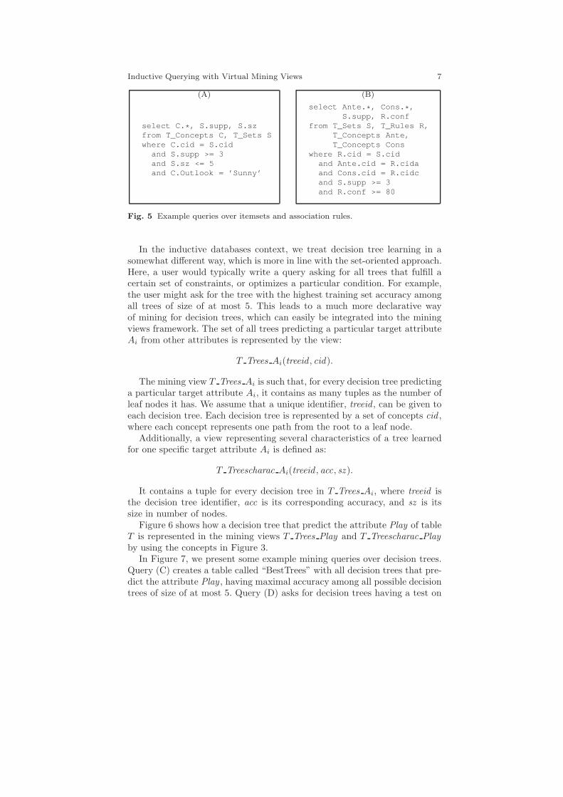
In Figure 5, queries (A) and (B) are example mining queries over itemsetsand association rules, respectively. Query (A) asks for itemsets having sup-port of at least 3 and size of at most 5, while query (B) asks for associationrules having support of at least 3 and confidence of at least 80%. Note thatthese two common data mining tasks and the well known constraints “mini-mum support” and “minimum confidence” can be expressed quite naturallywith SQL queries over the mining views.

2.2.2 Decision Trees

A decision tree learner typically learns a single decision tree from a dataset.This setting strongly contrasts with discovery of itemsets and associationrules, which is set-oriented: given certain constraints, the system finds allitemsets or association rules that fit the constraints. In decision tree learning,given a set of (sometimes implicit) constraints, one tries to find one tree thatfulfills the constraints and, besides that, optimizes some other criteria, whichare again not specified explicitly but are a consequence of the algorithm used.


(A) (B)

select C.*, S.supp, S.szfrom T_Concepts C, T_Sets Swhere C.cid = S.cid

and S.supp >= 3and S.sz <= 5and C.Outlook = ’Sunny’

select Ante.*, Cons.*,S.supp, R.conf

from T_Sets S, T_Rules R,T_Concepts Ante,T_Concepts Cons

where R.cid = S.cidand Ante.cid = R.cidaand Cons.cid = R.cidcand S.supp >= 3and R.conf >= 80

Fig. 5 Example queries over itemsets and association rules.

In the inductive databases context, we treat decision tree learning in asomewhat different way, which is more in line with the set-oriented approach.Here, a user would typically write a query asking for all trees that fulfill acertain set of constraints, or optimizes a particular condition. For example,the user might ask for the tree with the highest training set accuracy amongall trees of size of at most 5. This leads to a much more declarative wayof mining for decision trees, which can easily be integrated into the miningviews framework. The set of all trees predicting a particular target attributeAi from other attributes is represented by the view:

T Trees Ai(treeid , cid).

The mining view T Trees Ai is such that, for every decision tree predictinga particular target attribute Ai, it contains as many tuples as the number ofleaf nodes it has. We assume that a unique identifier, treeid , can be given toeach decision tree. Each decision tree is represented by a set of concepts cid ,where each concept represents one path from the root to a leaf node.

Additionally, a view representing several characteristics of a tree learnedfor one specific target attribute Ai is defined as:

T Treescharac Ai(treeid , acc, sz ).

It contains a tuple for every decision tree in T Trees Ai, where treeid isthe decision tree identifier, acc is its corresponding accuracy, and sz is itssize in number of nodes.

Figure 6 shows how a decision tree that predict the attribute Play of tableT is represented in the mining views T Trees Play and T Treescharac Play

by using the concepts in Figure 3.In Figure 7, we present some example mining queries over decision trees.

Query (C) creates a table called “BestTrees” with all decision trees that pre-dict the attribute Play , having maximal accuracy among all possible decisiontrees of size of at most 5. Query (D) asks for decision trees having a test on


Outlook

sunnyrrrrr

rrrrr

overcast rainII

III

IIII

Humidity

high��

�

��

normal::

:

::::

?>=<89:;Yes Windy

strong

weak66

6

6666

?>=<89:;No ?>=<89:;Yes ?>=<89:;No ?>=<89:;Yes

T Trees Play

treeid cid

1 1041 1051 1061 1071 108

. . . . . .

T Treescharac Play

treeid acc sz

1 100% 8. . . . . . . . .

Fig. 6 Mining views representing a decision tree which predicts the attribute Play .Each attribute cid of view T Trees Play refers to a concept given in Figure 3.

“Outlook=Sunny” and on “Wind=Weak”, with a size of at most 5 and anaccuracy of at least 80%.

(C) (D)

create table BestTrees asselect T.treeid, C.*, D.*from T_Concepts C,

T_Trees_Play T,T_Treescharac_Play D

where T.cid = C.cidand T.treeid = D.treeidand D.sz <= 5and D.acc =

(select max(acc)from T_Treescharac_Playwhere sz <= 5)

select T1.treeid,C1.*, C2.*

from T_Trees_Play T1,T_Trees_Play T2,T_Concepts C1,T_Concepts C2,T_Treescharac_Play D

where C1.Outlook = ‘Sunny’and C2.Wind = ‘Weak’and T1.cid = C1.cidand T2.cid = C2.cidand T1.treeid = T2.treeidand T1.treeid = D.treeidand D.sz <= 5and D.acc >= 80

Fig. 7 Example queries over decision trees.


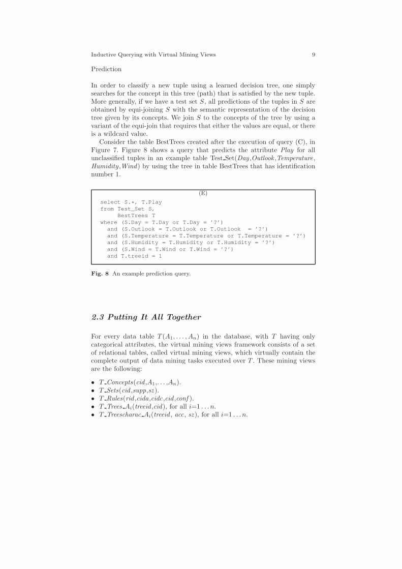
Prediction

In order to classify a new tuple using a learned decision tree, one simplysearches for the concept in this tree (path) that is satisfied by the new tuple.More generally, if we have a test set S, all predictions of the tuples in S areobtained by equi-joining S with the semantic representation of the decisiontree given by its concepts. We join S to the concepts of the tree by using avariant of the equi-join that requires that either the values are equal, or thereis a wildcard value.

Consider the table BestTrees created after the execution of query (C), inFigure 7. Figure 8 shows a query that predicts the attribute Play for allunclassified tuples in an example table Test Set(Day ,Outlook ,Temperature,Humidity ,Wind) by using the tree in table BestTrees that has identificationnumber 1.

(E)

select S.*, T.Playfrom Test_Set S,

BestTrees Twhere (S.Day = T.Day or T.Day = ’?’)

and (S.Outlook = T.Outlook or T.Outlook = ’?’)and (S.Temperature = T.Temperature or T.Temperature = ’?’)and (S.Humidity = T.Humidity or T.Humidity = ’?’)and (S.Wind = T.Wind or T.Wind = ’?’)and T.treeid = 1

Fig. 8 An example prediction query.

2.3 Putting It All Together

For every data table T (A1, . . . , An) in the database, with T having onlycategorical attributes, the virtual mining views framework consists of a setof relational tables, called virtual mining views, which virtually contain thecomplete output of data mining tasks executed over T . These mining viewsare the following:

• T Concepts(cid ,A1,. . . ,An).• T Sets(cid ,supp,sz ).• T Rules(rid ,cida,cidc,cid ,conf ).• T Trees Ai(treeid ,cid), for all i=1 . . . n.• T Treescharac Ai(treeid , acc, sz ), for all i=1 . . . n.


As shown in the examples given in this section, in order to retrieve patternsover table T , the user simply needs to write SQL queries over the proposedmining views. The semantics of these queries is the same as that of queriesover traditional relational tables. For more example queries over the miningviews, we refer the reader to [7].

Another important thing to note is that if the user wants to mine itemsets,association rules, or learn a decision tree from only a portion of table T , heor she should first create a new table T ′ from T , applying the appropriateselections and (or) projections. Then, the mining views associated with T ′,which are automatically created, will represent the patterns extracted fromthat corresponding portion of the data.

2.4 Mining Views vs. Data Mining Tasks

We now present how the 4 prototypical tasks described in the previous chap-ter can be executed by SQL queries over the mining views.

2.4.1 Discretization task: Discretize attribute Temperature into 3

intervals. The discretized attribute should be used in the

subsequent tasks

Since the data mining query language is SQL, our approach does not offerany new operator for pre-processing tasks. The discretization task can thusbe performed by creating a new table called “MyPlaytennis” with the SQLCASE query introduced in the previous chapter (when presenting the MINERULE operator).

2.4.2 Area task: Find all intra-tuple itemsets with relative

support of at least 20%, size of at least 2, and area, that is,

absolut support × size, of at least 10

The area task can be performed with an SQL query involving the miningviews MyPlaytennis Concepts and MyPlaytennis Sets , which are created au-tomatically after the creation of table MyPlaytennis for the discretizationtask. The query is shown below. Notice that the property area can be con-strained quite naturally in our framework (see line 6), due to the flexibilityof ad hoc querying.


1. select C.*, S.supp, S.sz,S.supp * S.sz as area

2. from MyPlaytennis_Sets S,MyPlaytennis_Concepts C

3. where C.cid = S.cid4. and S.supp >= 35. and S.sz >= 26. and S.supp * S.sz >= 10

2.4.3 Right hand side task: Find all intra-tuple association rules

with relative support of at least 20%, confidence of at most

80%, size of at most 3, and a singleton right hand size

Since the next task (lift task) requires a post-processing query over the resultsoutput by this one, it is necessary to store these results so that they can befurther queried. The SQL query to perform the right hand side task is thefollowing:

1. create table MyRules as2. select Ant.Day as DayA, ... ,Ant.Play as PlayA,

Con.Day as DayC, ..., Con.Play as PlayC,R.conf, SCon.supp/14 as suppC

3. from MyPlaytennis_Sets S, MyPlaytennis_Rules R,MyPlaytennis_Concepts Ant,MyPlaytennis_Concepts Con,MyPlaytennis_Sets SCon

4. where R.cid = S.cid5. and Ant.cid = R.cida6. and Con.cid = R.cidc7. and S.supp >= 38. and R.conf >= 809. and S.sz <= 310. and SCon.cid = R.cidc11. and SCon.sz = 1

The query above creates a new table called “MyRules”. We also store inthis table the confidence of the rules along with the relative supports of theirconsequents, since they are necessary to perform the lift task (the number 14,which is used to compute the relative supports of the consequents, refers tothe total number of tuples in table MyPlaytennis). Observe that the miningviews framework does not restrain the user from any format in which therules are to be stored, thanks again to the flexibility of ad hoc querying.


2.4.4 Lift task: Find, from the result of the right hand side task,

rules with attribute Play as consequent that have a lift

greater than 1

In order to perform the lift task, one needs to query table MyRules, createdfor the previous task. The query in question is the one depicted below:

1. select M.*, (M.conf/100)/M.suppC as lift2. from MyRules M3. where M.PlayC <> ’?’4. and (M.conf/100)/M.suppC >=1

Note that the two constraints required by the lift task can be expressedquite naturally in our framework. In line 3, we assure that the rules in theresult have the attribute Play as consequent, i.e., it is not a wildcard value.In line 4, we compute the property lift of the rules.

2.5 Conclusions

Observe that the mining views framework is able to perform all data miningtasks described in the previous chapter without any type of pre- or post-processing, as opposed to the other proposals. Also note that the choice of theschema for representing itemsets and association rules implicitly determinesthe complexity of the queries a user needs to write. For instance, by addingthe attributes sz and supp to the mining views T Sets, the area constraintcan be expressed quite naturally in our framework. Without these attributes,one could still obtain their values. Nevertheless, it would imply that the userwould have to write more complicated queries.

The addition of the attribute cid in the mining view T Rules can be jus-tified by the same argument. Indeed, one of the 3 concept identifiers for anassociation rule, cid , cida or cidc is redundant, as it can be determined fromthe other two. However, this redundancy eases query writing. Still with re-gard to the mining view T Rules, while the query for association rule miningseems to be more complex than the queries for the same purpose in otherdata mining query languages (e.g., in MSQL), one could easily turn it intoa view definition so that association rules can be mined with simple queriesover that database view.

It is also important to notice that some types of tasks are not easily ex-pressed with the mining views. For example, if the tuples over which the datamining tasks are to be executed come from different tables in the database,a new table containing these tuples should be created before the mining canstart. In DMQL, MINE RULE, SPQL the relevant set of tuples can be spec-ified in the query itself. In the case of DMX, this can be done while training


the model. Another example is the extraction of inter-tuple patterns, whichare possible to be performed with DMQL, MINE RULE, SPQL, and DMX.To mine inter-tuple patterns in the mining views framework, one would needto first pre-process the dataset that is to be mined, by changing its repre-sentation: the relevant attributes of a group of tuples should be added toa single tuple of a new table. Constraints on the corresponding groups oftuples being considered, which are allowed to be specified in the proposalsmentioned above, can be specified in a post-processing step over the results.Our proposal is more related to MSQL and SIQL, as they also only allow theextraction of intra-tuple patterns over a single relation.

Some data mining tasks that can be performed in SIQL and DMX, such asclustering, cannot currently be executed with the proposed mining views. Onthe other hand, note that one could always extend the framework by definingnew mining views that represent clusterings, as studied in [7]. In fact, onedifference between our approach and those presented in the previous chapteris the fact that to extend the formalism, it is necessary to define new miningviews or simply add new attributes to the existing ones, whereas in otherformalisms one would need to extend the language itself.

To finalize, although the mining views do not give the user the ability toexpress every type of query the user can think of (similarly to any relationaldatabase), the set of mining tasks that can be executed by the system isconsistent and large enough to cover several steps in a knowledge discoveryprocess.

We now list how the mining views overcome the drawbacks found in atleast one of the proposals surveyed in the previous chapter:

2.5.1 Satisfaction of the closure principle

Since, in the proposed framework, the data mining query language is standardSQL, the closure principle is clearly satisfied.

2.5.2 Flexibility to specify different kinds of patterns

The mining views framework provides a very clear separation between thepatterns it currently represents, which in turn can be queried in a very declar-ative way (SQL queries). In addition to itemsets, association rules and deci-sion trees, the flexibility of ad hoc querying allows the user to think of newtypes of patterns which may be derived from those currently available. Forexample, in [7] we show how frequent closed itemsets [26] can be extractedfrom a given table T with an SQL query over the available mining viewsT Concepts and T Sets .


2.5.3 Flexibility to specify ad hoc constraints

The mining views framework is meant to offer exactly this flexibility: byvirtue of a full-fledged query language that allows of ad hoc querying, theuser can think of new constraints that were not considered at the time ofimplementation. An example is the constraint lift, which could be computedby the framework for the execution of the lift task.

2.5.4 Intuitive way of representing mining results

In the mining views framework, patterns are all represented as sets of con-cepts, which makes the framework as generic as possible, not to mention thatthe patterns are easily interpretable.

2.5.5 Support for post-processing of mining results

Again, thanks to the flexibility of ad hoc querying, post-processing of miningresults is clearly feasible in the mining views framework.

3 An Illustrative Scenario

One of the main advantages of our system is the flexibility of ad hoc querying,that is, the user can iteratively specify new types of constraints and querythe patterns in combination with the data themselves. In this section, weillustrate this feature with a complete data mining scenario that consists inextracting knowledge from real gene expression data, after an extensive pre-processing phase. Differently to the scenario presented in [6], here we do notlearn a classifier, but mine for non-redundant correct association rules.

We begin by presenting how the implementation of our inductive databasesystem was realized. Next, the aforementioned scenario is presented.

3.1 Implementation

Our inductive database system was developed into the well-known opensource database system PostgreSQL2, which is written in C language. Everytime a data table is created into our system, its mining views are automati-

2 http://www.postgresl.org/


cally created. Accordingly, if this data table is removed from the system, itsmining views are deleted as well.

Fig. 9 The proposed inductive database system implemented into PostgreSQL.

The main steps of the system are illustrated in Figure 9. When the userwrites a query, PostgreSQL generates a data structure representing its corre-sponding relational algebra expression. A call to our Mining Extension wasadded to PostgreSQL’s source code after the generation of this data struc-ture. In the Mining Extension, which was implemented in C language, weprocess the relational algebra structure. If it refers to one or more miningviews, we then extract the constraints (as described in detail in [7]), triggerthe data mining algorithms and materialize the virtual mining views withthe obtained mining results. Just after the materialization (i.e., upon returnfrom the miningExtension() call), the work-flow of the database system con-tinues and the query is executed as if the patterns or models were there allthe time. We refer the reader to [5, 7] for more details on the implementationand efficiency evaluation of the system.

Additionally, we adapted the web-based administration tool PhpPgAd-min3 so as to have a user-friendly interface to the system.

3.2 Scenario

The scenario presented in this section consists in extracting knowledge fromthe gene expression data which resulted from a biological experimentationconcerning the transcription of Plasmodium Falciparum [27] during its repro-duction cycle (IDC) within the human blood cells.

The Plasmodium Falciparum is a parasite that causes human malaria. Thedata gather the expression profiles of 472 genes of this parasite in 46 different

3 http://phppgadmin.sourceforge.net/


biological samples.4 Each gene is known to belong to a specific biologicalfunction. Each sample in turn corresponds to a time point (hour) of the IDC,which lasts for 48 hours. During this period, the merozoite (initial stage ofthe parasite) evolves to 3 different identified stages: Ring, Trophozoite, andSchizont. In addition, due to reproduction, one merozoite leads to up to 32new ones during each cycle, after which a new developmental cycle is started.Figure 10 shows the percentage of parasites (y-axis) that are at the Ring(black curve), Trophozoite (light gray curve), or Schizont (dark gray curve)stage, at every time point of the IDC (x-axis).

Fig. 10 Major developmental stages of Plasmodium Falciparum parasite (Figurefrom [27]). The three curves, in different levels of gray, represent the percentage ofparasites (y-axis) that are at the Ring (black), Trophozoite (light gray), or Schizontstage (dark gray), at every time point of the IDC (x-axis).

These data were stored into 3 different tables in our system, as illustratedin Figure 11. They are the following:

• GeneFunctions(function id, function): represents the biological functions.There are in total 12 different functional groups.

• Samples(sample name, stage): represents the samples themselves. Twodata points are missing, namely the 23rd and 29th hours. We added tothis table the attribute called stage, the values of which are based on thecurves illustrated in Figure 10: this new attribute discriminates the sam-ples having at least 75% of the parasites in the Ring (stage=1), Trophozoite(stage=2) or Schizont (stage=3) stage. Samples that contain less than 75%of any parasite stage were assigned to stage 4, a “non-identified” stage.Thus, for our scenario, stage 1 corresponds to time points between 1 and16 hours; stage 2 corresponds to time points between 18 and 28 hours; andstage 3 gathers time points between 32 and 43 hours.

• Plasmodium(gene id, function id, tp 1, tp 2,. . . , tp 48): represents, foreach of the genes, its corresponding function and its expression profile.As proposed in [27], we take the logarithm to the base 2 of the raw ex-pression values.

4 The data is available at http://malaria.ucsf.edu/SupplementalData.php


Plasmodiumgene id function id tp 1 tp 2 . . . tp 48

1 12 -0.13 0.12 . . . 0.112 12 0.24 0.48 . . . -0.03

. . . . . . . . . . . . . . . . . .

472 5 1.2 0.86 ... 1.15

GeneFunctionsfunction id function

1 Actin myosin mobility2 Cytoplasmic translation machinery

. . . . . .

12 Transcription machinery

Samplessample name stage

tp 1 1tp 2 1. . . . . .

tp 48 4

Fig. 11 The Plasmodium data.

Having presented the data, we are now ready to describe the goal of ourscenario. In gene expression analysis, a gene is said to be highly expressed,according to a biological sample, if there are many RNA transcripts in theconsidered sample. These RNA transcripts can be translated into proteins,which can, in turn, influence the expression of other genes. In other words,it can make other genes also highly expressed. This process is called gene

regulation [27].In this context, analogously to what the biologists have studied in [27], we

want to characterize the parasite’s different stages by identifying the genesthat are active during each stage. More precisely, we want to identify, for eachdifferent stage, the functional groups whose genes have an unusual high levelof expression or, as the biologists say, are overexpressed in the correspondingset of samples. By considering the samples corresponding to a specific stageand the genes that are overexpressed within those samples, we might haveinsights into the regulation processes that occur during the development ofthe parasite. As pointed out in [27], understanding these regulation processeswould provide the foundation for future drug and vaccine development effortstoward eradication of the malaria.

Observe that decision trees are not appropriate for the analysis we wantto perform; they are most suited for predicting, which is not our intentionhere. Therefore, in our scenario we mine for association rules. A couple ofpre-processing steps have to be performed initially, such as the discretizationof the expression values. These steps are described in detail in the first 3 sub-sequent subsections. The remaining subsections show how the desired rulescan be extracted from the data.

3.2.1 Step 1: Pre-processing 1

Since our intention is to characterize the parasite’s stages by means of thefunctional groups and not of the individual genes themselves, we first create


a view on the data that groups the genes by the function they belong to. Thecorresponding pre-process query is shown below:5

1. create view PlasmodiumAvg as2. select G.function,3. avg(p.tp_1) as tp_1,4. ...,5. avg(p.tp_48) as tp_486. from Plasmodium P, GeneFunctions G7. where P.function_id = G.function_id8. group by G.function

The view called “PlasmodiumAvg” calculates, for every different func-tional group, the average expression profile (arithmetic mean) over all timepoints (see lines from 2 to 5).


Since we want the functional groups as components of the desired rules (an-tecedents and/or consequents), it is therefore necessary to transpose the viewPlasmodiumAvg, which was created in the previous step. In other words, weneed a new view in which the gene functional groups are the columns andthe expression profiles are the rows. To this end, we use the PostgreSQLfunction called crosstab6. As crosstab requires the data to be listed down thepage (not across the page), we first create a view on PlasmodiumAvg, called“PlasmodiumAvgTemp”, which lists data in such format. The correspondingqueries are shown below.

1. create view PlasmodiumAvgTemp as2. select function as tid, ‘tp_1’ as item,

tp_1 as val3. from PlasmodiumAvg4. union5. ...6. union7. select function as tid, ‘tp_48’ as item,

tp_48 as val8. from PlasmodiumAvg

5 For the sake of readability, ellipsis were added to some of the SQL queries presentedin this section and in the following ones, which represent sequences of attribute names,attribute values, clauses etc.6 We refer the reader to http://www.postgresql.org/docs/current/static/tablefunc.html for more details on the crosstab function.


9. create view PlasmodiumTranspose as10. select * from crosstab11. (‘select item, tid, val from PlasmodiumAvgTemp

order by item’,‘select distinct tid from PlasmodiumAvgTemp

order by item’)12. as (sample_name text, Actin_myosin_mobility real,

...,Transcription_machinery real)


Having created the transposed view PlasmodiumTranspose, the third andlast pre-processing step is to discretize the gene expression values so as toencode the expression property of each functional group of genes.

In gene expression data analysis, a gene is considered to be overexpressed ifits expression value is high with respect to its expression profile. One approachto identify the level of expression of a gene is the method called x% cut-off,which was proven to be successful in [28]: a gene is considered overexpressedif its expression value is among the x% highest values of its expression profile,and underexpressed otherwise. With x=50, a gene is tagged as overexpressedif its expression value is above the median value of its profile.

As in this scenario the data are log transformed (very high expressionvalues are deemphasized), the distribution of the data is symmetrical and,therefore, median expression values are very similar to mean values. As com-puting the mean value is straightforward in SQL and as we are not dealingwith genes independently, but with groups of genes, we use a slight adapta-tion of the 50% cut-off method: we encode the overexpression property bycomparing it to the mean value observed for each group, rather than themedian. We first create a view, called “PlasmodiumTransposeAvg”, whichcalculates, for every group of genes, its mean expression value. This compu-tation is performed by the following query:

1. create view PlasmodiumTransposeAvg as2. select avg(Actin_myosin_mobility) as avg_Actin_mm,3. ...4. avg(Transcription_machinery) as avg_Tran_m5. from PlasmodiumTranspose

Afterwards, we create the new table named “PlasmodiumSamples” ap-plying the aforementioned discretization rule. The query that performs thisdiscretization step is shown below. Notice that the attribute stage is alsoadded to the new table PlasmodiumSamples (see line 2).


1. create table PlasmodiumSamples as2. select P.sample_name, S.stage,3. case when P.Actin_myosin_mobility > avg_Actin_mm4. then ‘overexpressed’5. else6. ‘underexpressed’7. end as Actin_myosin_mobility,8. ...9. case when P.Transcription_machinery > avg_Tran_m10. then ‘overexpressed’11. else12. ‘underexpressed’13. end as Transcription_machinery14. from PlasmodiumTranspose P,

PlasmodiumTransposeAvg,Samples S

15. where P.sample_name = S.sample_name16. order by S.stage

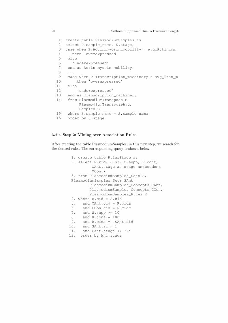
3.2.4 Step 2: Mining over Association Rules

After creating the table PlasmodiumSamples, in this new step, we search forthe desired rules. The corresponding query is shown below:

1. create table RulesStage as2. select R.rid, S.sz, S.supp, R.conf,

CAnt.stage as stage_antecedentCCon.*

3. from PlasmodiumSamples_Sets S,PlasmodiumSamples_Sets SAnt,

PlasmodiumSamples_Concepts CAnt,PlasmodiumSamples_Concepts CCon,PlasmodiumSamples_Rules R

4. where R.cid = S.cid5. and CAnt.cid = R.cida6. and CCon.cid = R.cidc7. and S.supp >= 108. and R.conf = 1009. and R.cida = SAnt.cid

10. and SAnt.sz = 111. and CAnt.stage <> ‘?’12. order by Ant.stage


As we want to characterize the parasite’s stages themselves by means ofthe gene functions, we look for rules having only the attribute stage as theantecedent (see lines 9, 10 and 11) and gene function(s) in the consequent. Ad-ditionally, since we want to characterize the stages without any uncertainty,we only look for correct association rules, that is, rules with a confidenceof 100% (see line 8). Finally, as the shortest stage is composed of 10 timepoints in total (not considering the dummy stage), we set 10 as the minimumsupport (line 7). The 381 resultant rules are eventually stored in the tablecalled “RulesStage” (see line 1).

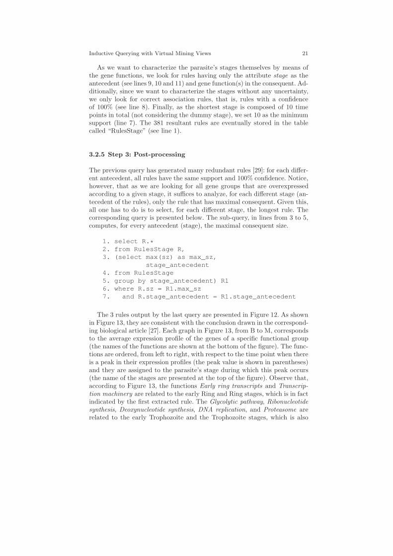
3.2.5 Step 3: Post-processing

The previous query has generated many redundant rules [29]: for each differ-ent antecedent, all rules have the same support and 100% confidence. Notice,however, that as we are looking for all gene groups that are overexpressedaccording to a given stage, it suffices to analyze, for each different stage (an-tecedent of the rules), only the rule that has maximal consequent. Given this,all one has to do is to select, for each different stage, the longest rule. Thecorresponding query is presented below. The sub-query, in lines from 3 to 5,computes, for every antecedent (stage), the maximal consequent size.

1. select R.*2. from RulesStage R,3. (select max(sz) as max_sz,

stage_antecedent4. from RulesStage5. group by stage_antecedent) R16. where R.sz = R1.max_sz7. and R.stage_antecedent = R1.stage_antecedent

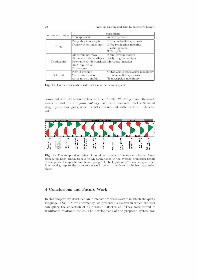
The 3 rules output by the last query are presented in Figure 12. As shownin Figure 13, they are consistent with the conclusion drawn in the correspond-ing biological article [27]. Each graph in Figure 13, from B to M, correspondsto the average expression profile of the genes of a specific functional group(the names of the functions are shown at the bottom of the figure). The func-tions are ordered, from left to right, with respect to the time point when thereis a peak in their expression profiles (the peak value is shown in parentheses)and they are assigned to the parasite’s stage during which this peak occurs(the name of the stages are presented at the top of the figure). Observe that,according to Figure 13, the functions Early ring transcripts and Transcrip-

tion machinery are related to the early Ring and Ring stages, which is in factindicated by the first extracted rule. The Glycolytic pathway, Ribonucleotide

synthesis, Deoxynucleotide synthesis, DNA replication, and Proteasome arerelated to the early Trophozoite and the Trophozoite stages, which is also


antecedent (stage)consequent

overexpressed underexpressed

Ring

Early ring transcripts Deoxynucleotide synthesisTranscription machinery DNA replication machine

Plastid genomeTCA cycle

Trophozoite

Glycolytic pathway Actin myosin motorsRibonucleotide synthesis Early ring transcriptsDeoxynucleotide synthesis Merozoite invasionDNA replicationProteasome

SchizontPlastid genome Cytoplasmic translation machineryMerozoite invasion Ribonucleotide synthesisActin myosin mobility Transcription machinery

Fig. 12 Correct association rules with maximum consequent.

consistent with the second extracted rule. Finally, Plastid genome, MerozoiteInvasion, and Actin myosin mobility have been associated to the Schizontstage by the biologists, which is indeed consistent with the third extractedrule.

Fig. 13 The temporal ordering of functional groups of genes (an adapted figurefrom [27]). Each graph, from B to M, corresponds to the average expression profileof the genes of a specific functional group. The biologists of [27] have assigned eachfunctional group to the parasite’s stage in which it achieves its highest expressionvalue.

4 Conclusions and Future Work

In this chapter, we described an inductive database system in which the querylanguage is SQL. More specifically, we presented a system in which the usercan query the collection of all possible patterns as if they were stored intraditional relational tables. The development of the proposed system was


motivated by the need to (a) provide an intuitive framework that coversdifferent kinds of patterns in a generic way and, at the same time, allows of(b) ad hoc querying, (c) definition of meaningful operations and (d) queryingof mining results.

As for future work, we identify the following three directions:

• Currently, the mining views are in fact empty and only materialized uponrequest. Therefore, inspired by the work of Harinarayan et al. [30], thefirst direction for further research is to investigate which mining views(or which parts of them) could actually be materialized in advance. Thiswould speed up query evaluation.

• Our system deals with intra-tuple patterns only. To mine inter-tuple pat-terns, one would need to first pre-process the dataset that is to be mined,by changing its representation. Although this is not a fundamental prob-lem, this pre-processing step may be laborious. For example, in the contextof market basket analysis, a table would need to be created in which eachtransaction is represented as a tuple with as many boolean attributes asare the possible items that can be bought by a customer. An interest-ing direction for future work would then be to investigate how inter-tuplepatterns can be integrated into the system.

• Finally, the prototype developed so far covers only itemset mining, associ-ation rules and decision trees. An obvious direction for further work is toextend it with other models, taking into account the exhaustiveness natureof the queries the users are allowed to write.

Acknowledgements This work has been partially supported by the projects IQ(IST-FET FP6-516169) 2005/8, GOA 2003/8 “Inductive Knowledge bases”, FWO“Foundations for inductive databases”, and BINGO2 (ANR-07-MDCO 014-02). Whenthis research was performed, Hendrik Blockeel was a post-doctoral fellow of the Re-search Foundation - Flanders (FWO-Vlaanderen), Elisa Fromont was working at theKatholieke Universteit Leuven, and Adriana Prado was working at the University ofAntwerp.

References

1. Imielinski, T., Mannila, H.: A database perspective on knowledge discovery.Communications of the ACM 39 (1996) 58–64

2. Calders, T., Goethals, B., Prado, A.: Integrating pattern mining in relationaldatabases. In: Proc. ECML-PKDD. (2006) 454–461

3. Fromont, E., Blockeel, H., Struyf, J.: Integrating decision tree learning into in-ductive databases. In: ECML-PKDD Workshop KDID (Revised selected papers).(2007) 81–96

4. Blockeel, H., Calders, T., Fromont, E., Goethals, B., Prado, A.: Mining views:Database views for data mining. In: ECML-PKDD Workshop CMILE. (2007)

5. Blockeel, H., Calders, T., Fromont, E., Goethals, B., Prado, A.: Mining views:Database views for data mining. In: Proc. IEEE ICDE. (2008)


6. Blockeel, H., Calders, T., Fromont, E., Goethals, B., Prado, A.: An inductivedatabase prototype based on virtual mining views. In: Proc. ACM SIGKDD.(2008)

7. Prado, A.: An Inductive Database System Based on Virtual Mining Views. PhDthesis, University of Antwerp, Belgium (December 2009)

8. Han, J., Fu, Y., Wang, W., Koperski, K., Zaiane, O.: DMQL: A data miningquery language for relational databases. In: ACM SIGMOD Workshop DMKD.(1996)

9. Imielinski, T., Virmani, A.: Msql: A query language for database mining. DataMining Knowledge Discovery 3(4) (1999) 373–408

10. Meo, R., Psaila, G., Ceri, S.: An extension to sql for mining association rules.Data Mining and Knowledge Discovery 2(2) (1998) 195–224

11. Wicker, J., Richter, L., Kessler, K., Kramer, S.: Sinbad and siql: An inductivedatabse and query language in the relational model. In: Proc. ECML-PKDD.(2008) 690–694

12. Bonchi, F., Giannotti, F., Lucchese, C., Orlando, S., Perego, R., Trasarti, R.: Aconstraint-based querying system for exploratory pattern discovery informationsystems. Information System (2008) Accepted for publication.

13. Tang, Z.H., MacLennan, J.: Data Mining with SQL Server 2005. John Wiley &Sons (2005)

14. Agrawal, R., Srikant, R.: Fast algorithms for mining association rules. In: Proc.VLDB. (1994) 487–499

15. Botta, M., Boulicaut, J.F., Masson, C., Meo, R.: Query languages supportingdescriptive rule mining: A comparative study. In: Database Support for DataMining Applications. (2004) 24–51

16. Han, J., Kamber, M.: Data Mining - Concepts and Techniques, 1st ed. MorganKaufmann (2000)

17. Han, J., Chiang, J.Y., Chee, S., Chen, J., Chen, Q., Cheng, S., Gong, W., Kam-ber, M., Koperski, K., Liu, G., Lu, Y., Stefanovic, N., Winstone, L., Xia, B.B.,Zaiane, O.R., Zhang, S., Zhu, H.: Dbminer: a system for data mining in relationaldatabases and data warehouses. In: Proc. CASCON. (1997) 8–12

18. Srikant, R., Agrawal, R.: Mining generalized association rules. Future GenerationComputer Systems 13(2–3) (1997) 161–180

19. Meo, R., Psaila, G., Ceri, S.: A tightly-coupled architecture for data mining. In:Proc. IEEE ICDE. (1998) 316–323

20. Mannila, H., Toivonen, H.: Levelwise search and borders of theories in knowledgediscovery. Data Mining and Knowledge Discovery 1(3) (1997) 241–258

21. Ng, R., Lakshmanan, L.V.S., Han, J., Pang, A.: Exploratory mining and pruningoptimizations of constrained associations rules. In: Proc. ACM SIGMOD. (1998)13–24

22. Pei, J., Han, J., Lakshmanan, L.V.S.: Mining frequent itemsets with convertibleconstraints. In: Proc. IEEE ICDE. (2001) 433–442

23. Bistarelli, S., Bonchi, F.: Interestingness is not a dichotomy: Introducing softnessin constrained pattern mining. In: Proc. PKDD. (2005) 22–33

24. Mitchell, T.M.: Machine Learning. McGraw-Hill, New York (1997)25. Gray, J., Chaudhuri, S., Bosworth, A., Layman, A., Reichart, D., Venkatrao, M.:

Data cube: A relational aggregation operator generalizing group-by, cross-tab,and sub-total. Data Mining and Knowledge Discovery (1996) 152–159

26. Pasquier, N., Bastide, Y., Taouil, R., Lakhal, L.: Discovering frequent closeditemsets for association rules. In: Proc. ICDT. (1999) 398–416

27. Bozdech, Z., Llinas, M., Pulliam, B.L., Wong, E.D., Zhu, J., DeRisi, J.L.: Thetranscriptome of the intraerythrocytic developmental cycle of plasmodium falci-parum. PLoS Biology 1(1) (2003) 1–16


28. Becquet, C., Blachon, S., Jeudy, B., Boulicaut, J.F., Gandrillon, O.: Strongassociation rule mining for large-scale gene-expression data analysis: a case studyon human SAGE data. Genome Biology 12 (2002)

29. Zaki, M.J.: Generating non-redundant association rules. In: Proc. ACMSIGKDD. (2000) 34–43

30. Harinarayan, V., Rajaraman, A., Ullman, J.D.: Implementing data cubes effi-ciently. In: Proc. ACM SIGMOD. (1996) 205–216

inductive querying with virtual mining views

Documents