induction machine speed estimation - lth induction machine models it is crucial to start with a good...
TRANSCRIPT

Induction MachineSpeed EstimationObservations on Observers
Bo Peterson

Department of
Industrial Electrical Engineering andAutomation (IEA)Lund Institute of Technology (LTH)Box 118S-221 00 LUNDSweden
http://www.iea.lth.se/
Copyright © 1996 Bo Peterson

Abstract
This work focuses on observers estimating flux linkage and speed forinduction machines, mainly in the low speed region. With speedestimation, sensorless control is possible, meaning that the speed ofinduction machines without mechanical speed sensors can be controlled.The observer based sensorless drive system has superior dynamicperformance compared to a system with an open loop frequency inverter,yet it is neither more complex nor expensive. Using mechanical equivalentmodels of the induction machine and observers, an accurate flux observerworking in the entire speed region of the induction machine is presented.The flux observer is expanded into a combined flux and speed observer,measuring only stator current and voltage. A method for sensorless controlis proposed, analyzed and experimentally verified. Observer and controllercalculations are performed by a digital signal processor.

Contents
Abstract 3
Contents 4
Acknowledgements 6
1 Introduction 7
Overview of the Thesis ......................................................................... 8
2 Induction Machine Models 9
Dynamic Model of the Induction Machine........................................... 9A First Approach to a Mechanical Model of the Induction Machine . 12
3 An Introduction to Flux Estimation 15
Estimator A - the Voltage Model ....................................................... 15Estimator B - the Current Model ........................................................ 18Estimator C - Open Loop Simulation ................................................. 20Estimator D - Identity Observer ......................................................... 21Mechanical Models of Estimators ...................................................... 27Mechanical Model A .......................................................................... 28Mechanical Model B........................................................................... 29Mechanical Model C........................................................................... 29Mechanical Model D .......................................................................... 30
4 Flux Observer Models 36
Settling Time ...................................................................................... 39Poles in Different Reference Frames .................................................. 42Parameter Sensitivity .......................................................................... 44Parameter Sensitivity Comparison Between Two Observers ............. 45Observer Gain Influence on Parameter Sensitivity............................. 58Flux Observer Conclusions................................................................. 58
5 Speed Observer Models 59
Introduction to Speed Estimation ....................................................... 60Velocity Observer, Approach 1 .......................................................... 62Velocity Observer, Approach 2 .......................................................... 63
5
Speed Calculation through Differentiation ......................................... 64Speed Observer Based on Integration................................................. 66Steady State Value of Speed Estimate................................................ 68Speed Observer Poles ......................................................................... 76Poles of Linearized Speed Observer ................................................... 78Sensitivity to Rotor Resistance ........................................................... 80Important Problems at Low Frequencies ............................................ 80Speed Observer Conclusions .............................................................. 83
6 Controller Structure 84
Controller Overview ........................................................................... 84Flux Controller ................................................................................... 87Torque Controller ............................................................................... 88Speed Controller ................................................................................. 89
7 Implementation 91
General Configuration of Laboratory Set-up...................................... 91Voltage Source Inverter Implementation ........................................... 95Observer Implementation ................................................................... 96Controller Implementation ................................................................. 97DSP programming .............................................................................. 98
8 Measurements 99
Step Change of Load Torque.............................................................. 99Step Change of Speed Reference...................................................... 103Slow Ramp of Speed Reference ....................................................... 106
9 Conclusion 109
Future Topics .................................................................................... 109
References 111
Appendix 115
A List of Symbols ......................................................................... 115B Mechanical Analogy ................................................................. 118C Mechanical Model of the Induction Machine........................... 120D Parameters of Machines............................................................ 123E Observer Poles .......................................................................... 124F Steady State Value of Speed Observer ..................................... 128G Non-linear Systems and Linearized Systems ........................... 131

Acknowledgements
I would like to thank my supervisors Jari Valis and Gustaf Olsson forintroducing me to the problems associated with control of electrical drivesand for guiding me through the rocky roads of research. I would also like tothank everybody at the Department of Industrial Electrical Engineering andAutomation for helping me with all kinds of practical problems.

1Introduction
The induction motor is the most widely used electrical motor in industrialapplications. The majority of induction machines are used in constantspeed drives, but during the last decades the introduction of newsemiconductor devices has made variable speed drives with inductionmachines available.
Variable speed induction motors are usually fed by open loop frequencyinverters. The rotor speed of the machine is not measured, and a change inload torque will result in a change in speed. The dynamic performance isweak and problems such as oscillations are common.
The work presented in this thesis is a continuation of a work that startedwith studies of the oscillatory behaviour of inverter fed induction machines(Peterson, 1991). Methods were presented for damping of the oscillations.However, there is more to improve in open loop drives; fast acceleration,fast braking, fast reversal and constant speed independent of load changesare all desirable properties of a drive system. This requires a fast-actingand accurate torque control in the low speed region.
All those properties are obtained with vector controlled induction machines(Leonhard, 1985). The drawback of this method is that the rotor speed ofthe induction machine must be measured, which requires a speed sensor ofsome kind, for example a resolver or an incremental encoder. The cost ofthe speed sensor, at least for machines with ratings less than 10 kW, is inthe same range as the cost of the motor itself. The mounting of the sensorto the motor is also an obstacle in many applications. A sensorless systemwhere the speed is estimated instead of measured would essentially reducethe cost and complexity of the drive system. One of the main reasons thatinverter fed induction motor drives have become popular is that anystandard induction motor can be used without modifications. Note that theterm sensorless refers to the absence of a speed sensor on the motor shaft,and that motor currents and voltages must still be measured. The vectorcontrol method requires also estimation of the flux linkage of the machine,whether the speed is estimated or not.

8 Introduction
Research on sensorless control has been ongoing for more than 10 years(Haemmerli, 1986 and Tamai et al, 1987), and it is remarkable that reliablesensorless induction motor drive systems are not readily available. The aimof the work presented here is to derive an applicable method for sensorlesscontrol of induction machines. The system must work with standardinduction machines and the inverter hardware should not be considerablymore complex than present-day open loop frequency inverters.
Problems associated with sensorless control systems have mainly includedparameter sensitivity, integrator drift, and problems at low frequencies.Some have tried to solve these problems by redesigning the inductionmachine (Jansen et al, 1994a).
As it is most unfavourable using anything but standard machines, re-designed motors are not considered the best solution. The questions raisedin this work are: what is the best possible solution using standard motors?To what extent can the problems at low frequencies, and the parametersensitivity problems be reduced?
The feasibility of such a solution is highly facilitated by the arrival ofinexpensive digital signal processors. Even though basically the samehardware can be used for a sensorless system and a standard open loopdrive, the sensorless system requires substantially more computationcapacity.
Overview of the Thesis
After a general discussion on the induction machine model, an introductionto flux estimation is given, with the assumption that rotor current is zero. Adiscussion on flux estimation, now considering the fact that the rotorcurrent may differ from zero follows, assuming that the rotor speed can bemeasured. In the next chapter, methods for speed and flux estimation aredescribed when the measured speed signal is no longer available. Acombined speed and flux observer overcoming accuracy problems andintegrator drift problems at low frequencies in earlier attempts is presented.This is followed by a description of an experimental set-up used for testingthe proposed sensorless drive system. Finally the results obtained byexperiments are presented. Throughout the thesis, mechanical equivalentmodels are used to clarify the behaviour of the induction machine and theflux and speed estimators.

2Induction Machine Models
It is crucial to start with a good and appropriate model of the inductionmachine when designing flux observers. In this chapter a complete modelfor the induction machine as well as simplified models assuming that therotor current is zero will be discussed. The simplified models will later beused as a start when analyzing flux observers.
Dynamic Model of the Induction Machine
The standard vector equations (2.1)-(2.2) relating stator and rotor currentsand flux linkages (Kovács, 1984), including stator and rotor leakageinductances L sl and L rl , are written
ÁÁsT = Lsl + Lm( )is
T + LmirT (2.1)
ÁÁrT = L m is
T + L rl + L m( )irT (2.2)
and sometimes called the T-model, indicated by the T-superscript. This setof equations has one redundant parameter and can be rearranged into a setof equations with only one leakage inductance, LL (Slemon et al, 1980 andPeterson, 1991). The corresponding equations for this Γ -model with onlyone leakage inductance are
ÁÁs = L M is + ir( ) (2.3)
ÁÁr = ÁÁs + L Lir (2.4)
The vector differential equations for the stator flux ÁÁs, and the rotor flux
ÁÁr , here in the stator reference frame, and the torque equation are thesame for both models,
dÁÁs
dt= us − Rsis (2.5)
dÁÁr
dt= jzpωÁÁr − R rir (2.6)
Jdωdt
= T − Tload (2.7)

10 Induction Machine Models
where ω is the mechanical angular velocity of the rotor (rotor speed forshort). The scaling of the vectors is chosen so that the magnitude of thestator voltage vector is equal to the peak value of the phase-to-neutralvoltage, and the magnitude of the current vector is equal to the peak valueof the line current (Kovács, 1984). With this scaling, the driving torque Tof the motor can be expressed
T = 3
2zpℑ ÁÁs
∗is( ) = 3
2zpℑ ir
∗ÁÁs( ) = 3
2zpℑ ir
∗ÁÁr( ) (2.8)
where zp is the number of pole pairs. Throughout this thesis, voltage,current and flux vectors are represented as complex numbers. The complexconjugate of a vector v = vx + jvy is denoted v* = vx − jvy , and ℑ denotesimaginary part. The expression ℑ v∗w( ) = v x w y − v y w x of the complexvariables v and w is equivalent to the magnitude of the cross product of thevectors v and w.
A block diagram of the Γ-model, equations (2.3)-(2.7), is shown in Fig.2.1, where the upper part of the diagram is the real part of the vectorequations, and the lower part is the imaginary part of the equations.
Ψsx
1/LM
isxRs
+– ∫
– +
1/LL
+– Rr –
– ∫
zp
usx
ω
Ψrx
∫1/Jzp3
2 +–
+–
Tload
Ψsy1/LM
isyRs
–+ ∫
– +
1/LL
–+
Rr+– ∫
usy
Ψry
irx
iry
Fig. 2.1 Block diagram of the Γ-model.
Induction Machine Models 11
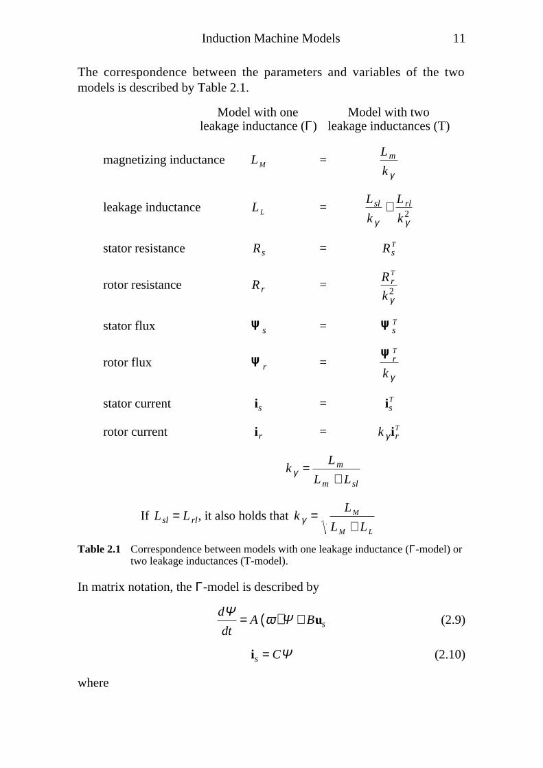
The correspondence between the parameters and variables of the twomodels is described by Table 2.1.
Model with one Model with twoleakage inductance (Γ) leakage inductances (T)
magnetizing inductance L M =Lm
k γ
leakage inductance L L =Lsl
k γ+ L rl
k γ2
stator resistance Rs = RsT
rotor resistance R r =R r
T
k γ2
stator flux ÁÁs = ÁÁsT
rotor flux ÁÁr =
ÁÁrT
k γ
stator current is = isT
rotor current ir = k γ irT
k γ = Lm
Lm + Lsl
If Lsl = L rl, it also holds that k γ = L M
L M + L L
Table 2.1 Correspondence between models with one leakage inductance (Γ-model) ortwo leakage inductances (T-model).
In matrix notation, the Γ-model is described by
dΨdt
= A ω( )Ψ + Bus (2.9)
is = CΨ (2.10)
where

12 Induction Machine Models
A (ω ) =
−Rs1
L M
+ 1
L L
Rs
L L
R r
L L
−R r
L L
+ jzpω
(2.11)
B =1
0
(2.12)
C = 1
L M
+ 1
L L
−1
L L
(2.13)
Ψ =
ÁÁs
ÁÁr
=Ψsx + jΨsy
Ψrx + jΨry
(2.14)
Note that the system described by equation (2.9) is a non-linear system, asthe rotor speed ω is varying. Saturation leads to variations in theinductances, and the resistances will vary with temperature, introducingadditional non-linearities.
A First Approach to a Mechanical Model of the InductionMachine
Matrices and equations give limited insight into the behaviour of a dynamicsystem. A mechanical equivalent model of the induction machine can beused to get a better understanding (Török et al, 1985 and Peterson, 1991).
A simplified example where the rotor current is assumed to be zero is usedas an introduction to the mechanical model. With this assumption,equations (2.3) and (2.5) give
dÁÁs
dt= us − Rsis = us − Rs
L M
ÁÁs (2.15)
With zero rotor current, there is no cross coupling between the x-axis andthe y-axis of equation (2.15). A block diagram of the x-axis (real axis)equation,
dΨsx
dt= usx − Rsisx = usx − Rs
L M
Ψsx (2.16)
is shown in Fig. 2.2, which basically is the shaded area of Fig. 2.1.
Induction Machine Models 13
+–
1/LM
Rs
usx Ψsx
isx
∫
Fig. 2.2 Block diagram of the x-axis equation
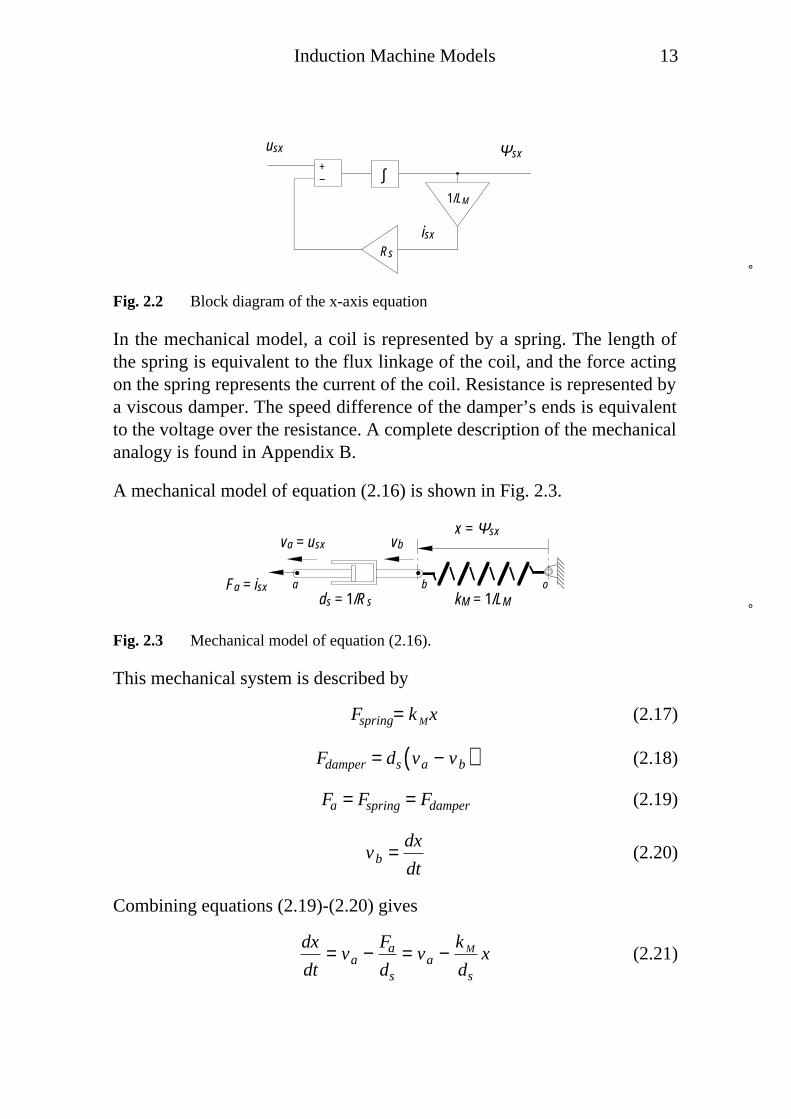
In the mechanical model, a coil is represented by a spring. The length ofthe spring is equivalent to the flux linkage of the coil, and the force actingon the spring represents the current of the coil. Resistance is represented bya viscous damper. The speed difference of the damper’s ends is equivalentto the voltage over the resistance. A complete description of the mechanicalanalogy is found in Appendix B.
A mechanical model of equation (2.16) is shown in Fig. 2.3.
va = usx
Fa = isx
x = Ψsx
kM = 1/LMds = 1/Rsa b
vb
o
Fig. 2.3 Mechanical model of equation (2.16).
This mechanical system is described by
Fspring= k Mx (2.17)
Fdamper = ds va − vb( ) (2.18)
Fa = Fspring = Fdamper (2.19)
vb = dx
dt(2.20)
Combining equations (2.19)-(2.20) gives
dx
dt= va − Fa
ds
= va − k M
ds
x (2.21)

14 Induction Machine Models
With the substitutions shown in Fig. 2.3, equation (2.21) is equal toequation (2.16). The mechanical model will be used later to clarify someproperties of a flux observer.
A complete mechanical model of the induction machine, including rotorcurrent and rotor flux, is found in Appendix C.

3An Introduction to Flux Estimation
In order to have a fast acting and accurate control of the induction machine,the flux linkage of the machine must be known. It is, however, expensiveand difficult to measure the flux. Instead, the flux can be estimated basedon measurements of voltage, current and angular velocity. There aredifferent control strategies for the induction machine. Some prefer statorflux control, while others prefer rotor flux control (Leonhard, 1985,Takahashi, 1989 and Lorenz, 1994). The estimators discussed in thischapter are mainly stator flux estimators, since stator flux control is used inlater chapters. Throughout this chapter, it is assumed that the rotor currentis zero, meaning that the induction machine is running at no load. InChapter 4, a more accurate estimator will be analyzed.
Estimator A - the Voltage Model
A first simple flux estimator is obtained from equation (2.5) in integralform,
ÁÁs = us − Rseis( )∫ dt (3.1)
often referred to as the voltage model. The ^ superscript denotes estimatedvalues, and index e denotes estimator parameter. Again, we consider onlythe real part of the equation, and assume the rotor current to be zero (noload torque). Most of the results obtained are valid for the imaginary axisas well, and also when load torque is present.
The estimator for the real axis
Ψsx = usx − Rseisx( )∫ dt (3.2)
is shown as a block diagram in Fig. 3.1.
The input to the estimator is the measured current and voltage of themachine. If the stator resistance Rse of the estimator is identical to theresistance Rs of the machine, and if the measured current and voltage arewithout any errors such as noise and offset errors, the output of thisestimator would be a perfect estimate of the stator flux, even if the rotor

16 An Introduction to Flux Estimation
current differs from zero. This is seen in equation (3.1), where the rotorcurrent does not appear.
+–
1/LM
Rs
usx
Ψsx
isx
+–
Ψsx
Rse
ˆ
machine estimator
∫ ∫
Fig. 3.1 Block diagram of estimator A.
Even the slightest error in Rse would cause the estimator to drift at lowfrequencies. Fig. 3.2 shows the drift of the estimate if the estimatorresistance parameter differs from the true resistance with 5 percent. Theinput voltage usx is a step from zero at t = 0 , and then held constant.
0
0.5
1
1.5
2
2.5
0 0.1 0.2 0.3 0.4 0.5 0.6 0.7 0.8 0.9 1
time [s]
psis
x (s
olid
) an
d ps
isxh
at (
dash
ed)
[Vs]
Rshat=0.95*RsRse = 0.95 Rs
t [s]
ˆΨ
sx (
solid
)
Ψsx
(da
shed
) [
Vs]
f = 0 Hz
Fig. 3.2 Simulation of estimator A, starting from zero. Rse = 0.95 Rs, f = 0 Hz (usx isconstant).
The machine parameters used throughout this thesis are for the IMEPinduction machine in ∆-connection, described in Appendix D. This 0.75kW machine is not representative to all induction machines. The p.u. stator
An Introduction to Flux Estimation 17
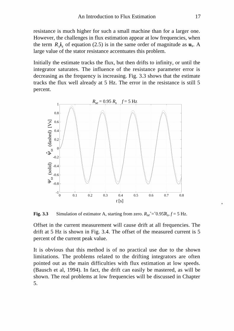
resistance is much higher for such a small machine than for a larger one.However, the challenges in flux estimation appear at low frequencies, whenthe term Rsis of equation (2.5) is in the same order of magnitude as us. Alarge value of the stator resistance accentuates this problem.
Initially the estimate tracks the flux, but then drifts to infinity, or until theintegrator saturates. The influence of the resistance parameter error isdecreasing as the frequency is increasing. Fig. 3.3 shows that the estimatetracks the flux well already at 5 Hz. The error in the resistance is still 5percent.
-1
-0.8
-0.6
-0.4
-0.2
0
0.2
0.4
0.6
0.8
1
0 0.1 0.2 0.3 0.4 0.5 0.6 0.7 0.8
time [s]
psis
x (s
olid
) an
d ps
isxh
at (
dash
ed)
[Vs]
Rshat=0.95*Rs, f=5 HzRse = 0.95 Rs
t [s]
ˆΨ
sx (
solid
)
Ψsx
(da
shed
) [
Vs]
f = 5 Hz
Fig. 3.3 Simulation of estimator A, starting from zero. Rse = 0.95 Rs, f = 5 Hz.
Offset in the current measurement will cause drift at all frequencies. Thedrift at 5 Hz is shown in Fig. 3.4. The offset of the measured current is 5percent of the current peak value.
It is obvious that this method is of no practical use due to the shownlimitations. The problems related to the drifting integrators are oftenpointed out as the main difficulties with flux estimation at low speeds.(Bausch et al, 1994). In fact, the drift can easily be mastered, as will beshown. The real problems at low frequencies will be discussed in Chapter5.

18 An Introduction to Flux Estimation
-1
-0.5
0
0.5
1
1.5
0 0.1 0.2 0.3 0.4 0.5 0.6 0.7 0.8
time [s]
psis
x (s
olid
) an
d ps
isxh
at (
dash
ed)
[Vs]
Rshat=0.95*Rs, f=5 Hz, offset in current: 5% of peak value
offset in measured current: 5% of peak current
Rse = 0.95 Rs
t [s]
ˆΨ
sx (
solid
)
Ψsx
(da
shed
) [
Vs]
f = 5 Hz
Fig. 3.4 Simulation of estimator A, starting from zero. Rse = 0.95 Rs, f = 5 Hz, 5%offset in measured current.
Estimator B - the Current Model
One way to eliminate the drift is to use equation (2.3) as a base for theestimator. Assuming zero rotor current, the estimated flux can becalculated,
Ψsx = Lmeisx (3.3)
shown in Fig. 3.5. Only the measured stator current is used as input to theestimator.
+–
1/LM
Rs
usxΨsx
isx ΨsxLMe
ˆ
machine estimator
∫
Fig. 3.5 Block diagram of estimator B.
An Introduction to Flux Estimation 19
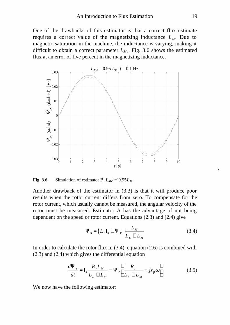
One of the drawbacks of this estimator is that a correct flux estimaterequires a correct value of the magnetizing inductance L M . Due tomagnetic saturation in the machine, the inductance is varying, making itdifficult to obtain a correct parameter LMe. Fig. 3.6 shows the estimatedflux at an error of five percent in the magnetizing inductance.
-0.03
-0.02
-0.01
0
0.01
0.02
0.03
0 1 2 3 4 5 6 7 8 9 10
time [s]
psis
x (s
olid
) an
d ps
isxh
at (
dash
ed)
[Vs]
LMhat=0.95*LM, f=0.1 HzLMe = 0.95 LM
t [s]
ˆΨ
sx (
solid
)
Ψsx
(da
shed
) [
Vs]
f = 0.1 Hz
Fig. 3.6 Simulation of estimator B, LMe = 0.95 LM.
Another drawback of the estimator in (3.3) is that it will produce poorresults when the rotor current differs from zero. To compensate for therotor current, which usually cannot be measured, the angular velocity of therotor must be measured. Estimator A has the advantage of not beingdependent on the speed or rotor current. Equations (2.3) and (2.4) give
ÁÁs = L Lis + ÁÁr( ) L M
L L + L M
(3.4)
In order to calculate the rotor flux in (3.4), equation (2.6) is combined with(2.3) and (2.4) which gives the differential equation
dÁÁr
dt= is
R rL M
L L + L M
− ÁÁrR r
L L + L M
− jzpω
(3.5)
We now have the following estimator:

20 An Introduction to Flux Estimation
ÁÁs = L Leis + ÁÁr( ) L Me
L Le + L Me
(3.6)
dÁÁr
dt= is
R reL Me
L Le + L Me
− ÁÁrR re
L Le + L Me
− jzpω
(3.7)
The resulting estimator requires measured rotor speed as well as measuredstator current as input, as indicated in the simplified block diagram in Fig.3.7. The estimator, referred to as the current model has good properties atlow frequencies but is sensitive to parameter errors at high frequencies(Jansen et al, 1994a).
ˆis
ω ˆflux
estimator
ÁÁÁÁs
ÁÁÁÁr
Fig. 3.7 Block diagram showing inputs and outputs of the current model.
Estimator C - Open Loop Simulation
To solve the drift problem of estimator A, the stator current can beestimated instead of measured. If ir = 0 , equations (2.3) and (2.5) suggestthe following observer,
Ψsx = usx − Rseisx( )∫ dt (3.8)
isx = Ψsx
L Me
(3.9)
shown in Fig. 3.8.
+–
1/LM
Rs
usx
Ψsx
isx
+–
Ψsx
Rse
ˆ
machine estimator
1/LMe
isxˆ
∫ ∫
Fig. 3.8 Block diagram of estimator C.

An Introduction to Flux Estimation 21
This estimator is basically an open loop simulation model of the machinesince it does not feed back any measurements.
Fig. 3.9 shows that the drift in Fig. 3.2 is no longer present. However, thereis a steady state error in the estimated flux due to the error in the resistance.
0
0.2
0.4
0.6
0.8
1
1.2
0 0.1 0.2 0.3 0.4 0.5 0.6 0.7 0.8 0.9 1
time [s]
psis
x (s
olid
) an
d ps
isxh
at (
dash
ed)
[Vs]
Rshat=0.95*RsRse = 0.95 Rs
t [s]
ˆΨ
sx (
solid
)
Ψsx
(da
shed
) [
Vs]
f = 0 Hz
Fig. 3.9 Simulation of estimator C, starting from zero. Rse = 0.95 Rs, f = 0 Hz (usx isconstant).
An error in the magnetizing inductance parameter also leads to a steadystate error in the estimated flux.
Estimator D - Identity Observer
Various ways have been tried to combine the estimators described to get anestimator with good properties in the entire frequency range (Jönsson,1991). As estimator A has good high frequency properties, while estimatorB has good low frequency properties, Jansen et al (1994a) describes a wayof combining them into an estimator with good properties at low and highfrequencies. A low pass filter selects estimator B at low frequencies andestimator A at high frequencies. This estimator will be further described inChapter 4.
Estimator A with ”current correction” to eliminate drift is described indifferent papers (Bausch et al, 1994 and Pohjalainen et al, 1994).

22 An Introduction to Flux Estimation
A straightforward way of combining estimator A, B and C is to useobserver theory. The structure used for example by Kalman filters can beused for the induction machine. In matrix notation, an observer for thesystem
dx
dt= Ax + Bu (3.10)
y = Cu (3.11)
where x is the state to be estimated, u is the input and y is the output of thesystem is described by
dx
dt= A ex + Beu + K y − Cex( ) (3.12)
where K is the observer gain (Åström, 1976). Note that A e , Be and Ce arechosen model parameters. In a Kalman filter, exact model parameters areassumed, A = A e , B = Be and C = Ce . This observer is also referred to asan identity observer as it tracks the entire state vector contrary to a reducedobserver which tracks only a subset of the state vector (Luenberger, 1979).
The example with zero rotor current is used to illustrate this structure forthe induction machine flux observer. Estimating only the real axis, we have
x = Ψsx
x = Ψsx
y = isx
u = usx
A e = − Rse
L Me
Be = 1
Ce = 1
L Me
The observer takes the form
dΨsx
dt= usx − Rse
L Me
Ψsx + K isx − 1
L Me
Ψsx
(3.13)

An Introduction to Flux Estimation 23
The selection of the gain can be a difficult task. One way is pole placement(Verghese et al, 1988, Umeno et al, 1990 and Hori et al, 1987).Unfortunately, in the complete observer where the rotor current differsfrom zero, the poles depend on the speed if the observer gain is constant.
Another way is Linear Quadratic Gaussian (LQG) design, where theobtained gain minimizes the estimation error if the noise is Gaussiandistributed (Menander et al, 1991). In the induction machine case,parameter errors and unknown load torque are worse obstacles than noisymeasurements, limiting the usefulness of this method.
The unit of the gain parameter K is Ω. Equation (3.13) can be rearrangedinto equation (3.14) with a new gain parameter, k, which is dimensionless.This will give better physical insight into the observer, making it easier totune. To get the dimensionless gain parameter, equation (3.13) can berewritten as
dΨsx
dt= usx − Rse
L Me
Ψsx + k Rse isx − isx( ) (3.14)
where
k = K
Rse
(3.15)
and
isx = CeΨsx = 1
L Me
Ψsx (3.16)
This is shown as a block diagram in Fig. 3.10.
+–
1/LM
Rs
usx
Ψsx
isx
+ Ψsx
Rse
ˆ
machine observer
1/LMe
isxˆ
+–
k Rse+–∫ ∫
Fig. 3.10 Block diagram of estimator D.

24 An Introduction to Flux Estimation
A rearrangement of this diagram gives a much better understanding of theobserver, shown in Fig. 3.11,
+–
1/LM
Rs
usx
Ψsx
isx
Ψsxˆ
machine observer
1/LMe
isxˆ
Rse–+
+–
k 1+k
∫ ∫
Fig. 3.11 A rearranged block diagram of estimator D.
Equations (3.14) and (3.16) can be rearranged to better describe thediagram in Fig. 3.11.
dΨsx
dt= usx − Rse
Ψsx
L Me
1 + k( ) − k isx
= usx − Rse 1 + k( ) isx − k isx( )(3.17)
The observer is a combination of estimator A shown in Fig. 3.1 andestimator C shown in Fig. 3.8. In estimator C, isx is fed directly to Rse ,while an extra part, k isx is added here. As a compensation, acorresponding part of the measured current, k isx , is subtracted. This meansthat the measured current acts as a correction for errors in the estimatedcurrent. In Fig. 3.12 it is seen how an observer gain k = 1 reduces thesteady state error of estimator C. The integrator drift of estimator A seen inFig. 3.2 is also eliminated.
The observer pole is the root of the first order characteristic equation,
A e − KCe( ) − s[ ] = 0 ⇔
− Rse
L Me
− kR se1
L Me
− s
= 0 ⇔
s = − Rse
L Me
(1 + k )
(3.18)
If k = −1, the observer turns into estimator A, and if k = 0, the observerturns into estimator C. An increasing k results in a faster observer, while

An Introduction to Flux Estimation 25
the observer becomes unstable if k < −1. This can be seen in Fig. 3.13,which shows a plot in the s-plane of the observer poles.
0
0.2
0.4
0.6
0.8
1
1.2
0 0.5
Rshat=0.95*Rs, k=0
time [s]
psis
x (s
olid
) an
d ps
isxh
at (
dash
ed)
[Vs]
0
0.2
0.4
0.6
0.8
1
1.2
0 0.5
Rshat=0.95*Rs, k=1
time [s]
psis
x (s
olid
) an
d ps
isxh
at (
dash
ed)
[Vs]
Rse = 0.95 Rs
t [s]
ˆΨ
sx (
solid
)
Ψsx
(da
shed
) [
Vs]
t [s]
ˆΨ
sx (
solid
)
Ψsx
(da
shed
) [
Vs]
Rse = 0.95 Rsk = 0 k = 1
Fig. 3.12 Simulations of estimator D comparing different observer gains. The leftdiagram shows a simulation with k = 0, giving identical result as estimatorC, shown in Fig. 3.9. In the right diagram the gain is k = 1.
-1
-0.8
-0.6
-0.4
-0.2
0
0.2
0.4
0.6
0.8
1
-80 -60 -40 -20 0 20 40
xk=2 xk=1 xk=0 x k=-1 xk=-2
stable unstable
real axis
imag
axi
s
stable unstable
k = 2 k = 1 k = 0 k = –1 k = –2ℑ s( )
ℜ s( )
Fig. 3.13 Observer poles at different observer gains k.

26 An Introduction to Flux Estimation
An observer is unstable if the real part of a pole is greater than zero. Notethat the pole of estimator A (k = –1) is in the origin, indicating that theestimator is not asymptotically stable.
Fig. 3.14 shows how the settling time as well as steady state error isdecreasing at increasing gain. The flux of the machine is constant, Ψsx = 1,while the observer starts from zero.
0
0.2
0.4
0.6
0.8
1
1.2
0 0.05 0.1 0.15
Rshat=0.95*Rs, k=1
time [s]
psis
x (s
olid
) an
d ps
isxh
at (
dash
ed)
[Vs]
0
0.2
0.4
0.6
0.8
1
1.2
0 0.05 0.1 0.15
Rshat=0.95*Rs, k=10
time [s]
psis
x (s
olid
) an
d ps
isxh
at (
dash
ed)
[Vs]
Rse = 0.95 Rs
t [s]
ˆΨ
sx (
solid
)
Ψsx
(da
shed
) [
Vs]
t [s]
ˆΨ
sx (
solid
)
Ψsx
(da
shed
) [
Vs]
Rse = 0.95 Rsk = 1 k = 10
Fig. 3.14 Simulation of estimator D showing how the settling time and steady stateerror are reduced if the observer gain k is increased.
To summarize, a large observer gain k results in a faster, more stableobserver that is less sensitive to errors in Rse . The sensitivity to L Me isunchanged.
Unfortunately, as k is increased, the sensitivity to noise is increased as well.Fig. 3.15 shows the estimated current isx of equation (3.16) at differentobserver gains. The estimated current is more noisy at k = 10 than at k = 1.However, note that there is much less noise in the estimated current, both atk = 10 and at k = 1, than in the measured current. The observerautomatically filters the measured current.

An Introduction to Flux Estimation 27
5
5.5
6
6.5
7
7.5
8
0 0.05 0.1 0.15
actual current
time [s]
isx
[A]
5
5.5
6
6.5
7
7.5
8
0 0.05 0.1 0.15
meausured current
time [s]
isx
+ w
hite
noi
se [
A]
measured currentactual current
i sx [
A]
i sx +
whi
te n
oise
[A]
t [s]t [s]
5
5.5
6
6.5
7
7.5
8
0 0.05 0.1 0.15
estimated current, k=1
time [s]
isxh
at [
A]
5
5.5
6
6.5
7
7.5
8
0 0.05 0.1 0.15
estimated current, k=10
time [s]
isxh
at [
A]
estimated current, k = 1
i sx [
A]
t [s]t [s]
i sx [
A]
estimated current, k = 10
ˆ ˆ
Fig. 3.15 Simulation of estimator D with noisy current measurement, showing thatthe noise sensitivity is increased with increasing gain k.
Mechanical Models of Estimators
In Chapter 2, a mechanical model of the simplified induction machine,assuming zero rotor current was derived. In a similar manner, mechanical

28 An Introduction to Flux Estimation
models of estimators will be studied. Appendix B gives a brief introductionto electrical and mechanical equivalents.
Some people prefer equations and alphanumeric information, and findmechanical models of no use. However, most people have a built in sensefor how a mechanical system is affected when forces are applied indifferent ways. The mechanical models give a feeling of what is actuallyhappening either in the machine or in the observer.
Mechanical Model A
A mechanical model of estimator A is shown in Fig. 3.16 (cf. Fig. 2.3). Theinputs to the estimator are the velocity at point a and the force at point b.The distance x between point b and a fixed point o is the estimatedquantity.
va = usx
Fa
x = Ψsx
dse = 1/Rsea b
vb
Fb = isx
ˆ ˆ
o
Fig. 3.16 Mechanical model of estimator A.
The mechanical system is described by
Fa = Fb = Fdamper = dse va − vb( ) (3.19)
vb = dx
dt(3.20)
resulting in
dx
dt= va − 1
dse
Fb (3.21)
With the substitutions in Fig. 3.16, we have
dΨsx
dt= usx − Rseisx (3.22)
which is equation (3.2) in differential form.
If the stator resistance is not perfectly matched with the resistance of themachine of which we measure the current and voltage, point b will drift

An Introduction to Flux Estimation 29
either to the left or to the right at low frequencies. This was also the casefor estimator A, shown in Fig. 3.2. At high frequencies on the other hand,when point a is rapidly oscillating from left to right, the estimator willproduce a more accurate estimate of the flux.
Mechanical Model B
A mechanical model of estimator B is just a spring shown in Fig. 3.17 (cf.Fig. 2.3).
Fb = isx
x = Ψsx
kMe = 1/LMe
b
ˆ ˆ
Fig. 3.17 Mechanical model of estimator B.
The estimated flux is
Ψsx = x = Fb
k Me
= L Meisx (3.23)
Like in Fig. 3.6, this estimator will not result in any drift, but an error in theinductance parameter gives the same error in the estimated flux.
Mechanical Model C
Estimator C uses both the viscous damper and the spring, shown in Fig.3.18. This is the same structure as the mechanical model of the machine inFig. 2.3,
va = usxx = Ψsx
kMe = 1/LMedse = 1/Rsea b
vb
o
ˆˆ
Fig. 3.18 Mechanical model of estimator C.
described by
dx
dt= va − k Me
dse
x (3.24)
which is equations (3.8) and (3.9) combined.

30 An Introduction to Flux Estimation
This model gives errors in the estimated flux if there is an error in theresistance or inductance parameters, like in Fig. 3.9.
Mechanical Model D
Just like the block diagram of estimator D, the observer, can be arranged indifferent ways, shown in Fig. 3.10 and Fig. 3.11, a mechanical model ofthis observer can be arranged in several ways. The base is a springrepresenting the magnetizing inductance, a damper representing the statorresistance, and some kind of variable gearing representing the variable gaink. One arrangement is shown in Fig. 3.19 where the gearing is a winch withdrums of different diameters on the same axis. The diameters (or radii) ofthe drums are functions of k, and the mass of the drums is supposed to benegligible.
Fig. 3.19 Mechanical model of estimator D.
The stator resistance damper is attached to a wire wrapped around a drumof radius 1, the magnetizing inductance spring is attached on radius rmwhile the radius of the current drum is ri , shown in Fig. 3.20.
ri
1
rm
va = usxx = Ψsx kMe = 1/LMe
dse = 1/Rse
a b
ˆ
Fd = isx
d
c
ˆ
Fig. 3.20 Mechanical model of estimator D, k = 0.5.

An Introduction to Flux Estimation 31
The position of point b is the estimated flux. The following set of equationsdescribes this mechanical system:
dx
dt= vb
Fa = Fb = dse va − vb( )Fc = k Mermx
Fb ⋅1 + Fdri = Fcrm
(3.25)
giving
dx
dt= va − 1
dse
Fb
= va − 1
dse
Fcrm − Fdri( )
= va + ri1
dse
Fd − k Me
dse
x rm2
(3.26)
Substituting the mechanical quantities with their electrical counterpartsresults in equation (3.27),
dΨsx
dt= usx + riRseisx − Rse
L Me
Ψsxrm2 (3.27)
which is equal to equation (3.17) if
ri = k (3.28)
and
rm = 1 + k (3.29)
Fig. 3.21 shows this observer at different values of the gain k.
32 An Introduction to Flux Estimation
ri
usx 1/Rse
a b
isxd
1/LMe
k = –1
Ψsxˆ
rm
usx 1/Rse
a b
isxd
1/LMe
c
k = 0
Ψsxˆ
ri
rm
usx1/Rse
isx
1/LMe
c
k = 1
Ψsxˆ
usx 1/Rse
a b
1/LMec
k = 5
Ψsxˆ
isxd
a)
b)
c)
d)
b
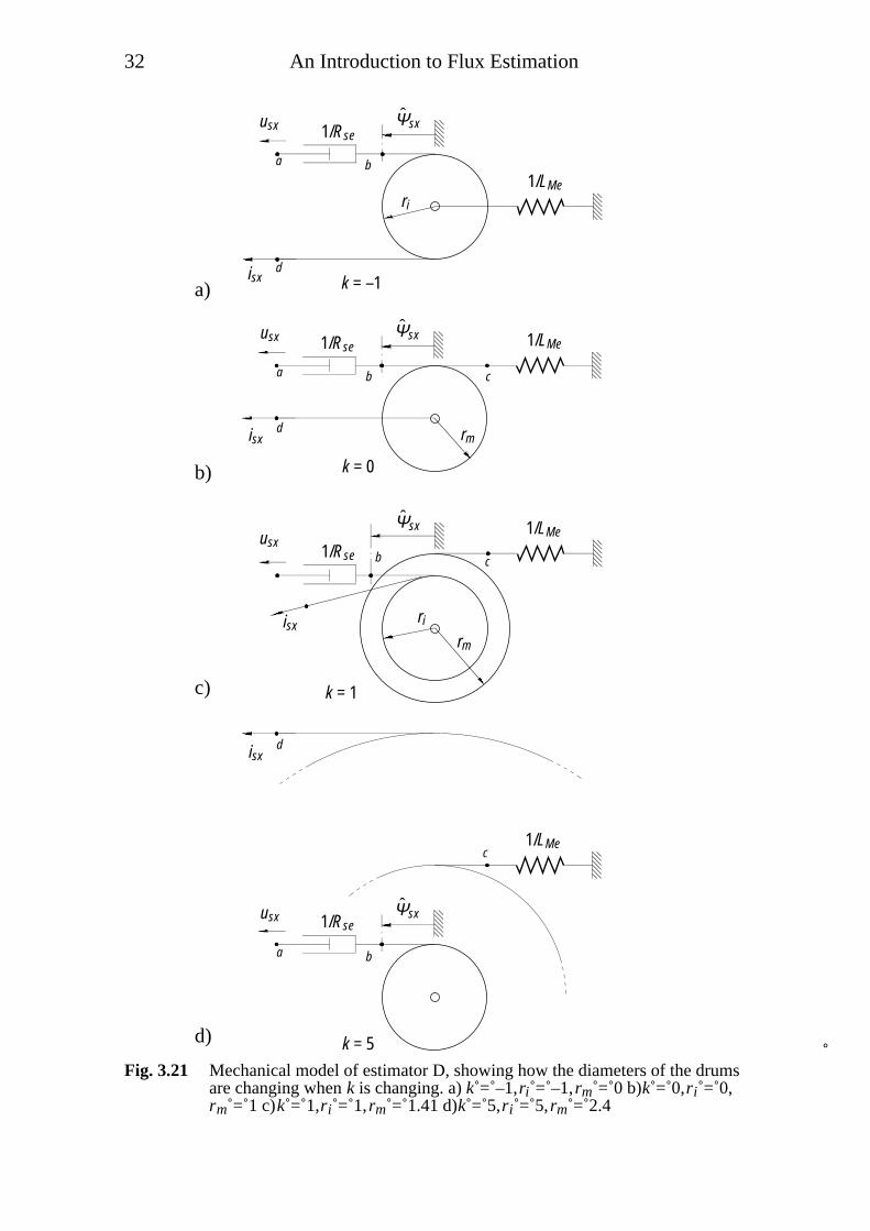
Fig. 3.21 Mechanical model of estimator D, showing how the diameters of the drums
are changing when k is changing. a) k = –1, ri = –1, rm = 0 b) k = 0, ri = 0,rm = 1 c) k = 1, ri = 1, rm = 1.41 d) k = 5, ri = 5, rm = 2.4

An Introduction to Flux Estimation 33
In Fig. 3.21 a), the gain is k = –1 corresponding to estimator A. The radiusof the magnetizing inductance drum rm is zero, and we have themechanical observer shown in Fig. 3.16, with point b drifting either to theleft or right at low frequencies if the resistance parameter is not perfectlymatched with the true resistance.
In Fig. 3.21 b), the gain is k = 0. Now the radius of the current drum iszero, and we have estimator C, which does not use the measured current.
As k is increased, the radius of the current drum ri = k is increased, and theinfluence of the measured current is increased. In Fig. 3.21 c), k = 1, whichgives a good balance of the trust put into measured current and measuredvoltage. However, good balance is a relative measure, and noise inmeasurements and estimator parameter errors are factors that must beregarded in an actual application.
As k is further increased, the influence of the measured voltage and thestator resistance parameter errors is decreased, as the levers for the currentand for the magnetizing inductance both are becoming dominant. This isseen in Fig. 3.21 d). Neither the equations, the block diagram of theobserver nor this mechanical model will tell at a first glance what ishappening at a large gain.
A second mechanical model shown in Fig. 3.22 can be derived whichclearly illustrates the behaviour when k is large. The drawback of thesecond model is that it will not work at k = –1. The ends of the viscousdamper representing stator resistance are attached to wires wrapped aroundtwo drums of radius rs, the radius of the current drum is ri , while the radiusof both the magnetizing inductance drum and the stator voltage drum isequal to 1.
ri
rs
1
a
d
e
rs
1
b c
va = usx
x = Ψsx
kMe = 1/LMedse = 1/Rse
ˆ
Fd = isx
ˆ
Fig. 3.22 Alternative mechanical model of estimator D, k = 0.5.
The equations for the mechanical system are

34 An Introduction to Flux Estimation
dx
dt= ve
vb = varsvc = vers
Fb = Fc = dse vb − vc( )Fe = k Mex
Fcrs + Fdri = Fe ⋅1
(3.30)
giving
dx
dt= va + ri
rs2
1
dse
Fd − k Me
dse
x1
rs2
(3.31)
This equation turns into equation (3.32) when the mechanical quantities arereplaced by electrical quantities,
dΨsx
dt= usx + ri
rs2
Rseisx − Rse
L Me
Ψsx1
rs2
(3.32)
This is equivalent to equation (3.17) if
rs = 1
1 + k(3.33)
and
ri = k
1 + k(3.34)
As k is increased, the radii of the viscous damper drums rs go towards zero,and the radius of the current drum goes towards 1. It is seen that the statorvoltage and stator resistance no longer have much influence on theestimated flux, while the stator current force is acting directly on themagnetizing inductance spring. This means that when k is increased, theobserver will behave more and more like estimator B shown in Fig. 3.17.Fig. 3.23 shows the observer at k = 5.
It is important to notice that there are no extra simplifications involved inthese mechanical models. The equations describing the mechanical systemsare both identical to the observer equation (3.17).

An Introduction to Flux Estimation 35
ri
usx
Ψsx
1/LMe
a
ˆ
isxd
e
rs
1/Rse
b crs
k = 5
Fig. 3.23 Alternative mechanical model of estimator D, k = 5.
As summarized in Table 3.1, the estimators A, B and C are all special casesof estimator D.
k estimator
–1 A
∞ B
0 C
Table 3.1 Relation between estimator D and estimators A, B and C.
The general observations on the observers assuming zero rotor current arevalid also for the complete observer where the rotor current no longer isassumed to be zero. With this basic knowledge of a flux observer, thecomplete flux observer can now be studied.

4Flux Observer Models
All the characteristics of the observers in Chapter 3, like noise sensitivityand parameter sensitivity, are valid also for a complete observer. However,new problems such as non-linearities arise when the rotor current no longeris assumed to be zero.
In this chapter it is assumed that the rotor speed ω is measured. In Chapter5, estimators without speed sensors are studied.
An observer for both stator and rotor flux can be obtained in the same wayas the simplified observer described by equation (3.13).
Again, the identity observer in equation (3.12) is the starting point for theflux observer. An observer for the induction machine described byequations (2.9)-(2.14), will take the form
dx
dt= A ex + Beu + K y − Cex( ) (4.1)
where
x = Ψ =
ÁÁs
ÁÁr
(4.2)
y = is (4.3)
u = us (4.4)
A e ω( ) =−Rse
1
L Me
+ 1
L Le
Rse
L Le
R re
L Le
−R re
L Le
+ jzpω
(4.5)
Be =1
0
(4.6)

Flux Observer Models 37
Ce = 1
L Me
+ 1
L Le
−1
L Le
(4.7)
K =Ks
Kr
(4.8)
A key to make this observer easy to tune, is to make the observer gainsdimensionless, which is done with the relation
K = Re k (4.9)
where
k =ks
kr
=ksx + j ksy
k rx + j k ry
(4.10)
and
Re =Rse 0
0 R re
(4.11)
The observer in matrix notation takes the form
dΨdt
= A eΨ + Beus + Rek is − CeΨ( ) (4.12)
This equation consists of two complex differential equations, one for theestimated stator flux,
dÁÁs
dt= us − Rse 1 + ks( ) is − ks is( ) (4.13)
and one for the estimated rotor flux
dÁÁr
dt= jzp ω ÁÁr − R re ir (4.14)
where
is = ÁÁs
L Me
− ÁÁr − ÁÁs
L Le
(4.15)
38 Flux Observer Models
ir = kr is − is( ) + ÁÁr − ÁÁs
L Le
(4.16)
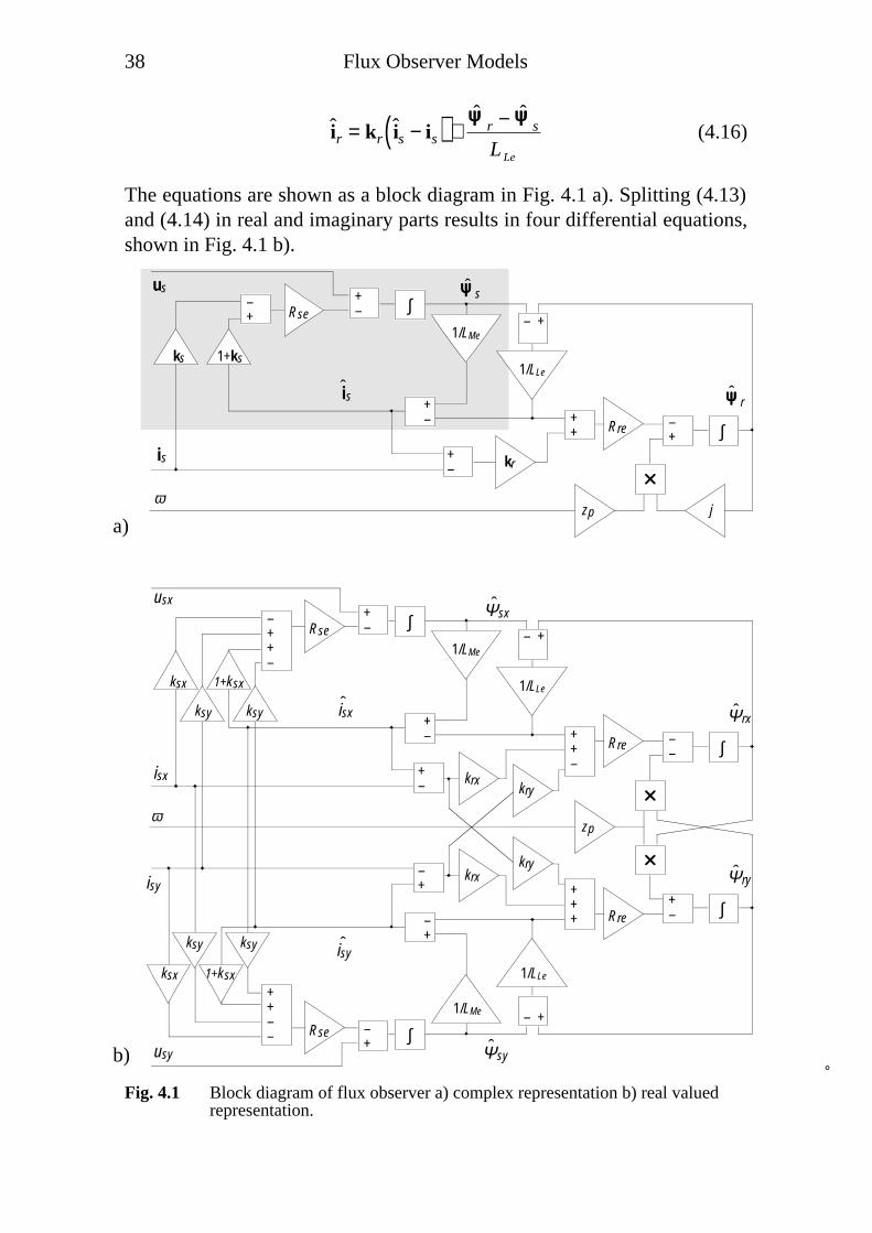
The equations are shown as a block diagram in Fig. 4.1 a). Splitting (4.13)and (4.14) in real and imaginary parts results in four differential equations,shown in Fig. 4.1 b).
1/LMe
isˆ
Rse–+
+–
ks 1+ks
∫– +
1/LLe
+– +
+ Rre –+ ∫
zp j
kr+–
ω
Ψsxˆ
1/LMe
isxˆ
Rse–++–
+–
ksx 1+ksx
∫
1/LLe
+– +
+–
Rre –– ∫
zp
krx+–
isx
usx
ω
Ψrxˆ
Ψsyˆ
1/LMe
isyˆ
Rse
++–– –
+ ∫
+ –1/LLe
–+
+++ Rre
+– ∫
krx–+isy
usy
Ψryˆ
ˆus
ˆ
ÁÁÁÁs
ÁÁÁÁr
is
kry
kry
ksyksy
ksx 1+ksx
ksyksy
– +
– +
b)
a)
Fig. 4.1 Block diagram of flux observer a) complex representation b) real valued
representation.

Flux Observer Models 39
The upper left corner (shaded) is basically the same as the block diagram ofthe observer in Fig. 3.11, where the rotor current is assumed to be zero.
Settling Time
One major difference between the simplified observer of Chapter 3, wherethe rotor current was zero, and the complete observer, is that the rotorspeed ω appears in the equations of the complete observer. First, thismakes the observer a non-linear system if ω is varying. Second, the rotorspeed must be measured or estimated in order to get an accurate fluxestimate. Speed estimation will be discussed in Chapter 5. In this chapter, itis assumed that the speed is measured perfectly.
The non-linearities affect the settling time of the observer. An observerwith zero gain will be used as a first example to demonstrate how thesettling time varies with ω. Fig. 4.2 shows a simulation of the error in theestimate of stator flux amplitude. The amplitude of the actual stator flux isconstant during the simulation, while the observer starts from zero.
-0.5
0
0.5
1
0 0.005 0.01 0.015 0.02 0.025 0.03
f1=50 Hz
t [s]
abs(
psis
)-ab
s(ps
isha
t)
-0.5
0
0.5
1
0 0.05 0.1 0.15 0.2 0.25 0.3
f1=5 Hz
t [s]
abs(
psis
)-ab
s(ps
isha
t)
Ψs – Ψs[Vs]
ˆ
Ψs – Ψs[Vs]
ˆ
t [s]
t [s]
f1 = 5 Hz
f1 = 50 Hz
Fig. 4.2 Settling time at 50 Hz and 5 Hz for observer with zero gain.
The motor is running at rated torque and at a stator frequency of 50 Hz inthe upper diagram and 5 Hz in the lower one. Note the different time scalesin the two diagrams. The vertical lines at 0.02 seconds and 0.2 seconds

40 Flux Observer Models
respectively, correspond to the time instants when the stator flux hascompleted one turn.
The diagrams show a very important property: The observer with gaink = 0 is ten times faster at 50 Hz than at 5 Hz. However, if the settling timeis measured in stator flux revolutions instead of seconds, the observer isalmost equally fast at both frequencies. It takes about one revolution forerrors in the estimates to reach zero in both cases.
The settling time can be reduced with an appropriate selection of the gainparameters. In Fig. 4.3, the same observer gain k is used at 50 Hz and 5 Hz.The response is faster than in Fig. 4.2, but it is still approximately 10 timesfaster at 50 Hz than at 5 Hz.
-0.5
0
0.5
1
0 0.005 0.01 0.015 0.02 0.025 0.03
f1=50 Hz
t [s]
abs(
psis
)-ab
s(ps
isha
t)
-0.5
0
0.5
1
0 0.05 0.1 0.15 0.2 0.25 0.3
f1=5 Hz
t [s]
abs(
psis
)-ab
s(ps
isha
t)
Ψs – Ψs[Vs]
ˆ
Ψs – Ψs[Vs]
ˆ
t [s]
t [s]
f1 = 5 Hz
f1 = 50 Hz
Fig. 4.3 Settling time at 50 Hz and 5 Hz. The same gain
k = 1.3 − 51j − 30 + 85 j[ ]T is used at both frequencies.
Pole placement (Åström et al, 1984) is a technique that can be used to setthe settling time of the observer. The observer poles are the eigenvalues ofthe matrix A e − RekCe( ) in equation (4.12). If the two complex poles of acomplex 2 × 2 matrix are denoted p1 and p2 the characteristic polynomialof the observer can be written
P s( ) = s2 + c1s + c2 = s2 − p1 + p2( )s + p1p2 (4.17)

Flux Observer Models 41
The required observer gain for desired observer poles is given by
k = Re−1P A e( )Wo
−1 0
1
= Re−1 A e
2 − p1 + p2( )A e + p1p2I( )Wo−1 0
1
(4.18)
where Wo is the observability matrix,
Wo =Ce
CeA e
(4.19)
Equation (4.18) is evaluated in Appendix E. Unfortunately, the expressionsare too complicated to be of much practical use. Note that the two poles donot have to be conjugates, as the 2 × 2 matrix is complex.
As matrix A e is varying with rotor speed ω, the observer gain must varywith speed if the poles are held constant. Fig. 4.4 shows a simulation at 50Hz and 5 Hz, with the same poles at both frequencies. This means thatdifferent gain parameters k are used at the two frequencies.
-0.5
0
0.5
1
0 0.005 0.01 0.015 0.02 0.025 0.03
f1=50 Hz
t [s]
abs(
psis
)-ab
s(ps
isha
t)
-4
-3
-2
-1
0
1
0 0.005 0.01 0.015 0.02 0.025 0.03
f1=5 Hz
t [s]
abs(
psis
)-ab
s(ps
isha
t)
Ψs – Ψs[Vs]
ˆ
Ψs – Ψs[Vs]
ˆ
t [s]
t [s]
f1 = 5 Hz
f1 = 50 Hz
Fig. 4.4 Settling time at 50 Hz and 5 Hz. The poles are placed in –1500 when the
observer is operating both at 50 Hz and 5 Hz. The gain is
k = 1.3 − 51j − 30 + 85 j[ ]T at 50 Hz and k = [481 + 579 j 793 + 996 j]T at
5 Hz.
42 Flux Observer Models
Note that the same time scale is used in the 50 Hz and 5 Hz diagrams. Asthe poles are the same for the two cases, we have the same response time.The two curves look different because it is the amplitude error Ψs − Ψs thatis shown, not the actual states of the observer.
At a first look, pole placement seems to be a useful technique formanipulating the dynamic behaviour of the observer. However, the price ishigh for a fast observer at a low frequency. The parameters of the gainvector k must be increased between 10 and 400 times in order to make theobserver as fast at 5 Hz as it is at 50 Hz. Such a high gain is usually notrecommendable due to noise sensitivity. The conclusion is that with poleplacement, control of the gain vector is lost, and the gain might increasebeyond reasonable limits.
The settling time is not the most critical factor of an observer. Usually, theobserver flux tracks the flux of the induction machine, and the situationwhen there is nominal flux in the machine and the observer flux is zero is arare case. More important is the sensitivity to errors in parameters, whichwill be discussed later in this chapter.
Poles in Different Reference Frames
Another problem with pole placement is that the choice of reference framewill affect the location of the poles. Two observers in different referenceframes, with identical behaviour, will not have the same poles. Why thepoles differ in different reference frames is further evaluated in AppendixG. Until now, both the induction machine and the observer have beendescribed in a stator oriented stationary reference frame. They might aswell be described in a rotating reference frame, rotating with the angularfrequency ωk. If the observer’s frame is rotating with the same frequency asthe frequency of the stator voltage vector,
ωk = ω1 (4.20)
the estimated stator and rotor flux vectors will be constant, instead ofrotating, when the induction machine is running at constant speed andconstant torque. This observer is described by
dΨ r
dt= A e − jω1 I( )Ψ r + Beus
r + Rek isr − CeΨ
r( ) (4.21)

Flux Observer Models 43
where the r-superscript denotes vectors in the rotating reference frame1,and
Ψ r = Ψ e− jω1t
⇔
Ψ = Ψ r e jω1t
(4.22)
usr = us e− jω1t (4.23)
isr = is e− jω1t (4.24)
If the gain k is the same in the observers of equation (4.12) and equation(4.21), they will have identical behaviour, meaning that Ψ of the firstobserver will be identical to Ψ r e jω1t of the second observer. However, thepoles of the first observer (see Appendix E) are the eigenvalues ofA e − Re k Ce( ), while the poles of the second observer are the eigenvalues
of A e − Re k Ce − jω1 I( ). Fig. 4.5 shows the poles of both observers.
-300
-200
-100
0
100
200
300
-300 -200 -100 0 100 200 300
x
x
*
*
k=[-0.5;0], x: wk=0, *: wk=2*pi*50
stationaryreference frame
rotatingreference frame
k = [0.5 0]T, 50 Hz, nominal speed
ℑ (s)
ℜ (s)
Fig. 4.5 ’x’ marks the poles of the observer in a stationary reference frame and ’*’marks the poles of the observer in a reference frame rotating with angularfrequency ω1 = 2π f1 = 2π50 ≈ 314 rad / s
1 the r-superscript is sometimes used in the literature for a rotor oriented reference frame.

44 Flux Observer Models
Note that the real parts of the poles of both observers are equal, while thedifference in the imaginary parts is equal to ω1. It must also be pointed outthat the observer is a non-linear system. Poles in the left half planeguarantee stability only in a linear system. An example of this is given inAppendix G.
Parameter Sensitivity
It is important to have as accurate observer parameters as possible, in orderto get accurate estimates. Various methods for parameter identificationexist (Zai et al, 1992, Krzeminski, 1991 and Vélez-Reyes et al, 1995), butwill not be further discussed here. Instead, the influence of parameter errorswill be studied.
The observer structure described by equation (4.12) is sometimes criticizedfor its parameter sensitivity at low frequencies (Jansen et al, 1994a). This isa misunderstanding due to its similarities to estimator A with poor lowfrequency properties, but with a proper choice of the gain k, this estimatorwill behave like anything from estimator A to estimator C. With a suitablegain, this observer will work well in its entire frequency range.
It is difficult to derive analytic expressions for the parameter sensitivity.Instead, the flux estimate errors at different frequencies are calculated for acertain motor, and compared with the errors of an observer described byJansen et al (1994a).
As the flux vectors are rotating, the errors in the stator flux and rotor flux,
ÁÁs = ÁÁs − ÁÁs (4.25)
and
ÁÁr = ÁÁr − ÁÁr (4.26)
will also be rotating vectors. The relative errors in flux magnitude andphase are better measures. Here, the magnitude of the estimated fluxrelated to the actual flux
ÁÁs
ÁÁs
= Ψs
Ψs
(4.27)
and the error in phase,

Flux Observer Models 45
arg ÁÁs( ) − arg ÁÁs( ) = ϕs − ϕs (4.28)
will be studied.
These measures will be constant if the machine and observer are runningwith flux of constant magnitude and constant angular velocity. To calculatethe steady state2 flux of the observer, the following relation can be used,
dΨdt
= jω1 Ψ (4.29)
where
ω1 = 2 π f1 (4.30)
and f1 is the frequency of the stator voltage. Equation (4.12) combined withequations (4.29) and (2.10) give
jω1 Ψ = A eΨ + Beus + Rek CΨ − CeΨ( ) (4.31)
or
A e − RekCe − jω1 I( )Ψ = −Beus − RekCΨ (4.32)
where Ae, Be and Ce are given by (4.5), (4.6) and (4.7), respectively.
The steady state flux estimate can now be calculated as
Ψ = − A e − RekCe − jω1 I( )−1Beus + RekCΨ( ) (4.33)
and the steady state flux of the motor is given by
Ψ = − A − jω1 I( )−1B us (4.34)
Parameter Sensitivity Comparison Between Two Observers
The error of the flux estimate in equation (4.33) will be compared to theflux estimate of an observer described by Jansen et al (1994a), shown hereas a block diagram in Fig. 4.6. This observer was chosen as referencebecause of its good properties both at low and high frequencies.
2 The term ”steady state” will be used even though the flux vectors are rotating. The term will be usedwhen the magnitude and the angular velocity of the flux vectors are constant.

46 Flux Observer Models
–+
Rse σe Lse
++
–+ Lre /Lme+
+K1
K2
+–
∫++–
1/τre
Lme /τre
zp
λrcˆ
λsˆ
λ
λr kγˆis
us
ω
∫
∫
j
Fig. 4.6 Block diagram of λ-observer.
With the notation used by Jansen et al (1994a), this observer is describedby
d¬¬s
dt= −K1
L re
Lme
¬¬s+K1¬¬ rc+K2¬¬+ σeLseL re
Lme
K1 − Rse
is + us
d¬¬ rc
dt= −¬¬ rc
1
τre
− jzp ω
+ 1
τre
Lmeis
d¬¬dt
= − L re
Lme
¬¬s+¬¬ rc+σeLseL re
Lme
is
(4.35)
where ¬¬s is the estimated stator flux and ¬¬ rc and ¬¬ are intermediate states.In matrix notation the observer is described by
Flux Observer Models 47
dλdt
= A λe λ + Bλe
is
us
=
−K1L re
Lme
K1 K2
0 − 1
τre
− jzp ω
0
− L re
Lme
1 0
λ +
σeLseL re
Lme
K1 − Rse 1
1
τre
Lme 0
σeLseL re
Lme
0
is
us
(4.36)
where
λ =¬¬s
¬¬ rc
¬¬
(4.37)
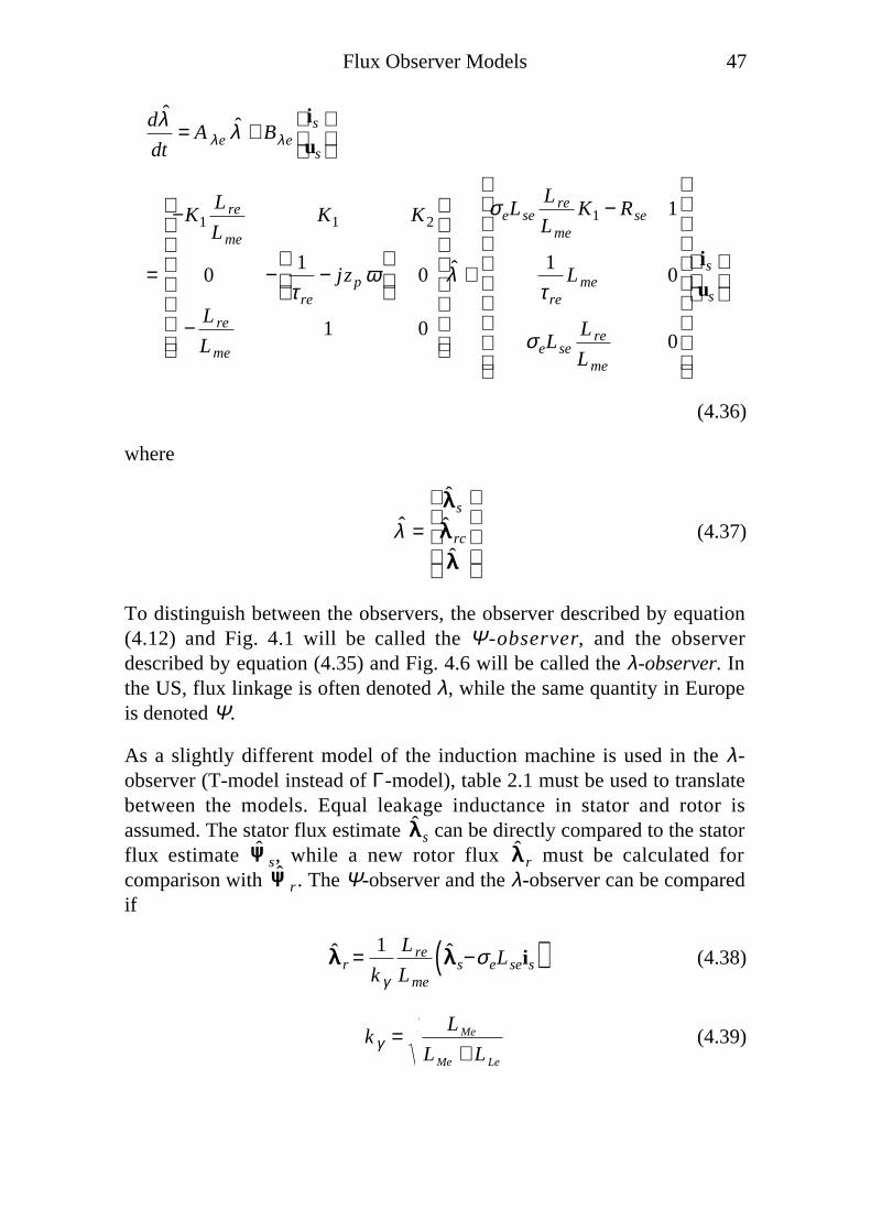
To distinguish between the observers, the observer described by equation(4.12) and Fig. 4.1 will be called the Ψ-observer, and the observerdescribed by equation (4.35) and Fig. 4.6 will be called the λ-observer. Inthe US, flux linkage is often denoted λ, while the same quantity in Europeis denoted Ψ.
As a slightly different model of the induction machine is used in the λ-observer (T-model instead of Γ-model), table 2.1 must be used to translatebetween the models. Equal leakage inductance in stator and rotor isassumed. The stator flux estimate ¬¬s can be directly compared to the statorflux estimate ÁÁs, while a new rotor flux ¬¬ r must be calculated forcomparison with ÁÁr . The Ψ-observer and the λ-observer can be comparedif
¬¬ r = 1
k γ
L re
Lme
¬¬s−σeLseis( ) (4.38)
k γ = L Me
L Me + L Le
(4.39)

48 Flux Observer Models
Lme = k γ L Me = L Me
L Me
L Me + L Le
(4.40)
Lse = Lme + Lsle = L Me (4.41)
L re = Lse (4.42)
σe = 1 − Lme2
L reLse
(4.43)
τre = L re
R rek γ2
(4.44)
ϑs = arg ¬¬s( ) (4.45)
The steady state value of λ (actually the value when the magnitude andangular velocity of the components are constant) is given by
λ = − A λe − jω1 I( )−1Bλe
is
us
(4.46)
The idea behind this heuristic observer is to combine the good properties ofestimators similar to estimator A and estimator C of Chapter 3. The leftpart of the observer in Fig. 4.6, the current model, depends on themeasured current and works well at low frequencies. The right part, thevoltage model, is integrating the measured voltage, with good results athigh frequencies. At low frequencies, the estimated flux of the currentmodel is correcting the flux of the voltage model, while at higherfrequencies, the influence of the current model is reduced. The breakfrequency where the observer makes a transition from the current model tothe voltage model can be set by the gain parameters K1 and K2 in equation(4.35). The parameters can be calculated from the chosen bandwidth of theobserver, governed by the real eigenvalues –σ1 and –σ2. Having selectedthe bandwidth, the gains are given by
K1 = Lme
L re
σ1 + σ2( ) (4.47)
and

Flux Observer Models 49
K 2 = Lme
L re
σ1σ2 (4.48)
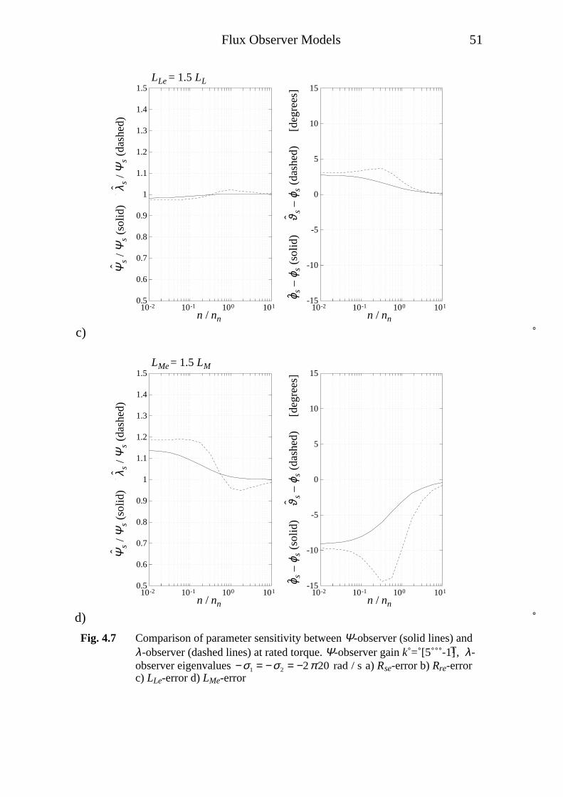
The λ-observer and Ψ-observer are compared in Fig. 4.7 and Fig. 4.8. Thegain of the Ψ-observer is k = [5 – 1]T . This gain was chosen empirically,mainly to get a good balance between parameter sensitivity and noisesensitivity.
The eigenvalues of the λ-observer are −σ1 = −σ2 = −2π 20 rad / s.
Fig. 4.7 shows the error at rated torque when the rotor speed is slowlyvaried from 1% of the rated speed up to 10 times the rated speed. The solidlines represent the amplitude of the estimated flux of the Ψ-observerrelated to the actual flux, Ψs Ψs , and its phase error, ϕs − ϕs. The dashedlines show the corresponding measures of the λ -observer, λs Ψs andϑs − ϕs.
It is seen that the errors in estimates of the Ψ-observer are smaller in mostcases, except for the case shown in Fig. 4.7 a), where there is an error inRse.
In Fig. 4.8, the two observers are compared again, now at varying slip andload torque. Also in this case, the errors are smaller for the Ψ-observer thanfor the λ-observer.
If the bandwidth of the λ-observer is increased, the sensitivity to errors inthe stator resistance is reduced, because more trust is put into the currentmodel which is completely insensitive to stator resistance error. However,higher bandwidth will accentuate errors due to errors in the other para-meters at low frequencies. The bandwidth given by σ1 = σ2 = 2 π 20 rad/swas selected as a good compromise.

50 Flux Observer Models
a)
0.5
0.6
0.7
0.8
0.9
1
1.1
1.2
1.3
1.4
1.5
10-2 10-1 100 101
n/nn
abs(
psir
hat/p
sir)
motor: imep, k=[-5; -1]
-15
-10
-5
0
5
10
15
10-2 10-1 100 101
n/nn
arg(
psir
hat/p
sir)
deg
rees
Rso=1.5*Rs
ϕ s –
ϕs
(sol
id)
ϑ
s –
ϕ s (
dash
ed)
[
degr
ees]
ˆˆ
Ψs
/ Ψs
(sol
id)
λ
s / Ψ
s (d
ashe
d)ˆ
ˆ
n / nn
Rse = 1.5 Rs
n / nn
b)
0.5
0.6
0.7
0.8
0.9
1
1.1
1.2
1.3
1.4
1.5
10-2 10-1 100 101
n/nn
abs(
psir
hat/p
sir)
motor: imep, k=[-5; -1]
-15
-10
-5
0
5
10
15
10-2 10-1 100 101
n/nn
arg(
psir
hat/p
sir)
deg
rees
RRo=1.5*RR
ϕ s –
ϕs
(sol
id)
ϑ
s –
ϕ s (
dash
ed)
[
degr
ees]
ˆˆ
Ψs
/ Ψs
(sol
id)
λ
s / Ψ
s (d
ashe
d)ˆ
ˆ
n / nn
Rre = 1.5 Rr
n / nn
Flux Observer Models 51
c)
0.5
0.6
0.7
0.8
0.9
1
1.1
1.2
1.3
1.4
1.5
10-2 10-1 100 101
n/nn
abs(
psir
hat/p
sir)
motor: imep, k=[-5; -1]
-15
-10
-5
0
5
10
15
10-2 10-1 100 101
n/nn
arg(
psir
hat/p
sir)
deg
rees
LLo=1.5*LL
ϕ s –
ϕs
(sol
id)
ϑ
s –
ϕ s (
dash
ed)
[
degr
ees]
ˆˆ
Ψs
/ Ψs
(sol
id)
λ
s / Ψ
s (d
ashe
d)ˆ
ˆ
n / nn
LLe = 1.5 LL
n / nn
d)
0.5
0.6
0.7
0.8
0.9
1
1.1
1.2
1.3
1.4
1.5
10-2 10-1 100 101
n/nn
abs(
psir
hat/p
sir)
motor: imep, k=[-5; -1]
-15
-10
-5
0
5
10
15
10-2 10-1 100 101
n/nn
arg(
psir
hat/p
sir)
deg
rees
LMo=1.5*LM
ϕ s –
ϕs
(sol
id)
ϑ
s –
ϕ s (
dash
ed)
[
degr
ees]
ˆˆ
Ψs
/ Ψs
(sol
id)
λ
s / Ψ
s (d
ashe
d)ˆ
ˆ
n / nn
LMe = 1.5 LM
n / nn
Fig. 4.7 Comparison of parameter sensitivity between Ψ-observer (solid lines) andλ-observer (dashed lines) at rated torque. Ψ-observer gain k = [5 -1]T, λ-observer eigenvalues −σ1 = −σ2 = −2π 20 rad / s a) Rse-error b) Rre-errorc) LLe-error d) LMe-error

52 Flux Observer Models
a)
0.5
0.6
0.7
0.8
0.9
1
1.1
1.2
1.3
1.4
1.5
0 0.05 0.1
slip
abs(
psir
hat/p
sir)
motor: imep, k=[-5; -1]
-15
-10
-5
0
5
10
15
0 0.05 0.1
slip
arg(
psir
hat/p
sir)
deg
rees
Rso=1.5*Rs
ϕ s –
ϕs
(sol
id)
ϑ
s –
ϕ s (
dash
ed)
[
degr
ees]
ˆˆ
Ψs
/ Ψs
(sol
id)
λ
s / Ψ
s (d
ashe
d)ˆ
ˆ
Rse = 1.5 Rs
slip s slip s
b)
0.5
0.6
0.7
0.8
0.9
1
1.1
1.2
1.3
1.4
1.5
0 0.05 0.1
slip
abs(
psir
hat/p
sir)
motor: imep, k=[-5; -1]
-15
-10
-5
0
5
10
15
0 0.05 0.1
slip
arg(
psir
hat/p
sir)
deg
rees
RRo=1.5*RR
ϕ s –
ϕs
(sol
id)
ϑ
s –
ϕ s (
dash
ed)
[
degr
ees]
ˆˆ
Ψs
/ Ψs
(sol
id)
λ
s / Ψ
s (d
ashe
d)ˆ
ˆ
Rre = 1.5 Rr
slip s slip s

Flux Observer Models 53
c)
0.5
0.6
0.7
0.8
0.9
1
1.1
1.2
1.3
1.4
1.5
0 0.05 0.1
slip
abs(
psir
hat/p
sir)
motor: imep, k=[-5; -1]
-15
-10
-5
0
5
10
15
0 0.05 0.1
slip
arg(
psir
hat/p
sir)
deg
rees
LLo=1.5*LL
ϕ s –
ϕs
(sol
id)
ϑ
s –
ϕ s (
dash
ed)
[
degr
ees]
ˆˆ
Ψs
/ Ψs
(sol
id)
λ
s / Ψ
s (d
ashe
d)ˆ
ˆ
LLe = 1.5 LL
slip s slip s
d)
0.5
0.6
0.7
0.8
0.9
1
1.1
1.2
1.3
1.4
1.5
0 0.05 0.1
slip
abs(
psir
hat/p
sir)
motor: imep, k=[-5; -1]
-15
-10
-5
0
5
10
15
0 0.05 0.1
slip
arg(
psir
hat/p
sir)
deg
rees
LMo=1.5*LM
ϕ s –
ϕs
(sol
id)
ϑ
s –
ϕ s (
dash
ed)
[
degr
ees]
ˆˆ
Ψs
/ Ψs
(sol
id)
λ
s / Ψ
s (d
ashe
d)ˆ
ˆ
LMe = 1.5 LM
slip s slip s
Fig. 4.8 Comparison of parameter sensitivity between Ψ-observer (solid lines) andλ-observer (dashed lines) at varying slip and torque. Ψ-observer gaink = [5 -1]T, λ-observer eigenvalues −σ1 = −σ2 = −2π 20 rad / s a) Rse-error b) Rre-error c) LLe-error d) LMe-error

54 Flux Observer Models
a)
0.5
0.6
0.7
0.8
0.9
1
1.1
1.2
1.3
1.4
1.5
10-2 10-1 100 101
n/nn
abs(
psir
hat/p
sir)
motor: imep, k1=[-5; 0], k2=[0; 0]
-15
-10
-5
0
5
10
15
10-2 10-1 100 101
n/nn
arg(
psir
hat/p
sir)
deg
rees
Rso=1.5*Rs
ϕ s –
ϕs
[deg
rees
]ˆ
Ψs
/ Ψs
ˆ
n / nn
Rse = 1.5 Rs
n / nn
k = [5 0]T (solid)
k = [0 0]T (dashed)
k = [5 0]T (solid)
k = [0 0]T (dashed)
b)
0.5
0.6
0.7
0.8
0.9
1
1.1
1.2
1.3
1.4
1.5
10-2 10-1 100 101
n/nn
abs(
psir
hat/p
sir)
motor: imep, k1=[-5; 0], k2=[0; 0]
-15
-10
-5
0
5
10
15
10-2 10-1 100 101
n/nn
arg(
psir
hat/p
sir)
deg
rees
RRo=1.5*RR
ϕ s –
ϕs
[deg
rees
]ˆ
Ψs
/ Ψs
ˆ
n / nn
Rre = 1.5 Rr
n / nn
k = [5 0]T (solid)
k = [0 0]T (dashed)
k = [5 0]T (solid)
k = [0 0]T (dashed)

Flux Observer Models 55
c)
0.5
0.6
0.7
0.8
0.9
1
1.1
1.2
1.3
1.4
1.5
10-2 10-1 100 101
n/nn
abs(
psir
hat/p
sir)
motor: imep, k1=[-5; 0], k2=[0; 0]
-15
-10
-5
0
5
10
15
10-2 10-1 100 101
n/nn
arg(
psir
hat/p
sir)
deg
rees
LLo=1.5*LL
ϕ s –
ϕs
[deg
rees
]ˆ
Ψs
/ Ψs
ˆ
n / nn
LLe = 1.5 LL
n / nn
k = [5 0]T (solid)
k = [0 0]T (dashed)
k = [5 0]T (solid)
k = [0 0]T (dashed)
d)
0.5
0.6
0.7
0.8
0.9
1
1.1
1.2
1.3
1.4
1.5
10-2 10-1 100 101
n/nn
abs(
psir
hat/p
sir)
motor: imep, k1=[-5; 0], k2=[0; 0]
-15
-10
-5
0
5
10
15
10-2 10-1 100 101
n/nn
arg(
psir
hat/p
sir)
deg
rees
LMo=1.5*LM
ϕ s –
ϕs
[deg
rees
]ˆ
Ψs
/ Ψs
ˆ
n / nn
LMe = 1.5 LM
n / nn
k = [5 0]T (solid)
k = [0 0]T (dashed)
k = [5 0]T (solid)
k = [0 0]T (dashed)
Fig. 4.9 Comparison of parameter sensitivity between Ψ-observers with gaink = [5 0]T (solid) and gain k = [0 0]T (dashed). a) Rse-error b) Rre-error c)LLe-error d) LMe-error

56 Flux Observer Models
a)
0.5
0.6
0.7
0.8
0.9
1
1.1
1.2
1.3
1.4
1.5
10-2 10-1 100 101
n/nn
abs(
psir
hat/p
sir)
motor: imep, k1=[-5; 0], k2=[-5; -1]
-15
-10
-5
0
5
10
15
10-2 10-1 100 101
n/nn
arg(
psir
hat/p
sir)
deg
rees
Rso=1.5*Rs
ϕ s –
ϕs
[deg
rees
]ˆ
Ψs
/ Ψs
ˆ
n / nn
Rse = 1.5 Rs
n / nn
k = [5 0]T (solid)
k = [5 –1]T (dashed)
k = [5 0]T (solid)
k = [5 –1]T (dashed)
b)
0.5
0.6
0.7
0.8
0.9
1
1.1
1.2
1.3
1.4
1.5
10-2 10-1 100 101
n/nn
abs(
psir
hat/p
sir)
motor: imep, k1=[-5; 0], k2=[-5; -1]
-15
-10
-5
0
5
10
15
10-2 10-1 100 101
n/nn
arg(
psir
hat/p
sir)
deg
rees
RRo=1.5*RR
ϕ s –
ϕs
[deg
rees
]ˆ
Ψs
/ Ψs
ˆ
n / nn
Rre = 1.5 Rr
n / nn
k = [5 0]T (solid)
k = [5 –1]T (dashed)
k = [5 0]T (solid)
k = [5 –1]T (dashed)
Flux Observer Models 57
c)
0.5
0.6
0.7
0.8
0.9
1
1.1
1.2
1.3
1.4
1.5
10-2 10-1 100 101
n/nn
abs(
psir
hat/p
sir)
motor: imep, k1=[-5; 0], k2=[-5; -1]
-15
-10
-5
0
5
10
15
10-2 10-1 100 101
n/nn
arg(
psir
hat/p
sir)
deg
rees
LLo=1.5*LL
ϕ s –
ϕs
[deg
rees
]ˆ
Ψs
/ Ψs
ˆ
n / nn
LLe = 1.5 LL
n / nn
k = [5 0]T (solid)
k = [5 –1]T (dashed)
k = [5 0]T (solid)
k = [5 –1]T (dashed)
d)
0.5
0.6
0.7
0.8
0.9
1
1.1
1.2
1.3
1.4
1.5
10-2 10-1 100 101
n/nn
abs(
psir
hat/p
sir)
motor: imep, k1=[-5; 0], k2=[-5; -1]
-15
-10
-5
0
5
10
15
10-2 10-1 100 101
n/nn
arg(
psir
hat/p
sir)
deg
rees
LMo=1.5*LM
ϕ s –
ϕs
[deg
rees
]ˆ
Ψs
/ Ψs
ˆ
n / nn
LMe = 1.5 LM
n / nn
k = [5 0]T (solid)
k = [5 –1]T (dashed)
k = [5 0]T (solid)
k = [5 –1]T (dashed)
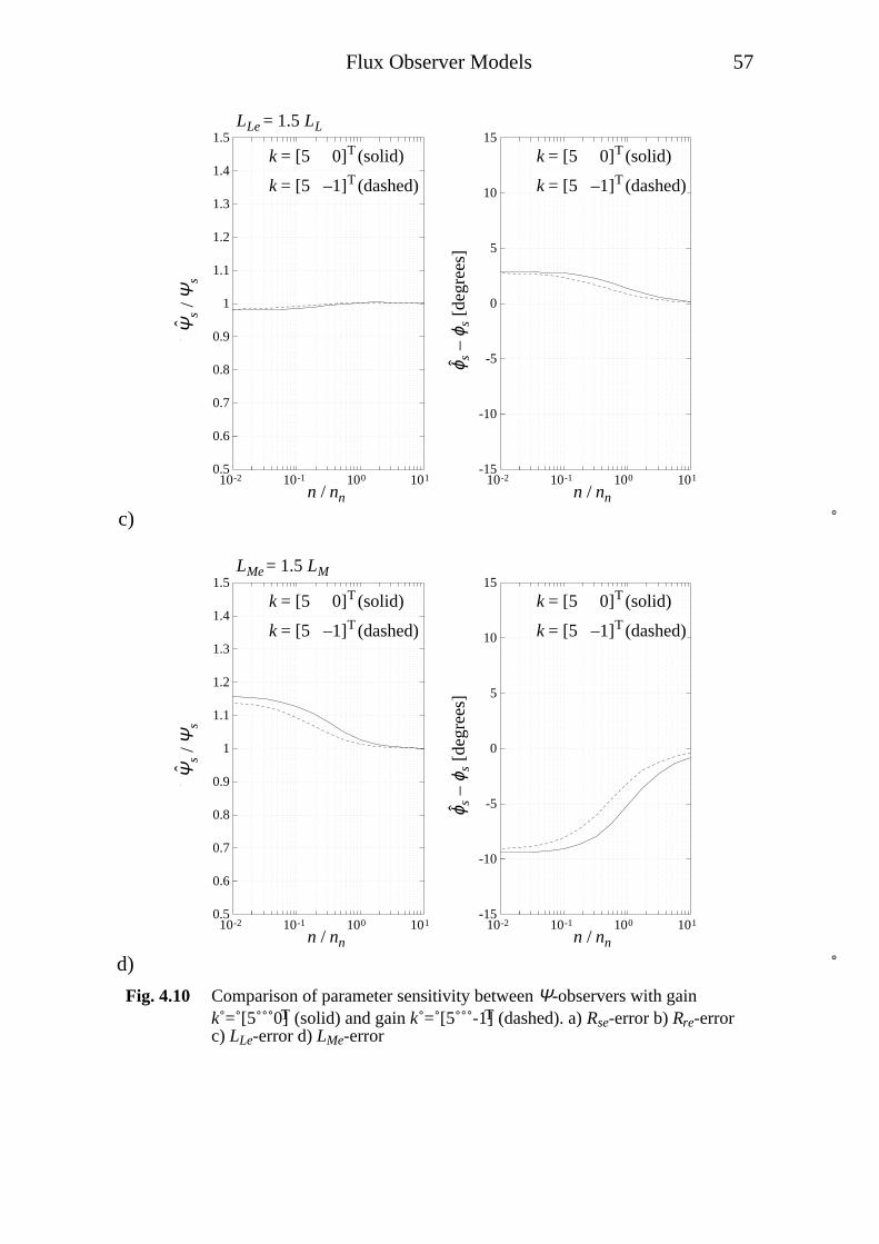
Fig. 4.10 Comparison of parameter sensitivity between Ψ-observers with gaink = [5 0]T (solid) and gain k = [5 -1]T (dashed). a) Rse-error b) Rre-errorc) LLe-error d) LMe-error

58 Flux Observer Models
Observer Gain Influence on Parameter Sensitivity
The gain vector k of the Ψ-observer will affect the parameter sensitivity ina more direct way than K1 and K2 of the λ-observer. At low and highfrequencies, the error of the λ-observer is not much affected by K1 and K2.At low frequency, the parameter sensitivity is the same as the parametersensitivity of the current model. At high frequencies, the sensitivity is thesame as the sensitivity of the voltage model. The gain k of the Ψ-observeron the other hand, will affect the parameter sensitivity in the entirefrequency range. The error of the Ψ-observer in Fig. 4.7 a) can be reducedby increasing the gain of the observer. In Fig. 4.9 and Fig. 4.10, the steadystate errors of the Ψ-observer is compared for different selections of thegain. In Fig. 4.9, the solid lines represent a gain of ks = 5 and k r = 0 ,while the dashed line represent an observer with zero gain.
In Fig. 4.9 it is seen that the error is smaller for ksx = 5 than for ksx = 0,comparable to the error reduction seen in Fig. 3.12 and Fig. 3.14. The errorcan be further reduced with k rx = −1 instead of k rx = 0, seen in Fig. 4.10.However, the effects of krx are less predictable than the effects of ksx andthe observer might be unstable at certain speeds if it is not chosen withgreat care. As the gain ksx has more influence on the steady state error thankrx, it is recommended to set krx = 0.
The imaginary parts of the observer gain, ksy and kry should also be zero forstability reasons. Both parameters will have different effects if the rotorspeed is positive or negative. If they are chosen so that the observer isstable for clockwise rotation, the observer will be unstable for counterclockwise rotation. If, for some reason ksy and kry, are given values otherthan zero, observer gain scheduling must be used, changing the signs of ksy
and kry when the direction of rotation is changed.
Flux Observer Conclusions
The parameter sensitivity of the observer structure shown in Fig. 4.1 can besignificantly reduced by selecting an appropriate observer gain. Thestructure with dimensionless observer gains makes the selection mucheasier. The gains rather than the poles of the observer should be heldconstant at varying speed. As a result, the response time of the observerwill be slower at lower frequencies. Although the sensitivity to errors in thestator resistance is reduced by using a large value of ks, the sensitivity tonoise is increased. Thus, it is important to have an as accurate parameterRse as possible. This is not a big drawback as the stator resistance is theeasiest parameter in the induction machine to measure.

5Speed Observer Models
In earlier chapters, it was assumed that rotor speed was measured, and thespeed signal was used as input to the flux observer. In this chapter, thespeed as well as the flux will be estimated instead of measured.
Two basic strategies for speed estimation are found in the literature; onestrategy uses the machine model in equations (2.3)-(2.6) together withmeasured current and voltage (Yang et al, 1993, Schauder, 1992, Tajima etal, 1993 and Jönsson, 1991). The other strategy relies on saliency withinthe machine. Unfortunately, both strategies are related with limitations.
The difficulty with the first strategy appears at low speeds and lowfrequencies. Even though it is not directly apparent from the machinemodel, the measured current and voltage carry no information on the speedif the frequency of the stator voltage is zero as will be shown later. Thisfact is seldom mentioned in the references. Instead, it is often stated thatthese methods fail at zero speed, not at zero frequency (Jansen et al, 1993).Extended Kalman filters have been tried to overcome the low frequencyproblems (von Westerholt et al, 1992b, Henneberger et al, 1991, Kim et al,1994), but it is obvious that none of these methods will work properlywhen speed information is not present in the measured signals.
The difficulty with the second strategy is that the rotor of the inductionmachine is smooth, and the ideal induction machine described by equations(2.3)-(2.6) has no saliency at all. In the actual machine, rotor slotting ispresent, resulting in current harmonics (Hurst et al, 1994, Beguenane et al,1994, Haemmerli, 1986 and Veltman, 1994). The FFT analysis required toextract the speed information from the harmonics is time consuming, andthe information is reduced at low speed and low frequency for this methodas well. A promising method is described by Schroedl (1992) that usessaliency introduced by local saturation of the magnetic flux paths instead.This method has also been reported to fail in the low speed region (Jansenet al, 1994a). To solve the low speed problems, a new method using amodified rotor with a modulation in the width of the slot openings has beenpresented (Jansen et al, 1994a). The main drawback of this method is that astandard induction machine cannot be used.

60 Speed Observer Models
The first strategy, using the machine model in equations (2.3)-(2.6), can beimplemented with standard induction machines and frequency inverterswith moderate additional hardware. Only this strategy will be studied here.
Introduction to Speed Estimation
In this section a simplified mechanical model will illustrate how the rotorspeed of the induction machine can be estimated, and also illustrate somerelated problems.
With some simplifications, the mechanical model in Fig. 5.1 is a modelanalogous to the torque producing part of the induction machine. In thismodel, rotational movement is replaced by linear movement and torque isreplaced by force. Note that the equilibrium position of the spring is atl = 0.
ul
k = d = a
v
mi
1Rs + Rr
1R
=1LL
Fload
Fig. 5.1 Simplified mechanical model illustrating induction machine speedestimation.
In the mechanical model in Appendix C, Fig. C.2, it is seen that the leakageinductance has the main influence in the tangential direction, the torqueproducing direction, while the magnetizing inductance can be neglected.The stator and rotor resistance can be considered connected in series. Thespring in Fig. 5.1 is representing the leakage inductance LL and the viscousdamper the sum of the stator resistance Rs and rotor resistance Rr. Themoment of inertia J is represented by the mass m. Estimating the speed v ofthe carriage is analogous to estimating the rotor speed ω of an inductionmachine.
The input to the system u is the speed of point a representing the tangentialpart of the stator voltage vector. The force i, representing the tangential partof the stator current vector is an output that can be measured. Fload isrepresenting the load torque and can not be measured.
According to the laws for a mechanical system described in Appendix B,the system in Fig. 5.1 is described by

Speed Observer Models 61
dl
dt= u − k
dl − v = u − R
L L
l − v (5.1)
dv
dt= k
ml − Fload
m= 1
m L L
l − Fload
m(5.2)
i = k l = 1
L L
l (5.3)
or in matrix notation
dx
dt= Ax + Bu + F (5.4)
y = Cu (5.5)
where
x =
l
v
(5.6)
y = i (5.7)
A =
−R
L−1
1
m L L
0
(5.8)
B =1
0
(5.9)
C = [1 / LL 0] (5.10)
F =0
Fload
(5.11)
If the load force is equal to zero, the velocity v of the carriage will be equalto the input u at steady state. This is analogous to an induction machinerunning at synchronous speed. If the load is greater than zero, the velocity vwill be less than u, comparable to a loaded induction machine running withslip. To conclude, estimating the velocity v is analogous to estimating the

62 Speed Observer Models
rotor speed ω of an induction machine with unknown load torque. Derivinga velocity observer for this mechanical system is the first step in derivingan observer for the rotor speed of the induction machine, which will bedone later in this chapter.
Velocity Observer, Approach 1
The identity observer structure in equation (3.12) cannot be applied directlyto this system because of the unknown input Fload in equation (5.2). A firstheuristic approach could simply be to integrate the error in an estimate ofthe force i, resulting in a velocity estimate, where the estimated force is aresult of the standard observer structure applied to equation (5.1). We have
dl
dt= u − R
L L
l − v + k1 i − i( ) (5.12)
i = 1
L L
l (5.13)
dv
dt= k 2 i − i( ) (5.14)
The velocity estimate v will be integrated until the errors in the estimatesi − i and l − l are zero, giving also the velocity estimate error v − v equalto zero at steady state.
If we instead form an observer out of equation (3.12), neglecting the loadtorque, equations (5.12) and (5.13) remain unchanged, but the velocityestimate equation will be
dv
dt= 1
m L L
l + k 2 i − i( ) (5.15)
As long as the load force Fload is zero or varying with zero mean, anobserver consisting of equations (5.12), (5.13) and (5.15) is superior to oneusing equation (5.14) for the velocity estimate. However, the steady statevalue of the velocity estimate of equation (5.15) will always equal the inputu, even when Fload is present, resulting in a steady state error in the velocityestimate. The reason is that in the system equation (5.2), the terms
l m L L( ) and Fload m will be equal at steady state, and the time derivativeof the velocity will be zero. In the observer equation (5.15), there is noterm Fload m that can balance l m L L( ) . Instead, l will be driven to zeroat steady state. If the term l m L L( ) simply is deleted, the steady state error

Speed Observer Models 63
is eliminated, and we are back to the first heuristic approach, equation(5.14).
In conclusion, one term, l m L L( ) , must be deleted, to get zero error atsteady state out of the identity observer originating from equation (3.12), inorder to handle the unknown input Fload.
Velocity Observer, Approach 2
Another way of handling an unknown input is to augment the state vector(Glad et al, 1981 and von Westerholt et al, 1992b).
x =l
v
Fload
(5.16)
The last row of the system matrix will consist only of zeros, as Fload isunknown,
A =
−R
L−1 0
1
m L L
0 − 1
m
0 0 0
(5.17)
The B and C matrices must be extended with zeros,
B =1
0
0
(5.18)
C = 1 L L 0 0[ ] (5.19)
As the unknown force is a state and not an input, the identity observer canbe used. Inserting the matrices above into equation (3.12) gives
dl
dt= u − R
L L
l − v + k1 i − i( ) (5.20)
dv
dt= 1
m L L
l − 1
mFload + k 2 i − i( ) (5.21)

64 Speed Observer Models
dFload
dt= k 3 i − i( ) (5.22)
i = 1
L L
l (5.23)
The steady state value of this observer is equal to the steady state value ofthe observer in equations (5.12)-(5.14), that is, no error in the velocityestimates.
The two observers have different dynamic behaviour, making it difficult tosay which one is the better. However, the first observer has an advantage inless computational costs.
Speed Calculation through Differentiation
The velocity observers discussed so far are all based on integration. If welook at the complete description of the induction machine, instead of at thesimplified model in Fig. 5.1, there is another way of estimating the rotorspeed based on differentiation.
The speed of the rotor is present in equation (2.6) which can be used toderive an expression for the speed. Equation (2.6) gives
jzp ω =
dÁÁr
dtÁÁr
+ R rir
ÁÁr
=ÁÁr
∗ dÁÁr
dtÁÁr
∗ÁÁr
+ R rÁÁr
∗ir
ÁÁr∗ÁÁr
=ÁÁr
∗ dÁÁr
dtÁÁr
2 + R rÁÁr
∗ir
ÁÁr2
(5.24)
As zp and ω are real, the real part of equation (5.24) must be zero resultingin
jzp ω =
jℑ ÁÁr∗ dÁÁr
dt
ÁÁr2 + R r
jℑ ÁÁr∗ir( )
ÁÁr2 (5.25)
The speed of the rotor can now be calculated,

Speed Observer Models 65
ω = 1
zp
ℑ ÁÁr∗ dÁÁr
dt
ÁÁr2 + R r
ℑ ÁÁr∗ir( )
ÁÁr2
(5.26)
The first term of the right hand side of equation (5.26), the cross product ofthe rotor flux vector and its time derivative, divided by the square of thelength of the vector, is equal to the angular speed ωe of the rotor fluxvector,
ωe =
ℑ ÁÁr∗ dÁÁr
dt
ÁÁr2 = d
dtarg ÁÁr( ) (5.27)
The second term includes the motor torque. Combining (2.8), (5.26) and(5.27) gives
ω = 1
zp
ωe − 2
3
R r
zp
T
ÁÁr2
(5.28)
At steady state, ωe is equal to ω1, meaning that the first term represents thesynchronous speed, while the second term represents the slip.
If the stator flux together with all the parameters of the machine are known,the rotor flux can be calculated from equations (2.3) and (2.4),
ÁÁr = ÁÁs 1 + L L
L M
− L L is (5.29)
It looks simple to calculate the speed of the rotor: when the stator flux isknown, calculate the rotor flux from equation (5.29). Then, assuming thespeed estimator is implemented as a sampled system, use numericaldifferentiation to calculate ωe. Calculate the torque from equation (2.8),and the speed is calculated from (5.28). However, there are problemsinvolved:
• calculation of the stator flux;
• differentiation is sensitive to noise, giving problems when calculatingωe;

66 Speed Observer Models
• the slip term is proportional to the rotor resistance. If the rotorresistance, which varies with temperature, is not precisely known, thecalculated speed will differ from the actual speed.
The first problem is ”solved” by using one of the flux observers describedin Chapter 3 and Chapter 4. The observer in equation (3.1) is often used tocalculate the flux (Pohjalainen et al, 1994, Bausch et al, 1994, Takahashi etal, 1989 and Baader et al, 1992). As was shown in Chapter 3, this methodcannot be used at low frequencies. Various tricks such as low pass filteringand ”current correction” are used in the mentioned publications to preventthe integrators from saturating at low frequencies. Even though theintegrator drift is pointed out in many articles to be the main problem aboutobservers, there are more severe problems than integrator drift at lowfrequencies as will be discussed later in this chapter.
It was shown in previous chapters that the integrator drift problem is solvedby using the flux observer described by equations (4.13) and (4.14). Thisobserver also estimates the rotor flux directly and equation (5.29) is notneeded. However, this observer requires the speed as an input. Trying tocalculate the rotor speed from equation (5.28) and then feeding it to thisobserver results in an algebraic loop, making it impossible to use.
Instead, the flux observer together with a new speed observer based onintegration rather than differentiation will be studied here. The steady statespeed of this observer will be the same as the speed calculated by equation(5.28).
Speed Observer Based on Integration
A speed observer based on the ideas that earlier led to a velocity observerdescribed by equations (5.12)–(5.14) will overcome the problems related todifferentiation.
By simply adding a lever to the force error i − i in equation (5.14), atorque error is obtained. The lever in the induction machine is the statorflux vector. The torque error is the result of a cross product,
T = ℑ is − is( )∗
ÁÁs
(5.30)
and is analogous to the force error i − i . In (5.14), the integrated force errorresulted in the velocity estimate. Correspondingly, the torque error can beintegrated into a rotor speed estimate,

Speed Observer Models 67
dωdt
= k ω
Je
T = k ω
Je
ℑ is − is( )∗ÁÁs
(5.31)
where the gain kω determines the response time but not the steady statevalue of the estimated speed. A block diagram of this observer is shown inFig. 5.2.
ˆ kω / Je
+–
∫
isx
ω+–
+–
isy
isx
isyˆ
Ψsx
Ψsyˆ
ˆT~
Fig. 5.2 Block diagram of speed observer. isx is the real part of the stator current, isyis the imaginary part.
The inputs of this observer are the estimated stator flux and stator currentof the flux observer in Fig. 4.1 and the measured stator current. The outputω is connected to the ω-input of the flux observer.
This speed observer is related to speed observers based on model referenceadaptive systems, MRAS (Tamai et al, 1987, Schauder, 1992 and Tajima etal, 1993). Two models of the induction machine, usually the voltage model(estimator A in Chapter 3) which is speed independent, and the currentmodel (estimator B in Chapter 3), which does depend on the speed, run inparallel. If the speed input to the current model is incorrect, the currentmodel and voltage model will yield different flux estimates. This differenceis treated as an error signal, and is adjusting the speed input to the currentmodel until the error is zero. This method has the disadvantage of using thevoltage model which does not work at low frequencies due to integratordrift.
The speed observer proposed here use the machine itself as the referencesystem, and the observer described in Chapter 4 as the adjustable system,solving the integrator drift problems. A similar approach was suggested byYang et al (1993).
A second velocity observer for the system in Fig. 5.1 was suggested, wherea new state, Fload, was introduced. The same approach can be used whendesigning a rotor speed observer, where the unknown load torque must beintroduced as an estimated state. The observer would have the same

68 Speed Observer Models
structure as the estimator in equations (5.21) and (5.22). This observer isnot further investigated here but is mentioned by von Westerholt et al(1992a and 1992b).
Steady State Value of Speed Estimate
The steady state value of the speed observer is more difficult to calculatethan that of the flux observer. Calculating the flux meant solving a linearset of equations with two unknown complex variables. Now we have anon-linear set of equations with two unknown complex variables and oneunknown real variable. The equations to solve are the two equations (4.31)(with ω replaced by ω ), and equation (5.31), with the derivative equal tozero. The system matrices Ae, Be and Ce of equation (4.31) are defined by(4.5)-(4.7).
jω1 ÁÁs = us − Rse 1 + ks( ) ÁÁs
1
L Me
+ 1
L Le
− ÁÁr
1
L Le
+ Rseksis (5.32)
jω1 ÁÁr = jzp ω ÁÁr + R re
L Le
ÁÁs − ÁÁr( )
− R rekr ÁÁs1
L Me
+ 1
L Le
− ÁÁr
1
L Le
− is
(5.33)
0 = k ω
Je
ℑ is − is( )∗ÁÁs
(5.34)
The last equation expresses that, at steady state, the estimated stator fluxvector is parallel to the error in the estimated current. It follows that
is − is = çÁÁs (5.35)
where ç is a real valued constant. The estimated stator current canaccording to equation (4.15) be written
is = ÁÁs
1
L Me
+ 1
L Le
− 1
L Le
ÁÁr (5.36)
Inserting the estimated stator current in equation (5.35) followed by somerearranging gives
ÁÁr = çÁÁs − LLeis (5.37)
Speed Observer Models 69
where ç still is a real valued constant, but different from the one in (5.35).We have now introduced an extra unknown variable, but also replacedequation (5.34) by equation (5.37), which can be considered as twoequations, one for the real and one for the imaginary part. The steady statevalue of the speed observer can now be calculated by solving equations(5.32), (5.33) and (5.37). Step one is to express stator and rotor fluxestimates as functions of the estimated speed,
ÁÁs = f1 ω( ) (5.38)
ÁÁr = f2 ω( ) (5.39)
which is equivalent to solving a linear system of two complex variables.The functions are then inserted into equation (5.37),
f2 ω( ) = ç f1 ω( ) − L Lis (5.40)
These functions are found in Appendix F. Inserting them in (5.40), andsome rearranging gives
ç = n − mωh − pω
(5.41)
where n, m , h and p are explicitly written in Appendix F. As ç is real,equation (5.41) can be solved by setting the imaginary part of the righthand side equal to zero, giving a new equation,
nx − mxωhx − pxω
=ny − myωhy − pyω
(5.42)
where index x denotes real parts and index y denotes imaginary parts. Thisequation has two solutions,
ω =hymx + pynx − hxmy − pxny
2 pymx − pxmy( )
+hymx + pynx − hxmy − pxny( )2
− 4 pymx − pxmy( ) hynx − hxny( )2 pymx − pxmy( )
(5.43)
and

70 Speed Observer Models
ωstat = ω =hymx + pynx − hxmy − pxny
2 pymx − pxmy( )
−hymx + pynx − hxmy − pxny( )2
− 4 pymx − pxmy( ) hynx − hxny( )2 pymx − pxmy( )
(5.44)
The first solution, (5.43), represents an unstable operating point, while thesecond one, (5.44), represents a stable operating point equal to the steadystate value of the speed observer. This is illustrated in Fig. 5.3 which showa graphical solution of equations (5.32)–(5.34). In this example the truespeed of the induction machine is 3 rad/s. The operating point is stable if
dT
dω< 0 (5.45)
-3
-2.5
-2
-1.5
-1
-0.5
0
0.5
1
-20 0 20 40 60 80 100
+ +
stable: what=3, untable: what=67.89
what
Ttil
de
stable solution: ω = 3 rad/s, unstable solution: ω = 68 rad/s
ω
T~
ˆ ˆ
[Nm]
[rad/s]
Fig. 5.3 Graphical solution of equations (5.32)–(5.34) showing stable operatingpoint (3 rad/s) and unstable operating point (68 rad/s).
Inserting the expressions for hy, mx etc., would lead to an expression aboutfour pages long, and is unfortunately of no help in understanding the speedobserver.

Speed Observer Models 71
If the estimated parameter errors are too large (e.g. Rse > 1.5Rs), there is arisk that the other solution will be the stable solution.
Just like equation (2.6) can be rearranged into equation (5.26), equation(4.14) can be rearranged into equation (5.46),
ω = 1
zp
ℑ ÁÁr∗ dÁÁr
dt
ÁÁr
2 + R re
ℑ ÁÁr∗ir( )
ÁÁr
2
(5.46)
At steady state, the first term of the right hand side is equal to ω1, definedby (4.30) and the steady state speed estimate is equal to
ωstat = 1
zp
ω1 + R re
ℑ ÁÁr∗ir( )
ÁÁr
2
(5.47)
This equation says that there is no error in the speed estimate at steady stateif the parameters of the observer are correct.
Fig. 5.4 and Fig. 5.5 show the parameter sensitivity of the speed estimate,when the speed observer is connected to the flux observer described inChapter 4. Fig. 5.4 shows the relative slip error
s
s= s − s
s(5.48)
in a wide speed range at rated torque, while Fig. 5.5 shows the absolutespeed error at low speed operation from zero to nominal torque. The sameconditions with different gain vectors k of the flux observer are shown.Note that the gain of the speed observer kω does not affect the steady statevalue of the speed estimate.
It is important to notice that a relative slip error of 10% as shown in Fig.5.4 b) correspond to 0.5% error if the speed error is related to nominalspeed,
n
nn
= n − n
nn
(5.49)

72 Speed Observer Models
a)
-0.2
-0.15
-0.1
-0.05
0
0.05
0.1
0.15
0.2
10-2 10-1 100 101
n/nn
stild
e/s
motor: imep, k=[-0.7; 0] Rso=1.1*Rs
n/nn
stild
e/s
motor: imep, k=[0.7; 0] Rso=1.1*Rs
s / s~
n / nn
Rse = 1.1 Rs
k = [0.7 0]T (solid)
k = [–0.7 0]T (dashed)
b)
-0.2
-0.15
-0.1
-0.05
0
0.05
0.1
0.15
0.2
10-2 10-1 100 101
n/nn
stild
e/s
motor: imep, k=[-0.7; 0] RRo=1.1*RR
n/nn
stild
e/s
motor: imep, k=[0.7; 0] RRo=1.1*RR
s / s~
n / nn
Rre = 1.1 Rr
k = [0.7 0]T and
k = [–0.7 0]T

Speed Observer Models 73
c)
-0.2
-0.15
-0.1
-0.05
0
0.05
0.1
0.15
0.2
10-2 10-1 100 101
n/nn
stild
e/s
motor: imep, k=[-0.7; 0] LLo=1.1*LL
n/nn
stild
e/s
motor: imep, k=[0.7; 0] LLo=1.1*LL
s / s~
n / nn
LLe = 1.1 LL
k = [0.7 0]T (solid)
k = [–0.7 0]T (dashed)
d)
-0.2
-0.15
-0.1
-0.05
0
0.05
0.1
0.15
0.2
10-2 10-1 100 101
n/nn
stild
e/s
motor: imep, k=[-0.7; 0] LMo=1.1*LM
n/nn
stild
e/s
motor: imep, k=[0.7; 0] LMo=1.1*LM
s / s~
n / nn
LMe = 1.1 LM
k = [0.7 0]T (solid)
k = [–0.7 0]T (dashed)
Fig. 5.4 Relative error of estimated slip at rated torque. k = [0.7 0]T (solid),k = [-0.7 0]T (dashed) a) Rse-error b) Rre-error c) LLe-error d) LMe-error

74 Speed Observer Models
a)
-2.5
-2
-1.5
-1
-0.5
0
0.5
1
1.5
2
2.5
0 0.5 1 1.5 2 2.5 3 3.5 4 4.5 5
torque
wha
t-w
motor: imep, f1=2.5, ksol=[-0.7; 0], kdash=[0.7; 0] Rso=1.1*Rs Rse = 1.1 Rs f1 = 2.5 Hz
ω – ω[rad/s]ˆ
T [Nm]
k = [0.7 0]T (solid)
k = [–0.7 0]T (dashed)
b)
-2.5
-2
-1.5
-1
-0.5
0
0.5
1
1.5
2
2.5
0 0.5 1 1.5 2 2.5 3 3.5 4 4.5 5
torque
wha
t-w
motor: imep, f1=2.5, ksol=[-0.7; 0], kdash=[0.7; 0] RRo=1.1*RR Rre = 1.1 Rr f1 = 2.5 Hz
ω – ω[rad/s]ˆ
T [Nm]
k = [0.7 0]T and
k = [–0.7 0]T

Speed Observer Models 75
c)
-2.5
-2
-1.5
-1
-0.5
0
0.5
1
1.5
2
2.5
0 0.5 1 1.5 2 2.5 3 3.5 4 4.5 5
torque
wha
t-w
motor: imep, f1=2.5, ksol=[-0.7; 0], kdash=[0.7; 0] LLo=1.1*LL LLe = 1.1 LL f1 = 2.5 Hz
ω – ω[rad/s]ˆ
T [Nm]
k = [0.7 0]T (solid)
k = [–0.7 0]T (dashed)
d)
-2.5
-2
-1.5
-1
-0.5
0
0.5
1
1.5
2
2.5
0 0.5 1 1.5 2 2.5 3 3.5 4 4.5 5
torque
wha
t-w
motor: imep, f1=2.5, ksol=[-0.7; 0], kdash=[0.7; 0] LMo=1.1*LM LMe = 1.1 LM f1 = 2.5 Hz
ω – ω[rad/s]ˆ
T [Nm]
k = [0.7 0]T (solid)
k = [–0.7 0]T (dashed)
Fig. 5.5 Error of estimated speed at varying slip and torque, k = [0.7 0]T (solid),k = [-0.7 0]T (dashed) a) Rse-error b) Rre-error c) LLe-error d) LMe-error
Note that the error in the speed estimate is smaller at k = [−0.7 0]T thanat k = [0.7 0]T . In Chapter 4, the result was the opposite when studyingthe error in the flux estimates. The explanation to this is that the flux

76 Speed Observer Models
observer and the speed observer use the same error signal, is = is − is, tocorrect the estimated quantities. A large gain vector k in the flux observerwill reduce the error in is , resulting in less information for the speedobserver. Note also that with a gain ks < –1, the flux observer will beunstable as was indicated in Fig. 3.13.
Speed Observer Poles
The flux observer in Chapter 4 is a non-linear system, but can beconsidered linear if the speed is constant; consequently the poles can becalculated. The linearization of the speed observer, necessary if the polesshall be calculated, is more complicated. If the poles should say anythingabout local stability, the system must be linearized around an operatingpoint where all derivatives are zero. This is not the case with the observerconsisting of the flux observer in Fig. 4.1 and the speed observer in Fig.5.2; the flux estimates will be rotating vectors. To get all derivatives equalto zero, the observer in a rotating reference frame described by equation(4.21), combined with the speed observer, can be used.
At the operating point, the flux, speed, current and voltage are Ψ0r , ω0, is0
r
and us0r , where
Ψ r = Ψ0r + δΨ r =
Ψsx 0r + j Ψsy0
r
Ψrx0r + j Ψry0
r
+δΨsx
r + jδΨsyr
δΨrxr + jδΨry
r
(5.50)
ω = ω0 + δω (5.51)
isr = is0
r + δisr (5.52)
usr = us0
r + δusr (5.53)
As the states of the observer are both complex (stator and rotor fluxestimates) and real (speed estimate), the linearization is simplified if thereal and imaginary parts of the two complex equations are separated,resulting in four equations with real coefficients. This is further discussedin Appendix E.
Inserting equations (5.50)-(5.53) into equations (4.21) and (5.31), andseparating real and imaginary parts, gives the following equation,
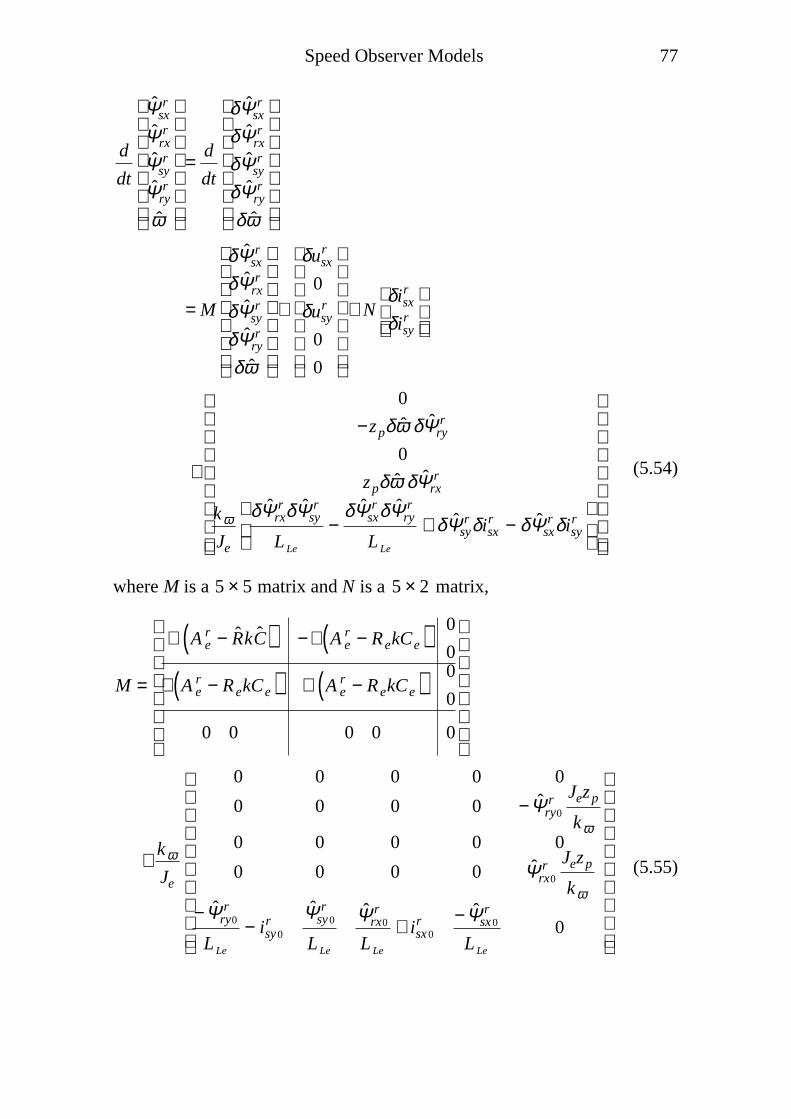
Speed Observer Models 77
d
dt
Ψsxr
Ψrxr
Ψsyr
Ψryr
ω
= d
dt
δΨsxr
δΨrxr
δΨsyr
δΨryr
δω
= M
δΨsxr
δΨrxr
δΨsyr
δΨryr
δω
+
δusxr
0
δusyr
0
0
+ Nδisx
r
δisyr
+
0
−zpδω δΨryr
0
zpδω δΨrxr
kω
Je
δΨrxr δΨsy
r
L Le
−δΨsx
r δΨryr
L Le
+ δΨsyr δisx
r − δΨsxr δisy
r
(5.54)
where M is a 5 × 5 matrix and N is a 5 × 2 matrix,
M =
ℜ A er − RkC( ) −ℑ A e
r − RekCe( ) 0
0
ℑ A er − RekCe( ) ℜ A e
r − RekCe( ) 0
0
0 0 0 0 0
+ kω
Je
0 0 0 0 0
0 0 0 0 −Ψry0r Jezp
kω0 0 0 0 0
0 0 0 0 Ψrx0r Jezp
kω−Ψry0
r
L Le
− isy0r Ψsy0
r
L Le
Ψrx0r
L Le
+ isx 0r −Ψsx 0
r
L Le
0
(5.55)

78 Speed Observer Models
N =
ℜ Rek( ) −ℑ Rek( )
ℑ Rek( ) ℜ Rek( )
kω
Je
Ψsy0r − kω
Je
Ψsx 0r
(5.56)
and A er is the observer matrix A e , but adjusted for the rotating reference
frame,
A er = A e ω0( ) − jω1 I
=−Rse
1
L Me
+ 1
L Le
− jω1
Rse
L Le
R re
L Le
−R re
L Le
+ jzpω0 − jω1
(5.57)
Ce is the same as for the stationary reference frame, defined by equation(4.7).
This observer, still non-linear, is equivalent to the observer of equations(4.21) and (5.31), but if the last term of (5.54), is neglected, we have thefollowing linear approximation,
d
dt
δΨsxr
δΨrxr
δΨsyr
δΨryr
δω
≈ M
δΨsxr
δΨrxr
δΨsyr
δΨryr
δω
+
δusxr
0
δusyr
0
0
+ Nδi sx
r
δi syr
(5.58)
This linear system can be used for studying local stability.
Poles of Linearized Speed Observer
The poles of the linearized speed observer are the eigenvalues of matrix M.If kω = 0, the poles will be the same as for the observer in a rotatingreference frame discussed in Chapter 4, plus a pole in the origin. Fig. 5.6shows how the observer poles move when kω is increased. As is seen in thefigure, a pair of the poles will move to the right half plane if the speedobserver gain is increased to much, resulting in an unstable observer.
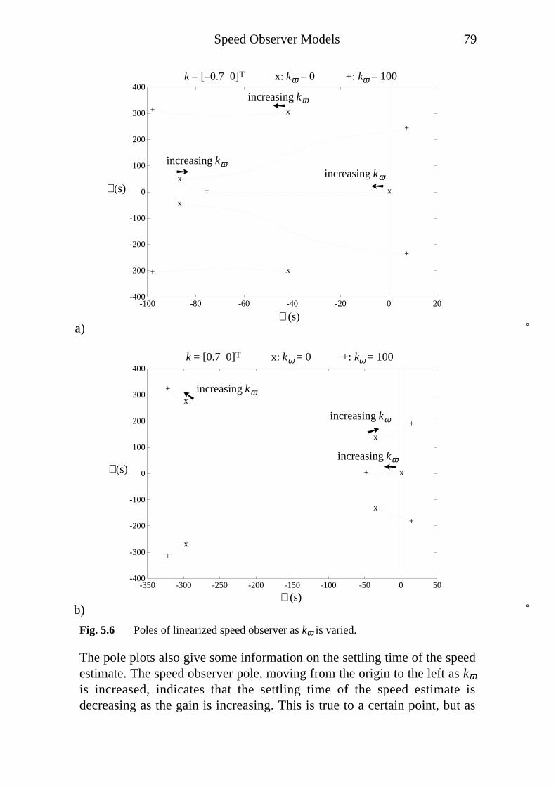
Speed Observer Models 79
a)
-400
-300
-200
-100
0
100
200
300
400
-100 -80 -60 -40 -20 0 20
x
x
x
x
x
+
+
+
+
+
Kw: 0: x, 100: +, k=0.7
ℑ (s)
ℜ (s)
increasing kω
increasing kω
increasing kω
k = [–0.7 0]T x: kω = 0 +: kω = 100
Ù
Ù
Ù
b)
-400
-300
-200
-100
0
100
200
300
400
-350 -300 -250 -200 -150 -100 -50 0 50
x
x
x
x
x
+
+
+
+
+
Kw: 0: x, 100: +, k=-0.7
ℑ (s)
ℜ (s)
increasing kω
increasing kω
increasing kω
k = [0.7 0]T x: kω = 0 +: kω = 100
Ù
Ù
Ù
Fig. 5.6 Poles of linearized speed observer as kω is varied.
The pole plots also give some information on the settling time of the speedestimate. The speed observer pole, moving from the origin to the left as kωis increased, indicates that the settling time of the speed estimate isdecreasing as the gain is increasing. This is true to a certain point, but as
80 Speed Observer Models
the flux and speed observers work hand in hand, all poles must beconsidered, and while the speed observer pole is moving to the left, a pairof the flux observer poles are moving to the right. If the flux observerbecomes too slow, the speed observer will be slower as well.
Sensitivity to Rotor Resistance
A very important property of the speed observer is seen in Fig. 5.4 b); ifthere is a ten percent error in the estimated rotor resistance, there will be aten percent error in the estimated slip.
At steady state, it is actually the ratio R r s that can be estimated if onlyvoltage and current is measured. This is independent of the structure of thespeed observer. As the rotor resistance is varying with temperature, whichin turn is varying with load, it is practically impossible to have a correctvalue of the rotor resistance at all times.
Various parameter adaptation techniques can be used to keep track of therotor resistance. One way is to measure stator winding temperature, andadjust both rotor and stator resistance according to varying temperature.The rotor temperature differs from the stator temperature, but theperformance will still be improved. Other techniques such assuperimposing ac components on the current exist (Kubota et al, 1994 andSugimoto et al, 1987).
Important Problems at Low Frequencies
Integrator drift, noise sensitivity in differentiation, error in rotor resistance,these are all problems often pointed out in articles about speed estimation(Bausch et al, 1994, Schauder, 1992 and Pohjalainen et al, 1994). However,the most important problem, lack of information in the measured signals atlow frequencies, is often neglected.
The reason that this fact so often is neglected might be that the equationsdo not reveal it at a first look. Equation (3.1) gives the stator flux, equation(5.29) gives the rotor flux, and finally equation (5.28) gives the speed. Thisscheme seems to work at all working condition, at least in theory, if theparameters are perfectly matched.
If the stator frequency f1 is zero, meaning that the stator voltage vector us isconstant, the flux vectors will be constant as well. They can be calculatedfrom equation (2.9) with the left side set to zero, as the derivatives ofconstant vectors are zero. We have

Speed Observer Models 81
0 = A Ψ + Bus (5.59)
giving
Ψ = −A −1 B us = us Rs
R r
L ML L
− j zp ω 1
L M
+ 1
L L
R r
L L
− j zp ω
R r L L
(5.60)
The current is given by equation (2.10). The flux calculated by equation(5.60) inserted into equation (2.10) gives
is = CΨ = us
Rs
(5.61)
The last two relations show why speed estimation based solely onmeasured voltage and current is impossible at zero frequency: if f1 = 0, theflux is varying with varying rotor speed, while the current is independent ofthe speed.
The problem can be illustrated in a second way. At steady state, when allvectors are rotating with constant magnitude and angular velocity, it holdsthat
dÁÁs
dt= j2π f1 ÁÁs (5.62)
Inserting (5.62) in equation (2.5) gives
ÁÁs = us − Rsis
j2π f1
(5.63)
When f1 = 0, the denominator of (5.63) becomes zero, and the stator fluxvector cannot be calculated. As the current is independent of the speedwhen f1 = 0, the measured current carries no information on the speed. Assoon as the flux vectors start to rotate, the current will be a function notonly of stator voltage us, but also a function of speed ω. The current willvary little at low frequencies, making it difficult to separate the speedinformation from noise and parameter errors. As the frequency isincreasing, the variation of the current vector is increasing, and the easier itgets to estimate the speed. Fig. 5.7 shows current vector variation atdifferent frequencies and speeds, all at rated flux, Ψs = 0.6 Vs.

82 Speed Observer Models
us
is
0 1 2 3 4 5
0
1
–1
–2
f1 = 0 Hz, ω = –5, 0 and 5 rad/s
f1 = 0.25 Hz, ω = –5, 0 and 5 rad/s
f1 = 5 Hz, ω = –5, 0 and 5 rad/s
isy [A]
isx [A]
Fig. 5.7 Current vector dependency on rotor speed ω and stator voltage frequency f1.
Note how the current vectors coincide at all speeds when f1 = 0 Hz, andthat the current and voltage vectors are parallel to each other. At 0.25 Hz,different speeds result in a small variation of the current vector, while thevariation is considerable at 5 Hz.
If the induction machine is operating at a point where the frequency isclose to zero, there is not much information for the speed observer. Fig. 5.8shows current vectors at the operating point ω = –1 rad/s and T = 1.6 Nm.The required frequency at rated flux, Ψ = 0.6 Vs, is f1 = 0.25 Hz. Withconstant amplitude and frequency of the voltage, the load torque is varied,resulting in a speed variation. At this frequency, the variation of the statorcurrent vector is negligible if ω is varying from –1.5 to –0.5 rad/s. If,however, the flux is reduced to half of its nominal value, a frequency off1 = 2.0 Hz is required to produce the same torque at ω = –1 rad/s. At thisfrequency, the variation of the stator current is increased. This variationgives more information to the speed observer.

Speed Observer Models 83
T = 1.6 Nm at ω = –1 rad/s, ω = –1.5, –1, –0.5 rad/s
–1
–0.5
0
2.5 3 3.5 4 4.5
f1 = 2.0 Hz, Ψs = 0.3 Vs
f1 = 1.0 Hz, Ψs = 0.4 Vs
f1 = 0.5 Hz, Ψs = 0.5 Vs
f1 = 0.25 Hz, Ψs = 0.6 Vs
f1 = 0.1 Hz, Ψs = 0.7 Vs
isy [A]
isx [A]
Fig. 5.8 Current vector dependency on rotor speed ω, and flux magnitude Ψs. Eachgroup of three vectors shows the current vector at the speeds ω = -1.5,ω = -1 and ω = -0.5 rad/s at the same stator voltage. The middle vector ineach group is the current vector at a load torque of 1.6 Nm.
Speed Observer Conclusions
The main problems in estimating speed based on current and voltagemeasurements is first that current and voltage carries information not onthe speed but on the relation R r s and second that this informationdisappears at f1 = 0 Hz. This means that the lower the frequency, the moredifficult it is to estimate speed. To overcome the second problem, the fluxcan be reduced at operating points with low frequencies, resulting in ahigher frequency.

6Controller Structure
This thesis is focusing on the estimation of flux and rotor speed of theinduction machine. The estimated flux and speed serve as inputs to acontroller, controlling both speed and flux. The controller is not the mainsubject here, still a controller is needed for experimental verification of theflux and speed observer properties.
No attempt has been made to look systematically for the ”best” controller.A basic stator flux oriented controller is used. However, rotor flux orientedcontrollers can also be used, as the observer estimates both stator flux androtor flux. Further discussions on controllers for induction machines arefound in the literature (Leonhard, 1985, Lorenz et al, 1994, Baader et al,1994, Takahashi et al, 1989 and Habetler et al, 1992).
Controller Overview
The complete control scheme is divided into three PI-controllers, one forthe magnitude of the stator flux vector, Ψs, one for the torque T, and onefor the speed ω. This separation can be done for example if the inductionmachine vector equations (2.3)-(2.6) are split, not in the real and imaginaryaxis directions (x and y), but in directions parallel and perpendicular to thestator flux vector. These directions will be referred to as the d- and q-directions. Index d will designate vector components parallel to the statorflux vector, and index q will designate components perpendicular to thestator flux vector. The stator flux component in the d-direction will equalthe magnitude of the stator flux vector,
Ψsd = ÁÁs = Ψs (6.1)
while its component in the q-direction is zero,
Ψsq = 0 (6.2)
The first cross product in torque equation (2.8) is actually expressing theproduct of the magnitude of the stator flux vector, and the component ofthe stator current vector at right angle to the stator flux, isq,
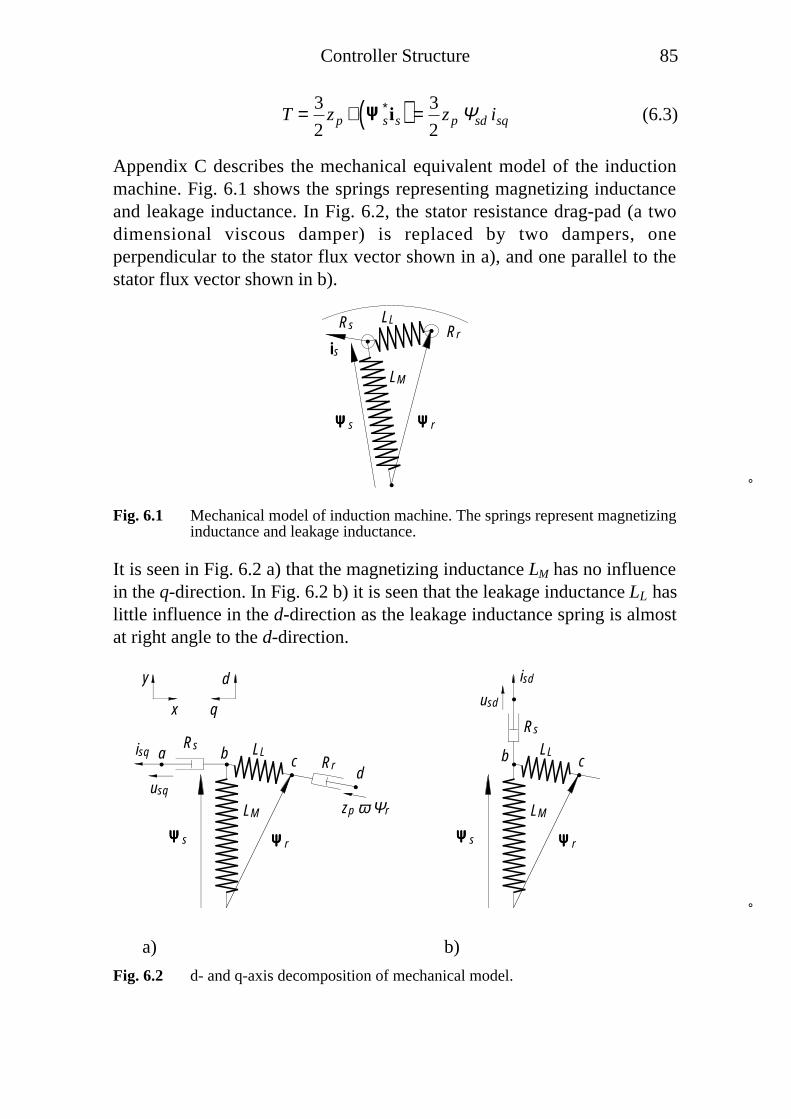
Controller Structure 85
T = 3
2zp ℑ ÁÁs
∗is( ) = 3
2zp Ψsd isq (6.3)
Appendix C describes the mechanical equivalent model of the inductionmachine. Fig. 6.1 shows the springs representing magnetizing inductanceand leakage inductance. In Fig. 6.2, the stator resistance drag-pad (a twodimensional viscous damper) is replaced by two dampers, oneperpendicular to the stator flux vector shown in a), and one parallel to thestator flux vector shown in b).
LM
is
LL
ÁÁÁÁs ÁÁÁÁr
Rs Rr
Fig. 6.1 Mechanical model of induction machine. The springs represent magnetizinginductance and leakage inductance.
It is seen in Fig. 6.2 a) that the magnetizing inductance LM has no influencein the q-direction. In Fig. 6.2 b) it is seen that the leakage inductance LL haslittle influence in the d-direction as the leakage inductance spring is almostat right angle to the d-direction.
LM
LL
ÁÁÁÁs ÁÁÁÁr
Rs
Rrisq
usq
ÁÁÁÁs ÁÁÁÁr
isd
usd
Rs
zp ω Ψr LM
LLa b cd
b c
y d
x q
a) b)
Fig. 6.2 d- and q-axis decomposition of mechanical model.

86 Controller Structure
Assuming that the leakage inductance spring and magnetizing inductancespring are at right angles to each other, the d-axis and q-axis will bedecoupled, and we have the following model shown in Fig. 6.3. Thisassumption is not completely correct. At steady state, the rotor flux vectoris perfectly perpendicular to the leakage inductance spring, while the statorflux vector is almost perpendicular.
LLRs Rrisq
usq
Ψsd
isd
usd
Rs
zp ω Ψr
a b bc d
LM
a) b)
Fig. 6.3 approximate dq-decomposition. a) q-axis model b) d-axis model.
The purpose of one controller, the flux controller, is to keep the magnitudeof the stator flux constant. With constant stator flux magnitude, the torquecan be controlled by controlling isq, which is done by the torque controller.Finally, the speed controller gives the torque reference, as indicated in Fig.6.4. There are methods referred to as direct torque control (Takahashi et al,1989, Baader et al, 1992 and Pohjalainen et al, 1994) where the flux andtorque controllers are not separated, with reported better dynamicperformance than the controller structure described here.
fluxcontroller
torquecontroller
speedcontroller
coordinatetransformation
isq
isqref
Ψsdˆ
ω
ωref
usd
usq
usx
usy
Ψsdref
Fig. 6.4 Block diagram of controller structure. Estimated flux and speed are used ascontroller inputs.

Controller Structure 87
Note that the estimated flux, and not the actual flux is controlled, as theactual flux usually cannot be measured.
Flux Controller
The flux controller is approximately controlling the system in Fig. 6.3 b),described by
dΨsd
dt= usd − R s
L M
Ψsd (6.4)
or with the Laplace transform
sÁÁsd = usd − R s
L M
ÁÁsd (6.5)
where ÁÁsd is the Laplace transform of Ψsd , and u sd is the Laplacetransform of usd. In the following sections of this chapter, bold typefacewill distinguish Laplace transforms from the corresponding time function.
A PI-controller is described by
y = k p e + 1
Ti
e dt∫
(6.6)
where kp is the proportional gain, Ti is the integration time, e is the error ofthe controlled quantity, and y is the controller output. Let usd be the outputof the controller, and let Ψsdref − Ψsd be the error. With these substitutionstogether with the Laplace transform, equation (6.6) can be written
usd = k p 1 + 1
sTi
ÁÁsdref − ÁÁsd( ) (6.7)
Combining (6.5) and (6.7) gives the transfer function H(s) of the closedloop system,
ÁÁsd = H s( )ÁÁsdref = k p
s + 1
Ti
s2 + sR s
L M
+ k p
+
k p
Ti
ÁÁsdref (6.8)
with the characteristic polynomial

88 Controller Structure
P s( ) = s2 + sRs
L M
+ k p
+
k p
Ti
(6.9)
A general polynomial of the second order can be written
s2 + 2ζ Ω s + Ω2 (6.10)
where Ω is the natural frequency and ζ is the relative damping. The naturalfrequency of the flux controller system is
Ω = k p Ti (6.11)
and the relative damping is
ζ = Rs
L M
+ k p
Ti
4k p
(6.12)
Torque Controller
The torque controller structure is similar to the flux controller structurewith one exception; the equation describing Fig. 6.3 a) contains one termdependent on the rotor speed ω and the magnitude of the rotor flux Ψr
(assumed to be constant to avoid non-linearities),
sL L isq = usq − Rs + R r( )isq − zp ∑∑ Ψr (6.13)
This term can be dealt with by adding a feed forward term yff to the PI-controller in equation (6.6),
y = k p e + 1
Ti
e dt∫
+ yff (6.14)
The output of the torque controller is usq and the error signal is isqref − isq .The feed forward term should be equal to the rotor speed dependent term,zp ω Ψr. The Laplace transform of the torque controller is described by
usq = k p 1 + 1
sTi
isqref − isq( ) + zp ∑∑ Ψr (6.15)
If the rotor speed ω and rotor flux magnitude Ψr are estimated instead ofmeasured, the feed forward term in (6.15) should be replaced by zp ∑∑ Ψr.Equation (6.13) and (6.15) give the closed loop transfer function,
Controller Structure 89
isq = H s( )isqref =k p
L L
s + 1
Ti
s2 + sRs + R r + k p
L L
+k p
TiL L
isqref (6.16)
The natural frequency is
Ω =k p
TiL L
(6.17)
and the relative damping is
ζ = Rs + R r + k p( ) Ti
4k pL L
(6.18)
Speed Controller
The system regulated by the speed controller is described by equation (2.7),with the Laplace transform
s J∑∑ = T − Tload (6.19)
Again, a PI-controller will be used, where Tref is the output and ωref − ω isthe error. The Laplace transform of the controller can be written
Tref = k p 1 + 1
sTi
∑∑ ref − ∑∑( ) (6.20)
Assuming that the torque controller is significantly faster than the speedcontroller, Tref and T can be considered equal in the speed controller timescale. With
T = Tref (6.21)
equations (6.19) and (6.20) can be combined into
∑∑ =k p
J
s + 1
Ti
s2 + sk p
J+
k p
JTi
∑∑ ref − 1
J
s
s2 + sk p
J+
k p
JTi
Tload (6.22)
with the natural frequency

90 Controller Structure
Ω =k p
JTi
(6.23)
and relative damping
ζ =k p Ti
4 J(6.24)
According to Fig. 6.4, the output of the speed controller should be areference for the current isq and not the torque reference Tref as in equation(6.20). Equation (6.3) gives the relation between isq and the torque T. Thedesired current reference is given by
isqref = 2
3zp Ψsdref
Tref (6.25)
If the speed is estimated instead of measured, ∑∑ should be replaced by ∑∑in equations (6.19), (6.20) and (6.22).
Further connections between the controller, the observer, the motor andpower electronics are discussed in Chapter 7.

7Implementation
The flux observer, speed observer, and controller described in earlierchapters have been tested in a laboratory set-up described in this chapter.
General Configuration of Laboratory Set-up
The set-up is shown in Fig. 7.1 and Fig. 7.3. On top of the instrument rackin Fig. 7.1, an induction machine with an incremental encoder is placed,shown in detail in Fig. 7.2. The incremental encoder is used only forcomparison of the estimated and actual speed of the induction machine.The ratings and parameters of the induction machine are found inAppendix D.
a) b) Fig. 7.1 Instrument rack with controlled induction machine at the top and braking
DC machine at the bottom. a) side view b) top view

92 Implementation
The 0.75 kW machine used in the set-up is in no way representative to allinduction machines. The p.u. stator resistance is much higher for such asmall machine than for a larger one. However, as a large stator resistancemakes flux estimation and speed estimation more difficult at lowfrequencies, the chosen machine represents a ”near worst case”.
a)
b)
Fig. 7.2 a) induction machine with incremental encoder b) permanent magnet DCmachine providing load torque for the induction machine.

Implementation 93
A DC machine with torque control providing load torque for the inductionmachine is placed at the bottom of the rack.
The induction machine and DC machine are connected via a belt drive. AnIGBT inverter bridge, current and voltage sensors and computer interfacehardware are placed between the two machines. The same set-up has beenused for position control experiments (Samuelsson, 1994).
a)
b)
Fig. 7.3 a) Macintosh computer holding the DSP board. b) DSP board.

94 Implementation
The rack is connected to computer hardware consisting of a digital signalprocessor (DSP) board and a multi purpose I/O board, both from NationalInstruments, placed in a Macintosh IIci computer, shown in Fig. 7.3. TheDSP, a TMS320C30 from Texas Instruments is of floating point type, andwas chosen because of its ease of use in an experimental environment. Inan industrial application, the floating point DSP would be replaced by aless expensive fixed point DSP.
Fig. 7.4 LabVIEW control panel.
The observer and controller calculations are performed by the DSP, while agraphical user interface is running on the Macintosh. The user interface isrealized as a virtual instrument, developed with the LabVIEW softwarefrom National Instruments. The LabVIEW control panel is shown in Fig.7.4. The user can select inverter (inv) or controller (ctrl) mode. In invertermode, the induction machine is running in open loop as if it was connectedto a standard open loop frequency inverter with features like RI-compensation, ramp times, and set-point frequency (Peterson, 1996). With

Implementation 95
the observer running at the same time, the estimated and measured speedcan be compared, and the observer can be tuned. In controller mode, theclosed loop controller described in Chapter 6 is controlling the inductionmachine based on the estimated flux and speed. The measured speedinstead of estimated speed can also be chosen as controller input.
Excluding the machines, the set-up consists of four logical blocks shown inFig. 7.5: the control panel, the observer, the controller, and a voltage sourceinverter.
IM DCobserver controllervoltage source
inverter
controlled induction machine
braking DC machineus, is
LabVIEWcontrol panel
observer gain
controller gain and speed reference
Fig. 7.5 Connections between control panel, observer, controller and inverter.
Voltage Source Inverter Implementation
Diagrams of the voltage source inverter are shown in Fig. 7.6.
IMDSP timer x 3IGBT
inverterbridge
a)
dead time logicand gate driver
+dc linkvoltage
–
switch command signal from timer
IMb)
idc
Fig. 7.6 Voltage source inverter. a) block diagram of the inverter b) IGBT inverter
bridge. Each leg is controlled by a timer.

96 Implementation
The inverter consists of a pulse width modulator and an IGBT inverterbridge supplied by a diode rectifier which is not shown in the figure. Thepulse width modulator is realized by three timer circuits together with theDSP. For each sample interval, the DSP loads the timers with appropriateswitch patterns for the desired voltage vector, emulating the pulse widthmodulation method where a triangular wave form is compared with acontrol voltage (Mohan et al, 1989). Each timer controls one leg of theinverter bridge.
Observer Implementation
The observer can be implemented in several ways. If the DC link voltage ofthe voltage source inverter is measured, and the states of the switches in theinverter are known, the stator voltage vector us can be calculated. However,this method requires the switches to be ideal if an accurate value should beobtained. Normally there is a delay between the time when one transistor isturned off and the other transistor is turned on in one inverter leg. Thisdelay is usually called the deadtime, and makes the calculated outputvoltage differ from the true voltage. Resistive voltage drop in thetransistors contribute as well to the error in the calculated voltage. To avoidproblems due to deadtime and voltage drop, the output voltage of all threephases can be measured. This method gives a new problem; as the outputvoltage is a switched voltage, it must be filtered before it is A/D-convertedand fed to the DSP, introducing time delays in the measured voltage.
These problems are solved if analogue integrators are used instead. Fig. 7.7shows how the output voltage us of the inverter is fed to an analogueintegrator. The output of the integrator is then A/D-converted and fed to theDSP. If Fig. 7.7 is compared with Fig. 4.1, it is seen that only the statorflux integration and one subtraction need to be performed outside the DSP,while all the other observer calculations can be done by the DSP. The inputvoltage to this combined analogue and digital observer is identical to thevoltage seen by the induction machine, and no compensation for deadtimeand voltage drop is needed.
The rotor flux integration in equation (4.14) and the speed integration inequation (5.31) are approximated by first order Euler approximations.Instead of Euler approximations of the continuous time system, a discrete-time representation of the system can be calculated (Åström et al, 1984).With periodic sampling time h, the discrete-time representation of thegeneral system in (3.10) is given by

Implementation 97
x kh + h( ) = Φx kh( ) + Γu kh( ) (7.1)
where
Φ = eAh (7.2)
and
Γ = eAsdsB0
h∫ (7.3)
This is straightforward for a time-invariant system, but as the matrix A forthe induction motor is varying with ω, the discrete-time representationmust be updated for each sample. Using (7.2) and (7.3) for an on-lineupdate is too time consuming. However, an approximation of (7.2) and(7.3), presented by Böcker et al (1991) makes on-line calculation possible.Still, the Euler approximation was chosen here due to its simplicity. Therehave been reports on disastrous performance by flux observers using theEuler approximation (Verghese et al, 1988), but it must be noted that allintegrators were approximated in those examples. In the set-up describedhere, the analogue integrators shown in Fig. 7.7 are working continuously,and need not be approximated at all.
1/LMe
is
Rse+–
ks 1+ks+–
+–
ˆus ÁÁÁÁs
is
D/A
Digital Signal ProcessorAnalogue Integratorand A/D-D/A converters
A/D
A/D
+– ∫
Fig. 7.7 Observer implementation combining analogue and digital integrators.
Controller Implementation
All controller calculations are performed by the DSP, again using firstorder Euler approximations for the integral parts. The output of thecontroller is the desired stator voltage vector. Based on this vector, the DSP

98 Implementation
calculates an appropriate switch pattern and loads the timers as describedabove.
DSP programming
The DSP is programmed using the high level C language (Peterson, 1996).To further facilitate high level programming, a real time kernel (Carlsson,1993) has been developed. Both the controller and the observer run with asample period of 500 µs. The choice of sample period in this configurationis limited by the relatively slow A/D-converters being used. Thecalculations can be done in a fraction of this time. As this thesis is focusingon the low frequency region, where flux vectors and other quantities areslowly varying, the sample period of 500 µs is acceptable, even though ashorter sampling period would be preferred.

8Measurements
To evaluate the performance of the system, a series of measurements hasbeen accomplished. The measurements can be divided into three groups:
• a step change of the load torque at constant speed reference;
• a step change of the speed reference at constant load torque;
• a slow ramp of the speed reference at constant load torque.
As the most critical problems arise at low speed and low frequency, allmeasurements are done in a speed range of 0–20% of rated speed.
Step Change of Load Torque
Fig. 8.1 shows two cases of a change in load torque at constant speedreference ωref = 0. The upper diagram shows a step change in the loadtorque at an observer gain k = −0.7 0[ ]T while the gain is k = 2 0[ ]T inthe lower diagram. It can be seen that the steady state error is smaller in theupper diagram. In Fig. 5.4 and Fig. 5.5 it was also seen thatk = −0.7 0[ ]T resulted in a small steady state error. It is seen in the upperdiagram that there is a slow beat in the speed signal when the load torque iszero. At zero speed and zero torque, the frequency f1 of the stator voltageshould be zero. At zero frequency, there is not enough information for theobserver to keep the speed perfectly at zero, as was described in Chapter 5,in the section Important Problems at Low Frequencies.
In Fig. 8.2 and Fig. 8.3, the speed reference is 5 rad/s (3.5% of rated speed)and 10 rad/s (7% of rated speed) respectively. In both cases, the statorfrequency will differ from zero, and the beat that occurred at zerofrequency is no longer present. Again, the steady state error is smaller atk = −0.7 0[ ]T .

100 Measurements
a)
-10
-5
0
5
10
15
20
25
0 1 2 3 4 5 6
#1 do160152 k=[0.7; 0] omegaref=-1.118e-06
t
omeg
a
rated load torque6 7444 8444
no load torque6 7444 8444
no load torque6 7444 8444
t [s]
ω [rad/s]
ωref = 0 rad/s, k = [–0.7 0]T
b)
-10
-5
0
5
10
15
20
25
0 1 2 3 4 5 6
#2 do160715 k=[-2; 0] omegaref=-1.118e-06
t
omeg
a
t [s]
ω [rad/s]
ωref = 0 rad/s, k = [2 0]T
rated load torque6 7444 8444
no load torque6 7444 8444
no load torque6 7444 8444
Fig. 8.1 Step change of load torque at constant speed reference ωref = 0. a)
k = −0.7 0[ ]T b) k = 2 0[ ]T

Measurements 101
a)
-10
-5
0
5
10
15
20
25
0 0.5 1 1.5 2 2.5 3
#3 do155250 k=[0.7; 0] omegaref=5
t
omeg
a
t [s]
ω [rad/s]
ωref = 5 rad/s, k = [–0.7 0]T
rated load torque6 7444 8444
no load torque6 7444 8444
no load torque6 7444 8444
b)
-10
-5
0
5
10
15
20
25
0 0.5 1 1.5 2 2.5 3
#4 do160438 k=[-2; 0] omegaref=5
t
omeg
a
t [s]
ω [rad/s]
ωref = 5 rad/s, k = [2 0]T
rated load torque6 7444 8444
no load torque6 7444 8444
no load torque6 7444 8444
Fig. 8.2 Step change of load torque at constant speed reference ωref = 5 rad/s (3.5%
of rated speed). a) k = −0.7 0[ ]T b) k = 2 0[ ]T

102 Measurements
a)
-10
-5
0
5
10
15
20
25
0 0.5 1 1.5 2 2.5 3
#5 do160000 k=[0.7; 0] omegaref=10
t
omeg
a
t [s]
ω [rad/s]
ωref = 10 rad/s, k = [–0.7 0]T
rated load torque6 7444 8444
no load torque6 7444 8444
no load torque6 7444 8444
b)
-10
-5
0
5
10
15
20
25
0 0.5 1 1.5 2 2.5 3
#6 do164454 k=[-2; 0] omegaref=10
t
omeg
a
t [s]
ω [rad/s]
ωref = 10 rad/s, k = [2 0]T
rated load torque6 7444 8444
no load torque6 7444 8444
no load torque6 7444 8444
Fig. 8.3 Step change of load torque at constant speed reference ωref = 10 rad/s (7%
of rated speed). a) k = −0.7 0[ ]T b) k = 2 0[ ]T

Measurements 103
Step Change of Speed Reference
In Fig. 8.4 and Fig. 8.5, the load torque is equal to rated torque in the upperdiagrams and equal to zero in the lower diagrams.
a)
-20
-15
-10
-5
0
5
10
15
20
0 0.2 0.4 0.6 0.8 1 1.2
do1 951127 Kw=0.5 k=[0.7; 0] rated load torque
t
omeg
a (s
olid
) om
egar
ef (
dash
ed)
6 7444 8444 6 7444 84446 7444 8444
generator, s < 0,f1 ≈ 1 Hz
t [s]
ω (
solid
)
ωre
f (da
shed
) [
rad/
s]
rated load torque, k = [–0.7 0]T
motor, s > 0,f1 ≈ 5 Hz
generator, s < 0,f1 ≈ 1 Hz
b)
-20
-15
-10
-5
0
5
10
15
20
0 0.2 0.4 0.6 0.8 1 1.2
do2 951127 Kw=0.5 k=[0.7; 0] zero load torque
t
omeg
a (s
olid
) om
egar
ef (
dash
ed)
6 7444 8444 6 7444 84446 7444 8444s ≈ 0, f1 ≈ 3.4 Hz
t [s]
ω (
solid
)
ωre
f (da
shed
) [
rad/
s]
zero load torque, k = [–0.7 0]T
s ≈ 0, f1 ≈ 3.4 Hz s ≈ 0, f1 ≈ 3.4 Hz
Fig. 8.4 Step change of speed reference from –10 to +10 rad/s (7% of rated speed).a) rated load b) zero load

104 Measurements
The speed reference is changed from –10 to +10 rad/s and back to –10rad/s in Fig. 8.4. At negative speed and positive torque, the slip is negative,and the induction machine is running as a generator. As the diode rectifiersupplying the inverter bridge in Fig. 7.6 does not accept a negative currentidc, power cannot be fed from the induction machine to the supply.However, the generated power at ω = −10 rad / s is less than the internallosses in the induction machine. It is seen that the error in the speed islarger at ω = −10 rad / s than at ω = +10 rad / s . This is no surprise as thefrequency of the stator voltage is lower in generator case (about 1 Hz) thanin the motor case (about 5 Hz), and the lower the frequency, the harder it isto estimate the speed. In the lower diagram of Fig. 8.4, the load is zero andthe machine is running approximately with zero slip in both directions,giving identical performance at positive and negative speed. The overshootin the speed is a combination of observer and controller properties. Achange of the gain of the controller can reduce the overshoot, but as thespeed controller input is the estimated speed and not the actual speed, aperfectly tuned controller would not have perfect performance due toobserver dynamics.
Fig. 8.5 shows a step in the speed reference from 0 rad/s to +10 rad/s andback to 0 rad/s, with rated load torque in the upper diagram and zero loadtorque in the lower. When the speed reference is going from 10 to 0 rad/s atrated load, it takes some time before the speed stabilizes. The reason is thatthe stator voltage frequency f1 must fall from about 5 Hz down to 1 Hz.There is an undershoot in the frequency, almost reaching 0 Hz. When thefrequency temporarily is close to 0 Hz, there will be an error in the speed.This is further accentuated in the next section, when the speed reference isslowly changed. Comparing the upper diagrams of Fig. 8.4 and Fig. 8.5shows that f1 = 0 at rated torque at ω = 0 and ω = −10 rad / s . However, thestator voltage vector is rotating in different directions in the two cases.
Both diagrams in Fig. 8.6 show a step change of the speed reference at zeroload torque, but up to 25 rad/s instead of 10 rad/s as before. The response iscomparable to that of Fig. 8.4 and Fig. 8.5.
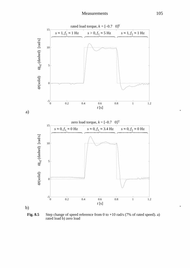
Measurements 105
a)
-5
0
5
10
15
0 0.2 0.4 0.6 0.8 1 1.2
do3 951127 Kw=0.5 k=[0.7; 0] rated load torque
t
omeg
a (s
olid
) om
egar
ef (
dash
ed)
6 7444 8444 6 7444 84446 7444 8444s ≈ 1, f1 ≈ 1 Hz
t [s]
ω (
solid
)
ωre
f (da
shed
) [
rad/
s]
rated load torque, k = [–0.7 0]T
s > 0, f1 ≈ 5 Hz s ≈ 1, f1 ≈ 1 Hz
b)
-5
0
5
10
15
0 0.2 0.4 0.6 0.8 1 1.2
do4 951127 Kw=0.5 k=[0.7; 0] zero load torque
t
omeg
a (s
olid
) om
egar
ef (
dash
ed)
6 7444 8444 6 7444 84446 7444 8444s ≈ 0, f1 ≈ 0 Hz
t [s]
ω (
solid
)
ωre
f (da
shed
) [
rad/
s]
zero load torque, k = [–0.7 0]T
s ≈ 0, f1 ≈ 3.4 Hz s ≈ 0, f1 ≈ 0 Hz
Fig. 8.5 Step change of speed reference from 0 to +10 rad/s (7% of rated speed). a)rated load b) zero load

106 Measurements
a)
-10
-5
0
5
10
15
20
25
30
35
40
0 0.2 0.4 0.6 0.8 1 1.2
do5 951127 Kw=0.5 k=[0.7; 0] zero load torque
t
omeg
a (s
olid
) om
egar
ef (
dash
ed)
6 7444 8444 6 7444 84446 7444 8444s ≈ 0, f1 ≈ 0 Hz
t [s]
ω (
solid
)
ωre
f (da
shed
) [
rad/
s]
zero load torque, k = [–0.7 0]T
s ≈ 0, f1 ≈ 8 Hz s ≈ 0, f1 ≈ 0 Hz
b)
-50
-40
-30
-20
-10
0
10
20
30
40
50
0 0.2 0.4 0.6 0.8 1 1.2
do6 951127 Kw=0.5 k=[0.7; 0] zero load torque
t
omeg
a (s
olid
) om
egar
ef (
dash
ed)
6 7444 8444 6 7444 84446 7444 8444s ≈ 0, f1 ≈ 8 Hz
t [s]
ω (
solid
)
ωre
f (da
shed
) [
rad/
s]
zero load torque, k = [–0.7 0]T
s ≈ 0, f1 ≈ 8 Hz s ≈ 0, f1 ≈ 8 Hz
Fig. 8.6 Step change of speed reference at zero load a) 0 to 25 rad/s (17% of ratedspeed). b) –25 to 25 rad/s.
Slow Ramp of Speed Reference
Fig. 8.7 shows a positive and a negative ramp of the speed reference,between –10 rad/s and +10 rad/s.
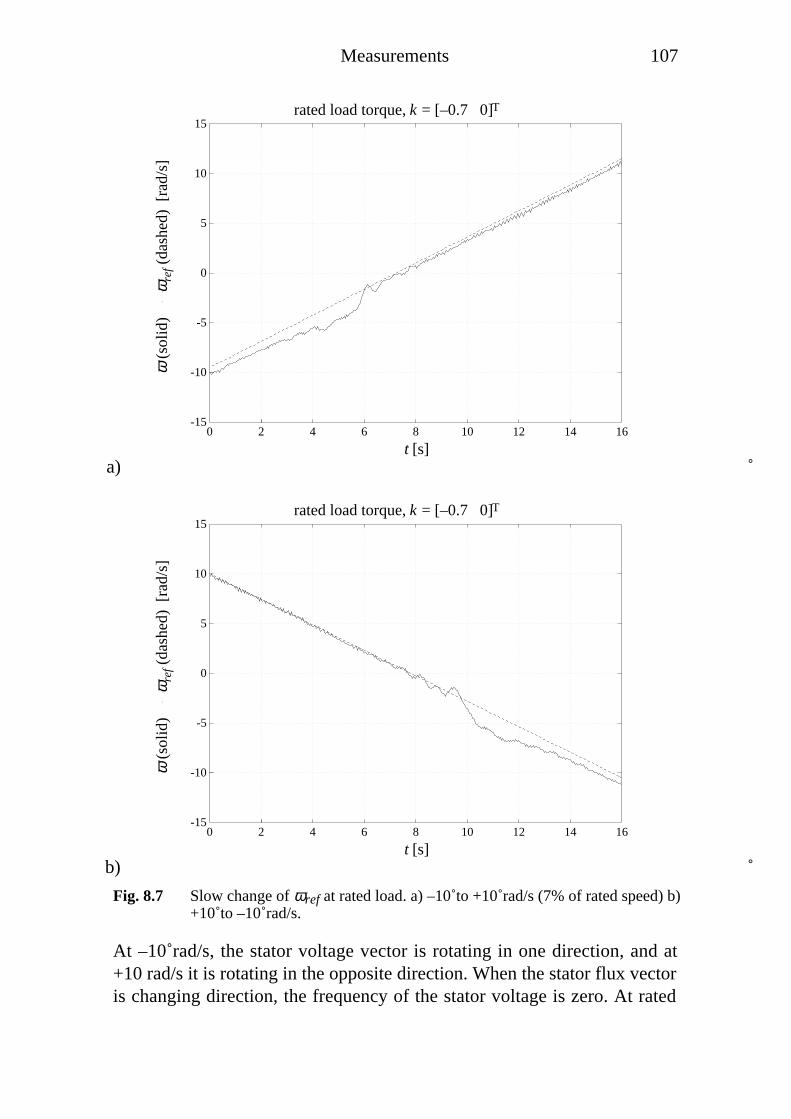
Measurements 107
a)
-15
-10
-5
0
5
10
15
0 2 4 6 8 10 12 14 16
do7 951127 Kw=0.5 k=[0.7; 0] rated load torque
t
omeg
a (s
olid
) om
egar
ef (
dash
ed)
t [s]
ω (
solid
)
ωre
f (da
shed
) [
rad/
s]
rated load torque, k = [–0.7 0]T
b)
-15
-10
-5
0
5
10
15
0 2 4 6 8 10 12 14 16
do8 951127 Kw=0.5 k=[0.7; 0] rated load torque
t
omeg
a (s
olid
) om
egar
ef (
dash
ed)
t [s]
ω (
solid
)
ωre
f (da
shed
) [
rad/
s]
rated load torque, k = [–0.7 0]T
Fig. 8.7 Slow change of ωref at rated load. a) –10 to +10 rad/s (7% of rated speed) b)+10 to –10 rad/s.
At –10 rad/s, the stator voltage vector is rotating in one direction, and at+10 rad/s it is rotating in the opposite direction. When the stator flux vectoris changing direction, the frequency of the stator voltage is zero. At rated
108 Measurements
load, this occurs at about ω = −3rad / s, and it is clearly seen that there isan error in the estimated speed in a region close to ω = −3rad / s. Thiscould be expected from the results in section Important Problems at LowFrequencies of Chapter 5.
In conclusion, the results regarding parameter sensitivity at differentobserver gains, and the problems at low frequency operation, as well as thegeneral behaviour of the observer discussed in earlier chapters, have beenexperimentally verified.

9Conclusion
With mechanical analogies, and simplified examples, many of the hiddenmysteries of speed and flux observers have been clarified. With theknowledge acquired from these examples, it has been possible to obtain anobserver which does not suffer from integrator drift and other problemsreported elsewhere.
This observer can be used in a sensorless vector control drive system,filling the gap between open loop frequency inverter systems and vectorcontrol systems using speed measurement. The dynamic performance ofthe sensorless system with speed estimation is superior to an open loopfrequency inverter system. Even though it will never show the sameaccuracy near zero speed as a system with a speed sensor on the motorshaft, the sensorless system can increase the performance in applicationswhere open loop inverters are used today, and it can be used in manyapplications which otherwise would require a speed sensor.
The sensorless system uses the same inverter bridge configuration as in anopen loop frequency inverter, with little additional hardware, and anystandard induction motor can be used. The main difference is that observerand controller calculations are performed by a digital signal processor. Asthe cost of a suitable fixed point DSP is less than $10 (1995), the overallcost of the sensorless system is equal to the cost of an open loop invertersystem.
Future Topics
The remaining problems are two; the lack of information at zero frequency,and the error in estimated speed due to errors in the rotor resistanceparameter of the observer.
It is believed that both problems can be reduced by superimposingperturbation signals on the supply voltage. A perturbation in the d-axis,parallel to the magnetizing flux, would not directly affect the producedtorque of the motor, but would give additional information to the observer.This would only require additional calculations, without any modificationsof motors or inverters.

110

References
1) Baader, U., M. Depenbrock, G. Gierse (1992) ”Direct Self Control(DSC) of Inverter-Fed Induction Machine: A Basis for SpeedControl Without Speed Measurement”, IEEE Transactions onIndustry Applications, vol. 28, no. 3, May/June 1992, pp. 581-588.
2) Bausch H., K. Kanelis, B. Lange, W. Zeng (1994) ”Torque Controlof Synchronous and Asynchronous Drives Without MechanicalSensors”, Proc. ICEM ’94, Paris, France, pp. 324-328.
3) Beguenane, R., C. Ghyselen, H. Schoorens (1994), ”A ProposedInduction Motor Speed Sensor Without Contact from SlotsHarmonics: Application to Rotoric Time Constant Identification”,Proc. 1994 IEE Conf., London, UK, pp. 90-95.
4) Böcker, J., J. Janning (1991), ”Discrete-Time Flux Observer forPWM Inverter Fed Induction Motors, Proc. EPE ’91, Firenze, Italy,pp. 171-176.
5) Carlsson, A. (1993), Liten, snabb realtidskärna i C (in Swedish),Department of Automatic Control, LTH, Lund, Sweden
6) Glad, T., L. Ljung (1981), R e g l e r t e k n i k (in Swedish),Studentlitteratur, Lund, Sweden
7) Habetler, T. G., F. Profumo, M. Pastorelli, L. M. Tolbert (1992),”Direct Torque Control of Induction Machines Using Space VectorModulation”, IEEE Transactions on Industry Applications, vol. 28,no. 5, September/October 1992, pp. 1045-1053.
8) Haemmerli, B. M. (1986), ”Rotor Speed Detection for InductionMachines Utilising Rotor Slots Harmonics”, Proc. ICEM ’86, pp.352-354.
9) Henneberger, G., B.-J. Brunsbach, Th. Klepsch (1991), ”Field-Oriented Control of Synchronous and Asynchronous Drives withoutMechanical Sensors Using a Kalman Filter”, Proc. EPE ’91, Firenze,Italy, pp. 664-669.
10) Hori, Y., V. Cotter, Y. Kaya (1987), ”A Novel Induction MachineFlux Observer and its Application to a High Performance AC Drive

112 References
System”, Proc. IFAC 10th Triennial World Congress, Munich, FRG,pp. 363-368.
11) Hurst, K. D., T. G. Habetler, G. Griva, F. Profumo (1994), ”SpeedSensorless Field-Oriented Control of Induction Machines UsingCurrent Harmonic Spectral Estimation”, Proc. IAS ’94 29th AnnualMeeting, Denver Colorado, pp. 601-607.
12) Jansen, P. L., R. D. Lorenz (1994a), ”Transducerless Position andVelocity Estimation in Induction and Salient AC Machines”, Proc.IAS ’94 29th Annual Meeting, Denver Colorado, pp. 488-495.
13) Jansen, P. L., R. D. Lorenz (1994b), ”A Physically InsightfulApproach to the Design and Accuracy Assessment of Flux Observersfor Field Oriented Induction Machine Drives”, IEEE Transactions onIndustry Applications, vol. 30, no. 1, January/February 1994, pp.101-110.
14) Jansen, P. L., R. D. Lorenz (1993) ”Accuracy Limitations ofVelocity and Flux Estimation in Direct Field Oriented InductionMachines”, Proc. EPE ’93, Brighton, UK, pp. 312-318.
15) Jönsson, R. (1991), Natural Field Orientation, Patent ApplicationPCT/SE91/00086.
16) Kim, Y.-R., S.-K. Sul, M.-H. Park (1994), ”Speed Sensorless VectorControl of Induction Motor using Extended Kalman Filter”, IEEETransactions on Industry Applications , vol. 30, no. 5,September/October 1994, pp. 1225-1233.
17) Kovács, P. K. (1984), Transient Phenomena in Electrical Machines,Elsevier, Amsterdam.
18) Krzeminski, Z. (1991) ”Speed and Rotor Resistance Estimation inObserver System of Induction Motor”, Proc. EPE ’91, Firenze, Italy,pp. 538-542.
19) Kubota, H., K. Matsuse (1994), ”Speed Sensorless Field-OrientedControl of Induction Motor with Rotor Resistance Adaption”, IEEETransactions on Industry Applications , vol. 30, no. 5,September/October 1994, pp. 1219-1224.
20) Leonhard, W. (1985), Control of Electrical Drives, Springer, Berlin.
21) Lorenz, R. D., T. A. Lipo, D. W. Novotny (1994), Motion Controlwith Induction Motors, University of Wisconsin, Madison, WI.
22) Luenberger, D. G. (1979), Introduction to Dynamic Systems, JohnWiley & Sons, USA.

References 113
23) Menander, F., J. Silvander (1991), Flödesobserverare förasynkronmotor (in Swedish), Department of Automatic Control,LTH, Lund, Sweden.
24) Mohan, N., T. M. Undeland, W. P. Robbins (1989), PowerElectronics: Converters, Applications and Design, John Wiley &Sons, USA.
25) Peterson (1991), Oscillations in Inverter Fed Induction MotorDrives, IEA/LTH, Lund, Sweden.
26) Peterson (1996), DSP Implementation of Induction Machine SpeedObserver, IEA/LTH, Lund, Sweden
27) Pohjalainen. P., P. Tiitinen, J. Lalu (1994), ”The Next GenerationMotor Control Method - Direct Torque Control, DTC”, EPE ChapterSymposium, Electric Drive Design and Applications, Lausanne,Switzerland, pp. 115-120.
28) Samuelsson, O. (1994), Point-to-point Position Control using SimpleMechanical Sensors, IEA/LTH, Lund, Sweden.
29) Schauder, C. (1992) ”Adaptive Speed Identification for VectorControl of Induction Motors without Rotational Transducers”, IEEETransactions on Industry Applications , vol. 28, no. 5,September/October 1992, pp. 1054-1061.
30) Schroedl, M.(1992), ”Sensorless Control of Induction Motors at LowSpeed and Stand Still”, Proc. ICEM ’92, Manchester, UK, pp. 863-867.
31) Slemon, G., A. Straughen (1980), Electric Machines, Addison-Wesley, Reading, Mass.
32) Sugimoto, H., S. Tamai (1987), ”Secondary Resistance Identificationof an Induction Motor Applied Model Reference Adaptive Systemand its Characteristics”, IEEE Transactions on Industry Applications,vol. IA-23, no. 2, March/April 1987, pp. 296-303.
33) Tajima, H., Y. Hori (1993), ”Speed Sensorless Field-OrientationControl of the Induction Machine”, IEEE Transactions on IndustryApplications, vol. 29, no. 1, January/February 1993, pp. 175-180.
34) Takahashi. I., Y. Ohmori (1989), ”High-Performance Direct TorqueControl of an Induction Motor”, IEEE Transactions on IndustryApplications, vol. 25, no. 2, March/April 1989, pp. 257-264.
35) Tamai, S., H. Sugimoto, M. Yano (1987), ”Speed Sensor-less VectorControl of Induction Motor with Model Reference Adaptive

114 References
System”, Proc. IEEE Industry Applications Society Annual Meeting1987, pp. 189-195.
36) Török, V., J. Valis (1985), Elektroniska drivsystem (in Swedish),Tutext, Stockholm.
37) Umeno, T., Y. Hori, H. Suzuki (1990), ”Design of the Flux-Observer-Based Vector Control System of Induction MachinesTaking into Consideration Robust Stability”, Electrical Engineeringin Japan, vol. 110, no. 6, pp. 53-65.
38) Vélez-Reyes, M., G. C. Verghese (1995), ”Subset Selection inIdentification, and Application to Speed and Parameter Estimationfor Induction Machines”, Proc. 4th IEEE Conf. on ControlApplications, Albany, NY, pp. 991-997.
39) Veltman, A. (1994), The Fish Method, Delft University Press, Delft,The Netherlands.
40) Verghese, G. C., S. R. Sanders (1988), ”Observers for FluxEstimation in Induction Machines” IEEE Transactions on IndustrialElectronics, vol. 35, no. 1, February 1988, pp. 85-94.
41) von Westerholt, E., M. Pietrzak-David, B. de Fornel (1992a),”Extended State Estimation of Nonlinear Modeled InductionMachines”, Proc. PESC ’92, Toledo, Spain, pp. 271-278.
42) von Westerholt, E., M. Pietrzak-David, B. de Fornel (1992b),”Extended Kalman Filter based Control of Low-Power InductionMotor Drives for Robotic Applications”, Proc. ICEM ’92,Manchester, UK, pp. 843-847.
43) Yang, G., T.-H. Chin (1993), ”Adaptive-Speed IdentificationScheme for a Vector Controlled Speed Sensorless Inverter-InductionMotor Drive”, IEEE Transactions on Industry Applications, vol. 29,no. 4, July/August 1993, pp. 820-825.
44) Zai, L.-C., C. L. DeMarco, T. A. Lipo (1992), ”An Extended KalmanFilter Approach to Rotor Time Constant Measurement in PWMInduction Motor Drives”, IEEE Transactions on IndustryApplications, vol. 28, no. 1, January/February 1992, pp. 96-104.
45) Åström, K. J. (1976), Reglerteori (in Swedish), Almqvist & Wiksell,Stockholm.
46) Åström, K. J., B. Wittenmark (1984), Computer Controlled Systems:Theory and Design, Prentice-Hall, Englewood Cliffs, NJ, USA.

AList of Symbols
Bold typeface is used for complex quantities, v = v x + jv y = v e jϕ where
v = v = vx2 + vy
2 and ϕ = arg v( )
A system matrix
B input matrix
C output matrix
C capacitance F
ç real valued constant
d viscous damping coefficient Ns/m
e controller error
F force N
f1 stator voltage frequency Hz
H rated start time s
I identity matrix
i, i current A
J inertia kg m2
j −1
k spring constant N/m
K, k, k observer gain
kp controller proportional gain
L inductance H
m mass kg
n mechanical speed of rotor in revs/min min–1

116 List of Symbols
nn rated mechanical speed of rotor in revs/min min–1
P power W
p pole
R resistance Ω
r radius m
s Laplace variable
s slip
T torque Nm
Ti controller integration time
u system input
u, u voltage V
v velocity m/s
x state vector
x error in estimate, x − x
x estimate of x
y system output
zp no. of pole pairs
ζ relative damping
σ leakage factor
τ time constant s
ϕ flux vector angle °
Ψ, ÁÁÁÁ flux linkage (referred to as ”flux” for simplicity) Vs
Ω natural frequency
ω angular velocity of rotor (referred to as ”rotor speed” for simplicity) rad/s
ω1 angular frequency of stator voltage vector rad/s

List of Symbols 117
ωe angular frequency of rotor flux rad/s
subscripts
e parameter of estimator
L, l leakage
M, m magnetizing
n rated value
r rotor
ref reference value
s stator
stat steady state value
x real part, vx = ℜ (v)
y imaginary part, vy = ℑ (v)
0 operating point
superscripts
r rotating reference frame
T T-model (as opposed to Γ-model)
T transpose
symbols
* complex conjugate
^ estimated quantity
~ error in estimate

BMechanical Analogy
An electric motor is both an electrical and a mechanical system. Theinteraction between the electrical and mechanical parts are oftencomplicated to analyse. By representing the electrical part of the system byits mechanical analogy, the complete system becomes mechanical andmore intuitive and easier to analyse.
If the product of two quantities in the electrical system yields power, thenthe product of the corresponding mechanical quantities must be power. Inthe electrical system, the product of current and voltage is power. If currentis represented for example by force the voltage should be represented byspeed as the product of force and speed is power. This gives a very usefulmechanical analogy. Table B.1 lists some corresponding electrical andmechanical quantities, and Fig. B.1 shows mechanical componentscorresponding to the electrical ones.
Electrical system Mechanical equivalent
power P [W] power P [W]
current i [A] force F [N]
voltage u [V] speed v [m/s]
flux linkage Ψ [Vs] distance x [m]
resistance R [Ω] inverse of damping 1/d [m/Ns]
inductance L [H] inverse of spring stiffness 1/k [m/N]
capacitance C [F] mass m [kg]
Table B.1 Corresponding electrical and mechanical quantities.

Mechanical Analogy 119
i = u 1R
F = v d
resistance viscous damper
i = Ψ1L
inductance
F = k x
spring
i = C dudt
capacitance mass
F = m dvdt
m v
x
Fig. B.1 Electrical components and corresponding mechanical components.
Note that the equilibrium position of the spring is when the length of thespring is zero and x = 0. A negative force results in x < 0.

CMechanical Model of the Induction
Machine
A mechanical equivalent model of equations (2.3) and (2.4) is shown inFig. C.1, where inductances have become springs and currents are forcespulling the springs (Török et al, 1985). The inductance is the inverse of thestiffness of the spring. (Appendix B gives a complete description ofcorresponding parameters in the electrical and mechanical models.)
LM
is
irLL
ÁÁÁÁs ÁÁÁÁr
Fig. C.1 Mechanical equivalent model of equations (2.3) and (2.4).
The flux linkages are vectors with a length and a direction corresponding tothe original flux linkages. The torque on the springs developed by the forcerepresenting the current is is
T = ℑ ÁÁs∗is( ) (C.1)
which for a two pole machine is two thirds of the driving torque inequation (2.8). The point in Fig. C.1 where the force ir is attached to thespring LL follows the restrictions of equation (2.6) if the resistance Rr isrepresented as a two dimensional viscous damper which can be a drag-padon an oily surface shown in Fig. C.2. The velocity difference between thedrag-pad and the surface is proportional to the force applied to the drag-pad, and the velocity and the force have the same direction. The timederivative of the flux in the mechanical model is the velocity of the tip ofthe flux vector. If the oily surface is a rotating disc with the angular speedzp ω (Fig. C.2) then the relative velocity difference between the drag-padand the disc is

Mechanical Model of the Induction Machine 121
vdiff = dÁÁr
dt− jzpω ÁÁr (C.2)
The force on the drag-pad is –ir and then the velocity difference betweenthe disc and the drag-pad can be expressed as
vdiff = −irR r (C.3)
Combining equations (C.2) and (C.3) gives equation (2.6).
LM
is
LL
ÁÁÁÁs ÁÁÁÁr
zp ω
rotor disc(viscous surface)
stator pane(viscous surface)
us
us us
stator pane
rotor disc
Rs Rr
RrRs
shaft
drag-pads
Fig. C.2 Mechanical model of the induction machine.
The torque transferred from the drag-pad to the disc is given by equation(C.1). If the rotating disc represents the rotor and has two thirds of theactual rotor moment of inertia divided by the number of pole pairs
122 Mechanical Model of the Induction Machine
Jdisc = 2
3zp
J (C.4)
and the same relation holds for the actual load torque and the load torque ofthe disc,
Tdiscload = 2
3zp
Tload (C.5)
we have an exact mechanical analogy of the set of equations (2.3), (2.4),(2.6) and (2.7). To get a complete analogy of equations (2.3)-(2.7), thestator resistance must be modelled. Equation (2.5) can also be representedby a mechanical equivalent if Rs is represented as a drag-pad on a viscoussurface. The drag-pad is transferring the force is to the springs. The viscoussurface is moving with the velocity us independently of the stator flux. Allpoints of this surface are moving in the same direction at the same speed.Contrary to the rotor disc, this surface cannot rotate. The velocity of the tipof the stator flux will be the difference between the stator voltage and theresistive voltage-drop in the stator. Fig. C.2 shows the mechanical modelwith the stator resistance included. It is important to observe that theequations describing the mechanical system in Fig. C.2 are identical to theequations describing an ideal induction machine.
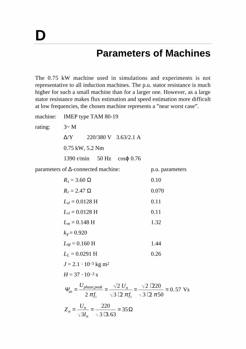
DParameters of Machines
The 0.75 kW machine used in simulations and experiments is notrepresentative to all induction machines. The p.u. stator resistance is muchhigher for such a small machine than for a larger one. However, as a largestator resistance makes flux estimation and speed estimation more difficultat low frequencies, the chosen machine represents a ”near worst case”.
machine: IMEP type TAM 80-19
rating: 3~ M
∆/Y 220/380 V 3.63/2.1 A
0.75 kW, 5.2 Nm
1390 r/min 50 Hz cosϕ 0.76
parameters of ∆-connected machine: p.u. parameters
Rs = 3.60 Ω 0.10
Rr = 2.47 Ω 0.070
Lsl = 0.0128 H 0.11
Lrl = 0.0128 H 0.11
Lm = 0.148 H 1.32
kγ = 0.920
LM = 0.160 H 1.44
LL = 0.0291 H 0.26
J = 2.1 · 10–3 kg m2
H = 37 · 10–3 s
Ψsn =Uphase,peak
2 π f1
= 2 Un
3 ⋅ 2 π f1
= 2 ⋅ 220
3 ⋅ 2 π 50= 0.57 Vs
Zn = Un
3In
= 220
3 ⋅3.63= 35Ω

EObserver Poles
The dynamic behaviour of the observer described by equation (4.12) isdetermined by the poles of the system. The poles are eigenvalues of thesystem matrix A e − Re k Ce( ) and can be calculated as the roots of thecharacteristic polynomial
P s( ) = det sI − A e − Re k Ce( )( ) (E.1)
where I is the identity matrix. Equations (E.1), (4.5), (4.7), (4.10) and(4.11) give
P s( ) = s2 + Rse ks + 1( ) 1
L Me
+ 1
L Le
+
R re 1 − kr( )L Le
− jzp ω
s
+Rse ks + 1( ) R re − jzp ω L Le + L Me( )( )
L Le + L Me
(E.2)
The required observer gain k for a desired characteristic polynomial,
P s( ) = s2 + c1s + c2 (E.3)
with the poles p1 and p2 where
c1 = − p1 + p2( ) (E.4)
c2 = p1 p2 (E.5)
is found with the following relation (Åström et al, 1984),
k = Re−1K
= Re−1P A e( )Wo
−1 0
1
= Re−1 A e
2 + c1A e + c2I( )Wo−1 0
1
= Re−1 A e
2 − p1 + p2( )A e + p1p2I( )Wo−1 0
1
(E.6)
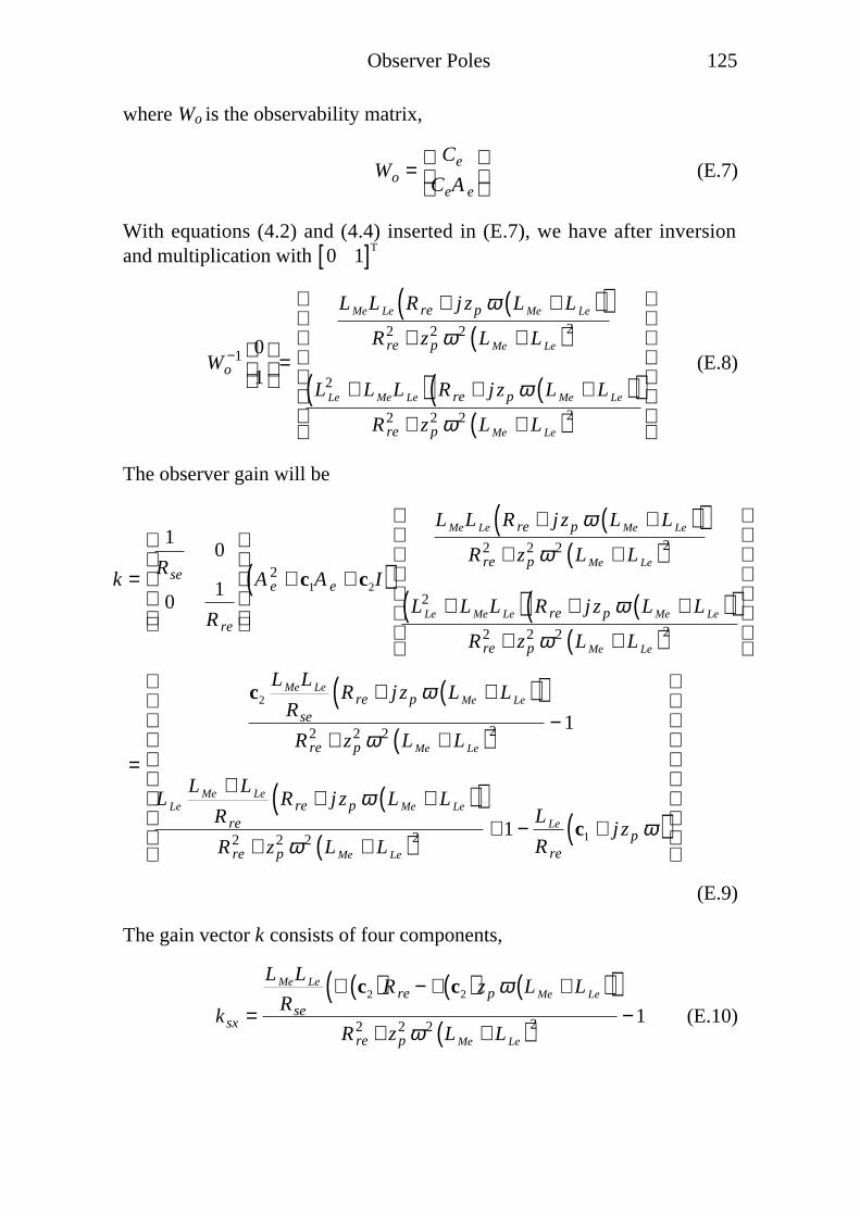
Observer Poles 125
where Wo is the observability matrix,
Wo =Ce
CeA e
(E.7)
With equations (4.2) and (4.4) inserted in (E.7), we have after inversionand multiplication with 0 1[ ]T
Wo−1 0
1
=
L MeL Le R re + j zp ω L Me + L Le( )( )R re
2 + zp2 ω 2 L Me + L Le( )2
L Le2 + L MeL Le( ) R re + j zp ω L Me + L Le( )( )
R re2 + zp
2 ω 2 L Me + L Le( )2
(E.8)
The observer gain will be
k =
1
Rse
0
01
R re
A e2 + c1A e + c2I( )
L MeL Le R re + j zp ω L Me + L Le( )( )R re
2 + zp2 ω 2 L Me + L Le( )2
L Le2 + L MeL Le( ) R re + j zp ω L Me + L Le( )( )
R re2 + zp
2 ω 2 L Me + L Le( )2
=
c2
L MeL Le
Rse
R re + j zp ω L Me + L Le( )( )R re
2 + zp2 ω 2 L Me + L Le( )2 − 1
L Le
L Me + L Le
R re
R re + j zp ω L Me + L Le( )( )R re
2 + zp2 ω 2 L Me + L Le( )2 + 1 − L Le
R re
c1 + j zp ω( )
(E.9)
The gain vector k consists of four components,
ksx =
L MeL Le
Rse
ℜ c2( )R re − ℑ c2( )zp ω L Me + L Le( )( )R re
2 + zp2 ω 2 L Me + L Le( )2 − 1 (E.10)

126 Observer Poles
ksy =
L MeL Le
Rse
ℑ c2( )R re + ℜ c2( )zp ω L Me + L Le( )( )R re
2 + zp2 ω 2 L Me + L Le( )2 (E.11)
k rx =L Le
L Me + L Le
R re
ℜ c2( )R re − ℑ c2( )zp ω L Me + L Le( )( )R re
2 + zp2 ω 2 L Me + L Le( )2 + 1 − L Le
R re
ℜ c1( )
(E.12)
k ry =L Le
L Me + L Le
R re
ℑ c2( )R re + ℜ c2( )zp ω L Me + L Le( )( )R re
2 + zp2 ω 2 L Me + L Le( )2 − L Le
R re
ℑ c1( ) + zp ω( )
(E.13)
Poles of System with Complex Variables
The observer system matrix A e − Re k Ce( ) is a 2 × 2 matrix with complexcoefficients. As the coefficients are complex, complex eigenvalues of thismatrix need not be complex conjugates. For a 2 × 2 matrix with realcoefficients on the other hand, complex eigenvalues come in pairs ofcomplex conjugates.
The observer can also be described with a 4 × 4 matrix with realcoefficients. If the observer is described by the real state vector
Ψsx
Ψrx
Ψsy
Ψry
instead of the complex state vector
ÁÁs
ÁÁr
the new observer have the following 4 × 4 system matrix
Observer Poles 127
ℜ A e − Re k Ce( ) −ℑ A e − Re k Ce( )
ℑ A e − Re k Ce( ) ℜ A e − Re k Ce( )
with real coefficients. The eigenvalues of this matrix are the same as theeigenvalues of A e − Re k Ce( ), but there are also two new eigenvalueswhich are the conjugates of the old ones.

FSteady State Value of Speed
Observer
The following steps give the solution to the system of equations (5.32)–(5.34). The first two equations can be written
ÁÁs jω1 + Rse 1 + ks( ) 1
L Me
+ 1
L Le
− ÁÁrRse 1 + ks( ) 1
L Le
= us + Rseksis
(F.1)
ÁÁs R rekr1
L Me
+ 1
L Le
− R re
L L
+ ÁÁr jω1 − jzpω + 1 − kr( ) R re
L Le
= R rekris
(F.2)
Introduce a, b, c, d, e and f to make the equations more compact,
aÁÁs + bÁÁr = c (F.3)
d ÁÁs + e − jzpω( )ÁÁr = f (F.4)
solving this system for the stator and rotor flux estimates gives thefunctions f1 and f2 of equations (5.38) and (5.39),
ÁÁs = f1 ω( ) =
ce − jczpω − bf
ae − jazpω − bd(F.5)
ÁÁr = f2 ω( ) = af − dc
ae − jazpω − bd(F.6)
Inserting this in equation (5.40), and some rearranging give
ç =af − dc + LLeis ae − bd( ) − LLeisjazpω
ce − bf − jczpω= n − mω
h − pω(F.7)
As ç is real, it follows that

Steady State Value of Speed Observer 129
ℑ n − mωh − pω
= 0
⇔
ℜ n − mω( )ℜ h − pω( )
=ℑ n − mω( )ℑ h − pω( )
⇔
nx − mxωhx − pxω
=ny − myωhy − pyω
(F.8)
where index x denotes real parts and index y denotes imaginary parts. Theestimated speed ω can now be calculated from this equation of the secondorder. The two solutions are
ω =hymx + pynx − hxmy − pxny
2 pymx − pxmy( )
+hymx + pynx − hxmy − pxny( )2
− 4 pymx − pxmy( ) hynx − hxny( )2 pymx − pxmy( )
(F.9)
and
ω =hymx + pynx − hxmy − pxny
2 pymx − pxmy( )
−hymx + pynx − hxmy − pxny( )2
− 4 pymx − pxmy( ) hynx − hxny( )2 pymx − pxmy( )
(F.10)
where

130 Steady State Value of Speed Observer
n = af − dc + L Lis ae − bd( )
= usR re1
L Le
− kr1
L Me
+ 1
L Le
+ is krRseR re1
L Me
+ 1
L Le
+ ksRseR re
1
L Le
+ jω1 R re − L Leω12
+ is jω1RseL Le 1 + ks( ) 1
L Me
+ 1
L Le
+ 1 + ks( )RseR re
1
L Me
(F.11)
m = jzp L Leisa = jzp L Leis jω1 + Rse 1 + ks( ) 1
L Me
+ 1
LLe
(F.12)
h = ce − bf
= jω1 us + jω1 Rseisks + R re
L Le
us 1 − kr( ) + Rseis ks + kr( )( ) (F.13)
p = jzpc = jzp us + Rseisks( ) (F.14)

GNon-linear Systems and Linearized
Systems
A few simple examples will demonstrate that linearization and calculationof poles of non-linear systems must be done with great caution.
Stability of Non-linear Systems
The non-linear system
dx
dt= x2 + x + u
y = x(G.1)
where u is the input and y is the output will be used to demonstrate sometraps. In this example, the input is
u = 0.5sin 10t( ) (G.2)
A linearized approximation of the system can be obtained if x is replacedby x 0 + δx ,
x = x 0 + δx (G.3)
where δx is the deviation from an operating point x 0 . As x 0 is constant itfollows that
dx 0
dt= 0 (G.4)
and
d
dtδx = dx
dt
= x 0 + δx( )2 + x 0 + δx + u
= x 02 + 2x 0δx + δx 2 + x 0 + δx + u
= 2x 0 + 1( )δx + x 0 + x 02 + δx 2 + u
(G.5)
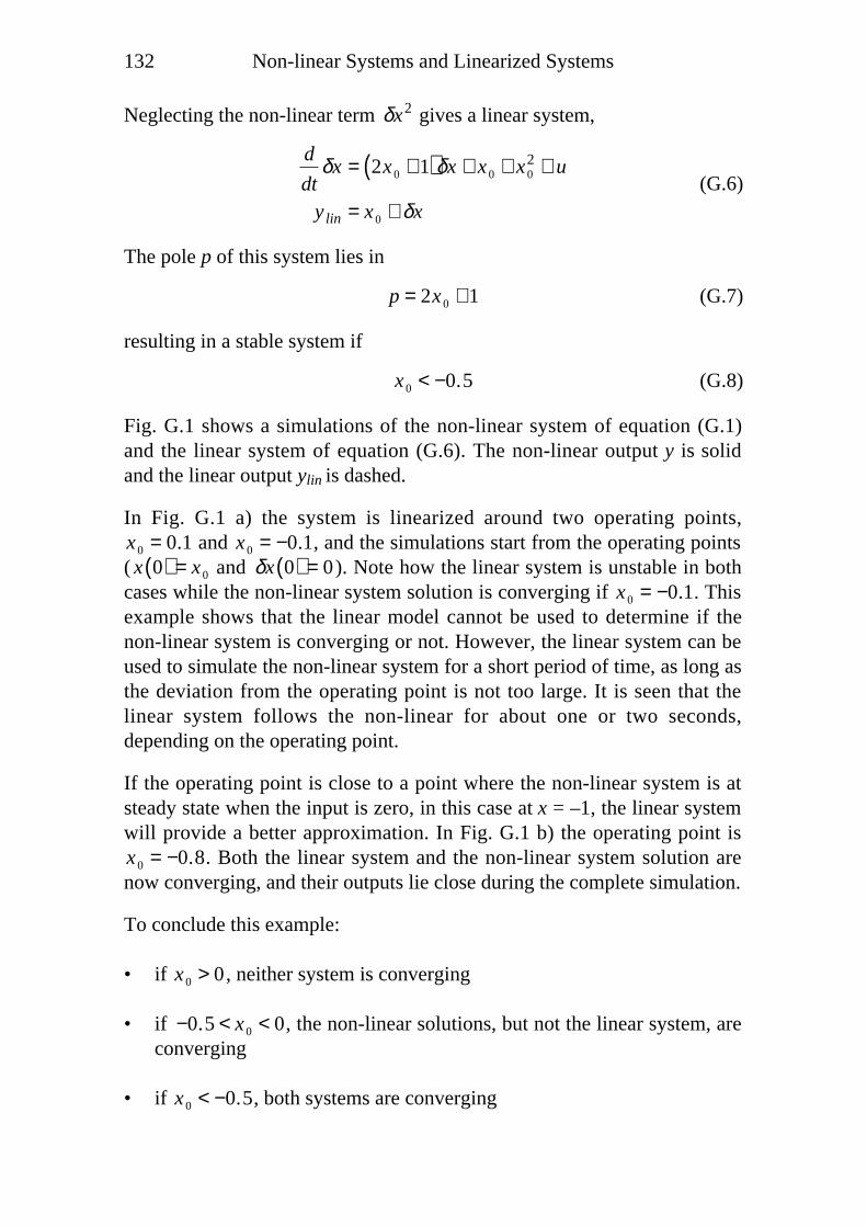
132 Non-linear Systems and Linearized Systems
Neglecting the non-linear term δx2 gives a linear system,
d
dtδx = 2x 0 + 1( )δx + x 0 + x 0
2 + u
ylin = x 0 + δx(G.6)
The pole p of this system lies in
p = 2x 0 + 1 (G.7)
resulting in a stable system if
x 0 < −0.5 (G.8)
Fig. G.1 shows a simulations of the non-linear system of equation (G.1)and the linear system of equation (G.6). The non-linear output y is solidand the linear output ylin is dashed.
In Fig. G.1 a) the system is linearized around two operating points,x 0 = 0.1 and x 0 = −0.1, and the simulations start from the operating points( x 0( ) = x 0 and δx 0( ) = 0 ). Note how the linear system is unstable in bothcases while the non-linear system solution is converging if x 0 = −0.1. Thisexample shows that the linear model cannot be used to determine if thenon-linear system is converging or not. However, the linear system can beused to simulate the non-linear system for a short period of time, as long asthe deviation from the operating point is not too large. It is seen that thelinear system follows the non-linear for about one or two seconds,depending on the operating point.
If the operating point is close to a point where the non-linear system is atsteady state when the input is zero, in this case at x = –1, the linear systemwill provide a better approximation. In Fig. G.1 b) the operating point isx 0 = −0.8. Both the linear system and the non-linear system solution arenow converging, and their outputs lie close during the complete simulation.
To conclude this example:
• if x 0 > 0 , neither system is converging
• if −0.5 < x 0 < 0, the non-linear solutions, but not the linear system, areconverging
• if x 0 < −0.5, both systems are converging
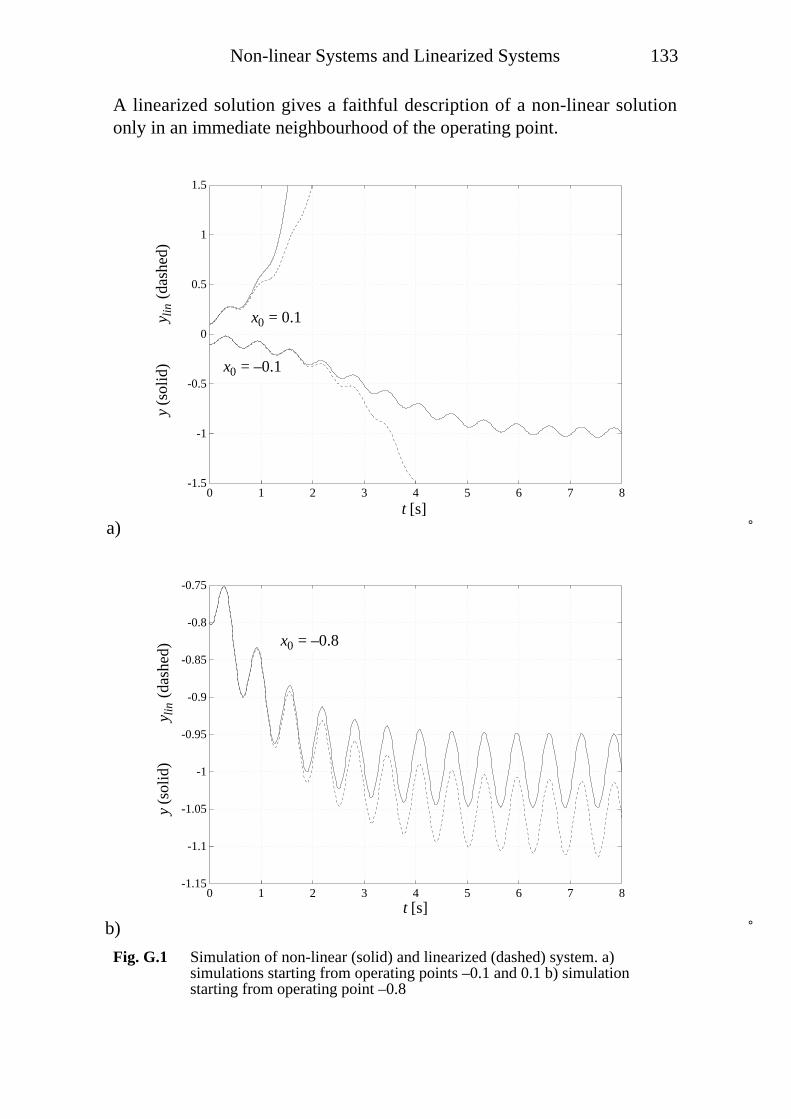
Non-linear Systems and Linearized Systems 133
A linearized solution gives a faithful description of a non-linear solutiononly in an immediate neighbourhood of the operating point.
a)
-1.5
-1
-0.5
0
0.5
1
1.5
0 1 2 3 4 5 6 7 8
t
solid
: x
da
shed
: x0+
delta
xx0=-0.1 and x0=0.1
x0 = –0.1
x0 = 0.1
y (s
olid
)
y lin
(da
shed
)
t [s]
b)
-1.15
-1.1
-1.05
-1
-0.95
-0.9
-0.85
-0.8
-0.75
0 1 2 3 4 5 6 7 8
t
solid
: x
da
shed
: x0+
delta
x
x0=-0.8
x0 = –0.8
y (s
olid
)
y lin
(da
shed
)
t [s]
Fig. G.1 Simulation of non-linear (solid) and linearized (dashed) system. a)simulations starting from operating points –0.1 and 0.1 b) simulationstarting from operating point –0.8

134 Non-linear Systems and Linearized Systems
Non-linearities Introduced by Change of Reference Frame
A linear system with the complex state variable x = x x + j x y described by
d
dt
xx
xy
=
−k 0
0 −k
xx
xy
+
ux
uy
(G.9)
will be used as an example to demonstrate some consequences of changingthe reference frame. The system is shown as a block diagram in Fig. G.2.
+–
k
ux xx∫
–+
k
uyxy
∫
−k 0
0 −k
u x
system in stationary frameb)
a)
Fig. G.2 Block diagram of a system in a stationary reference frame. a) detail b)overview.
Both poles of this system are equal and real-valued,
p1,2 = −k (G.10)
Let the input u = ux + juy be rotating with angular velocity ω1,
ux
uy
=
u cosω1t
usin ω1t
(G.11)

Non-linear Systems and Linearized Systems 135
After the transient, the state x will also be rotating with angular velocity ω1.If instead the reference frame is rotating synchronously with the input u,the system is described by equation
d
dt
xxr
xyr
=−k ω1
−ω1 −k
xxr
xyr
+ux
r
uyr
(G.12)
where the r-superscripts denote quantities in the rotating frame. The systemis also shown as a block diagram in Fig. G.3.
++–
k
ux xx∫
––+
k
uy
xy∫
u x
r r
r
r
ω1
−k ω1
−ω1 −k
r ru xcosω1t sin ω1t
−sin ω1t cosω1t
cosω1t −sin ω1t
sin ω1t cosω1t
transformation matrix system in rotating frame transformation matrixb)
a)
ω1
Fig. G.3 Block diagram of a system in a rotating reference frame. a) detail b)overview.
Any vector v = vx + jvy in the stationary frame can be transformed to therotating frame with the following relation,
vxr
vyr
=cosω1t sin ω1t
−sin ω1t cosω1t
vx
vy
(G.13)
The real and imaginary parts of the input ur = uxr + juy
r will be constant inthe rotating frame,
136 Non-linear Systems and Linearized Systems
uxr
uyr
=cosω1t sin ω1t
−sin ω1t cosω1t
u cosω1t
usin ω1t
=u
0
(G.14)
and also the state xr = xxr + jxy
r will be constant after the transient. If thisstate is transformed back to the stationary frame as in Fig. G.3 b), using atransformation matrix which is the inverse of the matrix in equation (G.13),
xx
xy
=
cosω1t −sin ω1t
sin ω1t cosω1t
xxr
xyr
(G.15)
x = x x + j x y will be rotating with angular velocity ω1. After thetransformations, the outputs of both the system in Fig. G.2 and the systemin Fig. G.3 will be identical. However, the system in the rotating framehave its poles in
p1,2 = −k ± jω1 (G.16)
Here we have two systems with the same behaviour, but one of the systemshas its poles on the real axis, indicating a well damped system, while thepoles of the other system have moved a distance ω1 from the real axis,indicating a system with less damping. The explanation is that thetransformation from the stationary reference frame to the rotating frameintroduces a non-linearity to the system. In Fig. G.3 it is seen that states, xx
and xy are multiplied by an input variable ω1. As the angular frequency ofthe input u might be changing, ω1 should be considered an input, and not aconstant. The poles are meaningful only for a linear system, i.e. if ω1 isheld constant. Such a limitation does not exist for the system in thestationary frame. The conclusion is that even though equation (G.9) and(G.12) describe the same physical system, the first equation is a lineardescription, while the second equation is non-linear.