indifferentiability security of the fast widepipe hash

Indifferentiability Security of the Fast Wide Pipe Hash: Breaking the Birthday Barrier

Dustin Moody∗ Souradyuti Paul† Daniel Smith-Tone‡

Abstract A hash function secure in the indifferentiability framework (TCC 2004) is able to

resist all meaningful generic attacks. Such hash functions also play a crucial role in establishing the security of protocols that use them as random functions.

To eliminate multi-collision type attacks on the Merkle-Damgård mode (Crypto 1989), Lucks proposed widening the size of the internal state of hash functions. More specifically, he suggested that hash functions h : {0, 1}∗ → {0, 1}n use underlying primitives of the form C : {0, 1}a → {0, 1}2n (Asiacrypt 2005). The Fast Wide Pipe (FWP) hash mode was introduced by Nandi and Paul at Indocrypt 2010, as a faster variant of Lucks’ Wide Pipe mode. Despite the higher speed, the proven indifferentiability bound of the FWP mode has so far been only up to the birthday barrier of n/2 bits. The main result of this paper is the improvement of the FWP bound to 2n/3 bits (up to an additive constant).

The 2n/3-bit bound for FWP comes with two important implications. Many popular hash modes use primitives with a = 2n, that is C : {0, 1}2n → {0, 1}2n. For this important case, the FWP becomes the only mode to achieve indifferentiability security of more than n/2 bits; thus we solve a longstanding open problem. Secondly, among n-bit hash modes with a > 2n, the FWP mode has the highest rate among all modes which have beyond-birthday-barrier security.

To obtain the bound of 2n/3 bits, we follow the usual technique of constructing games with simulators, with certain BAD events to distinguish between the games. However, we introduce some novel ideas. In designing the BAD events, we used multi-collisions in addition to collisions. We also allowed the query-response graphs, maintained by the simulators, to grow for two phases every iteration, rather than just one phase. Finally, our carefully chosen set of sixteen BAD events establish an isomorphism of simulator graphs, from which the 2n/3-bit bound follows.

We also provide evidence that extending the bound beyond 2n/3 bits may be possible if we allow the simulator-graph to grow for three (or more) phases every iteration. Another noteworthy feature of our proof – that may be of independent interest – is that we work with only three games rather than a long sequence games.

Keywords: Indifferentiability, birthday barrier, Fast wide pipe.

∗NIST, Computer Security Div. USA, [email protected] †Univ. of Waterloo, Math Dept., Canada and K. U. Leuven, Belgium, [email protected] ‡NIST, USA, and Univ. of Louisville, Math Dept., KY, USA, [email protected]

1

mailto:[email protected]



Contents

Page

1 Introduction 5 1.1 Motivation . . . . . . . . . . . . . . . . . . . . . . . . . . . . . . . . . . . . 5 1.2 Our contribution . . . . . . . . . . . . . . . . . . . . . . . . . . . . . . . . . 7

2 Preliminaries 9 2.1 Notation and convention . . . . . . . . . . . . . . . . . . . . . . . . . . . . . 9 2.2 Description of FWP mode . . . . . . . . . . . . . . . . . . . . . . . . . . . . 10 2.3 Indifferentiability framework . . . . . . . . . . . . . . . . . . . . . . . . . . . 10

3 Main Theorem: Beyond-birthday-barrier Security of FWP 11 3.1 Proof of Theorem 3.1: outline . . . . . . . . . . . . . . . . . . . . . . . . . . 12 3.2 Organization . . . . . . . . . . . . . . . . . . . . . . . . . . . . . . . . . . . 13

4 Data Structures 13 4.1 Objects used in pseudocode . . . . . . . . . . . . . . . . . . . . . . . . . . . 13

4.1.1 Oracles . . . . . . . . . . . . . . . . . . . . . . . . . . . . . . . . . . 13 4.1.2 Global and local variables . . . . . . . . . . . . . . . . . . . . . . . . 13 4.1.3 Query and round: definitions . . . . . . . . . . . . . . . . . . . . . . 13

4.2 Graph theoretic objects used in proof of main theorem . . . . . . . . . . . . 14 4.2.1 Reconstructible message . . . . . . . . . . . . . . . . . . . . . . . . . 14 4.2.2 (Full) Reconstruction graph . . . . . . . . . . . . . . . . . . . . . . . 15 4.2.3 View . . . . . . . . . . . . . . . . . . . . . . . . . . . . . . . . . . . . 15

5 Main system G0 17

6 Main system G2 17 6.1 Intuition for simulator S . . . . . . . . . . . . . . . . . . . . . . . . . . . . . 17 6.2 Detailed description of simulator S . . . . . . . . . . . . . . . . . . . . . . . 18

7 Intermediate system G1 19 7.1 Motivation . . . . . . . . . . . . . . . . . . . . . . . . . . . . . . . . . . . . 19 7.2 Detailed description of G1 . . . . . . . . . . . . . . . . . . . . . . . . . . . . 20

8 First Part of Main Theorem: Proof of (2) 22

9 Type0, 1, 2, and 3, of System G1 22 9.1 Motivation . . . . . . . . . . . . . . . . . . . . . . . . . . . . . . . . . . . . 22 9.2 Classifying elements of Dro, branches of Tro, and ro-queries . . . . . . . . . 22

9.2.1 Elements of Dro: six types . . . . . . . . . . . . . . . . . . . . . . . . 25

2

9.2.2 Branches of Tro: four types . . . . . . . . . . . . . . . . . . . . . . . 25 9.2.3 The ro-queries: seven types . . . . . . . . . . . . . . . . . . . . . . . 25

9.3 Definition: Type0 and Type1 on fresh queries . . . . . . . . . . . . . . . . . 26 9.3.1 Intuition . . . . . . . . . . . . . . . . . . . . . . . . . . . . . . . . . . 26 9.3.2 Type0 event: collision in outputs of ro . . . . . . . . . . . . . . . . . 28 9.3.3 Type1 event: collision in Tro . . . . . . . . . . . . . . . . . . . . . . . 28

9.4 Type2 and Type3 on old queries . . . . . . . . . . . . . . . . . . . . . . . . 29 9.4.1 Intuition . . . . . . . . . . . . . . . . . . . . . . . . . . . . . . . . . . 29 9.4.2 Type2 . . . . . . . . . . . . . . . . . . . . . . . . . . . . . . . . . . . 29 9.4.3 Type3 . . . . . . . . . . . . . . . . . . . . . . . . . . . . . . . . . . . 30

10 Second Part of Main Theorem: Proof of (3) 30 10.1 Definitions: GOODi and BADi . . . . . . . . . . . . . . . . . . . . . . . . . . 30 10.2 Proof of (3) . . . . . . . . . . . . . . . . . . . . . . . . . . . . . . . . . . . . 31

11 A Few Combinatorial Results 31

12 Third (or Final) Part of Main Theorem: Proof of (4) 35 12.1 Estimating probability of Type0i . . . . . . . . . . . . . . . . . . . . . . . . 35 12.2 Estimating probability of Type1i . . . . . . . . . . . . . . . . . . . . . . . . 36

12.2.1 Computing probability of Type1-ai . . . . . . . . . . . . . . . . . . . 36 12.2.2 Computing probability of Type1-bi . . . . . . . . . . . . . . . . . . . 37 12.2.3 Computing probability of Type1-ci . . . . . . . . . . . . . . . . . . . 37 12.2.4 Computing probability of Type1-di . . . . . . . . . . . . . . . . . . . 37 12.2.5 Computing probability of Type1-ei . . . . . . . . . . . . . . . . . . . 38 12.2.6 Computing probability of Type1-fi . . . . . . . . . . . . . . . . . . . 39 12.2.7 Final summation . . . . . . . . . . . . . . . . . . . . . . . . . . . . . 39

12.3 Estimating probability of Type2i . . . . . . . . . . . . . . . . . . . . . . . . 39 12.3.1 Estimating probability of Type2-ai . . . . . . . . . . . . . . . . . . . 40 12.3.2 Estimating probability of Type2-bi . . . . . . . . . . . . . . . . . . . 40 12.3.3 Estimating probability of Type2-ci . . . . . . . . . . . . . . . . . . . 40 12.3.4 Estimating probability of Type2-di . . . . . . . . . . . . . . . . . . . 40 12.3.5 Estimating probability of Type2-ei . . . . . . . . . . . . . . . . . . . 41 12.3.6 Estimating probability of Type2-fi . . . . . . . . . . . . . . . . . . . 41 12.3.7 Final summation . . . . . . . . . . . . . . . . . . . . . . . . . . . . . 41

12.4 Estimating probability of Type3i . . . . . . . . . . . . . . . . . . . . . . . . 41 12.4.1 Estimating probability of Type3-ai . . . . . . . . . . . . . . . . . . . 41 12.4.2 Estimating probability of Type3-bi . . . . . . . . . . . . . . . . . . . 42 12.4.3 Estimating probability of Type3-ci . . . . . . . . . . . . . . . . . . . 42 12.4.4 Final summation . . . . . . . . . . . . . . . . . . . . . . . . . . . . . 42

12.5 Final step . . . . . . . . . . . . . . . . . . . . . . . . . . . . . . . . . . . . . 42

3

42 13 Experimental Results: The Bound Improves Towards n bits

14 Conclusion and Open Problems 43

A Definitions 49

B WP and FWP 50

C Time costs of FullGraph and simulator S 50

D Six Types of ro-query-response Pairs 50

E Proof of (8) 51

4

1 Introduction

1.1 Motivation

Iterative hash functions are usually composed of two parts: (1) a basic primitive C with finite domain and range, and (2) an iterative mode of operation H to extend the domain of C. In studying the security of a hash function, both the security of the primitive C, as well as the security of the mode of operation H need to be examined separately, since the hash function can be attacked by breaking either C or the mode H. Our focus is on the security of the hash mode H. Throughout the paper we would assume that the primitive C is an ideal object, that is, it does not exhibit any non-trivial weakness.

Generic attacks on hash modes. In a generic attack, an adversary attempts to break a property of a hash mode assuming the underlying primitive is an ideal object, such as a random oracle, an ideal permutation, or an ideal cipher. For example, suppose the hash function h : {0, 1}∗ → {0, 1}n, for a given input M ∈ {0, 1}∗, invokes a random oracle ro : {0, 1}a → {0, 1}b, one or multiple times, to compute h(M). Informally, a generic attack breaks a property of the hash function h (e.g. 1st/2nd pre-image, collision resistance) utilizing less resources than would be required to break the same property of the random oracle RO : {0, 1}∗ → {0, 1}n .

Generic attacks against hash modes are abundant in the literature. See, for example, Joux’s multi-collision attack [23], Kelsey-Schneier expandable message attack [25], or Kelsey-Kohno herding attack [24, 11], among others [1, 9, 22, 32].

Indifferentiability security. The indifferentiability security framework was introduced by Maurer et al.[27] in 2004, and was first applied to analyze hash modes of operation by Coron et al.[17] in 2005. A hash mode proven secure in this framework is able to resist all generic attacks. More technically, the indifferentiability framework measures the extent to which a hash function behaves as a random oracle under the assumption that the underlying small compression function is an ideal object. Indifferentiability attacks include more attacks [3, 9, 15] than just those with known practical significance. Thus in some sense, an indifferentiable hash function can be viewed as eliminating potential future attacks. We note that the security of many cryptographic protocols (e.g. RSA-OAEP [34], RSA-PSS [16]) relies on the indifferentiability security of the underlying hash functions that the protocols use as random oracles. In such a case, the security of the hash functions against specialized attacks – such as collision, 1st/2nd pre-image attacks – is inadequate to guarantee the security of the overlying protocol. As a result, most new proposals for hash modes of operation include indifferentiability proofs of security. We note that some limitations of the indifferentiability framework have recently been discovered in [19] and [33]. These limitations, nevertheless, do not affect the proven security bounds of hash functions based on ideal objects.

5

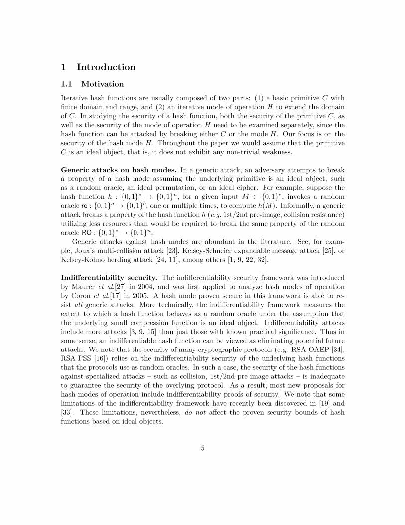
Mode of operation

Primitive input (a)

Message block (.)

Rate (./a)

Indiff. bound Primitive lower upper

1. WP,chopMD [14, 17] 2n 0 0 0 0 ro 2. JH [30] 2n n 0.5 n/2 n(1 − E) ip 3. Grøstl [20] 2n n 0.5 n/2 n ip 4. Sponge [8] 2n n 0.5 n/2 n/2 ip 5. Parazoa [5] 2n n 0.5 up to n/2 n ip 6. FWP (this paper) 2n n 0.5 2n/3 n ro

7. Shabal [13] 4n n 0.25 n n ic 8. BLAKE [2, 15] 4n 2n 0.5 n/2 n/2 ic

9. FWP (this paper) 4n 3n 0.75 2n/3 n ro

10. WP,chop MD [14, 17] t + 2n t t/(t + 2n) n n ro

11. FWP (this paper) t + 2n t + n (t + n)/(t + 2n) 2n/3 n ro

Table 1: Indifferentiability security bounds (upper and lower) for several wide-pipe hash modes, where the primitive output is 2n-bit (the hash size is n-bit). The primitives ro, ic and ip are shorthand for random oracle, ideal cipher, and ideal permutation. The letter t denotes a positive integer. The E is a small fraction due to the preimage attack on JH presented in [9].

Advantages of primitives with 2n-bit output. Many practical iterative hash modes which use primitives with n-bit output have been shown to come under multi-collision attacks with O(2n/2) queries [23]. Therefore, their indifferentiability security bounds cannot be extended beyond n/2 bits. A few well known examples include Merkle-Damgård [18, 29], HAIFA [10], EMD [6], and MDP [21].

As a result, to design a practical hash mode with indifferentiability security more than n/2 bits, it seems necessary to use primitives with 2n bits of output (or more) [26]. Examples of hash modes with 2n bits of output include: Wide Pipe-MD [26], FWP [31], JH [36], Grøstl [20], Sponge [8], Shabal [13], and Parazoa [5], to name a few.

The rate of a hash function. In any iterative hash function h : {0, 1}∗ → {0, 1}n, the input to the underlying primitive C : {0, 1}a → {0, 1}b is composed of an .-bit message block and an (a − .)-bit chaining value from the previous iteration. It is easy to see that, for a fixed a and b, the higher the value of ., the faster the hash computation. To formalize this property, we define the rate of a hash function as the ratio ./a, where . is the (average) length of a message block.1

1The average length of a message block is computed as the length of a padded message divided by the total number of invocations of the primitive(s). This addresses the issue when the same message block is used in multiple invocations of the primitive (e.g. Grøstl).

6

The challenge. Based on the previous discussion, the challenge is to design an n-bit hash function using primitives of the form C : {0, 1}a → {0, 1}2n which maximize both the rate and the indifferentiability security bound. The rates and security bounds of several hash modes with primitive output 2n-bit have been tabulated in Table 1.

1.2 Our contribution

IV

m1 m2 m3 mk−1 mk

hIV ′C C C C C

` ` ` ` `− n

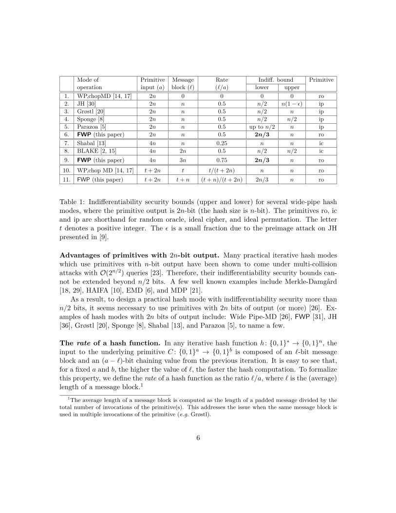
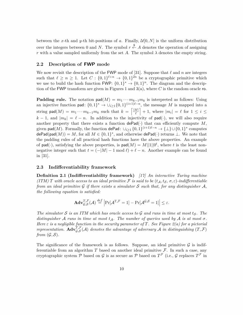
Figure 1: Diagram of the FWP mode. All unlabeled wires are n bits each. The shaded region is viewed as compression function.

The FWP mode (2010). The Fast Wide Pipe (FWP) hash mode was proposed by Nandi and Paul in 2010 [31], as a faster variant of the Wide Pipe (WP) mode [26] (see Figure 1). The key idea used in FWP is that only half of the chaining value – instead of the full chaining value – is used as input into the primitive C, while the other half is XOR-ed into the output. Thus, FWP increases the rate by allowing message blocks larger than those used by the WP mode. See Figure 11 of Appendix B, which compares the WP mode with the FWP mode. As is the case with all other high rate hash modes with primitive output 2n bits, the indifferentiability bound of FWP has so far remained only up to n/2 bits [31].

The difficulty of breaking the birthday-barrier. It is apparent from Table 1 that extending both the rate and the indifferentiability bound of a hash mode is a challenging task. Note that the Shabal and Wide Pipe modes have n-bit security bounds, but their rates are quite low. For the Sponge function – though having a high rate of 0.5 – the security bound is n/2-bit, which cannot be improved further, since there is a preimage attack with work approximately 2n/2 [7].

Several other designs (JH (2007), Grøstl (2007), FWP (2010) and the Parazoa family (2011)) have shown promise. Each achieves the high rate of 0.5 (if a = 3n then the FWP can achieve a rate of 0.67), and their indifferentiability bounds can potentially be improved beyond the birthday barrier. Despite several attempts, so far none of them has been shown to have the beyond-birthday-barrier security. See [9], [30], [31] and [4].

7

In all of the previous attempts, the basic approach for proving indifferentiability security has been more or less the same. First, a suitable compression function is constructed around the primitive C. See, for example, the compression function contained in the shaded part of Figure 1. Then a set of events are identified that primarily consider collisions on n (out of 2n) bits of output of the compression function. These events are typically called BAD events, and are used to differentiate between pairs of games. Lastly, using some sophisticated combinatorial tricks and counting techniques, the total probability of the BAD events are computed by summing them across all rounds and messages.

The main deficiency in the above approach is two-pronged. The probability of the BAD events is dominated by the probability of n-bit collisions of the compression function output, which is too high. Considering n-bit collisions can only give a bound of n/2 bits. On the other hand, if we consider collisions on the 2n bits of the compression function

i2 output, then after i queries we end up having O reconstructible messages (defined later), and this will again lead to a bound only of n/2 bits.

Evidently to go beyond the n/2-bit security bound, we need to identify BAD events whose probability of occurrence will be as low as the probability of random 2n-bit collisions (rather than of n-bit collisions). We also need that the number of all reconstructible messages after i queries will be linear in i, rather than quadratic.

The main result. Our main results is the improvement of the indifferentiability security bound for the FWP mode from n/2 to 2n/3 bits (up to a constant factor). The FWP mode is based on a primitive of the form C : {0, 1}a → {0, 1}2n, and our 2n/3-bit security bound is valid for all a ≥ 2n. We make two important observations.

Let H(a, b, r) denote the class of all rate r, n-bit hash functions with a primitive of the form C : {0, 1}a → {0, 1}b. The FWP mode is the only known hash mode with the beyond-birthday-barrier security in the important class H(2n, 2n, 0.5). Compare FWP with JH, Grøstl, Sponge, and the Parazoa family. This essentially settles a longstanding open problem.

Let H̃(a, b) denote the class of all n-bit hash functions with the beyond-birthday-barrier security based upon primitives of the form C : {0, 1}a → {0, 1}b. In the important class H̃(a, 2n), the FWP mode achieves the highest rate for all a ≥ 2n. Compare FWP with chop-MD, Shabal and BLAKE.

The tools. The first new idea used to break the n/2-bit bound is in using certain 3-multicollisions on n bits – in addition to collisions on 2n bits – as potential BAD events. We show that the 3-multi-collisions on n bits as well as the 2n-bit collisions both occur with low probabilities. In particular, we carefully design a set of sixteen bad events defined on the query, primitive and compression function outputs.

The second trick is to split the above 2n-bit collisions into two distinct n-bit collisions occurring in two different phases at the time of updating the simulator’s graph (technically we shall call it a reconstruction graph). Updating the reconstruction graph – whose

8

branches represent messages built from the queries and their responses – in a sequence of two phases, rather than just one, is crucial to the results in this work.

Using these two techniques, we are able to overcome the aforementioned obstacles in moving beyond the n/2-bit bound. In particular, the absence of the BAD events allows the reconstruction graph to grow for a maximum of two phases every round, while restricting the number of newly added nodes in the graphs to a constant number. As a result, we have O(i) reconstructible messages after i rounds, and at the same time, the probability of occurrence of the BAD events remains low. Once these important requirements are fulfilled, the final step is to prove an isomorphism of graphs, which then directly implies the claimed bound.

Another feature of our work, which may be of independent interest, is that the proof of our main theorem requires only three games. Compare this with the usual practice of tackling such problems using a sequence of a large number of games. The smaller number of games – in our opinion – makes third-party verification of the proof a great deal easier. In addition, our proof technique can likely be used to improve the security analysis of other modes.

Beyond the 2n/3-bit barrier It seems likely that the 2n/3-bit bound of FWP could be further improved, if we switched from two phases to a three phase framework. We experimented with a slightly different set of BAD events in the three (or more) phase framework. The results provide ample evidence that the indifferentiability bound for the FWP mode can be stretched closer to n bits. We leave it as an open problem to complete the theoretical analysis required for such an improved bound.

Warning. As is necessary for any analysis of cryptosystems based on ideal objects, we caution the reader that the security guarantee of 2n/3 bits for any practical hash function, based on the FWP mode, can be achieved as long as the underlying concrete primitive is free from all structural weaknesses, about which the paper makes no claims.

2 Preliminaries

2.1 Notation and convention

Throughout the paper we let n be a fixed integer. While representing a bit-string, we follow the convention of low-bit first (or little-endian bit ordering). For concatenation of strings, we use a||b, or just ab if the meaning is clear. The symbol (n)m denotes the m-bit encoding of n. The symbol |x| denotes the bit-length of the bit-string x, or sometimes

parsethe size of the set x. Let x → x1x2 · · · xk means parsing x into x1, x2, · · · , xk such that |x1| = |x2| = · · · = |xk−1| = n and |xk| = |x|−|x1x2 · · · xk−1|. Let Dom(T ) = {i | T [i] = ⊥}and Rng(T ) = {T [i] | T [i] =⊥}. We write AB to denote an Algorithm A with oracle access to B. Let [c, d] be the set of integers between c and d inclusive, and a[x, y] the bit-string

9

between the x-th and y-th bit-positions of a. Finally, U [0, N ] is the uniform distribution $over the integers between 0 and N . The symbol r ← A denotes the operation of assigning

r with a value sampled uniformly from the set A. The symbol λ denotes the empty string.

2.2 Description of FWP mode

We now revisit the description of the FWP mode of [31]. Suppose that . and n are integers +nsuch that . ≥ n ≥ 1. Let C : {0, 1}1 → {0, 1}2n be a cryptographic primitive which

we use to build the hash function FWP: {0, 1}∗ → {0, 1}n. The diagram and the description of the FWP transform are given in Figures 1 and 3(a), where C is the random oracle ro.

Padding rule. The notation pad(M) = m1 · · · mk−1mk is interpreted as follows: Using an injective function pad : {0, 1}∗

string pad(M) ,

such that k = |M1

| → ∪i≥1{0, 1}(i+1)1−n, the message M is mapped into a

+ 1, where for 1| | ≤ ≤= imi .

In addition to the injectivity of pad(·), we will also require

= m1 · · · mk−1mk

k − 1, and |mk| = . − n. another property that there exists a function dePad(·) that can efficiently compute M , given pad(M). Formally, the function dePad : ∪i≥1 {0, 1}(i+1)1−n → {⊥}∪{0, 1}∗ computes dePad(pad(M)) = M , for all M ∈ {0, 1}∗, and otherwise dePad(·) returns ⊥. We note that the padding rules of all practical hash functions have the above properties. An example of pad(·), satisfying the above properties, is pad(M) = M ||1||0t, where t is the least nonnegative integer such that t = (−|M | − 1 mod .) + . − n. Another example can be found in [31].

2.3 Indifferentiability framework

Definition 2.1 (Indifferentiability framework) [17] An interactive Turing machine (ITM) T with oracle access to an ideal primitive F is said to be (tA, tS , σ, ε)-indifferentiable from an ideal primitive G if there exists a simulator S such that, for any distinguisher A, the following equation is satisfied:

(A) defAdvT,

G,SF =

Pr[AT,F = 1] − Pr[AG,S = 1] ≤ ε.

The simulator S is an ITM which has oracle access to G and runs in time at most tS . The distinguisher A runs in time at most tA. The number of queries used by A is at most σ. Here ε is a negligible function in the security parameter of T . See Figure 2(a) for a pictorial representation. AdvT,F (A) denotes the advantage of adversary A in distinguishing (T, F)G,S from (G, S).

The significance of the framework is as follows. Suppose, an ideal primitive G is indifferentiable from an algorithm T based on another ideal primitive F . In such a case, any cryptographic system P based on G is as secure as P based on T F (i.e., G replaces T F in

10

3

T F G S

A

System 1 System 2

A

FWP ro

G0

A

FWP1 S1

G1

ro

A

RO S

G2≡ 6≡

(a) (b)

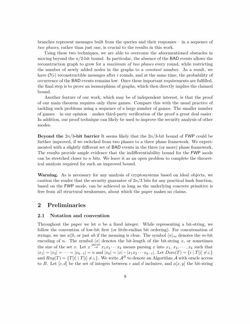
Figure 2: (a) Indifferentiability framework formalized in Definition 2.1. (b) Schematic diagrams of the security games – described in Section 3 – used in the indifferentiability framework for FWP. The arrows show the directions in which the queries are submitted.

P). For a more detailed explanation, we refer the reader to [28]. Some limitations of the indifferentiability framework have recently been discovered in [19] and [33]. They offer a deep insight into the framework; nevertheless, the observations are not known to affect the security of the indifferentiable hash functions in any meaningful way.

An oracle, a system, and a game. An oracle is an algorithm (accessed by another oracle or algorithm) which, given an input as an appropriately defined query, responds with an output. For example, in Figure 2(a), T , F , G and S are oracles. A system is a set of oracles (e.g. System 1 = (T, F), System 2 = (G, S) in Figure 2(a)). A game is the interaction of a system with an adversary. We refrain from providing a formal definition of a game, since such formalization will not be necessary in our analysis.

Main Theorem: Beyond-birthday-barrier Security of FWP

Let RO : {0, 1}∗ → {0, 1}n and ro : {0, 1}1+n → {0, 1}2n be two random oracles (see Appendix A for a definition).

Our indifferentiability framework uses three systems G0 = (FWP, ro), G1 = (FWP1, S1), and G2 = (RO, S) (see Figure 2(b)). The correspondence between the entities of Figures 2(a) and 2(b) are as follows: G = RO, T = FWP and F = ro. The description of FWP1, S, and S1 will be provided in Sections 5, 6, and 7.

Now we state our main theorem using Definition 2.1.

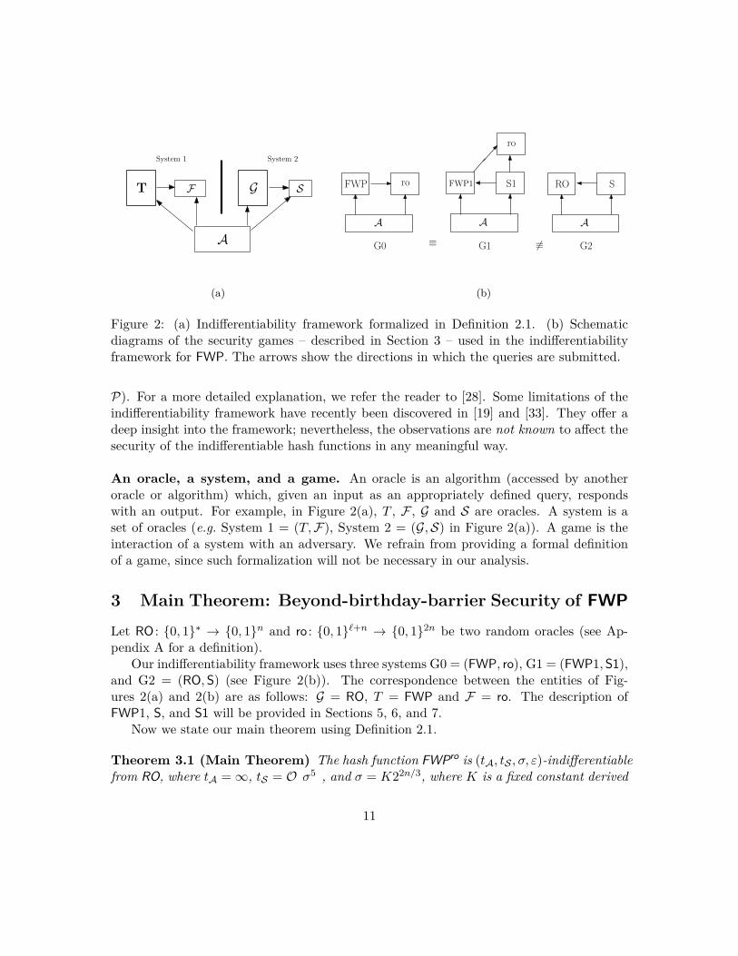
Theorem 3.1 (Main Theorem) The hash function FWPro is (tA, tS , σ, ε)-indifferentiable from RO, where tA = ∞, tS = O σ5 , and σ = K22n/3, where K is a fixed constant derived

11

from ε.

In the next few sections, we will prove Theorem 3.1 by breaking it into several components. First, we briefly describe what the theorem means: it says that no adversary with unbounded running time can mount a non-trivial generic attack on the hash function FWPro using at most K22n/3 queries. The parameter K is an increasing function in ε, and is constant for all n > 0, for a fixed ε. To reduce the notation complexity, we compute the √indifferentiability bound assuming ε = 1/2, for which, we shall derive K = 1/ 3 206.

3.1 Proof of Theorem 3.1: outline

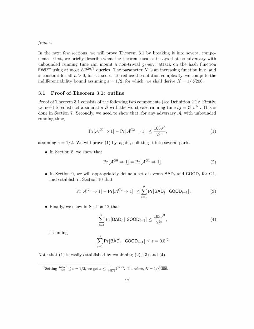
Proof of Theorem 3.1 consists of the following two components (see Definition 2.1): Firstly, we need to construct a simulator S with the worst-case running time tS = O σ5 . This is done in Section 7. Secondly, we need to show that, for any adversary A, with unbounded running time,

103σ3

Pr AG0 ⇒ 1 − Pr AG2 ⇒ 1 ≤ , (1)22n

assuming ε = 1/2. We will prove (1) by, again, splitting it into several parts.

• In Section 8, we show that Pr AG0 ⇒ 1 = Pr AG1 ⇒ 1 . (2)

• In Section 9, we will appropriately define a set of events BADi and GOODi for G1, and establish in Section 10 that

σ Pr AG1 ⇒ 1 − Pr AG2 ⇒ 1 ≤ Pr BADi | GOODi−1 . (3)

i=1

• Finally, we show in Section 12 that

σ 103σ3

Pr BADi | GOODi−1 ≤ , (4)22n i=1

assuming σ 2Pr BADi | GOODi−1 ≤ ε = 0.5.

i=1

Note that (1) is easily established by combining (2), (3) and (4).

3 √2Setting 103σ ≤ ε = 1/2, we get σ ≤ √1 22n/3 . Therefore, K = 1/ 3 206.22n 3 204

12

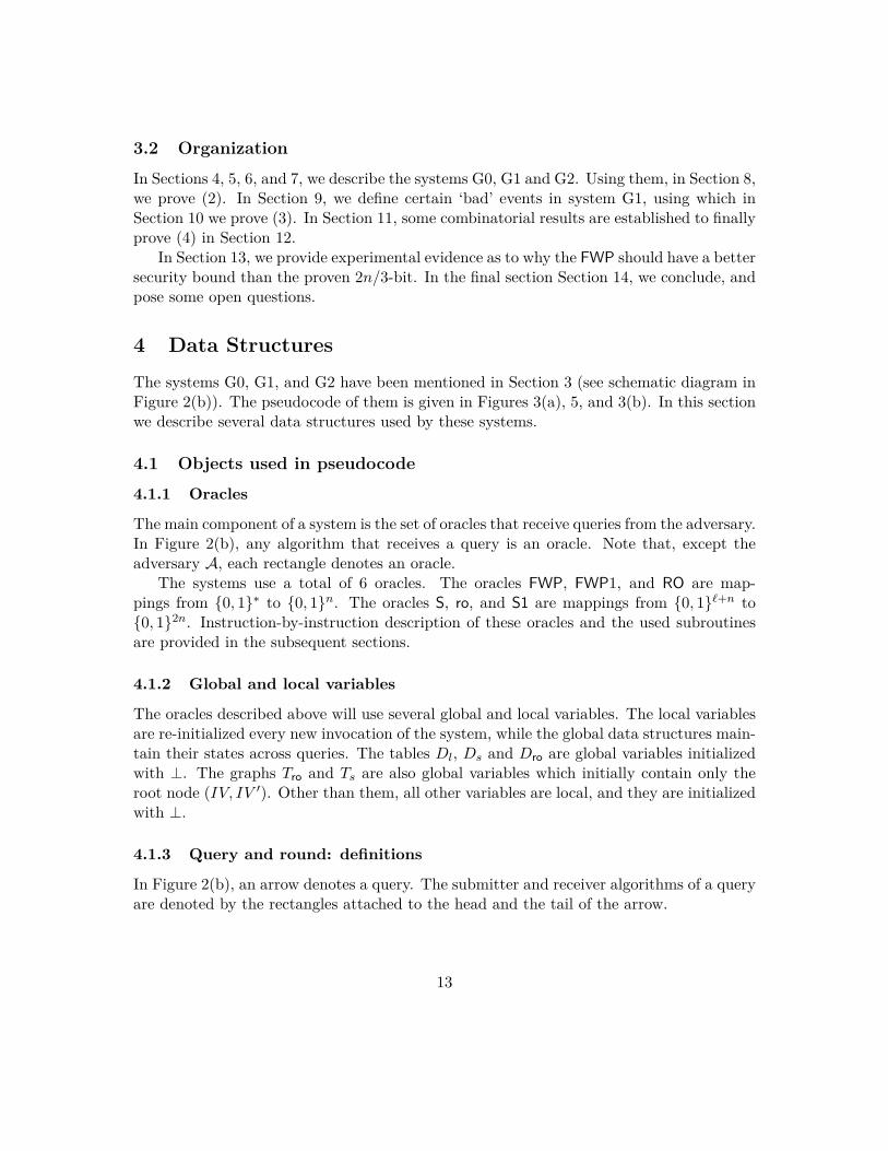
3.2 Organization

In Sections 4, 5, 6, and 7, we describe the systems G0, G1 and G2. Using them, in Section 8, we prove (2). In Section 9, we define certain ‘bad’ events in system G1, using which in Section 10 we prove (3). In Section 11, some combinatorial results are established to finally prove (4) in Section 12.

In Section 13, we provide experimental evidence as to why the FWP should have a better security bound than the proven 2n/3-bit. In the final section Section 14, we conclude, and pose some open questions.

4 Data Structures

The systems G0, G1, and G2 have been mentioned in Section 3 (see schematic diagram in Figure 2(b)). The pseudocode of them is given in Figures 3(a), 5, and 3(b). In this section we describe several data structures used by these systems.

4.1 Objects used in pseudocode

4.1.1 Oracles

The main component of a system is the set of oracles that receive queries from the adversary. In Figure 2(b), any algorithm that receives a query is an oracle. Note that, except the adversary A, each rectangle denotes an oracle.

The systems use a total of 6 oracles. The oracles FWP, FWP1, and RO are mappings from {0, 1}∗ to {0, 1}n. The oracles S, ro, and S1 are mappings from {0, 1}1+n to {0, 1}2n. Instruction-by-instruction description of these oracles and the used subroutines are provided in the subsequent sections.

4.1.2 Global and local variables

The oracles described above will use several global and local variables. The local variables are re-initialized every new invocation of the system, while the global data structures maintain their states across queries. The tables Dl, Ds and Dro are global variables initialized with ⊥. The graphs Tro and Ts are also global variables which initially contain only the root node (IV, IV '). Other than them, all other variables are local, and they are initialized with ⊥.

4.1.3 Query and round: definitions

In Figure 2(b), an arrow denotes a query. The submitter and receiver algorithms of a query are denoted by the rectangles attached to the head and the tail of the arrow.

13

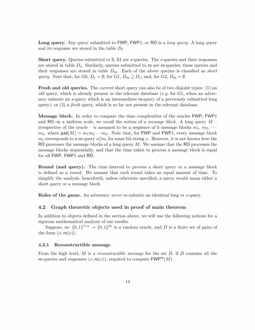
Long query. Any query submitted to FWP, FWP1, or RO is a long query. A long query and its response are stored in the table Dl.

Short query. Queries submitted to S, S1 are s-queries. The s-queries and their responses are stored in table Ds. Similarly, queries submitted to ro are ro-queries; these queries and their responses are stored in table Dro. Each of the above queries is classified as short query. Note that, for G0, Ds = ∅; for G1, Dro ⊇ Ds; and, for G2, Dro = ∅.

Fresh and old queries. The current short query can also be of two disjoint types: (1) an old query, which is already present in the relevant database (e.g. for G1, when an adversary submits an s-query which is an intermediate ro-query of a previously submitted long query); or (2) a fresh query, which is so far not present in the relevant database.

Message block. In order to compare the time complexities of the oracles FWP, FWP1 and RO on a uniform scale, we recall the notion of a message block. A long query M – irrespective of the oracle – is assumed to be a sequence of k message blocks m1, m2, · · · mk, where pad(M) = m1m2 · · · mk. Note that, for FWP and FWP1, every message block mi corresponds to a ro-query x||mi for some bit-string x. However, it is not known how the RO processes the message blocks of a long query M . We assume that the RO processes the message blocks sequentially, and that the time taken to process a message block is equal for all FWP, FWP1 and RO.

Round (and query). The time interval to process a short query or a message block is defined as a round. We assume that each round takes an equal amount of time. To simplify the analysis, henceforth, unless otherwise specified, a query would mean either a short query or a message block.

Rules of the game. An adversary never re-submits an identical long or s-query.

4.2 Graph theoretic objects used in proof of main theorem

In addition to objects defined in the section above, we will use the following notions for a rigorous mathematical analysis of our results.

Suppose, ro : {0, 1}1+n → {0, 1}2n is a random oracle, and D is a finite set of pairs of the form (x, ro(x)).

4.2.1 Reconstructible message

From the high level, M is a reconstructible message for the set D, if D contains all the ro-queries and responses (x, ro(x)), required to compute FWPro(M).

14

' ' ' '

' '' ' ' '

''

' ' ' '

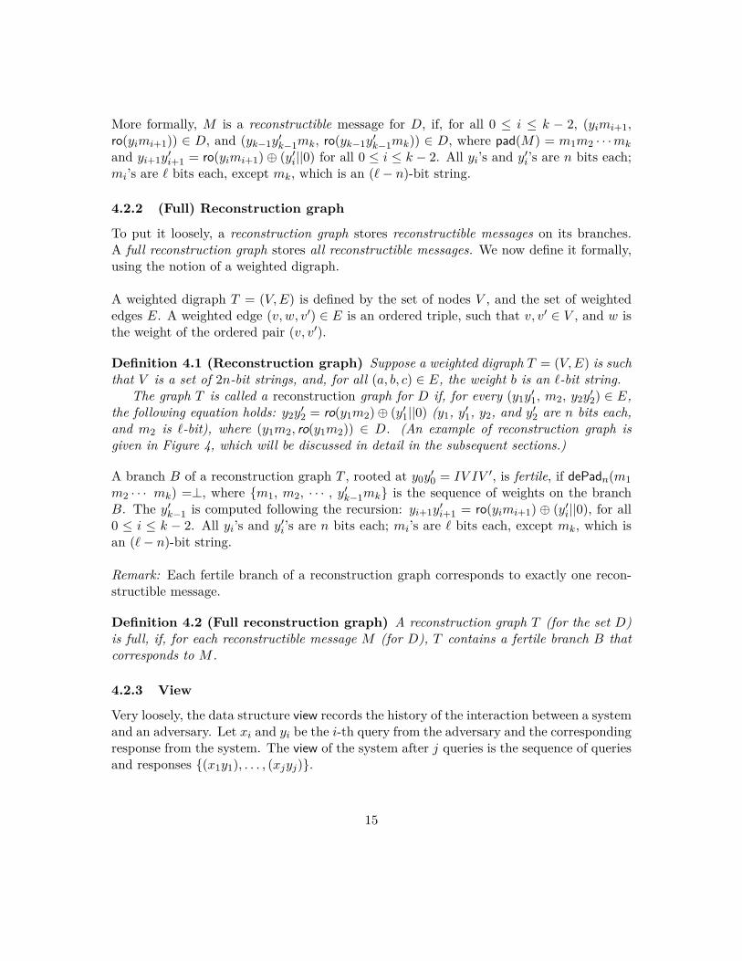
More formally, M is a reconstructible message for D, if, for all 0 ≤ i ≤ k − 2, (yimi+1, ro(yimi+1)) ∈ D, and (yk−1y k−1mk)) ∈ D, where pad(M) = m1m2 ·

i||0) for all 0 ≤ i ≤ k − 2.i+1 mi’s are . bits each, except mk, which is an (. − n)-bit string.

4.2.2 (Full) Reconstruction graph

To put it loosely, a reconstruction graph stores reconstructible messages on its branches. A full reconstruction graph stores all reconstructible messages. We now define it formally, using the notion of a weighted digraph.

A weighted digraph T = (V, E) is defined by the set of nodes V , and the set of weighted edges E. A weighted edge (v, w, v') ∈ E is an ordered triple, such that v, v' ∈ V , and w is the weight of the ordered pair (v, v').

'

Definition 4.1 (Reconstruction graph) Suppose a weighted digraph = ( ) is such T V, Ethat V is a set of 2n-bit strings, and, for all (a, b, c) ∈ E, the weight b is an .-bit string.

k−1mk, ro(yk−1y= ro(yimi+1) ⊕ (y

· · mk

and yi+1y All yi’s and y ’s are n bits each; i

1, m2, y2y2) ∈ E, 1||0) (y1, y1, y2, and y2 are n bits each, 2

and m2 is .-bit), where (y1m2, ro(y1m2)) ∈ D. (An example of reconstruction graph is given in Figure 4, which will be discussed in detail in the subsequent sections.)

The graph T is called a reconstruction graph for D if, for every (y1ythe following equation holds: y2y = ro(y1m2) ⊕ (y

A branch B of a reconstruction graph T , rooted at y0y = IV IV ', is fertile, if dePadn(m10 =⊥, where {m1, m2,

k−1 is computed following the recursion: yi+1ymk) k−1mk} is the sequence of weights on the branch

= ro(yimi+1) ⊕ (yi||0), for all i+1

m2 · · · · · · , yThe yB.

0 ≤ i ≤ k − 2. All yi’s and yi’s are n bits each; mi’s are . bits each, except mk, which is an (. − n)-bit string.

Remark: Each fertile branch of a reconstruction graph corresponds to exactly one reconstructible message.

Definition 4.2 (Full reconstruction graph) A reconstruction graph T (for the set D) is full, if, for each reconstructible message M (for D), T contains a fertile branch B that corresponds to M .

4.2.3 View

Very loosely, the data structure view records the history of the interaction between a system and an adversary. Let xi and yi be the i-th query from the adversary and the corresponding response from the system. The view of the system after j queries is the sequence of queries and responses {(x1y1), . . . , (xjyj )}.

15

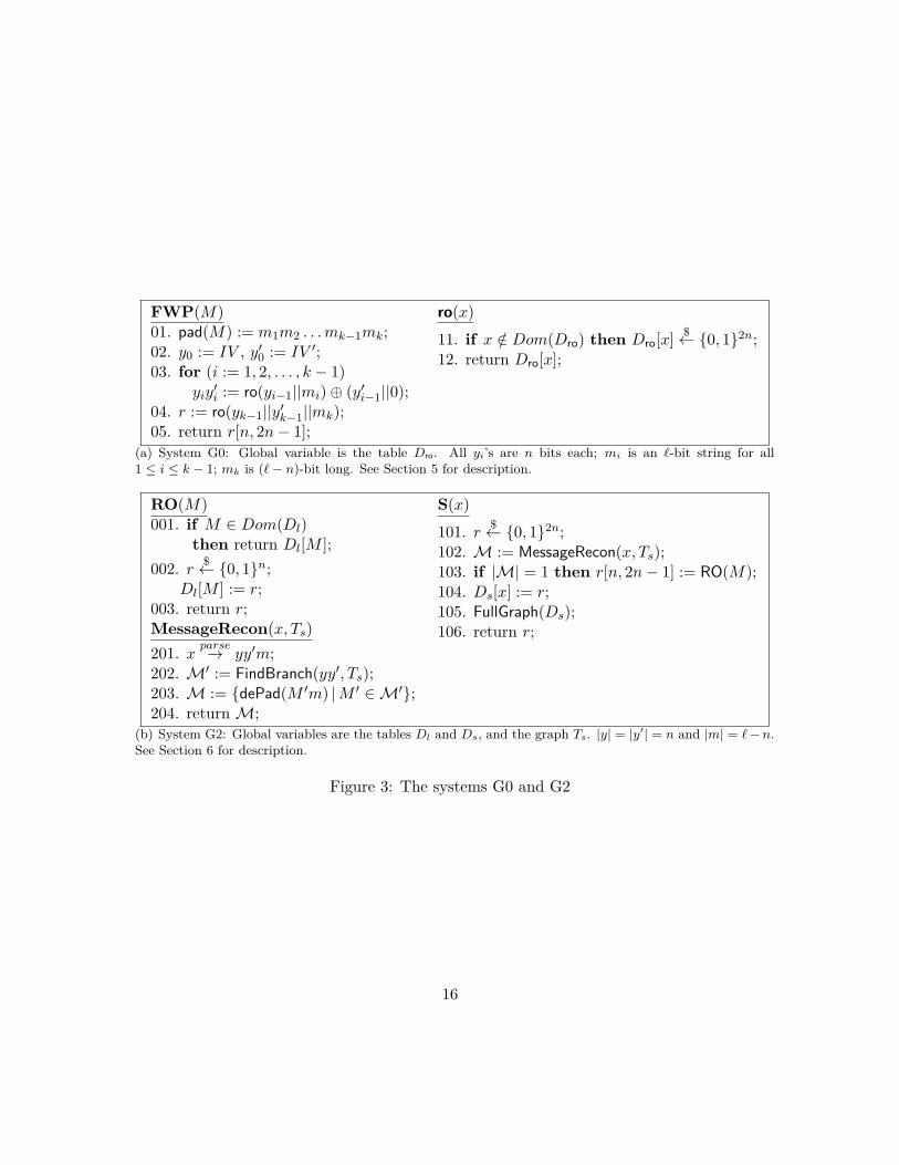
FWP(M) ro(x) 01. pad(M) := m1m2 . . . mk−1mk; $11. if x /∈ Dom(Dro) then Dro[x] ← {0, 1}2n;'02. y0 := IV , y0 := IV '; 12. return Dro[x];03. for (i := 1, 2, . . . , k − 1)

yiy' := ro(yi−1||mi) ⊕ (yi

'−1||0);i

'04. r := ro(yk−1||yk−1||mk); 05. return r[n, 2n − 1];

(a) System G0: Global variable is the table Dro. All yi’s are n bits each; mi is an f-bit string for all 1 ≤ i ≤ k − 1; mk is (f − n)-bit long. See Section 5 for description.

RO(M) S(x) 001. if M ∈ Dom(Dl) $101. r ← {0, 1}2n;

then return Dl[M ]; $

102. M := MessageRecon(x, Ts); 002. r ← {0, 1}n; 103. if |M| = 1 then r[n, 2n − 1] := RO(M);

Dl[M ] := r; 104. Ds[x] := r; 003. return r; 105. FullGraph(Ds); MessageRecon(x, Ts) 106. return r;

parse '201. x → yy m; 202. M' := FindBranch(yy', Ts); 203. M := {dePad(M 'm) | M ' ∈M'}; 204. return M;

(b) System G2: Global variables are the tables Dl and Ds, and the graph Ts. |y| = |y1| = n and |m| = f − n. See Section 6 for description.

Figure 3: The systems G0 and G2

16

5 Main system G0

Following the definition in Section 2.2, the system G0 implements the FWP mode using the random oracle ro : {0, 1}1+n → {0, 1}2n (see Figure 3(a)).

6 Main system G2

See Figure 3(b) for the pseudocode. The random oracle RO mentioned in Section 3 is implemented through lazy sampling. The only remaining part is to construct the simulator S. Our design strategy for the simulator is fairly straightforward and simple. Before going into the details, we first provide a high level intuition.

6.1 Intuition for simulator S

The purpose of the simulator pair S is two-pronged: (1) to output values that are indistinguishable from the output from the random oracle ro, and (2) to respond in such a way that FWPro(M) and RO(M) are identically distributed. It will easily follow that as long as the simulator S is able to output values satisfying the above conditions, no adversary can distinguish between G0 and G2.

To achieve (1), the simulator S, for a distinct input x, should output a random value, such that the distributions of S(x) and ro(x) are close.

To achieve (2), the simulator needs to do the following:

• Building the full reconstruction graph. To asses the adversarial power, the simulator S maintains the full reconstruction graph Ts for the set Ds containing all s-queries and responses; this helps the simulator keep track of all ‘FWP-mode-compatible’ messages (more formally, all reconstructible messages) that can be formed using the ‘known’ information. This is accomplished by a special subroutine FullGraph. The pictorial representation of the reconstruction graph Ts is given in Figure 4.

• Adjusting the elements of the tables Dl and Ds. Whenever a new reconstructible message M is found using the aforementioned reconstruction graph Ts, the simulator makes this crucial adjustment: it assigns FWPS(M) := RO(M). It is fairly intuitive that, if S and ro produce outputs according to statistically close distributions, then the distributions of FWPS(M) and FWPro(M) are also close. Since FWPS(M) = RO(M), the distributions of RO(M) and FWPro(M) are also close. This is accomplished by the subroutine MessageRecon.

17

6.2 Detailed description of simulator S

We first describe the two most important parts of the simulator S: the subroutines Full-Graph and MessageRecon. See Figure 3(b) for the pseudocode.

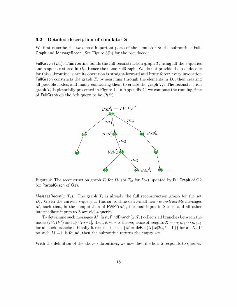
FullGraph (Ds): This routine builds the full reconstruction graph Ts using all the s-queries and responses stored in Ds. Hence the name FullGraph. We do not provide the pseudocode for this subroutine, since its operation is straight-forward and brute force: every invocation FullGraph constructs the graph Ts by searching through the elements in Ds, then creating all possible nodes, and finally connecting them to create the graph Ts. The reconstruction graph Ts is pictorially presented in Figure 4. In Appendix C, we compute the running time of FullGraph on the i-th query to be O(i4).

y0y′0 = IV IV ′

m1ma

m2

m3

yay′ay1y

′1

y2y′2

y3y′3

Figure 4: The reconstruction graph Ts for Ds (or Tro for Dro) updated by FullGraph of G2 (or PartialGraph of G1).

MessageRecon(x, Ts). The graph Ts is already the full reconstruction graph for the set Ds. Given the current s-query x, this subroutine derives all new reconstructible messages M , such that, in the computation of FWPS(M), the final input to S is x, and all other intermediate inputs to S are old s-queries.

To determine such messages M , first, FindBranch(x, Ts) collects all branches between the nodes (IV, IV ') and x[0, 2n−1]; then, it selects the sequence of weights X = m1m2 · · · mk−1

for all such branches. Finally it returns the set {M = dePad(X||x[2n, . − 1])} for all X. If no such M =⊥ is found, then the subroutine returns the empty set.

With the definition of the above subroutines, we now describe how S responds to queries.

18

An s-query and response: For an s-query, the simulator S assigns a uniformly sampled 2n-bit value to r. Then the subroutine MessageRecon(x, Ts) is invoked that returns a set of reconstructible messages M. If |M| = 1 then the RO is invoked on M ∈ M, and the value is assigned to r[n, 2n − 1]. Finally, the graph Ts is updated by FullGraph, before r is returned. In Appendix C, we show that the worst-case running time of S after σ queries is O(σ5).

7 Intermediate system G1

For description see Figure 5. For the sake of clear understanding, we first discuss the motivation for designing this system.

7.1 Motivation

The main motivation for constructing a new system G1 is that it is difficult to compare between the executions of the systems G0 and G2, instruction by instruction. The difficulty arises from the fact that G2 has a graph Ts, and two extra subroutines FullGraph, and MessageRecon, while G0 has no such graphs or subroutines. To get around this difficulty, we reduce G0 to an equivalent system G1 by endowing it with additional memory for constructing the graph Tro, and by supplying it with additional subroutines MessageRecon and PartialGraph. These additional components do not result in any difference in the input and output distributions of the systems G0 and G1 for any adversary (this result is formalized in Proposition 8.1); therefore, in the indifferentiability framework, G0 can be replaced by G1.

Even though G1 and G2 now appear ‘similar’, there are still important differences. The most crucial of them is that, in the former case, the long queries are processed as a sequence of ro-queries; therefore, current s-queries of G1 may match old ro-queries and responses, while such events are not possible for G2. This difference comes with two implications:

1. The reconstruction graph Tro in G1 is built using s-queries, ro-queries and their responses stored in the table Dro; in case of G2, the reconstruction graph Ts is built using only s-queries and responses stored in Ds. We extract from Tro the maximally connected subgraph built from all the s-queries and responses stored in Ds; we call the subgraph Ts. Now the reconstruction graph Ts in both systems are comparable, since they are both built from the set Ds.

2. In G1, the reconstruction graph Tro may not be full for the set Dro, since the subroutine PartialGraph adds only a few nodes – rather than all nodes – to Tro every round; by contrast, the reconstruction graph Ts – built by the subroutine FullGraph – for G2 is necessarily full for the set Ds. In Section 9, we identify a set of events in the system G1, and then, in Section 10, show that, if those events do not occur, then the reconstruction graphs in both the systems are full.

19

7.2 Detailed description of G1

Figure 5: System G1: Global variables are the tables Dl and Dro (Ds is contained in Dro), and the graph Tro (Ts is a connected subgraph of Tro). See Section 7 for description.

FWP1(M) S1(x)

001. pad(M) := m1m2 · · · mk−1mk; 100. if Type2 then BAD :=True ; '002. y0 := IV , y0 := IV '; 101. r := ro(x);

003. for (i := 1, · · · , k − 1){ 102. M := MessageRecon(x, Ts); 004. r := ro(yi−1mi); 103. if |M| = 1 ∧ M /∈ Dom(Dl) then

' '005. yiy := r ⊕ (yi−1||0); Dl[M ] := r[n, 2n − 1];i 006. if yi−1mi is fresh then 104. Ds[x] := r;

PartialGraph(yi−1mi, r, Tro);} 105. if x is fresh then PartialGraph(x, r, Tro); BAD := True ; 106. return r;007. if Type3 then

'008. r := ro(yk−1yk−1mk); '009. if yk−1yk−1mk is fresh then PartialGraph(x, r, Tro)

' parse parsePartialGraph(yk−1yk−1mk, r, Tro); 400. x → ycm; r → y ∗ y '; 010. Dl[M ] := r[n, 2n − 1]; 401. if Type0 then BAD := True ; 011. return r[n, 2n − 1]; 402. C := ContactPoints(yc);

/*1st Phase: (403 – 405)*/ 'MessageRecon(x, Ts) 403. E := {(ycy , m, yy ')|c

parse ' ''201. x → yy m; y := y ∗ ⊕ y , ycy ∈ C};c c

202. M ' := FindBranch(yy ' , Ts); 404. for e ∈ E {AddEdge(e); ' '203. M := {dePad(M m) | M ∈M ' }; 405. if Type1-a ∨ Type1-b ∨ Type1-c then

BAD := True ;} /*2nd Phase: (406 – 413)*/

ro(x) 406. for (x, r) ∈ Dro

204. return M;

'301. if x /∈ Dom(Dro) 407. for(ycyc, m, yy ') ∈ E

then Dro[x] ← {0, 1}2n; 408. if y = x[0, n − 1] then$

409. {z := r[0, n − 1] ⊕ y ';302. return Dro[x]; '410. z := r[n, 2n − 1]; '411. m := x[n, n + . − 1];

' '412. AddEdge(yy , m , zz '); 413. if Type1-d ∨ Type1-e ∨ Type1-f then

BAD := True ;}

In our first description of this system, we will ignore the statements where the variable BAD is set, since they impact neither the output nor the global data structures. The variable BAD is set when certain events occur in the global data structures. Those events will be discussed in Section 9. We now describe the subroutines used by this system.

20

PartialGraph(x, r, Tro): This subroutine is called only when a fresh ro-query is produced. This subroutine updates the reconstruction graph Tro (for the set Dro) in the following way: Rather than building all possible paths using elements of Dro, this routine augments the Tro in at most two phases; hence the name PartialGraph. The details are as follows. First, the subroutine ContactPoints(yc = x[0, n − 1]) is invoked, which returns a set C containing all nodes in Tro, whose least-significant n bits are x[0, n − 1]. We note that the nodes of Tro contained in C are the places where the fresh ro-query will be attached. The pictorial representation of Tro is in Figure 4.

1st phase: Using the members of the set C and the fresh query-response pair (x, r), fresh edges are constructed, stored in the set E, and then added to Tro using the subroutine AddEdge.

2nd phase: In this phase, a 2nd set of fresh nodes are added to the fresh nodes of the 1st phase, using all query-response pairs stored in table Dro. The details are as follows: if the least significant n bits of an old query x ∈ Dom(Dro) equals the least significant n bits of the tail node of an edge e ∈ EdgeNew, then a fresh edge is constructed as before, and then it is attached to the tail node of e using AddEdge.

MessageRecon(x, Ts). This subroutine has already been described in the context of G2. However, in this context of G1, there is an important point to note: The graph Ts used by this subroutine is the maximally connected subgraph of Tro generated by the s-queries and responses with root (IV, IV ').

Now we describe how the oracles FWP1 and S1 respond to queries.

FWP1: FWP1 mimics FWP, while updating the graph Tro using the subroutine Partial-Graph, whenever a fresh ro-query is generated. Dl[M ] is assigned r[n, 2n − 1], where r is the output from the final ro call. Finally, r[n, 2n − 1] is returned.

Simulator S1: Given the s-query x, the s-oracle S1 computes ro(x) = r. Then the subroutine MessageRecon(x, Ts) is called which returns a set of messages M. If |M| = 1, and if M /∈ Dl[M ], then Dl[M ] is assigned the value of r[n, 2n−1]. Before finally returning r[n, 2n − 1], the subroutine PartialGraph is called with input (x, r, Tro), if it is fresh, to update the existing graph Tro.

21

8 First Part of Main Theorem: Proof of (2) With the description of the systems (in Sections 5, 6, and 7) at our disposal, we are well equipped to prove (2).

Proposition 8.1 For any distinguishing adversary A,

Pr AG0 ⇒ 1 = Pr AG1 ⇒ 1 .

Proof. From the description of S1, we observe that, for all x ∈ {0, 1}1+n, S1(x) = ro(x). Likewise, from the description of FWP1 and FWP, for all M ∈ {0, 1}∗ , FWP1(M) = FWP(M). �

9 Type0, 1, 2, and 3, of System G1

In this section, we concretely define the Type0, Type1, Type2, and Type3 events of the system G1 (see Figure 5). Informally they will be called ‘bad’ events, since these events set the variable BAD in G1. We first provide the motivation for these events.

9.1 Motivation

We recall that the adversary submits s- and long queries to the system G1 and receives responses, and based on the history of query-response pairs – known as view – she then tries to distinguish G1 from G2. Intuitively, those events are called ‘bad’, for which the outputs from the ro oracles of G1 can be predicted by the adversary with probability better than when interacting with G2. These events primarily involve various forms of collision occurring in the outputs of queries, allowing the adversary to generate non-trivial reconstructible messages. Secondly, we need to catch the events where current queries match old queries too. One can intuit that these events may help the adversary in distinguishing G1 from G2. It is also important to note that, if Tro is not a full reconstruction graph then the adversary can also use this fact to compel G1 to produce outputs different from those from G2 (since G2 always maintains the full reconstruction graph Ts). Lastly, the absence of ‘bad’ events will be able to restrict the growth of the reconstruction graph Tro every round; this limits the number of reconstructible messages.

Next sections deal with concrete definitions of these events, keeping the above motivation in mind.

9.2 Classifying elements of Dro, branches of Tro, and ro-queries

Definition of Type0 to Type3 events depend on the elements in Dro, the branches of Tro, and the types of ro-queries. In the following sections we first classify them.

22

Q1 Q2 Q3 Q4 Q5 Q6

(i)

Q1 Q2

(ii)

==

Current

x

r

(iv)

==

Current

x

rQ5Q3 Q4

==

Current

x

r(iii)

LegendsRed and green objects are

unknown and known to theadversary

Input and output for oracle

ro; Head node, and tail

node denote (n, n, l − n)-bit

input, and (n, n)-bit output

Current

New inputs and outputsfor oracle ro; all arrowsare n bits each, exceptfor the bold arrowwhich is l − n bits

U [0, 22n − 1]�

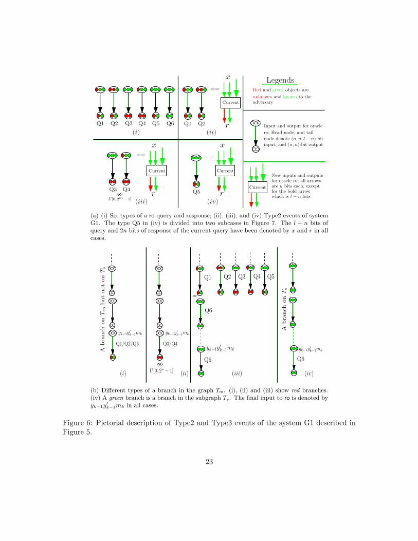
(a) (i) Six types of a ro-query and response; (ii), (iii), and (iv) Type2 events of system G1. The type Q5 in (iv) is divided into two subcases in Figure 7. The l + n bits of query and 2n bits of response of the current query have been denoted by x and r in all cases.

Q1

Q6

=

Q6

Q2 Q3 Q4 Q5

yk−1y′k−1mk

Q6

yk−1y′k−1mk

Abranch

onTs

(iii) (iv)

Abranch

onTrobutnotonTs

(i) (ii)

Q1/Q2/Q5

yk−1y′k−1mk

Q3/Q4

yk−1y′k−1mk

�U [0, 2n − 1]

(b) Different types of a branch in the graph Tro. (i), (ii) and (iii) show red branches. (iv) A green branch is a branch in the subgraph Ts. The final input to ro is denoted by yk−1yk

1−1mk in all cases.

Figure 6: Pictorial description of Type2 and Type3 events of the system G1 described in Figure 5.

23

Q6

Q6

Q6

Q5Current

x

r

===

�U [0, 2n − 1]

Type Q5-1

IV IV ′

Apa

thon

T rorepresenting

along

query

IV IV ′

Q1

Q6

=

Q6

Q5Current

x

r

===

Type Q5-2

Q2 Q3 Q4 Q5

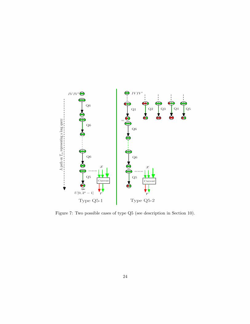
Figure 7: Two possible cases of type Q5 (see description in Section 10).

24

9.2.1 Elements of Dro: six types

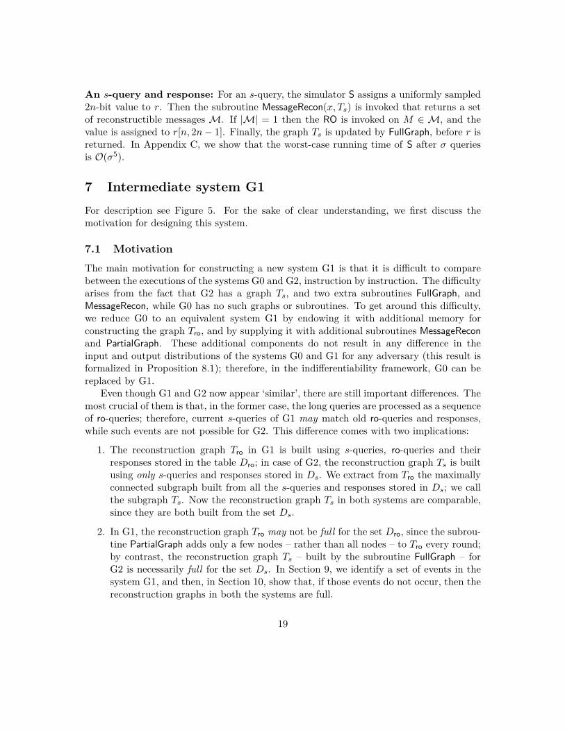
We deal with an event when the current s-query x is already in the table Dro. We classify the elements stored in Dro, according to its known and unknown parts. The known part of a ro-query and response is the part that is present in the view of the system G1, or it can be derived from the view with probability 1; the unknown part is not present in the view, and it cannot be derived from the view with probability 1. There are six types of an old query-response denoted by Q1, Q2, Q3, Q4, Q5 and Q6, as shown in Figure 6(a)(i). See Appendix D for the proof. The first five types were generated as the intermediate ro-queries and responses during the execution of old long queries; the sixth type is an old s-query and the response. The red and green circles denote the unknown and the known parts. The higher order bits are placed on the right. We divide a Q5 query into two cases according to its position in Tro (depicted in Figure 7): (Q5-1) In a branch, all ro-queries preceding the Q5 query are of type Q6; (Q5-2) In a branch, there is at least one ro-query (preceding the Q5 query) which is not of type Q6.

9.2.2 Branches of Tro: four types

The branches of Tro can be classified into four types, as shown in Figure 6(b)(i) to (iv). A branch B is: type (i), if the final query is Q1, Q2 or Q5; type (ii), if the final query is Q3 or Q4; type (iii), if the final query is Q6, and if one of the intermediate queries is Q1, Q2, Q3, Q4 or Q5; type (iv), if all queries are Q6. The first three types are called red branch. The fourth type is called green branch.

9.2.3 The ro-queries: seven types

We observe that – based on the types described in the sections above – the current ro-query can be categorized into the following classes.

1. Current ro-query is an s-query. This can be of two types.

(a) The ro-query is fresh. (b) The ro-query is one of six types of elements in Dro described in Section 9.2.1.

2. Current ro-query is an intermediate ro-query for the current long query. This is of three types.

(a) Current long query is present on a red branch – as defined in Section 9.2.2 – of the graph Tro. The ro-query in this case is necessarily one of six types stored in Dro; we divide it into two cases.

i. The ro-query is the final one. ii. The ro-query is a non-final one.

25

(b) Current long query is present on a green branch of the graph Tro. The ro-query in this case is also one of six types stored in Dro.

(c) Current long query is not present on a branch of the graph Tro. We divide the ro-query into two types.

i. The ro-query is fresh. ii. The ro-query is one of six types of elements in Dro.

9.3 Definition: Type0 and Type1 on fresh queries

9.3.1 Intuition

We address the classes 1a, and 2c(i) of Section 9.2.3 together, since they are connected by the fact that the ro-query is fresh. As described in Section 9.1, for a fresh query, the absence of ‘bad’ events (1) prevents generation of nontrivial reconstructible messages, (2) (linearly) restricts the growth of the graph Tro, and (3) makes Tro a full reconstruction graph.

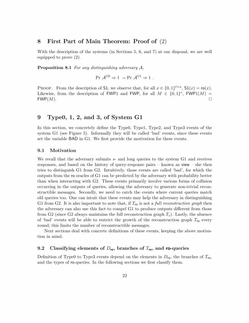
1. A non-trivial reconstructible message is generated, (i) if the fresh ro-query causes a node collision in the graph Tro, or (ii) if it causes an old query to be attached to a fresh node. Type1-a, Type1-c, Type1-d and Type1-f events cover all the above conditions. See Figure 8(b).

2. Absence of Type0, Type1-b, and Type1-d restricts the growth of the graph Tro to a constant number of nodes every fresh query (i.e., linearly after σ fresh queries). See Figures 8(a) and 8(b).

3. The goal of Type1-f – in addition to the one described in (1) – is that its absence makes Tro a full reconstruction graph after two phases.

Importance of the two-phase framework: The first novelty of our work lies in our carefully designed ‘bad’ events – especially the Type0 and Type1 events – that are spread across two phases. More precisely, the absence of these events allows the graph Tro to be augmented in two phases, rather than in one phase (see Figure 8); at the same time, it allows the graph to have the aforementioned properties. The two-phase framework – as we will see subsequently – is essential in breaking the birthday barrier of n/2 bits. In a similar way, the two-phase framework could be extended to a three-phase framework to go even beyond 2n/3 bits (see Section 13). But a rigorous theoretical analysis of that is a challenging task.

26

Fresh Old1 Old2

yc m

y∗y′

= =

3-multi-collision on right coordinates

(a) Type0 event of system G1.

Type1-a Type1-b Type1-c

Node-collision 3-multi-collision on left coordinatesQuery collision

(2n bits)

1stphase

2ndphase

Notation

Fresh

yc y′c

m

y y′

y∗

Old

==

Fresh

yc y′c

m

yy′

y∗

Old1

=

Old2

=

Fresh

yc y′c m

y y′

y∗

==

Old

Fresh

yc y′c m

y

y∗

Type1-d

y′

Old1 Old2

m′

z z′==E2

=E1

Node collision 3-multi-collision on left coordinates

Fresh

yc y′c m

y

y∗

Type1-e

y′

Old1 Old2

m′

zz′ =

E2

=E1

Old3

=E2

Query collision(n bits)

Type1-f

Fresh

yc y′c m

y

y∗

y′

Old1

m′

zz′ =

E2

=E1

Old2

random n bits n bits l − n bits l bits

= event of n bit equality == event of 2n bit equality

(b) Type1-a,b,c,d,e,f events of system G1.

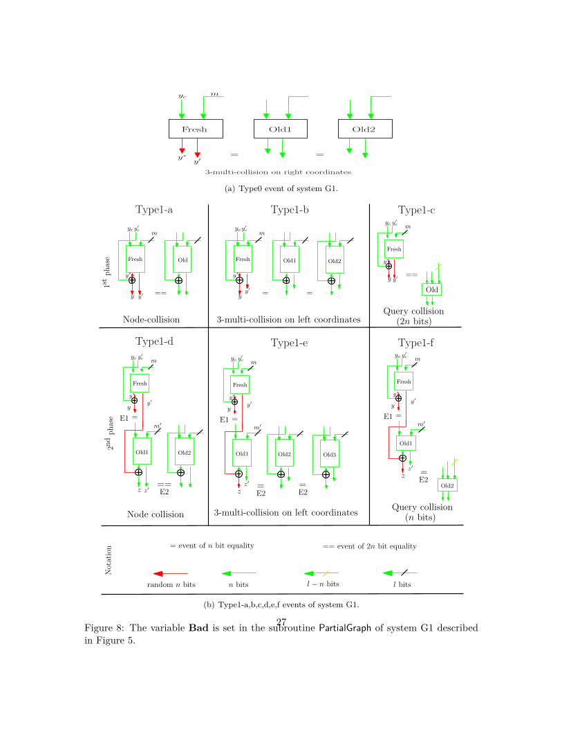
27Figure 8: The variable Bad is set in the subroutine PartialGraph of system G1 described in Figure 5.

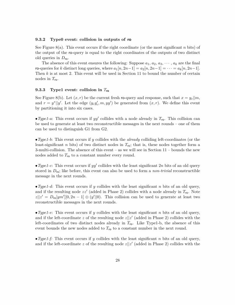
9.3.2 Type0 event: collision in outputs of ro

See Figure 8(a). This event occurs if the right coordinate (or the most significant n bits) of the output of the ro-query is equal to the right coordinates of the outputs of two distinct old queries in Dro.

The absence of this event ensures the following: Suppose a1, a2, a3, · · · , ak are the final ro-queries for k distinct long queries, where a1[n, 2n−1] = a2[n, 2n−1] = · · · = ak[n, 2n−1]. Then k is at most 2. This event will be used in Section 11 to bound the number of certain nodes in Tro.

9.3.3 Type1 event: collision in Tro

See Figure 8(b). Let (x, r) be the current fresh ro-query and response, such that x = yc||m, ' 'and r = y ∗||y . Let the edge (ycy , m, yy ') be generated from (x, r). We define this event c

by partitioning it into six cases.

' •Type1-a: This event occurs if yy collides with a node already in Tro. This collision can be used to generate at least two reconstructible messages in the next rounds – one of them can be used to distinguish G1 from G2.

•Type1-b: This event occurs if y collides with the already colliding left-coordinates (or the least-significant n bits) of two distinct nodes in Tro; that is, these nodes together form a 3-multi-collision. The absence of this event – as we will see in Section 11 – bounds the new nodes added to Tro to a constant number every round.

' •Type1-c: This event occurs if yy collides with the least significant 2n bits of an old query stored in Dro; like before, this event can also be used to form a non-trivial reconstructible message in the next rounds.

•Type1-d: This event occurs if y collides with the least significant n bits of an old query, 'and if the resulting node zz (added in Phase 2) collides with a node already in Tro. Note

' z||z = Dro[ym '][0, 2n − 1] ⊕ (y ' ||0). This collision can be used to generate at least two reconstructible messages in the next rounds.

•Type1-e: This event occurs if y collides with the least significant n bits of an old query, 'and if the left-coordinate z of the resulting node z||z (added in Phase 2) collides with the

left-coordinates of two distinct nodes already in Tro. Like Type1-b, the absence of this event bounds the new nodes added to Tro to a constant number in the next round.

•Type1-f: This event occurs if y collides with the least significant n bits of an old query, 'and if the left-coordinate z of the resulting node z||z (added in Phase 2) collides with the

28

least significant n bits of an old query. The absence of this event serves two goals at the same time: (1) it rules out the generation of a non-trivial reconstructible message and (2) it restricts the growth of Tro only up to two phases every round.

9.4 Type2 and Type3 on old queries

9.4.1 Intuition

Now we deal with the classes 1b, 2a, 2b and 2c(ii) of Section 9.2.3. All of them address the issue when the current queries match old ones.

The class 1b happens, when an s-query matches one of five types of old elements stored in Dro; these events can potentially help the adversary in distinguishing between G1 and G2, and we identify class 1b as Type2, and class 2a as Type3 events; the case by case analysis of the events will follow in a while.

The remaining classes are now 2a, 2b and 2c(ii), when the adversary submits a long query – say M – to the oracle FWP1, and it is found that M is already present on some (fertile) branch of the graph Tro (2a and 2b), or it is not present at all on any branch of Tro (2c(ii)). The class 2c(ii) necessarily includes a fresh ro-query followed possibly by old ro-queries, and this scenario has already been considered in various forms of Type1 events.

It is clear that the class 2a(ii) and 2b will not help the adversary in distinguishing G1 from G2.

So now we focus on the class 2a(i), which deals with the final ro-query of a red branch. Depending on the type of branch, the adversary tries to predict the most significant n bits of the final ro-query (i.e., the hash output) with non-trivial probability; she succeeds only for Type3 events that will be discussed shortly.

9.4.2 Type2

Recall that a query-response pair in Dro can be of six types: Q1 to Q6. Type2 event is divided into several cases depending on the type of the current s-query. See Figure 6(a)(iiiv) for the pictorial presentation. Suppose (x, r) is the input-output of a fresh query.

Type2-a: If the query is of type Q1.

Type2-b: If the query is of type Q2.

Type2-c: If the query is of type Q5-2.

Type2-d: If the query is of type Q3, and if r is distinguishable from the uniform distribution U [0, 22n − 1].

29

Type2-e: If the query is of type Q4, and if r is distinguishable from the uniform distribution U [0, 22n − 1].

Type2-f: If the query is of type Q5-1, and if r[0, n − 1] is distinguishable from the uniform distribution U [0, 2n − 1].

9.4.3 Type3

In this case, we consider the final ro-query of a red branch as the current query. Several types of red branch – (i), (ii), and (iii) – are shown in Figure 6(b).

There are three types of Type3 event:

Type3-a If the current long query M is present as a red branch of type (i).3

Type3-b If the current long query M is present as a red branch of type (ii), and if the most significant n bits of output being distinguishable from the uniform distribution U [0, 2n −1].

Type3-c If the current long query M is present as a red branch of type (iii).

10 Second Part of Main Theorem: Proof of (3) First, we first fix a few definitions.

10.1 Definitions: GOODi and BADi

Events GOODi and BADi. BADi denotes the event when the variable BAD is set during round i of G1, that is, when Type0, Type 1, Type2, or Type3 events occur. Let the sympibol GOODi denote the event ¬ j=1 BADi. The symbol GOOD0 denotes the event when no queries are submitted. From a high level, the intuition behind the construction of the BADi event is straight-forward: we will show that if BADi does not occur, and if GOODi−1

did occur, then the views of G1 and G2 (after i rounds) are identically distributed for any attacker A.

Events GOOD1i and BAD1i. In order to get around a small technical difficulty in establishing the uniform probability distribution of certain random variables, we need to modify the above events GOODi and BADi slightly. The event BAD1i occurs when Type0, Type2, or Type3 events occur in the i-th round. The event GOOD1i is defined as GOODi−1 ∧¬BAD1i.

13Observe that this case implies a node-collision in Tro, since the yk−1yk−1mk is the final ro-query for two distinct l-queries, the current M and also an old one. Therefore, if Type1 event did not occur in the previous rounds, this event is impossible in the current round.

30

10.2 Proof of (3)

With the help of the Type0 to Type3 events described in Section 9, we are equipped to prove (3). Recall that we need to show two things:

Pr AG1 ⇒ 1 − Pr AG2 ⇒ 1 ≤ Pr ¬GOOD1σ (5)

as well as σ

Pr ¬GOOD1σ ≤ Pr ¬GOODσ ≤ Pr BADi | GOODi−1 . (6) i=1

Proof of (6) is straight-forward. To prove (5), we proceed in the following way. Observe

Pr AG1 ⇒ 1 − Pr AG2 ⇒ 1 = Pr AG1 ⇒ 1 | GOOD1σ − Pr AG2 ⇒ 1 | GOOD1σ · Pr GOOD1σ + Pr AG1 ⇒ 1 | ¬GOOD1σ − Pr AG2 ⇒ 1 | ¬GOOD1σ · Pr ¬GOOD1σ . (7)

If we can show that

Pr AG1 ⇒ 1 | GOOD1σ = Pr AG2 ⇒ 1 | GOOD1σ , (8)

then (7) reduces to (5), since

Pr AG1 ⇒ 1 | ¬GOOD1σ − Pr AG2 ⇒ 1 | ¬GOOD1σ ≤ 1.

As a result, we focus on establishing (8), which is done in Appendix E.

11 A Few Combinatorial Results

In order to prove (4), we will need a few combinatorial results. We first fix some notation.

Node(i): The multiset of nodes in Tro after i rounds in system G1.

(i) (i)N1 (and N2 ): The number of nodes added to Tro, during the 1st phase (and 2nd phase) of the i-th iteration of system G1.

(i)Dro : The table Dro after i rounds.

(i)Nright(a): The number of nodes in Tro after i rounds, where the most significant n bits equal a.

31

Left-CosetA(x): Suppose A is a multiset on {0, 1}2n. The multiset Left-CosetA(x) = {a ∈ A | a[0, n − 1] = x} contains all elements of A whose least significant n bits are equal to x. Such a sub-multiset will be called a left-coset of A, or simply a left-coset if A is clear from the context.

Right-CosetA(x): Suppose A is a multiset on {0, 1}2n. The multiset Right-CosetA(x) = {a ∈ A | a[n, 2n − 1] = x} contains all elements of A whose most-significant n bits equal x. As above, we will call such a sub-multiset a right-coset of A, or simply a right-coset.

twin-left/twin-right: A 2n-bit string a is a twin-left/twin-right of a 2n-bit string b, if a[0, n − 1] = b[0, n − 1]/if a[n, 2n − 1] = b[n, 2n − 1].

We now prove three important lemmas. The first one upper-bounds the size of the graph Tro, while the other two provide upper-bounds for the collision probability on the left and right coordinates of query-outputs and nodes on the graph.

(i)Lemma 11.1 (Node Counting) Given GOODi−1 occurs (i ≥ 1), then (i) N1 ≤ 2, (ii) (i) (i−1)

N ≤ i, (iii) Nright (a) ≤ 4 for all a ∈ {0, 1}n, and (iv) |Node(i−1)| ≤ 2i − 1.2

Proof. Since GOODi−1 occurred, the events Type0, Type1-b and Type1-e did not occur during the first i − 1 rounds of system G1. Therefore, the maximum size of the set Coset is 2 after i − 1 rounds.

(i)(i) N1 is upper-bounded by the maximum size of the set Coset after i − 1 rounds, from which the result follows.

(ii) In the second phase of the i-th round, a query cannot be added to more than 1 node of Tro, since the nodes generated during the first phase have distinct left-coordinates. As there are i queries, we get the result.

(iii) We note that, given GOODi−1 occurred – which essentially implies that Type0 (or 3-multi-collision on the most significant n bits of the output of a query), Type1-b and Type1-e (3-multi-collision on the least significant n bits of a node) did not occur – in the first i − 1 rounds. Therefore, one query can be placed in a maximum of 2 places on Tro, and at most two queries can have identical most significant n bits, implying the result.

(iv) We claim that the number of edges in Tro after i − 1 rounds is at most 2i − 2. Suppose there were more than 2i − 2 edges in Tro. This would require that we have at least one query which has been added to the graph at more than 2 nodes. However, this leads to a contradiction due to the fact that GOODi−1 occurred. Namely, we have that events

32

Type1-b and Type1-e did not occur. Now, since each edge has one tail node, including the root-node (IV, IV ') we get |Node(i−1)| ≤ 2i − 1. �

Since we assume σ

i=1 Pr BADi | GOODi−1 ≤ ε = 1/2 (see Section 3), (6) implies that GOODi ≥ 1/2 for all 0 ≤ i ≤ σ. In the following two lemmas we will use this fact.

Lemma 11.2 (Left Coordinate Collision) The following inequality holds:

2(|A| − 1)P i (y, A)

def Left-CosetA(y) ≥ 2 | GOODi−1 ∧ ∃yx ∈ A ≤ ,:= Prlcc 2n

where A ⊆ Node(i), and x ∈ {0, 1}n.

Proof. We now label the elements of A = {yj xj | j = 1, 2, · · · , k}. We choose any pair yj xj and yj1 xj1 from A, with j = j ' and note that

yj = ro(aj1 )[n, 2n − 1] ⊕ ro(aj2 )[0, n − 1], yj1 = ro(aj1 )[n, 2n − 1] ⊕ ro(aj1 )[0, n − 1].

1 2

We note that, if GOODi−1 occurs then aj1 ||aj2 = aj1 ||aj1 , implying 1 2

Pr yj = yj1 | GOODi−1 = Pr yj = yj1 | GOODi−1 ∧ aj1 ||aj2 = aj1 ||aj1

1 2 = Pr yj = yj1 | GOODi−1 ∧ aj1 ||aj2 = aj1 ||aj1 · Pr GOODi−1 | aj1 ||aj2 = aj1 ||aj1

1 2 1 2

1 · Pr GOODi−1 | aj1 ||aj2 = aj1 ||aj1

1 2 1= Pr yj = yj1 ∧ GOODi−1 | aj1 ||aj2 = aj1 ||aj1 · 1 2 Pr GOODi−1 | aj1 ||aj2 = aj1 ||aj1

1 2 1 ≤ Pr yj = yj1 | aj1 ||aj2 = aj1 ||aj1 · (9)1 2 Pr GOODi−1 | aj1 ||aj2 = aj1 ||aj1

1 2 Pr GOODi−1

Now, Pr GOODi−1 | aj1 ||aj2 = aj1 ||aj1 = since1 2 Pr aj1 ||aj2 �=aj1 ||aj1

1 2 Pr aj1 ||aj2 = aj1 ||aj1 | GOODi−1 = 1.

1 2

33

Putting this result in (9), we get,

Pr aj1 ||aj2 = aj1 ||aj1

Pr yj = yj1 | GOODi−1 ≤ 1 2 · Pr yj = yj1 | aj1 ||aj2 = aj1 ||aj1

Pr GOODi−1 1 2

1 ≤ · Pr yj = yj1 | aj1 ||aj2 = aj1 ||aj1 1 2Pr GOODi−1

1 1 = · Pr GOODi−1 2n

2 ≤ , since Pr GOODi−1 ≥ 1/2. (10)2n

Notice that P i (y, A) is essentially the probability that the multiset A contains at least lcc

one twin-left of the node yx ∈ A, given GOODi−1 occurred. Setting y1x1 = yx ∈ A, we get

P i (y, A) ≤ Pr i|A|

(y1 = yj ) | GOODi−1lccj=2

≤ |A|

Pr y1 = yj | GOODi−1 j=2

2(|A| − 1)= (using (10)). (11)2n

Thus the proof is complete. �

Lemma 11.3 (Right Coordinate Collision) The following inequality holds:

2(i − 2)P i (y, A)

def Right-CosetA(y) ≥ 2 | GOODi−1 ∧ ∃xy ∈ A ≤:= Pr ,rcc 2n

where the multiset A = {xj yj | j = 1, 2, · · · , i − 1} contains the outputs of previous i − 1 ro-queries, and x ∈ {0, 1}n.

Proof. We choose any pair xaya and xbyb from A, with a = b and note that

ya = ro(m)[n, 2n − 1], yb = ro(n)[n, 2n − 1],

where m and n are two previous ro-queries. Since m = n, 1Pr ya = yb | GOODi−1 ≤ · Pr ya = ybPr GOODi−1

2 ≤ , since Pr GOODi−1 ≥ 1/2. (12)2n

34

�

Notice that P i (y, A) is essentially the probability that the multiset A contains at least rcc

one twin-right of a node xy ∈ A, given GOODi−1 occurred. W.l.g, setting x1y1 = xy ∈ A, we get

ii−1

P i (y, A) ≤ Pr (y1 = yj ) | GOODi−1rccj=2

i−1

≤ Pr y1 = yj | GOODi−1 j=2

2(i − 2)≤ (by (12)).2n

12 Third (or Final) Part of Main Theorem: Proof of (4) To prove (4), we need individually compute the probabilities Type0i, Type1i, Type2i, and Type3i events described in Section 9. The suffix i denotes the corresponding event in the round i.

12.1 Estimating probability of Type0i

The Type0 event is displayed in Figure 8(a). The 2n-bit output of the ith ro-query – ∗ ' ∗ 'which is fresh – is denoted by yi yi. Let the multiset A = {yj y | j = 1, 2, · · · , i − 1}j

contain outputs of all previous i − 1 ro-queries. Now, from the definition of Type0 event we establish the following:

35

∗ ' 'Pr Type0i | GOODi−1 ≤ Pr ∃y yi ∈ A ∧ Right-CosetA(y ) ≥ 2 | GOODi−1i

∗ '= Pr ∃y yi ∈ A | GOODi−1

' ∗ ' · Pr Right-CosetA(y ) ≥ 2 | GOODi−1 ∧ ∃y yi ∈ Ai- ._ -Estimated in Lemma 11.3

ii−1 ' ' ' ≤ Pr (y = y ) | GOODi−1 · P i (yi, A)i j rcc

j=1

i−1 ' ' ' ≤ Pr y = yj | GOODi−1 ·P i (yi, A)i rcc

j=1 - ._ -1y independent of GOODi−1i

i−1 ' ' ' = Pr yi = yj · P i (yi, A)rcc

j=1

i − 1 2(i − 2)≤ · 2n 2n

2i2

≤ . (13)22n


(i) (i)We recall that if GOODi−1 occurs, then |Node(i−1)| = 2i − 1, N ≤ 2 and N ≤ i by 1 2 Lemma 11.1. Now, we can bound the probability of various Type1 events. The factor 2 on the left side of each inequality arises due to the two fresh nodes that can be added in the 1st phase. Several Type1 events are pictorially represented in Figure 8(b).

12.2.1 Computing probability of Type1-ai

Let N denote the number of nodes in the graph Tro after i− 1 full rounds and the 1st phase (i)of round i, given GOODi−1 occurred. Therefore, N = |Node(i−1)|+N ≤ 2i−1+2 = 2i+1.1

It is straight-forward to see from the figure,

N 2(2i + 1) 6iPr Type1-ai | GOODi−1 ≤ 2 · = ≤ . (14)22n 22n 22n

36

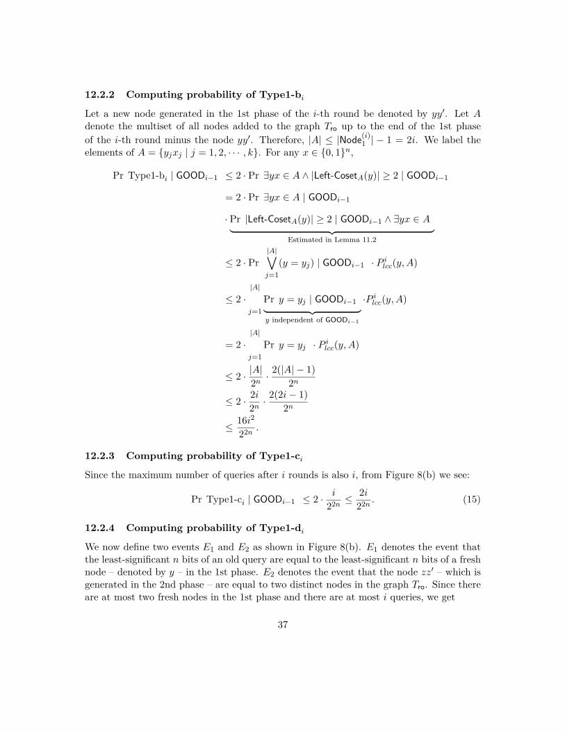
12.2.2 Computing probability of Type1-bi

'Let a new node generated in the 1st phase of the i-th round be denoted by yy . Let A denote the multiset of all nodes added to the graph Tro up to the end of the 1st phase

'of the i-th round minus the node yy . Therefore, |A| ≤ |Node(i)| − 1 = 2i. We label the 1 elements of A = {yj xj | j = 1, 2, · · · , k}. For any x ∈ {0, 1}n,

Pr Type1-bi | GOODi−1 ≤ 2 · Pr ∃yx ∈ A ∧ |Left-CosetA(y)| ≥ 2 | GOODi−1

= 2 · Pr ∃yx ∈ A | GOODi−1

· Pr |Left-CosetA(y)| ≥ 2 | GOODi−1 ∧ ∃yx ∈ A - ._ -Estimated in Lemma 11.2

≤ 2 · Pr |iA|

(y = yj ) | GOODi−1 · P i (y, A)lccj=1

≤ 2 · |A|

Pr y = yj | GOODi−1 ·P i (y, A)lccj=1 - ._ -

y independent of GOODi−1

|A|

= 2 · Pr y = yj · P i (y, A)lccj=1

|A| 2(|A| − 1)≤ 2 · · 2n 2n

2i 2(2i − 1)≤ 2 · · 2n 2n

16i2

≤ 22n .

12.2.3 Computing probability of Type1-ci

Since the maximum number of queries after i rounds is also i, from Figure 8(b) we see:

i 2iPr Type1-ci | GOODi−1 ≤ 2 · ≤ . (15)22n 22n

12.2.4 Computing probability of Type1-di

We now define two events E1 and E2 as shown in Figure 8(b). E1 denotes the event that the least-significant n bits of an old query are equal to the least-significant n bits of a fresh

'node – denoted by y – in the 1st phase. E2 denotes the event that the node zz – which is generated in the 2nd phase – are equal to two distinct nodes in the graph Tro. Since there are at most two fresh nodes in the 1st phase and there are at most i queries, we get

37

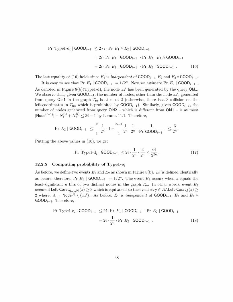
Pr Type1-di | GOODi−1 ≤ 2 · i · Pr E1 ∧ E2 | GOODi−1

= 2i · Pr E1 | GOODi−1 · Pr E2 | E1 ∧ GOODi−1

= 2i · Pr E1 | GOODi−1 · Pr E2 | GOODi−1 . (16)

The last equality of (16) holds since E1 is independent of GOODi−1, E2 and E2 ∧GOODi−1. It is easy to see that Pr E1 | GOODi−1 = 1/2n. Now we estimate Pr E2 | GOODi−1 .

'As denoted in Figure 8(b)(Type1-d), the node zz has been generated by the query Old1. We observe that, given GOODi−1, the number of nodes, other than the node zz ', generated from query Old1 in the graph Tro is at most 2 (otherwise, there is a 3-collision on the left-coordinates in Tro, which is prohibited by GOODi−1). Similarly, given GOODi−1, the number of nodes generated from query Old2 – which is different from Old1 – is at most

(i) (i)|Node(i−1)| + N + N ≤ 3i − 1 by Lemma 11.1. Therefore, 1 2

2 3i−11 1 1 1 3Pr E2 | GOODi−1 ≤ · 1 + · ≤ . 1

2n 1

2n 2n Pr GOODi−1 2n

Putting the above values in (16), we get

1 3 6iPr Type1-di | GOODi−1 ≤ 2i · · ≤ . (17)2n 2n 22n

12.2.5 Computing probability of Type1-ei

As before, we define two events E1 and E2 as shown in Figure 8(b). E1 is defined identically

as before; therefore, Pr E1 | GOODi−1 = 1/2n. The event E2 occurs when z equals the

least-significant n bits of two distinct nodes in the graph Tro. In other words, event E2

occurs if Left-CosetNode(i) (z) ≥ 3 which is equivalent to the event ∃zy ∈ A∧Left-CosetA(z) ≥ 2 where, A = Node(i) \ {zz ' }. As before, E1 is independent of GOODi−1, E2 and E2 ∧ GOODi−1. Therefore,

Pr Type1-ei | GOODi−1 ≤ 2i · Pr E1 | GOODi−1 · Pr E2 | GOODi−1

1= 2i · · Pr E2 | GOODi−1 . (18)2n

38

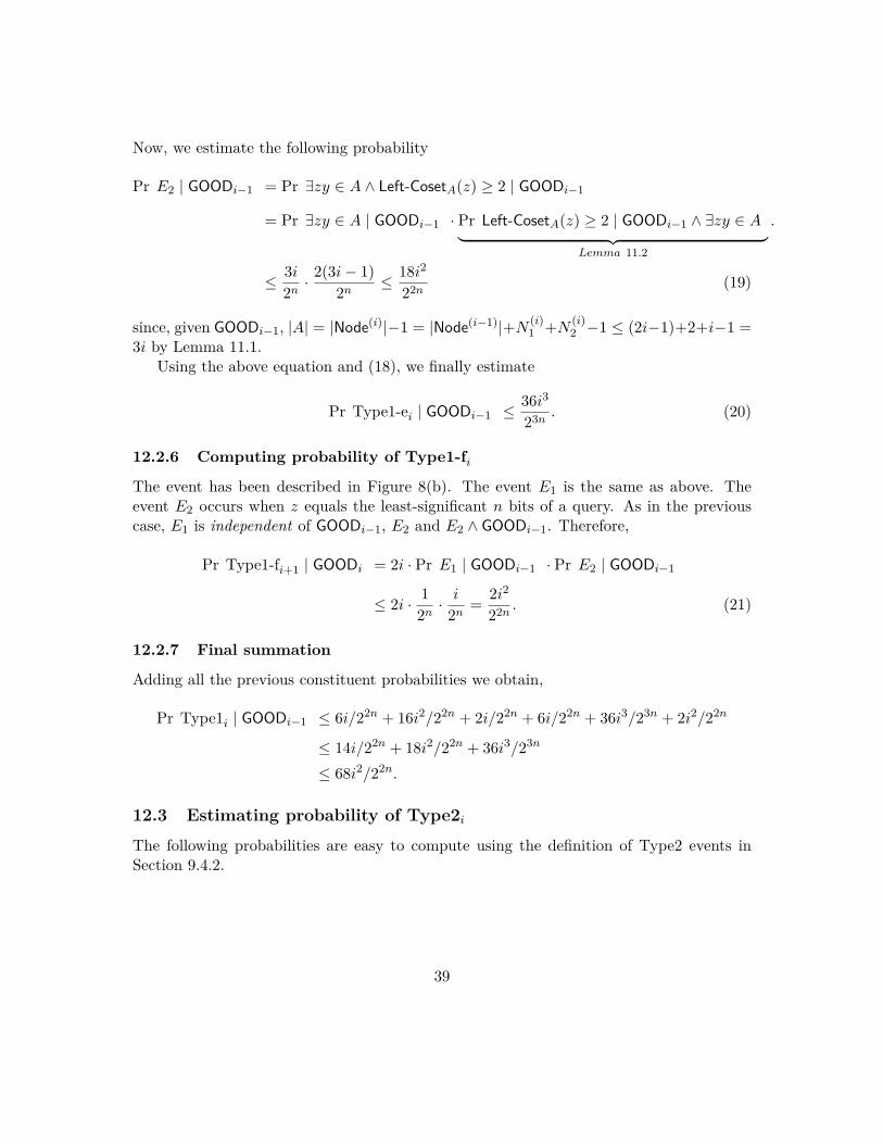
Now, we estimate the following probability

Pr E2 | GOODi−1 = Pr ∃zy ∈ A ∧ Left-CosetA(z) ≥ 2 | GOODi−1

= Pr ∃zy ∈ A | GOODi−1 · Pr Left-CosetA(z) ≥ 2 | GOODi−1 ∧ ∃zy ∈ A . - ._ -Lemma 11.2

3i 2(3i − 1) 18i2

≤ · ≤ (19)2n 2n 22n

(i) (i)since, given GOODi−1, |A| = |Node(i)|−1 = |Node(i−1)|+N +N −1 ≤ (2i−1)+2+i−1 = 1 2 3i by Lemma 11.1.

Using the above equation and (18), we finally estimate

Pr Type1-ei | GOODi−1 ≤ 36i3

. (20)23n

12.2.6 Computing probability of Type1-fi

The event has been described in Figure 8(b). The event E1 is the same as above. The event E2 occurs when z equals the least-significant n bits of a query. As in the previous case, E1 is independent of GOODi−1, E2 and E2 ∧ GOODi−1. Therefore,

Pr Type1-fi+1 | GOODi = 2i · Pr E1 | GOODi−1

≤ 2i · 1 2n ·

i 2n =

2i2

22n .

· Pr E2 | GOODi−1

(21)

12.2.7 Final summation

Adding all the previous constituent probabilities we obtain,

Pr Type1i | GOODi−1 ≤ 6i/22n + 16i2/22n + 2i/22n + 6i/22n + 36i3/23n + 2i2/22n

≤ 14i/22n + 18i2/22n + 36i3/23n

≤ 68i2/22n .


The following probabilities are easy to compute using the definition of Type2 events in Section 9.4.2.

39

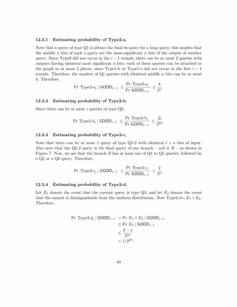
12.3.1 Estimating probability of Type2-ai

Note that a query of type Q1 is always the final ro-query for a long query; this implies that the middle n bits of such a query are the most-significant n bits of the output of another query. Since Type0 did not occur in the i − 1 rounds, there can be at most 2 queries with outputs having identical most significant n bits; each of these queries can be attached to the graph in at most 2 places, since Type1-b or Type1-e did not occur in the first i − 1 rounds. Therefore, the number of Q1 queries with identical middle n bits can be at most 4. Therefore,

Pr Type2-ai 8Pr Type2-ai | GOODi−1 ≤ ≤ .Pr GOODi−1 2n

12.3.2 Estimating probability of Type2-bi

Since there can be at most i queries of type Q2,

Pr Type2-bi 2iPr Type2-bi | GOODi−1 ≤ ≤ .Pr GOODi−1 22n

12.3.3 Estimating probability of Type2-ci

Note that there can be at most 1 query of type Q5-2 with identical . + n bits of input. Also note that the Q5-2 query is the final query of one branch – call it B – as shown in Figure 7. Now, we see that the branch B has at least one of Q1 to Q5 queries, followed by a Q5 or a Q6 query. Therefore,

Pr Type2-ci 2Pr Type2-ci | GOODi−1 ≤ ≤ .Pr GOODi−1 2n

12.3.4 Estimating probability of Type2-di

Let E1 denote the event that the current query is type Q3, and let E2 denote the event that the output is distinguishable from the uniform distribution. Now Type2-d= E1 ∧ E2. Therefore,

Pr Type2-di | GOODi−1 = Pr E1 ∧ E2 | GOODi−1

≤ Pr E2 | GOODi−1

2 − 1 ≤ 22n

= 1/22n .

40

12.3.5 Estimating probability of Type2-ei

Let E1 denote the event that the current query is type Q4, and let E2 denote the event that the output is distinguishable from the uniform distribution. Now Type2-e= E1 ∧ E2. Therefore,

Pr Type2-ei | GOODi−1 = Pr E1 ∧ E2 | GOODi−1


2 − 1 ≤ 22n

= 1/22n .

12.3.6 Estimating probability of Type2-fi

Let E1 denote the event that the current query is type Q5-1, and let E2 denote the event that the least significant n bits of output are distinguishable from the uniform distribution. Now Type2-f= E1 ∧ E2. Therefore,

Pr Type2-fi | GOODi−1 = Pr E1 ∧ E2 | GOODi−1


2 − 1 ≤ 2n

= 1/2n .



Pr Type2i | GOODi−1 ≤ 11/2n + 2/22n + 2i/22n ≤ 15/2n

≤ 30/2n .


Examining the definition of Type3 events in the following results can be established.

12.4.1 Estimating probability of Type3-ai

This event cannot occur – as observed in Section 9.4.3 – if Type1 event did not occur in the first i − 1 rounds. Therefore,

Pr Type3-ai | GOODi−1 = 0.

41

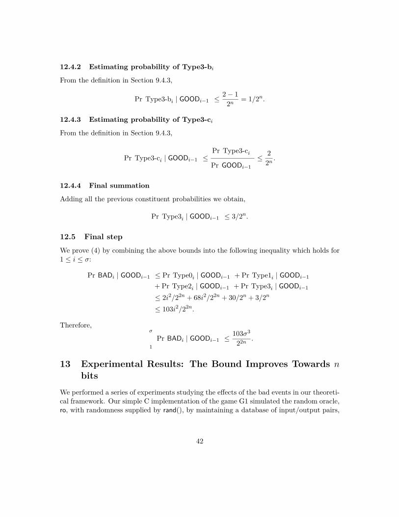
12.4.2 Estimating probability of Type3-bi

From the definition in Section 9.4.3,

2 − 1Pr Type3-bi | GOODi−1 ≤ = 1/2n .2n

12.4.3 Estimating probability of Type3-ci

From the definition in Section 9.4.3,

Pr Type3-ci 2Pr Type3-ci | GOODi−1 ≤ ≤ .2nPr GOODi−1



Pr Type3i | GOODi−1 ≤ 3/2n .

12.5 Final step

We prove (4) by combining the above bounds into the following inequality which holds for 1 ≤ i ≤ σ:

Pr BADi | GOODi−1 ≤ Pr Type0i | GOODi−1 + Pr Type1i | GOODi−1

+ Pr Type2i | GOODi−1 + Pr Type3i | GOODi−1

≤ 2i2/22n + 68i2/22n + 30/2n + 3/2n

≤ 103i2/22n .

Therefore, σ 103σ3

Pr BADi | GOODi−1 ≤ .22n 1

13 Experimental Results: The Bound Improves Towards n bits

We performed a series of experiments studying the effects of the bad events in our theoretical framework. Our simple C implementation of the game G1 simulated the random oracle, ro, with randomness supplied by rand(), by maintaining a database of input/output pairs,

42

assuring that ro commits to an output while allowing fresh queries to remain independent of all past events.

We collected data providing accurate estimates for the values Pr Type1i | GOODi−1

described in Section 9. Compiling these data we computed the relative percentage of several Type1 events. The results are provided in Table 13. The experimental results strongly agree with the bounds computed in Section 12.

In addition to these event probabilities, we calculated security bounds for several values of n. The computation was achieved by randomly generating a large number of graphs, Tro,

σand determining the number of queries, σ, required to cause i=1 Pr Type1i | GOODi−1 ≥ 0.5. The results of the experiments following this method are summarized in the blue line of Figure 9. Naturally, the data follow the theoretically obtained bound of σ = Ω(22n/3) (see Theorem 3.1). Some of the values in the graph are slightly lower than 2/3, due to the effect of constants. The data asymptotically approach 2/3.

We did not consider the Type2 and Type3 events, since, for any efficient adversary the probabilities of these events are dominated by that of the Type1 events. We found that choosing the values at which to place the 1st query uniformly at random from among all possible maximal left-cosets was the most advantageous strategy for an adversary.

Hoping that the real indifferentiability security bound is more than 2n/3-bit, we experimented with a smaller set of ‘bad’ events than the ones described in Section 9. We first removed the ‘artificial’ Type1-b, Type1-e, and Type0 events; it is easy to see that (2) and (3) can be proved without these events. These events were inserted so that it is mathematically easier to derive the bounds on the size of the graph Tro (see Section 11). It is our intuition that a cleverer mathematician will be able to obtain similar bounds even without these ‘artificial’ events. Then we have switched from the two-phase framework to a natural extension of three-phase (or multi-phase) framework. In short, with the construction of a multi-phase version of the game G1, removing the artificial Type1-b, Type1-e, and Type0 events, we see that the normalized logarithm of σ increases towards one as n increases. The Type1 events of the three-phase version of G1 are illustrated in Figure 10. These data indicate that the bound may be significantly improved, possibly even to nearly n bits, as reflected in the red line of Figure 9.

14 Conclusion and Open Problems

Indifferentiability security guarantees absence of all generic attacks. In this paper we improved the indifferentiability security bound of the FWP hash mode from n/2 to 2n/3 bits. Many popular hash modes use primitives of the form C : {0, 1}2n → {0, 1}2n. For such an important family, the FWP becomes the only mode to achieve indifferentiable security of more than n/2 bits. Secondly, among n-bit hash modes with a > 2n, the FWP mode has the highest rate among all modes which have beyond-birthday-barrier security. Our experimental results strongly indicate that the bound could be further improved, possibly

43

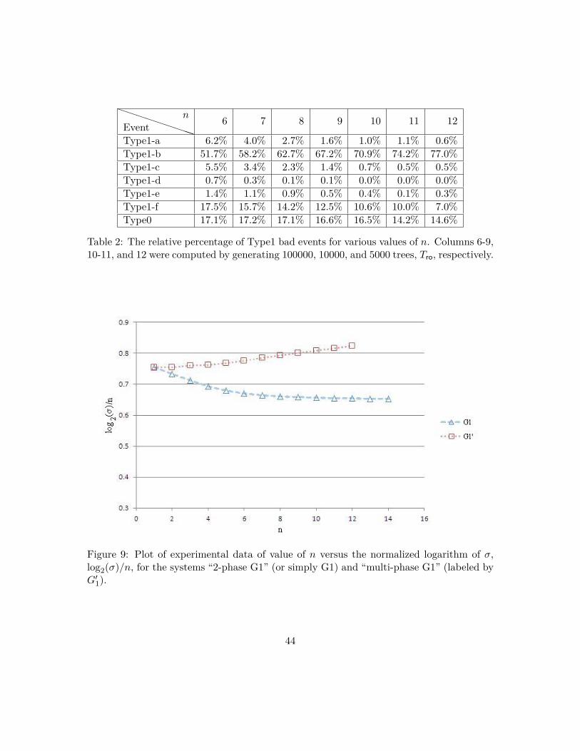
��Event n 6 7 8 9 10 11 12

Type1-a 6.2% 4.0% 2.7% 1.6% 1.0% 1.1% 0.6% Type1-b 51.7% 58.2% 62.7% 67.2% 70.9% 74.2% 77.0% Type1-c 5.5% 3.4% 2.3% 1.4% 0.7% 0.5% 0.5% Type1-d 0.7% 0.3% 0.1% 0.1% 0.0% 0.0% 0.0% Type1-e 1.4% 1.1% 0.9% 0.5% 0.4% 0.1% 0.3% Type1-f 17.5% 15.7% 14.2% 12.5% 10.6% 10.0% 7.0% Type0 17.1% 17.2% 17.1% 16.6% 16.5% 14.2% 14.6%

Table 2: The relative percentage of Type1 bad events for various values of n. Columns 6-9, 10-11, and 12 were computed by generating 100000, 10000, and 5000 trees, Tro, respectively.

Figure 9: Plot of experimental data of value of n versus the normalized logarithm of σ, log2(σ)/n, for the systems “2-phase G1” (or simply G1) and “multi-phase G1” (labeled by G ' 1).

44

Type1-a

Node-collision

1stph

ase New

ycy′c

m

y y′

y∗

Old

==

Type1-b

Query collision(2n bits)

New

yc y′c m

y y′

y∗

==

Old

2ndph

ase

New

yc y′c m

y

y∗

Type1-c

y′

Old1 Old2

m′

z z′==

=

Node collisionQuery collision

(2n bits)

Type1-d

New

yc y′c m

y

y∗

y′

Old1

m′

z z′

==

=

Old2

random n bits

n bits

l − n bits

l bits

= n bit equality

== 2n bit equality

Notation3rdph

ase

New

yc y′c m

y

y∗

Type1-e

y′

Old1

m′

z z′==

=

Old2

=

Old3

New

yc y′c m

y

y∗

y′

Old1

m′

z z′

=

Old2

=

Type1-f

Node collision

Old3

=

Query collision (n bits)

Figure 10: The Type1 events of the 3-phase version of the system G1.

45

even close to n bits. In addition, our proof technique is novel, and it uses only three games with a set of specially designed bad events.

Our work leaves room for more research. The security upper-bound for the FWP is n-bit, while the proven lower-bound is 2

3 n-bit. One research direction would be to close the gap between these upper and lower bounds. Also, one may try to optimize the complexity of the simulator running time.

Acknowledgment

We would like to thank Donghoon Chang, Mridul Nandi, Tom Shrimpton, Cristina Tone, Meltem Sönmez Turan, and the Keccak team for their suggestions and remarks which helped a lot to improve the quality of the paper.

References

[1] Elena Andreeva, Charles Bouillaguet, Pierre-Alain Fouque, Jonathan J. Hoch, John Kelsey, Adi Shamir, and Sébastien Zimmer. Second preimage attacks on dithered hash functions. In Smart [35], pages 270–288. (Cited on page 5.)

[2] Elena Andreeva, Atul Luykx, and Bart Mennink. Provable Security of BLAKE with Non-Ideal Compression Function. Cryptology ePrint Archive, Report 2011/620, 2011. http://eprint.iacr.org/. (Cited on page 6.)

[3] Elena Andreeva, Atul Luykx, and Bart Mennink. Provable Security of BLAKE with Non-Ideal Compression Function. 3rd SHA-3 Candidate Conference, 2012. (Cited on page 5.)

[4] Elena Andreeva, Bart Mennink, and Bart Preneel. On the Indifferentiability of the Grøstl Hash Function. In Juan A. Garay and Roberto De Prisco, editors, SCN, volume 6280 of Lecture Notes in Computer Science, pages 88–105. Springer, 2010. (Cited on page 7.)

[5] Elena Andreeva, Bart Mennink, and Bart Preneel. The Parazoa Family: Generalizing the Sponge Hash Functions. IACR Cryptology ePrint Archive, 2011:28, 2011. (Cited on page 6.)

[6] Mihir Bellare and Thomas Ristenpart. Multi-Property-Preserving Hash Domain Extension and the EMD Transform. In Xuejia Lai and Kefei Chen, editors, ASIACRYPT 2006, volume 4284 of Lecture Notes in Computer Science, pages 299–314. Springer, 2006. (Cited on page 6.)

[7] Guido Bertoni, Joan Daemen, Michaël Peeters, and Gilles Van Assche. Sponge Functions. ECRYPT 2007, 2007. http://sponge.noekeon.org/SpongeFunctions.pdf. Accessed March 2012. (Cited on page 7.)

46

http://eprint.iacr.org/

http://sponge.noekeon.org/SpongeFunctions.pdf

[8] Guido Bertoni, Joan Daemen, Michaël Peeters, and Gilles Van Assche. On the Indifferentiability of the Sponge Construction. In Smart [35], pages 181–197. (Cited on page 6.)

[9] Rishiraj Bhattacharyya, Avradip Mandal, and Mridul Nandi. Security Analysis of the Mode of JH Hash Function. In Seokhie Hong and Tetsu Iwata, editors, FSE, volume 6147 of Lecture Notes in Computer Science, pages 168–191. Springer, 2010. (Cited on pages 5, 6 and 7.)

[10] Eli Biham and Orr Dunkelman. A framework for iterative hash functions – HAIFA. Second NIST Cryptographic Hash Workshop, 2006, 2006. (Cited on page 6.)

[11] Simon R. Blackburn, Douglas R. Stinson, and Jalaj Upadhyay. On the complexity of the herding attack and some related attacks on hash functions. Des. Codes Cryptography, 64(1-2):171–193, 2012. (Cited on page 5.)

[12] Gilles Brassard, editor. Advances in Cryptology - CRYPTO ’89, 9th Annual International Cryptology Conference, Santa Barbara, California, USA, August 20-24, 1989, Proceedings, volume 435 of Lecture Notes in Computer Science. Springer, 1990. (Cited on pages 47 and 49.)

[13] E. Bresson, A. Canteaut, B. Chevallier-Mames, C .Clavier, T. Fuhr, A. Gouget, T. Icart, J.-F. Misarsky, M. Naya-Plasencia, P. Paillier, T. Pornin, J.-R. Reinhard, C. Thuillet, and M. Videau. SHABAL. The 1st SHA-3 Candidate Conference. (Cited on page 6.)

[14] Donghoon Chang and Mridul Nandi. Improved indifferentiability security analysis of chopMD hash function. In Kaisa Nyberg, editor, FSE, volume 5086 of Lecture Notes in Computer Science, pages 429–443. Springer, 2008. (Cited on page 6.)

[15] Donghoon Chang, Mridul Nandi, and Moti Yung. Indifferentiability of the Hash Algorithm BLAKE. Cryptology ePrint Archive, Report 2011/623, 2011. http:// eprint.iacr.org/. (Cited on pages 5 and 6.)

[16] Jean-Sébastien Coron. Optimal security proofs for pss and other signature schemes. In Lars R. Knudsen, editor, EUROCRYPT, volume 2332 of Lecture Notes in Computer Science, pages 272–287. Springer, 2002. (Cited on page 5.)

[17] Jean-Sébastien Coron, Yevgeniy Dodis, Cécile Malinaud, and Prashant Puniya. Merkle-Damgård Revisited: How to Construct a Hash Function. In Victor Shoup, editor, CRYPTO 2005, volume 3621 of Lecture Notes in Computer Science, pages 430–448. Springer, 2005. (Cited on pages 5, 6 and 10.)

[18] Ivan Damgård. A Design Principle for Hash Functions. In Brassard [12], pages 416– 427. (Cited on page 6.)

47



[19] Ewan Fleischmann, Michael Gorski, and Stefan Lucks. Some Observations on Indifferentiability. In Ron Steinfeld and Philip Hawkes, editors, ACISP, volume 6168 of Lecture Notes in Computer Science, pages 117–134. Springer, 2010. (Cited on pages 5 and 11.)

[20] P. Gauravaram, L. Knudsen, K. Matusiewicz, F. Mendel, C. Rechberger, M. Schlaffer, and S. Thomsen. Groestl - a SHA-3 candidate. The 1st SHA-3 Candidate Conference. (Cited on page 6.)

[21] Shoichi Hirose, Je Hong Park, and Aaram Yun. A Simple Variant of the Merkle-Damgård Scheme with a Permutation. In Kaoru Kurosawa, editor, ASIACRYPT, volume 4833 of Lecture Notes in Computer Science, pages 113–129. Springer, 2007. (Cited on page 6.)

[22] Jonathan J. Hoch and Adi Shamir. Breaking the ICE - Finding Multicollisions in Iterated Concatenated and Expanded (ICE) Hash Functions. In Matthew J. B. Robshaw, editor, FSE, volume 4047 of Lecture Notes in Computer Science, pages 179–194. Springer, 2006. (Cited on page 5.)

[23] Antoine Joux. Multicollisions in Iterated Hash Functions: Application to Cascaded Constructions. In Matthew K. Franklin, editor, CRYPTO 2004, volume 3152 of Lecture Notes in Computer Science, pages 306–316. Springer, 2004. (Cited on pages 5 and 6.)

[24] John Kelsey and Tadayoshi Kohno. Herding Hash Functions and the Nostradamus Attack. In Serge Vaudenay, editor, EUROCRYPT, volume 4004 of Lecture Notes in Computer Science, pages 183–200. Springer, 2006. (Cited on page 5.)

[25] John Kelsey and Bruce Schneier. Second Preimages on n-Bit Hash Functions for Much Less than 2n Work. In Ronald Cramer, editor, EUROCRYPT 2005, volume 3494 of Lecture Notes in Computer Science, pages 474–490. Springer, 2005. (Cited on page 5.)

[26] Stefan Lucks. A failure-friendly design principle for hash functions. In Bimal K. Roy, editor, ASIACRYPT, volume 3788 of Lecture Notes in Computer Science, pages 474–494. Springer, 2005. (Cited on pages 6 and 7.)

[27] Ueli M. Maurer, Renato Renner, and Clemens Holenstein. Indifferentiability, impossibility results on reductions, and applications to the random oracle methodology. In Moni Naor, editor, TCC, volume 2951 of Lecture Notes in Computer Science, pages 21–39. Springer, 2004. (Cited on page 5.)

[28] Ueli M. Maurer, Renato Renner, and Clemens Holenstein. Indifferentiability, impossibility results on reductions, and applications to the random oracle methodology. In TCC, pages 21–39, 2004. (Cited on page 11.)

48

[29] Ralph C. Merkle. One Way Hash Functions and DES. In Brassard [12], pages 428–446. (Cited on page 6.)

[30] Dustin Moody, Souradyuti Paul, and Daniel Smith-Tone. Improved Indifferentiability Security Bound for the JH Mode. 3rd SHA-3 Candidate Conference, 2012. (Cited on pages 6 and 7.)

[31] Mridul Nandi and Souradyuti Paul. Speeding up the wide-pipe: Secure and fast hashing. In Guang Gong and Kishan Chand Gupta, editors, INDOCRYPT, volume 6498 of Lecture Notes in Computer Science, pages 144–162. Springer, 2010. (Cited on pages 6, 7 and 10.)

[32] Mridul Nandi and Douglas R. Stinson. Multicollision Attacks on Some Generalized Sequential Hash Functions. IEEE Transactions on Information Theory, 53(2):759– 767, 2007. (Cited on page 5.)

[33] Thomas Ristenpart, Hovav Shacham, and Thomas Shrimpton. Careful with Composition: Limitations of the Indifferentiability Framework. In Kenneth G. Paterson, editor, EUROCRYPT, volume 6632 of Lecture Notes in Computer Science, pages 487–506. Springer, 2011. (Cited on pages 5 and 11.)

[34] Victor Shoup. OAEP Reconsidered. In Joe Kilian, editor, CRYPTO, volume 2139 of Lecture Notes in Computer Science, pages 239–259. Springer, 2001. (Cited on page 5.)

[35] Nigel P. Smart, editor. Advances in Cryptology - EUROCRYPT 2008, 27th Annual International Conference on the Theory and Applications of Cryptographic Techniques, Istanbul, Turkey, April 13-17, 2008. Proceedings, volume 4965 of Lecture Notes in Computer Science. Springer, 2008. (Cited on pages 46 and 47.)

[36] Hongjun Wu. The JH Hash Function. The 1st SHA-3 Candidate Conference (2009). (Cited on page 6.)

A Definitions

Definition A.1 (Random oracle) A random oracle is a function RO : X → Y chosen uniformly at random from the set of all |Y ||X| functions that map X → Y . In other words, a function RO : X → Y is a random oracle if and only if, for each x ∈ X, the value of RO(x) is chosen uniformly at random from Y .

49

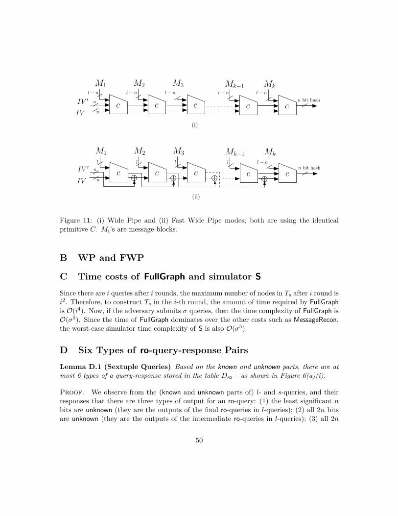
c

M1l − n

n

nIV ′

IVc

M2

c

M3l − n l − n

c

Mk−1

c

Mkl − n

n bit hash

(i)

c

M1

l

n

nIV ′

IVc

M2

c

M3

l l

c

Mk−1

c

Mk

l − nn bit hash

(ii)

l

l − n

Figure 11: (i) Wide Pipe and (ii) Fast Wide Pipe modes; both are using the identical primitive C. Mi’s are message-blocks.

B WP and FWP

C Time costs of FullGraph and simulator S

Since there are i queries after i rounds, the maximum number of nodes in Ts after i round is i2. Therefore, to construct Ts in the i-th round, the amount of time required by FullGraph is O(i4). Now, if the adversary submits σ queries, then the time complexity of FullGraph is O(σ5). Since the time of FullGraph dominates over the other costs such as MessageRecon, the worst-case simulator time complexity of S is also O(σ5).

D Six Types of ro-query-response Pairs

Lemma D.1 (Sextuple Queries) Based on the known and unknown parts, there are at most 6 types of a query-response stored in the table Dro – as shown in Figure 6(a)(i).

Proof. We observe from the (known and unknown parts of) l- and s-queries, and their responses that there are three types of output for an ro-query: (1) the least significant n bits are unknown (they are the outputs of the final ro-queries in l-queries); (2) all 2n bits are unknown (they are the outputs of the intermediate ro-queries in l-queries); (3) all 2n

50

bits are known (they are the outputs of the s-queries. Note that in case (1), the output can be of three types of input (Q1, Q2 and Q5); any extra type of input for this output will require at least four types of output in total, which is impossible. Case (2) output can have two types of input (Q3 and Q4). Finally, for case (3), an output can have only one type of input (Q6). Altogether, there are six types of query-response pairs. �

E Proof of (8) Let V 1 and V 2 denote the views of the systems G1, and G2 respectively, after i queriesi i have been processed. To prove (8), it suffices to show that given GOOD1σ, the views V 1

σ and V 2 are identically distributed. We do this by induction on the number of queries σ.σ

Induction Hypothesis: Given GOOD1i, V 1 and V 2 are identically distributed. i i

Base: When i = 0, then no query has been made; therefore the hypothesis is true.

Induction Step: Now assume the induction hypothesis holds. We have to show that if GOOD1i+1 occurred, then Vi

1+1 and Vi

2+1 are identically distributed.

Let (Ii1+1, Oi

1+1) and (Ii

2+1, Oi

2+1) denote the input-output pairs for the systems G1 and G2

respectively in the i + 1st round. A little reflection shows that proving the induction step is equivalent to proving the

following proposition.

Proposition E.1 (Proof of Induction Step) Given GOOD1i+1 and V 1 = V 2 i i

1. the input-views Ii1+1 and Ii

2+1 are identically distributed;

2. if I1 = Ii2+1 then the output-views Oi

1+1 and Oi

2+1 are identically distributed. i+1

Proof. 1. This result is easy since V 1 = V 2.i i

2. First, we establish the following lemma which is the main ingredient in our proof.

Lemma E.2 The reconstruction graphs Ts of the systems G1 and G2 are isomorphic after i rounds, given GOODi and V 1 = V 2.i i

Proof. For each fresh ro-query, the graph Tro of system G1 is augmented in two phases (see Figure 5). In these two phases, all possible nodes are added to the graph Tro. An analysis of the Type1-a,c,d and f events show that if these events do not occur then no

51

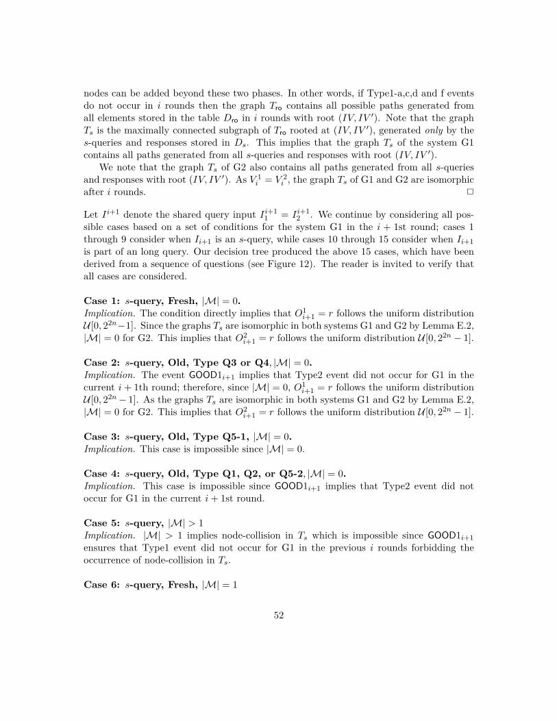
nodes can be added beyond these two phases. In other words, if Type1-a,c,d and f events do not occur in i rounds then the graph Tro contains all possible paths generated from all elements stored in the table Dro in i rounds with root (IV, IV '). Note that the graph Ts is the maximally connected subgraph of Tro rooted at (IV, IV '), generated only by the s-queries and responses stored in Ds. This implies that the graph Ts of the system G1 contains all paths generated from all s-queries and responses with root (IV, IV ').

We note that the graph Ts of G2 also contains all paths generated from all s-queries and responses with root (IV, IV '). As V 1 = V 2, the graph Ts of G1 and G2 are isomorphic i i after i rounds. �

= Ii+1Let Ii+1 denote the shared query input Ii+1 . We continue by considering all pos1 2 sible cases based on a set of conditions for the system G1 in the i + 1st round; cases 1 through 9 consider when Ii+1 is an s-query, while cases 10 through 15 consider when Ii+1

is part of an long query. Our decision tree produced the above 15 cases, which have been derived from a sequence of questions (see Figure 12). The reader is invited to verify that all cases are considered.

Case 1: s-query, Fresh, |M| = 0. Implication. The condition directly implies that O1 = r follows the uniform distribution i+1 U [0, 22n −1]. Since the graphs Ts are isomorphic in both systems G1 and G2 by Lemma E.2, |M| = 0 for G2. This implies that O2 = r follows the uniform distribution U [0, 22n − 1].i+1

Case 2: s-query, Old, Type Q3 or Q4, |M| = 0. Implication. The event GOOD1i+1 implies that Type2 event did not occur for G1 in the current i + 1th round; therefore, since |M| = 0, O1 = r follows the uniform distribution i+1 U [0, 22n − 1]. As the graphs Ts are isomorphic in both systems G1 and G2 by Lemma E.2, |M| = 0 for G2. This implies that O2 = r follows the uniform distribution U [0, 22n − 1].i+1

Case 3: s-query, Old, Type Q5-1, |M| = 0. Implication. This case is impossible since |M| = 0.

Case 4: s-query, Old, Type Q1, Q2, or Q5-2, |M| = 0. Implication. This case is impossible since GOOD1i+1 implies that Type2 event did not occur for G1 in the current i + 1st round.

Case 5: s-query, |M| > 1 Implication. |M| > 1 implies node-collision in Ts which is impossible since GOOD1i+1

ensures that Type1 event did not occur for G1 in the previous i rounds forbidding the occurrence of node-collision in Ts.

Case 6: s-query, Fresh, |M| = 1

52

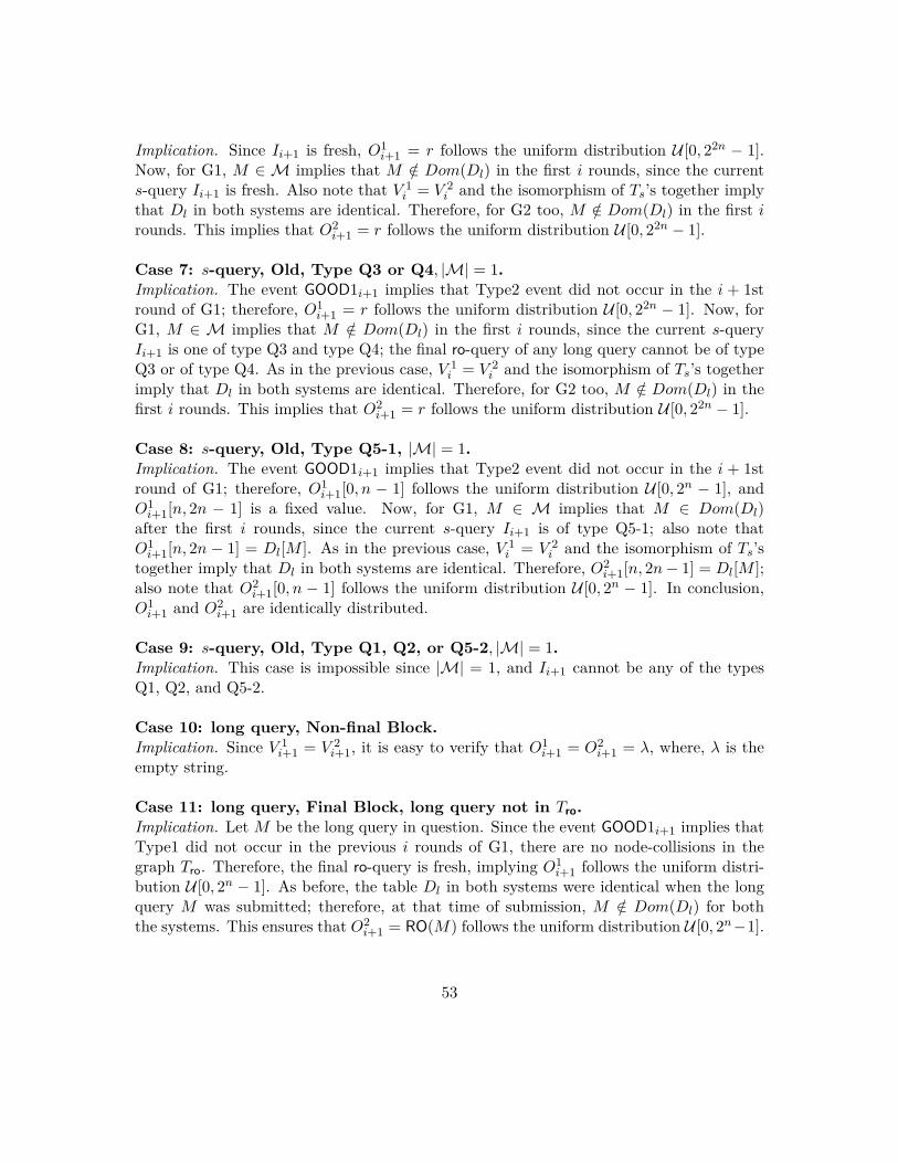
Implication. Since Ii+1 is fresh, O1 = r follows the uniform distribution U [0, 22n − 1].i+1 Now, for G1, M ∈ M implies that M /∈ Dom(Dl) in the first i rounds, since the current s-query Ii+1 is fresh. Also note that V 1 = V 2 and the isomorphism of Ts’s together imply i i that Dl in both systems are identical. Therefore, for G2 too, M /∈ Dom(Dl) in the first i rounds. This implies that O2 = r follows the uniform distribution U [0, 22n − 1].i+1

Case 7: s-query, Old, Type Q3 or Q4, |M| = 1. Implication. The event GOOD1i+1 implies that Type2 event did not occur in the i + 1st round of G1; therefore, Oi

1+1 = r follows the uniform distribution U [0, 22n − 1]. Now, for

G1, M ∈ M implies that M ∈/ Dom(Dl) in the first i rounds, since the current s-query Ii+1 is one of type Q3 and type Q4; the final ro-query of any long query cannot be of type Q3 or of type Q4. As in the previous case, V 1 = V 2 and the isomorphism of Ts’s together i i imply that Dl in both systems are identical. Therefore, for G2 too, M /∈ Dom(Dl) in the first i rounds. This implies that O2 = r follows the uniform distribution U [0, 22n − 1].i+1

Case 8: s-query, Old, Type Q5-1, |M| = 1. Implication. The event GOOD1i+1 implies that Type2 event did not occur in the i + 1st round of G1; therefore, Oi

1+1[0, n − 1] follows the uniform distribution U [0, 2n − 1], and

Oi1+1[n, 2n − 1] is a fixed value. Now, for G1, M ∈ M implies that M ∈ Dom(Dl)

after the first i rounds, since the current s-query Ii+1 is of type Q5-1; also note that Oi

1+1[n, 2n − 1] = Dl[M ]. As in the previous case, V 1 = V 2 and the isomorphism of Ts’si i

together imply that Dl in both systems are identical. Therefore, Oi2+1[n, 2n − 1] = Dl[M ];

also note that Oi2+1[0, n − 1] follows the uniform distribution U [0, 2n − 1]. In conclusion,

Oi1+1 and Oi

2+1 are identically distributed.

Case 9: s-query, Old, Type Q1, Q2, or Q5-2, |M| = 1. Implication. This case is impossible since |M| = 1, and Ii+1 cannot be any of the types Q1, Q2, and Q5-2.

Case 10: long query, Non-final Block. Implication. Since V 1 = Vi

2+1, it is easy to verify that O1 = O2 = λ, where, λ is the i+1 i+1 i+1

empty string.

Case 11: long query, Final Block, long query not in Tro. Implication. Let M be the long query in question. Since the event GOOD1i+1 implies that Type1 did not occur in the previous i rounds of G1, there are no node-collisions in the graph Tro. Therefore, the final ro-query is fresh, implying Oi

1+1 follows the uniform distri

bution U [0, 2n − 1]. As before, the table Dl in both systems were identical when the long query M was submitted; therefore, at that time of submission, M ∈/ Dom(Dl) for both the systems. This ensures that O2 = RO(M) follows the uniform distribution U [0, 2n −1].i+1

53

Case 12: long query, Final Block, long query in Tro, long query in Ts. Implication. Since the graph Ts in both systems are isomorphic by Lemma E.2, O1 = i+1 Oi

2+1.

Case 13, 14 and 15: long query, Final Block, long query in Tro, long query not in Ts. Ii+1 is the final message-block of a long query (denoted by M) which forms a red branch (see Section 9.4 and Figure 6(b)).

Case 13: Final ro-query is Type Q1, Q2 or Q5. Implication. Note that this case implies a node collision in Tro. By definition, the ro-query

' yk−1yk−1mk is already the final ro-query of a previous long query since it is of type Q1, Q2 'and Q5; now, yk−1yk−1mk is also the final ro-query of the current long query M . Hence

the collision in Tro. This case is impossible since GOOD1i+1 implies that Type1 event did not occur in the first i rounds; therefore Tro cannot have a node-collision.

Case 14: Final ro-query is Type Q3 or Q5. Implication. Since the event Type3 did not occur in the i + 1st round, Oi

1+1 follows the

uniform distribution U [0, 2n − 1]. Now, for G1, the long query M ∈/ Dom(Dl) when M was submitted since the final ro-query of any long query cannot be of type Q3 or Q4. As the table Dl of both systems are identical, for G2, M /∈ Dom(Dl) when M was submitted. Therefore, O2 = RO(M) follows the uniform distribution U [0, 2n − 1].i+1

Case 15: Final ro-query is Type Q6, and an intermediate query is Type Q1, Q2, Q3, Q4 or Q5. Implication. This case is impossible since Type3 in the i + 1st round did not occur.

To conclude, in all 15 cases above we have shown that the outputs Oi1+1 and O2 arei+1

identically distributed if the variable BAD is not set. This completes the proof. �

54

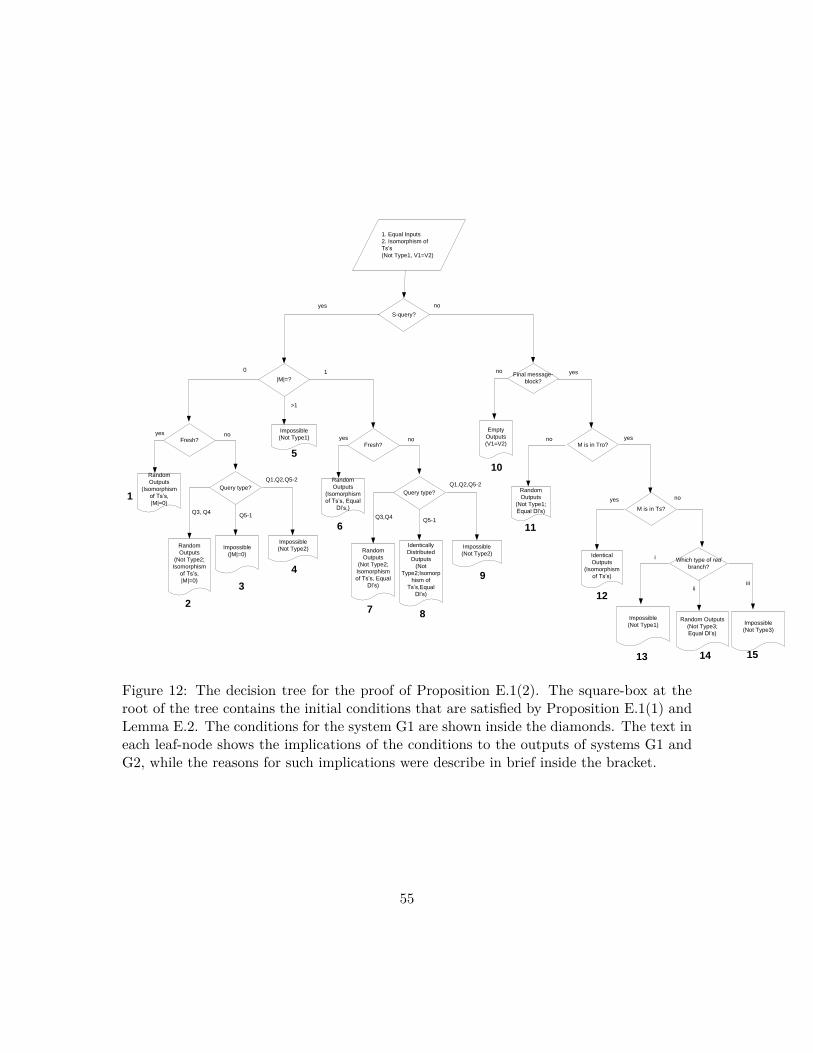
S-query?

|M|=?

0 1

Impossible

(Not Type1)

>1

yes no

Final message-

block?

Empty

Outputs

(V1=V2)

no yes

M is in Tro?

yesno

M is in Ts?

Random

Outputs

(Not Type1;

Equal Dl’s)

yes no

Identical

Outputs

(Isomorphism

of Ts’s)

Random

Outputs

(Isomorphism

of Ts’s, Equal

Dl’s,)

1. Equal Inputs

2. Isomorphism of

Ts’s

(Not Type1, V1=V2)

Fresh?

Identically

Distributed

Outputs

(Not

Type2;Isomorp

hism of

Ts’s,Equal

Dl’s)

yes no

Query type?

Random

Outputs

(Not Type2;

Isomorphism

of Ts’s, Equal

Dl’s)

Q5-1Q3,Q4

Q1,Q2,Q5-2

Impossible

(Not Type2)

Random

Outputs

(Isomorphism

of Ts’s,

|M|=0)

Fresh?

Impossible

(|M|=0)

yes no

Query type?

Random

Outputs

(Not Type2;

Isomorphism

of Ts’s,

|M|=0)

Q5-1Q3, Q4

Q1,Q2,Q5-2

Impossible

(Not Type2)

Which type of red

branch?

i

iiiii

Impossible

(Not Type1)Random Outputs

(Not Type3;

Equal Dl’s)

Impossible

(Not Type3)

1

2

3

4

5

6

7 8

9

10

11

12

13 14 15

Figure 12: The decision tree for the proof of Proposition E.1(2). The square-box at the root of the tree contains the initial conditions that are satisfied by Proposition E.1(1) and Lemma E.2. The conditions for the system G1 are shown inside the diamonds. The text in each leaf-node shows the implications of the conditions to the outputs of systems G1 and G2, while the reasons for such implications were describe in brief inside the bracket.

55

indifferentiability security of the fast widepipe hash

Documents