indicators, tools and method for metropolitan footprint tools · d3.3 indicators, tools and method...

D3.3 Indicators, Tools and Method for the Metropolitan Footprint Tools

1

D3.3

Indicators, Tools and Method for Metropolitan Footprint Tools

Main Authors: Dirk Wascher, Ingo Zasada, Leonne Jeurissen, Gustavo Arciniegas, Jaap de Kroes, Guido Sali, Stefano Corsi, Federica Monaco, Ulrich Schmutz, Matjaz Glavan, Dirk Pohle and Michiel van Eupen

Reviewer:

Due date of deliverable: 15 September 2014

Actual submission date: 30 July 2015

Keywords: Ecological footprint, metropolitan regions, food security, landscape planning, recreation, serious gaming, land use change


2

Contents

1 Introduction .............................................................................................................................. 3

1.1 Global Hectares vs. Local Hectares................................................................................... 3

2 Footprint basics: demand and supply ....................................................................................... 7

2.1 Analysis of demand .......................................................................................................... 7

2.2 Analysis of supply ............................................................................................................. 9

2.3 Building upon existing footprint tools ............................................................................ 10

2.3.1 The European Ecological Footprint Tool ................................................................ 10

2.3.2 The Urban Footprint Tool....................................................................................... 12

2.4 Conclusions ..................................................................................................................... 14

3 Metropolitan footprint tools................................................................................................... 14

3.1 Introduction .................................................................................................................... 14

3.2 Metropolitan Area Profile and Scenario (MAPS) tool .................................................... 16

3.2.1 Modelling Procedure and Database ....................................................................... 17

3.2.2 Spatial modeling ..................................................................................................... 20

3.2.3 MAPS Application ................................................................................................... 20

3.2.4 Metropolitan Self-sufficiency ................................................................................. 23

3.2.5 Scenario Application .............................................................................................. 25

3.3 Metropolitan Foodscape Planner (MFP) supply tool ..................................................... 27

3.3.1 Data and indicators ................................................................................................ 27

3.3.2 The MFP spatial zoning framework........................................................................ 29

3.3.3 GIS operations and calculations to arrive at the MFP zones ................................. 32

3.3.4 Land cover disaggregation towards HSMU commodity groups ............................. 34

3.3.5 MFP-tool configuration of the digital MAPTABLE .................................................. 35

3.4 Tool output ..................................................................................................................... 38

3.4.1 Rotterdam City-Region ........................................................................................... 38

3.4.2 London Metropolitan Region ................................................................................. 41

3.4.3 Berlin-Brandenburg ................................................................................................ 42

3.4.4 Milano .................................................................................................................... 44

3.4.5 Ljubljana ................................................................................................................. 45

4 Discussion ............................................................................................................................... 46

4.1 Summary ........................................................................................................................ 46

4.2 Towards a new food system paradigm .......................................................................... 48

4.3 Further Research ............................................................................................................ 50

4.4 Conclusion ...................................................................................................................... 51

5 References .............................................................................................................................. 53

ANNEX 1: validation figures from comparing HSMU data with LGN7 crop data ............................ 56


3

1 Introduction 1.1 Global Hectares vs. Local Hectares The European Sustainable Development Strategy (CEC 2001, CEU 2006) addresses a broad range of ‘unsustainable trends’ ranging from public health, poverty and social exclusion to climate change, energy use and management of natural resources. A key objective of the SDS is to promote development that does not exceed ecosystem carrying capacity and to decouple economic growth from negative environmental impacts. A report commissioned by the European Commission (2008) came to the conclusion that the Ecological Footprint should be used by EU institutions within the Sustainable Development Indicators (SDI) framework.

Figure 1: Ecological footprint (EF) in global and local hectares for London, Rotterdam City Region, Berlin, Milano, Ljubljana and Nairobi1. Large dark circles as global hectares and small blue circles as local hectares showing the land requirements in terms of food production areas based on national accounts.

The Ecological Footprint measures how much biologically productive land and water area is required to provide the resources consumed and absorb the wastes generated by a human population, taking into account prevailing technology. The

1 Calculations of both global and local hectares for Milano, Ljubljana and Nairobi are based on estimates.


4

annual production of biologically provided resources, called bio-capacity, is also measured as part of the methodology. The Ecological Footprint and bio-capacity are each measured in global hectares, a standardized unit of measurement equal to 1 hectare with global average productivity (CEC 2008).

However, due to a fragmented research history with simultaneous and largely uncoordinated efforts across sectors, research institutes and regions, ecological footprint calculations are manifold and differ substantially in terms of underlying data and methodologies (see Table 3). While the ecological footprint is still considered as a key reference and communication tool when comparing environmental impacts at highly aggregated levels, the above mentioned inconsistencies have been a matter of concern for both research and policy. With the emergence of the European Footprint Tool (Briggs 2011) this situation has clearly improved. The new, internet-based assessment tool offers a harmonized methodology for all 27 EU countries plus another 16 countries and regions of the world which allows statistical modelling and even scenario developments for different sectors, among which food consumption impacts, as global hectares (see Table 1).

Table 1: Ecological footprints in global and local hectares based on the population figures for the six case study areas

Sources:

* EUREAPA online scenario modelling and policy assessment tool (Briggs et al. 2011) ** National references and estimates based on EFSA (2011) *** EUREAPA data for S-Africa & estimates

Another challenge of the ecological footprint approach is the abstract dimension of its currency – the global hectares which represent the total impact of certain economic sectors and activities as the sum of all processes along the production chain – in this case the food chain from farm to fork. This includes all energy, water, land and material input resources such as fertilizers, machinery and packing material that occur along the full food chain. Using global hectares as a normalized unit allows Ecological Footprints to be expressed in comparable area terms, despite differences in bio-productivity among land types, regions and countries. EUREAPA tracks the use of six categories of productive areas: cropland, grazing land, fishing grounds, forest area, built-up land, and carbon demand on land. The translation into global hectares


5

uses yield factors and equivalence factors, which relate the bio-productivity of each land type to the global average bio-productivity. Because the bio-productivity of land types varies by country, yield factors are used to relate national yields in each category of land to the global average yields. Equivalence factors adjust for the relative productivity of the six categories of land and water area. EUREAPA figures have been used to illustrate the global hectare requirements of the six case study areas in comparison to local hectares based on different references (see Table 1 and Figure 1). The annual production of biologically provided resources, called bio-capacity, is also measured as part of the Ecological Footprint methodology, and is also accounted for in terms of global hectares. While global hectares can be considered as a typical dimension of evidence-based impact assessments, the associated land demands appear rather virtual in terms of their spatial-geographic explicitness.

Here is where the FOODMETRES’ metropolitan footprint tools come in. Rather than relying on global hectares as the basis for communicating the impacts of urban food consumption, these tools are meant to translate the principles of the available ‘bio-capacity’ into a spatially explicit reference base that manages both ‘demand’ and ‘supply’ data simultaneously at the scale of metropolitan regions. For this purpose we have developed two distinct, yet complementary tools:

- the regional Metropolitan Area Profiles and Scenario demand (MAPS) demand tool by Zasada et al. (2014), a regional geo-statistical approach that allows to produce demand scenarios at the level of administrative units on the basis of different food consumption patterns; and

- the European ‘Metropolitan Foodscape Planner’ (MFP) supply tool by Wascher et al. (2015) based on GIS-technology, allowing stakeholders to physically manipulate land use change decisions when re-allocating a total of 9 food groups by using a digital MAPTABLE that simultaneously monitors the respective food demand-supply balance at the level of homogenous landscape units.

These two tools are in many ways complimentary: using exclusively national census data on food consumption and national land use statistics, MAPS is dependent on the accessibility of these data sets at the national or even regional level. MFP, on the other hand, thrives largely on European data making it – to a certain degree – independent from national/regional data sources. The latter must be considered as a pre-requirement for European-wide applications at virtually all metropolitan regions with the European Union. The other complementarity is the MAPS stronger focus on projecting demand while MFP’s can just be used for identifying supply areas. While MAPS is static, but more accurate with regard to the underlying national data sets, MFP is dynamic in terms of allowing real-time data manipulations and footprint assessments. MAPS works with administrative boundaries; MFP uses landscape units and a footprint-based metropolitan zoning scheme associated with regional planning instruments. Applied together, the two tools offer a wealth of spatial data assessment and communication power for metropolitan food planning at different scales. MAPS can inform spatial modelling approaches, such as the MFP, which


6

addresses the actual land use allocation and land use changes, by providing input data about area quantities, development targets and the delineation of manoeuver arenas.

By addressing both administrative as well as concrete topographic land use areas, these tools support actually more than just assessments, namely integrative spatial planning and business development taking into account infrastructure, urban zoning, nature conservation and recreation, as well as resource management at the level of food chains. With regard to the latter, MFP is the first internationally configured assessment tool that produces spatially explicit land supply areas in direct relation to the local hectare demands resulting from urban food consumption.

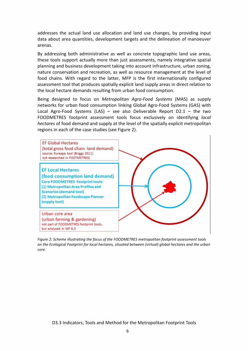
Being designed to focus on Metropolitan Agro-Food Systems (MAS) as supply networks for urban food consumption linking Global Agro-Food Systems (GAS) with Local Agro-Food Systems (LAS) – see also Deliverable Report D2.1 – the two FOODMETRES footprint assessment tools focus exclusively on identifying local hectares of food demand and supply at the level of the spatially explicit metropolitan regions in each of the case studies (see Figure 2).

Figure 2: Scheme illustrating the focus of the FOODMETRES metropolitan footprint assessment tools on the Ecological Footprint for local hectares, situated between (virtual) global hectares and the urban core.


7

2 Footprint basics: demand and supply 2.1 Analysis of demand

Food demand and supply are the two key dimensions of the FOODMETRES metropolitan footprint tools. Food demand results from the average feeding habits of the urban population expressed in the dietary energy, protein and fat consumption per person (see Table 2). Typically such data is only available as the national average and not per city. Given the size and biogeographic range of most European countries – France covering North-Atlantic influences, Alpine and the Mediterranean zone being probably the only exception - average figures can be considered as acceptable.

Table 2: dietary energy, protein and fat consumption (2005-2007) (FAO, 2010).

Food habit surveys provide information resulting from the combination between qualitative - what is consumed? – and quantitative - how much is consumed? – aspects of food consumption. It particularly varies according to geographical area and country, economic, social and cultural aspects, population diets, available food items. FAO statistics (FAO, 2010) give a first response to this issue, summarizing and making easily comparable daily consumption for countries all over the world.

The lack of quantitative data on the amount of food demand leads food consumption survey to play a role as their proxy. Daily pro capita food consumptions can be standardized through their conversion in calorie intake, in order to estimate the extension of agricultural area, devoted to a “reference product”, needed to produce calories to satisfy total caloric intake expressed by population, as proposed by Sali et al. (2014). The authors refer in particular to agricultural land dedicated to wheat, since it is usually used in literature as a benchmark product: in 1815 David Ricardo, in his Essay on the influence of a low price of corn on the profits of stock, one of the most important classical economic book, considered it as the “representative product” to build his theory.

Country Case Study area Proteins

[g/person day]

Fats

[g/person day]

Energy

[kcal/person day]

Kenya Nairobi 58 47 2,060

Slovenia Ljubljana 101 121 3,220

Netherlands Rotterdam 105 136 3,243

UK London 104 145 3,442

Germany Berlin 99 143 3,530

Italy Milan 112 156 3,657


8

Table 3: Comparison of different global-hectare demand figures with EFSA data

National figures (ha)

National figures (ha)

Foreign demand (ha)

EFSA figures (ha)

BERLIN Seemüller Wakamiya (eco)Wheat 0.0145 0.0230 0.0150Other cereal 0.0067 0.0070 0.0060Potatoes 0.003 0.0032 0.0010Sugarbeet 0.0082 0.0082 0.0003Oil 0.0010Vegetables 0.002 0.0020 0.0012Fruit 0.0001 0.0033 0.0070Meat/Fodder 0.0623 0.1390 0.053 0.0410Dairy products 0.0855 0.0748 0.0450TOTAL 0.1823 0.2605 0.3135 0.1175

ROTTERDAM Tilburg Study Gerbens-LeenesWheat 0.027 0.002 0.0090Other cereal 0.003 0.003 0.0030Potatoes 0.00068 0.003 0.0010Sugarbeet 0.0058 0.003 0.0010Oil 0.013 0.071 0.0003Vegetables 0.0015 0.005 0.0100Fruit 0.013 0.008 0.0010Meat/Fodder 0.178 0.075 0.03 0.0290Dairy products 0.047 0.0480TOTAL 0.242 0.215 0.2454184 0.102

Milano national ref. 1 national ref. 2Wheat 0.0170Other cereal 0.0010Potatoes 0.0010Sugarbeet 0.0010Oil 0.0210Vegetables 0.0040Fruit 0.0100Meat/Fodder 0.0220Dairy products 0.0433rice 0.0020wine 0.0050TOTAL 0 0 0.1273

London Schmutz (2015) Schmutz (2015) orgWheat 0.00990 0.0140 0.0080Other cereal 0.00660 0.0093 0.0050Potatoes 0.00077 0.0013 0.0010Sugarbeet 0.00113 0.0000 0.0040Oil 0.00134 0.0000 0.0003Vegetables 0.00223 0.0028 0.0020Fruit 0.00286 0.0031 0.0030Meat/Fodder 0.03962 0.0594 0.0390Dairy products 0.04655 0.0698 0.0500TOTAL 0.111 0.1598 0.1123

Ljubljana avan (2015) conv Glavan (2015) ecoWheat 0.0186 0.0322 0.0120Other cereal 0.0033 0.0066 0.0060Potatoes 0.0023 0.0034 0.0010Sugarbeet no no 0.0000Oil 0.0050 no 0.0020Vegetables 0.0042 0.0048 0.0020Fruit 0.0035 0.0117 0.0020Meat/Fodder 0.0762 0.1048 0.0300Dairy products 0.0321 0.0403 0.0680rice no nowine 0.0090 0.0105 0.0030TOTAL 0.1542 0.2143 0.1260


9

The Metropolitan Foodscape Planner tool (MFP) on the other hand, makes use of the national datasets in the ‘Chronic food consumption statistic (EFSA, 2011) to identify the urban food demand for 12 categories of crops/land use, namely: (1) wheat, (2) other cereals, (3) rice, (4) oil crops, (5) pulses, (6) potatoes, (7) sugar beet, (8) vegetables, (9) fruits, (10) wine grapes, (11) food crops and (12) grasslands. Sali et al. (2014) developed a conversion method to arrive at corresponding global hectare demand figures for the 4 European case study areas (see Annex 1). EFSA did not contain consumption data for Slovenia and Nairobi. For Slovenia, national statistics have been consulted to fill the gap.

The EFSA categories developed by Sali et al (2014) needed to be linked to the MFP-supply data deriving from CORINE land cover and the HSMU data sets. In order t to do so we omitted ‘pulses’ due to its only relative significance in terms of overall consumption and used rise and wine grapes only here relevant (Slovenia and Milano). A comparison between national footprint references from different sources and the global hectare figures calculated on the basis of the EFSA figures showed that the latter resulted in substantially hectare figures (see Table 3).

The discrepancy in total global hectare demand figures derives obviously from the different methods EFSA applies to calculating meat/fodder and dairy area demands. But also for other commodity groups, frequent differences can be detected. Since detailed information on the different calculation models have not been accessible, it was not possible to arrive at rationally synchronised demand data. Instead, we decided to fill data gaps with figures from corresponding assessments where ever possible (e.g. in case of Berlin sugar beets and vegetables in the two national references indicated in stronger colours) and as a general rule used the fodder/dairy figures of the conventional footprint assessments.

2.2 Analysis of supply

Food supply can be referred to land use and available agricultural area in a specific territory or in relation to the amount of obtained raw products (quantities or productivity). This does not mean, however, that these productions still remain confined within particular boundaries, as rather food products move in the global market. This condition restricts the possibility to limit food supply to the local sphere, as it is more precisely affected by all the components of commercial balance, from productions and stocks, to imports and exports.

In this project, or at least at this stage, supply analysis does not aim to monitor flows of food and agricultural products – steps that would be certainly made easier by labelling and traceability systems particularly efficient – but rather to assess and indicate the productive potential of a metropolitan region and its sub-areas, suggesting the extent to which a specific territorial unit can satisfy its needs and potentially those of its close areas.


10

2.3 Building upon existing footprint tools

The Dutch research project SUSMETRO on the impact assessment of food consumption on the sustainability of metropolitan regions (Wascher et al. 2010), demonstrated how regional data can be used to provide policy relevant data for food planning. In the Netherlands, multiple landscape functions such as recreation, cultural identity, ecological resilience and healthy agricultural products – to name just an important few – are under severe pressure by fierce competition against export-driven, industrial forms of agriculture as well as against other potent economic sectors such as urban sprawl, infrastructure and energy (Pedroli et al. 2007; Jaeger et al. 2010).

The Ecological Footprint for a particular population is defined as; “the total area of productive land and water ecosystems required to produce the resources that the population consumes and assimilate the wastes that production produces, wherever on Earth that land and water may be located” (Rees, 2000).

Based on the D2.1 contributions on food governance by Zasada et al. (2013), Corsi et al (2013), and Wascher & van Eupen (2013) we have developed an approach to delineate metropolitan foodsheds. Taken the food demand of a city into consideration, the required amount and location of ‘local hectares’ of agricultural areas meeting these demands are identified as the starting point illustrating the challenge of feeding an urban population on the basis of the potential metropolitan food basket. Drawing from this important background information for explaining the challenge of feeding an urban population, our approach contrasts the food demand with the regional supply as a function of the specific site and farming conditions, showing the food provision capability inside the metropolitan system.

Though global hectares are not of direct relevance for the essential functions of the MFT, we consider them – as mentioned above – as valid references for placing the concrete land demands resulting from food consumption into a wider spatial context. In the following we shall briefly describe the different tool outputs before presenting the MFT methodology.

2.3.1 The European Ecological Footprint Tool EUREAPA contains baseline data on the economy, greenhouse gas emissions, ecological footprints and water footprints for every EU member state and 16 other countries and regions of the world. At the heart of EUREAPA is an environmentally extended multi-region input-output model which combines tables from national economic accounts and trade statistics with data from environmental and footprint accounts.

The model uses The Global Trade, Assistance, and Production project 7 (GTAP7) as its data source. It has the most extensive regional coverage and is a well-recognized database that has been used extensively for trade analysis, agricultural economics and tariff issues, and recently also for carbon footprint analysis. The extensive data system models the flow of goods and services between 43 countries and regions


11

covering the global economy for 130 individual sectors over a year. The sectors cover a range from agricultural and manufacturing industries to transport, recreational, health and financial services. Supplemented with detailed carbon, ecological and water footprint data for hundreds of individual materials and products, EUREAPA can account for the full supply chain impacts associated with the food people eat, the clothes they buy, the products they consume or the way they travel.

This allows the user (e.g. national and EU policy-makers, and those who advise them) to look at the impacts of consumption activities in the context of lifestyles or national differences.

Figure 3: EUREAPA ecological footprint data for food consumption model output for the example of Rotterdam/The Netherlands


12

Table 4: Application of the EUREAPA Footprint Tool (EFT) for the FOODMETRES case study cities, applying the respective population figures as input, adjusted according to a high-urban density index. The columns left show the total household footprint score (EFT total) compared to the footprint resulting from food consumption only (EFT food).

Case Study Population EFT food city +

global hect.

EFT total city +

gh/capita

EFT food city +

gh/capita

London 8,600,000 18,201,393 5.41 2.36

Berlin 3,500,000 7,171,456 5.06 2.05

Milano 1,300,000 2,016,359 3.75 1.55

Rotterdam1 1,300,000 2,875,671 4.87 2.21

Ljubljana 320,000 35,683 3.21 1.04

Nairobi2 2,544,089 2.2 0.8

Note: 1Rotterdam population resembles the Rotterdam City Region which includes adjacent communities (see also figure 3); ²Nairobi calculations have been based on the EUREAPA data for South Africa

2.3.2 The Urban Footprint Tool Based on the average Dutch diet and the average agricultural Dutch production capacity Jansma et al (2012) developed the internet based Urban Footprint Tool (www.stedelijkefoodprint.nl). The authors point out that the tool does not thrive for a high level of quantitative accuracy but has primarily been designed to provide a rough approximation of food consumption impacts at the national level. Operating with global hectares, the tool calculates the surface area needs of any Dutch city on the basis of population figures for the following food groups: vegetables, fruit, potatoes, wheat, sugar, meat, milk and eggs (plus the necessary fodder required to feed the livestock).

The tool has the following characteristics:

1. It is based on the yearly average diet of a Dutch person between 19-30 years in the year 2003.

2. It does not calculate the complete diet, but only the produce that can be cultivated under Dutch circumstances (livestock, horticulture and arable farming). Consumption of exotic products like coffee, fruits and rice are not covered by this tool.

3. It does not take into account the acreage needed to produce the plant based oils in our diet, like soy oil in margarine.

4. It calculates with so called model crops. One model crop symbolizes a certain group of produce. For example: the model crop for the produce group of fruits is apple. Production and consumption data of all other fruits are converted to the production and consumption data of apple.


13

5. It works with average Dutch production data based on conventional agricultural production methods.

6. It functions with processed food that is traced back on one ingredient, like cheese (milk), chips (potato) or bread (grain). Not taken into account are the complex multi-ingredient part of our diet like pizza or cakes.

7. It takes the loss of produce within the food chain (to a certain degree) into account.

8. It takes the necessary concentrate to feed the livestock partly (approximately 60%) into account.

The tool is based on the databases created and described in Jansma et al. (2012) and uses the consumption figures of Hulshof et al. (2004).

Figure 4: User interface output of the Urban Footprint Tool for the city of Rotterdam (600.000 inhabitants).

The tools estimated area demand amounts to only 0.056 global hectares per person. Other sources such as Rood et al. (2004) put forward 0.31 global hectares, the study of Wageningen UR in cooperation with the Brabantse Milieufederatie “How to feed Tilburg” (2009) suggests 0.24 global hectares, while Gerben-Leenes (2002) calculated 0.21 global hectares as a standard reference. Jansma et al. (2013) explain the tool’s underestimation as a result from (1) the selection of mainly locally available food types, and (2) the conversion of imported food to notoriously high Dutch yields.


14

2.4 Conclusions Despite it shortcoming, we found the underlying principles of the Urban Footprint Tool as a valid starting point when developing an internet-based approach towards footprint-based impact assessment. We also felt that absolute accuracy in terms of the resulting per hectare figures cannot be the most important objective when building such a tool. The large variety of methodological approaches on the one hand, and the more abstract notion of many global footprint assessments on the other did not really help to improve our understanding of metropolitan food systems, but quite to the contrary has resulted in the belief that the existing agricultural lands around Europe’s cities will never be able to provide enough food for all citizens. Studies such as ‘How to feed Tilburg’ have demonstrated that a fair amount of the required global hectares is actually available, but is used for other purposes, among it exporting agricultural goods to remote locations. Looking at the existing footprint assessments and reference in the light of a societal debate that seems to be polarised between two utopian world views, namely the grow-it-yourself philosophy of the urban gardening movement and the resource-efficiency paradigm of modern industrial agriculture, we felt that there is need for a Metropolitan Footprint Tool that allows users to detect the concrete locations and the available amounts of suitable farmland (supply) in relation to urban consumption needs for the most essential food groups on the basis of urban population figures (demand). When pursuing such a goal, we have been of course aware of the fact that the high density of cities in many of Europe’s poly-centric regions will pose major challenges to a region-based food supply. At the same time, our research has demonstrated that both the available land resources and food chain innovation – e.g. the large capacities of greenhouse complexes in the Rotterdam metropolitan region, not to mention the prospects of departing from a protein-based diets – are pointing at a wide range of opportunities to largely increase the proportion of regional food supply with many positive synergy effects for local economies, environmental conditions and societal cohesion – in short: for sustainability.

Nearly three of a quarter of the land is needed to produce the animal based protein in our diet. Jansma et al. (2012) argue that more of the daily food basket could be produced locally if consumers behaviour changes towards less meat consumption and more in season products.

3 Metropolitan footprint tools 3.1 Introduction

Within the debate of urban resilience and metabolism, reduction of ecological footprint and self-sufficiency, regionalized food systems and shortening of supply chains have gained increasing importance. Manifold benefits, such as reduction of vulnerability against crisis situation of the global food supply, more efficient energy


15

and resource use or social welfare and competitiveness of the regional food sector, have encouraged many metropolitan jurisdictions to develop food policies, aiming at fostering local food systems and reconnecting cities with their foodsheds. As a precondition to policy making, analytical models are required, which determine the spatial extent of surrounding farmlands necessary to provide sufficient food, respectively the regional food balance between production and consumption.

The objective to spatially analyze the footprint of metropolitan food supply implies two specific challenges, which require the application of different methodological approaches – (i) The analysis of the spatial extent of the agricultural area required for food production (“How much?”); and (ii) the distribution of the various land use types, which are required for food production (“Where”?). Both modeling approaches feature not only methodological differences, but also in terms of input data, modeling rational and the degree of stakeholder interaction. However, both models apply a common spatial understanding of minimizing the distance of food production and consumption location (urban core), resulting in an idealized circular representation of food zones, comparable to the renowned model by Heinrich von Thünen (1826) about the spatial distribution of agricultural commodities as a function of transportation cost to the central market.

In the FOODMETRES approach, the question of the area demand for food supply is addressed by the Metropolitan Area Profile and Scenario (MAPS) tool, which adopts a straightforward data-driven approach of connecting regional food demand (local hectares) with the regional area productivity. Its main strengths are (1) the spatial representation (mapping approach), (2) the differentiation of commodity types, (3) the ability to apply different food production (e.g. organic farming, food loss) and consumption (e.g. vegetarian, healthy diets) or population scenarios, and (4) the analysis of theoretical self-sufficiency levels. The Metropolitan Foodscape Planner (MFP), at the contrary, offers (1) hands-on impact assessment tool for balancing commodity surpluses and deficits, (2) a visual interface that depicts food zones to make impacts spatially explicit, (3) landscape-ecological allocation rules to base land use decisions on sustainable principles, and (4) European data such as EFSA, LANMAP, HSMU and CORINE Land Cover to allow future top-down tool applications for all metropolitan regions throughout the EU.


16

Figure 5: Data and reference environment of the metropolitan footprint tools MAPS (Zasada et al. 2014) and MFP (Wascher & Jeurissen, 2015).

3.2 Metropolitan Area Profile and Scenario (MAPS) tool

Focussing at the spatial extent of the footprint of food production, the Metropolitan Area Profile and Scenario (MAPS) tool represents a spatial model which takes both parameters of regional yields and diets into consideration, broken down to a set of commodity groups. This allows the model’s sensitivity regarding alternative agricultural systems (conventional and organic), reduction of food loss and waste, different diets (given and health recommendations) and temperate domestic and necessary global production. The model has been applied in the five European metropolitan regions London, Berlin, Milan, Rotterdam and Ljubljana as well as for the Nairobi, Kenya. It is the main objective of the MAPS tool to develop an easy-to-adopt approach to spatially assess the necessary agricultural area to supply a pre-defined city, metropolitan area or region. It further should allow for comparative assessments of area demand for food production (based on regionalized agricultural production, diets and population data), scenario analysis of effects of organic, healthy or vegetarian diet change, prevention of food waste and loss and the regional self-sufficiency.


17

3.2.1 Modelling Procedure and Database Food supply

The analysis of the food supply is based on actual regional agricultural conditions depending on climatic and bio-physical conditions, such as soil fertility, resulting in differences in crop yields. Therefore average values for the different commodity types are taken from agricultural statistics, mainly from regional databases, complemented by national and international figures (Statistik Berlin-Brandenburg 2012, AGRIISTAT 2012, DEFRA 2013, EUROSTAT 2012, Slovenia Statistical Office, FAO Food Balance Sheets). For crops, which cannot produced locally, such as exotic fruits, cacao, tea, coffee, etc. global yield values from FAO statistics are taken into consideration.

Livestock production

The modelling of the livestock production and fodder demand represent a specific challenge when assessing the area demand for food supply. Especially as various fodder production (on arable land) and grazing regimes are applicable, our modelling approach draws on existing area demand estimations by Woitowitz (2007) and Wakamiya (2010) for European livestock systems as well as Bouman et al. (2005) for an extension for Kenya.

Final product conversion

During the processing of food, especially in livestock production (e.g. meat, milk, eggs), but also for arable crops and fruits (e.g. sugar, cereals, fruits, beverages), there is a significant weight loss during the conversion process from the agricultural production (e.g. slaughter weight, raw milk) to the final production (etc. egg mass, edible sugar, milk, butter, cream, cheese), which is also included in the modelling exercise. Table 5 provides an overview of the specific commodity (groups) used in the model, their regional yields (for the example of Berlin-Brandenburg region) and the required agricultural areas per kg final product.

Conventional vs. organic production

As an example of different agricultural production intensities, we have differentiated conventional production (reference system) and organic production. Therefore, the meta-analysis of Posinio et al. (2014), who have reviewed and interpreted a high number of empirical studies on yield differences between conventional and organic production. The authors found a range from in average lower yields of 19.2% to 8.5% (with multi-cropping and crop rotation) to conventional production.


18

Figure 6: Demand analysis for the case study area Berlin-Brandenburg as developed for MAPS (Zasada, 2014).

Food demand

The food demand is determined by the quantity of the regional population as well as average food consumption patterns (diets), which are also characterised by substantial differences, e.g. between countries or urban and rural areas (see Gerbens-Leenes & Nonhebel (2002)). To allow comparability between the case study regions, we applied the food balance database of the FAO (http://faostat3.fao.org/download/FB/CC/E), which covers all six regions. The basic per capita values (see Table 5 for the example of Berlin-Brandenburg region) is then projected for the overall regional population for the reference situation (conventional production, current food consumption and food losses and waste levels.). This will be used as starting point for the application of different scenarios of population change, food consumption, food loss and waste as well as different production intensities.


19

Table 5: Food consumption and production per commodity (group), Example Berlin-Brandenburg region.

Commodity (group) Consumption, in kg/capita/year (2011)

Yields, in t per ha, conventional (2006-10)

Agricultural area demand in m²/per kg final product

Laying hens (eggs) 12.75 2.08 4.80 Poultry meat 17.97 2.22 4.50 Pig meat 53.48 1.41 7.10 Fish meat (from farmed fish) 4.41 1.43 7.00 Milk for dairy products 309.90 6.25 1.60 Beef cattle 13.37 0.74 13.60 Other meat (goat and sheep) 0.88 1.00 10.00 Cereals (flour, bread & other cereal products, beer) 124.21 5.00 2.00 Oilseeds (vegetable fat) 11.57 3.20 3.13 Potatoes & Sweet Potatoes 111.66 30.00 0.33 Sugar (sugar beet, sugar cane) 39.31 50.00 0.20 Tomato 7.03 250.00 0.04 Vegetable, other 58.67 28.86 0.35 Roots & Tuber (Asparagus, carrots, turnips, etc.) 22.33 40.00 0.25 Pulses (beans, peas, others) 1.01 5.57 1.80 Onion 4.17 20.00 0.50 Apples 43.22 20.00 0.50 Fruits, other (temperate regions) 29.96 7.12 1.40 Grapes 6.32 10.00 1.00 Citrus Fruit and other tropical fruit 18.45 9.39 1.06 Banana 8.00 20.42 0.49 Olives 0.06 2.00 5.00 Nuts (treenuts, groundnuts, coconuts) 8.26 1.00 10.00 Cacao 2.34 0.48 20.83 Tea 0.14 2.30 4.35 Coffee 4.57 0.84 11.90 Wine 24.68 3.50 2.86

Food losses and waste

As significant contribution to food demand, the MAPS model takes the losses and waste into consideration. According to the Food and Agriculture Organisation (FAO) these losses and wastes sum up to about one third of the edible parts of food produced for human consumption, which is roughly 1.3 billion ton per year at the global scale. Consumers in Europe and North-America alone waste between 95-115 kg/year, while it is way lower in sub-Saharan Africa and South and Southeast Asia (6-11 kg/year) (FAO 2011). However, food is also lost within the whole food supply chain, including (1) Agricultural production; (2) Post-harvest handling; (3) Processing and packaging; (4) Retail and distribution; (5) Households and catering (FAO, 2011) (see Table 6). At each of the single steps a certain share of the food gets lost, avoidable and unavoidable, increasing the demand in total. By implication, food losses and waste represent the potential to reduce the food demand and therewith the agricultural area demand. There are a number of studies which aim at


20

quantifying these shares at national, European or global scale (FAO, 2011; European Commission, 2010). In our modelling exercise, we referred to the figure of the FAO (2011) as well as Buzby and Nyman (2012). These are translated into area factors.

Table 6: Food losses and waste at the different steps of the food supply chain

Food Chain Step Explanation of Food Losses and Waste

Food losses in agricultural production

Mechanical damage and/or spillage during harvest operation (e.g. threshing or fruit picking); for bovine, pork and poultry meat, losses refer to animal death during breeding. For fish, losses refer to discards during fishing. For milk, losses refer to decreased milk production due to dairy cow sickness (mastitis).

Postharvest handling and storage

Spillage and degradation during handling, storage and transportation between farm and distribution

Processing

Spillage and degradation during industrial or domestic processing, e.g. juice production, canning and bread baking. Crops are sorted out if not suitable to process or during washing, peeling, slicing and boiling or during process interruptions and accidental spillage

Retail and Distribution

Losses and waste in the market system, at e.g. wholesale markets, supermarkets, retailers and wet markets

Household and catering

Losses include avoidable (uneaten food, losses through cooking) and unavoidable (non-edible margins) of the food and drinks consumed in households and away from home

3.2.2 Spatial modeling Starting point for the spatial modelling is the aggregated agricultural area required for food supply. This area is represented by a circle with a centre point (centroid) of the polygon of the administrative boundary. Subsequently, the radius of the circle is calculated as

(1) r=�(𝐹𝐹𝐴𝐴

+ 𝑇𝑇 − 𝐴𝑇)/𝜋

,with FD (Area required for local food demand), AR (Share of agricultural area (of the region)), LT (Total area (of municipality)) and AL (Agricultural area (of municipality)). Here, the spatial model takes the available agricultural area within the municipality (AL) and the surrounding region (AR) into consideration.

3.2.3 MAPS Application The MAPS model has been applied to the situation of the five European metropolitan regions included in the FOODMETRES project (London, Berlin, Milan, Ljubljana and Rotterdam), which are characterised by population sizes of the urban core and population densities and availability of the overall region. Therefore, population and land use statistics for the local jurisdictions of all regions have been compiled. The CSRs cover a broad diversity of regional situations, with regional population sizes between 2.1 Mio (Slovenia) and 22.7 Mio (London, South-East & East England) as well as different availability of agricultural area between 32.9 and 69.4% (see Tab. 7).


21

Table 7. Population and agricultural area.

Case Study Regions

Core city Berlin London Milan Ljubljana Rotterdam

Administrative region Berlin & Brandenburg

London, South-East & East England

Lombardy Slovenia South Holland City Region

Population core city 2015, in tsd. Inh. 3,502 8,174. 1,242 280 1,209

Population region 2015, in tsd. Inh. 6,037 22,656 7,885 2,053 3,695

Total area, in km² 30,53 38,260 13,111 20,274 2,819

Utilisable Agricultural Area (UAA), in km² 14,576 26,566 4,892 6,663 1,685

Share UAA, in % 47.7 69.4 37.3 32.9 59.8

The five resulting spatial representation of the area demand of the urban core (solid line, bold), local jurisdictions (solid line, thin) and the overall region (dashed line) in the reference scenario (population 2015; average consumption pattern including food waste & loss; Conventional production) are shown in figure 7 and table 7. The spatial extends of the required agricultural area show very different pattern, corresponding to food consumption, population and land use in the individual CSRs.

In the Berlin case 6,827 km² for the city of Berlin or 11,770 km² for the region Berlin-Brandenburg is required. So despite the poor soil conditions (most or the rural area is designated as less favoured area), both city and regions can theoretically supply itself within their own boundaries, as the total farmland cover an area of about 13,230 km² (2012). Especially the relative low population density (and the related low food demand) of the surrounding region mitigates particular food stress.

The London case is characterised by a high demand for food from the urban core as well as other major cities in the region, resulting in an area demand of 13,989 km² (London) and 38,773 km² (London, South-East & East England). Despite high agricultural area share with more than 26,500 km² farmland, the demand clearly exceeds the regional self-sufficiency potential by nearly 50%. Particularly due to the high population density in the direct vicinity of London as well as the area constraints of the footprint area of the British Midlands and the island location, serious food stress can be considered.

The competition between the core city (Rotterdam) and surrounding region (South Holland) is even more pronounced in the Dutch case. Despite a farmland share of 60% (1,684 km²) and an area demand of 1,133 km² for Rotterdam, the regional demand of 6,713 km² overdraw the regional potential four times. A compensation of the resulting food stress from neighbouring regions can also not be expected (high population density in the Netherlands, Belgium and Northern France, which is already belonging to the Paris footprint area as well as the coastal location).


22

Figure 7: Area demand conventional food production for Berlin (upper left), London (upper right), Ljubljana (middle right), Rotterdam (middle left) and Milan (lower left). Inner circle: area demand central city; Outer circle: area demand region. Based on population figures 2012. Source: Zasada et al. unpublished. Note: Both MAPS have different geographical scales.


23

Due to low population numbers and density in the case of Ljubljana (urban core and surrounding area, the Slovenian situation rather depicts a situation with full regional self-sufficiency. The regional 6,663 km² of agricultural land is sufficient to cover the demand of 583 km² (urban core) and 4,269 km² (region). However, also here some physical constraints of the near Alps Mountains need to be taken into consideration.

Also the Lombardy metropolitan region is characterised by a mountainous situation in the North and agricultural plains in the South of the region. In addition a small-scale administrative structure is noticeable. Whereas the area demand for food production of the city of Milano (2,548 km²) can be covered by the surrounding region (4,892 km²), the demand from the regional population (16,178 km²) is more than three times higher than the regional available farmland.

3.2.4 Metropolitan Self-sufficiency Another application of the MAPS tool is the analysis of the local and regional self-sufficiency level (SSL), i.e. the percentage ratio between supply and demand expressing the extent of a territorial unit to meet its own food requirements. The analysis of the spatial distribution for each individual locality provides indications about their food self-sustainability and the possibility to satisfy urban demand through proximity agriculture. It gives therefore indications of local hotspots of possible future food stresses. Figure 8 provides an overview of the SSLs in the CSRs. Values of 100% (green colour) and more indicate theoretical self-sufficiency in the respective area, whereas jurisdictions with values lower than 100% (red colour) cannot be supplied from their own territory and require “import” from outside. Regional differences regarding the spatial distribution of SSL is illustrated by the frequency of SSL class occurrence in figure 8.

Figure 8: Self-sufficiency level: Frequency distribution of municipalities in the five case study regions.

0%

10%

20%

30%

40%

50%

60%

70%

80%

90%

100%

Berlin Ljubljana London Milan Rotterdam

>1,000 %

500-1,000 %

250-500 %

200-250 %

150-200 %

100-150 %

75-100 %

50-75 %

25-50 %

10-25 %

5-10 %

<5 %


24

Figure 9: Self-sufficiency level at municipality level for Berlin (upper left), London (upper right), Ljubljana (middle right), Rotterdam (middle left) and Milan (lower left). Red colour indicates under-supply, green colour over-supply. Based on population figures 2012. Source: Zasada et al. unpublished. Note: Both MAPS have different geographical scales.


25

The mono-centric Berlin-Brandenburg region is characterised by a by a concentration of municipalities which show undersupply of farmland for the city of Berlin and its direct adjacency, whereas large parts of the peripheral rural areas can realise significant food production surpluses, being able to “export” to food stress areas. Whereas also in the London region, the core city faces a strong food deficit, the majority of urban places can be easily supplied by the near surrounding, which show SSL of 100% and more. However, the absolute area demand through the high population number results in an undersupply at regional level. In the majority of municipalities in the South Holland region (Rotterdam) are characterised by SSL of below 100%, often even not exceeding 25% and below, so that a rather continuous food stress can be expected in the region. Similarly, but less pronounced is the food stress situation of Milan and the Lombardy region, with a majority of municipalities without theoretical self-sufficiency. However, the specific of the Lombardian administrative structure deserves attention, which is characterised by many urbanised communities with a small territory on the one side and large rural communities on the other. In contrast, nearly 90% of the Slovenian municipalities provide a full local self-sufficiency level of 100%. Moreover, a majority provide more than 200% of the required farmland within the own boundaries. Only Ljubljana as the urban core and some major cities face local undersupply.

Table 8: Exemplary scenarios applied in with the MAPS-tool.

Scenario Description

S1 2015 Conventional, all commodities, incl. food waste & loss (Reference) S2 2015 Conventional, domestic production, incl. food waste & loss S3 2015 Conventional, domestic production, without household food waste S4 2015 Conventional, domestic production, without household food waste & loss S5 2015 Organic min, all commodities, incl. food waste & loss S6 2015 Organic min., domestic production, incl. food waste & loss S7 2015 Organic min., domestic production, without household food waste S8 2015 Organic min., domestic production, without household food waste & loss S9 2015 Organic max., all commodities, incl. food waste & loss S10 2015 Organic max., domestic production, incl. food waste & loss S11 2015 Organic max., domestic production, without household food waste S12 2015 Organic max., domestic production, without household food waste & loss

3.2.5 Scenario Application As one of the main objectives of the MAPS tool, various food demand-supply scenarios can be applied to the reference situation. These scenario settings can include variations of the agricultural production system and intensity, such as extensive production, organic farming, intensive greenhouse production or forms of sustainable intensification. Moreover, potentials through the reduction of food losses and waste as well as consideration of regional cultivation traditions can be included. At the demand side, scenario elements can encompass changing (future) population numbers or changing diets, e.g. to estimate impacts of changing population composition (i.e. new dietary cultures through in-migration) or changing


26

eating behaviours and trends (i.e. seasonality, healthy, vegetarian or vegan diets). Table 8 gives an overview of 12 scenarios, which have been applied in the FOODMETRES project.

Figure 10: Agricultural area demand per capita in different case study region, in hectare.

In the scenario situations, first of all the agricultural area demand per capita is variable. These changes occur similarly throughout all CSRs into the same direction, even though with different amplitudes. Particularly impacts of food loss and waste reduction (S3, S4) as well as of conversion of production towards organic farming (S5) are clearly depicted. However, the scenarios also show the potential of certain organic systems (S9) or the combinations with food loss and waste reduction (S7, S8, S11, S12) to have a reduced area impact (see Tab. 9).

The aggregated agricultural area demand for all CSRs is presented in Tab. 9. It can be noticed, that with the exception of Nairobi (1,243 m² in scenario 1), all per capita area demand differ only marginally (Berlin: 1,950 m², London: 1,711 m², Milan: 2,052 m² Ljubljana: 2,080 m², Rotterdam: 1,817 m²). Whereas a similar pattern between the CSRs can be observed, also here Nairobi plays a special role, at its footprint responds less sensitive to the given parameter changes (food loss and waste as well as organic farming).


27

Table 9. Aggregated agricultural area demand per case study region and scenario, in km².

Case Study Region

Scenario Berlin London Milano Ljubljana Rotterdam

S1 Core city 6,827 13,989 2,548 583 1,133 (Region) (11,770) (38,773) (16,178) (4,269) (6,713)

S2 Core city 5,661 11,887 2,224 491 969 (Region) (9,760) (32,946) (14,115) (3,598) (5,741)











3.3 Metropolitan Foodscape Planner (MFP) supply tool

3.3.1 Data and indicators Building the Metropolitan Foodscape Planner tool (MFP) requires a series of data management and GIS operations to be performed in Excel and Arc-Info. Using the example of the Rotterdam Metropolitan Region procedure, we will illustrate the following sequence of steps that are required:

- Creating the dynamic footprint-driven spatial zoning framework (von Thünen);

- Disaggregation of the CORINE land cover units to arrive at distinctive land use types in form of commodity groups (HSMU);


28

- Establishing commodity group allocation rules on the basis of landscape units (LANMAP);

Configuration of the digital MAPTABLE to allow hands-on impact assessment for stakeholders when engaging in serious gaming to balance commodity surpluses and deficits in MFP-zones.

In combination, MFP allows users to detect concrete spatial locations and the available amounts of suitable farmland (supply) around cities for the most essential food groups on the basis of urban population figures (demand). Other than MAPS, MFP is a dynamic tool in the sense that users can directly undertake – by drawing with a pen on a digital table – land use changes in response to the footprint assessments which are provided by a geographic information system. MFP allows the spatial allocation up to 2 food groups (depending on the respective case) making use of the European data sets shown in Tab. 10.

Table 10: Data Layers applied in the MFP model.

Data Layer Source Cities_startpoint_Berlin

Corine Land Cover 2006

http://www.eea.europa.eu/data-and-maps/data/corine-land-cover-2006-raster-3 version 8 april 2014, download 13 jan 2015 in arccat export .tiff als esrigrid in MFT.gdb

Natura2000

http://www.eea.europa.eu/data-and-maps/data/natura-5#tab-gis-data shapefile Natura2000_end2013_rev1.shp

Lanmap2v1

European Landscape Typology LANMAP (Mücher et al. 2006) lanmap2_v1_level_4_ls-cod

Multi-ring-buffer around city_startpoint: first calculate radii based on:

combine distance-raster and 3 rasters with the correct legenda and greyed areas total demand per ring

HSMU

Homogenous Soil Mapping Units (HSMU) as modelled by CAPRI (Kempen et al. 2005) and Eurostat crop area data desaggregated to hsmu’s by CAPRI. Year per country: NL 2008, BL 2008, DE 2008, PL 2004.

Though less accurate as the national land use survey data, HSMU is available for the whole of Europe, allowing direct top-down assessments without resource-consuming data gathering procedures. The concept of spatially allocating specific food groups for which a certain supply deficit has been recognised – e.g. vegetables or oil seeds are typically underrepresented in the metropolitan surroundings of cities – to areas with clear food supply surplus coverage, for example grasslands, points at the need to guide such stakeholder decisions by offering additional land use related references. MFP is doing so by the means of two support mechanisms:

http://www.eea.europa.eu/data-and-maps/data/corine-land-cover-2006-raster-3

http://www.eea.europa.eu/data-and-maps/data/corine-land-cover-2006-raster-3

http://www.eea.europa.eu/data-and-maps/data/natura-5#tab-gis-data

http://www.eea.europa.eu/data-and-maps/data/natura-5#tab-gis-data


29

- a metropolitan zoning concept that suggests an agreed-upon sequence of food-zones following each other inspired by von Thünen (1826);

- a series of food group allocation rules specifically designed for each metropolitan region on the basis of landscape-ecological references (LANMAP)

3.3.2 The MFP spatial zoning framework Building upon the classical market-centered von Thünen (1826) model, but translating it into contemporary agri-environmental and spatial planning strategies, we developed the following concept of metropolitan zones: (1) urban core area, followed by (2) a green buffer reserved for nature and recreation, (3) a metropolitan food production zone differentiating a plant-based and a protein-based supply zone, and (4) a transition zone which is meant to provide food also for adjacent urban areas.

Making use of the figures for urban food demand, MFP projects the corresponding land demand figures in the form of ‘local hectares’ to those areas of land that can be considered to be eligible for farming. We hence excluded all land covered by urban areas, waterbodies (sea, lakes & rivers), nature and landscape conservation sites, forests and other non-farmlands such as rocks, beaches and swamps. Around urban centers we reserved a zone as ‘green buffer’ for mainly biodiversity and recreational functions – but without investing into further elaborations. Here we obviously consider all land to primary serve this potential function. The guiding principle for introducing such a green buffer was based on the assumption, that (1) urban dwellers will appreciate short travel distances to enjoy these functions, and (2) there is a basic need to offer micro-climatic compensation for high density urban zones in terms of air quality and circulation.


30

Figure 11: The von Thünen model in two variation – as isolated state and a modification displaying river access and a sub-centre location.

Following the green buffer, we gave full priority to the supply with plant-based food groups such as rotation crops (wheat, sugar beet, potatoes), other cereals, oil seeds, vegetables and fruit, taking the total hectare requirements for calculating the width of the plant-based metropolitan food-ring, as we call it. This means that the amount of available farmland within this ring matches exactly the total amount for land needed for all plant-based food groups, but that actual distribution of these food groups within this ring shows of course large deficits and surpluses, thus the type of expected imbalance we consider as an important reference when exploring potentials for optimizing the supply with regional food on the basis of the available land. Directly following the plant-based ring, follows the protein-based food production ring which extension corresponds exactly to the amount of hectares requires for fodder crops and dairy farming. The decision to place livestock farming at a remote position follows the need to reduce direct expose of core urban population to this sector’s impacts (health, odors, food safety issues).

Figure 11 shows the von Thünen model in two variations with market gardening and milk production in the direct periphery of the central city. This corresponds in the MFP approach with the concept of the urban agriculture as part of the central core area and extensive dairy farming at the fringe and in the green buffer. Not being part of the agro-food sector, firewood and lumber production has not been taken up in the scheme. Crop farming and three-field system corresponds with the plant- based food ring, so does the location of livestock farming at the outer periphery in line with the MFP’s zoning concept.

In the following we explain the step-wise approach towards building the MFP zoning framework for Rotterdam:


31

Green buffer

Determining the green buffer is the only step that is not driven by the ecological footprint data derived from EFSA/national data. This is because the area demand for recreation and nature experience is not considered to be directly related to matters of food consumption. At the same time research has shown that urban dwellers benefit from a certain minimum of available open green space to compensate for urban density, noise and pollution. However, technical references differ quite largely and given the fact that the urban buffer is not the only space offered preserved for nature and recreation – all existing protected areas, forests and water bodies are exempt from food planning objectives – we decided to establish a certain minimum distance as the rule of thumb: namely 50% of the urban core’s average radius between its periphery and the subsequent metropolitan food rings dominated by high agricultural production.

Figure 12: MFP output for the metropolitan region of the Rotterdam City Region.

For Rotterdam the radius of the Urban Core is 10km (Figure 12). For the Green Buffer half that distance – thus 5 km – has been taken. Within this Green Buffer we did not consider existing land use areas to be eligible for land use change/food group allocation plans. We did though consider to maintain existing grasslands to contribute to extensive livestock farming as in the past. Remaining areas are meant to be successively converted to extensive cultural landscapes, nature areas and recreational parks.


32

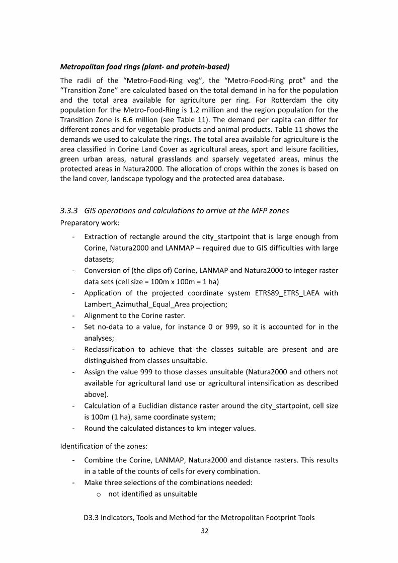
Metropolitan food rings (plant- and protein-based)

The radii of the “Metro-Food-Ring veg”, the “Metro-Food-Ring prot” and the “Transition Zone” are calculated based on the total demand in ha for the population and the total area available for agriculture per ring. For Rotterdam the city population for the Metro-Food-Ring is 1.2 million and the region population for the Transition Zone is 6.6 million (see Table 11). The demand per capita can differ for different zones and for vegetable products and animal products. Table 11 shows the demands we used to calculate the rings. The total area available for agriculture is the area classified in Corine Land Cover as agricultural areas, sport and leisure facilities, green urban areas, natural grasslands and sparsely vegetated areas, minus the protected areas in Natura2000. The allocation of crops within the zones is based on the land cover, landscape typology and the protected area database.

3.3.3 GIS operations and calculations to arrive at the MFP zones Preparatory work:

- Extraction of rectangle around the city_startpoint that is large enough from Corine, Natura2000 and LANMAP – required due to GIS difficulties with large datasets;

- Conversion of (the clips of) Corine, LANMAP and Natura2000 to integer raster data sets (cell size = 100m x 100m = 1 ha)

- Application of the projected coordinate system ETRS89_ETRS_LAEA with Lambert_Azimuthal_Equal_Area projection;

- Alignment to the Corine raster. - Set no-data to a value, for instance 0 or 999, so it is accounted for in the

analyses; - Reclassification to achieve that the classes suitable are present and are

distinguished from classes unsuitable. - Assign the value 999 to those classes unsuitable (Natura2000 and others not

available for agricultural land use or agricultural intensification as described above).

- Calculation of a Euclidian distance raster around the city_startpoint, cell size is 100m (1 ha), same coordinate system;

- Round the calculated distances to km integer values.

Identification of the zones:

- Combine the Corine, LANMAP, Natura2000 and distance rasters. This results in a table of the counts of cells for every combination.

- Make three selections of the combinations needed: o not identified as unsuitable


33

o not identified as grasslands and not as unsuitable (= in fact all areas suitable for cropland farming)

o all grasslands irrespective of protection - For each selection: calculation of the area available for production within

each km distance. (“Grasslands” contains the Corine Land Cover classes pastures and natural grasslands)

The size of the rings necessary for the demand can be deduced from this in the way described below.

1. Calculate the area needed for the “Metro-Food-Ring veg” as the city population times the demand factor for conventional vegetable production. The size of the “Metro-Food-Ring veg” can now be derived from the “not grass and not unsuitable” table above.

2. From the “grasslands irrespective of protection” table above derive the area available for grassland in the Urban Core and Green Buffer irrespective of the Natura2000 protection. Divide this with the demand factor for ecological animal production to get the number of people provided with ecological animal products from the Urban Core and Green Buffer.

3. Subtract this number from the total city population and use the result to calculate the area needed for the “Metro-Food-Ring prot” by using the demand factor for conventional animal production.

4. Calculate the area needed for the “Transition Zone” based on the region population and the demand factor for ecological production (both vegetable and animal products).

Calculate a Multi-ring-buffer around the city_startpoint with these radii, the zones.

Table 11: Calculations for the MFP zoning distances for the City Region and OECD Region of Rotterdam.

Ring types (zones) Distance (km)

Surface area of rings (ha) Demand factor (ha/p) Population

Arable or grass

Arable Grass (includ. protected)

Arable or grass

Arable Grass-land

surface (ha)

land use type

Rotterdam city region 1,200,000 Rotterdam OECD region 7,800,000 Urban Core 0-10 12642Green Buffer 10-15 25608Organic dairy in UC & GB 0-15 38250 14,436 0.05 288,720 grass, irrespective

of protectionMetro-Food-Ring (plant-based)

15-24 68930 41,129 0.0341 1,200,000 40,920 arable, not protected

Metro-Food-Ring (protein-based)

24-40 163,445 0.178 911,280 162,208 arable and grass, not protected

Transition-Zone 40-150 1,402,085 0.2121 6,600,000 1,399,860 arable and grass, not protected

Required surface area (population x demand factor)


34

3.3.4 Land cover disaggregation towards HSMU commodity groups The crop data per HSMU comes in *.gdx format. The approach was as follows:

- Calculate per HSMU the area for each crop category according to the crop category table, both absolute and relative to the total HSMU area (= density). Also determine the dominant crop (qua area).

- Join these data to the HSMU geometry. - Make a selection of the HSMU’s with crop data, and extract the HSMU’s

within the outer zone boundary. - Union the above with the zones (rings) defined previously and aggregate

based on the zone-id and HSMU-ID. If the zones cross national borders combine the HSMU data of those countries.

- Calculate for each crop category the absolute value of the area in that HSMU polygon in that zone in ha as: percentage crop area multiplied with the HSMU polygon area in ha.

- Calculate the total area per zone for each crop category. - Calculate for each zone the division of area’s between the crop categories.

Base the calculation of the “Status quo” of crop area per zone and per crop type on these divisions.

- Comparison of the status quo with the demand results in the surplus/deficit.

Table 12: Breakdown of supply and demand based on CORINE LC – HSMU disaggregation for all three MFP-rings of Rotterdam City Region & OECDE region.

Method validation

Making use of the European HSMU datasets introduces high levels of data aggregation to our method. We hence were interested to run a validation of the results by comparing with national land use data at higher resolution and accuracy. The corresponding most recent Dutch land cover map is LGN (Landgebruik Nederland) version 7 (LGN7) which we re-classified for the selected area in Rotterdam within a 40km radius from the urban city central point (up to the boundary of the Metro-Food-Ring protein). The re-classification was necessary to ensure that we reach a high level of comparability with the HSMU-approach.

Population 1,200,000 911,280 6,600,000

Zone Metro-Food-Ring veg Metro-Food-Ring proteine Transition ZoneFood groups Ha/capita Demand

(ha)Supply (ha)

Surplus/Deficit (ha)

Ha/capita Demand (ha)

Supply (ha)


Ha/capita Demand (ha)

Supply (ha)


Crop rotation 0.0163 19,560 18,794 -766 0 35,677 35,677 0.0163 107,580 309,528 201,948Other cereals 0.0030 3,600 1,396 -2,204 0 5,844 5,844 0.0030 19,800 113,597 93,797Oilseedplants 0.0003 360 105 -255 0 600 600 0.0003 1,980 4,678 2,698Fodder 0 5,920 5,920 0.1280 116,644 18,664 -97,980 0.1280 844,800 372,776 -472,024Vegetables 0.0015 1,800 4,984 3,184 0 20,207 20,207 0.0015 9,900 59,349 49,449Fruit 0.0130 15,600 526 -15,074 0 1,567 1,567 0.0130 85,800 26,852 -58,948Wine 0 9 9 0 13 13 0 53 53Grassland 0 37,195 37,195 0.0500 45,564 80,873 35,309 0.0500 330,000 515,252 185,252Total 0.0341 40,920 68,930 28,010 0.1780 162,208 163,445 1,237 0.2121 1,399,860 1,402,085 2,225


35

The two largest – in terms of surface area – HSMU-dominant crop types are ‘rotation’ (33%) and grassland (45%). When comparing the landcover areas of the two datasets, we found that 70% of the LGN-grassland matches the HSMU-dominant crop type grassland. And vice-versa, 73% of the HSMU-grassland is also LGN-grassland. In the case of ‘rotation’-crops, 63%, 61% and 64% of LGN-potato, sugar beet and wheat are matching the HSMU-crop type ‘rotation’.

Other crop types do not match 1 to 1 LGN-categories: the HSMU dominant crop-type ‘vegetables’ are mainly corresponding to LGN-potato/sugar beet/wheat (38%); grassland (22%); other crops (15%). HSMU crop type ‘other cereal’ matches LGN-grassland with 36% and forest/nature (also 36%). HSMU crop-type ‘fruit’ is corresponding to LGN-potato/sugar beet/wheat (21%). For detailed information on these validation results please see Annex 1.

This validation exercise demonstrates that using European HSMU-data sets for assessing the spatial distribution of major crop types in Europe goes clearly on the account of accuracy. However, we assume that this inaccuracy is mainly related to locational attributes rather than to absolute crop figures. The latter requires further validation efforts.

3.3.5 MFP-tool configuration of the digital MAPTABLE The MAPTABLE tool consists primarily of a 1000 m by 1000 m grid layer (the Drawing Layer) portraying current dominant crop types, which can be interactively modified by selecting a new crop type and ‘painting’ it on one or more cells. As new crop types are allocated the tool recalculates the total hectares of each crop types contained within each of the three analysis rings generated around the city’s urban core (see inserts in Figure 12. These values are plotted in charts. The tool has one chart for each of the analysis rings. Each chart also displays Supply and Demand values per crop type. These values are static and are included in the charts as reference.

The tool contains the following map layers which are used both as background and also as the input for the various spatial calculations and overlays made within the tool:

The Drawing Layer was created as a grid resulting from the overlay of all layers. In order to create the drawing layer the raster were converted to polygon layers and the union of them and the analysis rings layer was taken.

Each grid cell of the drawing layer can be spatially associated to the value of each of following underlying layers: Corine land use map, Natura 2000, LANMAP and HSMU. Both urban areas and Water bodies are also displayed but not included in these calculations. This means cells do not portray crop types and no new types can be ‘painted’ on these cells. These are constraint cells. A Polygon Layer containing the analysis rings generated around the urban core: Green buffer, Metro-Food-Ring veg, Metro-Food-Ring prot, and Transition-Zone.

Landscape allocation rules


36

Since the objective of using the MAPTABLE is to actively change land use on the basis of ecological footprint data, there was need to ensure that the changes that are being proposed are taking into account aspects like elevation, soils and climate. For this purpose we introduced the LANMAP layer to the approach which offers a European landscape classification with the above features (see Figure 13). Based on expert judgment we established allocation rules that would prevent users from implementing changes that must be considered as not suitable given the corresponding landscape type. Table 13: Landscape allocation rules for the Rotterdam region.

A lookup table (called Suitable) was created. This table contains suitability values for LANMAP-Corinecombinations. For each combination the table provides a suitability value (-1 unsuitable, 0, 1 suitable) for each of the seven crop types (see example in Table 13). The tool generates initial suitability values for the start crop type situation. As soon as a new crop is ‘painted’ to one or several grid cells within the study area, the tool utilizes the lookup table to grab the suitability value of this new crop type on the basis of the background layers for land use, HSMU, etc.

The abovementioned check is performed for all crop types. A ‘suitability’ layer is generated for each crop type. Each of these seven layers generated contains the selection of grid cells marked as ‘suitable’ according to the check for a given crop type. Such grid cells are highlighted by way of colouring the outlines with the same colour used to code crop types. The result is a layer with outlines that can be overlaid on the drawing layer to visualize high suitability on top of dominant crops. Each of these can be toggled on and off whenever the focus is given to a particular crop type.

LANMAP CORINE WhPoSu OthCer Oils Fodd Veget Fruit Grass GTB

Atlantic lowlands on organic materials with pastures (Alo_pa)12 Non-irrigated arable land -1 -1 0 0 -1 -1 1 -118 Pastures -1 -1 -1 0 -1 -1 1 -1

Atlantic lowland sediments with arable land (Als_al)12 Non-irrigated arable land 0 0 0 0 0 0 1 -118 Pastures -1 -1 -1 -1 -1 -1 1 -120 Complex cultivation patterns 0 0 1 0 1 1 1 0

888 Glastuinbouw -1 -1 -1 -1 -1 -1 1Atlantic lowland sediments with hetrogenous agri (Als_ha)

12 Non-irrigated arable land 1 1 1 1 1 1 1 120 Complex cultivation patterns 1 1 1 1 1 1 1 1

Atlantic lowland sediments with pastures (Als_pa)12 Non-irrigated arable land -1 -1 -1 0 0 0 1 018 Pastures -1 -1 -1 -1 -1 -1 1 0

Atlantic lowland sediments with water bodies (Als_wa)12 Non-irrigated arable land -1 -1 -1 -1 -1 -1 1 -1


37

Figure 13: Boundaries and codes of the LANDMAP units for the Rotterdam region.

As soon as the drawing layer is modified by means of ‘painting’, the tool will recalculate the total hectares for each crop type, as well as the suitability values per crop type. Dynamic charts containing total hectares per crop type will be redrawn correspondingly.

Figure 14: MFP output in MAPTABLE -format for the metropolitan region of the Rotterdam City Region with inserts for the food-supply scores per zoning-ring.

Figure 14 shows the MFP-tool out as presented on the digital MAPTABLE. This GIS-tool comes with a touch-sensitive computer screen of 1.2m x 1.8m in size. If in horizontal position, users usually stand around the MAPTABLE; if in vertical position people stand in front of it. Since the Drawing Layer is a 1 x 1 km grid, changes can


38

only be implemented at this scale. Because the Drawing Layer grid does not contain linear data such as field boundaries, streets and small rivers, the land use changes proposed and implemented by users on the table (by replacing existing crop types with new ones) are of generic nature and do not take into account site-specific aspects. Equally, the actual extension of the 8 crop areas identified on the basis of the HSMU-data and represented on the MAPTABLE is less homogenous than shown by the MFP-tool on screen.

Therefore, working with the data on the MAPTABLE to should target at larger areas (several thousand hectares) rather than at a few, very specific sites: the number of selected grids (total area size) stands in reciprocal relationship with the likely occurrence of spatial inconsistencies and errors.

3.4 Tool output

3.4.1 Rotterdam City-Region

Figure 15: MFP output for the metropolitan region of the Rotterdam City Region.

Zone 2 (Figure 15) is between 15 and 24 km distance from the city centre and can be entirely dedicated to producing crops for plant-based food: all the consumption needs arising from the 1.2 million Rotterdam people can theoretically be satisfied within this zone. However, Figure 16 shows that the current land use is still focusing


39

strongly on livestock farming and that there are clear deficits fruit (15.000 ha missing) and slight deficits for rotation crops, other cereals and oilseed plants. Exceptional, certainly when comparing to other European metropoles, is the major surplus for vegetables (more than 3000 ha). This can be explained with the presence of the extensive areas of Dutch glasshouse production in Westland and Oostland (see Figure 15). Today this production is dedicated to 90% for food export and is strongly dominated by a few lead crops such as tomatoes, zucchini and bell paprika.

Figure 16: Demand-Supply analysis for 8 food groups of the Metropolitan Food Zone 2 (crops for plant-based food) for 1.2 million people (in hectares)

Zone 3 (Figure 17) follows between 24 and 40 km distance from the city centre. According to our scheme, this zone is entirely dedicated to crops supporting the city’s demand for livestock such as dairy and meat products. Given the resource intensity of animal-based food products it is not surprising that this zone requires a surface area four times as large as the one for plant-based food products in Zone 2: more than 160.000ha. In this zone the largest deficit is for fodder crops (almost 100.000 ha). Today these fodder crops are being imported from more remote Dutch locations and of course in the form of soya feedstuff from oversee amounting to about 20% of the total (van Gelder and Herder 2012). On the other hand we see a clear surplus of grassland production for dairy farming. In terms of the zones diameter (16km) it should be kept in mind that this is also a consequence of the city’s location close to the North Sea where no land-based food production is possible.


40

Figures 17: Demand-Supply analysis for 8 food groups of the Metropolitan Food Zone 3 (crops for livestock farming) for 1.2 million people (in hectares)

Zone 4 (Figure 18) spans over a distance from 40km to 150km measures from the city centre. This means that the Transition zone spans well into Belgium and Germany. Applying the OECD scheme as a reference (7.8 million people) means that such a region covers almost half of amount of the total Dutch population (16 million). Also here it is important to acknowledge the fact that the sea-side location of this region almost doubles the distance of the zone towards the inland. Even so, the large area demands in terms of local hectares (almost 1.4 million) demonstrates the realities of densely populated regions here and elsewhere in the world. In terms of the demand-supply relationship, the transition zone mirrors the situation of Zone 3: the biggest deficit is for fodder crops required for livestock farming.

Figure 18: Demand-Supply analysis for 8 food groups of crops in Zone 4 (Transition) providing crops for plant-based food and livestock farming for 6.6 million people of the OECD region (in hectares)


41

The MFP out presented in figure 14 to 18 are not only meant as assessment results for framing the impact of urban food production on the different metropolitan zones, but are also providing operational input to a stakeholder-oriented foodscape-planning device. For this purpose we introduce the data into the so-called ‘digital maptable’ which allows users to perform land use allocations by means of a digital pen. Addressing the surplus/demand figures resulting from the assessment, users can than make proposals for where and how to change the existing land use (food crops) in order to more properly meet the demands identified by the tool. Please see for further illustrations of the maptable approach Wascher et al. 2015.

3.4.2 London Metropolitan Region

Figure 19: MFP output for the metropolitan region of London.

Figure 19 display the out for the London metropolitan area with an urban core of about 25km in diameter. According to the planning scheme this translates into a green buffer of 12.5 km width. Within the urban core (periphery) and the green buffer we calculated a potential of about 100.000 ha for ecological forms of dairy farming on grassland. For the 8.6 million inhabitants of London’s urban core, the metropolitan food production zone for crops used to provide plant-based food will follow upon the green buffer, between 38km and 61 km from the city centre, providing a total of about 320.000 ha of arable land. The metropolitan food ring required to provide feedstuff and facilities for livestock farming will need to span between 61 and 86 km distance from the centre, covering a total of 850.000 hectares, thus almost three times the areas of the plant-based food ring. Like in case


42

of Rotterdam, the city’s location in close proximity to the North Sea means, that the rings required for feeding the city of London need to be larger, because a great percentage is not available for food production because it is covered by sea water.

Figure 20: MFP London output for the demand-supply comparison as total (all rings).

Figure 20 shows that the available crop rotation contingent (potatoes-sugar beet-wheat) is exceeding the actual demand by a factor of three. Rotation crops dominate the regions northeast, east and southeast of London (from Kent up to Leicestershire). Grasslands are well represented in the southwest and west of London (from Sussex up to Northamptonshire) with a surplus of about 100.000 ha based on the actual consumption needs of the London population. Other surplus crops are non-wheat cereals and oilseed plants. Food crops are notoriously under-represented, point at the need for substantial feedstuff imports for livestock farming. In the overall London metropolitan region (according to OECD), more than 15 million people are living, requiring a transition zone for both plant- and animal-based food crops until a distance of 124 km from its urban centre (1.2 million hectares for food production).

3.4.3 Berlin-Brandenburg Figure 21 shows the results of the MFP application for the city of Berlin. Though Berlin is not ‘handicapped’ by sea water as a limiting factor for regional food production, the surrounding landscape in the federal state of Brandenburg are largely protected by nature conservation and landscape policies. This reflect relatively well the overall situation in Germany: about 30% of the land is protected under landscape law (nature parks & landscape protection areas). In Figure 24 this is recognizable by the extensive designation with the grey colour: not available land for food production. However, as in the case for the urban fringe and the green buffer (like London about 13km wide), existing grassland is considered as being available for not intensive, ecological dairy farming with low density of livestock (ca. 1 livestock unit per hectare). Other than London, Berlin still has a substantial amount of arable land incl. grasslands available in its direct urban periphery, namely a total of 65.000 ha. The metropolitan food production zone for plant-based products covers the area between 38km and 53km distance from the centre, providing a total of about


43

110.000 ha for food production. The livestock production zones reaches out to 80km distance (indicating a production area of 450.000 ha) and the transition zones covers larger regions of Poland, requiring 1.5 million ha of land for plant- and livestock-based food production.

Figure 21: MFP output for the metropolitan region of Berlin.

Figure 22: MFP Berlin output for the demand-supply comparison as total (all rings).

Figure 22 illustrated that for both fodder crops an grasslands, the surrounding areas of Berlin show a clear deficit. Only for oil seed plants and other cereals, we find a clear surplus of regional production over actual demand.

0.0050.00

100.00150.00200.00250.00300.00

Berlin

Demand

Supply


44

3.4.4 Milano

Figure 23: MFP output for the metropolitan region of Milano.

Figure 23 illustrates that in the wider metropolitan region of Milano, the presence of the Alpine high-elevation landscapes constitute a severely limitation for food production. Overall it is striking that the area demands in the Milano example are clearly lower which is due to another footprint calculation mode based on EFSA-data only.

Figure 24: MFP Milano output for the demand-supply comparison as total (all rings).


45

We see high surplus provision with other cereals as well as with rice – a crop that is unique to the Pe-valley region South of Milano. Most of the rice and other cereals are used for export. Surprisingly for Mediterranean location we see deficits for both fruit and vegetables production (see Figure 24).

3.4.5 Ljubljana Figure 25 shows the MFP output for the metropolitan region of Ljubljana where the area of Ljubljansko barje (a marshland in the southernmost part of the Ljubljana Basin and The rolling, as well as the in the northwestern region do not allow for food production (grey colors on map).

Figure 25: MFP output for the metropolitan region Ljubljana.


46

Figure 26: MFP Ljubljana output for the demand-supply comparison as total (all rings).

The nature parks are situated are partly located in the proposed 5km wide green buffer around the urban core. In order to provide food for the 320.000 inhabitants of the city, the first production zone for plant-based food will need to be 5km wide as well, followed by another 5km wide ring for livestock-based food products.

Figure 26 shows the extraordinary high supply with grasslands that surmounts the demand by the factor six. With exception of other cereals, all crops have less supply than demand; most extreme for fodder crops for which there is less than one quarter. Currently food crops are mainly located in the proposed green buffer and in the plant-based food production zone.

4 Discussion 4.1 Summary The results of all three tool applications reveal strong commonalities across regions in terms of diets, area demands, etc., allowing for derivation of generic mechanisms and impacts of changing scenario situations and political and technological efforts to change the metropolitan AFS. The tools and models (MAPS and MFP) deliver relevant information on the (i) food and area demand-supply balance, (ii) ex-ante assessment of changing scenario situations (population sizes and composition, diets), agricultural system and intensity (intensive, greenhouse, organic), (iii) the role of geographical framework conditions, and (iv) potentials to optimise production (spatial distribution, food chain organisation). These results and functionalities are essential as basis to inform food planning and policy making in the case study regions and elsewhere. They provide important knowledge on the room of manoeuvre to set policy goals towards enhanced regional self-sufficiency through shortening of food chains and regionalisation of food production.

0.00

5.00

10.00

15.00

20.00

25.00

30.00

35.00

Ljubljana

Demand

Supply


47

Despite its spatial representation, the purpose and functionality of the MAPS tool is less a spatial analysis as such, but should be rather understood a mean of communication of the spatial dimension of food consumption and production. It shall raise awareness among stakeholders and decision-makers in urban and regional food planning and policy about the agricultural area required. It also provides the opportunity to assess the effects of future changes in either food consumption, e.g. healthy or vegetarian diets or population changes, reduction of food waste and loss or changes in the agricultural production systems, such as organic and expensive production or sustainable intensification. In this sense the MAPS tool can be used to explore difference regional scenarios and future pathways.

The main strengths of the tool less in the attempt to explicitly delineate the specific agricultural area necessary to cover the food demand, but to model the necessary area and illustrate the actual extent through a mapping approach. It helps increasing of regional resilience by provide a broad and diverse basis stock of food supply across many commodities. It also supports the identification of hot and cold spot areas of food stress and help to quantify political targeting in terms of food policy. The MAPS tool can be used to develop a “food land account”, which informs on the questions of the availability of food production area, its utilization, the necessary changes for regional supply (where the MFP tool links in.

The Metropolitan Foodscape Planner (MFP), at the contrary, offers (1) hands-on impact assessment tool for balancing commodity surpluses and deficits, (2) a visual interface that depicts food zones to make impacts spatially explicit, (3) landscape-ecological allocation rules to base land use decisions on sustainable principles, and (4) European data such as EFSA, LANMAP, HSMU and CORINE Land Cover to allow future top-down tool applications for all metropolitan regions throughout the EU.

Though less accurate as the national land use survey data, HSMU is available for the whole of Europe, allowing direct top-down assessments without resource-consuming data gathering procedures. The concept of spatially allocating specific food groups for which a certain supply deficit has been recognised – e.g. vegetables or oil seeds are typically underrepresented in the metropolitan surroundings of cities – to areas with clear food supply surplus coverage, for example grasslands, points at the need to guide such stakeholder decisions by offering additional land use related references. We are aware that introducing clear spatial demarcations for different food groups in the forms of zones is drastically contrasting with the everyday situation in our current metropolitan regions. However, rather than intending to reflect the agricultural status quo, the MAPS-concept offers a quantitative look at agricultural resource potentials in which key issues such as the impacts and location of protein consumption, human requirements for recreation and nature, as well as availability of land to provide regional food is visualised in one scheme. Making use of the digital Maptable technology, stakeholders can engage in ‘serious gaming’


48

exercises and develop proposal for increasing the supply with regional food for up to 12 food groups on the basis of the urban consumption needs. In order to provide further guidance during this process, MFP offers the spatial references of the European Landscape Typology (LANMAP) to ensure that stakeholders receive ‘alert’ messages if their changes they propose are in conflict with the allocation rules laid down as part of the landscape- ecological references. Both the MFP-zoning concept and the LANMAP-based allocation rules are in principle open to stakeholder revisions prior to engaging in the Maptable exercise. This way, a high level of tool transparency and flexibility can be achieved – the basis for gaining trust and ownership throughout the process.

4.2 Towards a new food system paradigm Despite the shortcoming, we found the underlying principles of the Urban Footprint Tool as a valid starting point when developing a European-wide approach towards footprint-based impact assessment. Though the tools described have been created to fill what we consider an important gap in quantitative assessments of urban food supply, we also felt that absolute accuracy in terms of the resulting per hectare figures cannot be considered as the most important objective when building such tools. Instead, the tools’ main purpose is to stimulate a debate on practical questions of regional food supply. The large variety of methodological approaches on the one hand, and the more abstract notion of many global footprint assessments on the other did not really help to improve our understanding of metropolitan food systems, but quite to the contrary has resulted in the belief that the existing agricultural lands around Europe’s cities will never be able to provide enough food for all citizens. Studies such as ‘How to feed Tilburg’ (Bruins et al. 2009) have demonstrated that a fair amount of the required global hectares is actually available, but is used for other purposes, among it exporting agricultural goods to remote locations. Looking at the existing footprint assessments and reference in the light of a societal debate that seems to be polarised between two utopian world views, namely the grow-it-yourself philosophy of the urban gardening movement and the resource-efficiency paradigm of modern industrial agriculture, there appeared a clear need bringing the symbolic and at the same time conceptual nature of global footprint assessments down to the ground of real regional land use conditions, food chain actors and political opportunities. The idea was to develop traditional ecological footprint assessments further by allowing comparison between entirely different cities, by breaking down the assessments to the level of small communities for showing local hotspots of possible future food stresses in a composite map-image (MAPS), and by making the regional food supply of major food groups (up to 10) not only spatially explicit but also allowing hands-on land use allocations


49

supported by ‘live’- impact assessments. In combination, these tools offer a substantially more complex and specific knowledge base for policy makers to set up regionally suitable food policies, for economic players to seize business opportunities and for civil society to benefit from a more resilient agro-food system. In this wayhe proposed tools seem able to give back the actual comparison between food consumption and land use, the potential of territory in providing food (MAPS) and the spatial allocation opportunities for optimizing land use and land planning (MFT). In particular, the Metropolitan Foodscape Planner tool allows users to detect the concrete locations and the available amounts of suitable farmland (supply) in relation to urban consumption needs for the most essential food groups on the basis of urban population figures (demand). If global hectares footprint assessments confront with images of enormous, yet abstract and homogenous spatial impacts, this new generation of local hectare footprint assessments – especially the MAPS and the MFP tools – depict simultaneously impacts and opportunities at the level of concrete land use in the direct vicinity of cities. Looking at the results which can come across as normative, it quickly becomes obvious that they point at rather unclear or even irritating questions ranging from a blunt ‘so what?’ to ‘are the observed imbalances seriously implying to fundamentally alter the current Western approach towards a mainly market-driven agricultural commodity system?’. The latter question must be considered as obvious because of mentioned polarisation in the current debate on food: during the IUFN conference ‘Hungary City’ in Paris (2013) the two conflicting paradigms have been addressed the following way:

• The first one is the agro-industrial paradigm where food is considered as a commodity and food security equals resource efficiency interpreted as the combination between soil quality (if not footloose), production costs and technology, independent from the geographic location of food consumption. This is in essence about “going on with the productivity model with a further intensification and maximization in the use of natural resources”,

• The other one is the socio-ecological paradigm where food is considered as a human right with a keener interest in product diversity and importance given to the workforce, knowledge and abilities and where food security, safety and quality increases with the spatial proximity between production and consumption with urban agriculture being considered as its most successful model. This is in principle about “revolutionizing the agro-industrial paradigm with the goal of establishing a bottom-up self-support food system”.

Confronted with these two options, the EU opts for the first paradigm: Tassos Hanoitis (Director Economic Analysis, Perspectives and Evaluations, DG Agri) clearly states that “in EU context food security is not linked to risks about the supply of food” (CEC 2015). This is echoed by a landmark UK report Foresight. The Future of Food and Farming (The Government Office for Science, London 2011): “This Report rejects


50

food self-sufficiency as a viable option for nations to contribute to global food security, but stresses the importance of crafting food system governance to maximise the benefits of globalisation and to ensure that they are distributed fairly”.

Rather than subscribing to one or the other of the above directions, the FOODMETRES metropolitan footprint tools have been designed to support a third paradigm that can be outlined as follows:

• The agro-geographical resilience paradigm where food security builds upon bio-geographic food planning strategies that aim for high levels of regional food supply and diversity adhering to the principles of circular/bio-based economy in accordance with governance-controlled standards while supporting the multi-functionality of the metropolitan landscape.

Embracing innovation and resource-efficiency principles as crucial pre-conditions for optimizing agro-food chains at the level of metropolitan regions, the agro-geographical resilience paradigm (AGR-paradigm) considers large-scale food export only as appropriate where this does not negatively affect regional supply potentials, food safety issues, social cohesion, fair competition and landscape quality. The agro-geographical resilience paradigm ultimately seeks to grant these values by increasing the basic regional food security for all regions at the global scale. The AGR-paradigm does hence not suggest top-down land-reforms, but the development of metropolitan agro-food strategies that are able to defy external impacts triggered by oil-price or other drivers of food supply at the global level. By hence consider the string of metropolitan footprint assessment tools that we have developed as valuable elements in a wider and more open approach towards land use, food planning and people engagement at the regional level.

4.3 Further Research The tools implemented and tested on the FOODMETRES case study areas have demonstrated to be powerful for detecting features and potentialities of regional agro-food systems in order to formulate hypothesis of reconnection between demand and supply of staple foods. Due to methodological requirements, some degree of simplification was necessary leaving space for future sophistication. MEBA treats all products belonging at the same food category as a unique product, so that they are considered completely interchangeable. A next version could break down food categories into single products so as to better make clear the dynamics of each agricultural product. Moreover, the great mass of information about the economic balance and the importance of each food group inside the schemes of supply and demand can be used to assess the position of each product respect to global and local markets, bringing out new perspectives on feeding metropolitan regions.


51

Focusing on the area demand for food production in metropolitan regions, the MAPS model takes necessary agricultural area into consideration, regardless a distinction between arable and grassland. Further, the area model only focusses on agricultural production. The comparison of demanded and supplied quantities in a given case study region represents a simplified model to determine the food balance, without considering the area relevance of input resources, such as water, fertilizer or energy required for food production. It is the purpose of the model to identify of the agricultural production area necessary to feed the regional population, for the overall food consumption, but also commodity-specific, per capita, municipality or aggregated for a defined area. In terms of the spatial analysis, the MAPS model is based on a Thunenian distance-to-market approach, not taking existing transportation infrastructure into consideration, which determines centrality differently.

The MFP tool is putting large emphasis on improving the generic nature of the global hectare footprint assessments by introducing local hectares and concrete available land resources around large urban centres. However, the overall purpose is still to improve the communication about quantitative aspects in a generic way. The obvious next step is to alter the clearly normative zoning concept by capturing more details of existing land designation zones which defer from the concept of radial zones but are scattered in rather amorphous – environmentally determined – patterns around the cities. This means that the structure of the green buffer will need to accommodate for already existing recreational and protected areas. At the same time, cities might well opt for locating food production closer to city and – for instance – place a green buffer between plant-based food production and livestock farming zones. This means that digital maptable session need to generate much more specific and stakeholder-driven data sets when it comes to designing food zones for planning and policy making.

4.4 Conclusion In this paper a metropolitan footprint assessment approach is presented, which consists of a set of three tools of analysis and planning that meet the growing interest around food systems at regional and metropolitan scale. This rising interest requires adequate responses in terms of managing both the information complexity characterising a food system and the multiplicity of scale levels to which the system relates. As a matter of fact, the issue of territorial reconnection between food production and food consumption involves many aspects: from the cohabitation of global and local supply chains up to the evolution in consumer preferences; from the environmental sustainability of food supply to the productive potential of territory; from the need of meeting the growing global food demand up to the will of valuing


52

local products and local supply chains. The work we carried out sought to tackle this complexity, on the one hand by identifying common lines on which addressing the food policies and on the other by bringing out the differences among food chains. To this end, the proposed methodology, starting from population’s food habits, allows to analyze how the local production can comply consumption, which impact will be caused on the production system by changes in the relations between production and consumption and, consequently, what effects will relapse into the agricultural land use.

The results allow making some considerations both methodological and operational. These considerations are based also on the broader reflection that has accompanied the development of the project FOODMETRES, involving the role that innovation, in its various driving forces – technological, social, governance – plays in directing the evolution of economic systems towards a horizon of security and sustainability. From a methodological point of view, the policies for agri-food metropolitan systems can rely on the availability of new decision support tools, such as the food balance at regional scale, the scenario analysis and the participatory approach to agricultural land planning. Each of the proposed tools is functional to provide specific information and to support the formulation of policies on security, sustainability and resilience. In particular, the tool-set can support a new generation of food planning policies in support of a agro-geographical resilience paradigm that can overcome the limitations of both the agri-industrial and the socio-ecological food systems.

Despite the geographic, demographic, climate and farming differences of the analysed metropolitan areas, in all cases we have highlighted those sectors with a greater chance, compared with the others, of territorial rapprochement either for environmental reasons, or in order to simplify the supply chain, or in order to respond to consumers’ demand. This means that, if properly addressed, specific agri-food chains can be encouraged to embark on a process of adaptation to a greater proximity to the consumer. Similarly, the tested instruments have shown that supply chains already solidly operating in the global market can help meeting food demand by acting on international markets. In this case, the action of food planning aims at enhancing the role of global player of the most competitive food chains. This dual orientation of metropolitan food systems, local and global, is going towards a new equilibrium: if managed with appropriate policies, it might be the most important innovation for cities to improve security and sustainability of food supply.


53

5 References Bouwman, A.F., Van der Hoek, K.W., Eickhout, B., Soenario, I., 2005. Exploring changes in world ruminant production systems. Agricultural Systems 84, 121-153.

Briggs, J., 2011. The EUREAPA Technical Report. Stockholm Environment Institute, University of York. UK. One Planet Economy Network, 38 pages

Bruins, H., de Cock, M., Hageman, M., de Lange, A., Ostenk, S., Roos, R. and van Rulo, L., 2009. How to feed Tilburg. Zelfvorzienend Tilburg?! MSc-Project carried out under the supervision by Wageningen UR and Brabantse Milieufederatie, Tilburg, 33 pages

Buzby, J.C., Hyman, J., 2012. Total and per capita value of food loss in the United States, Food Policy, pp. 561-570.

CEC 2015. Global food security challenges. A pre-conference of the International Conference of Agricultural Economists (ICAE) Co-organised by the European Commission, EAAE and IATRC, 7-9 August 2015, Milano.

Czech, D., 2002. Ansatzpunkte für eine regionale Nahrungsmittelversorgung. Göttingen: Agrarsoziale Gesellschaft e.V.

CEC, 2010. Preparatory Study on Food Waste across the EU 27. Final Report, in: Communities, C.o.t.E. (Ed.), Brussels.

Ermann, U., 2005. Regionalprodukte: Vernetzungen und Grenzziehungen bei der Regionalisierung von Nahrungsmitteln. Stuttgart: Franz Steiner Verlag.

FAO, 2011. Global food losses and food waste. Extent, causes and prevention, Rome.

FAO, 2015. Food Balance, FAO Statistics. http://faostat3.fao.org/download/FB/CC/E

Foresight. The Future of Food and Farming (2011). Final Project Report. The Government Office for Science, London. 211 pages

Geels, F.W., 2004. From sectoral systems of innovation to socio-technical systems - Insights about dynamics and change from sociology and institutional theory. Research Policy, 33: 897-920.

Gerbens-Leenes, P.W. and Nonhebel, S., 2002. Consumption patterns and their effects on land required for food. Ecological Economics 42, 185-199.

Hinrichs, C., 2000. Embeddedness and local food systems: notes on two types of direct agricultural market. Journal of Rural Studies, 16: 295-303.

Kempen, M., 2012. EU wide analysis of the Common Agricultural Policy using spatially disaggregated data. Doctoral Thesis, Rheinischen Friedrich-Wilhelms-Universität , Bonn, 96 pages

King, R.P., Hand, M.S., DiGiacomo, G., Clancy, K., Gómez, M.I., Hardesty, S.D., Lev, L. & McLaughlin, E.W., 2010. Comparing the Structure, Size, and Performance of Local and Mainstream Food supply chain Chains . United States Department of Agriculture.

La Trobe, H., 2001. Farmers' markets: consuming local rural produce. pp. 181-192. 192 pp.


54

Morris, C. & Kirwan, J. 2011. Ecological embeddedness: an interrogation and refinement of the concept within the context of alternative food networks in the UK. Journal of Rural Studies, 27: 322-330.

Mücher, C.A., Wascher, D.M., Klijn, J.A.,. Koomen, A.J.M, Jongman, R.H.G., 2006. A new European Landscape Map as an integrative framework for landscape character assessment. R.G.H. Bunce and R.H.G. Jongman (Eds) Landscape Ecology in the Mediterranean: inside and outside approaches. Proceedings of the European IALE Conference 29 March – 2 April 2005 Faro, Portugal. IALE Publication Series 3, pp. 233-243.

Penker, M., 2006. Mapping and measuring the ecological embeddedness of food supply chain chains. Geoforum, 37: 368-379.

Polanyi, K., 1944. The Great Transformation: The Political and Economic Origins of Our Time. Boston: Beacon Press.

Ponisio, L.C., M’Gonigle, L.K., Mace, K.C., Palomino, J., de Valpine, P. and Kremen, C., 2015. Diversification practices reduce organic to conventional yield gap. Proceedings of the Royal Society B 282, 20141396.

Quested, T., Murphy, L., 2014. Household food and drink waste: A product focus. WRAP.

Roep, D. & Wiskerke, J.S.C., 2006. Nourishing networks : Fourteen lessons about creating sustainable food supply chain chains. Doetinchem: Reed Business Information.

Rubner-Institut, M., 2008. Nationale Verzehrsstudie II. Die bundesweite Befragung zur Ernährung von Jugendlichen und Erwachsenen. Ergebnisbericht, Teil 2. Max Rubner-Institut. Bundesforschungsinstitut für Ernährung und Lebensmittel, Karlsruhe.

Sauter, A. & Meyer, R. (2003). Potenziale zum Ausbau der regionalen Nahrungsmittelversorgung: Endbericht zum TA-Projekt „Entwicklungstendenzen bei Nahrungsmittelangebot und -nachfrage und ihre Folgen". Berlin: Büro für Technikfolgenabschätzung beim deutschen Bundestag.

Seufert, V., Ramankutty, N., Foley, J.A., 2012. Comparing the yields of organic and conventional agriculture. Nature 485, 229-232.

Van Gelder J and Herder A., 2012. Sojabarometer 2012 [Soya barometer 2012 (in Dutch)], Amsterdam: Profundo.

von Alvensleben, R., 2002. Verbraucherpräferenzen für regionale Produkte: Konsumtheoretische Grundlagen. Regionale Vermarktungssysteme in der Land-, Ernährungs- und Forstwirtschaft. Dachverband Agrarforschung.

Vorst, J.G.A.J. van der, 200). Effective Food Supply Chains: Generating, Modelling and Evaluating Supply Chain Scenarios. PhD-thesis Wageningen University. ISBN 90-5808-261-X


55

Vorst, J.G.A.J. and Zee, D-J., van der, 2005. A modeling framework for supply chain simulation: Opportunities for improved decision making. Decision Sciences. Volume 36. Edition 1. Pages 65-95.

Von Thünen, H., 1826. Der isolierte Staat. An English Edition by Hall, P. (1966). Von Thunen's Isolated State. Pergamon, Oxford.

Wakamiya, A., 2010. Flächenbedarf für den Nahrungsmittelkonsum in Deutschland, Freiburg.

Woitowitz, A., 2007. Auswirkungen einer Einschränkung des Verzehrs von Lebensmitteln tierischer Herkunft auf ausgewählte Nachhaltigkeitsindikatoren - dargestellt am Beispiel konventioneller und ökologischer Wirtschaftsweise. Lehrstuhl für Wirtschaftslehre des Landbaues der Technischen Universität München, Freising.


56

ANNEX 1: validation figures from comparing HSMU data with LGN7 crop data


57

Area (ha)LGN7-reclass

HSMU-dominant croptype Grassland Corn Potato

Sugarbeet Cereal

Potato+subarbeet+cereal Other crop

Glasshouse Orchard

Flower bulb

Forest/nature Water

Building area

Tree nursery Fruit Total Total (%)

Rotation (wh-po-su) 21,115 2,460 10,402 5,004 17,188 32,593 9,084 4,568 59 1,907 2,847 3,991 8,740 1,165 823 89,352 33%Other cereal 1,525 5 15 51 50 116 37 23 1 25 1,523 554 446 6 2 4,263 2%Vegetables 7,847 1,758 4,681 2,386 6,818 13,885 5,252 66 2 125 2,246 2,186 1,967 135 655 36,123 13%Fruit 2,695 224 439 140 786 1,364 259 185 14 27 312 391 744 24 195 6,431 2%Fodder crops 5,392 1,530 336 214 428 979 704 156 6 96 874 372 1,703 322 80 12,213 4%Grassland 90,504 4,192 743 438 1,495 2,675 788 718 104 239 5,040 7,486 10,533 531 425 123,234 45%Total 129,079 10,169 16,615 8,233 26,764 51,612 16,124 5,715 185 2,419 12,841 14,980 24,133 2,183 2,178 271,618 100%Total (%) 40% 3% 5% 3% 8% 16% 5% 2% 0% 1% 4% 5% 7% 1% 1% 100%

Area (% of rowtotal)LGN7-reclass


Sugarbeet Cereal


Glasshouse Orchard

Flower bulb

Forest/nature Water

Building area

Tree nursery Fruit Total

Rotation (wh-po-su) 24% 3% 12% 6% 19% 36% 10% 5% 0% 2% 3% 4% 10% 1% 1% 100%Other cereal 36% 0% 0% 1% 1% 3% 1% 1% 0% 1% 36% 13% 10% 0% 0% 100%Vegetables 22% 5% 13% 7% 19% 38% 15% 0% 0% 0% 6% 6% 5% 0% 2% 100%Fruit 42% 3% 7% 2% 12% 21% 4% 3% 0% 0% 5% 6% 12% 0% 3% 100%Fodder crops 44% 13% 3% 2% 4% 8% 6% 1% 0% 1% 7% 3% 14% 3% 1% 100%Grassland 73% 3% 1% 0% 1% 2% 1% 1% 0% 0% 4% 6% 9% 0% 0% 100%

Area (% of columntotal)LGN7-reclass


Sugarbeet Cereal


Glasshouse Orchard

Flower bulb

Forest/nature Water

Building area

Tree nursery Fruit

Rotation (wh-po-su) 16% 24% 63% 61% 64% 63% 56% 80% 32% 79% 22% 27% 36% 53% 38%Other cereal 1% 0% 0% 1% 0% 0% 0% 0% 0% 1% 12% 4% 2% 0% 0%Vegetables 6% 17% 28% 29% 25% 27% 33% 1% 1% 5% 17% 15% 8% 6% 30%Fruit 2% 2% 3% 2% 3% 3% 2% 3% 8% 1% 2% 3% 3% 1% 9%Fodder crops 4% 15% 2% 3% 2% 2% 4% 3% 3% 4% 7% 2% 7% 15% 4%Grassland 70% 41% 4% 5% 6% 5% 5% 13% 56% 10% 39% 50% 44% 24% 19%Total 100% 100% 100% 100% 100% 100% 100% 100% 100% 100% 100% 100% 100% 100% 100%

indicators, tools and method for metropolitan footprint tools · d3.3 indicators, tools and method...

Documents