Working paper No. 173

Some areas of concern about Indian Manufacturing Sector GDP estimation

No. 17222­Aug­16

Amey Sapre and Pramod Sinha

National Institute of Public Finance and PolicyNew Delhi

NIPFP Working paper series

Some areas of concern about IndianManufacturing Sector GDP estimation∗

Amey Sapre† Pramod Sinha‡

Abstract

In this paper we discuss some of the methodological issues involved in thecomputation of value addition in the manufacturing sector. We deal with (i)problems of blow-up of estimates (ii) choice of indicators in measuring outputand (iii) a possible misclassification of companies in the MCA21 database thatcan distort the GVA estimates. A sample based blow-up exercise shows thatPaid-Up Capital and GVA contribution of firms have no one-to-one correspon-dence and the method can lead to overestimation of value addition. We con-struct an alternate method of blow-up by using representative industry GVAgrowth rates to scale up previous GVA estimates to account for data of unavail-able companies. We show that a potential misclassification of companies inthe MCA21 can also lead to significant distortion in GVA estimates.

Keywords: Value addition, Manufacturing, National accounts,India

JEL Classification: E00, E01

∗The views expressed in the paper are those of the authors. No responsibility for them should beattributed to NIPFP or Indian Institute of Technology Kanpur. We are thankful to Joshua Felman, Dr.R. Nagaraj, Dr. R. H. Dholakia, Mahesh Vyas and Dr. Vikas Chitre for giving detailed comments andsuggestions on an earlier draft. We thank Ajay Shah, Ila Patnaik, Radhika Pandey, Nidhi Aggarwal,Mohit Desai, Dhananjay Ghei, Arjun Gupta and Ananya Kotia for helpful discussions and sugges-tions on improving the paper.

†Indian Institute of Technology Kanpur | Email: amey@iitk.ac.in‡NIPFP, New Delhi | Email: pramod.sinha@nipfp.org.in

1

Contents

1 Introduction 3

2 The great Indian GDP debate 4

3 Questions about GVA estimation 6

4 What is the process of GVA estimation? 74.1 XBRL taxonomy . . . . . . . . . . . . . . . . . . . . . . . . . . . . . . . . . . . . . . . 84.2 Computation . . . . . . . . . . . . . . . . . . . . . . . . . . . . . . . . . . . . . . . . . 8

5 Issues in estimation 115.1 What are the measures of output and costs? . . . . . . . . . . . . . . . . . . . 115.2 Does Blow-up lead to overestimation of GVA? . . . . . . . . . . . . . . . . . . 13

6 An alternate method of blow-up 17

7 Issues in identifying manufacturing companies 21

8 Conclusion 24

Appendix 27

A Mapping of XBRL fields with CMIE Prowess dataset 27

B Computation of GVA using XBRL fields 28

C Notes and Variable description 29C.1 Notes . . . . . . . . . . . . . . . . . . . . . . . . . . . . . . . . . . . . . . . . . . . . . . . 29C.2 Variable description . . . . . . . . . . . . . . . . . . . . . . . . . . . . . . . . . . . . 29

D GVA in the Manufacturing sector, 2001-02–2014-15 33

2

1 Introduction

The new series of national accounts with base year 2011-12 was introduced in Jan-uary, 2015. In comparison to previous base year releases of the national accounts,the 2011-12 series was seen as an advancement in areas of methodology and datasources. Major changes in definitions were incorporated to align our national ac-counts with international standards recommended by the System of National Ac-counts (SNA) 2008. In particular, new methods of presenting macro aggregates,such as GVA at Basic Prices, use of updated data sources, reallocation of compo-nents within the sub-sectors, among others were some of the key highlights of thenew series.

Despite the comprehensive changes in the 2011-12 series, the release of new se-ries was a subject matter of several public and academic debates. Methodologicalchanges and revised figures of macro aggregates puzzled several stakeholders as thepicture of the economy presented by the official figures was not in tune with the ex-pectations of the industry or analysts. In general, the new series also drew moreattention because in the past, base year revisions did not lead to major changes insectoral shares or growth rates. This feature was because the source and methodsof computing value addition largely remained unchanged. However, in the case ofthe new series, a base year change was accompanied by changes in both sourcesand methods of computation.

In the backdrop of the new sources and methods, the 2011-12 series has thrownup several questions and concerns. The revised figures of growth rates of overallGDP and sub-sectors have also been controversial as sharp upwards movementsin growth rates were unexpected from all quarters. Industry analysts, commenta-tors, academicians, among others questioned the reliability of the new series as thegrowth numbers were not reflective of the recent economic situation and perfor-mance of the economy. In particular, the high growth rates of the manufacturingsector were taken as a surprise, which eventually led to question the validity of theoverall GDP growth rate. While several stakeholders continue to be engaged in un-raveling the mystery behind the revised 2011-12 series, the debates and questionshave not withered out.

In this paper we provide answers to two important questions in the debate. First,what are the issues with estimation and blow-up of GVA in the manufacturing sec-tor? and second, are manufacturing companies being correctly identified? In therecent past, debates around the manufacturing sector have revolved around un-derstanding the new presentation of GDP or GVA aggregates and finding explana-tions for high growth rates. However, we argue that with changes in both sources

3

and methods, the answers to key questions lie more in the details of new defini-tions and datasets. As the process of computation has also undergone a change, itrequires a fresh and deeper look into the components of GVA to draw new insights.Since a large part of the details of the actual process of estimation are unavailable inpublic domain, we recreate the estimation process as a first attempt to understandthe composition of GVA . We then turn to a related problem of blow-up of GVA andsimulate using different samples to identify it as a potential source of problem.

One of the highlights of the 2011-12 series was the introduction of the MCA21 database as a replacement to the RBI sample of firms in the private corporate sector.This introduction was seen as an advancement in areas of coverage of companiesand capture of financial information. However, the dataset has posed new ques-tions and few others areas of concern have also emerged. We use the financialdataset from CMIE Prowess to highlight concerns of choice of indicators for com-puting value addition and the identification of manufacturing companies. We alsoprovide an alternate method of blow-up as a possible solution to avoid using theconventional Paid-Up Capital method. To elaborate on these aspects, the paper isarranged as follows. In section 2 we summarize the nature of debates on the GDPnumbers and specifically on the manufacturing sector. Section 3 outlines the keyquestions regarding GVA estimation. Section 4 describes the basic estimation pro-cess as understood from CSO (2015b), Section 5 discusses the issues involved withblow-up of GVA, Section 6 presents an alternate method of blow-up by using repre-sentative industry growth rates, Section 7 deals with a potential misclassification ofcompanies in MCA21 database and the last section concludes with a discussion.

2 The great Indian GDP debate

Following the release of the annual estimates of the NAS 2015, various stakeholders,international agencies and commentators were engaged in decoding the GDP andsub-sector growth figures. While the overall methodological changes in line withthe SNA 2008 were seen as an improvement, their impact on the revision of lev-els and growth rates of sub-sectors was not clearly visible. Within the overall GDP,the estimates of the private corporate sector received wide scrutiny and criticism asthey did not conform to industry expectations. The general discontent with the es-timates was driven by the fact that large upward revisions in growth rates from 1.1%to 6.2% in 2012-13 were not reflective of the actual growth performance of the man-ufacturing sector. At a time when most other macroeconomic indicators such as IIP,industrial sales, non-food credit, etc. were showing nearly opposite trends, inflatedGVA levels and higher growth rate of the manufacturing sector were seen as incon-

4

sistent. This revision led to question the reliability of the estimates and opened sev-eral fronts for examination regarding data sources and methods of estimation. Inaddition, the MCA21 dataset that was used for GVA computation remains publiclyunavailable, thus making it difficult to pin down the actual sources of problems andconfusions.

A set of papers critically examined the methodological aspects to point out short-comings and even raised concerns of overestimation of value addition, see for in-stance Nagaraj (2015a, 2015b, 2015c) and Rajakumar (2015), Rao (2015). In contrast,several articles in popular media were engaged in finding explanations for the highgrowth rates. Reasons such as; higher tax collections, falling output prices, use ofsingle vs. double deflator methods (Rajakumar & Shetty (2015), Dholakia (2015),Goldar (2015)), lower values of deflator, among others were advanced in support ofthe new estimates. Nagaraj (2015a, 2015b, 2015c) argued that Paid-Up Capital basedblow-up leads to an overestimation of GVA in the sector. We conduct a sample basedexercise to explore the possibility of overestimation. We provide an answer to thequestion and also corroborate the argument with empirical evidence that Paid-UpCapital based blow-up method has large variations in different samples and canlead to overestimation of value addition. The other interesting facets of the debatelie in the finer details of definitions and dataset used for computation. It is wellknown that in the past, elaborate details of the method of computations and datasetwere not available in official publications such as the Sources and Methods. In thepresent case, the Goldar Committee Report (CSO, 2015b) and other documents re-lated to the new series provide an improved view of the computation of GVA for theoverall private corporate sector. While the level of details are only necessary, theyare not sufficient in explaining and aiding the user to visualize the entire process ofestimation.

Despite availability of such reports that formed the basis of revisions in the estima-tion process, the debates, by and large, have overlooked the finer details of defini-tions and dataset. With an increasing debate on issues of inconsistency and reliabil-ity of estimates, the literature does not provide insights into the estimation proce-dure and evidence on inconsistencies. This leaves two broad areas for investigation,first, what is the estimation procedure of value addition? and second, what are thepotential sources that explain the inconsistencies involving the new estimates? Weargue that a detailed scrutiny of the composition of GVA and its process of estima-tion can provide meaningful answers to some of the key questions.

5

3 Questions about GVA estimation

For the private corporate sector, the Goldar Committee report (CSO, 2015b) formedthe basis of revision of the method and the dataset. The report outlines the use ofMCA21 dataset for the purpose of value addition, which also marks the shift of datacapture from the conventional Establishment approach to the new Enterprise ap-proach. In this backdrop, it is useful to think about various facets of value addition,before one can attempt to answer some of the specific questions. 1. How do we con-ceptualize value addition at the enterprise level? 2. How do we compute or what arethe fields of financial data that go into the computation of value addition? 3. Howdo we account for data of unavailable companies? and last, but more crucially, 4.how do we identify manufacturing companies in the dataset?

In answering these questions, the recourse is to first understand and simplify thecomplexity of the sources and methods used in the National Accounts. In this case,the recourse is to use the information available in CSO (2015a, 2015b and 2015d).The second challenge is to obtain a comparable dataset that can be used to computevalue addition in the private corporate sector. Combining these two aspects, if theprocess of computation of GVA can be replicated, one can possibly identify the po-tential sources of problems in estimation of GVA. After we re-create the estimationprocess, we answer two key questions; (a) What are problems associated with thePaid-Up Capital based blowup? and (b) Are manufacturing firms being classifiedcorrectly in the MCA21 database?

The motivation to understand the process of estimation stems from the fact that asmaller though comparable dataset to MCA21 can be obtained from CMIE Prowess.Also, the existing debate has largely overlooked the detailed composition of GVA andhas explicitly concentrated on issues of growth rates and use of deflators. We arguethat questions relating to components of GVA are more relevant and fundamentalin understanding the estimates of the new series. As the figures of the new seriesfor the manufacturing sector are available only from 2011-12, a comparison of thetrend growth is not possible. Thus, we estimate the level values of GVA for a compa-rable set of manufacturing companies that file in the XBRL format in MCA21. Thisis one of the important sub-sets of the overall manufacturing sector and covers awide range of companies that are large in size and value. The choice of these XBRLfiling companies is primarily due to data availability from CMIE Prowess and thecomparative figures available in CSO (2015a, 2015b and 2015d). We elaborate onthis in Section 4.1

6

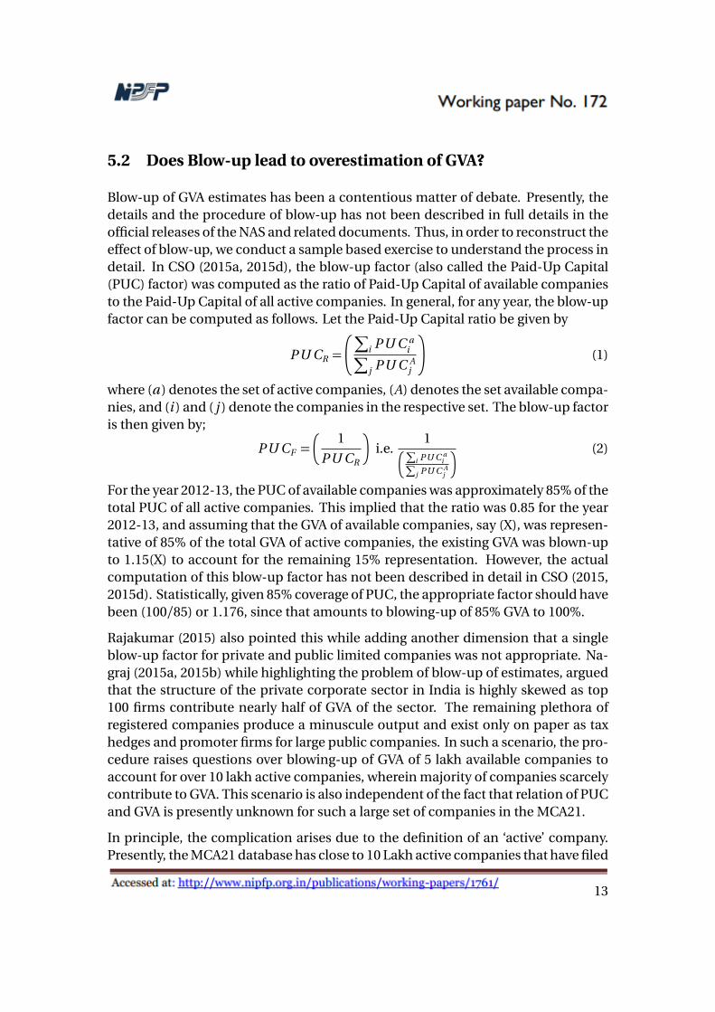
The question of Paid-Up Capital based blow-up of GVA leading to an overestimationis an important one. We construct an alternate methodology of blow-up by usingrepresentative industry growth rates of GVA to scale-up the previous GVA estimatesin case of unavailable companies. The purpose of the alternate method is to high-light the use of representative indicators for the sector, and also to arrive reasonablyclose to the actual estimates in case of data unavailability. We argue that this offersa possible solution to avoid using the Paid-up Capital factor.

Another crucial question to answer is whether manufacturing companies are be-ing correctly identified? The MCA21 dataset poses problems of identification of theeconomic activities of companies as it is based on the NIC codes contained in theCompany Identification Code (CIN). While CSO (2015b) highlights such a problem,they do not provide a systematic method of identification of companies. We usedata from CMIE Prowess to analyze this problem and also the extent of distortionin GVA due to misclassification of companies. To begin with, we first present thebasic sources and methods used in the new series and elaborate the process of GVAcomputation, as understood from CSO (2015a, 2015b and 2015d).

4 What is the process of GVA estimation?

The methodology adopted in the 2011-12 series is similar to the tradition RBI method,but differs in terms of computation. The RBI computed GVA based on its samplestudy of company finances and the estimates were blown-up on the basis of Paid-Up Capital of companies. In the case of estimating GVA using the MCA21 database,the CSO uses an active set of companies, which is defined as; ‘companies havingfiled their financials, at least once in the past three years’. Within this active set,the GVA for a particular year is estimated using the data of companies that is avail-able till a cut–off date of extraction (Dec. 1 of the previous year), while data for theremaining active companies is treated as unavailable. Thus, the GVA is estimatedusing the available data and is blown-up to account for the remaining active but un-available companies. In terms of sources and methods, Table 1 compares the basicchanges in the 2004-05 and 2011-12 series.

Table 1: Sources and methods in the manufacturing sectorBase Year 2004-05 2011-12Entity Establishment EnterpriseData source IIP + RBI + ASI IIP +MCA + ASIGVA computation Production approach Production approachOutput Sales Sales +Other incomeCompiled from CSO(2015b)

7

As part of a definitional change, GVA in the new series is estimated at the enterpriselevel. Previously, the establishment was limited to a factory registered under theFactories Act, that did not take into account the value addition at the head officeor related ancillary activities of the company. The estimation process continuesto be based on the production side identity of value addition, but uses the MCA21database instead of the RBI sample studies.

The changes in definition and data source have also led to changes in measures ofoutput, costs and intermediate consumption. In particular, the measures of out-put uses several disaggregated items of revenue in addition to industrial sales. Wedeal with these issues in detail in the following section. To re-create the process ofestimation, first the relevant details of the dataset and fields needs mention.

4.1 XBRL taxonomy

In the MCA21 database, the eXtensible Business Reporting Language (XBRL) for-mat has been made in concordance with the System of National Accounts (SNA)2008 description of items in the balance sheet and Profit and Loss account of com-panies. Presently, the XBRL has over 3400 fields wherein companies are requiredto furnish disaggregated information on various revenue, cost and balance sheetitems. These fields are utilized to construct the basic sequence of accounts, i.e. theproduction, generation of income, capital and distribution of income accounts asper the definitions of SNA. Similarly, for estimation of gross value addition, fieldsof the XBRL form are identified to estimate value of output and intermediate con-sumption (see the Goldar Committee’s Final report on the Private Corporate sectorincluding PPPs, CSO (2015b)). A complete description of the XBRL fields for thispurpose is given in Appendix A. In addition to identifying the fields, CSO (2015b)also prescribed the formula for computation of GVA using the production account.The items and formula are described in Appendix A.

4.2 Computation

To recreate the process of estimation, a company’s actual XBRL filing was obtainedfrom the MCA21 database to identify the fields for computation. Of the 3400 plusfields in the XBRL form, about 65 fields were used in the GVA formula. Using theproduction side formula prescribed in CSO (2015b), the GVA of the sample firm wascomputed as a benchmark estimate. The XBRL fields were then mapped to fieldsof financial data in CMIE Prowess and an alternate estimate was computed for thesample firm. A list of mapped fields is presented in Appendix B. The exercise was

8

then extended to all available firms in the manufacturing sector in CMIE Prowess.In order to maintain comparability of estimates with the CSO’s figures, a set of firmswas made that fulfilled the XBRL filing criteria in MCA21, namely; (i) company hav-ing paid-up capital greater than INR 5 crores or (ii) a turnover greater than INR 100crores or (iii) is a listed company. Table 2 presents the number and GVA of compa-nies using Prowess and compares it with the CSO’s estimate of companies that filein the XBRL format in the MCA21.

Table 2: Number of companies and GVA of manufacturing sectorusing CMIE Prowess (Current prices, Rs. Crore)

Year XBRL Co. GVA XBRL Co. GVA Manuf. Co. GVAin Prowess (Prowess) in MCA21 MCA21 in Prowess Manf. Co

1 2 3 4 5 6 72011-12 3017 684229.2 - 841623 4900 767311.72012-13 3010 744291.1 12682 943153 4154 819228.52013-14 2684 800106.6 - - 3674 8721782014-15 1915 772886.2 - - 2522 861641.6GVA computation is based on the formula in CSO (2015b), XBRL Co. and Manuf. Co.denote number of companies

We also use the pre-defined set of ‘manufacturing’ companies in Prowess to com-pute the GVA estimate. The difference between the XBRL criteria and the pre-definedProwess set is that the companies in the XBRL set are first identified using the 2 digitNIC 2008 codes for the manufacturing sector and subsequently the qualifying cri-teria is applied. Thus, using the Corporate Identification Number (CIN) code ofthe company, the 2 digit range of 10 - 33 was first applied to companies and sub-sequently, the XBRL qualifying criteria was used. In the case of Prowess, compa-nies are classified as ‘manufacturing’ based on their primary economic activity andproduct schedules.

Presently, in CSO (2015b) the disaggregated figures of GVA by industry groups andfiling criteria are available only for two years. The GVA figures for the manufacturingsector companies that file in XBRL are presented in columns 4 and 5. Comparingthese figures with our set from Prowess, it substantiates one of the arguments thata fraction of top (and large) companies contribute substantially to GVA. To developon this argument, we need a detailed scrutiny of the fields that are used for compu-tation of value addition and the size distribution of companies. To avoid problemsof classification of companies based on CIN codes, we use the manufacturing setof companies as defined in Prowess for the purpose of estimation. The problems ofidentifying and classifying a manufacturing company is dealt separately in Section7. The aggregate GVA of manufacturing companies that are comparable to compa-

9

nies filing in XBRL is given in column 7 for the year 2011-12. The computation ofthis aggregate is based on the mapping of fields with the XBRL form given in Ap-pendix A. Table 3 shows the disaggregation into three basic components, namelyoutput, taxes and subsidies and intermediate consumption.

Table 3: Components of GVA for manufacturing companies usingCMIE Prowess (Current prices, Rs. Crore)

S. No. Item 2011-12Output Revenue Sale of Product 3455812.45

Revenue from sale of services 10084.43Miscellaneous other operating revenue 301623.73Revenue from other financial services 59459.09Other miscellaneous non operating income 5956.07

A Value of output 3832935.77B Less: Change in Stock 38631.36

Taxes Indirect taxes 233717.26and Export incentives including duty draw back, etc. 7994.98

Subsidies Fiscal benefits (oil companies) 86761.59Sales tax and VAT benefits 368.86Other fiscal benefits and subsidies 43909.72

C Net Indirect taxes 94682.11Intermediate Raw materials stores spares 2099607.27Consumption Purchase of finished goods 620023.56

Royalties technical know how fees, etc. 11792.28Rent and lease rent 9212.21Repairs and maintenance 28216.21Insurance premium paid 3830.38Selling distribution expenses 144010.74Communications, IT expenses 1514.32Provision for Wealth tax 7.53Research and development expenses 14096.06

D Intermediate consumption 2932310.56A − B − C −D Gross Value Added 767311.74

Number of companies 4900

The major heads are further disaggregated into revenue and cost items, the detailsof which are given in Appendix 3. Using the production side identity, the GVA iscomputed as total value of output (market+own use) minus taxes and intermediateconsumption, where the task is to identify items that constitute value of output,taxes and intermediate consumption.

10

In mapping the XBRL and Prowess fields we highlight the possibility of incorrectlyidentifying a field as the definitions of items in both these datasets are not identi-cal. In the case of XBRL, the actual fields do not contain a definition and the detailsof the items can only be inferred from the labels attached to it. In some cases, ref-erences have been made to Schedule-III and the revised Schedule-IV of the Com-panies Act, 2013 for identifying components of the fields. However, for a majorityof items, the details in the schedules are insufficient to decide on inclusion or ex-clusion of an item or on the treatment of an amount given in subfields. In the caseof CMIE Prowess, items have been classified using definitions based on normaliza-tion to bring in homogeneity across companies as each one uses a non-standardnomenclature of financial items.

5 Issues in estimation

Based on the disaggregated fields used in the estimation, we highlight some issuesthat can have a considerable impact on the estimates. The first is of identificationof fields for measuring value of output at the firm level.

5.1 What are the measures of output and costs?

The GVA formula uses several disaggregated components of revenue that includesrevenues from products, services, operating revenues, revenue from financial ser-vices, rental income, incomes from brokerage & commission and other non-operatingincomes. The aggregate of the revenues is similar to the definition of total incomeof the company, which takes into account incomes from all business activities. Onthe cost side, the formula takes into account expenses related to production activ-ities, indirect taxes and other items such as rent, insurance, repairs and selling anddistribution expenses. For a comparison, we compute first GVA by taking industrialsales as a measure of output of the manufacturing activity and later include othersources of revenue as given in CSO (2015b). Table 4 compares the difference in GVAdue to addition of revenues from sources other than manufacturing.

11

Table 4: Values of GVA based on Industrial sales andother revenues as measure of output

Period Based on Gr. Rate Based on Gr. Rate Diff.Sales (%) Dis. Rev. (%)

1 2 3 4 5 62011-12 701896.6 - 767311.74 - 65415.12012-13 742237.2 5.74 819228.5 6.76 76991.32013-14 780371.1 5.13 872178.0 6.46 91806.9

In column 6 we show the difference in levels of GVA due to the addition of revenuefrom other sources. The addition to such revenues shows a considerable increasein GVA which possibly explain part of the large revisions in levels of 2011-12 for themanufacturing sector. The level change also corresponds to a 1% increase in growthrate of the sector.

Based on these revenue and cost items, one can identify sources of potential over-estimation of GVA. On the revenue side, the addition of non-operating revenues,financial services etc. constitutes a substantial part of revenue for large and di-versified firms. The representative indicator for the revenues generated solely outof manufacturing activities is industrial sales. Conventionally, subtracting the costitems (related to production) from sales provides a measure of value addition en-tirely from manufacturing activities. However, with large and diversified activities,identifying representative costs from financial data and aggregate data fields couldpose challenges, thereby leading to imprecise estimates. A close scrutiny of theXBRL fields shows omission of several important cost components, such as; Power &Fuel, advertisement and marketing related expenses. These are sizable componentsand their omission can significantly underestimate costs, thereby overestimatingGVA. It has also been pointed out in CSO’s reports that such post-manufacturingor ancillary activities are being captured as part of the new ‘enterprise’ approach.However, given the composition of business activities and diversification under oneroof, the value addition cannot be taken to be arising solely out of manufacturingactivities.

It is also important to note that since the GVA is computed using the productionside identity, a company for any given year may register a negative value addition.This is possible on account of large values of intermediate costs that can lead tolosses. While aggregating across companies, negative GVA contributions do not ap-pear prominently, but the extent of negative GVA contributions is certainly an issuein case of blow-up of estimates. Presently, in the absence of actual data of an activecompany, the existing GVA is blown-up based on the Paid-up Capital factor, while inpractice, the possibility of the company registering a negative GVA cannot be ruledout. We highlight such possibilities in the following section.

12

5.2 Does Blow-up lead to overestimation of GVA?

Blow-up of GVA estimates has been a contentious matter of debate. Presently, thedetails and the procedure of blow-up has not been described in full details in theofficial releases of the NAS and related documents. Thus, in order to reconstruct theeffect of blow-up, we conduct a sample based exercise to understand the process indetail. In CSO (2015a, 2015d), the blow-up factor (also called the Paid-Up Capital(PUC) factor) was computed as the ratio of Paid-Up Capital of available companiesto the Paid-Up Capital of all active companies. In general, for any year, the blow-upfactor can be computed as follows. Let the Paid-Up Capital ratio be given by

PU CR =

�∑

i PU C ai

∑

j PU C Aj

�

(1)

where (a ) denotes the set of active companies, (A) denotes the set available compa-nies, and (i ) and ( j ) denote the companies in the respective set. The blow-up factoris then given by;

PU CF =�

1

PU CR

�

i.e.1

�∑

i PU C ai

∑

j PU C Aj

� (2)

For the year 2012-13, the PUC of available companies was approximately 85% of thetotal PUC of all active companies. This implied that the ratio was 0.85 for the year2012-13, and assuming that the GVA of available companies, say (X), was represen-tative of 85% of the total GVA of active companies, the existing GVA was blown-upto 1.15(X) to account for the remaining 15% representation. However, the actualcomputation of this blow-up factor has not been described in detail in CSO (2015,2015d). Statistically, given 85% coverage of PUC, the appropriate factor should havebeen (100/85) or 1.176, since that amounts to blowing-up of 85% GVA to 100%.

Rajakumar (2015) also pointed this while adding another dimension that a singleblow-up factor for private and public limited companies was not appropriate. Na-graj (2015a, 2015b) while highlighting the problem of blow-up of estimates, arguedthat the structure of the private corporate sector in India is highly skewed as top100 firms contribute nearly half of GVA of the sector. The remaining plethora ofregistered companies produce a minuscule output and exist only on paper as taxhedges and promoter firms for large public companies. In such a scenario, the pro-cedure raises questions over blowing-up of GVA of 5 lakh available companies toaccount for over 10 lakh active companies, wherein majority of companies scarcelycontribute to GVA. This scenario is also independent of the fact that relation of PUCand GVA is presently unknown for such a large set of companies in the MCA21.

In principle, the complication arises due to the definition of an ‘active’ company.Presently, the MCA21 database has close to 10 Lakh active companies that have filed

13

their financial statements alteast once in the past 3 financial years. Thus, given thevariation in annual filing, the sample of available companies is also likely to differon a yearly basis. In view of such a variation, the blow-up factor would vary as itaccounts for the non-reporting companies. Using our existing sample of companiesthat qualifies the XBRL filing criteria, the effect of variation in the blow-up factor canbe seen as follows.

Table 5: Blow-up of GVA estimates using Paid-Up Capital factor, (Rs. Crores)S.No. CA Ca Sample % Pa PA PUC factor G V Aa Blown up Diff % Error

of Ca

�

1PaPA

�

(Rs. Cr.) GVA (6*7) of sample 1

1 2 3 4 5 6 7 8 9 101 3479 3479 100 137817 137817 1.000 757865 757865 0 0.002 3479 3306 95 130677 137817 1.050 707834 746510 −11354 −1.503 3479 3132 90 123905 137817 1.110 686168 763210 5345 0.714 3479 2958 85 119500 137817 1.150 656858 757541 −324 −0.045 3479 2784 80 100094 137817 1.380 593849 817653 59788 7.896 3479 2610 75 101511 137817 1.360 552675 750339 −7526 −0.99

Avg. 1.21SD 3.82

In Table 5, CA and Ca denote number of active and available companies, Sample %denotes the percentage of companies taken from the available set of 3479, Pa andPA denote Paid up capital of available and active companies, G V Aa denotes theGross Value Added of available companies, Diff denotes the difference of actual GVAof the 100% sample and blown up GVA of available companies, U Ca is the actualvalue of GVA of the unavailable or remaining companies that were not a part of thesample, and % error denotes the difference between the blown up and actual GVAas a percentage of the actual GVA (of sample 1).

The first sample is taken as 100 % in our case as data for the financial year (2011-12)is available only for 3479 XBRL qualifying companies. We then draw random sam-ples of companies from this set (3479) with different levels of coverage ranging from95% to 75%. These random samples represent the number of available companiesas shown in column 2, with the corresponding active set of companies given in col-umn 1. Columns 4 and 5 show the total Paid up Capital of each sample of compa-nies. In column 6, we compute the blow-up factor using equation (2) as describedearlier. Column 7 shows the GVA of available companies and column 8 shows theblown-up GVA by multiplying the factor to account for the unavailable companies.In column 9, we show the difference between the actual GVA of the 100% sampleand the blown-up GVA. A percentage error of the difference as compared to the ac-tual GVA is calculated for each sample in column 10.

The estimation procedure revels several shortcomings of this method. First, theblow-up factor is sensitive to Paid-up Capital coverage and can show a considerableincrease as the number of non-reporting companies increase. Second, the variation

14

in blown-up values is unpredictable as there is no systematic trend for different val-ues of the PUC factor. This leads to an unknown degree of error as the additiondue to blow-up can be significantly large as compared to the actual contribution ofunavailable companies. From the last column in Table 5, it is evident that, on av-erage, the error is positive and with large samples, this value can be of a significantproportion in terms of levels.

In the present case, statistically, our samples have only one realization. To get aclearer understanding of the blow-up effect, we can reconstruct the blow-up methodfor a particular sample. Analytically, a given level of sample coverage can be ob-tained from several random draws of companies from the active set. We experi-ment with two such cases. We fix the coverage to 80 and 85% and randomly draw100 samples in each case. Since our variable of interest is the Paid-Up Capital factor,we compute and plot the density based on these 100 samples. Figure 1 shows thedensity plot of PUC factor for two sample coverages.

Figure 1 : Density plot for Paid-Up Capital factorPUC factor distrubution computed for 80% and 85% sample coverages based on 100 random sam-

ples

1.1 1.2 1.3 1.4 1.5

01

23

45

6

N = 100 Bandwidth = 0.01872

Den

sity

PUC factor for 80% samplePUC factor for 85% sample

The distribution of PUC factor for a given sample coverage shows large variationsand with higher values it can lead to a considerable overestimation of GVA. The con-ceptual limitation of this method is that it uses the ratio of PUC to scale up existingGVA. The method is based on the assumption that PUC and GVA have a one-to-onecorrespondence and that the Paid up Capital of a company can be used to estimate

15

its GVA contribution. This is at best a weak assumption, as one cannot draw suffi-cient inference about a company’s manufacturing activities by looking at its Paid-upCapital value.

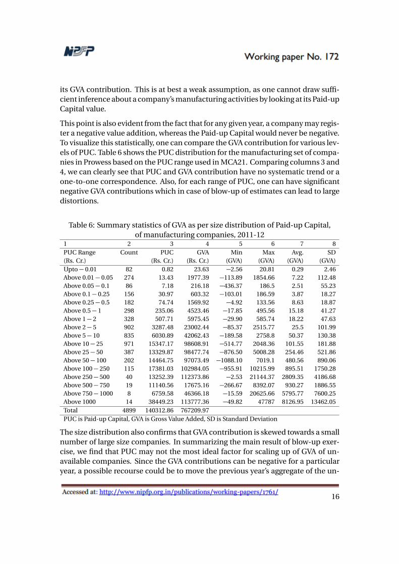
This point is also evident from the fact that for any given year, a company may regis-ter a negative value addition, whereas the Paid-up Capital would never be negative.To visualize this statistically, one can compare the GVA contribution for various lev-els of PUC. Table 6 shows the PUC distribution for the manufacturing set of compa-nies in Prowess based on the PUC range used in MCA21. Comparing columns 3 and4, we can clearly see that PUC and GVA contribution have no systematic trend or aone-to-one correspondence. Also, for each range of PUC, one can have significantnegative GVA contributions which in case of blow-up of estimates can lead to largedistortions.

Table 6: Summary statistics of GVA as per size distribution of Paid-up Capital,of manufacturing companies, 2011-12

1 2 3 4 5 6 7 8PUC Range Count PUC GVA Min Max Avg. SD(Rs. Cr.) (Rs. Cr.) (Rs. Cr.) (GVA) (GVA) (GVA) (GVA)Upto − 0.01 82 0.82 23.63 −2.56 20.81 0.29 2.46Above 0.01 − 0.05 274 13.43 1977.39 −113.89 1854.66 7.22 112.48Above 0.05 − 0.1 86 7.18 216.18 −436.37 186.5 2.51 55.23Above 0.1 − 0.25 156 30.97 603.32 −103.01 186.59 3.87 18.27Above 0.25 − 0.5 182 74.74 1569.92 −4.92 133.56 8.63 18.87Above 0.5 − 1 298 235.06 4523.46 −17.85 495.56 15.18 41.27Above 1 − 2 328 507.71 5975.45 −29.90 585.74 18.22 47.63Above 2 − 5 902 3287.48 23002.44 −85.37 2515.77 25.5 101.99Above 5 − 10 835 6030.89 42062.43 −189.58 2758.8 50.37 130.38Above 10 − 25 971 15347.17 98608.91 −514.77 2048.36 101.55 181.88Above 25 − 50 387 13329.87 98477.74 −876.50 5008.28 254.46 521.86Above 50 − 100 202 14464.75 97073.49 −1088.10 7019.1 480.56 890.06Above 100 − 250 115 17381.03 102984.05 −955.91 10215.99 895.51 1750.28Above 250 − 500 40 13252.39 112373.86 −2.53 21144.37 2809.35 4186.68Above 500 − 750 19 11140.56 17675.16 −266.67 8392.07 930.27 1886.55Above 750 − 1000 8 6759.58 46366.18 −15.59 20625.66 5795.77 7600.25Above 1000 14 38449.23 113777.36 −49.82 47787 8126.95 13462.05Total 4899 140312.86 767209.97PUC is Paid-up Capital, GVA is Gross Value Added, SD is Standard Deviation

The size distribution also confirms that GVA contribution is skewed towards a smallnumber of large size companies. In summarizing the main result of blow-up exer-cise, we find that PUC may not the most ideal factor for scaling up of GVA of un-available companies. Since the GVA contributions can be negative for a particularyear, a possible recourse could be to move the previous year’s aggregate of the un-

16

available companies by the representative industry growth rate. Such a method canavoid the use of Paid up Capital factor as in absence of any other information, therepresentative industry growth rate can serve as a sufficient indicator for capturingthe business environment faced by firms in that industry. We explore this methodas an alternative in the following section.

In the annual filing by companies, the process of identifying the correct set of finan-cial data is also a matter of concern. It is well known that companies also file theirfinancial accounts for periods less than 12 months and 18 month or more. Withinthe active set, such filing can complicate the identification of data for a particularyear for computation. For instance, given the current cutoff date of data extractionfrom the MCA21, the process does not elaborate on the treatment of financial state-ments filed for less than 12 months or for a 18 month period. This creates a problemfor a particular year as the data for such companies has to be either apportioned for12 months or considered for the following year. At present, no method or criteriahas been specified to deal with this issue.

The magnitude of this problem or the distortion due to such filing is presently un-known, but nevertheless, it requires a systematic process to address the issue. Oneof the gains of moving to MCA21 has been to achieve a wider coverage of companiesin the overall private corporate sector. However, as the year-on-year filing is likelyto vary, a feasible process would be take data of companies on a frame or surveybasis such that the annual variation in data availability can be minimized.

6 An alternate method of blow-up

As an alternative to using the Paid-Up Capital factor for blow-up of available GVA,we explore the possibility of using representative industry growth rates to move for-ward the previous year’s GVA of unavailable companies. Using sectoral growth ratesto move benchmark estimates for future years is an existing and acceptable methodto account for data unavailability. Such methods are already in place for movingseveral lead indicators in the national accounts. Rao (2015) has made similar ob-servations regarding alternate methods to blow-up of GVA. Similarly, in the case ofmanufacturing sector, industry wise growth rates are a reflection of the businessenvironment of a given sector and should capture, on average, the performance ofcompanies in that sector. This method gives an advantage over the PUC factor asit can capture the trends and volatility of the economic conditions faced by busi-nesses. Thus, issues of economic downturns, negative GVAs or non-filing by com-panies can be addressed without having to resort to a blow-up factor that does nottake into account such aspects.

17

To elaborate the process, we first construct the industry wide growth rates of GVAusing our sample of companies in Prowess. Since Prowess reports industry groupsand product codes, we are able to separate companies into various industry groups.For a particular year, we take a moving average of the past three years of the GVA lev-els to smoothen out the year-on-year fluctuations. We then take an annual growthrate of these levels and consider that as a representative indicator for the sector. Ta-ble 7 tabulates the 3 year moving average of the levels and the corresponding growthrates of the sectors based on all available companies.

Table 7: 3 year moving average of levels of avail. GVA by industry(Rs. Crore) and corresponding growth rates

GVA GVA GVA GVA Gr. % Gr. % Gr. %Industry 08-09 09-10 10-11 11-12 09-10 10-11 11-12Agri. products 4855.61 5870.29 6792.27 7635.38 20.897 15.706 12.413Animal products 932.99 968.60 1010.92 844.28 3.816 4.369 −16.484Base Metals 107610.61 119730.23 122965.26 136082.70 11.262 2.702 10.668Chemicals 67554.98 78468.96 91532.86 101168.74 16.156 16.648 10.527Diversified 19726.20 22928.43 23700.16 27165.84 16.233 3.366 14.623Fats, oils, etc. 3219.08 3838.01 4314.08 4611.31 19.227 12.404 6.890Food, beverages, etc. 23860.44 25902.42 29082.64 30634.25 8.558 12.278 5.335Leather products 1226.62 1376.83 1471.15 1574.48 12.246 6.850 7.024Machinery 57045.96 65782.43 73719.64 81740.56 15.315 12.066 10.880Mineral products 72893.64 74350.85 75475.78 75752.66 1.999 1.513 0.367Misc. Manuf. 945.16 898.77 925.02 947.98 -4.908 2.920 2.482Non metallic 40588.68 48176.47 53833.85 62892.67 18.694 11.743 16.827Others 82.48 80.28 72.66 207.22 -2.663 -9.492 185.196Plastics & rubbers 15442.97 17761.09 19472.96 21477.10 15.011 9.638 10.292Pulp & paper 8368.84 10554.44 12931.83 14768.29 26.116 22.525 14.201Textiles 33630.22 38584.72 42048.12 43087.00 14.732 8.976 2.471Transport equipment 32691.05 37594.89 44953.76 53625.98 15.001 19.574 19.291Wood products 536.04 725.24 833.78 925.96 35.296 14.965 11.056Total 491211.57 553592.96 605136.73 665142.40 12.699 9.311 9.916

We use data of the 80% sample as in the case of blow-up (see sample 5 in Table 3)as an illustration and identify the sector of the missing companies. Since, by def-inition, the unavailable company is a part of the active set, we would expect thecompany to have filed its financials at least once in the past three years. For theunavailable companies, instead of using the Paid-up Capital, we search for the lastyear in which data is available for all such companies. For each year, we then clas-sify all missing companies (695) into their respective industry groups. This givesus a year wise set of companies in each industry group wherein the last estimateof GVA is available, as shown in column 1. Upon identifying past data, we pick therelevant growth rates computed in Table 7 for the corresponding year for each in-dustry group. In this particular sample, data of all companies was available within

18

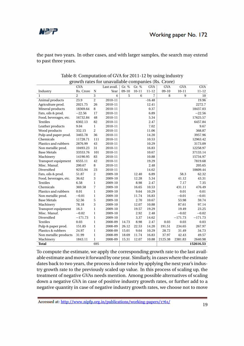
the past two years. In other cases, and with larger samples, the search may extendto past three years.

Table 8: Computation of GVA for 2011-12 by using industrygrowth rates for unavailable companies (Rs. Crore)

GVA Last avail. Gr. % Gr. % GVA GVA GVA GVAIndustry Rs. Crore N Year 09-10 10-11 11-12 09-10 10-11 11-121 2 3 4 5 6 7 8 9 10Animal products 23.9 2 2010-11 -16.48 19.96Agriculture prod. 2021.75 26 2010-11 12.41 2272.7Mineral products 18369.64 8 2010-11 0.37 18437.03Fats, oils & prod. −22.56 17 2010-11 6.89 −22.56Food, beverages, etc. 16732.84 48 2010-11 5.34 17625.57Textiles 6302.13 82 2010-11 2.47 6457.84Leather products 9.04 1 2010-11 7.02 9.67Wood products 332.15 2 2010-11 11.06 368.87Pulp and paper prod. 3465.78 36 2010-11 14.20 3957.96Chemicals 11728.71 111 2010-11 10.53 12963.42Plastics and rubbers 2876.99 43 2010-11 10.29 3173.09Non metallic prod. 10493.23 31 2010-11 16.83 12258.97Base Metals 33553.76 101 2010-11 10.67 37133.14Machinery 14190.95 83 2010-11 10.88 15734.97Transport equipment 6555.11 42 2010-11 19.29 7819.68Misc. Manuf. 200.67 8 2010-11 2.48 205.65Diversified 9255.94 23 2010-11 14.62 10609.44Fats, oils & prod. 51.87 2 2009-10 12.40 6.89 58.3 62.32Food, beverages, etc. 36.62 3 2009-10 12.28 5.34 41.12 43.31Textiles 6.58 1 2009-10 8.98 2.47 7.17 7.35Chemicals 369.58 7 2009-10 16.65 10.53 431.11 476.49Plastics and rubbers 0.01 1 2009-10 9.64 10.29 0.01 0.01Non metallic prod. −0.01 1 2009-10 11.74 16.83 −0.01 −0.01Base Metals 52.56 5 2009-10 2.70 10.67 53.98 59.74Machinery 78.18 3 2009-10 12.07 10.88 87.61 97.14Transport equipment 16.3 1 2009-10 19.57 19.29 19.49 23.25Misc. Manuf. −0.02 1 2009-10 2.92 2.48 −0.02 −0.02Diversified −171.73 1 2009-10 3.37 14.62 −171.73 −171.73Textiles 0.03 1 2008-09 14.73 8.98 2.47 0.03 0.03 0.03Pulp & paper prod. 151.85 1 2008-09 26.12 22.53 14.20 191.51 234.65 267.97Plastics & rubbers 24.97 1 2008-09 15.01 9.64 10.29 28.72 31.49 34.73Non metallic products 31.99 1 2008-09 18.69 11.74 16.83 37.97 42.43 49.57Machinery 1843.11 1 2008-09 15.31 12.07 10.88 2125.38 2381.83 2640.98Total 695 152616.53

To compute the estimate, we apply the corresponding growth rate to the last avail-able estimate and move it forward by one year. Similarly, in cases where the estimatedates back to two years, the process is done twice by applying the next year’s indus-try growth rate to the previously scaled up value. In this process of scaling up, thetreatment of negative GVAs needs mention. Among possible alternatives of scalingdown a negative GVA in case of positive industry growth rates, or further add to anegative quantity in case of negative industry growth rates, we choose not to move

19

the negative value and use the same value for the next year. This is based on thepremise that one cannot make apriori judgments about a firm’s loss making situa-tions. In the case where the representative industry growth rates are positive, a lossmaking firm in the industry can only be assumed to reduce its losses or may turnprofitable over a period of time. However, in absence of any firm level information,moving the GVA in either direction could be misleading and will cause an unknowndegree of error. Although in this method the effect of scaling the negative value onthe aggregate GVA is negligible, not moving it ensures that it will not contribute pos-itively as in the case of blow-up using PUC factor. Lastly, we move all estimates tillthe current year (2011-12) and aggregate it to represent the scaled up estimate toaccount for the missing companies. Repeating this process for the same samplesas in the case of blow-up, we get comparable estimates from both methods. Table9 presents the figures for all samples for this method and compares then with thePUC factor based method.

Table 9: Estimate of scale up using industry wise growth ratesSample CA Ca Sample % G V Aa Blown up GVA of GVA scaled GVA scaled % Error % Error

of Ca GVA U Ca by PUC factor by Ind. Gr. PUC factor Ind. Gr.1 2 3 4 5 6 7 8 9 10

1 3479 3479 100 757865 757865 0 0 0 - -2 3479 3306 95 707834 746510 50031 38676 41518 −1.50 −1.123 3479 3132 90 686168 763210 71697 77042 60807 0.71 −1.434 3479 2958 85 656858 757541 101007 100682 109894 −0.04 1.175 3479 2784 80 593849 817653 164015 223804 152616 7.89 −1.506 3479 2610 75 552675 750339 205189 197663 199134 −0.99 −0.80

Avg. 1.21 -0.74SD 3.826 1.101

In Table 9, (CA) and (Ca ) denote number of active and available companies, Sample% denotes the percentage of companies taken from the available set of 3479, G V Aa

denotes the Gross Value Added of available companies, Diff denotes the differenceof actual and blown up GVA of available companies, U Ca is the actual value of GVAof the unavailable or remaining companies that were not a part of the sample, andInd. Gr. denotes the GVA scaled by applying industry growth rates to previous year’sGVA for missing companies. % error denotes the difference between the blown upand actual GVA as a percentage of the actual GVA (of sample 1) by both methods.This comparison is essential as it provides a direction and magnitude of the errorin estimation. Column 7 gives the addition due blow-up based on the PUC factor,while column 8 gives the figures based on industry growth rates. Comparing thefigures with the actual figure of the unavailable companies (column 6), the extentof blow-up based on the PUC factor can be clearly observed.

The figures based on industry growth rates are considerably close to the actual val-ues, thereby substantiating that industry growth rates are reflective of the perfor-

20

mance and value addition by companies in the sector. Comparing the percent-age errors due to both methods, the second method leads to an underestimationof value addition. On average, the error is negative (−0.74) with a lesser degree ofvariability across samples. In constructing the alternate method, the focus has beento use an indicator that is reflective of the business environment faced by the com-pany in an industry, and to get an estimate that is closer to the actual contributionof the unavailable companies.

In practice, as in the case of CSO, the actual estimate of the unavailable companiesfor any given year is possibly unknown. In such a case, errors in estimation of lev-els will eventually translate into incorrect growth rates, thereby not reflecting thetrue picture of the sector. For instance, overestimation in a year would led to largerevisions of the data in the following year as the actual data becomes available. Sim-ilarly, underestimation in a year and overestimation in a following would magnifyand overstate the growth rates, where in fact, the true picture of the growth in re-spective industries may be unknown. Thus, in absence of data availability, choosinga method that is in part reflective of the business activities and provides estimateswith a lower degree of error could greatly enhance the reliability of the estimates.

7 Issues in identifying manufacturing companies

The second key question is that are manufacturing companies being correctly iden-tified? In the MCA21 database, the CSO relied on using CIN code to identify man-ufacturing companies. The decision to use CIN was made as the ITC-HS codes ofproducts were either unreported or unavailable in the XBRL forms (CSO, 2015d).However, in absence of the ITC-HS codes, using CIN code can potentially lead to amisclassification of companies in identifying their business activity. This is primar-ily due to the fact that CIN, which contains the NIC classification, does not undergoa change once it has been created for a company. Over time, a company may changethe nature of its business activity or diversify into any other sector. While doingso, the change of business activity is not reflected in the CIN code of the company.Thus, using CIN can be potentially misleading for identifying the nature of businessof a company since its top revenue generating activity might be different from theone mentioned in its CIN code.

Also, the NIC classification undergoes a change over time as it is part of a systemicprocess of updation of industrial classification. This adds to the complexity of iden-tification in two ways; first, changes in business activities of companies are inde-pendent of changes in NIC codes, and second, a particular NIC code may not re-flect the same business activity over time. While the problem in using CIN code

21

was briefly raised in CSO (2015d), no systematic recourse was mentioned. To high-light this problem, Prowess database was used to construct a list of companies thatwere registered with CIN in manufacturing but had their main revenue generatingproduct from a different economic activity. The list of companies is presented inTable 10.

Table 10: Business activity of companies with CIN registered in manufacturing(NIC 2008 2 digit classification code 10 - 33)

Industry activity (2 digit) Number Industry activity (2 digit) NumberTrade in other manufactured goods 362 Financial services including leasing 328Other asset financing services 279 Securities investment services 275Renting services 163 Services 128Software services 81 Commission agents services 76Trade in electrical machinery 76 Trade in manufactured products 63Trade in chemicals 59 Trade in minerals & energy sources 57Real estate infrastructure services 54 Trade in transport equipment 49Trade in drugs & medicines 48 Business services 43Trading in food products 43 Trade in agricultural crops 40Tech. Consultancy & Engg. serv. 31 Info. Tech Enabled Service/BPO 21Hotel & restaurant service 22 Other Consultancy 17Fund based financial services 19 Trade in non-electrical machinery 15Finance related allied activities 15 Shipping services 13Printing and related services 13 Research & development 10Storage & warehousing services 11

In the manufacturing sector, it is common to find that several companies operateas wholesale trading, financing, renting or as service providers in the name of man-ufacturing. A reverse problem could also exist, wherein companies registered inother economic activities may undertake manufacturing activities. Since the mis-classification may lead to a distortion in the overall estimate, we compute the mag-nitude by estimating the GVA for such companies.

Table 11: GVA of companies with registered economic activityother than manufacturing, 2011-2012 (Rs. Crores)

Year Cw m GVA Cw m Co m GVA Co m

2011-12 539 17630.00 1083 173689.11

Table 11 shows the estimates of two categories of companies. Cw m denotes thenumber of wrongly classified companies, i.e. with registered CIN code in manu-facturing but not having manufacturing as their primary activity, and Co m as thecompanies registered outside the manufacturing sector but having manufacturingas their primary activity. To visualize this in detail, we tabulate the break-up of GVAof such companies that may not get captured as part of manufacturing companiesbased on the NIC code contained in their company identification (CIN).

22

Table 12: Disaggregated GVA of companies with registered economic activityother than manufacturing, 2011-2012 (Rs. Crores)

Industry Count GVATransport equipment 142 43754.37Machinery 162 40778.74Base Metals 142 23438.58Chemicals 117 17131.28Food products, beverages & tobacco 65 10158.80Non metallic mineral products 71 9494.67Textiles 113 8378.18Plastics and rubbers 67 6548.16Mineral products 21 5412.47Agriculture products 69 4270.52Pulp and paper products 29 1532.36Leather products 13 868.17Fats & oils and derived products 19 835.02Misc. Manufactured Articles 46 768.02Wood products 5 227.96Animal products 2 91.81Total 1083 173689.11

The distortion in estimates due to misclassification can be substantial as indicatedby the values of GVA. The classification problem is of crucial importance since it isequally difficult to identify the business activity of a company through its financialstatements or registered economic activity. Instead, a more appropriate method isto scrutinize the product schedules to identify its primary activity and its top rev-enue generating product. The classification procedure requires a more careful andscientific approach to identify companies as it can distort the estimates significantlyand bring in computational problems for future years.

The estimates of the overall sector are obtained as a sum of value addition in the or-ganized and unorganized manufacturing sectors. The estimates of the unorganizedmanufacturing sector are computed from the data on Non-Corporate ASI and thefinal estimate of the sector is available with a lag of two years. Given the new methodof computation using the MCA21, one can take note of the differences with the ASImethod. First, the ASI approach continues to be based on the establishment ap-proach, wherein the enumeration unit is a factory registered under the FactoriesAct. Second, entities falling under the unorganized sector are less likely to have rev-enues from diversified business activities, thus making the enterprise and establish-ment concept similar. However, in terms of computation, the GVA formula used inthe ASI is more attuned to the concept of value addition as it clearly identifies thecontributing items to output and costs; see for instance, block J, D &, G for outputsand blocks F, H, & I in ASI (2011). Given the complexity of fields in the XBRL format,

23

in order to make the shift from establishment to enterprise approach, it would bemeaningful to first identify the fields similar to the establishment approach so as toclearly measure the outputs and inputs and further augment it to include fields thatcapture the value addition at the enterprise level. This distinction will also help inreconciling value addition in both organized and unorganized sectors, and in par-ticular, account for the changes in business activities over time.

8 Conclusion

The release of the NAS 2015 presented the new 2011-12 series of macro aggregatesafter a comprehensive revision of methodology and data sources in many sectors.The new 2011-12 series also attracted attention as it presented a macro picture that,in general, did not conform to expectations and assessments of various stakehold-ers. Within the overall GDP, the general discontent with the estimates of the man-ufacturing sector was driven by the fact that large upward revisions in growth ratesfrom 2011-12 were not reflective of the actual growth performance of the sector.Consequently, the official figures generated more questions than answers, and evenas various stakeholders continued to engage in decoding the mystery behind thelevels and growth rates, the debates and questions have not withered out.

On the questions of inconsistency and reliability of the estimates of the manufac-turing sector, the literature at many places has overlooked the finer details of newdefinitions and dataset used for GVA computation. We use the information avail-able in CSO (2015b) we recreate the estimation procedure to provide answers to twokey questions in the debate. First, does the Paid-Up Capital based blow-up methodlead to overestimation of GVA? and second, are manufacturing companies beingcorrectly identified in the MCA21 dataset.

We use a CMIE Prowess as comparable dataset to MCA21 to estimate the levels ofGVA for the manufacturing set of companies that file in the XBRL format in theMCA21. We also construct an alternate method of using representative industrygrowth rates to account for data of unavailable companies as a possible solution toavoid using the Paid-up capital factor. In a mapping of fields of the XBRL form andCMIE Prowess, we find that choice of revenue items to measure output can resultinto a considerable distortion in value of output at the firm level. Since the com-putation also includes revenues from several non-manufacturing activities, it canlead to overestimation of GVA as revenues from financial and other services cannotbe taken to reflect the value arising solely out of manufacturing activities. On thecost side, a close scrutiny of the XBRL fields show omission of few important costitems, such as; Power & Fuel expenses, advertisement and marketing related ex-

24

penses. These components are significant for manufacturing and diversified com-panies and their omission can significantly underestimate costs, thereby leading tooverestimation of GVA. While the new concept of estimating GVA is based on the en-terprise approach, the process of identifying outputs and costs remains ambiguousand unclear.

We conduct a sample based exercise to understand the blow-up procedure and findthat the blow-up factor is sensitive to Paid-up capital coverage and increases con-siderably with the variation in annual filing by companies. Since the GVA contri-bution for a firm can be negative for a particular year, the blow-up can lead to anoverestimation as scaling up always contributes positively, whereas the actual con-tribution of a company may be negative. The addition due to blow-up also remainsunpredictable, thereby leaving a scope for an error in estimation.

We propose an alternate method of scaling up by using representative industry growthrates of GVA to move forward the previous estimates of unavailable companies. Wefind that using the industry growth rate has an advantage over the PUC factor asit can capture the economic conditions faced by companies in different industries.The estimates moved forward using the growth rates closely resemble the actualcontribution of unavailable companies, thereby making the estimates more reflec-tive of the economic conditions of the sector. On average, the error in the PUC fac-tor based method is positive and may vary considerably, while it is negative in thegrowth rate based method. We argue that this procedure can reduce the problemof overestimation and at the same time bring more predictability and reliability tothe estimates.

We answer the second question by showing that misclassification of companies inthe MCA21 dataset can be a potential source of distortion of the GVA estimate. It iswell known that several companies operate as trading, financing or leasing compa-nies in the name of manufacturing. This complicates the process of identifying thenature of business activity or the top revenue generating product of the company.The identification problem requires a scientific and consistent solution, especiallywhen the present number is in excess of 10 lakh and new companies are added yearon year. Lastly, for the purpose for preparing the national accounts, it is imperativethat we get consistent and reliable data. However, in absence of data, one has toresort to alternative methods that can provide meaningful estimates. The focus inthis paper has been to consider one such alternative method.

Overall, the findings have highlighted that there are contentious issues in the pro-cess of estimation and identification of companies, before we make a judgment onthe sector’s growth figures. After the estimation process has been replicated, a closescrutiny of the components of GVA provide the much needed insights into the new

25

series. Qualitatively, the findings also change our view about the value additionoriginating from the manufacturing sector. While the new enterprise approach iswider in coverage and on lines of the SNA, the points of focus are essentially on theitems that make up for value of output and costs. Lastly, in the current scenario,there is limited availability of information on the MCA21 dataset and the actual es-timation procedure. A detailed documentation by the CSO on the procedure of es-timation is needed to bring more clarity and understanding of the estimates of thesector.

* * * * * * *

26

Appendix

A Mapping of XBRL fields with CMIE Prowess dataset

(See notes to variables in Section C for details and definitions)S.No. XBRL Fields: Production Account Prowess Fields

1 Market output =2 (8) RevenueFromSaleOfProducts Sales of Goods3 Add (9) RevenueFromSaleOfServices Inc. from Raw Mat. & after sales services4 Add (43) MiscellaneousOtherOperatingRevenues Inc. from scrap, Raw Mat., Job work, etc.5 Add (15) RevenueFromOtherFinancialServices Dividends, Interest income, Other fee based

services, hire-purchase, Bill discountingtreasury operations, gain of forex trans.

6 Add (47) RentalIncomeOnInvestmentProperty Rent Income7 Add (66) IncomeFromPipelineTransportation NA8 Add (60) IncomeOnBrokerageCommission Brokerage, service fee9 Add (63) OtherAllowancesDeductionOtherIncome Other non- operating income

10 Add (64) MiscellaneousOtherNonoperatingIncome Net Prior period & extra. ord. income11 Add (10) ExciseDuty Excise duty12 Add (11) ServiceTaxCollected Service tax13 Add (12) OtherDutiesTaxesCollected Other indirect taxes14 Minus (21) ChangesInInventories... Change in stock15 Minus (20) PurchasesOfStockInTrade Purchase of finished goods16 Minus (19) CostOfMaterialsConsumed (for trade) (for trade only)17 Output for own final use =18 Add (117) ExtractionCostPertainingToEAndPActivities NA19 Add (119) GeologicalAndGeophysical.. NA20 Add (121) ResearchAndDevelopment.. Included in item (93)21 Add (122) PipelineOperationAnd.. NA22 Add (123) OtherExpenditure NA23 (Taxes - subsidies) on products & imports =24 (10) ExciseDuty Excise duty25 Add (11) ServiceTaxCollected Service tax26 Add (12) OtherDutiesTaxesCollected Other Indirect taxes27 Minus (54) IncomeGovernmentGrantsSubsidies Subsidies28 Minus (55) IncomeExportIncentives Other Fiscal benefits29 Minus (61) IncomeOnSalesTaxBenefit Sales tax & VAT benefits30 Intermediate consumption =31 (19) CostOfMaterialsConsumed (for non-trade) Raw materials, stores & spares32 Add (28) ExpenditureOnProductionEandPactivities NA33 Minus (113) RoyaltyPertainingToEAndPActivities NA34 Minus (114) CessPertainingToEAndPActivities NA35 Minus (115) EducationCessPertainingToEAndPActivities NA36 Minus (116) NationalCalamityContingency.. NA37 Add (29) OtherExpenses [=38 (83) Rent + (84) RepairsToBuilding + (85) Rent & Lease rent39 RepairsToMachinery + (86) Insurance + (92) Repairs, Insurance premium paid40 RatesAndTaxesExcludingTaxesOnIncome + NA41 (93) ResearchDevelopmentExpenditure + (94) InformationTechnologyExpenses + R&D Expenditure42 (95) DonationsSubscriptions + (96) TransportationDistributionExpenses + Communication Exp.43 (97) CostRepairsMaintenanceOtherAssets + (98)CostInformationTechnology + Repair & Maintenance44 (99) CostInsurance + (100) CostOctroi + (101) CostTransportation + Selling & Dist. expenses45 (102) CostLeaseRentals + (103) CostRoyalty + (104) Included in Lease Rent46 ProvisionBadDoubtfulDebtsCreated + (105) Canceling47 ProvisionBadDoubtfulLoansAdvancesCreated + Canceling48 (106) AdjustmentsToCarryingAmountsOfInvestments + (107) NA49 NetProvisionsCharged + (108) DiscountIssueSharesDebenturesWrittenOff + Canceling50 (110) WriteOffAssetsLiabilities + (111) LossOnDisposalOfIntangibleAsset + Canceling51 (112) LossOnDisposalDiscard..] Canceling52 Minus (83) Rent Rent53 Minus (91) ProvisionWealthTax Prov. for Wealth Tax54 Minus (95) DonationsSubscriptions Canceling55 Minus (103) CostRoyalty Canceling56 Minus (104) ProvisionBadDoubtfulDebtsCreated Canceling57 Minus (105) ProvisionBadDoubtfulLoansAdvancesCreated Canceling58 Minus (107) NetProvisionsCharged Canceling59 Minus (108) DiscountIssueSharesDebenturesWrittenOff Canceling60 Minus (111) LossOnDisposalOfIntangibleAsset Canceling61 Minus (112) LossOnDisposalDiscardDemolishment.. Canceling62 Add (74) CommissionEmployees NA63 Add (82) OtherEmployeeRelatedExpenses NA64 Add (69) OtherBorrowingCosts NA

Source: CSO (2015b)

B Computation of GVA using XBRL fields

GVA formula based on Production approachP1 OutputP.11 Market Output including taxes

Sl. No. (8+9+43+15+47+66+60+63+64+10+11+12−21−20−19 (only for trade)P.12 Output for own final use: Sl. No. (117+119+121+122+123)P.13 Output for non-market use– NILD.21– D.31 Taxes and Subsidies: Sl. No.(10+11+12−54−55−61)P2 Intermediate Consumption (IC)

Sl. No.(19 (only for nontrade) + (28−113−114−115−116) + (29−83−91−95−103−104−105−107−108−111−112) +74+82+69)

B1 GVA: [P.11 + P.12 + P.13 − (D.21−D.31)]−P2Source: CSO (2015b)

Fields for computation of GVA using CMIE Prowess (Rs. Crore)Items / Sub-items Variable 2011-12 | Rs. Crore

1 Revenue from sale of products 3455812.51.1 Sales of goods 3455812.452 Revenue from sale of services 10084.43

2.1 Income from repairs, maintenance including after sales service 10084.433 Misc. other operating revenues 301623.73

3.1 Sale of scrap 9416.293.2 Sale of raw materials and stores 8673.863.3 Job work income 10947.363.4 Construction income 58320.793.5 Sale of electricity gas and water 26181.543.6 Other industrial sales 8998.013.7 Trading income 179085.884 Rental Income on investment and property 870.16

4.1 Rent income 870.165 Revenue from other Financial service 59459.09

5.1 Brokerage and financial service fees 31.365.2 Gain on securities transactions 10012.835.3 Gain relating to forex transactions 4597.55.4 Income from other treasury operations 17.095.5 Dividends 8398.715.6 Interest income 33383.295.7 Other fee based financial services 8.565.8 Bill discounting 0.235.9 Income from leasing, hire purchase and adjustment 3009.526 Miscellaneous other Non-operating Income 5085.91

6.1 Net Prior period and extra ordinary income 5085.91A Value of Output 3832935.87. Change in Stock 38631.36B Less: Change in stock 38631.368 Indirect taxes 233717.269 Less: Subsidies 139035.15

9.1 Export incentives including duty draw back etc 7994.989.2 Fiscal benefits to oil companies 86761.599.3 Sales tax and VAT benefits 368.869.4 Other fiscal benefits and subsidies 43909.72C Net Indirect taxes 94682.11

10.1 Raw materials stores and spares 2099607.2710.2 Purchase of finished goods 620023.5610.3 Royalties technical know how fees, etc. 11792.2810.4 Rent and lease rent 9212.2110.5 Repairs and maintenance 28216.2110.6 Insurance premium paid 3830.3810.7 Selling distribution expenses 144010.7410.8 Communications and IT services expenses 1514.3210.9 Provision for Wealth tax 7.5310.1 Research and development expenses 14096.06

D Intermediate consumption 2932310.6A−B−C−D Gross Value Added 767311.74

28

C Notes and Variable description

C.1 Notes

• Fields denoted as ‘NA’ were not available in CMIE Prowess database.

• Presently, a detailed definition of fields of XBRL is not available. The mean-ing of a field can only be inferred from the heading and labels attached to itin the XBRL taxonomy available from the Ministry of Corporate Affairs (MCA)website. Some details about the fields can be obtained from Schedule - III ,General instructions for preparation of Balance Sheet and statement of Profitand Loss of a company, Companies Act, 2013 and Guidance Note on the re-vised Schedule - VI, Companies Act, 1956.

C.2 Variable description

1. Sales of Goods: Income generated by companies from the sale of goods man-ufactured, or by sale of minerals extracted.

2. Sale of scrap: Income generated through the sale of scrap and waste and isdefined as incidental residue from certain types of manufacture, usually ofsmall amount and low value, recoverable without further processing

3. Income from repairs, maintenance, including after sales service income:Income earned by providing repairs and maintenance services. Repairs referto restoring an asset to sound condition. Maintenance, on the other hand,refers to upkeep of property or equipment.

4. Job work income: Income generated by a company when it undertakes con-tractual manufacturing or processing of a product as per client’s specifica-tions.

5. Sale of raw materials and stores: Includes the sale of raw materials as well assale of stores.

6. Construction income: Income earned by companies from construction andconstruction related activities.

7. Sale of electricity, gas and water: Income from electricity and gas relatedactivities can be in the form of sale of electricity, meter hire charges, wheel-ing charges, other electricity service charges, sale of piped natural gas, sale of

29

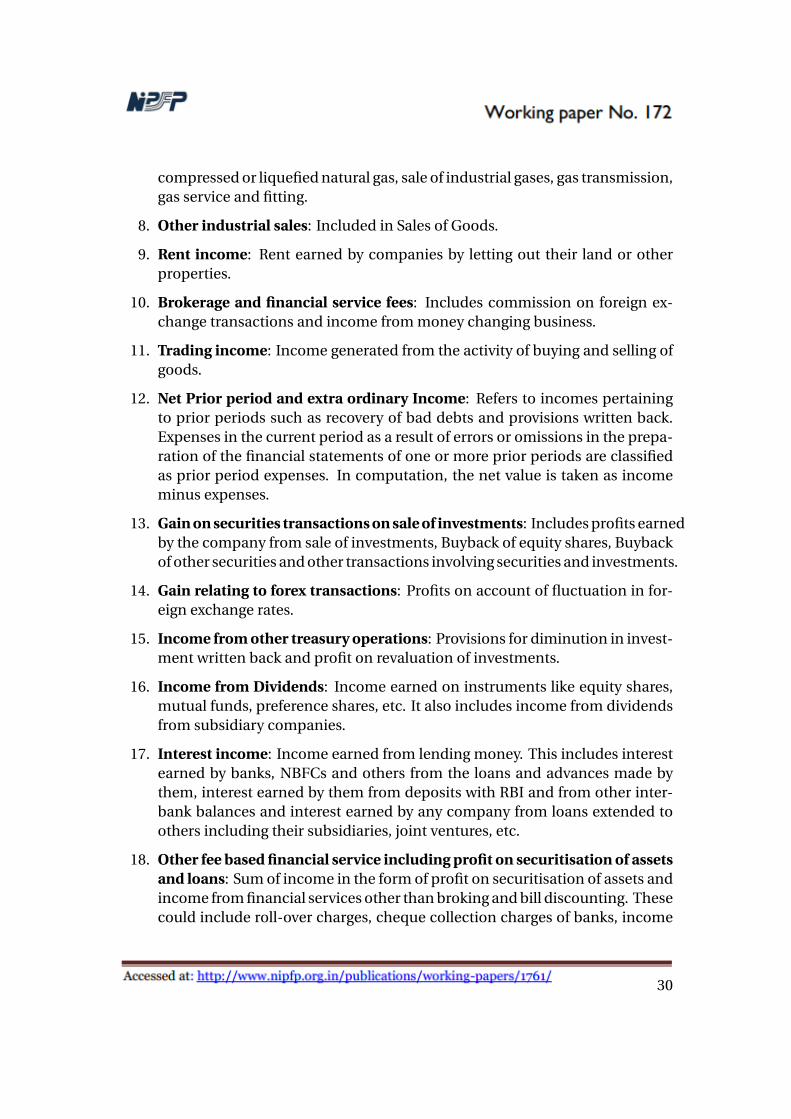
compressed or liquefied natural gas, sale of industrial gases, gas transmission,gas service and fitting.

8. Other industrial sales: Included in Sales of Goods.

9. Rent income: Rent earned by companies by letting out their land or otherproperties.

10. Brokerage and financial service fees: Includes commission on foreign ex-change transactions and income from money changing business.

11. Trading income: Income generated from the activity of buying and selling ofgoods.

12. Net Prior period and extra ordinary Income: Refers to incomes pertainingto prior periods such as recovery of bad debts and provisions written back.Expenses in the current period as a result of errors or omissions in the prepa-ration of the financial statements of one or more prior periods are classifiedas prior period expenses. In computation, the net value is taken as incomeminus expenses.

13. Gain on securities transactions on sale of investments: Includes profits earnedby the company from sale of investments, Buyback of equity shares, Buybackof other securities and other transactions involving securities and investments.

14. Gain relating to forex transactions: Profits on account of fluctuation in for-eign exchange rates.

15. Income from other treasury operations: Provisions for diminution in invest-ment written back and profit on revaluation of investments.

16. Income from Dividends: Income earned on instruments like equity shares,mutual funds, preference shares, etc. It also includes income from dividendsfrom subsidiary companies.

17. Interest income: Income earned from lending money. This includes interestearned by banks, NBFCs and others from the loans and advances made bythem, interest earned by them from deposits with RBI and from other inter-bank balances and interest earned by any company from loans extended toothers including their subsidiaries, joint ventures, etc.

18. Other fee based financial service including profit on securitisation of assetsand loans: Sum of income in the form of profit on securitisation of assets andincome from financial services other than broking and bill discounting. Thesecould include roll-over charges, cheque collection charges of banks, income

30

from custodial services, depository services, transaction charges or portfoliomanagement fees, etc.

19. Bill discounting: Income from transactions on bills of exchange, promissorynotes, etc. after deducting some amount from the face value of the bill asdiscounting charges.

20. Income from leasing, hire purchase, lease adjustment: Income from leasingand hire purchase income, lease equalisation adjustment, share of profit inpartnership firms/subsidiaries/ joint ventures other companies.

21. Indirect taxes: Indirect taxes reported are excise duties, sales tax or valueadded tax, custom duties, service tax, municipal/local tax, octroi/entry tax,stamp duty, luxury tax or any other kind of indirect tax levied by the central,state or local governments.

22. Sales tax and VAT benefits: Monetary benefit obtained by the companies fromsales tax authorities, such as set off against its sales tax liability and where theset off amount is greater than the sales tax liability, the company may showthe excess set off as an income.

23. Other fiscal benefits and subsidies: Fiscal benefits other than export incen-tives, duty draw back, benefits derived by oil companies from the governmentand sales tax benefits.

24. Fiscal benefits to oil companies: Benefits announced by Government of In-dia’s deregulation policy of pricing & distribution of petroleum products fordismantling of administered price mechanism (APM).

25. Export incentives including duty draw back, etc: Includes duty drawbacks,excise rebates, import licenses, concession in import duty and tax exemptionsunder the Income Tax Act.

26. Change in stock: Defined as change in stock of finished and semi-finishedgoods less opening stock of finished and semi-finished goods.

27. Raw materials, stores, spares: Sum of the expenses incurred on (a) raw ma-terials and on (b) stores, spares and tools consumed. They also cover sundrysupplies, maintenance stores, components, tools, jigs, and other similar equip-ment.

28. Purchase of finished goods: Includes purchase of finished by manufacturingcompanies, besides selling their own products.

29. Royalties, technical know-how, etc.: Sum total of Royalty, Technical know-how fees and License fees.

31

30. Rent, lease rent, etc.: Includes all types of rent, lease rents, finance lease rentsand operating lease rent.

31. Repairs and maintenance, etc.: Sum of Repairs and maintenance of build-ings, plant and machinery, vehicles and others.

32. Insurance premium paid, etc.: Amount of insurance premium paid on theassets of the company, on goods in transit and on key persons of the company.

33. Selling and distribution expenses: Expenditure on advertising, marketingand distribution.

34. Communications expenses: Cost incurred by the company on telephone,telegram, postage, fax, satellite, Internet services and other information tech-nology services.

35. Wealth tax: Provision for tax on the benefits derived from ownership of prop-erty. The tax is paid on the same property on its market value, whether or notsuch property yields any income.

36. Research and development expenses: Current expenses incurred and reportedby the company on research and development. It does not include any capitalexpenditure on research and development

37. Paid up equity capital: Paid up equity capital of the company.

32

D GVA in the Manufacturing sector, 2001-02–2014-15

GVA of XBRL filing companies 2002-2015, (Current prices, Rs. Crore)Year Output Net Taxes Int. Cons. GVA Count Gr. rate

1 2001-02 786059.38 80415.32 503834.99 201809.07 2894 -2 2002-03 893296.28 81477.88 602864.4 208954 2943 3.543 2003-04 1038973.6 94867.1 681966.27 262140.23 2928 25.454 2004-05 1266802.57 108892.44 879184.74 278725.39 3068 6.335 2005-06 1497085.69 120444.56 1075733.25 300907.88 3298 7.966 2006-07 1864666.41 134918.24 1322344.78 407403.39 3351 35.397 2007-08 2187870.82 140227.6 1559260.42 488382.8 3601 19.888 2008-09 2481138.44 75514.28 1827775.64 577848.52 3807 18.329 2009-10 2677288.33 120570.92 1962169.86 594547.55 3800 2.89

10 2010-11 3217555.54 142367.53 2432173.89 643014.12 3545 8.1511 2011-12 3798458.31 109695.63 2930897.15 757865.53 3479 17.8612 2012-13 4194934.27 129829.73 3255367.85 809736.69 3465 6.8413 2013-14 4317499.38 156324.06 3294421.66 866753.66 3073 7.0414 2014-15 3923854.14 208869.57 2858576.69 856407.88 2186 −1.19

GVA of XBRL filing companies based on NIC 2008 (10-33) classification, 2002-2015,(Current prices, Rs. Crore)

Year Output Net Taxes Int. Cons. GVA Count Gr. rate1 2001-02 695580.16 71549.67 435245.09 188785.4 2430 -2 2002-03 779648.69 70834.96 517120.7 191693.03 2445 1.543 2003-04 891914.67 79574.82 571881.89 240457.96 2412 25.444 2004-05 1074405.26 86775.28 734833.41 252796.57 2601 5.135 2005-06 1256628.41 89227.91 889379.05 278021.45 2789 9.986 2006-07 1537352.69 96681.43 1074845.19 365826.07 2838 31.587 2007-08 1828748.45 98006.28 1285960.19 444781.98 3072 21.588 2008-09 2070944.77 15591.45 1540208.92 515144.4 3250 15.829 2009-10 2218512.45 74708.81 1596091.28 547712.36 3268 6.32

10 2010-11 2653159.24 91007.66 1977049.37 585102.21 3076 6.8311 2011-12 3127739.71 57595.23 2385915.33 684229.15 3017 16.9412 2012-13 3455694.75 78945.9 2632457.78 744291.07 3010 8.7813 2013-14 3645458.84 111350.47 2734001.77 800106.6 2684 7.5014 2014-15 3264340.47 167792.18 2323662.07 772886.22 1915 −3.40

33

References

CSO (2010) New series of National accounts statistics (Base Year 2004-05), Ministry of Statis-tics and Programme Implementation Government of India, National Accounts Division,New Delhi

CSO (2011) Instructions to Field Officials on Annual Survey of Industries: Concepts, Defini-tions and Procedures, Ministry of Statistics and Programme Implementation Governmentof India, Field Operation Division, Central Statistics Office, (IS Wing), New Delhi

CSO (2015a) No room for doubts on new GDP numbers, Economic and Political Weekly, Vol.L, No. 16, April 18th, pp. 86-89

CSO (2015b) Final Report of the Sub-Committee on Private Corporate Sector including PPPs,National Accounts Division, Ministry of Statistics and Programme Implementation, Gov-ernment of India, New Delhi

CSO (2015c) Press Note on Provisional estimates of annual National Income 2014-15 andQuarterly estimates of Gross Domestic Product for the fourth quarter (Q4) 2014-15, NationalAccounts Division, Ministry of Statistics and Programme Implementation, Government ofIndia, New Delhi

CSO (2015d) Changes in methodology and data sources in the new series of National AccountsBase Year 2011-12, National Accounts Division, Ministry of Statistics and Programme Imple-mentation, Government of India, New Delhi

Dholakia, Ravindra H. (2015) Double deflation method and growth in manufacturing: Com-ment, Economic and Political Weekly, Vol. L, No. 41, 10th October, pp. 88-90

EPW, Editorial (2015) Some answers, some questions, Economic and Political Weekly, Vol.L, No. 6, Feb 7th, pp. 7-8

EPW, Editorial (2015a) GDP Numbers: More puzzles, more confusion, Economic and Polit-ical Weekly, Vol. L, No. 8, Feb 21st, pp. 7

EPW Research Foundation (2015) New series of National Accounts: A review, Economic andPolitical Weekly, Vol. L, No. 7, Feb 14th, pp. 74-78

Goldar, Bishwanath (2015) Growth in gross value added of Indian manufacturing, 2011-12Series vs 2004-05 series, Economic and Political Weekly, Vol. L, No. 20, May 23rd, pp. 10-13

Mazumdar, Surajit (2015) Manufacturing growth in the new GDP series, Economic and Po-litical Weekly, Vol. L, No. 24, June 13th, pp. 120-121

Nagaraj, R (2015a) Seeds of doubt on new GDP numbers Private corporate sector overesti-mated?, Economic and Political Weekly, Vol. L, No. 13, March 28th, pp. 14-17

34

Nagaraj, R (2015b) Seeds of doubt remain: A reply to CSO’s rejoinder, Economic and PoliticalWeekly, Vol-L, No. 18, May 8th , pp. 64-66

Nagaraj, R (2015c) Growth in GVA of Indian manufacturing, Economic and Political Weekly,Vol-L, No. 24, June 13th, pp. 117-120

Nagaraj, R (2015d) Size and structure of India’s Private corporate sector, Economic and Po-litical Weekly, Vol-L, No. 45, Nov 7th., pp. 41-47

Rajakumar, J Dennis (2015) Private corporate sector in new NAS series: Need for a freshlook, Economic and Political Weekly, Vol-L, No. 29, July 18th, pp. 149-153

Rajakumar, J Dennis & S.L Shetty (2015) Gross value added: Why not the double deflationmethod for estimation, Economic and Political Weekly, Vol-L, No. 33, August 15th, pp. 78-81

Rao, KGK Subba (2015) Mystery of private corporate savings, Economic and Political Weekly,Vol-L, No. 22, May 30th, pp. 158-162

SNA (2008) System of National Accounts, Published by the European Communities, Interna-tional Monetary Fund, Organization for Economic Co-operation and Development, UnitedNations and World Bank, New York

35

MORE IN THE SERIES

Bhanumurthy, N.R. et al., 2016. “Public Expenditure, Governance and Human Development: A case of Madhya Pradesh”, No. 171(July)

Jena P. R., K. K. Bhadra, S. Sikdar, 2016. “Search for Resources in a High Income State: A Study of State Finances in Sikkim”, No. 170(May).

Rao R. K., S. Tandon, 2016. "Revisiting the TaxCompliance problem using Prospect Theory”. No.169(Apr).

Amey Sapre,Indian Institute of Technology, Kanpuremail: amey@iitk.ac.in

Pramod Sinha, isConsultant, NIPFPemail:pramod.sinha@nipfp.org.in

National Institute of Public Finance and Policy,18/2, Satsang Vihar Marg,

Special Institutional Area (Near JNU),

New Delhi 110067

Tel. No. 26569303, 26569780, 26569784Fax: 91­11­26852548

www.nipfp.org.in