indiana lake water quality assessment report for 2004 - 2008
TRANSCRIPT

Indiana Lake Water Quality Assessment Report For 2004 - 2008
Prepared by: Laura A. Montgrain and William W. Jones School of Public & Environmental Affairs
Indiana University Bloomington, Indiana
Prepared for: Indiana Department of Environmental Management
Office of Water Quality Indianapolis, Indiana
June 2009


i Lake Water Quality Assessment for 2004 - 2008
Acknowledgments
This report was written by Laura A. Montgrain and William W. Jones. Melissa Clark managed the laboratory and was QA/QC Officer. The report represents four years of traversing the State of Indiana, reading maps, searching for lake access, extracting stuck trailers, seemingly endless washing of laboratory glassware, and most importantly, having the opportunity to visit and sample the beautiful and varied lakes of Indiana. This work required the dedicated efforts of many people. Therefore, it is with gratitude that we recognize the superb efforts of the following SPEA graduate students who conducted the lake sampling and laboratory analyses of the water samples: Chris Bobay, Kevin Bruce, Matthew Deaner, Ted Derheimer, Sheila Doshi, Lisa Fascher, David Fuente, Aaron Johnson, Emily Kara, Mark Lehman, Aaron McMahon, Selena Medrano, Erin Miller, John Moyer, Eva Olin, Thomas Parr, Rachel Price, Matthew Robinson, Moira Rojas, Sarah Sauter, Josh Tennan, Kim Vest, and Amanda Watson. This work was made possible by a grant from the U.S. EPA Section 319 Nonpoint Source Program administered by the Indiana Department of Environmental Management (IDEM). The IDEM Project Officers were Carol Newhouse and Laura Bieberich.

ii Indiana Water Quality Assessment, 2004-2008
Table of Contents Acknowledgments............................................................................................................................ i Table of Contents …………………………………………………………………………. ...... …ii INDIANA CLEAN LAKES PROGRAM .......................................................................................1
Lake Water Quality Assessment ..........................................................................................1 Water Quality Parameters Included in Lake Assessments ..................................................5
LAKE CLASSIFICATION .............................................................................................................6
Lake Origin Classification ...................................................................................................6 Trophic Classification ..........................................................................................................8 Trophic State Indices ...........................................................................................................9 The Indiana Trophic State Index..............................................................................9 The Carlson Trophic State Index ...........................................................................13 Ecoregion Descriptions ......................................................................................................13
METHODS ....................................................................................................................................15
Field Procedures.................................................................................................................15 Lab Procedures...................................................................................................................16 Ecoregion Analysis ............................................................................................................16 Statistical Analyses ............................................................................................................17 Basin Analysis .......................................................................................................17 Water Quality Analysis Through Time ..................................................................19 Comparison of Lake Types ....................................................................................19
RESULTS ......................................................................................................................................21
Ecoregion Analysis ............................................................................................................21 Basin Analysis ...................................................................................................................33 Water Quality Analysis Through Time ..............................................................................33 Comparison of Lake Types ................................................................................................38
DISCUSSION ................................................................................................................................53
Ecoregion Analysis ............................................................................................................53 Basin Analysis ...................................................................................................................55 Water Quality Analysis Through Time ..............................................................................59 Comparison of Lake Types ................................................................................................60
CONCLUSIONS............................................................................................................................63 REFERENCES ..............................................................................................................................65

1 Lake Water Quality Assessment for 2004 - 2008
INDIANA CLEAN LAKES PROGRAM The Indiana Clean Lakes Program was created in 1989 as a program within the Indiana Department of Environmental Management's (IDEM) Office of Water Management. The program is administered through a grant to Indiana University's School of Public and Environmental Affairs (SPEA) in Bloomington. The Indiana Clean Lakes Program is a comprehensive, statewide public lake management program having five components: 1. Public information and education 2. Technical assistance 3. Volunteer lake monitoring 4. Lake water quality assessment 5. Coordination with other state and federal lake programs. This document is a summary of lake water quality assessment results for 2004-2008. Lake Water Quality Assessment
The goals of the lake water quality assessment component include: (a) identifying water quality trends in individual lakes, (b) identifying lakes that need special management, and (c) tracking water quality improvements due to industrial discharge and runoff reduction programs (Jones 1996).
Public lakes are defined as those that have navigable inlets or outlets or those that exist on or adjacent to public land. Only public lakes that have boat trailer access from a public right-of-way are generally sampled in this program. Sampling occurs in July and August of each year to coincide with the period of thermal stratification (Figure 1) and the period of poorest annual water quality in lakes. Most Indiana lakes having maximum depths of 16 to 23 feet or greater undergo thermal stratification during the summer. As the sun and air temperatures warm the surface water of a lake the warmed water becomes less dense. This “lighter” water floats on top of the cold, denser water at the lake’s bottom. Summer wind and waves may not be strong enough to overcome the density differences between the surface and bottom waters and thermal stratification occurs. In a stratified lake, the surface waters (epilimnion) circulate and mix all summer while the bottom waters (hypolimnion) may stagnate because they are isolated from the surface. Thus, water characteristics in the epilimnion and hypolimnion of a given lake may be significantly different during stratification.
To account for potential differences between the epilimnion and hypolimnion of stratified lakes, water samples are collected from one meter below the surface and from one to two meters above the bottom. In addition, dissolved oxygen and temperature are measured at one-meter intervals from the surface to the bottom of each lake.
In the past, approximately 80 lakes were assessed each summer proceeding geographically through the state to minimize travel costs. Though 79 lakes were sampled in 2008, no lakes were sampled in 2007 and only 38 lakes were sampled in 2006. There are two reasons for this recent decrease in the number of CLP lakes sampled. First, a new sampling scheme was

2 Indiana Water Quality Assessment, 2004-2008
adopted in 2006. In the past, sampling occurred at one site on each lake, and was positioned over the deepest part of the lake. However, multi-basin lakes were studied in 2006 and 2008, with sampling occurring at three sites per lake. Site one was located at the deepest part of the lake, and sites two and three were located in other (usually shallower) basins. Sampling three sites per lake as opposed to one site per lake may provide a more accurate description of water quality in multi-basin lakes since the deepest part of a lake may not always be representative of the entire lake. However, an increase in the sampling effort per lake inevitably led to a decrease in the number of lakes sampled per season. To determine whether sampling more sites per lake does indeed provide a more accurate description of water quality, a statistical comparison of the two sampling schemes (one site per lake and three sites per multi-basin lake) was performed and can be found later in this report.
Second, sampling efforts were devoted to the U.S. EPA’s National Lakes Assessment in
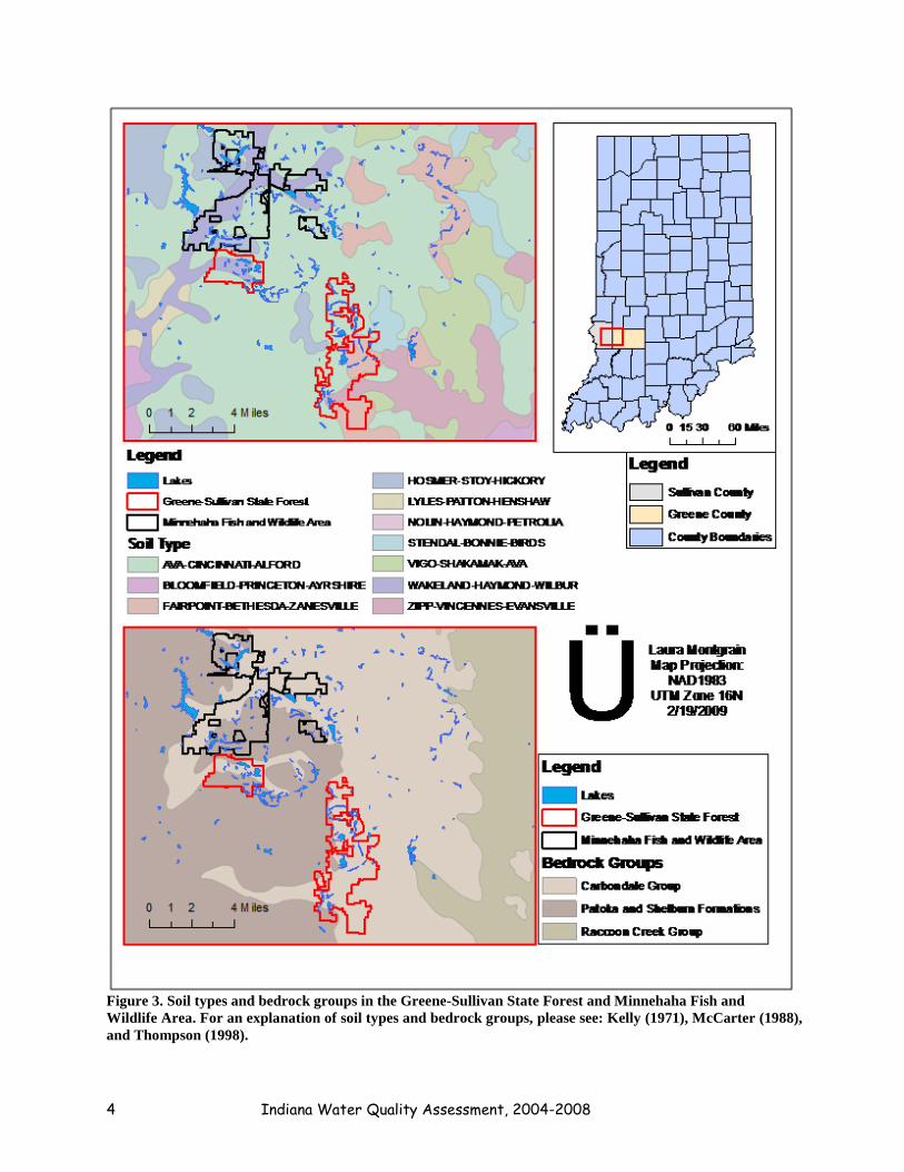
the summer of 2007. Therefore, sampling for the CLP was suspended during the 2007 season. In addition, a greater emphasis was placed on sampling coal mine lakes in 2008 than in past sampling seasons. In fact, 51 of the 79 lakes that were sampled in 2008 were coal mine lakes, where only the deepest site was sampled per lake. Sampled coal mine lakes are located in the Green-Sullivan State Forest and the Minnehaha Fish and Wildlife Area (Figure 2). These coal mine lakes have unique water quality characteristics due to local soil and geological factors (Figure 3) and on the way in which they were formed. To highlight the unique characteristics of coal mine lakes, a comparison of the water quality of coal mine lakes, impoundments, and natural lakes is found later in this report. Of the 69 lakes sampled in 2008, 51 were sampled at only the deepest site. The remaining 18 CLP lakes were sampled at multiple sites per lake.
Figure 1. Summer thermal stratification prevents lake mixing because the cool waters of the hypolimnion are much denser than the warm waters of the epilimnion. Epilimnetic waters circulate with the wind but do not mix until the lake cools again in the fall. Adapted from: Olem and Flock, 1990.

3 Lake Water Quality Assessment for 2004 - 2008
Figure 2. Greene-Sullivan State Forest and Minnehaha Fish and Wildlife Area.
4 Indiana Water Quality Assessment, 2004-2008
Figure 3. Soil types and bedrock groups in the Greene-Sullivan State Forest and Minnehaha Fish and Wildlife Area. For an explanation of soil types and bedrock groups, please see: Kelly (1971), McCarter (1988), and Thompson (1998).

5 Lake Water Quality Assessment for 2004 - 2008
Water Quality Parameters Included in Lake Assessments
Monitoring lakes requires many different parameters to be sampled. The parameters analyzed in this assessment include:
Phosphorus Phosphorus is an essential plant nutrient and most often controls aquatic plant (algae and macrophyte) growth in freshwater. It is found in fertilizers, human and animal wastes, and yard waste. There is no atmospheric (vapor) form of phosphorus. Because there are few natural sources of phosphorus and the lack of an atmospheric cycle, phosphorus is often a limiting nutrient in aquatic systems. This means that the relative scarcity of phosphorus may limit the ultimate growth and production of algae and rooted aquatic plants. Therefore, management efforts often focus on reducing phosphorus input to a receiving waterway because: (a) it can be managed, and (b) reducing phosphorus can reduce algae production. Two common forms of phosphorus are:
Soluble reactive phosphorus (SRP) – SRP is dissolved phosphorus readily usable by algae. SRP is often found in very low concentrations in phosphorus-limited systems where the phosphorus is tied up in the algae and cycled very rapidly. Sources of SRP include fertilizers, animal wastes, and septic systems. Total phosphorus (TP) – TP includes dissolved and particulate forms of phosphorus. TP concentrations greater than 0.03 mg/L (or 30µg/L) can cause algal blooms in lakes and reservoirs.
Nitrogen Nitrogen is an essential plant nutrient found in fertilizers, human and animal wastes, yard waste, and the air. About 80% of the atmosphere is nitrogen gas. Nitrogen gas diffuses into water where it can be “fixed” (converted) by blue-green algae to ammonia for algal use. Nitrogen can also enter lakes and streams as inorganic nitrogen and ammonia. Because nitrogen can enter aquatic systems in many forms, there is an abundant supply of available nitrogen in these systems. The three common forms of nitrogen are:
Nitrate (NO3-) – Nitrate is an oxidized form of dissolved nitrogen that is converted to
ammonia by algae under anoxic (low or no oxygen) conditions. It is found in streams and runoff when dissolved oxygen is present, usually in the surface waters. Ammonia (NH4
+) – Ammonia is a form of dissolved nitrogen that is readily used by algae. It is the reduced form of nitrogen and is found in water where dissolved oxygen is lacking such as in a eutrophic hypolimnion. Important sources of ammonia include fertilizers and animal manure. In addition, ammonia is produced as a by-product by bacteria as dead plant and animal matter are decomposed. Organic Nitrogen (Org N) – Organic nitrogen includes nitrogen found in plant and animal materials and may be in dissolved or particulate form. In the analytical procedures, total Kjeldahl nitrogen (TKN) was determined. Organic nitrogen is TKN minus ammonia.

6 Indiana Water Quality Assessment, 2004-2008
Light Transmission This measurement uses a light meter (photocell) to determine the rate at which light transmission is diminished in the upper portion of the lake’s water column. Another important light transmission measurement is determination of the 1% light level. The 1% light level is the water depth to which one percent of the surface light penetrates. The 1% light level is considered the lower limit of algal growth in lakes and this area and above is referred to as the photic zone. Dissolved Oxygen (D.O.) D.O. is the dissolved gaseous form of oxygen. It is essential for respiration of fish and other aquatic organisms. D.O. enters water by diffusion from the atmosphere and as a by-product of photosynthesis by algae and plants. Epilimnetic waters continually equilibrate with the concentration of atmospheric oxygen. Excessive algae growth can over-saturate (greater than 100% saturation) the water with D.O when rate of photosynthesis production is greater than the rate of oxygen diffusion to the atmosphere. Hypolimnetic D.O. concentration is typically low as there is no mechanism to replace oxygen that is consumed by respiration and decomposition. Fish need at least 3-5 mg/L of D.O. to survive. Secchi Disk Transparency Secchi disk transparency refers to the depth to which the black and white Secchi disk can be seen in the lake water. Water clarity, as determined by a Secchi disk, is affected by two primary factors: algae and suspended particulate matter. Particulates (soil or dead leaves) may be introduced into the water by either runoff or sediments already on the bottom of the lake. Erosion from construction sites, agricultural lands, and riverbanks all lead to increased runoff. Bottom sediments may be resuspended by bottom-feeding fish such as carp, or by motorboats or strong winds in shallow lakes. Plankton Plankton are important members of the aquatic food web. Plankton includes algae (microscopic plants) and zooplankton (tiny shrimp-like animals that eat algae). Plankton are collected by filtering water through a very fine mesh net (63-micron openings = 63/1000 millimeter). The plankton net is towed up through the lake’s water column from the one percent light level to the surface. Blue-green algae are those that most often form nuisance blooms and their dominance in lakes may indicate poor water conditions. Chlorophyll a The plant pigments of algae consist of the chlorophylls (green color) and carotenoids (yellow color). Chlorophyll a is the most dominant chlorophyll pigment. Thus, chlorophyll a is often used as a direct estimate of algal biomass.

7 Lake Water Quality Assessment for 2004 - 2008
LAKE CLASSIFICATION There are many factors that influence the condition of a lake including physical dimensions (morphometry), nutrient concentrations, oxygen availability, temperature, light, and fish species. In order to simplify the analysis of lakes, there are a variety of lake classifications that are used. Lake classifications serve to aid in the decision-making process, in prioritizing, and in creating public awareness. Lakes can be classified based on their origin, thermal stratification regime, or on trophic status. Lake Origin Classification Hutchinson (1957) classified lakes according to how they were formed which resulted in 76 different classifications; the following are important to Indiana. Glacial Lakes As the ice sheets moved south and then receded, they created several types of lakes including scour lakes and kettle lakes. Scour lakes are formed when the sheet moves over the land creating a groove in the surface of the earth which later fills with meltwater. Kettle lakes are formed when large chunks of ice deposited by the glacier leave depressions in the landscape that fill in with water. The majority of lakes in Indiana are kettle lakes including Lake Tippecanoe, the deepest lake (123 feet), and Lake Wawasee, the largest lake (3,410 acres). Glacial lakes in Indiana are primarily in the north and found between the western Valparaiso Morainal Area and the eastern Steuben Morainal Area (Figure 4). Solution Lakes Solution lakes form when water collects in basins formed by the solution of limestone found in regions of karst topography. These lakes tend to be circular and are primarily found in the Mitchell Plain of southern Indiana. Oxbow Lakes Oxbow lakes are formed from former river channels that have been isolated from the original river channel due to deposition of sedimentation or erosion. Oxbow lakes can be found throughout the State of Indiana. Artificial Lakes Artificial lakes are created by humans due to excavation of a site or to damming a stream or river. Artificial lakes include ponds, strip pits, borrow pits, and reservoirs (Jones 1996). Reservoirs are typically elongate with many branches representing the tributaries of the former stream or river. Strip pits are found in southwestern Indiana where coal mines are located. All types of artificial lakes may be found throughout the State of Indiana.

8 Indiana Water Quality Assessment, 2004-2008
Figure 4. The Lake Michigan, Saginaw, and Erie lobes of the most recent glacial episode affected northern
Indiana. Glacial lakes are thus limited to this part of the state.
Trophic Classification Trophic state is an indication of a lake’s nutritional level or biological productivity. The following definitions are used to describe the tropic state of a lake: Oligotrophic - lakes with clear waters, low nutrient levels (total phosphorus < 6 µg/L), supports few algae, hypolimnion has dissolved oxygen, and can support salmonids (trout and salmon). Mesotrophic - water is less clear, moderate nutrient levels (total phosphorus 10-30 µg/L), support healthy populations of algae, less dissolved oxygen in the hypolimnion, and lack of salmonids. Eutrophic - water transparency is less than 2 meters, high concentrations of nutrients (total phosphorus > 35 µg/L), abundant algae and weeds, lack of dissolved oxygen in the hypolimnion during the summer.

9 Lake Water Quality Assessment for 2004 - 2008
Hypereutrophic - water transparency less than 1 meter, extremely high concentrations of nutrients (total phosphorus > 80 µg/L), thick algal scum, dense weeds.
Eutrophication is the biological response observed in a lake caused by increased nutrients, organic material, and/or silt (Cooke et al., 1993). Nutrients enter the lake through runoff or through eroded soils to which they are attached. Increased nutrient concentrations stimulate the growth of aquatic plants. Sediments and plant remains accumulate at the bottom of the lake decreasing the mean depth of the lake. The filling-in of a lake is a natural process that usually occurs over thousands of years. However, this natural process can be accelerated by human activities such as increased watershed erosion and increased nutrient loss from the land. This cultural eutrophication can degrade a lake in as little as a few decades (Figure 5).
Although it is widely known that nutrients, especially phosphorus, are responsible for
increased productivity, the concentration of nutrients alone cannot determine the trophic state of a lake. Other factors such as the presence of algae and weeds aid in the determination of the trophic status, and other factors such as light and temperature impact the growth of algae and weeds.
Trophic State Indices Due to the complex nature and variability of water quality data, a trophic state index (TSI) is used to aid in the evaluation of water quality data. A TSI assigns a numerical value to different levels of standard water quality parameters. The sum of these points for all parameters in the TSI represents the standardized trophic status of a lake that can be compared in different years or can be compared to other lakes. When using a TSI for comparison, it is important to not neglect the actual data as these data may help in explaining other differences between lakes. As with any index, when the data are reduced to a single number for a TSI, some information is lost. The Indiana Trophic State Index
The original purpose of the Indiana State Tropic Index (ITSI) was to identify lakes with problems and to determine the reasons for complaints from lake users. The ITSI was not used to rank Indiana lakes until the mid 1970’s.
The ITSI consists of 10 metrics (Table 1), all of which must be evaluated in order to achieve an accurate score. The metrics include biological, chemical, and physical parameters. Water samples for nitrogen and phosphorus are collected and analyzed from both the epilimnion and the hypolimnion and the mean of the values is assigned a certain number of eutrophy points based on the mean concentration.

10 Indiana Water Quality Assessment, 2004-2008
Figure 5. Lake eutrophication. Adapted from Freshwater Foundation (1985).

11 Lake Water Quality Assessment for 2004 - 2008
Table 1. The Indiana Trophic State Index
Parameter and Range Eutrophy Points I. Total Phosphorus (μg/L)
A. At least 30 1 B. 40 to 50 2 C. 60 to 190 3 D. 200 to 990 4 E. 1000 or more 5
II. Soluble Phosphorus (μg/L)
A. At least 30 1 B. 40 to 50 2 C. 60 to 190 3 D. 200 to 990 4 E. 1000 or more 5
III. Organic Nitrogen (mg/L)
A. At least 0.5 1 B. 0.6 to 0.8 2 C. 0.9 to 1.9 3 D. 2.0 or more 4
IV. Nitrate (mg/L)
A. At least 0.3 1 B. 0.4 to 0.8 2 C. 0.9 to 1.9 3 D. 2.0 or more 4
V. Ammonia (mg/L)
A. At least 0.3 1 B. 0.4 to 0.5 2 C. 0.6 to 0.9 3 D. 1.0 or more 4
VI. Dissolved Oxygen:
Percent Saturation at 5 feet from surface A. 114% or less 0 B. 115% 50 119% 1 C. 120% to 129% 2 D. 130% to 149% 3
E. 150% or more 4

12 Indiana Water Quality Assessment, 2004-2008
Indiana Trophic State Index (continued) VII. Dissolved Oxygen:
Percent of measured water column with at least 0.1 ppm dissolved oxygen A. 28% or less 4 B. 29% to 49% 3 C. 50% to 65% 2 D. 66% to 75% 1 E. 76% 100% 0
VIII. Light Penetration (Secchi Disk)
A. Five feet or under 6 IX. Light Transmission (Photocell)
Percent of light transmission at a depth of 3 feet A. 0 to 30% 4 B. 31% to 50% 3 C. 51% to 70% 2 D. 71% and up 0
X. Total Plankton per liter of water sampled from a single vertical tow between the 1% light
level and the surface: A. less than 3,000 natural units/L 0 B. 3,000 - 6,000 natural units/L 1 C. 6,001 - 16,000 natural units/L 2 D. 16,001 - 26,000 natural units/L 3 E. 26,001 - 36,000 natural units/L 4 F. 36,001 - 60,000 natural units/L 5 G. 60,001 - 95,000 natural units/L 10 H. 95,001 - 150,000 natural units/L 15 I. 150,001 - 5000,000 natural units/L 20 J. greater than 500,000 natural units/L 25 K. Blue-Green Dominance: additional points 10
In the Indiana Trophic State Index, the total eutrophy points range from 0 to 75. Oligotrophic conditions are represented with a score of 0 to 15. Mesotrophic conditions score 16 to 30 points. Eutrophic conditions score 31 to 45. Hypereutrophic lakes have ITSI scores greater than 46. The higher the number of eutrophy points assigned to a parameter, the more likely that parameter is to support increased productivity in the lake. In general, eutrophy points range from 1 to 4. However, the scale is weighted based on the amount of plankton in the sample and the dominance of blue-green algae in the sample. Extra weight is given to the presence of algae due

13 Lake Water Quality Assessment for 2004 - 2008
to public perception of poor water quality. Eutrophy points for all metrics are then summed to produce the final ITSI score for the lake. The Carlson Trophic State Index
The Carlson Trophic State Index, developed by Bob Carlson (1977) is the most widely used TSI in the United States (Figure 6). Carlson used mathematical equations developed from the relationships observed between summer measurements of Secchi disk transparency, total phosphorus, and chlorophyll a in northern temperate lakes. Through Carlson’s TSI, one parameter, Secchi disk transparency, total phosphorus, or chlorophyll a, can be used to yield a TSI value for that lake. One parameter can also be used to predict the value of the other parameters. Values for the Carlson’s TSI range from 0 to 100 and each increase of 10 trophic points represents a doubling of algal biomass. Not all lakes exhibit the same relationship between Secchi disk transparency, total phosphorus, and chlorophyll a that Carlson’s lakes show; however, in these cases Carlson’s TSI gives valuable insight into the functioning of a particular lake. CARLSON'S TROPHIC STATE INDEX
Figure 6. The Carlson Trophic State Index.
Ecoregion Descriptions
When we say that ‘lakes are a reflection of their watershed’ we refer to not only land use
activities within the watershed that may influence lake characteristic, but also soil types, land slope, natural vegetation, climate, and other factors that define the ecological region or ecoregion. Omernik and Gallant (1988) defined ecoregions in the Midwest (Figure 7); the boundaries of these ecoregions were determined through the examination of land use, soils, and potential natural vegetation. These ecoregions have similar ecological properties throughout their range and these properties can influence lake water quality characteristics. The six ecoregions present in Indiana are described in Figure 7.

14 Indiana Water Quality Assessment, 2004-2008
Figure 7. Ecoregions of Indiana.
Central Corn Belt Plains (#54): This ecoregion covers 46,000 square miles of Indiana and Illinois. This ecoregion is primarily cultivated for feed crops, only 5% of the area is woodland. Crops and livestock are responsible for the nonpoint source pollution in this region. Eastern Corn Belt Plains (#55): This ecoregion covers 31,800 square miles of Indiana, Ohio, and Michigan. Hardwood forests can thrive in this area; 75% of the land is used for crop production. Few natural lakes or reservoirs are in this area.

15 Lake Water Quality Assessment for 2004 - 2008
Southern Michigan/Northern Indiana Till Plain (#56): This region covers 25,800 square miles of Michigan and Indiana. Oak-hickory forests are the dominant vegetation in this area; however, 25% of this area is urbanized. Huron/Erie Lake plain (#57): This region covers 11,000 square miles of Indiana, Ohio, and Michigan. This area used to be occupied by forested wetlands; however, the primary use is now farming and 10% of this region is urbanized. No lakes in this region were included in this study. Interior Plateau (#71): This area occupies 56,000 square miles from Indiana and Ohio down to Alabama. Land is used for pasture, livestock, and crops. Woodlands and forests remain in this area. There are many quarries and coal mines in this area; however, there are few natural lakes. Interior River Lowland (#72): This area covers 29,000 square miles in Indiana, Kentucky, Illinois, and Missouri. One third of this area is maintained as oak-hickory forest; other land uses include pasture, livestock, crops, timber, and coal mines. Water quality disturbances come from livestock, crops, and surface mining.
METHODS
Field Procedures
Water samples are collected from the epilimnion and hypolimnion, generally 1 meter below the surface and from 1-2 meters above the bottom of the lake. Water samples taken for soluble reactive phosphorus (SRP), total phosphorus (TP), nitrate (NO3
-), ammonia (NH4+), and
total Kjeldahl nitrogen (TKN) are collected by using a Kemmerer water sampling device. SRP is filtered in the field using a 1.2 µm glass fiber filter and a hand pump. Prior to sampling, the TP, nitrate/ammonia, and TKN bottles are acidified with 0.125 ml of sulfuric acid (H2SO4).
Dissolved oxygen (D.O.) is measured using a YSI Model 85 Temperature/Dissolved Oxygen/Conductivity Meter or a Hydrolab Quanta water quality monitoring instrument. Measurements are taken at 1-meter intervals through the water column to the lake bottom.
Secchi disk transparency measurements are determined by the depth at which the black and white disk is no longer visible in the water column. Light penetration is measured with a LiCor Spherical Quantum Sensor.
Plankton samples are collected with a tow net that is lowered to the 1% light level as
determined by the light meter. The water is filtered through a fine-mesh net (63-microns) that concentrates the plankton. The plankton are washed into an opaque bottle with ultra-pure water and Lugol’s solution is added to preserve the sample based on the volume of the sample (4 cc/100 ml).

16 Indiana Water Quality Assessment, 2004-2008
Chlorophyll a is collected with an integrated sampler that reaches to a 2-m depth. The apparatus is shut, retrieved, and poured into a pitcher. The sample is shaded and filtered with Whatman GF/F filter paper using a hand pump. The sample is filtered until the flow of water passing through the filter is minimal and the volume of sample filtered is recorded. The filter paper is removed, placed in a bottle, and surrounded by ice. Lab Procedures
SRP is determined using the ascorbic acid method and measured colormetrically on a spectrophotometer (APHA, et al. 1998). TP samples are digested in hot acid to convert particulate phosphorus to dissolved phosphorus. After pH adjustment, the samples are analyzed as for SRP. NO3
- and NH4+ samples are filtered in the lab using a 0.45 micron membrane filter and a
hand pump. This analysis is run on an Alpkem Flow Solution Model 3570 autoanalyzer (OI Analytical, 2000). TKN samples are first digested in hot acid before being analyzed on the autoanalyzer. One milliliter of plankton sample is transferred to a Sedgwick-Rafter Cell for identification and enumeration. Fifteen random fields are selected and the genera are identified at 100x magnification. For the Crustacea, the entire slide is examined under the 4x objective to count all organisms in the sample. Algae are reported as natural units, which records one colonial filament of multiple cells as one natural unit and one cell of a singular alga also as one natural unit. The number of organism per liter is then calculated. Plankton identifications were made according to: Ward and Whipple (1959), Prescott (1982), Whitford and Schumacher (1984), and Wehr and Sheath (2003).
Chlorophyll filters are placed in the freezer upon arriving to the lab. Once frozen, the filters are ground using 90% aqueous acetone to extract the chlorophyll and read on a spectrophotometer. Samples are corrected for pheophyton pigments.
All sampling techniques and laboratory analytical methods were performed in accordance with procedures in Standard Methods for the Examination of Water and Wastewater, 20th Edition (APHA, 1998). Ecoregion Analysis Using SigmaPlot, morphology and water quality parameters were summarized by ecoregion for all the lakes sampled between 2004 and 2008.

17 Lake Water Quality Assessment for 2004 - 2008
Statistical Analysis Basin Analysis As previously mentioned, the summers of 2006 and 2008 represented a change from sampling one site per lake to sampling multiple (typically three) sites per lake. Statistical analyses were performed using the SPSS software package to determine whether sampling three sites per lake offers a more accurate description of water quality in Indiana lakes than sampling one site per lake. In other words, analyses were performed to determine whether the deepest sites of Indiana lakes are representative of the lakes as a whole.
The water quality parameters that were analyzed were Secchi depth (m), percent of the
water column that is oxic, light transmission at three feet, one percent light level (ft), dissolved oxygen saturation at five feet, epilimnetic and hypolimnetic pH, alkalinity (mg/L), conductivity (µmhos), nitrate concentration (mg/L), ammonia concentration (mg/L), TKN concentration (mg/L), SRP concentration (mg/L), and TP concentration (mg/L), as well as chlorophyll a concentration (mg/L), plankton (#/L), blue-green algal dominance, ITSI, and Carlson’s TSI. Water quality data from 2006 and 2008 were aggregated, as climate data show relatively similar conditions during both sampling periods (Table 2). Table 2. National Weather Service climate data for the 2006 and 2008 sampling seasons.
Data were divided into two samples: the first sample represented water quality
parameters at site one for all the lakes sampled in 2006 and 2008 and the second sample represented water quality parameters at sites two and three combined for all the lakes sampled in 2006 and 2008. After graphing the distributions of data within each sample to determine normality (or non-normality), the two samples were compared using either a paired t test or a nonparametric Wilcoxon Signed-Rank test. If water quality data for each sample were normally distributed, a paired t test was used to compare the means of each sample for each parameter (Figure 8). However if water quality data for each sample were not normally distributed, but the distributions were of the same shape, a nonparametric Wilcoxon Signed-Rank test was used to compare the medians of each sample for each parameter (Figure 9). This is because the paired t test assumes normally-distributed data and is not robust to deviations from normality. The
Wind (MPH)
Avg. High
Avg. Low
Mean Total Daily Avg.
Avg. Speed
Fair Partly Cloudy
Cloudy Thunderstorm Heavy Rain
Light Rain
Fog Haze Rain
June 80.1 60.8 70.5 5.63 0.19 7.6 6 18 6 12 3 17 21 12 13July 85.3 68 76.7 3.98 0.13 8 10 15 6 7 2 16 22 21 9
August 83.4 66.6 75.1 3.01 0.1 7.6 8 11 12 7 3 15 20 16 103 Month Total N/A N/A N/A 12.6 N/A N/A 24 44 24 26 8 48 63 49 32
3 Month Average 82.9 65.1 74.1 4.21 0.14 7.7 8 15 8 9 3 16 21 16 11
June 82.8 63.5 73.2 8 0.27 9.4 3 20 7 19 6 17 13 1 9July 83.8 66.1 75 6.58 0.21 7.6 7 18 6 8 7 14 16 12 6
August 83.5 64.2 73.8 1.83 0.06 7.2 9 20 2 3 2 3 7 9 23 Month Total N/A N/A N/A 16.4 N/A N/A 19 58 15 30 15 34 36 22 17
3 Month Average 83.4 64.6 74.0 5.47 0.18 8.1 6 19 5 10 5 11 12 7 6
2008
2006Temperature (F) Precipitation
(inches)Number of days with the
following sky cover conditionsNumber of days with the following weather
conditionsMonth

18 Indiana Water Quality Assessment, 2004-2008
Wilcoxon Signed-Rank test on the other hand only assumes that the distributions of data from the two samples are of the same shape. The paired design was chosen because the analysis involved repeated measurements on the same lakes.
Figure 8. Histogram showing a normal distribution of data. For normally-distributed data, the parametric
paired t test was used to compare the two samples.
Figure 9. Histogram showing a non-normal distribution of data. For distributions that are skewed but of the same shape, as seen here, the Wilcoxon Signed-Rank nonparametric test was used to compare the two
samples.

19 Lake Water Quality Assessment for 2004 - 2008
Water quality analysis through time Data for each lake sampled between 2004 and 2008 were combined with all previous sampling records for each of these lakes. Two samples were then created from this data set: the first sample consisted of our earliest sampling records for each lake in the sample population that was sampled between 2004 and 2008. The second sample consisted of the most recent (2004-2008) sampling records for these same lakes. Table 3 shows an example of how sampling records for the same lake were divided into two samples. In this case, the earliest sampling record for Beaver Dam Lake corresponded to the year 1994. Table 3. Table showing how sampling records were assigned to two statistical samples for comparison. This table does not show all the parameters that were analyzed.
To determine whether the water quality of these lakes has changed over time, the two
samples were compared using paired t tests or nonparametric Wilcoxon Singed Rank tests, based on the distribution of the data (as explained earlier). Again, SPSS was used, and the paired design was chosen because the analysis involved repeated measurements on the same lakes. Parameters that were compared between the two samples were Secchi depth (m), light transmission at three feet (%), one percent light level (ft), dissolved oxygen saturation at five feet (%), percent of the water column that is oxic (%), chlorophyll a concentration, (mg/m3), plankton (#/L), blue-green algal dominance (%), average alkalinity (mg/L), average conductivity (µmhos), average pH, average nitrate concentration (mg/L), average ammonia concentration (mg/L), average TKN concentration (mg/L), average SRP concentration (mg/L), average TP concentration (mg/L), Carlson’s TSI, and Indiana TSI. For each lake sampled between 2004 and 2008, the change in Indiana TSI scores from the previous sampling occasion to the 2004-2008 sampling season was also determined.
Comparison of Lake Types All the lakes that were sampled between 2004 and 2008 were divided into three statistical samples, based on lake type (impoundments, natural lakes, or coal mine lakes). To determine whether water quality parameters varied by lake type, and to assess the unique characteristics of coal mine lakes, SPSS was used to compare the three samples. After graphing the distributions of data within each sample to determine normality (or non-normality) and shape, a Welch’s ANOVA or nonparametric Kruskal-Wallis test was used to compare water quality parameters between samples.
The Welch’s ANOVA was used to compare water quality parameters that had normally-
distributed data (Figure 10). This test is robust to unequal variances between samples. Parameters that were compared between samples with a Welch’s ANOVA were pH, Secchi disk TSI, Chlorophyll a TSI, Total phosphorus TSI, averaged Carlson’s TSI, and Indiana TSI. The
Sampling Record
Lake ID
Lake Name County Sample Year
Depth (m)
Surface Area (ha)
Secchi Depth (m)
1% Light Level (ft)
Plankton (#/L)
Average pH
Average TP (mg/L)
Carlson's TSI
Indiana TSI
87 515Beaver Dam Kosckiusko 1 1994 18.6 59.09 1 11 9188 7.95 0.297 51 39
1610 515Beaver Dam Kosckiusko 2 2008 18 59.09 0.85 8.2 19985 8.1 0.236 64 33

20 Indiana Water Quality Assessment, 2004-2008
Kruskal-Wallis test was used to compare parameters that had distributions of data that were non-normal but had the same shape between samples (Figure 11). Parameters that were compared between samples with a Kruskal-Wallis were maximum depth (m), surface area (ha), Secchi disk transparency (m), percent of the water column that is oxic (%), chlorophyll a concentration (mg/m3), nitrate concentration (mg/L), ammonia concentration (mg/L), TKN concentration (mg/L), and total phosphorus concentration (mg/L).
A significant result for a Welch’s ANOVA or Kruskal-Wallis test indicates that the mean (for Welch’s ANOVA) or median (for Kruskal-Wallis) of one or more samples is significantly different from the mean or median of the other samples. These tests do not indicate which particular samples differ from the others. Therefore, following the Welch’s ANOVA and Kruskal-Wallis tests, post hoc tests were performed to determine which lake type significantly differed from the others in terms of water quality. For the parameters that were compared between lake types using a Welch’s ANOVA (see above), the Games-Howell post hoc test was employed in SPSS. This test accommodates unequal sample sizes and unequal variances between samples, but requires normally-distributed data. For the parameters that were compared between lake types using a Kruskal-Wallis test (see above), Holm’s sequential Bonferroni procedure was used. This procedure accommodates unequal sample sizes, unequal variances between samples, and non-normal distributions of data.
Figure 10. Histogram showing data with normal distributions and unequal variances between samples. A
Welch’s ANOVA was used to compare data with this type of distribution.

21 Lake Water Quality Assessment for 2004 - 2008
Figure 11. Histogram showing data that had non-normal distributions, unequal variances between samples,
and similar shapes between samples. A Kruskal-Wallis was used to compare data with this type of distribution.
RESULTS
Compiled physical, chemical, and biological data of the 198 CLP lakes that were sampled from 2004 to 2008 are presented in the appendices (Appendix A (2004), Appendix B (2005), Appendix C (2006), Appendix D (2008). Appendix E shows the data for the 51 coal mine lakes that were sampled in 2008. The Indiana Water Resource (Clark 1980) and the Indiana Lakes Guide (IDNR 1993) were the sources of lake areas and depths; however, maximum lake depth was revised based on the maximum depth observed while sampling the lake. Ecoregion Analysis Morphometry From 2004-2008, the greatest number of CLP lakes sampled was in ecoregion 56 (132 lakes) and the fewest number of lakes sampled was in ecoregion 55 and 71 (7 lakes each). Ecoregion 71 had the largest median surface area of 667.8 ha (this ecoregion contains the very large Monroe reservoir) while ecoregion 72 had the smallest median surface area of 4.9 ha (Figure 12). Ecoregion 55 had the second largest median surface area (132.3 ha) of all the lakes that were sampled, and ecoregions 54 and 56 had median lake areas of 36 ha and 47.4 ha

22 Indiana Water Quality Assessment, 2004-2008
Surface Area
Ecoregion
54 55 56 71 72
Sur
face
Are
a (h
a)
0
1000
2000
3000
4000
5000
Figure 12. Box and whisker plot showing the distribution of surface areas among lakes by ecoregion. A short box indicates that there was little difference in surface area of the sample lakes whereas a long box shows that
lakes in the ecoregion varied greatly in size. Ecoregion 71 contains the very large Monroe Reservoir.
Maximum Depth
Ecoregion
54 55 56 71 72
Max
imum
Dep
th (m
)
0
5
10
15
20
25
30
Figure 13. Maximum depth by ecoregion.

23 Lake Water Quality Assessment for 2004 - 2008
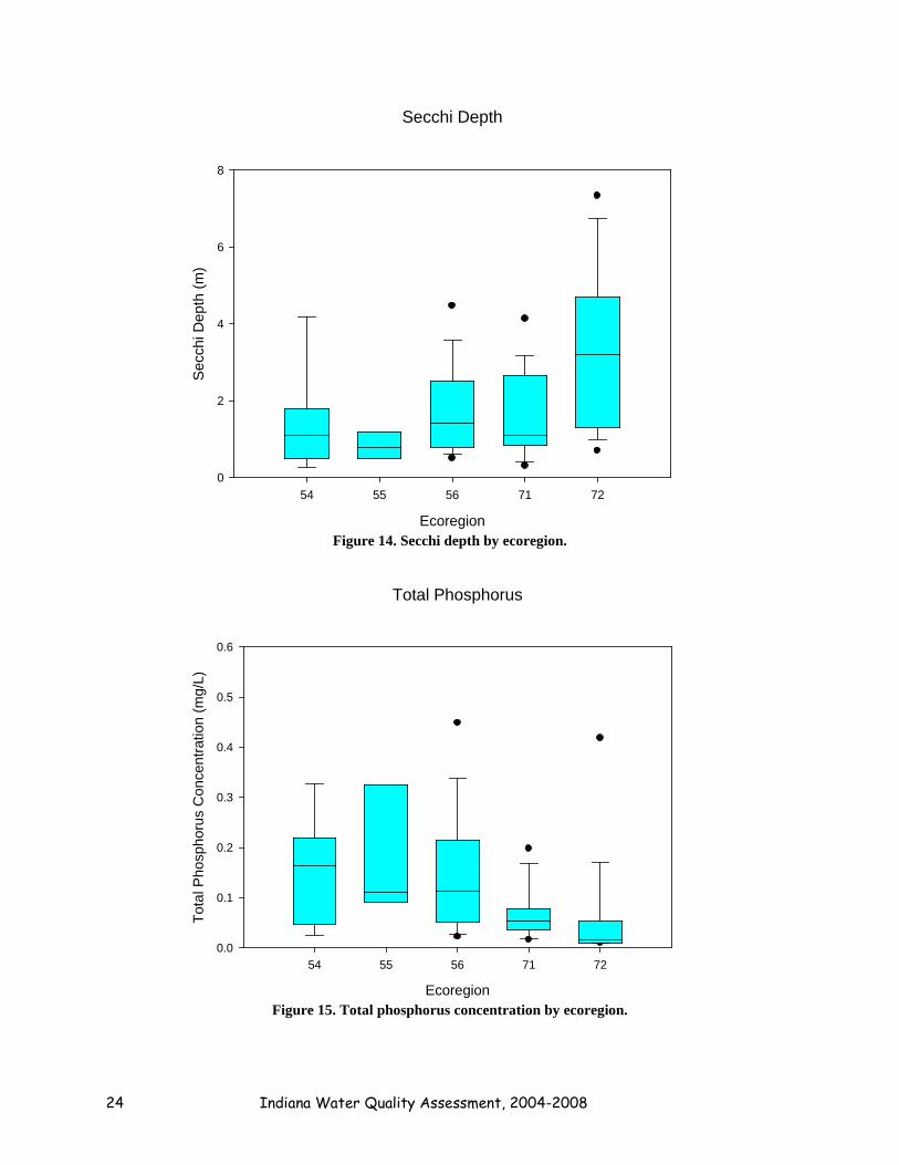
respectively. Ecoregion 56 had the deepest median lake at 11.6 m (Figure 13). The shallowest median lake depth was found in ecoregion 55 (6.1 m). The other ecoregions had median depths ranging from 6.7 m to 9.1 m. Secchi Disk Transparency Ecoregion 72 had the deepest median Secchi disk reading of 3.2 m (Figure 14). Ecoregion 56 had the second deepest median Secchi disk reading of 1.4 m. Ecoregion 54 and 71 both had median depths of 1.1 m. Ecoregion 55 had the shallowest median Secchi depth reading of 0.8 m. Total Phosphorus Ecoregion 54 had the highest median phosphorus concentration at 0.164 mg/L (Figure 15). Ecoregion 56 had a median phosphorus concentration of 0.113 mg/L and Ecoregion 55 had a median phosphorus concentration of 0.112 mg/L. Ecoregion 71 had a median phosphorus concentration of 0.054 mg/L. Ecoregion 72 had the lowest median phosphorus concentration of 0.017 mg/L. Chlorophyll a Ecoregion 55 had the highest median chlorophyll a concentration of 25.3 mg/m3 (Figure 16). Ecoregion 54 had the second highest median chlorophyll a concentration (13.36 mg/m3). Ecoregion 56 had a median chlorophyll a concentration of 7.78 mg/m3. Ecoregion 71 had a median chlorophyll a concentration of 4.55 mg/m3. Ecoregion 72 had the lowest median chlorophyll a concentration of 2.42 mg/m3. Nitrate Ecoregion 55 had the highest median nitrate concentration of 0.041 mg/L (Figure 17). Ecoregion 72 had a median nitrate concentration of 0.028 mg/L. Ecoregion 56 had a median concentration of 0.019 mg/L. Ecoregions 54 and 71 both had the lowest median concentration of 0.013 mg/L. Ammonia Ecoregion 56 had the highest median ammonia concentration of 0.580 mg/L (Figure 18). Ecoregion 55 had an ammonia concentration of 0.486 mg/L. Ecoregion 72 had a concentration of 0.400 mg/L. Ecoregion 54 had a median concentration of 0.183 mg/L. Ecoregion 71 had the lowest median ammonia concentration of 0.182 mg/L.
24 Indiana Water Quality Assessment, 2004-2008
Secchi Depth
Ecoregion
54 55 56 71 72
Sec
chi D
epth
(m)
0
2
4
6
8
Figure 14. Secchi depth by ecoregion.
Total Phosphorus
Ecoregion
54 55 56 71 72
Tota
l Pho
spho
rus
Con
cent
ratio
n (m
g/L)
0.0
0.1
0.2
0.3
0.4
0.5
0.6
Figure 15. Total phosphorus concentration by ecoregion.

25 Lake Water Quality Assessment for 2004 - 2008
Chlorophyll a
Ecoregion
54 55 56 71 72
Chl
orop
hyll
a co
ncen
tratio
n (m
g/m
3 )
0
20
40
60
80
100
Figure 16. Chlorophyll a concentration by ecoregion.
Nitrate
Ecoregion
54 55 56 71 72
Nitr
ate
conc
entra
tion
(mg/
L)
0.0
0.2
0.4
0.6
0.8
1.0
1.2
1.4
Figure 17. Nitrate concentration by ecoregion.

26 Indiana Water Quality Assessment, 2004-2008
Ammonia
Ecoregion
54 55 56 71 72
Am
mon
ia c
once
ntra
tion
(mg/
L)
0
2
4
6
8
10
Figure 18. Ammonia concentration by ecoregion.
Total Kjeldahl Nitrogen Ecoregion 56 had the highest median TKN concentration of 1.509 mg/L (Figure 19). Ecoregion 54 had a median concentration of 1.466 mg/L. Ecoregion 55 had a median concentration of 1.462 mg/L. Ecoregion 72 had a median concentration of 1.205 mg/L. Ecoregion 71 had the lowest median TKN concentration of 0.553 mg/L. Percent Water Column Oxic The median percent of the water column oxygenated in Ecoregion 72 was 54.5% which was the highest of the ecoregions (Figure 20). Ecoregion 55 had a median percentage of 53.1 while Ecoregion 54 had a median percentage of 51.5. Ecoregions 71 and 56 had median percentages of 47 and 40 respectively.

27 Lake Water Quality Assessment for 2004 - 2008
Total Kjeldahl Nitrogen (TKN)
Ecoregion
54 55 56 71 72
Tota
l Kje
ldah
l Nitr
ogen
con
cent
ratio
n (m
g/L)
0
1
2
3
4
5
Figure 19. TKN concentration by ecoregion.
Percent of the Water Column that is Oxic
Ecoregion
54 55 56 71 72
Per
cent
of t
he W
ater
Col
umn
that
is O
xic
(%)
0
20
40
60
80
100
120
Figure 20. Percent of the water column that is oxic by ecoregion.

28 Indiana Water Quality Assessment, 2004-2008
Indiana Trophic State Index The average trophic state value of all lakes sampled in an ecoregion during a sampling period of 5 years was used as a representative ITSI value for the ecoregion. There are five sampling periods in this data set: 1970’s, 1989-1993, 1994-1998, 1999-2003, and 2004-2008 (Figure 21). For all ecoregions, the general trend in eutrophy, according to the ITSI scores, tends to be towards mesotrophy. In addition, the 2004-2008 sampling period showed an increase in ITSI from the 1999-2003 sampling period for all ecoregions except ecoregions 71 and 72.
As Figure 21 shows, trends in eutrophy have consistently been very similar in ecoregions
54, 55 and 56. Ecoregion 54 typically showed the highest ITSI values through the years, except during the 1989-1993 period where Ecoregion 72 had the same ITSI value of 34. ITSI values for Ecoregion 54 ranged from 48 to 25. Since the 1970’s, the trophic state of Ecoregion 54 has changed from hypereutrophy (ITSI score of 48 in the 1970’s) to eutrophy (ITSI scores of 34, 31, and 28 in 1989-1993, 1994-1998, and 2004-2008 respectively). However, the 2004-2008 sampling period represents an increase in ITSI score from the 1999-2003 sampling period (from 25 to 28). ITSI values for Ecoregion 55 range from 40 to 24. Since the 1970’s the trophic state of Ecoregion 55 has changed from eutrophy (ITSI score of 40 in the 1970’s) to mesotrophy (ITSI scores of 30, 28, 24, and 26 in 1989-1993, 1994-1998, 1999-2003, and 2004-2008 respectively). Ecoregion 56 had ITSI scores that ranged from 34 to 23. Since the 1970’s the trophic state of Ecoregion 56 has also changed from eutrophy to mesotrophy.
Ecoregion 71 does not follow the same general eutrophy trends as ecoregions 54, 55 and
56. Although Ecoregion 71 remains mesotrophic (as in all previous sampling periods), ITSI scores decreased from 22 in 1989-1993 to 16 in 2004-2008. In addition, all of the ITSI scores for Ecoregion 71 are under 25. Ecoregion 72 is the only ecoregion that has shown a consistent decline in ITSI over time. The lowest ITSI score for Ecoregion 72 was 16 and was recorded in the 2004-2008 sampling period. This is considered to be a mesotrophic score. Carlson’s Trophic State Index The median trophic state value was obtained for each of the Carlson’s parameters in each ecoregion. Secchi Disk TSI. Ecoregion 55 had the highest median Carlson’s TSI score based on Secchi depth measurement (Figure 22). The median score was 63, which is considered to be eutrophic. Ecoregion 54 had a median Carlson’s TSI score of 59, Ecoregion 71 had a median Carlson’s TSI score of 58.5, and Ecoregion 56 had a median Carlson’s TSI of 55. All of these scores are considered to be eutrophic. Ecoregion 72 had the lowest median Carlson’s TSI score of 43, which is a mesotrophic score.

29 Lake Water Quality Assessment for 2004 - 2008
0
5
10
15
20
25
30
35
40
45
50
1970's 1989-1993 1994-1998 1999-2003 2004-2008
Mea
n Tr
ophi
c St
ate
Inde
x Sc
ore
Time Period
Ecoregion ITSI
5455567172
Figure 21. Indiana TSI scores by ecoregion across several sampling periods.
Chlorophyll a TSI. The highest median Carlson’s TSI score based on chlorophyll a concentrations was observed in Ecoregion 55 (Figure 23), which also had the highest Carlson’s TSI score based on Secchi depth. Ecoregion 55 had a score of 62 which is considered eutrophic. Ecoregion 54 had a median Carlson’s TSI score of 56, which is also eutrophic. Ecoregion 56 had a median Carlson’s TSI score of 51, which is considered mesotrophic, and Ecoregion 71 also had a mesotrophic median score (45.5). Ecoregion 72 had the lowest median Carlson’s TSI score of 39.5, which is mesotrophic.
Total Phosphorus TSI. Ecoregion 54 had the highest median Carlson’s TSI score based on total phosphorus concentration (Figure 24). The median score in ecoregion 54 was 78, indicating hypereutrophic conditions in this ecoregion. Ecoregion 56 had a median Carlson’s TSI score of 72.5 and Ecoregion 55 had a median Carlson’s TSI score of 72. Both these scores are also considered to be hypereutrophic. Ecoregion 71 had a median Carlson’s TSI score of 61.5, which is considered eutrophic, and Ecoregion 72 had the lowest median Carlson’s TSI score of 45, which is mesotrophic.

30 Indiana Water Quality Assessment, 2004-2008
Secchi Disk TSI
Ecoregion
54 55 56 71 72
Sec
chi D
isk
TSi
20
40
60
80
100
Figure 22. Secchi disk TSI by ecoregion.
Chlorophyll a TSI
Ecoregion
54 55 56 71 72
Chl
orop
hyll
a TS
I
20
40
60
80
100
Figure 23. Chlorophyll a TSI by ecoregion.

31 Lake Water Quality Assessment for 2004 - 2008
Total Phosphorus TSI
Ecoregion
54 55 56 71 72
Tota
l Pho
spho
rus
TSI
20
40
60
80
100
Figure 24. Total phosphorus TSI by ecoregion.
Averaged Score. All of the scores for a given lake were averaged, and the median of all the lakes in an ecoregion was obtained (Figure 25). The highest median Carlson’s TSI score was 63 and was found in Ecoregion 55. This score is considered eutrophic. Ecoregion 54 had a median Carlson’s TSI score of 59, and Ecoregion 56 had a median Carlson’s TSI score of 55. Both of these scores are also considered to be eutrophic. Ecoregion 71 had a median Carlson’s TSI of 54, which is also considered eutrophic, and Ecoregion 72 had the lowest median Carlson’s TSI of 41.5, which is considered to be mesotrophic. Comparison of ITSI and Carlson’s TSI Figure 26 compares the two trophic state indices for lakes sampled between 2004 and 2008. Nine of lakes sampled between 2004 and 2008 did not have ITSI and Carlson’s TSI scores. The ITSI indicates that 60 of the lakes sampled between 2004 and 2008 were oligotrophic while the Carlson’s index indicates that there were only 21 oligotrophic lakes sampled between 2004 and 2008. The ITSI and Carlson’s TSI showed similar numbers of mesotrophic lakes sampled between 2004 and 2008. The ITSI shows that there were 69 eutrophic lakes sampled between 2004 and 2008 while the Carlson’s TSI shows that there were 81 eutrophic lakes sampled during this same period. The Carlson’s TSI also shows that there were 35 hypereutrophic lakes sampled between 2004 and 2008, whereas the ITSI indicates that only 16 hypereutrophic lakes were sampled during this same period.

32 Indiana Water Quality Assessment, 2004-2008
Averaged Carlson's TSI
Ecoregion
54 55 56 71 72
Ave
rage
d TS
I
20
30
40
50
60
70
80
90
Figure 25. Averaged Carlson’s TSI by ecoregion.
21
115
81
35
60
103
69
16
0
20
40
60
80
100
120
140
Oligotrophic Mesotrophic Eutrophic Hypereutrophic
Num
ber o
f Lak
es
Trophic Classification
Comparison of Carlson's TSI and ITSI
Carlson's TSI
Indiana TSI
Figure 26. Comparison of Indiana TSI and Carlson’s TSI scores.

33 Lake Water Quality Assessment for 2004 - 2008
Basin analysis Recall that the purpose of these statistical analyses was to determine whether the deepest site of Indiana lakes is representative of the entire lakes. All the water quality data from 2006 and 2008 were aggregated and then divided into two samples. The first sample contained all the data from site one and the second sample contained all the combined data from sites two and three. For each parameter, the following hypotheses were tested: Ho: There is no difference between site one and the combined sites two and three. Ha: There is a difference between site one and the combined sites two and three.
For the SRP, TP, nitrogen, and TKN parameters, the non-normality of the distributions of data was due to a high frequency of data at the detection limits of the parameters. Table 4 shows the results of the Wilcoxon Signed-Rank or paired t tests for each parameter.
These results indicate that at the α = 0.05 level, site one was significantly different from sites two and three combined in terms of hypolimnetic ammonia (Z = -2.573, p = 0.008) and SRP concentration (Z = -2.977, p = 0.003). At the α = 0.1 level site one was significantly different from sites two and three combined in terms of chlorophyll a concentration (Z = -1.776, p = 0.076) and Carlson’s TSI (t = -1.850, p = 0.071). More precisely, site one had a higher concentration of hypolimnetic ammonia (Z = -2.573, p = 0.004) and hypolimnetic SRP (Z = -2.977, p = 0.0015) than sites two and three combined, and site one had a lower Carlson’s TSI (t = -1.850, p = 0.036) and concentration of chlorophyll a (Z = -1.776, p = 0.038) than sites two and three combined. Water quality analysis through time The purpose of these statistical analyses was to determine whether water quality in Indiana lakes has changed over time. Recall that data for each lake that was sampled between 2004 and 2008 were combined with all previous sampling records for each of these lakes, and two samples were created from this data set. The first sample consisted of the earliest sampling records for each lake that was sampled between 2004 and 2008. The second sample consisted of the most recent (2004-2008) sampling records for these same lakes. For each parameter, the following hypotheses were tested: Ho: There is no difference between the earliest sampling record and the most recent sampling record for all lakes sampled between 2004 and 2008. Ha: There is a difference between the earliest sampling record and the most recent sampling record for all lakes sampled between 2004 and 2008.
For the SRP, TP, nitrogen, and TKN parameters, the non-normality of the distributions of
data was due to a high frequency of data at the detection limits of the parameters. Table 5 shows the results of the Wilcoxon Signed-Rank or paired t tests for each parameter.

34 Indiana Water Quality Assessment, 2004-2008
Table 4. Basin analysis results. Bold data indicate statistical significance.
Parameter Mean of Site 1
Mean of Combined Sites 2 and 3
Mean difference (Site 1 – Combined Sites 2 and 3)
Test Test statistic
Significance (two-tailed)
Significance (one-tailed)
Secchi depth (m) 2.107 2.304 -0.197 Wilcoxon Singed-Rank Z = -0.943 p = 0.346 p = 0.173 Light transmission at 3 ft (%) 16.670 17.730 -1.060 Wilcoxon Singed-Rank Z = -0.314 p = 0.753 p = 0.377 1% light level (m) 13.870 13.550 0.320 Paired t test t = 0.204 p = 0.839 p = 0.420 D.O. saturation at 5 ft (%) 104.72 106.70 -1.98 Paired t test t = -0.463 p = 0.645 p = 0.323 Percent of the water column that is oxic 53.00 53.14 -0.14 Paired t test t = -0.017 p = 0.987 p = 0.494 Epilimnetic pH 8.465 8.519 -0.054 Paired t test t = -0.689 p = 0.493 p = 0.247 Hypolimnetic pH 7.594 7.650 -0.056 Paired t test t = -0.766 p = 0.447 p = 0.224 Epilimnetic conductivity (µmhos) 903.25 480.02 423.23 Paired t test t = 0.836 p = 0.407 p = 0.204 Hypolimnetic conductivity (µmhos) 330.09 343.63 -13.54 Paired t test t = -0.653 p = 0.517 p = 0.259 Epilimnetic alkalinity (mg/L) 142.61 140.03 2.58 Paired t test t = 0.390 p = 0.698 p = 0.349 Hypolimnetic alkalinity (mg/L) 182.52 173.40 9.12 Paired t test t = 1.220 p = 0.228 p = 0.114 Epilimnetic nitrate (mg/L) 0.288 0.346 -0.058 Wilcoxon Singed-Rank Z = -0.594 p = 0.553 p = 0.277 Hypolimnetic nitrate (mg/L) 0.120 0.300 -0.180 Wilcoxon Singed-Rank Z = -1.148 p = 0.251 p = 0.126 Epilimnetic ammonia (mg/L) 0.049 0.039 0.010 Wilcoxon Singed-Rank Z = 0.000 p = 1.000 p = 0.500 Hypolimnetic ammonia (mg/L) 1.145 0.716 0.429 Wilcoxon Singed-Rank Z = -2.673 p = 0.008 p = 0.004 Epilimnetic TKN (mg/L) 0.964 0.950 0.014 Wilcoxon Singed-Rank Z = -0.220 p = 0.826 p = 0.413 Hypolimnetic TKN (mg/L) 1.841 1.561 0.280 Wilcoxon Singed-Rank Z = -1.244 p = 0.213 p = 0.107 Epilimnetic SRP (mg/L) 0.011 0.010 0.001 Wilcoxon Singed-Rank Z = -0.350 p = 0.726 p = 0.363 Hypolimnetic SRP (mg/L) 0.125 0.059 0.066 Wilcoxon Singed-Rank Z = -2.977 p = 0.003 p = 0.0015 Epilimnetic TP (mg/L) 0.062 0.047 0.015 Wilcoxon Singed-Rank Z = -0.102 p = 0.919 p = 0.460 Hypolimnetic TP (mg/L) 0.158 0.111 0.047 Wilcoxon Singed-Rank Z = -1.571 p = 0.116 p = 0.058 Chlorophyll a (mg/m 3 ) 9.110 11.414 -2.304 Wilcoxon Singed-Rank Z = -1.776 p = 0.076 p = 0.038 Plankton (#/L) 18870.67 21353.43 -2482.76 Wilcoxon Singed-Rank Z = -0.080 p = 0.937 p = 0.469 Blue-green dominance (%) 52.06 50.52 1.54 Paired t test t = 0.260 p = 0.796 p = 0.398 Carlson’s TSI 48.653 52.673 -4.020 Paired t test t = -1.850 p = 0.071 p = 0.036 Indiana TSI 26.510 24.961 1.549 Paired t test t = 0.614 p = 0.542 p = 0.271

35 Lake Water Quality Assessment for 2004 - 2008
Table 5. Results of the water quality analysis through time.
Parameter Mean of Earliest Samples
Mean of 2004 - 2008 Samples
Mean difference (Earliest Sample - Current Sample)
Test Test statistic
Significance (two-tailed)
Significance (one-tailed)
Maximum Depth (m) 12.757 12.594 0.163 Paired t test t = 0.703 p = 0.483 p = 0.242 Surface area (ha) 131.4 137.7 -6.256 Wilcoxon Singed-Rank Z = -0.560 p = 0.575 p = 0.288 Secchi depth (m) 2.315 2.230 0.085 Wilcoxon Singed-Rank Z = -2.100 p = 0.036 p = 0.018 Light transmission at 3 ft (%) 36.18 23.82 12.36 Wilcoxon Singed-Rank Z = -7.120 p < 0.0005 p < 0.0005 1 % Light level (ft) 16.64 14.39 2.25 Wilcoxon Singed-Rank Z = -3.330 p = 0.001 p = 0.0005 D.O. Saturation at 5 ft (%) 99.57 104.90 -5.33 Paired t test t = -2.110 p = 0.036 p = 0.018 % of the water column that is oxic 66.71 53.08 13.63 Wilcoxon Singed-Rank Z = -5.970 p < 0.0005 p < 0.0005 Average pH 7.71 7.83 -0.122 Paired t test t = -1.738 p = 0.085 p = 0.043 Average conductivity (µmhos) 655.68 690.89 -35.21 Wilcoxon Singed-Rank Z = -0.675 p = 0.444 p = 0.222 Average alkalinity (mg/L) 200.33 202.41 -2.080 Wilcoxon Singed-Rank Z = -1.780 p = 0.074 p = 0.037 Average nitrate (mg/L) 0.861 0.157 0.704 Wilcoxon Singed-Rank Z = -9.170 p < 0.0005 p < 0.0005 Average ammonia (mg/L) 1.210 0.945 0.265 Wilcoxon Singed-Rank Z = -3.390 p = 0.001 p = 0.0005 Average TKN (mg/L) 2.045 1.773 0.272 Wilcoxon Singed-Rank Z = -3.210 p = 0.001 p = 0.0005 Average SRP (mg/L) 0.136 0.111 0.025 Wilcoxon Singed-Rank Z = -1.760 p = 0.078 p = 0.039 Average TP (mg/L) 0.16 0.154 0.006 Wilcoxon Singed-Rank Z = -1.410 p = 0.157 p = 0.079 Chlorophyll a (mg/m 3 ) 8.044 10.537 -2.493 Wilcoxon Singed-Rank Z = -3.010 p = 0.003 p = 0.0015 Plankton (#/L) 63278 19534 43744 Wilcoxon Singed-Rank Z = -1.740 p = 0.081 p = 0.041 Blue-green dominance (%) 51.8 51.2 0.62 Paired t test t = 0.211 p = 0.833 p = 0.417 Carlson’s TSI 45.29 46.74 -1.45 Paired t test t = -1.103 p = 0.274 p = 0.137 Indiana TSI 26.89 25.49 1.40 Paired t test t = 1.414 p = 0.159 p = 0.080

36 Indiana Water Quality Assessment, 2004-2008
These results indicate that at the α = 0.05 level, there was a difference between the earliest sampling record and the most recent sampling record for all lakes sampled between 2004 and 2008 for Secchi depth (Z = -2.100, p = 0.036), light transmission at three feet (Z = -7.120, p < 0.0005), one percent light level (Z = -3.330, p = 0.001), dissolved oxygen saturation at five feet (t = -2.110, p = 0.036), percent of the water column oxic (Z = -5.970, p < 0.0005), and average nitrate (Z = -9.170, p < 0.0005), ammonia (Z = -3.390, p = 0.001), TKN (Z = -3.210, p = 0.001), and chlorophyll a concentration (Z = -3.010, p = 0.003). At the α = 0.1 level, there was a significant difference between the earliest sampling record and the most recent sampling record for all lakes sampled between 2004 and 2008 for plankton (Z = -1.740, p = 0.081) and average pH (t = -1.738, p = 0.085), alkalinity (Z = -1.780, p = 0.074), and SRP (Z = -1.760, p = 0.078).
Specifically, the earliest sampling record had a greater Secchi depth (Z = -2.100, p =
0.018), light transmission at three feet (Z = -7.120, p < 0.0005), one percent light level (Z = -3.330, p = 0.0005), percent of the water column that is oxic (Z = -5.970, p < 0.0005), average nitrate (Z = -9.170, p < 0.0005), average ammonia (Z = -3.390, p = 0.0005), average TKN (Z = -3.210, p = 0.0005), average SRP (Z = -1.760, p = 0.039), and plankton (Z = -1.740, p = 0.041) than the most recent sampling record for all lakes sampled between 2004 and 2008. On the other hand, the earliest sampling record had a lower dissolved oxygen saturation at five feet (t = -2.110, p = 0.018), average pH (t = -1.738, p = 0.043), average alkalinity (Z = -1.780, p = 0.037), and chlorophyll a concentration (Z = -3.010, p = 0.0015) than the most recent sampling record for all lakes sampled between 2004 and 2008.
Also recall that for each lake sampled between 2004 and 2008, the change in Indiana TSI
scores from the earlier sampling date to the 2004-2008 sampling period was determined. An increase in TSI between the two sampling periods indicates an increase in conditions that can promote eutrophication. A decrease in TSI suggests a decrease in trophic state at a particular lake. Figure 27 shows the change in Indiana TSI scores for the lakes sampled between 2004 and 2008.
Change in Indiana Trophic State Index
Change in ITSI Points
-30 -25 -20 -15 -10 -5 0 5 10 15 20 25 30
Num
ber o
f Lak
es
0
10
20
30
40
50
Figure 27. Change in ITSI from previous to 2004-2008.
37 Lake Water Quality Assessment for 2004 - 2008
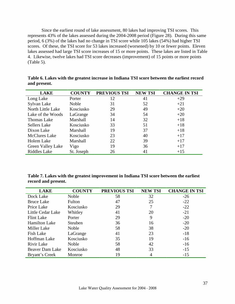
Since the earliest round of lake assessment, 80 lakes had improving TSI scores. This represents 43% of the lakes assessed during the 2004-2008 period (Figure 28). During this same period, 6 (3%) of the lakes had no change in TSI score while 105 lakes (54%) had higher TSI scores. Of these, the TSI score for 53 lakes increased (worsened) by 10 or fewer points. Eleven lakes assessed had large TSI score increases of 15 or more points. These lakes are listed in Table 4. Likewise, twelve lakes had TSI score decreases (improvement) of 15 points or more points (Table 5). Table 6. Lakes with the greatest increase in Indiana TSI score between the earliest record and present.
LAKE COUNTY PREVIOUS TSI NEW TSI CHANGE IN TSI Long Lake Porter 12 41 +29 Sylvan Lake Noble 31 52 +21 North Little Lake Kosciusko 29 49 +20 Lake of the Woods LaGrange 34 54 +20 Thomas Lake Marshall 14 32 +18 Sellers Lake Kosciusko 33 51 +18 Dixon Lake Marshall 19 37 +18 McClures Lake Kosciusko 23 40 +17 Holem Lake Marshall 22 39 +17 Green Valley Lake Vigo 19 36 +17 Riddles Lake St. Joseph 26 41 +15
Table 7. Lakes with the greatest improvement in Indiana TSI score between the earliest record and present.
LAKE COUNTY PREVIOUS TSI NEW TSI CHANGE IN TSI Dock Lake Noble 58 32 -26 Bruce Lake Fulton 47 25 -22 Price Lake Kosciusko 29 7 -22 Little Cedar Lake Whitley 41 20 -21 Flint Lake Porter 29 9 -20 Hamilton Lake Steuben 36 16 -20 Miller Lake Noble 58 38 -20 Fish Lake LaGrange 41 23 -18 Hoffman Lake Kosciusko 35 19 -16 Rivir Lake Noble 58 42 -16 Beaver Dam Lake Kosciusko 48 33 -15 Bryant’s Creek Monroe 19 4 -15

38 Indiana Water Quality Assessment, 2004-2008
43%
3%
54%
Summary of ITSI Score Changes
Improved
No Change
Worsened
Figure 28. Summary of Indiana TSI score changes from previous to 2004-2008.
Comparison of Lake Types Recall that several morphology and water quality parameters were compared between impoundments, natural lakes, and coal mine lakes. Data for all the lakes sampled between 2004 and 2008 were divided into three samples, based on lake type. For each morphology or water quality parameter, the following hypotheses were tested: Ho: The mean or median* parameter value of impoundments = the mean or median parameter value of natural lakes = the mean or median parameter value of coal mine lakes. Ha: The mean or median parameter value of at least one lake type differs from the mean or median parameter value of the other lake types. *The parameter of central tendency that was analyzed (mean or median) depended on the test that was employed. Welch’s ANOVA compares sample means and Kruskal-Wallis compares sample medians. Post hoc tests were employed after significant results were obtained with the Welch’s ANOVA or Kruskal-Wallis omnibus tests in order to determine which lake type(s) were significantly different from the others in terms of morphology and water quality. Table 8 outlines the results of the omnibus tests (Welch’s ANOVA and Kruskal-Wallis).

39 Lake Water Quality Assessment for 2004 - 2008
Table 8. Results of omnibus tests for the comparison of lake types.
Parameter Omnibus Test Omnibus Test Statistic
Omnibus Test Significance
Maximum depth (m) Kruskal-Wallis Chi-Square = 27.773 p < 0.0005 Surface Area (ha) Kruskal-Wallis Chi-Square = 60.010 p < 0.0005 Secchi depth (m) Kruskal-Wallis Chi-Square = 40.983 p < 0.0005 Percent of the water column that is oxic (%) Kruskal-Wallis Chi-Square = 22.037 p < 0.0005 Chlorophyll a concentration (mg/m3) Kruskal-Wallis Chi-Square = 18.794 p < 0.0005 pH Welch’s ANOVA F = 26.148 p < 0.0005 Nitrate (mg/L) Kruskal-Wallis Chi-Square = 0.799 p = 0.691 Ammonia (mg/L) Kruskal-Wallis Chi-Square = 11.203 p = 0.004 TKN (mg/L) Kruskal-Wallis Chi-Square = 21.569 p < 0.0005 TP (mg/L) Kruskal-Wallis Chi-Square = 65.280 p < 0.0005 Secchi disk TSI Welch’s ANOVA F = 24.145 p < 0.0005 Chlorophyll a TSI Welch’s ANOVA F = 12.108 p < 0.0005 Total phosphorus TSI Kruskal-Wallis Chi-Square = 65.274 p < 0.0005 Averaged Carlson’s TSI Welch’s ANOVA F = 38.491 p < 0.0005 Indiana TSI Welch’s ANOVA F = 25.973 p < 0.0005 Morphometry From 2004-2008, most of the lakes sampled were natural lakes (131 lakes) and the fewest number of lakes sampled were impoundments (28). Impoundments had the largest median surface area of 93.89 ha, and natural lakes had the second largest median surface area (49.2 ha). Coal mine lakes had the smallest median surface area (4.86 ha, Figure 29) of all the lake types that were sampled. In terms of surface area, after a significant Kruskal-Wallis result was obtained (Chi-square = 60.010, p < 0.0005, Table 8), the sequential Bonferroni procedure revealed that impoundments were not significantly different from natural lakes, but coal mine lakes were significantly different from both impoundments and natural lakes (Table 9). Therefore, as Figure 29 shows, coal mine lakes were significantly smaller than impoundments and natural lakes.
Coal mine lakes had the deepest median lake depth of 9.45 m, but natural lakes had a similar median depth of 9.4 m. Impoundments had the shallowest median depth (6.7 m) of all lake types sampled (Figure 30). In terms of maximum depth, after a significant Kruskal-Wallis result was obtained (Chi-square = 27.773, p < 0.0005, Table 8), the sequential Bonferroni procedure revealed that all lake types were significantly different from one another (Table 9). Secchi Disk Transparency Coal mine lakes had the deepest median Secchi disk reading of 3.3 m, whereas natural lakes and impoundments had median Secchi disk readings of 1.5 m and 1.1 m, respectively (Figure 31). After a significant Kruskal-Wallis result was obtained (Chi-square = 40.983, p < 0.0005, Table 8), the sequential Bonferroni procedure revealed that all lake types were significantly different from one another in terms of Secchi disk transparency (Table 9).

40 Indiana Water Quality Assessment, 2004-2008
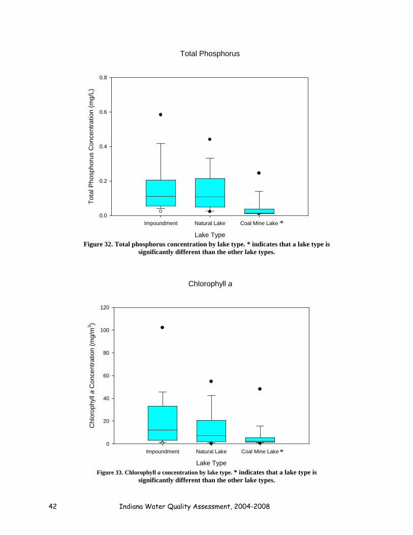
Total Phosphorus Impoundments had the highest median phosphorus concentration of 0.112 mg/L (Figure 32). Natural lakes had a median phosphorus concentration of 0.108 mg/L and coal mine lakes had the lowest median phosphorus concentration of 0.014 mg/L. In terms of total phosphorus concentration, after a significant Kruskal-Wallis result was obtained (Chi-square = 65.280, p < 0.0005, Table 8), the sequential Bonferroni procedure revealed that impoundments were not significantly different from natural lakes, but coal mine lakes were significantly different from both impoundments and natural lakes (Table 9). Therefore, as Figure 32 shows, coal mine lakes had significantly lower total phosphorus concentrations than impoundments and natural lakes. Chlorophyll a Impoundments had the highest median chlorophyll a concentration of 12.05 mg/m3 (Figure 33). Natural lakes had a median chlorophyll a concentration of 7.14 mg/m3 and coal mine lakes had the lowest median chlorophyll a concentration of 2.33 mg/m3. In terms of chlorophyll a concentration, after a significant Kruskal-Wallis result was obtained (Chi-square = 65.280, p < 0.0005, Table 8), the sequential Bonferroni procedure revealed that impoundments were not significantly different from natural lakes, but coal mine lakes were significantly different from both impoundments and natural lakes (Table 9). Therefore, as Figure 33 shows, coal mine lakes had significantly lower chlorophyll a concentrations than impoundments or natural lakes.
Surface Area
Lake Type
Impoundment Natural Lake Coal Mine Lake
Sur
face
Are
a (H
a)
0
1000
2000
3000
4000
5000
Figure 29. Surface Area by lake type. * indicates that a lake type is
significantly different than the other lake types.
*

41 Lake Water Quality Assessment for 2004 - 2008
Maximum Depth
Lake Type
Impoundment Natural Lake Coal Mine Lake
Max
imum
Dep
th (m
)
0
5
10
15
20
25
30
Figure 30. Maximum depth by lake type. * indicates that a lake type is
significantly different than the other lake types.
Secchi Disk Transparency
Lake Type
Impoundment Natural Lake Coal Mine Lake
Sec
chi D
epth
(m)
0
2
4
6
8
Figure 31. Secchi disk transparency by lake type. * indicates that a lake type is
significantly different than the other lake types.
* * *
* * *
42 Indiana Water Quality Assessment, 2004-2008
Total Phosphorus
Lake Type
Impoundment Natural Lake Coal Mine Lake
Tota
l Pho
spho
rus
Con
cent
ratio
n (m
g/L)
0.0
0.2
0.4
0.6
0.8
Figure 32. Total phosphorus concentration by lake type. * indicates that a lake type is
significantly different than the other lake types.
Chlorophyll a
Lake Type
Impoundment Natural Lake Coal Mine Lake
Chl
orop
hyll
a C
once
ntra
tion
(mg/
m3 )
0
20
40
60
80
100
120
Figure 33. Chlorophyll a concentration by lake type. * indicates that a lake type is
significantly different than the other lake types.
*
*

43 Lake Water Quality Assessment for 2004 - 2008
Nitrate Impoundments had the highest median nitrate concentration of 0.014 mg/L (Figure 34), but natural lakes and coal mine lakes had each had a similar median nitrate concentration of 0.013 mg/L. The Kruskal-Wallis test did not generate a significant result for nitrate concentration (Chi-Square = 0.799, p = 0.691, Table 8); therefore, nitrate concentration did not vary among the three lake types. Ammonia Natural lakes had the highest median ammonia concentration of 0.580 mg/L (Figure 35). Impoundments had a median ammonia concentration of 0.268 mg/L, and coal mine lakes had the lowest median ammonia concentration of 0.228 mg/L. In terms of ammonia concentration, after a significant Kruskal-Wallis result was obtained (Chi-square = 11.203, p = 0.004, Table 8), the sequential Bonferroni procedure revealed that impoundments were not significantly different from natural lakes, but coal mine lakes were significantly different from both impoundments and natural lakes (Table 9). Therefore, coal mine lakes had significantly lower ammonia concentrations than impoundments and natural lakes. Total Kjeldahl Nitrogen Natural lakes had the highest median TKN concentration of 1.502 mg/L (Figure 36). Impoundments had a median TKN concentration of 1.067 mg/L, and coal mine lakes had the lowest median TKN concentration of 0.654 mg/L. In terms of ammonia concentration, after a significant Kruskal-Wallis result was obtained (Chi-square = 21.569, p < 0.0005, Table 8), the sequential Bonferroni procedure revealed that impoundments were not significantly different from natural lakes and coal mine lakes were not significantly different from impoundments; however, coal mine lakes were significantly different from natural lakes (Table 9). Percent Water Column Oxic The median percent of the water column oxygenated in coal mine lakes was 64.5% which was the highest of all the lake types sampled (Figure 37). Impoundments had a median percentage of 50 while natural lakes had the lowest median percentage of 42.25. In terms of the percentage of the water column oxic, after a significant Kruskal-Wallis result was obtained (Chi-square = 22.037, p < 0.0005, Table 8), the sequential Bonferroni procedure revealed that impoundments were not significantly different from natural lakes, but coal mine lakes were significantly different from both impoundments and natural lakes (Table 9). Therefore, as Figure 37 shows, coal mine lakes had a significantly higher percentage of the water column that was oxic than impoundments and natural lakes.

44 Indiana Water Quality Assessment, 2004-2008
pH Since pH was compared between lake types using a Welch’s ANOVA, both the median and mean pH values for each lake type are reported. Natural lakes had the highest median and mean pH of 8.05 and 8.07, respectively (Figure 38). Impoundments had a median and mean pH of 7.95 and 7.96, respectively, and coal mine lakes had the lowest median and mean pH of 7.55 and 7.60, respectively. In terms of pH, after a significant Welch’s ANOVA result was obtained (F = 26.148, p < 0.0005, Table 8), the Games-Howell post hoc test revealed that impoundments were not significantly different from natural lakes (p = 0.223), but coal mine lakes were significantly different from both impoundments (p < 0.005) and natural lakes (p < 0.0005, Table 10). Therefore, as Figure 38 shows, coal mine lakes had a significantly lower pH than impoundments and natural lakes.
Nitrate
Lake Type
Impoundment Natural Lake Coal Mine Lake
Nitr
ate
Con
cent
ratio
n (m
g/L)
0.0
0.5
1.0
1.5
2.0
Figure 34. Nitrate concentration by lake type.
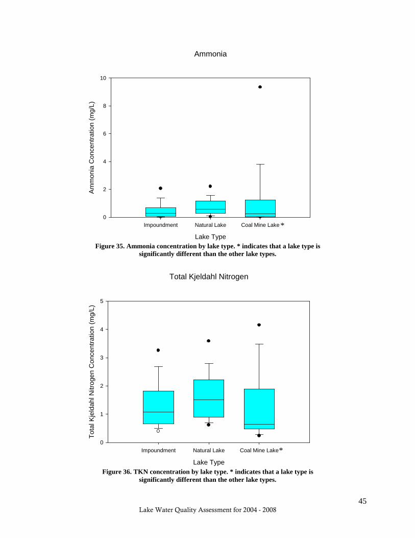
45 Lake Water Quality Assessment for 2004 - 2008
Ammonia
Lake Type
Impoundment Natural Lake Coal Mine Lake
Am
mon
ia C
once
ntra
tion
(mg/
L)
0
2
4
6
8
10
Figure 35. Ammonia concentration by lake type. * indicates that a lake type is
significantly different than the other lake types.
Total Kjeldahl Nitrogen
Lake Type
Impoundment Natural Lake Coal Mine Lake
Tota
l Kje
ldah
l Nitr
ogen
Con
cent
ratio
n (m
g/L)
0
1
2
3
4
5
Figure 36. TKN concentration by lake type. * indicates that a lake type is
significantly different than the other lake types.
*
*

46 Indiana Water Quality Assessment, 2004-2008
Percent of the Water Column that is Oxic
Lake Type
Impoundment Natural Lake Coal Mine Lake
Per
cent
of t
he W
ater
Col
umn
that
is O
xic
(%)
0
20
40
60
80
100
120
Figure 37. Percent of the water column that is oxygenated by lake type. * indicates that a lake type is
significantly different than the other lake types.
pH
Lake Type
Impoundment Natural Lake Coal Mine Lake
pH
7.0
7.5
8.0
8.5
9.0
Figure 38. pH by lake type. * indicates that a lake type is
significantly different than the other lake types.
*
*

47 Lake Water Quality Assessment for 2004 - 2008
Carlson’s Trophic State Index The median trophic state value was obtained for each of the Carlson’s parameters for each lake type.
Secchi Disk TSI. Since Secchi disk TSI was compared between lake types using a Welch’s ANOVA, both the median and mean Secchi disk TSI values for each lake type are reported. Impoundments had the highest median and mean Carlson’s TSI score based on Secchi depth measurement (Figure 39). The median score was 59 and the mean score was 58.5, which are considered to be eutrophic. Natural lakes had a median Secchi disk TSI score of 54 and a mean Secchi disk TSI score of 54.5, which are also considered to be eutrophic. Coal mine lakes had the lowest median and mean Secchi disk TSI scores of 43 and 44.6, respectively, which are mesotrophic scores. After a significant Welch’s ANOVA result was obtained (F = 24.145, p < 0.0005, Table 8), the Games-Howell post hoc test revealed that impoundments were not significantly different from natural lakes (p = 0.119), but coal mine lakes were significantly different from both impoundments (p < 0.005) and natural lakes (p < 0.0005, Table 10). Therefore, as Figure 39 shows, coal mine lakes had a significantly lower Secchi disk TSI than impoundments and natural lakes.
Chlorophyll a TSI. Since Chlorophyll a TSI was compared between lake types using a Welch’s ANOVA, both the median and mean Chlorophyll a TSI values for each lake type are reported. The highest median and mean Carlson’s TSI score based on chlorophyll a concentrations were observed in impoundments (Figure 40), which also had the highest Carlson’s TSI score based on Secchi depth. Impoundments had a median score of 55 and a mean score of 53.9, which are considered eutrophic. Natural lakes had a median Chlorophyll a TSI score of 51 and a mean Chlorophyll a TSI score of 48.9. Both of these scores are considered mesotrophic. Coal mine lakes had the lowest median and mean Chlorophyll a TSI scores of 39 and 41.1, respectively. These scores are also considered mesotrophic. After a significant Welch’s ANOVA result was obtained (F = 12.108, p < 0.0005, Table 8), the Games-Howell post hoc test revealed that impoundments were not significantly different from natural lakes (p = 0.127), but coal mine lakes were significantly different from both impoundments (p < 0.005) and natural lakes (p = 0.001, Table 10). Therefore, as Figure 40 shows, coal mine lakes had a significantly lower chlorophyll a TSI than impoundments and natural lakes.
Total Phosphorus TSI. Impoundments and natural lakes had the same median Carlson’s TSI score based on total phosphorus concentration (Figure 41). The median score in impoundments and natural lakes was 72, indicating hypereutrophic conditions in these lakes. Coal mine lakes had the lowest median score of 42, which is mesotrophic. After a significant Kruskal-Wallis result was obtained (Chi-Square = 65.274, p < 0.0005, Table 8), the sequential Bonferroni procedure revealed that impoundments were not significantly different from natural lakes, but coal mine lakes were significantly different from both impoundments and natural lakes (Table 9). Therefore, as Figure 41 shows, coal mine lakes had a significantly lower total phosphorus TSI than impoundments and natural lakes.

48 Indiana Water Quality Assessment, 2004-2008
Secchi Disk TSI
Lake Type
Impoundment Natural Lake Coal Mine Lake
Secc
hi D
isk
TSI
20
30
40
50
60
70
80
90
Figure 39. Secchi Disk TSI by lake type. * indicates that a lake type is
significantly different than the other lake types.
Chlorophyll a TSI
Lake Type
Impoundment Natural Lake Coal Mine Lake
Chl
orop
hyll
a TS
I
20
30
40
50
60
70
80
90
Figure 40. Chlorophyll a TSI by lake type. * indicates that a lake type is
significantly different than the other lake types.
*
*

49 Lake Water Quality Assessment for 2004 - 2008
Total Phosphorus TSI
Lake Type
Impoundment Natural Lake Coal Mine Lake
Tota
l Pho
spho
rus
TSI
30
40
50
60
70
80
90
100
Figure 41. Total phosphorus TSI by lake type. * indicates that a lake type is
significantly different than the other lake types.
Averaged Score. All of the scores for a given lake were averaged, and the median score for all lake types was obtained (Figure 42). Since the averaged Carlson’s TSI was compared between lake types using a Welch’s ANOVA, both the median and mean averaged Carlson’s TSI values for each lake type are reported. The highest median and mean averaged Carlson’s TSI scores were 60 and 58.9, and were found in impoundments. These scores are considered eutrophic. Natural lakes had a median and mean averaged Carlson’s TSI score of 53 and 53.9, respectively, which are also considered eutrophic. Coal mine lakes had the lowest median and mean averaged Carlson’s TSI of 41 and 42.7, respectively, which are mesotrophic. After a significant Welch’s ANOVA result was obtained (F = 38.491, p < 0.0005, Table 8), the Games-Howell post hoc test revealed that impoundments were significantly different from natural lakes (p = 0.039), and coal mine lakes were significantly different from both impoundments (p < 0.005) and natural lakes (p < 0.0005, Table 10). Therefore, all lakes types were significantly different from one another in terms of averaged Carlson’s TSI score.
*

50 Indiana Water Quality Assessment, 2004-2008
Averaged Carlson's TSI
Lake Type
Impoundment Natural Lake Coal Mine Lake
Car
lson
's T
SI S
core
30
40
50
60
70
80
Figure 42. Averaged Carlson’s TSI by lake type. * indicates that a lake type is
significantly different than the other lake types.
Indiana Trophic State Index Since the Indiana TSI was compared between lake types using a Welch’s ANOVA, both the median and mean Indiana TSI values for each lake type are reported. Natural lakes had median and mean ITSI scores of 27 and 28.5, respectively, which were the highest median and mean scores of all the lake types sampled (Figure 43). Impoundments had a median and mean ITSI score of 24.5 and 25.7, respectively, and coal mine lakes had the lowest median and mean ITSI scores of 13 and 15.7, respectively. In terms of ITSI, after a significant Welch’s ANOVA result was obtained (F = 25.973, p < 0.0005, Table 8), the Games-Howell post hoc test revealed that impoundments were not significantly different from natural lakes (p = 0.433), but coal mine lakes were significantly different from both impoundments (p < 0.005) and natural lakes (p < 0.0005, Table 10). Therefore, as Figure 43 shows, coal mine lakes had a significantly lower ITSI than impoundments and natural lakes.
* * *

51 Lake Water Quality Assessment for 2004 - 2008
Table 9. Results of Sequential Bonferroni procedure for comparison of lake types. MWW = Mann Whitney Wilcoxon, α = 0.05, k = 3. The sequential Bonferroni procedure entails running pairwise comparisons on the different groups (a MWW was chosen because of the non-normal distributions of data) and comparing the p values of these pairwise comparisons to a comparison statistic. If the p value is lower than this statistic, the difference between the groups is significant. If the p value is higher than this statistic, the difference between the groups is not significant.
Parameter Comparison Groups Significance of MWW test
Comparison statistic
Significant Difference?
Maximum Depth (m)
Impoundments vs. Natural Lakes p < 0.0005 α/k = 0.017 Yes Coal Mine Lakes vs. Natural Lakes p = 0.010 α/(k-1) = 0.025 Yes Coal Mine Lakes vs. Impoundments p = 0.014 α/(k-2) = 0.05 Yes
Surface Area (ha)
Coal Mine Lakes vs. Natural Lakes p < 0.0005 α/k = 0.017 Yes Coal Mine Lakes vs. Impoundments p < 0.0005 α/(k-1) = 0.025 Yes Impoundments vs. Natural Lakes p = 0.067 α/(k-2) = 0.05 No
Secchi Depth (m)
Coal Mine Lakes vs. Natural Lakes p < 0.0005 α/k = 0.017 Yes Coal Mine Lakes vs. Impoundments p < 0.0005 α/(k-1) = 0.025 Yes Impoundments vs. Natural Lakes p = 0.042 α/(k-2) = 0.05 Yes
Percent of the water column that is oxic (%)
Coal Mine Lakes vs. Natural Lakes p < 0.0005 α/k = 0.017 Yes Coal Mine Lakes vs. Impoundments p = 0.013 α/(k-1) = 0.025 Yes
Impoundments vs. Natural Lakes p = 0.156 α/(k-2) = 0.05 No Chlorophyll a conc. (mg/m3)
Coal Mine Lakes vs. Impoundments p < 0.0005 α/k = 0.017 Yes Coal Mine Lakes vs. Natural Lakes p = 0.001 α/(k-1) = 0.025 Yes Impoundments vs. Natural Lakes p = 0.051 α/(k-2) = 0.05 No
Nitrate concentration (mg/L)
Coal Mine Lakes vs. Impoundments p = 0.413 α/k = 0.017 No Impoundments vs. Natural Lakes p = 0.416 α/(k-1) = 0.025 No Coal Mine Lakes vs. Natural Lakes p = 0.790 α/(k-2) = 0.05 No
Ammonia concentration (mg/L)
Coal Mine Lakes vs. Natural Lakes p = 0.008 α/k = 0.017 Yes Impoundments vs. Natural Lakes p = 0.011 α/(k-1) = 0.025 Yes Coal Mine Lakes vs. Impoundments p = 0.580 α/(k-2) = 0.05 No
TKN concentration (mg/L)
Coal Mine Lakes vs. Natural Lakes p < 0.0005 α/k = 0.017 Yes Coal Mine Lakes vs. Impoundments p = 0.032 α/(k-1) = 0.025 No Impoundments vs. Natural Lakes p = 0.051 α/(k-2) = 0.05 No
Total phosphorus conc. (mg/L)
Coal Mine Lakes vs. Natural Lakes p < 0.0005 α/k = 0.017 Yes Coal Mine Lakes vs. Impoundments p < 0.0005 α/(k-1) = 0.025 Yes Impoundments vs. Natural Lakes p = 0.631 α/(k-2) = 0.05 No
Total phosphorus TSI
Coal Mine Lakes vs. Natural Lakes p < 0.0005 α/k = 0.017 Yes Coal Mine Lakes vs. Impoundments p < 0.0005 α/(k-1) = 0.025 Yes Impoundments vs. Natural Lakes p = 0.013 α/(k-2) = 0.05 Yes

52 Indiana Water Quality Assessment, 2004-2008
Table 10. Results of Games-Howell post hoc testing for the comparison of lake types.
Parameter Post Hoc Test
Comparison Groups Mean Difference Between Groups (absolute value)
Significance
pH Games-Howell
Impoundments vs. Natural Lakes 0.112 p = 0.223 Coal Mine Lakes vs. Impoundments 0.360 p < 0.0005 Coal Mine Lakes vs. Natural Lakes 0.472 p < 0.0005
Secchi Disk TSI
Games-Howell
Impoundments vs. Natural Lakes 4.026 p = 0.119 Coal Mine Lakes vs. Impoundments 13.881 p < 0.0005 Coal Mine Lakes vs. Natural Lakes 9.855 p < 0.0005
Chlorophyll a TSI
Games-Howell
Impoundments vs. Natural Lakes 4.924 p = 0.127 Coal Mine Lakes vs. Impoundments 12.761 p < 0.0005 Coal Mine Lakes vs. Natural Lakes 7.837 p = 0.001
Averaged Carlson’s TSI
Games-Howell
Impoundments vs. Natural Lakes 5.042 p = 0.039 Coal Mine Lakes vs. Impoundments 16.257 p < 0.0005 Coal Mine Lakes vs. Natural Lakes 11.214 p < 0.0005
Indiana TSI Games-Howell
Impoundments vs. Natural Lakes 2.739 p = 0.433 Coal Mine Lakes vs. Impoundments 9.991 p < 0.0005 Coal Mine Lakes vs. Natural Lakes 12.760 p < 0.0005
Indiana TSI
Lake Type
Impoundment Natural Lake Coal Mine Lake
Indi
ana
TSI S
core
0
10
20
30
40
50
60
Figure 43. Indiana TSI score by lake type. * indicates that a lake type is
significantly different than the other lake types.
*

53 Lake Water Quality Assessment for 2004 - 2008
DISCUSSION
Ecoregion Analysis Secchi Disk Transparency Algae and suspended sediments decrease water clarity in lakes. A deeper Secchi disk reading indicates higher water clarity. Based on Secchi depth, lakes in Ecoregion 72 have higher water clarity than lakes in other ecoregions. Although ITSI scores indicate that the trophic state of lakes in Ecoregion 55 has changed from a eutrophy to a mesotrophy, Ecoregion 55 has the shallowest median Secchi disk reading indicating lower water clarity in Ecoregion 55 than in other ecoregions. Total Phosphorus Phosphorus is often the limiting nutrient in lakes; however, small concentrations of phosphorus can cause eutrophication in lakes. Vollenweider (1975) suggests that 0.10 mg/L or more of total phosphorus in a system can stimulate algal growth, cause reduced oxygen, organism death, and eutrophication (EPA, 2003). Ecoregions 56 and 55 had higher median total phosphorus values than Vollenweider’s suggested upper limit. In the 2004-2008 sampling season, both of these ecoregions had median ITSI scores that indicated a mesotrophic state despite the high total phosphorus median of the lakes. Based on Carlson’s TSI for total phosphorus, both Ecoregions 55 and 56 are considered hypereutrophic. The averaged Carlson’s score for Ecoregions 55 and 56 indicate that the median lakes in these areas are eutrophic. Chlorophyll a Havens and Nürnberg (2004) suggest that with increasing total phosphorus concentrations, chlorophyll a concentrations increase. Using total phosphorus concentration as a predictor for chlorophyll a, Ecoregion 56 should have the highest median concentration of chlorophyll a; however, the highest median concentration of chlorophyll a does not correspond to the highest median concentration of phosphorus as Ecoregion 55 has the second highest median concentration of phosphorus and the highest median concentration of chlorophyll a. The presence of macrophytes (aquatic plants) in a lake can make total phosphorus a poor predictor of chlorophyll a concentration (Rooney and Kalff, 2003). The higher the density of macrophytes in a lake, the lower the concentration of suspended algae (and chlorophyll a) based on total phosphorus concentration, which is especially true during the summer months when the most macrophyte growth occurs in lakes (Rooney and Kalff, 2003) and when our sampling occurred. Nitrogen Nitrogen can enter aquatic systems through fertilizers, wastewater, septic tanks, and atmospheric sources. Due to the atmospheric link, nitrogen is almost never a limiting nutrient in aquatic systems and can contribute, along with phosphorus, to increased productivity in a lake causing eutrophication. Nitrate and ammonia concentrations in water bodies are typically less

54 Indiana Water Quality Assessment, 2004-2008
than 1 mg/L (EPA, 2003). Nitrogenous compounds can become toxic to organisms at concentrations of 10 mg/L or above (EPA, 2003). Excess nitrogen in a system can also contribute to the depletion of oxygen in a system which reduces the percent of the water column that is oxic and causes anoxia (EPA, 2003). The median nitrate and ammonia concentrations for all of the ecoregions were below the 1 mg/L concentration of natural waters indicating that nitrogen is not contributing greatly to eutrophication in these lakes. Percent Water Column Oxic A higher percentage of the water column being oxic indicates that a greater portion of the water column has oxygen that can support biota. The median percentage of oxygenated water in all of the ecoregions was at least 40%. Indiana Trophic State Index In general, Indiana’s lakes have become less productive over time indicating that fewer algal blooms will occur. However, the 2004-2008 sampling period indicated an increase in productivity for lakes within ecoregions 54, 55, and 56. On the other hand, lakes in ecoregions 71 and 72 have become less productive in recent years, possibly indicating that best management practices regarding agriculture and development in watersheds are working in these regions of Indiana. According to ITSI scores, a smaller percentage of lakes sampled between 2004 and 2008 have improved than worsened since the earliest sampling occasion (Figure 29). However, this only represents a change between two sampling periods and provides insufficient information to make assumptions about long-term trends in water quality. Carlson’s Trophic State Index There are many different factors that impact the relationship between Secchi disk transparency measurements, chlorophyll a concentrations, and total phosphorus concentrations. To reduce these variations, the Carlson’s TSI scores from each parameter are averaged. The differing relationships between these parameters are seen in the classification that each parameter gives an ecoregion (Figure 44). This graph represents the category an ecoregion was assigned based on the Carlson’s parameter. A score of 1 indicates oligotrophic, 2 is mesotrophic, 3 is eutrophic, and 4 is hypereutrophic. From Figure 44, it can be seen that the Secchi disk transparency parameter gives the most accurate representation of the averaged Carlson’s TSI score.

55 Lake Water Quality Assessment for 2004 - 2008
0
1
2
3
4
54 55 56 71 72
Cate
gory
Ecoregion
Carlson's TSI Comparison
Secchi Disk
Chlorophyll a
Total Phosphorus
Averaged Score
Figure 44. Median Carlson’s TSI for lakes within the Indiana ecoregions.
1 = oligotrophic; 2 = mesotrophic; 3 = eutrophic; 4 = hypereutrophic
Comparison of ITSI and Carlson’s TSI The ITSI designates 21 more lakes as being oligotrophic than the Carlson’s TSI indicates. The ITSI designates 12 fewer lakes as being mesotrophic than does the Carlson’s TSI and 12 fewer lakes as eutrophic than does the Carlson’s TSI. The ITSI also designates 19 fewer lakes as being hypereutrophic than does the Carlson’s TSI. Therefore, the ITSI gives a more positive outlook on Indiana’s lakes than does the Carlson’s TSI. Basin Analysis At the α = 0.05 level, hypolimnetic SRP and ammonia showed significant differences (Table 4) between the two samples (site one and sites two and three combined). These significant differences may be due to differences in depth between the sampling sites. Indeed, hypolimnetic SRP and ammonia concentrations are influenced by depth in many ways.
Specifically, deep lakes are more likely to undergo thermal stratification than shallow lakes. In addition, the isolation of hypolimnetic waters that occurs during thermal stratification can lead to a depletion of dissolved oxygen in the hypolimnion (Figure 45). Indeed, hypolimnetic decomposition often consumes dissolved oxygen faster than it can be replaced by the overlying waters, and the hypolimnion is often too dark for algae to produce more oxygen through photosynthesis. This depletion of oxygen in deeper waters in turn affects nutrient cycling. For example, under aerobic conditions, SRP in the form of phosphate (PO4
3-) binds to ferric iron (Fe3+) in lake sediments, forming insoluble complexes (Gatcher et al., 1988). However, when the

56 Indiana Water Quality Assessment, 2004-2008
hypolimnetic concentration of dissolved oxygen decreases in a lake (often associated with thermal stratification), the sediment redox potential also decreases, and the ferric iron complexes dissolve (Gatcher et al., 1988). Thus, iron and phosphates (SRP) are released back into the hypolimnion in low-oxygen conditions. In addition, the concentration of dissolved oxygen in hypolimnetic waters and sediments determines the predominant type of decomposition that takes place (aerobic or anaerobic). If dissolved oxygen concentrations are low, anaerobic decomposition dominates, and ammonia is released as a byproduct into the hypolimnion.
Figure 45. Dissolved oxygen profile showing hypolimnetic anoxia.
Lake depth may also affect pH, which in turn affects nutrient concentrations. For
example, in shallow lakes, algal photosynthesis may deplete carbon dioxide (CO2) in the water column and subsequently increase the pH of the water. At pH values above 9.5, SRP can be released from the sediments at rates similar to those under anoxic conditions (Holdren et al., 2001).
Our data did show a significantly different relationship between depth and hypolimnetic ammonia and SRP concentration (Regression: F = 0.415, p = 0.520, R2 = 0.003 for ammonia and F = 0.108, p = 0.743, R2 = 0.001 for SRP), see Table 11 and Figures 46 and 47. However, this was likely due to the large number of data at the detection limit for these parameters. In addition, a statistically significant difference in the concentration of hypolimnetic ammonia and SRP between sampling sites may be due to a difference in depth between these sites. Indeed, for the multi-basin lakes that were sampled in 2006 and 2008, depth was significantly different between site one and the combined sites two and three (paired t test: t = 2.717, p = 0.009). Also, if depth was in fact responsible for the differences in hypolimnetic ammonia and SRP between sites one and the combined sites two and three, one would expect deeper sites to have a higher concentration of hypolimnetic ammonia and SRP than shallower sites (as explained above). This was indeed demonstrated by our data, since site one (the deepest sampling site) had a
0
2
4
6
8
10
12
14
0 2 4 6 8 10
Dept
h (m
)
Dissolved Oxygen (ppm)
Dissolved Oxygen Profile of a Thermally Stratified Lake
57 Lake Water Quality Assessment for 2004 - 2008
significantly higher concentration of hypolimnetic ammonia and SRP than the shallower sites two and three (Table 4).
Chlorophyll a concentration and Carlson’s TSI were significantly different between the two samples at the α = 0.1 level (Table 4). These parameters are also influenced by lake depth. For example, shallow lakes tend to be more productive than deeper lakes. This is because in shallow lakes, a higher percentage of the water volume is in the photic zone than in deep lakes. Thus algal photosynthesis can occur in a larger portion of the water column in shallow lakes than in deep lakes (Holdren et al., 2001). In addition, shallow lakes may not stratify since the entire water column is more easily mixed by wind and wave action than in deep lakes. Thus, nutrients from the sediments are more readily available to the entire water column in shallow lakes than in deep lakes. Nutrients from the sediments, combined with sunlight from the surface, fuel algal growth in shallow lakes. All these factors should result in higher chlorophyll a concentrations in shallow lakes than in deep lakes.
Indeed, our data showed a significant negative relationship between chlorophyll a
concentration and depth (Table 11 and Figure 48; Regression: F = 17.081, p < 0.0005, R2 = 0.105). An R2 value of 0.105 indicates that depth only explained 10.5% of the variation in chlorophyll a concentration. This was not surprising since many other factors, such as phosphorus concentration and the availability of sunlight can influence chlorophyll a concentrations. Furthermore, the small p value indicates that the slope of the line relating depth to chlorophyll a concentration was not zero. Therefore, a statistically significant relationship existed between depth and chlorophyll a concentration. Additionally, since Carlson’s TSI is based on Secchi disk transparency, total phosphorus, and chlorophyll a, any relationship between chlorophyll a and depth implies a relationship between Carlson’s TSI and depth.
If depth was responsible for the differences in chlorophyll a concentration and Carlson’s
TSI between sites one and the combined sites two and three, one would expect deeper sites to have lower chlorophyll a concentrations and Carlson’s TSI scores than shallower sites. Indeed, our data indicated that site one (the deepest sampling site) had a significantly lower chlorophyll a concentration and Carlson’s TSI score than the shallower sites two and three (Table 4). Therefore, the statistically significant difference in chlorophyll a concentration between sampling sites may also be due to the difference in depth between these sites. Table 11. Regression results for the basin analysis.
Independent variable
Dependent Variable Test R2 Test Statistic
Significance
Depth (m) Hypolimnetic ammonia concentration (mg/L)
Linear Regression
0.003 F = 0.415 p = 0.520
Depth (m) Hypolimnetic SRP concentration (mg/L)
Linear Regression
0.001 F = 0.108 p = 0.743
Depth (m) Chlorophyll a concentration (mg/m3)
Linear Regression
0.105 F = 17.081 p < 0.0005

58 Indiana Water Quality Assessment, 2004-2008
0
5
10
15
20
25
30
35
40
0 0.5 1 1.5 2 2.5 3 3.5 4 4.5 5
Dep
th (m
)
Ammonia concentration (mg/L)
Depth vs. Hypolimnetic Ammonia
Figure 46. The relationship between depth and hypolimnetic ammonia in Indiana’s multi-basin lakes.
0
5
10
15
20
25
30
35
40
0 0.1 0.2 0.3 0.4 0.5
Dept
h (m
)
SRP concentration (mg/L)
Depth vs. Hypolimnetic Soluble Reactive Phosphorus
Figure 47. The relationship between depth and hypolimnetic SRP in Indiana’s multi-basin lakes.

59 Lake Water Quality Assessment for 2004 - 2008
0
5
10
15
20
25
30
35
40
0 20 40 60 80 100 120 140
Dep
th (m
)
Chlorophyll a concentration (mg/m3)
Depth vs. Chlorophyll a
Figure 48. The relationship between depth and chlorophyll a concentration in Indiana’s multi-basin lakes.
Water quality analysis through time Because lakes are dynamic systems and constantly receive inputs from their surrounding watersheds, it is to be expected that water quality parameters will change over time. Indeed, our data showed that for the lakes sampled between 2004 and 2008, several water quality parameters were significantly different in 2004-2008 from the values recorded in the earliest sampling records of these same lakes. The direction and magnitude of the changes in water quality convey valuable information.
For example, the fact that the earliest sampling record had a significantly higher Secchi
depth, light transmission at three feet, one percent light level, and percent of the water column that is oxic, and a significantly lower chlorophyll a concentration, than the most recent sampling record for all lakes sampled between 2004 and 2008 may indicate a decline in the water quality of these lakes over time. However, some statistically significant differences in parameters over time were not large in enough to draw such conclusions about long-term trends. For example, Secchi depth was only 0.085 meters higher, one percent light level was only 2.25% higher, and chlorophyll a concentration was only 2.49 mg/m3 lower, for the earliest sampling record than for the most recent sampling record for lakes sampled between 2004 and 2008 (Table 5). These differences may fall within reasonable ranges of seasonal variation. In addition, the earliest sampling record had significantly higher nitrate, ammonia, TKN, SRP, and plankton than the most recent sampling record for all lakes sampled between 2004 and 2008 (Table 5). This could indicate an improvement in the water quality of these lakes over time, and could provide evidence that best management practices regarding agriculture and development in watersheds are working in Indiana.

60 Indiana Water Quality Assessment, 2004-2008
Comparison of Lake Types Morphometry Coal mine lakes had significantly smaller surface areas than both impoundments and natural lakes, whereas there was no significant difference in surface area between impoundments and natural lakes. Therefore, our data revealed that surface area contributed to the uniqueness of coal mine lakes. This was to be expected, since coal mine lakes were formed from strip mining pits, rather than the damming of rivers or the natural process of glacial retreat, which tend to create lakes with greater surface areas. As Figure 30 shows, natural lakes had the highest maximum depth, impoundments had the lowest maximum depth, and coal mine lakes had an intermediate maximum depth. This was to be expected since the majority of Indiana’s natural lakes are kettle lakes (see earlier section on Lake Classification), which tend to be very deep, and strip mines tend to be deeper than reservoirs. However, at the α = 0.05 level, all lake types were significantly different from one another regarding maximum depth (Table 9). Secchi Disk Transparency As shown in Figure 31, coal mine lakes had the deepest median Secchi disk transparency of all the lake types sampled. This could be due to lower nutrient concentrations (and therefore fewer algae) in coal mine lakes than in other lake types (see below). In addition, coal mine lakes, because of their smaller surface areas (see above), may be less affected than impoundments and natural lakes by turbidity from wind and wave action. However, at the α = 0.05 level, all lake types were significantly different from one another regarding Secchi disk transparency (Table 9). Total Phosphorus Coal mine lakes had significantly lower total phosphorus concentrations than both impoundments and natural lakes, whereas there was no significant difference in total phosphorus concentration between impoundments and natural lakes. Therefore, our data revealed that total phosphorus concentration contributed to the uniqueness of coal mine lakes. The lower concentration of total phosphorus in coal mine lakes than in impoundments and natural lakes may be due to the fact that coal mine lakes have smaller watersheds than other lake types. Indeed, the watersheds of many coal mine lakes are defined by the overburden ridges formed during the mining process. A smaller watershed could in turn lead to a smaller volume of runoff and fewer nutrient additions from the surrounding land. In addition, the oldest surface mine in the Greene-Sullivan State Forest and Minnehaha Fish and Wildlife Area was abandoned in 1918 (GIS data); therefore, lakes that formed in these coal mining strip pits may be relatively nutrient-poor because they are young (by geological standards). As explained earlier, the natural processes of eutrophication occur over thousands of years. Chlorophyll a Coal mine lakes had significantly lower chlorophyll a concentrations than both impoundments and natural lakes, whereas there was no significant difference in chlorophyll a concentration between impoundments and natural lakes. Therefore, our data revealed that

61 Lake Water Quality Assessment for 2004 - 2008
chlorophyll a concentration contributed to the uniqueness of coal mine lakes. The lower concentration of chlorophyll a in coal mine lakes than in impoundments and natural lakes may have been due to the fact that coal mine lakes had lower concentrations of limiting nutrients for algal growth (such as phosphorus) than other lake types (see above). Coal mine lakes also had lower concentrations of ammonia and TKN than other lake types; however nitrate concentrations were not significantly lower in coal mine lakes than in impoundments or natural lakes (see below). Algal growth in coal mine lakes might also have been limited by a number of other factors such as excessive predation by zooplankton or the effects of pH (see below). Finally, algal growth in the coal mine lakes might also have been affected by some unknown limiting factor or toxicant introduced by the mining process. Nitrate There was no statistically significant difference in nitrate concentration between the three different lake types. Therefore, nitrate concentration did not contribute to the uniqueness of coal mine lakes. However, as Figure 34 shows, coal mine lakes had the smallest range of nitrate concentrations of all the lake types that were sampled. In addition, other types of nitrogen such as ammonia and TKN were significantly lower in coal mine lakes than in impoundments and natural lakes (see below). Ammonia Coal mine lakes had significantly lower ammonia concentrations than both impoundments and natural lakes, whereas there was no significant difference in ammonia concentration between impoundments and natural lakes. Therefore, our data revealed that ammonia concentration contributed to the uniqueness of coal mine lakes. Like phosphorus concentration, ammonia concentration may have been lower in coal mine lakes than in other lake types because coal mine lakes have small watersheds compared to other lake types. Specifically, the smaller watersheds of coal mine lakes are less likely to receive runoff that is contaminated with nitrogen-rich agricultural fertilizers. In addition, the watersheds of coal mine lakes are largely undeveloped; therefore, unlike impoundments and natural lakes, coal mine lakes do not receive nitrogen and phosphorus inputs from septic tanks and lawn fertilizers. Finally, as explained earlier, the lower concentration of nutrients such as phosphorus, ammonia, and TKN in coal mine lakes than in other lake types may be due to the fact that coal mine lakes are relatively young systems. Total Kjeldahl Nitrogen Coal mine lakes had significantly lower TKN concentrations than both impoundments and natural lakes, whereas there was no significant difference in TKN concentration between impoundments and natural lakes. Therefore, our data revealed that TKN concentration contributed to the uniqueness of coal mine lakes. As explained above, a lower concentration of TKN in coal mine lakes than in impoundments and natural lakes may be due to the fact that coal mine lakes have smaller and less developed watersheds than impoundments and natural lakes, and are relatively young compared to other lake types, especially natural lakes.

62 Indiana Water Quality Assessment, 2004-2008
Percent Water Column Oxic Coal mine lakes had a significantly higher percent of the water column that was oxygenated than both impoundments and natural lakes, whereas there was no significant difference in percent of the water column oxic between impoundments and natural lakes. Therefore, our data revealed that percent of the water column oxic contributed to the uniqueness of coal mine lakes. Coal mine lakes may have had a higher percentage of the water column that was oxygenated because of their relatively low nutrient and chlorophyll a concentrations with respect to impoundments and natural lakes. Specifically, lower nutrients and algal growth in coal mine lakes could have potentially translated to lower a biological oxygen demand (BOD) than in impoundments and natural lakes. BOD is a measure of the oxygen used by microorganisms to decompose organic material. Lakes with lower nutrient concentrations and algal growth typically have lower productivity and smaller volumes of dead organic material (such as algae and plants) than lakes with higher nutrient concentrations and algal growth. A smaller volume of dead organic material would then imply a lower BOD, and a higher percent of the water column that is oxygenated. pH Coal mine lakes had a significantly lower pH than both impoundments and natural lakes, whereas there was no significant difference in pH between impoundments and natural lakes. Therefore, our data revealed that pH contributed to the uniqueness of coal mine lakes. Coal mine lakes are susceptible to the effects of acid mine drainage, which occurs when iron-sulfur compounds in mine waste are exposed to air and moisture and are oxidized by chemical and microbial reactions to sulfuric acid (Gyure et al., 1987). Acidic leachates then flow through soil and mine spoils, and eventually into coal mine lakes, picking up dissolved materials on their way.
Low water pH caused by acid mine drainage can have negative implications for
productivity. Specifically, low pH can increase the solubility (and thus aqueous concentration) of copper, aluminum, and other metals such as lead and arsenic in lakes. High concentrations of copper have been shown to inhibit algal growth (Lehman et al., 2004) and high concentrations of aluminum can decimate fish populations by precipitating on fish gills, thus impairing gaseous exchange. Reservoir 29, one of the coal mine lakes in the Greene-Sullivan State Forest has historically been affected by acid mine drainage, and had an epilimnetic pH of 2.7 in 1987 (Gyure et al., 1987). Management efforts such as liming helped increase Reservoir 29’s epilimnetic and hypolimnetic pH to 6.9 and 6.1, respectively, by August, 2008; however, Reservoir 29’s pH remains below the average for all the coal mine lakes that were sampled in 2008.
Carlson’s Trophic State Index
Secchi Disk TSI. Coal mine lakes had a significantly lower Secchi disk TSI than both impoundments and natural lakes, whereas there was no significant difference in Secchi disk TSI between impoundments and natural lakes. Therefore, our data revealed that Secchi Disk TSI contributed to the uniqueness of coal mine lakes. Because Secchi disk TSI is based on Secchi disk transparency, and since coal mine lakes had the lowest Secchi disk transparency of all the

63 Lake Water Quality Assessment for 2004 - 2008
lakes types sampled between 2004 and 2008, it was to be expected that coal mine lakes would also have lower Secchi disk TSI values than impoundments and natural lakes.
Chlorophyll a TSI. Coal mine lakes had a significantly lower chlorophyll a TSI than both impoundments and natural lakes, whereas there was no significant difference in chlorophyll a TSI between impoundments and natural lakes. Therefore, our data revealed that chlorophyll a TSI contributed to the uniqueness of coal mine lakes. Again, since chlorophyll a TSI is based on chlorophyll a concentration, and since coal mine lakes had a significantly lower chlorophyll a concentration than both impoundments and natural lakes, it was to be expected that coal mine lakes would have a significantly lower chlorophyll a TSI than the other lake types.
Total Phosphorus TSI. There was no significant difference in total phosphorus TSI between impoundments, natural lakes, and coal mine lakes. This is surprising, given that total phosphorus TSI is based on total phosphorus concentration, and that coal mine lakes had a significantly lower total phosphorus concentration than the other lake types sampled. However, even though there was no statistically significant difference in total phosphorus TSI between the three lake types, coal mine lakes still had the lowest total phosphorus TSI of all the lake types.
Averaged Score. There was no significant difference in averaged Carlson’s TSI score between impoundments, natural lakes, and coal mine lakes. This was probably due to the fact that the averaged Carlson’s TSI score is based on Secchi disk TSI, chlorophyll a TSI, and total phosphorus TSI, and to the lack of significant differences in total phosphorus TSI scores between lake types. Even though there was no significant difference in averaged Carlson’s TSI score between lake types, coal mine lakes still had the lowest averaged Carlson’s TSI, which indicates that between 2004 and 2008, coal mine lakes were less productive than impoundments and natural lakes. Reasons for depressed productivity in coal mine lakes (as compared to other lake types) were discussed above, and include possible nutrient limitation, sunlight limitation, or the effects of other factors such as pH (from acid mine drainage) or unknown toxicants.
Indiana Trophic State Index. Coal mine lakes had a significantly lower ITSI than both impoundments and natural lakes, whereas there was no significant difference in ITSI between impoundments and natural lakes. Therefore, our data revealed that ITSI contributed to the uniqueness of coal mine lakes. Since the ITSI is comprised of ten nutrient and water quality metrics (see the section on Lake Classification), the fact that coal mine lakes had a significantly lower ITSI than impoundments and natural lakes further implies that between 2004 and 2008, coal mine lakes were less productive than the other sampled lake types.
CONCLUSIONS
In this report, we’ve analyzed lake assessment data collected through the Indiana Clean Lakes Program during the period of 2004 through 2008. This data set represents four summers of sampling since staff were doing fieldwork for the National Lakes Assessment during 2007. These data were examined for long-term trends, for regional differences, for differences in lake type, and for differences in sampling location.

64 Indiana Water Quality Assessment, 2004-2008
When results for the present study (2004 – 2008) were compared with the earliest CLP data collected from the same lakes, we discovered that 54 percent of the lakes had an increase in trophic state, as determined by the Indiana Trophic State Index, 43 percent had a decrease in trophic state, and 3 percent had no significant change. The parameters that showed statistically significant changes to account for the overall worsening in trophic state between these lake populations included: lower Secchi disk transparency, lower light transmission, higher dissolved oxygen saturation, lower percent water column oxygenated, higher mean nitrate concentration, higher mean ammonia concentration, and higher chlorophyll a concentration. Total phosphorus was lower slightly and SRP was significantly lower. The mean Indiana TSI scores for all lakes sampled during the current study were 1.4 points lower but this was not a significant change. So overall, there was a slight improvement in mean Indiana TSI score but more lakes had increases and fewer lakes had decreases in the TSI. Lakes located in southern Indiana (Ecoregions 71 and 72) had lower mean Indiana TSI scores than lakes in northern Indiana and this mean decreased between earlier samples and the 2004-2008 sampling period. In contrast, lakes in northern and central Indiana (Ecoregions 54, 55, and 56) had higher mean Indiana TSI scores and the mean scores for lakes in these ecoregions increased in the most recent sampling. Our analysis of sampling location showed that sampling at one location over the deepest water is representative of most conditions in lakes with complex basins. The only parameters that were significantly different between the deep-water site and shallower basins at the α = 0.05 level were hypolimnetic SRP and hypolimnetic ammonia. Both of these parameters are influenced by redox changes due to anoxia in productive lakes. Chlorophyll a was lower at the deep water sites at the α = 0.1 level. The three primary lake types in Indiana, based on origin, are natural, impoundments, and coal mine lakes. Natural lakes are deepest and have intermediate Secchi disk transparency. Impoundments are the most shallow and have the worst Secchi disk transparency. Coal mine lakes have intermediate depth and the highest Secchi disk transparency. For most other parameters, the natural lakes and impoundments are similar. The coal mine lakes, because of their origin, are significantly different from the other two lake types in a number of areas. Coal mine lakes have lower phosphorus, chlorophyll, ammonia, TKN, pH, and Indiana TSI scores, and higher oxygenation than the natural lakes and impoundments.

65 Lake Water Quality Assessment for 2004 - 2008
REFERENCES APHA et al. 1998. Standard Methods for the Examination of Water and Wastewater,
20th edition. American Public Health Association, Washington, D.C. Carlson, R.E. 1977. A trophic state index for lakes. Limnology and Oceanography, 2(2):361-
369. Clark, G.A, ed. 1980. The Indiana Water Resource – Availability, Uses, and Needs. Governor’s
Water Resource Study Commission, State of Indiana, Indianapolis. Cooke, G.D. et al. 1993. Management of Lakes and Reservoirs, Second Edition. Lewis
Publishers, Ann Arbor, Michigan. EPA. 2004. Environmental Protection Agency. EPA’s Clean Lakes Program.
http://www.epa.gov/owow/lakes/cllkspgm.html (1/28/2009). EPA. 2003. Environmental Protection Agency. Monitoring and Assessing Water Quality.
http://www.epa.gov/volunteer/stream/index.html (1/28/2009). Freshwater Foundation. 1985. A Citizen’s Guide to Lake Protection. Minnesota Pollution
Control Agency, Minneapolis. Gatcher, R., J.S. Meyer, and A. Mares. 1988. Contribution of bacteria to release and fixation of phosphorus in lake sediments. American Society of Limnology and Oceanography. 33(6): 1542-1550. Gyure, R.A., A. Konopka, A. Brooks, and W. Doemel. 1987. Algal and Bacterial Activities in
Acidic (pH 3) Strip Mine Lakes. Applied and Environmental Microbiology. 53(9): 2069-2076.
Havens, K. and G. Nürnberg. 2004. The Phosphorus-Chlorophyll Relationship in Lakes:
Potential Influences of Color and Mixing Regime. Lake and Reservoir Management. 20(3):188-196.
Holdren, C., W. Jones, and J. Taggart. 2001. Managing Lakes and Reservoirs. N. Am. Lake
Manage. Soc. and Terrene Inst. in coop. with Off. Water Assess. Watershed Prot. Div. U.S. Environ. Prot. Agency, Madison, WI.
Hutchinson, G.E. 1957. A Treatise on Limnology. Volume I: Geography, Physics, and
Chemistry. John Wiley and Sons, Inc., New York. Hutchinson, G.E. and H. Loeffler. 1956. The thermal classification of lakes. Proc. Nat. Acad.
Sci., 42:84-86. IDNR. 1993. Indiana Lakes Guide. Department of Natural Resources, Indianapolis.

66 Indiana Water Quality Assessment, 2004-2008
Jones, W. 1996. Indiana lake Water Quality Update for 1989-1993. Indiana Department of Environmental Management Clean Lakes Program, Indianapolis, Indiana.
Kelly, L. 1971. Soil Survey of Sullivan County, Indiana. United States Department of
Agriculture, Soil Conservation Service, in cooperation with the Purdue University Agricultural Experiment Station: 2-73. http://soils.usda.gov/survey/online_surveys/indiana/sullivan/sullivan.pdf (1/28/2009).
Lehman, J.T., A. Bazzi, T. Nosher, and J.O. Nriagu. 2004. Copper inhibition of phytoplankton in
Saginaw Bay, Lake Huron. Canadian Journal of Fisheries and Aquatic Sciences. 61: 1871–1880.
McCarter, P. 1988. Soil Survey of Greene County, Indiana. United States Department of
Agriculture, Soil Conservation Service, in cooperation with Purdue University Agricultural Experiment Station and Indiana Department of Natural Resources, Soil and Water Conservation Committee: 1-226. http://soildatamart.nrcs.usda.gov/manuscripts/IN055/0/greene.pdf (1/28/2009).
Olem, H. and G. Flock, eds. 1990. Lake and Reservoir Restoration Guidance Manual, 2nd
Edition. EPA 440/4-90-006. Prep. By N. Am. Lake Manage. Soc. For U.S. EPA, Washington, D.C.
Omernik, J.M. and A.L. Gallant. 1988. Ecoregions of the Upper Midwest. EPA/600/3-88/037.
U.S. Environmental Protection Agency, Environmental Research laboratory, Corvallis, Oregon.
Prescott, G.W. 1982. Algae of the Western Great Lakes Area. Otto Koeltz Science Publishers,
West Germany. Rooney, N. and J. Kalff. 2003. Submerged Macrophyte-bed Effects on Water-Column
Phosphorus, Chlorophyll a, and Bacterial Production. Ecosystems. 6:797-807 Thompson, T.A. 1998. Bedrock Geology of Indiana. Indiana Geological Survey.
http://igs.indiana.edu/geology/structure/bedrockgeology/index.cfm (2/11/2009). Ward, H.B. and G.C. Whipple. 1959. Freshwater Biology, Second Edition. W.T.
Edmondson, editor. John Wiley & Sons, Inc., New York. Wehr, J.D. and R.G. Sheath. 2003. Freshwater ALgae of North America, Ecology and Classification. Academic Press, San Diego. Whitford, L.A. and G.J. Schumacher. 1984. A Manual of Fresh-Water Algae.
Sparks Press, Raleigh, N.C.
GIS Data
67 Lake Water Quality Assessment for 2004 - 2008
All shapefiles were obtained from the Indiana Geographic Information Council’s IndianaMap. Available online at http://129.79.145.7/arcims/statewide_mxd/download.html (last accessed 3/3/2009). BEDROCK_GEOL_MM48_IN. 1987. 1:500,000-scale polygon shapefile depicting systems and
selected groups, formations, and other stratigraphic units. Generalized lithologic characterizations are also provided. Digitized from the following published paper map: Indiana Geological Survey Miscellaneous Map 48.
HIGHWAYS_INDOTMODEL_IN. 2004. 1:24,000-scale line shapefile depicting Interstate, U.S., and State Highways. Attributes include route numbers and the number of lanes. Obtained from the Indiana Department of Transportation. The highways that are shown are a subset of the Indiana Statewide Travel Demand Model (version 4) and duplicate general traffic patterns, so that detailed networks at interchanges and ramps are not represented.
HYDROGRAPHY_POLY_NHD_IN. 2000. 1:100,000-scale polygon shapefile depicting
Indiana’s canals, lakes, large streams, and swamps or marshes. Derived from the National Hydrography Dataset (NHD).
LANDSURVEY_COUNTY_POLY_IN. 1:24,000-scale polygon shapefile depicting Indiana’s
County boundaries. Projection: Universal Transverse Mercator (UTM)North American Datum (NAD) 1983 zone 16.
NATURAL_REGIONS_IDNR_IN. 1984. 1:800,000-scale polygon shapefile depicting DNR
natural regions and their subsections. Obtained from the Indiana Department of Natural Resources, Division of Nature Preserves, Indiana Natural Heritage Data Center.
SOILS_STATSGO_IN. 1994. 1:250,000-scale polygon shapefile showing generalized soil
associations. Derived from the State Soil Geographic (STATSGO) data base, which is a digital general soil association map developed by the National Cooperative Soil Survey, U.S. Department of Agriculture. The soil maps for STATSGO are compiled by generalizing more detailed soil survey maps.