indexing methods for moving object databases: games and other

Appeared in the Proceedings of the ACM SIGMOD Conference, pp. 169–180, New York, June 2013

Indexing Methods for Moving Object Databases: Gamesand Other Applications∗

Hanan Samet§

Jagan Sankaranarayanan‡†

Michael Auerbach§

§University of Maryland, College Park, MD

‡NEC Labs America, Cupertino, CA

[email protected], [email protected], [email protected]

ABSTRACTMoving object databases arise in numerous applications such astraffic monitoring, crowd tracking, and games. They all requirekeeping track of objects that move and thus the database of objectsmust be constantly updated. The cover fieldtree (more commonlyknown as the loose quadtree and the loose octree, depending onthe dimension of the underlying space) is designed to overcome thedrawback of spatial data structures that associate objects with theirminimum enclosing quadtree (octree) cells which is that the size ofthese cells depends more on the position of the objects and less ontheir size. In fact, the size of these cells may be as large as the entirespace from which the objects are drawn. The loose quadtree (oc-tree) overcomes this drawback by expanding the size of the spacethat is spanned by each quadtree (octree) cell c of width w by a cellexpansion factor p (p > 0) so that the expanded cell is of width(1 + p) ·w and an object is associated with its minimum enclosingexpanded quadtree (octree) cell. It is shown that for an object owith minimum bounding hypercube box b of radius r (i.e., half thelength of a side of the hypercube), the maximum possible width wof the minimum enclosing expanded quadtree cell c is just a func-tion of r and p, and is independent of the position of o. Normalizingw via division by 2r enables calculating the range of possible ex-panded quadtree cell sizes as a function of p. For p ≥ 0.5 the rangeconsists of just two values and usually just one value for p ≥ 1.

∗This work was supported in part by the National Science Founda-tion under grants CCF-05-15241, IIS-0713501, IIS-10-18475, IIS-12-19023, Microsoft Research, Google, NVIDIA, the E.T.S. Wal-ton Visitor Award of the Science Foundation of Ireland, and theNational Center for Geocomputation at the National University ofIreland at Maynooth.†Work done while the author was at the University of Maryland.

Permission to make digital or hard copies of all or part of this work forpersonal or classroom use is granted without fee provided that copies arenot made or distributed for profit or commercial advantage and that copiesbear this notice and the full citation on the first page. To copy otherwise, torepublish, to post on servers or to redistribute to lists, requires prior specificpermission and/or a fee.SIGMOD’13, June 22–27, 2013, New York, New York, USA.Copyright 2013 ACM 978-1-4503-2037-5/13/06 ...$15.00.

This makes updating very simple and fast as for p ≥ 0.5, thereare at most two possible new cells associated with the moved ob-ject and thus the update can be done in O(1) time. Experimentswith random data showed that the update time to support motionin such an environment is minimized when p is infinitesimally lessthan 1, with as much as a one order of magnitude increase in thenumber of updates that can be handled vis-a-vis the p = 0 case in agiven unit of time. Similar results for updates were obtained for anN-body simulation where improved query performance and scal-ability were also observed. Finally, in order amplify the paper, avideo titled “Crates and Barrels” was produced which is an N-bodysimulation of 14,000 objects. The video as well as a JAVA appletthat illustrates the behavior of the loose quadtree are both availablefrom http://www.cs.umd.edu/~hjs/loosequad/.

Categories and Subject DescriptorsE.1 [Data]: Data Structures

General TermsAlgorithm, Performance

Keywordsgame databases, moving objects, spatial data structures, coverfieldtree, loose quadtree, loose octree, spatial indexing, spatialdatabases, game programming

1. INTRODUCTIONOne of the motivations for the development of geographic infor-

mation systems (GIS) is to keep track of objects (e.g., QUILT [38,41], and the SAND Browser [11, 36]) for both location-based andfeature-based queries [4]. Similar needs arise in game applications(e.g., [9,16]), where the difference is that the objects are not usuallystatic. Instead, they are constantly moving and thus the database ofobjects must be constantly updated. An attractive method of repre-senting spatial objects to support the tracking process uses an objecthierarchy where minimum bounding hypercube boxes (e.g., an R-tree [15,37]) are used to speed up the process of detecting if objectsare present or overlap other objects. One of the drawbacks of sucha representation is that the hierarchies of different sets of objects

http://www.cs.umd.edu/~hjs/loosequad/


are not in registration thereby making set operations between thetwo sets such as unions and intersections more complex.

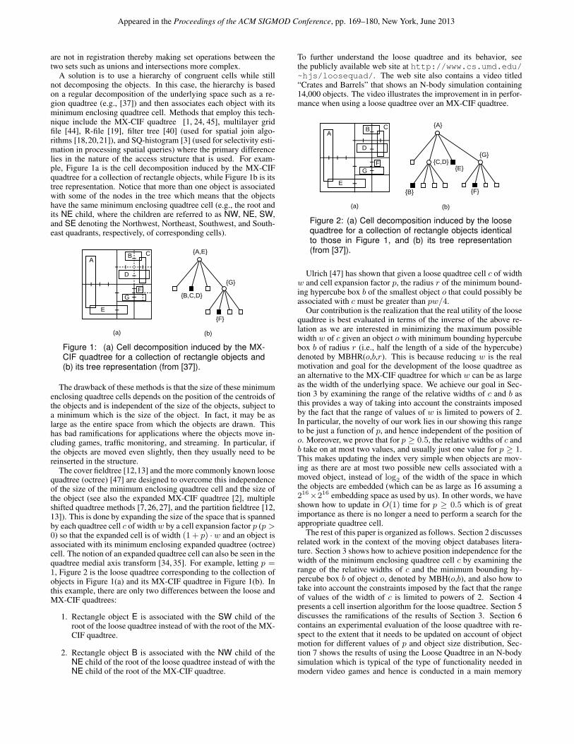
A solution is to use a hierarchy of congruent cells while stillnot decomposing the objects. In this case, the hierarchy is basedon a regular decomposition of the underlying space such as a re-gion quadtree (e.g., [37]) and then associates each object with itsminimum enclosing quadtree cell. Methods that employ this tech-nique include the MX-CIF quadtree [1, 24, 45], multilayer gridfile [44], R-file [19], filter tree [40] (used for spatial join algo-rithms [18,20,21]), and SQ-histogram [3] (used for selectivity esti-mation in processing spatial queries) where the primary differencelies in the nature of the access structure that is used. For exam-ple, Figure 1a is the cell decomposition induced by the MX-CIFquadtree for a collection of rectangle objects, while Figure 1b is itstree representation. Notice that more than one object is associatedwith some of the nodes in the tree which means that the objectshave the same minimum enclosing quadtree cell (e.g., the root andits NE child, where the children are referred to as NW, NE, SW,and SE denoting the Northwest, Northeast, Southwest, and South-east quadrants, respectively, of corresponding cells).

(a) (b)

A

E

GF

D

CB

{F}

{G}

{A,E}

{B,C,D}

Figure 1: (a) Cell decomposition induced by the MX-CIF quadtree for a collection of rectangle objects and(b) its tree representation (from [37]).

The drawback of these methods is that the size of these minimumenclosing quadtree cells depends on the position of the centroids ofthe objects and is independent of the size of the objects, subject toa minimum which is the size of the object. In fact, it may be aslarge as the entire space from which the objects are drawn. Thishas bad ramifications for applications where the objects move in-cluding games, traffic monitoring, and streaming. In particular, ifthe objects are moved even slightly, then they usually need to bereinserted in the structure.

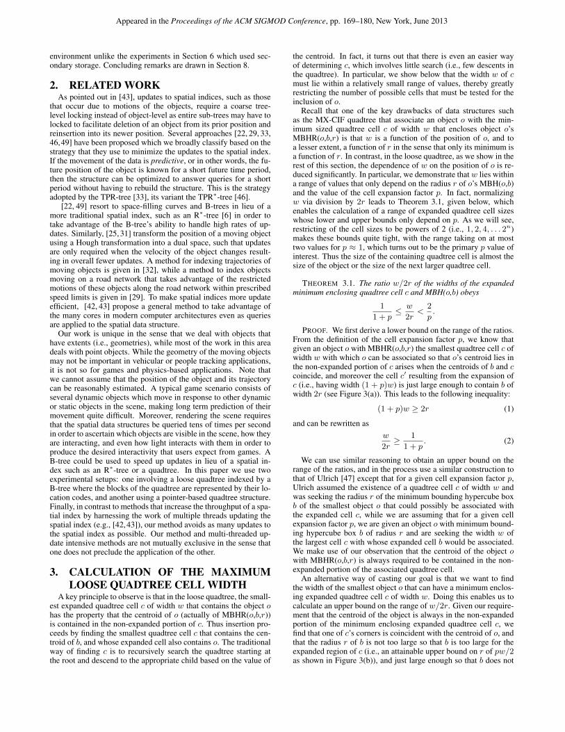
The cover fieldtree [12,13] and the more commonly known loosequadtree (octree) [47] are designed to overcome this independenceof the size of the minimum enclosing quadtree cell and the size ofthe object (see also the expanded MX-CIF quadtree [2], multipleshifted quadtree methods [7, 26, 27], and the partition fieldtree [12,13]). This is done by expanding the size of the space that is spannedby each quadtree cell c of widthw by a cell expansion factor p (p >0) so that the expanded cell is of width (1 + p) ·w and an object isassociated with its minimum enclosing expanded quadtree (octree)cell. The notion of an expanded quadtree cell can also be seen in thequadtree medial axis transform [34, 35]. For example, letting p =1, Figure 2 is the loose quadtree corresponding to the collection ofobjects in Figure 1(a) and its MX-CIF quadtree in Figure 1(b). Inthis example, there are only two differences between the loose andMX-CIF quadtrees:

1. Rectangle object E is associated with the SW child of theroot of the loose quadtree instead of with the root of the MX-CIF quadtree.

2. Rectangle object B is associated with the NW child of theNE child of the root of the loose quadtree instead of with theNE child of the root of the MX-CIF quadtree.

To further understand the loose quadtree and its behavior, seethe publicly available web site at http://www.cs.umd.edu/~hjs/loosequad/. The web site also contains a video titled“Crates and Barrels” that shows an N-body simulation containing14,000 objects. The video illustrates the improvement in in perfor-mance when using a loose quadtree over an MX-CIF quadtree.

(a) (b)

A

E

GF

D

CB

{G}

{A}

{B}

{E}{C,D}

{F}

Figure 2: (a) Cell decomposition induced by the loosequadtree for a collection of rectangle objects identicalto those in Figure 1, and (b) its tree representation(from [37]).

Ulrich [47] has shown that given a loose quadtree cell c of widthw and cell expansion factor p, the radius r of the minimum bound-ing hypercube box b of the smallest object o that could possibly beassociated with c must be greater than pw/4.

Our contribution is the realization that the real utility of the loosequadtree is best evaluated in terms of the inverse of the above re-lation as we are interested in minimizing the maximum possiblewidth w of c given an object o with minimum bounding hypercubebox b of radius r (i.e., half the length of a side of the hypercube)denoted by MBHR(o,b,r). This is because reducing w is the realmotivation and goal for the development of the loose quadtree asan alternative to the MX-CIF quadtree for which w can be as largeas the width of the underlying space. We achieve our goal in Sec-tion 3 by examining the range of the relative widths of c and b asthis provides a way of taking into account the constraints imposedby the fact that the range of values of w is limited to powers of 2.In particular, the novelty of our work lies in our showing this rangeto be just a function of p, and hence independent of the position ofo. Moreover, we prove that for p ≥ 0.5, the relative widths of c andb take on at most two values, and usually just one value for p ≥ 1.This makes updating the index very simple when objects are mov-ing as there are at most two possible new cells associated with amoved object, instead of log2 of the width of the space in whichthe objects are embedded (which can be as large as 16 assuming a216×216 embedding space as used by us). In other words, we haveshown how to update in O(1) time for p ≥ 0.5 which is of greatimportance as there is no longer a need to perform a search for theappropriate quadtree cell.

The rest of this paper is organized as follows. Section 2 discussesrelated work in the context of the moving object databases litera-ture. Section 3 shows how to achieve position independence for thewidth of the minimum enclosing quadtree cell c by examining therange of the relative widths of c and the minimum bounding hy-percube box b of object o, denoted by MBH(o,b), and also how totake into account the constraints imposed by the fact that the rangeof values of the width of c is limited to powers of 2. Section 4presents a cell insertion algorithm for the loose quadtree. Section 5discusses the ramifications of the results of Section 3. Section 6contains an experimental evaluation of the loose quadtree with re-spect to the extent that it needs to be updated on account of objectmotion for different values of p and object size distribution, Sec-tion 7 shows the results of using the Loose Quadtree in an N-bodysimulation which is typical of the type of functionality needed inmodern video games and hence is conducted in a main memory




environment unlike the experiments in Section 6 which used sec-ondary storage. Concluding remarks are drawn in Section 8.

2. RELATED WORKAs pointed out in [43], updates to spatial indices, such as those

that occur due to motions of the objects, require a coarse tree-level locking instead of object-level as entire sub-trees may have tolocked to facilitate deletion of an object from its prior position andreinsertion into its newer position. Several approaches [22, 29, 33,46,49] have been proposed which we broadly classify based on thestrategy that they use to minimize the updates to the spatial index.If the movement of the data is predictive, or in other words, the fu-ture position of the object is known for a short future time period,then the structure can be optimized to answer queries for a shortperiod without having to rebuild the structure. This is the strategyadopted by the TPR-tree [33], its variant the TPR∗-tree [46].

[22, 49] resort to space-filling curves and B-trees in lieu of amore traditional spatial index, such as an R∗-tree [6] in order totake advantage of the B-tree’s ability to handle high rates of up-dates. Similarly, [25, 31] transform the position of a moving objectusing a Hough transformation into a dual space, such that updatesare only required when the velocity of the object changes result-ing in overall fewer updates. A method for indexing trajectories ofmoving objects is given in [32], while a method to index objectsmoving on a road network that takes advantage of the restrictedmotions of these objects along the road network within prescribedspeed limits is given in [29]. To make spatial indices more updateefficient, [42, 43] propose a general method to take advantage ofthe many cores in modern computer architectures even as queriesare applied to the spatial data structure.

Our work is unique in the sense that we deal with objects thathave extents (i.e., geometries), while most of the work in this areadeals with point objects. While the geometry of the moving objectsmay not be important in vehicular or people tracking applications,it is not so for games and physics-based applications. Note thatwe cannot assume that the position of the object and its trajectorycan be reasonably estimated. A typical game scenario consists ofseveral dynamic objects which move in response to other dynamicor static objects in the scene, making long term prediction of theirmovement quite difficult. Moreover, rendering the scene requiresthat the spatial data structures be queried tens of times per secondin order to ascertain which objects are visible in the scene, how theyare interacting, and even how light interacts with them in order toproduce the desired interactivity that users expect from games. AB-tree could be used to speed up updates in lieu of a spatial in-dex such as an R∗-tree or a quadtree. In this paper we use twoexperimental setups: one involving a loose quadtree indexed by aB-tree where the blocks of the quadtree are represented by their lo-cation codes, and another using a pointer-based quadtree structure.Finally, in contrast to methods that increase the throughput of a spa-tial index by harnessing the work of multiple threads updating thespatial index (e.g., [42,43]), our method avoids as many updates tothe spatial index as possible. Our method and multi-threaded up-date intensive methods are not mutually exclusive in the sense thatone does not preclude the application of the other.

3. CALCULATION OF THE MAXIMUMLOOSE QUADTREE CELL WIDTH

A key principle to observe is that in the loose quadtree, the small-est expanded quadtree cell c of width w that contains the object ohas the property that the centroid of o (actually of MBHR(o,b,r))is contained in the non-expanded portion of c. Thus insertion pro-ceeds by finding the smallest quadtree cell c that contains the cen-troid of b, and whose expanded cell also contains o. The traditionalway of finding c is to recursively search the quadtree starting atthe root and descend to the appropriate child based on the value of

the centroid. In fact, it turns out that there is even an easier wayof determining c, which involves little search (i.e., few descents inthe quadtree). In particular, we show below that the width w of cmust lie within a relatively small range of values, thereby greatlyrestricting the number of possible cells that must be tested for theinclusion of o.

Recall that one of the key drawbacks of data structures suchas the MX-CIF quadtree that associate an object o with the min-imum sized quadtree cell c of width w that encloses object o’sMBHR(o,b,r) is that w is a function of the position of o, and toa lesser extent, a function of r in the sense that only its minimum isa function of r. In contrast, in the loose quadtree, as we show in therest of this section, the dependence of w on the position of o is re-duced significantly. In particular, we demonstrate thatw lies withina range of values that only depend on the radius r of o’s MBH(o,b)and the value of the cell expansion factor p. In fact, normalizingw via division by 2r leads to Theorem 3.1, given below, whichenables the calculation of a range of expanded quadtree cell sizeswhose lower and upper bounds only depend on p. As we will see,restricting of the cell sizes to be powers of 2 (i.e., 1, 2, 4, . . . 2n)makes these bounds quite tight, with the range taking on at mosttwo values for p ≈ 1, which turns out to be the primary p value ofinterest. Thus the size of the containing quadtree cell is almost thesize of the object or the size of the next larger quadtree cell.

THEOREM 3.1. The ratio w/2r of the widths of the expandedminimum enclosing quadtree cell c and MBH(o,b) obeys

1

1 + p≤ w

2r<

2

p.

PROOF. We first derive a lower bound on the range of the ratios.From the definition of the cell expansion factor p, we know thatgiven an object o with MBHR(o,b,r) the smallest quadtree cell c ofwidth w with which o can be associated so that o’s centroid lies inthe non-expanded portion of c arises when the centroids of b and ccoincide, and moreover the cell c′ resulting from the expansion ofc (i.e., having width (1 + p)w) is just large enough to contain b ofwidth 2r (see Figure 3(a)). This leads to the following inequality:

(1 + p)w ≥ 2r (1)

and can be rewritten asw

2r≥ 1

1 + p. (2)

We can use similar reasoning to obtain an upper bound on therange of the ratios, and in the process use a similar construction tothat of Ulrich [47] except that for a given cell expansion factor p,Ulrich assumed the existence of a quadtree cell c of width w andwas seeking the radius r of the minimum bounding hypercube boxb of the smallest object o that could possibly be associated withthe expanded cell c, while we are assuming that for a given cellexpansion factor p, we are given an object o with minimum bound-ing hypercube box b of radius r and are seeking the width w ofthe largest cell c with whose expanded cell b would be associated.We make use of our observation that the centroid of the object owith MBHR(o,b,r) is always required to be contained in the non-expanded portion of the associated quadtree cell.

An alternative way of casting our goal is that we want to findthe width of the smallest object o that can have a minimum enclos-ing expanded quadtree cell c of width w. Doing this enables us tocalculate an upper bound on the range of w/2r. Given our require-ment that the centroid of the object is always in the non-expandedportion of the minimum enclosing expanded quadtree cell c, wefind that one of c’s corners is coincident with the centroid of o, andthat the radius r of b is not too large so that b is too large for theexpanded region of c (i.e., an attainable upper bound on r of pw/2as shown in Figure 3(b)), and just large enough so that b does not


w w w

w

w

w

ww

w

w w w

w

w

w

w w w

(b)(a)

w(1+p)

pw/2w(1+p)

(c)

w(1+p)

pw/4

2r2r

2r

Figure 3: Assuming cell expansion factor p and an examples showing the (a) smallest ratio of the width w of thequadtree cell c associated with b and the width of b which is attained when the centroids of o and c coincide, andthe (b) lower and (c) upper bounds on the largest ratio attained when the centroid of o coincides with one of thecorners of c. Note that (c) is drawn at a different scale than (b).

fit in the expanded region of one of the subcells of c of width w/2(i.e., an unattainable lower lower bound on r of pw/4 as shown inFigure 3(c)). Equivalently, for this particular configuration, we saythat pw/4 = 2k−1 = r − δ′ < r ≤ 2k = pw/2 for some valueof k and δ′ > 0. Simplifying the notation by letting δ′ = δw/4,we have pw/4 = 2k−1 = r − δw/4 < r ≤ 2k = pw/2 for someδ > 0. Since the width w of c is the same for all values of r in thisrange, we point out that c’s width relative to that of b is maximizedwhen r takes on the value:

r = pw/4 + δw/4, δ > 0. (3)

which can be rewritten as:

w/2r =w

pw2

+ δw2

, δ > 0, (4)

w/2r =2

p+ δ<

2

p, (5)

w/2r <2

p. (6)

Combining relations 2 and 6 yields the range:

1

1 + p≤ w

2r<

2

p. (7)

We interpret Theorem 3.1 as follows. Without loss of generality,we assume that the quadtree cell corresponding to the root of theloose quadtree has length 2g , where g is an integer. This enablesus to avoid dealing with negative values of k, which is somewhatcounter intuitive, as would be the case were we to continue withthe unit hypercube assumption. In this case, all cells c in the loosequadtree have width w = 2k, such that k ≤ g is an integer. Now,for any given value x, let us define a function M(x) which deter-mines a k such that 2k−1 < x ≤ 2k, and returns the value 2k. Inother words,

M(x) = 2k, s.t. 2k−1 < x ≤ 2k. (8)

Moreover, we also have that

1 ≤ M(x)

x< 2. (9)

The rationale behind the function M(x) is that it quantizes x to thenext higher power of 2 unless it is already a power of 2. To explainthe utility of M(x) from a geometric point of view, consider aninput object R with a minimum bounding hypercube box of radiusr. We have that M(r) is the radius of the smallest quadtree cell(i.e., half the width) that can potentially contain R. We now derivethe minimum and maximum possible ratios of w/2r in terms ofM(.). Let us assume that 2r is a power of 2 which means thatthe minimum bounding box is a quadtree cell (i.e., M(r) = r).The number of levels of the loose quadtree spanned by the range[1/(p+1), 2/p) is upper-bounded by the number of integers of theform 2k, where k is an integer, and 2k/2r is contained in the range[1/(p + 1), 2/p). That is, we have just shown that the number oflevels spanned by the range in relation 7 cannot exceed V , whichis given by Lemma 3.1 below.

LEMMA 3.1. The number of levels in the loose quadtree atwhich the expanded minimum quadtree cell of the object could pos-sibly lie is upper bounded by V , where

V = log2(M(2/p))− log2(M(1/(p+ 1))). (10)

Now, let us make some observations on the possible ranges ofrelative cell widths on the basis of relations 7 and 10. First, for thedegenerate case of the MX-CIF quadtree, in which case no expan-sion takes place (i.e., p = 0), we have an unbounded upper boundon the range of values and a lower bound of 1. As p increases to-wards 1, the range of values decreases. For example, for p = 1/4,we have a range of relative cell widths [4/5, 8). This means that therelative cell widths of the set of possible quadtree cells containing agiven input rectangle R with a minimum bounding hypercube boxof radius r lie between [M(4/5) = 1,M(8) = 8) = {1, 2, 4}. Inother words, the quadtree cells containing R in the loose quadtreecan be of radiusM(r), 2M(r), and 4M(r) (i.e., half the width). Infact, these radii hold for all values of p such that 1/4 ≤ p < 1/2.

For p = 1/2, there are just two possible relative cell widthscorresponding to [M(2/3) = 1,M(4) = 4) = {1, 2}. Inother words, the associated quadtree cells of R can be either thequadtree cell of radius M(r) or of radius 2M(r). These radiihold for all values of p such that 1/2 ≤ p < 1. For p = 1,there are also just two possible relative cell widths correspondingto [M(1/2) = 1/2,M(2) = 2) = {1/2, 1}. In other words,the associated quadtree cells of R can be either the quadtree cell


of radius M(r), or can be of radius half of M(r). These radiihold for all values of p such that 1 ≤ p < 2. As p increasesbeyond 1, the number of possible ratios of relative cell widths os-cillates between one and two. In particular, for bpc = 2k − 1,where k ≥ 1 is an integer, the ratio w/2r takes on two values[M(1/2k) = 2−k,M(2/(2k − 1)) = 22−k), while for all othervalues of p (i.e., 2k ≤ p < 2k+1 − 1, where k ≥ 1 is an integer),w/2r takes on just one value M(1/2k) = 2−k.

4. INSERTION IN A LOOSE QUADTREEIn this section we show how Theorem 3.1 and Lemma 3.1 can

be used to derive a simple O(1) time object insertion algorithmfor the loose quadtree. We first give an example of the algorithmusing p = 1/4. From Theorem 3.1, we have that the quadtreecells containing a given input rectangle object o with a minimumbounding hypercube box of radius r can be associated with oneof three possible cells of radius M(r), 2M(r), and 4M(r). Theinsertion algorithm proceeds as follows. We first find a cell b ofradius M(r), such that it contains the centroid of o. This can bedone in O(1) time by noting that M(r) = 2dlog2 re. At this point,we have that either b, the parent of b (say b′) of radius 2M(r), orthe parent of b′ (say b”) of radius 4M(r) contains o and we inserto in the smallest one whose expanded region contains o.

The actual insertion algorithm is given by procedure Loose-QuadtreeInsert below. It uses Lemma 3.1 to determine thenumber of quadtree cells and their corresponding sizes that are tobe checked in the loop in lines 8–22 to determine the minimum-sized quadtree cell that is to contain the object to be inserted. Thealgorithm does not assume that the loose quadtree is representedas a tree structure with out degree 4 (8 for a loose octree in threedimensions). Instead, it assumes the use of a pointerless quadtreerepresentation (e.g., [14, 37]) that just keeps track of the leaf nodes(i.e., cells) of the loose quadtree which are represented using, forexample, a number, termed a locational code (referred to as theMorton Representation [28] in Section 6), that uniquely identifieseach leaf node. This number can be formed by concatenating thesize of the cell, say i for a cell of width 2i, with a number j result-ing from interleaving the binary representations of the coordinatevalues of a predefined corner such as the lower-left corner assum-ing that the origin of the underlying space is at the lower-left corner(e.g., (a, b) in two dimensions) so that i is at the right of j. The col-lection of these numbers can be represented using any access struc-ture including binary search trees, balanced binary search trees, B-trees, etc. although our implementation in the experimental setupin Section 6 uses a B-tree. Thus the role of LooseQuadtree-Insert is simply to create records for the loose quadtree whichconsist of the locational code and a reference to the object so thatwe can differentiate between objects that are associated with thesame leaf node (i.e., cell) of the loose quadtree. In this case, thecell is replicated in the access structure.

1 pointer loose_quadtree_block procedure Loose-QuadtreeInsert(p,o)

2 /* Given a loose quadtree with expansion factor p, create andreturn a loose quadtree record for object o which containsthe object and its locational code. Object o is represented bya record of type object having the fields XCent, YCent,and MbbRadius corresponding to the x and y coordi-nate values of o’s centroid, and the radius of o’s minimumbounding hypercube box. The function M(r) returns theinteger 2k such that 2k−1 < r ≤ 2k. The locational codeis obtained by applying bit interleaving to the binary repre-sentations of x low and ylow , the x and y coordinate valuesof the lower-left corner of the loose quadtree cell b of widthw which contains o and concatenating it to the depth of b

(i.e., log2(w)) and its value is a pointer to object o. If sev-eral objects are associated with the same cell of the loosequadtree, then the cell is replicated. These replicated loosequadtree cells are differentiated by virtue of the objects thatare associated with them. The actual loose quadtree recordfor the cell including its locational code is constructed byprocedure FormBlock (not given here). Note the use of“÷” to denote integer division, “/” to denote real division,and ↑ to denote exponentiation. */

3 value real p4 value object o5 real r6 integer i, w, xlow , ylow

7 r ←MbbRadius(o)8 for i← log2(M(1/(p+ 1))) step 19 until log2(M(2/p))− 1 do

10 /* Calculate width of smallest possible cell b containing o*/

11 w ← (2 ↑ (i+ 1)) ∗M(r)12 /* Determine b’s lower-left corner (xlow , ylow ) */13 xlow ← (XCent(o)÷ w) ∗ w14 ylow ← (YCent(o)÷ w) ∗ w15 /* Determine if b’s expanded region contains o */16 if xlow − p ∗ w/2 ≤ XCent(o)− r and17 XCent(o) + r ≤ xlow + (1 + p/2) ∗ w and18 ylow − p ∗ w/2 ≤ YCent(o)− r and19 YCent(o) + r ≤ ylow + (1 + p/2) ∗ w20 then exit_for_loop21 endif22 enddo23 return(FormBlock(xlow , ylow , w, o))

5. DISCUSSIONThe calculations of the possible containing quadtree cell widths

for p = 1/4, p = 1/2, and p = 1 lead to the observation that as ptakes larger values (even for p as small as 1/4), the loose quadtreetreats the input objects as if they are points and it is their centroidthat determines their associated quadtree cell, while their size andthe value of the cell expansion factor determine the size of theirassociated quadtree cell. Actually, the above statement must betempered a bit. In particular, although it implies that the positionof object o is not a factor in the determination of the width w of theexpanded quadtree cell c with which o’s MBH(o,b) is associated,this is not quite true as the existence of a range of values for theratio w/2r of the widths of c and b is a direct result of the variationin the position of o along with that of the value of p. However, aswe showed above, for values of p ≥ 1/2, the values of the ratio ofthe widths of c and b take on at most two values which differ by onewhere, in the case of p ≥ 1, the only reason for the two possibleratio values is the fact that at times p takes on a value which is oneless than a power of 2.

At this point, it is appropriate to ask what value p should oneuse. The answer must bear in mind that as p gets large, the radii(i.e., half the width) of the associated expanded quadtree cells getlarger and thus they overlap adjacent quadtree cells of half the ra-dius for p = 1 and of equal radius for p = 2, and even greater radiias p increases further. On the other hand, as p approaches 0, theradii of the quadtree cells associated with object o are increasinglydependent on the position of the centroid of object o and can getdisproportionately large independent of the radius of o’s minimumbounding hypercube box. The cardinality of the set of possible val-ues of these radii is minimized at 1 when p ≥ 2 with the exceptionof p = 2k − 1 for integer values of k in which case the cardinal-ity of the set is 2 corresponding to radius values 2i and 2i+1 for


some integer i. Clearly, there is no point in letting p get largerthan 2 in which case the radius of the associated quadtree cell ispre-determined and depends solely on the value of the radius of o’sminimum bounding hypercube box.

Thus we remain with the range 1/2 ≤ p < 2 for which the cardi-nality of the set of possible values of the radii of the quadtree cellsis 2 corresponding to radius values 2i and 2i+1 for some integeri. Our rationale for choosing p in this range is that the expandedquadtree cells are not so large as is the case for p = 2 and hencethe extent of the overlap with adjacent quadtree cells is reduced,while the burden of having two possible radii for the quadtree cellsis not great. Of course, procedure LooseQuadtreeInsert inSection 4 is not as simple for p = 1 as it is for p = 2, in whichcase there is no need for the loop in lines 8–22. Nevertheless, forp = 1, the loop in lines 8–22 need only be executed twice, whichis still quite simple. Ulrich [47] lets p = 1, while results of ourexperiments described in Section 6 make a case for choosing p tobe infinitesimally smaller than 1. It is important to observe that allof the results that we have described hold for loose quadtrees of ar-bitrary dimension (e.g., three dimensions such as the loose octree)as they are all formulated in terms of the radii of the quadtree cells.

Algorithms that make use of the loose quadtree are simplifiedby our observation that the centroid of object o (actually of o’sMBHR(o,b,r) is always contained in the non-expanded portion ofthe quadtree cell c with which o is associated. However, there arescenarios where users may wish to violate this property. For ex-ample, for certain values of r and p, r may be sufficiently smallso that both the centroid of o lies in the expanded portion of c ando still fits in the expanded cell c. This situation is desirable whenusers want to move o as much as possible without having to asso-ciate it with another quadtree cell just because o’s centroid is nolonger in the non-expanded region of c. Interestingly, this modi-fication does not change the ranges of relative cell widths as theexample in Figure 3(c) still corresponds to the largest value of theratio. The difference is that now the motion of the object so thatthe centroid of o is also in the expanded portion of c does not resultin the association of o with another cell as long as o lies entirely inthe expanded portion of c. Of course, this complicates subsequentsearches (as well as delete operations), as now instead of just look-ing for a cell whose non-expanded portion contains the centroid ofo, we must examine all possible cells whose expanded cells cancontain o. Notice that in essence, we have transformed the searchproblem from one involving points (i.e., centroids of the objects)to one involving regions (i.e., the minimum bounding hypercubeboxes of the objects).

6. EXPERIMENTAL EVALUATIONExperiments were run on a Linux (2.6.18) quad 1.86 GHz Xeon

server with four gigabyte of RAM. The algorithms were imple-mented using GNU C++. The experiments studied the behaviorof loose quadtrees in an environment where the objects are in mo-tion. Our experimental setup consisted of a large collection of rect-angle objects. For most, but not all, of our experiments, we usedrandom rectangle data obtained by generating their centroid andextents at random, which is equivalent to the method used by Ul-rich [47]. Each object (i.e, rectangle) in the collection is associ-ated with its minimum enclosing quadtree cell (actually minimumenclosing expanded quadtree cell), which is represented by its bit-interleaved Morton representation [28]. The Morton representationis indexed using a B-tree index, which is referred to as a linearquadtree [14, 37].

In our setup, we use a non-spatial index (e.g., array, B-tree, Hash)to index the input objects by their identifier and a spatial index (i.e.,loose quadtree in our case represented as a linear quadtree) to in-dex the current positions of the objects. As an object’s positionchanges, we first update its current position using the non-spatial

index. This operation is fairly quick as updating the position ofthe object requires no modification to the non-spatial index itself.Next, we must update the spatial index which poses a real com-putational bottleneck as even small changes in the position of theobject result in an update to the index. We remedy this problem toa limited extent by representing an object by the quadtree cell withwhich it is associated (not necessarily containing it as the loosequadtree permits objects to be associated with smaller cells). Thismeans that the index does not store the exact geometry of the ob-ject. However, given that we know that the ratio of the sizes of theobject’s minimum enclosing expanded quadtree cell and of the ob-ject is bounded by a small value which is a function of p, we are insome sense implicitly recording the geometry of the object in theindex. Moreover, the Morton representation that is stored in the B-tree contains a reference to the actual object, which is stored in anarray and also indexed by the non-spatial index in order to facilitatequick updates, when necessary.

In this respect, the loose quadtree is distinguished from all otherspatial indices, such as an R-tree, that explicitly store the positionsof objects (i.e., rectangles). This means that when the position ofan object changes, in the case of an R-tree and related spatial in-dices, we would have to always update the indices as they dependon the minimum bounding hypercube boxes of the objects whichhave changed, while in the case of the loose quadtrees, we onlyneed to update the index if if the object is associated with a dif-ferent quadtree cell. This property of the loose quadtree makes itattractive for serving as a spatial index for moving object applica-tions. In contrast, as we pointed out, updates in spatial indices suchas the R-tree, as well as other related spatiotemporal indices, willoften require a complete rebuild step when the position of the ob-ject changes, which is quite complicated. Nevertheless, for the sakeof completeness, we provide a comparison of comparison of loosequadtree with a suitable implementation of a R-tree in Section 7.

We ran a number of experiments to test the sensitivity of theloose quadtree to the motion of the objects that it stores. Weused a collection of one million randomly generated rectangles in atwo-dimensional space, which were stored in a B-tree based loosequadtree index. Our implementation of the B-tree is single threadedwith a node size of 8 kb that can store up to 64 objects per node.Furthermore, we cache 10% of the nodes in an in-memory cache.The non-spatial index is an in-memory array indexed by the ob-ject identifier. For this set of experiments we chose a disk-baseddata structure such as a B-tree to index the objects instead of an in-memory spatial data structure. The B-tree is better than the pointer-based quadtree in the sense that it provides access to each quadtreecell (node) in the tree using its locational code in constant time (i.e.,time proportional to the height of the B-tree, which we view as aconstant) whereas in the pointer-based quadtree our access time isproportional to the base 2 logarithm of the width (i.e., maximumdepth) of the underlying embedding space.

We let the expansion factor p vary between 0 and 5. Recall thatfor the case p = 0, the loose quadtree corresponds to an MX-CIF quadtree. We first built an index for all the objects in a loosequadtree for a given p. Next, we translated the objects in order tomimic a moving object application. If the translations resulted inan object being associated with a different quadtree cell, then weupdated the index, which involves deleting an entry from the B-tree index and adding a new entry corresponding to the minimumexpanded quadtree cell containing the object after the translation.We tabulated the number of objects for which the index needed tobe updated. We controlled the motion of the objects using a values, denoting the maximum translation of the object across a singledimension. For example, suppose that s is 5%, then all of the rect-angles are translated across each of the dimensions by a value thatis at most 5% of its side length across each of the dimensions.

In order to provide a better understanding of the effect of motionon the loose quadtree index, we distinguish between two types of


motion, namely uniform and fixed translations. In the case of auniform translation, the motion is controlled by a random variable,which is bounded by s. In other words, all the objects are subjectedto different translations, where the translation across any dimensionis less than s. In the case of a fixed translation, all of the objects aretranslated by a fixed value (i.e., s) across each of the dimensions,which basically represents the worst case scenario (in terms of themaximum amount of motion) of any moving object application.

75 50

25

10

5

1

0.5

5 2 1 0.5 0.2 0.1

% R

eins

ertio

ns (

log

scal

e)

Looseness Factor p (log scale)

s=0.40%s=1.00%s=2.00%s=4.00%s=10.0%s=50.0%s=100.%

(a)

100 75 50

25

10

5

1

0.5 5 2 1 0.5 0.2 0.1

% R

eins

ertio

ns (

log

scal

e)


s=0.40%s=1.00%s=2.00%s=4.00%s=10.0%s=50.0%s=100.%

(b)

Figure 4: Reinsertion rates for two-dimensional rectan-gle input for varying values of p and s with δ = 10, fora) uniform and b) fixed translations.

Finally, we also varied the sizes of the input rectangle objects byusing the value δ, which denotes the ratio of the largest side lengthof a rectangle object in the data set to the smallest side length ofa rectangle object in the data set. It should be clear that a largevalue of δ means a large range of rectangle object sizes, while asmall value of δ means that the rectangle objects are more or lessof the same size. All of the experiments whose results we presentvaried one or more of these variables to showcase the utility ofloose quadtrees for moving object applications. Note that this is afar more extensive experimental evaluation than the one conductedby Ulrich [47] who only studied the loose quadtree’s behavior forculling operations and only compared the p = 0 and p = 1 cases.

Our first experiment considered the case of one million two-dimensional rectangle objects for values of p ranging between 0and 5, and values of s ranging between 0.40% and 100%. The valueof δ was kept constant at 10. Figure 4 shows the percentage of ob-jects that required reinsertion as a function of p, while the differentcurves in the plot show the behavior of the loose quadtree indexfor different values of s. As expected, the percentage of objectsthat require reinsertion increases as s increases. From the figure,we observe that this percentage increases with p with a precipitousdrop at p = 0.999 where the results are comparable to p = 0. Fig-ure 5 provides a more vivid illustration of the comparability of theresults for p = 0.999 with those for p = 0 by showing the result ofnormalizing the reinsertion rates for the different values of p and svis-a-vis those for p = 0.999. Here we see that the reinsertion ratefor p = 0.999 is superior to the other values of p for all reasonablevalues of s (i.e., less than s <50%). It is interesting to note that forall values of s, for small values of p, this percentage increases withp with a local maximum at around p = 0.5, at which time it hasa precipitous drop at p = 0.999 where the results are comparableto p = 0, and then increases sharply for p = 1, and continues toincrease, but at a lesser rate, as p continues to increase (i.e., p >1).This phenomenon is explained in greater detail below.

The percentage of objects requiring reinsertion is relatively lowat p = 0 since the range of the values of the side lengths of theminimum enclosing quadtree cells is large as is also the value ofthe maximum side length. This means that objects often have alarge area in which to move without requiring reinsertion. As p in-creases, we observe that the range of values of the side lengths ofthe minimum enclosing expanded quadtree cells become increas-

5

4

3

2

1.5 1.3

1 0.9 0.8

5 2 1 0.5 0.2 0.1

Nor

mal

ized

Rei

nser

tions

(lo

g sc

ale)


s=0.40%s=1.00%s=2.00%s=4.00%s=10.0%s=50.0%s=100.%

(a)

5

4

3

2

1.2 1

5 2 1 0.5 0.2 0.1

Nor

mal

ized

Rei

nser

tions

(lo

g sc

ale)


s=0.40%s=1.00%s=2.00%s=4.00%s=10.0%s=50.0%s=100.%

(b)

Figure 5: Reinsertions for two-dimensional rectangleinput for varying values of p and s with δ = 10, normal-ized with the reinsertion rate for p = 0.999 for a) uniformand b) fixed translations.

0.5 <= p < 1

0.25 <= p < 0.5

1 <= p < 2

2w 2w

2w

2w

2w

2w

2w 2w

2w

2w

2w

2w

4w

4ww w w

w

w

w

w w w

w

w

w

w w w

w

w

ww

Object

wQuadtree block

QuadtreeLoose

block

Legend:

0.5w

0.5w

(a)(b)

(b)

(b)

(c)

(c)(d)

w(1+p)

2r

Figure 6: Illustration of the variation of the relative sizesof the minimum enclosing expanded quadtree cells andof the minimum bounding hypercube boxes of the ob-jects with respect to different ranges of values of p:(first row) 0.25≤p<0.5, (second row) 0.5≤p<1, and(third row) 1≤p<2.

ingly smaller, which means that the area in which the objects canmove without requiring reinsertion gets smaller. Figure 6 illustratesthis observation using an example object with minimum boundinghypercube box of radius r. In particular, we can see that for valuesof p in the range [0.25, 0.5), the side length of the minimum enclos-ing expanded quadtree cell is either 2, 4, or 8 times the radius of theminimum bounding hypercube box of the object (first row of Fig-ure 6) ; while for values of p in the ranges [0.5, 1), the side lengthof the minimum enclosing expanded quadtree cell is either 2 or 4times the radius of the minimum bounding hypercube box of theobject (second row of Figure 6); and for values of p in the ranges[1, 2) the side length of the minimum enclosing expanded quadtreecell is either 1 or 2 times the radius of the minimum boundinghypercube box of the object (third row of Figure 6). Notice thatthe percentage of objects requiring reinsertion starts to decrease atp = 0.5 with a minimum at p = 0.999. This is because at p = 0.5there are only two choices for the size of the minimum enclosingexpanded quadtree cell, having eliminated the cell with side length8 times the radius of the minimum bounding hypercube box of theobject. Moreover, the number of objects associated with the elim-


inated cell are relatively small. On the other hand, at p = 1, thereare again only two choices for the minimum enclosing expandedquadtree cell, but now a large such cell is replaced by one with aquarter of its area thereby greatly limiting the ability of the objectsto move without requiring reinsertion. The pattern of increasingpercentages requiring reinsertion continues unabated for p > 1 aswe have increasingly smaller replacement cells with saw-tooth likebehavior in the neighborhood of p = 2k.

0

0.5

1

1.5

2

2.5

3

3.5

5 2 1 0.5 0.2 0.1

Upd

ates

(m

illio

ns/s

econ

d)


(a)

0.1

1

10

5 2 1 0.5 0.2 0.1

Upd

ates

(m

illio

ns/s

econ

d)


s=0.40%s=1.00%s=2.00%s=4.00%s=10.0%s=50.0%s=100.%

(b)

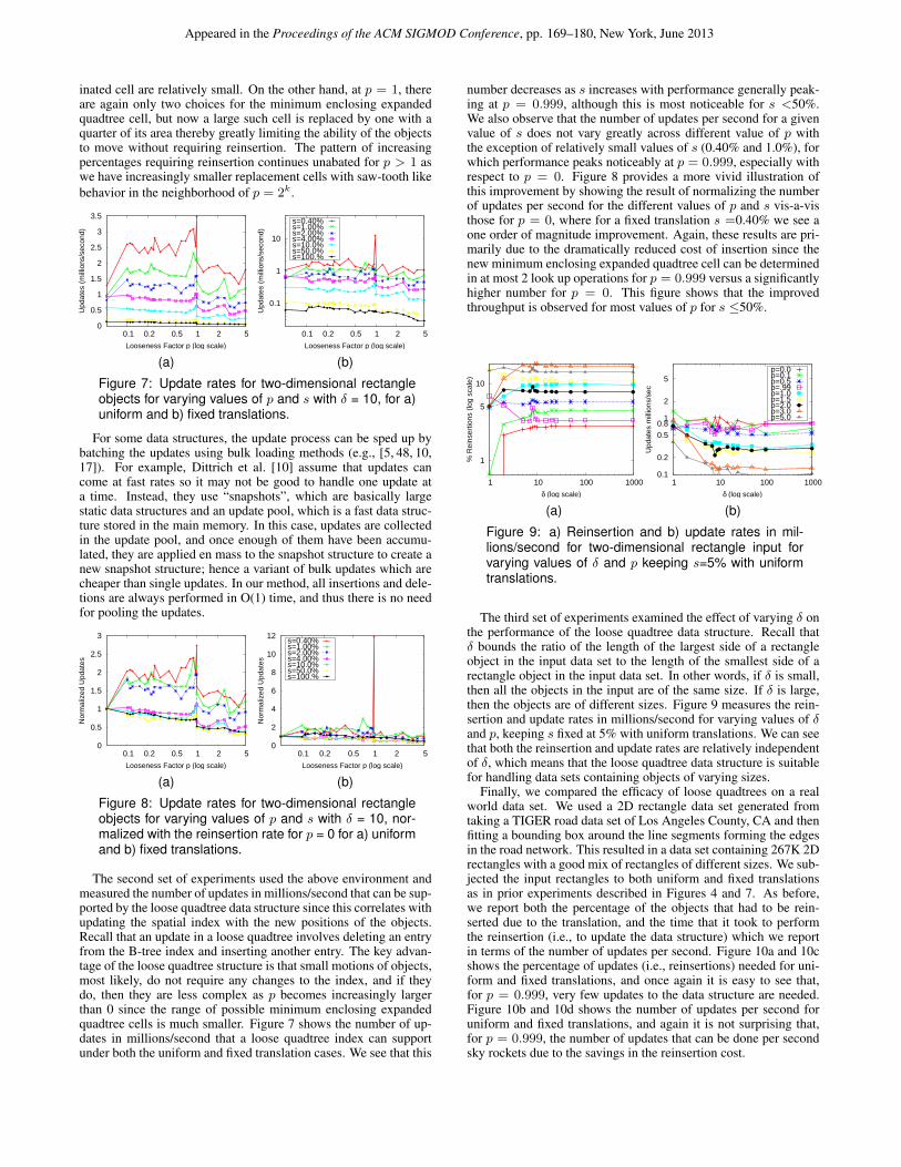
Figure 7: Update rates for two-dimensional rectangleobjects for varying values of p and s with δ = 10, for a)uniform and b) fixed translations.

For some data structures, the update process can be sped up bybatching the updates using bulk loading methods (e.g., [5, 48, 10,17]). For example, Dittrich et al. [10] assume that updates cancome at fast rates so it may not be good to handle one update ata time. Instead, they use “snapshots”, which are basically largestatic data structures and an update pool, which is a fast data struc-ture stored in the main memory. In this case, updates are collectedin the update pool, and once enough of them have been accumu-lated, they are applied en mass to the snapshot structure to create anew snapshot structure; hence a variant of bulk updates which arecheaper than single updates. In our method, all insertions and dele-tions are always performed in O(1) time, and thus there is no needfor pooling the updates.

0

0.5

1

1.5

2

2.5

3

5 2 1 0.5 0.2 0.1

Nor

mal

ized

Upd

ates


(a)

0

2

4

6

8

10

12

5 2 1 0.5 0.2 0.1

Nor

mal

ized

Upd

ates


s=0.40%s=1.00%s=2.00%s=4.00%s=10.0%s=50.0%s=100.%

(b)

Figure 8: Update rates for two-dimensional rectangleobjects for varying values of p and s with δ = 10, nor-malized with the reinsertion rate for p = 0 for a) uniformand b) fixed translations.

The second set of experiments used the above environment andmeasured the number of updates in millions/second that can be sup-ported by the loose quadtree data structure since this correlates withupdating the spatial index with the new positions of the objects.Recall that an update in a loose quadtree involves deleting an entryfrom the B-tree index and inserting another entry. The key advan-tage of the loose quadtree structure is that small motions of objects,most likely, do not require any changes to the index, and if theydo, then they are less complex as p becomes increasingly largerthan 0 since the range of possible minimum enclosing expandedquadtree cells is much smaller. Figure 7 shows the number of up-dates in millions/second that a loose quadtree index can supportunder both the uniform and fixed translation cases. We see that this

number decreases as s increases with performance generally peak-ing at p = 0.999, although this is most noticeable for s <50%.We also observe that the number of updates per second for a givenvalue of s does not vary greatly across different value of p withthe exception of relatively small values of s (0.40% and 1.0%), forwhich performance peaks noticeably at p = 0.999, especially withrespect to p = 0. Figure 8 provides a more vivid illustration ofthis improvement by showing the result of normalizing the numberof updates per second for the different values of p and s vis-a-visthose for p = 0, where for a fixed translation s =0.40% we see aone order of magnitude improvement. Again, these results are pri-marily due to the dramatically reduced cost of insertion since thenew minimum enclosing expanded quadtree cell can be determinedin at most 2 look up operations for p = 0.999 versus a significantlyhigher number for p = 0. This figure shows that the improvedthroughput is observed for most values of p for s ≤50%.

10

5

1

1 10 100 1000

% R

eins

ertio

ns (

log

scal

e)

δ (log scale)

(a)

5

2

1 0.8 0.5

0.2

0.1 1 10 100 1000

Upd

ates

mill

ions

/sec

δ (log scale)

p=0.0p=0.1p=0.5p=.99p=1.0p=1.5p=2.0p=3.0p=5.0

(b)

Figure 9: a) Reinsertion and b) update rates in mil-lions/second for two-dimensional rectangle input forvarying values of δ and p keeping s=5% with uniformtranslations.

The third set of experiments examined the effect of varying δ onthe performance of the loose quadtree data structure. Recall thatδ bounds the ratio of the length of the largest side of a rectangleobject in the input data set to the length of the smallest side of arectangle object in the input data set. In other words, if δ is small,then all the objects in the input are of the same size. If δ is large,then the objects are of different sizes. Figure 9 measures the rein-sertion and update rates in millions/second for varying values of δand p, keeping s fixed at 5% with uniform translations. We can seethat both the reinsertion and update rates are relatively independentof δ, which means that the loose quadtree data structure is suitablefor handling data sets containing objects of varying sizes.

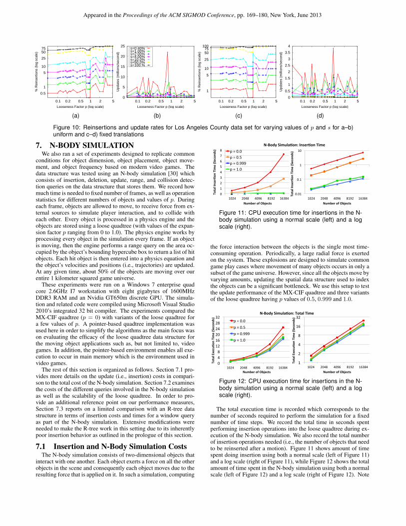
Finally, we compared the efficacy of loose quadtrees on a realworld data set. We used a 2D rectangle data set generated fromtaking a TIGER road data set of Los Angeles County, CA and thenfitting a bounding box around the line segments forming the edgesin the road network. This resulted in a data set containing 267K 2Drectangles with a good mix of rectangles of different sizes. We sub-jected the input rectangles to both uniform and fixed translationsas in prior experiments described in Figures 4 and 7. As before,we report both the percentage of the objects that had to be rein-serted due to the translation, and the time that it took to performthe reinsertion (i.e., to update the data structure) which we reportin terms of the number of updates per second. Figure 10a and 10cshows the percentage of updates (i.e., reinsertions) needed for uni-form and fixed translations, and once again it is easy to see that,for p = 0.999, very few updates to the data structure are needed.Figure 10b and 10d shows the number of updates per second foruniform and fixed translations, and again it is not surprising that,for p = 0.999, the number of updates that can be done per secondsky rockets due to the savings in the reinsertion cost.


75 50

25

10

5

1

0.5

5 2 1 0.5 0.2 0.1

% R

eins

ertio

ns (

log

scal

e)


(a)

0

5

10

15

20

25

5 2 1 0.5 0.2 0.1

Upd

ates

(m

illio

ns/s

econ

d)


s=0.40%s=1.00%s=2.00%s=4.00%s=10.0%s=50.0%s=100.%

(b)

100 75 50

25

10

5

1

5 2 1 0.5 0.2 0.1

% R

eins

ertio

ns (

log

scal

e)


(c)

0

0.5

1

1.5

2

2.5

3

3.5

4

5 2 1 0.5 0.2 0.1

Upd

ates

(m

illio

ns/s

econ

d)


(d)

Figure 10: Reinsertions and update rates for Los Angeles County data set for varying values of p and s for a–b)uniform and c–d) fixed translations

7. N-BODY SIMULATIONWe also ran a set of experiments designed to replicate common

conditions for object dimension, object placement, object move-ment, and object frequency based on modern video games. Thedata structure was tested using an N-body simulation [30] whichconsists of insertion, deletion, update, range, and collision detec-tion queries on the data structure that stores them. We record howmuch time is needed to fixed number of frames, as well as operationstatistics for different numbers of objects and values of p. Duringeach frame, objects are allowed to move, to receive force from ex-ternal sources to simulate player interaction, and to collide witheach other. Every object is processed in a physics engine and theobjects are stored using a loose quadtree (with values of the expan-sion factor p ranging from 0 to 1.0). The physics engine works byprocessing every object in the simulation every frame. If an objectis moving, then the engine performs a range query on the area oc-cupied by the object’s bounding hypercube box to return a list of hitobjects. Each hit object is then entered into a physics equation andthe object’s velocities and positions (i.e., trajectories) are updated.At any given time, about 50% of the objects are moving over ourentire 1 kilometer squared game universe.

These experiments were run on a Windows 7 enterprise quadcore 2.6GHz I7 workstation with eight gigabytes of 1600MHzDDR3 RAM and an Nvidia GT650m discrete GPU. The simula-tion and related code were compiled using Microsoft Visual Studio2010’s integrated 32 bit compiler. The experiments compared theMX-CIF quadtree (p = 0) with variants of the loose quadtree fora few values of p. A pointer-based quadtree implementation wasused here in order to simplify the algorithms as the main focus wason evaluating the efficacy of the loose quadtree data structure forthe moving object applications such as, but not limited to, videogames. In addition, the pointer-based environment enables all exe-cution to occur in main memory which is the environment used invideo games.

The rest of this section is organized as follows. Section 7.1 pro-vides more details on the update (i.e., insertion) costs in compari-son to the total cost of the N-body simulation. Section 7.2 examinesthe costs of the different queries involved in the N-body simulationas well as the scalability of the loose quadtree. In order to pro-vide an additional reference point on our performance measures,Section 7.3 reports on a limited comparison with an R-tree datastructure in terms of insertion costs and times for a window queryas part of the N-body simulation. Extensive modifications wereneeded to make the R-tree work in this setting due to its inherentlypoor insertion behavior as outlined in the prologue of this section.

7.1 Insertion and N-Body Simulation CostsThe N-body simulation consists of two-dimensional objects that

interact with one another. Each object exerts a force on all the otherobjects in the scene and consequently each object moves due to theresulting force that is applied on it. In such a simulation, computing

0 1 2 3 4 5 6 7 8

1024 2048 4096 8192 16384

Total Inser,o

n Time (Secon

ds)

Number of Objects

p = 0.0 p = 0.5 p = 0.999 p = 1.0

0.01

0.1

1

10

1024 2048 4096 8192 16384

Total Inser,o

n Time (Secon

ds)

Number of Objects

N-‐Body Simula,on: Inser,on Time

Figure 11: CPU execution time for insertions in the N-body simulation using a normal scale (left) and a logscale (right).

the force interaction between the objects is the single most time-consuming operation. Periodically, a large radial force is exertedon the system. These explosions are designed to simulate commongame play cases where movement of many objects occurs in only asubset of the game universe. However, since all the objects move byvarying amounts, updating the spatial data structure used to indexthe objects can be a significant bottleneck. We use this setup to testthe update performance of the MX-CIF quadtree and three variantsof the loose quadtree having p values of 0.5, 0.999 and 1.0.

0 4 8

12 16 20 24 28 32

1024 2048 4096 8192 16384

Total Execu,o

n Time (Secon

ds)

Number of Objects

p = 0.0 p = 0.5 p = 0.999 p = 1.0

1

2

4

8

16

32

1024 2048 4096 8192 16384

Total Execu,o

n Time (Secon

ds)

Number of Objects

N-‐Body Simula,on: Total Time

Figure 12: CPU execution time for insertions in the N-body simulation using a normal scale (left) and a logscale (right).

The total execution time is recorded which corresponds to thenumber of seconds required to perform the simulation for a fixednumber of time steps. We record the total time in seconds spentperforming insertion operations into the loose quadtree during ex-ecution of the N-body simulation. We also record the total numberof insertion operations needed (i.e., the number of objects that needto be reinserted after a motion). Figure 11 shows amount of timespent doing insertion using both a normal scale (left of Figure 11)and a log scale (right of Figure 11), while Figure 12 shows the totalamount of time spent in the N-body simulation using both a normalscale (left of Figure 12) and a log scale (right of Figure 12). Note


the similar behavior for the four variants with p = 0.999 perform-ing the best. In fact, there is a one half order of magnitude differ-ence in the insertion and total N-body simulation execution timesbetween p = 0 and p = 0.999. It is interesting to note that the dif-ference between the total execution times of the N-body simulationwith the use of p = 0.999 versus with the use of p = 0 is accountedfor by the savings in the insertion costs (approximately 7 seconds).Figure 13 shows the relatively large reduction in the number of ob-jects that need reinsertion when using p = 0.999 vis-a-vis p = 0.It is also interesting to note that all of the log plots show a linearrelationship which means that all of the statistics that we collectedobey a power law of y = axb where a and b are constants with bvarying between 1.60 and 1.75. It is clear from this data that theloose quadtree outperforms the MX-CIF quadtree (p = 0), and thatthe value of p = 0.999 leads to better performance than p = 1.In fact, we see almost two orders of magnitude less insertions forp = 0.999 vis-a-vis p = 0. In the case of p = 1.0 and p = 0.999we see reductions as high as 30% in both the total number of inser-tions (Figure 13) and time spent in insertions (Figure 11), and ashigh as 10% in the total execution time of the N-body simulation,which is less as expected since we are looking at the total execu-tion time which involves more operations than insertions, but is stillvery good.

1000

10000

100000

1000000

10000000

1024 2048 4096 8192 16384

Toptal Num

ber o

f Inser2o

ns

Number of Objects

p = 0.0 p = 0.5 p = 0.999 p = 1.0

Figure 13: Number of insertions in the N-body simula-tion using a log scale.

7.2 Query Performance and ScalabilityWe now examine the performance of the loose quadtree for the

queries that form the key geometric operations in an N-body simu-lation. Our motivation is to show that the good update performanceof the loose quadtree (i.e., minimization of reinsertions upon ob-ject motion) does not come at the expense of query performance,and that it scales. In order to do this, our first set of experimentsmeasured the time taken to perform a number of different queriesas well as recorded the number of blocks and objects in the loosequadtree that are visited by each query. Our second set of experi-ments examines the performance of the loose quadtree on simula-tions with varying sizes of objects. In particular, we show that theloose quadtrees can scale to handle really large simulations way be-yond the limitations of the MX-CIF quadtree (i.e., a loose quadtreewith p = 0).

In order to test the query performance of the data structures, weuse a different environment than the one in Section 7.1. In partic-ular, we recreate a game environment to simulate a complex 3Dscene. In this scenario, the objects do not exert force on one an-other but move due to gravity. Hence, the bottleneck in this en-vironment is not computing the inter-object forces but rather cap-turing the interactions between the objects as they collide with oneanother. Capturing these interactions between the objects requiresknowledge of which objects are in close proximity to which otherobjects in the scene. All objects in the environment are updateddynamically using a physics simulation solver. Furthermore, wealso render the scene which requires the application of geometrical

operations such as ray tracing, view frustum culling and windowqueries on the spatial data structures.

We note that the time taken to compute each time step in thesimulation is roughly broken down as follows: About 70% of thetime is spent on updating the data structure, 20% of the time is spenton performing geometric operations such as frustum culling, raytracing, window and nearest neighbor search, while the remaining10% of the time is spent on rendering the scene. Note that renderingis GPU assisted, so that the 10% time only corresponds to the timeneeded to transfer the objects to the GPU, which makes it relativelyindependent of the complexity of the scene. Moreover, the timetaken to render the scene is also common to all the data structuresthat we examine in this section.

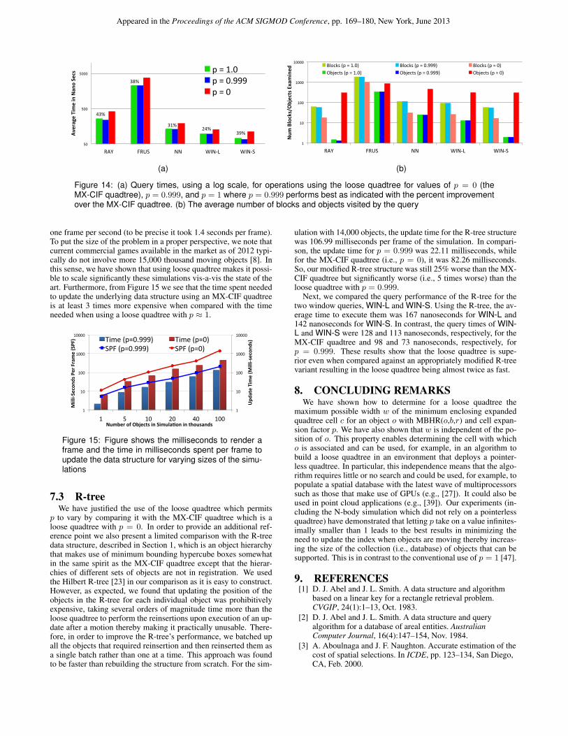
Below, we examine the time needed to execute a number ofqueries as part of an N-body simulation with 14,000 dynamic ob-jects. Figure 14a shows the average times in nanoseconds neededto perform each of the queries, while Figure 14b shows the averagenumber of blocks and objects visited while processing the queries.RAY corresponds to ray tracing which is used to find the objectsthat intersect a single ray (i.e., line) in the scene. FRUS refers tothe frustum culling operation which identifies all the objects thatare inside the scene being rendered. Geometrically speaking, thisoperation captures the intersection of a hyperplane with the objectsin the simulation. NN refers to a nearest neighbor search that givenan object o, find another object that is closest to o. In an N-bodysimulation, NN is used for collision detection purposes. Finally,WIN-L and WIN-S capture window (region) query operations thatobtain a list of objects overlapping with a window query, whereWIN-L is a large window search that covers most of the blocks inthe data structure, while WIN-S applies a smaller window that onlyintersects a few blocks.

Figure 14a shows that p = 0.999 performs better than p = 0 forall query cases. The figure also indicates the percentage improve-ment resulting from use of p = 0.999 over the MX-CIF quadtree(p = 0). In particular, the loose quadtree yields an improvementof up to 43% over the MX-CIF quadtree for these common spa-tial queries. Furthermore, p = 0.999 performs better than p = 1for all cases, although the difference is often too small to be dis-cernible in the figure. It is interesting to note from Figure 14b thatp = 0.999 and 1 both visited more blocks than p = 0. This is notsurprising as the MX-CIF quadtree is sensitive to the position andsize of the objects which results in its association of many objectswith the larger-sized blocks in the quadtree thereby ultimately us-ing fewer blocks. On the other hand, the loose quadtree, whetherat p = 0.999 or p = 1, is not sensitive to the position of the ob-jects so it distributes the objects more evenly using up more blocks.However, as can be seen in Figure 14b, the MX-CIF quadtree ex-amines way too many objects resulting in wasted work. On theother hand, the loose quadtree for our values of p (i.e., 0.999 and1). only examines blocks that have the potential to contain relevantobjects but it needs to look at more of them. Even though thesetwo forces negate each other, they still result in the loose quadtreeoutperforming the MX-CIF quadtree for our values of p.

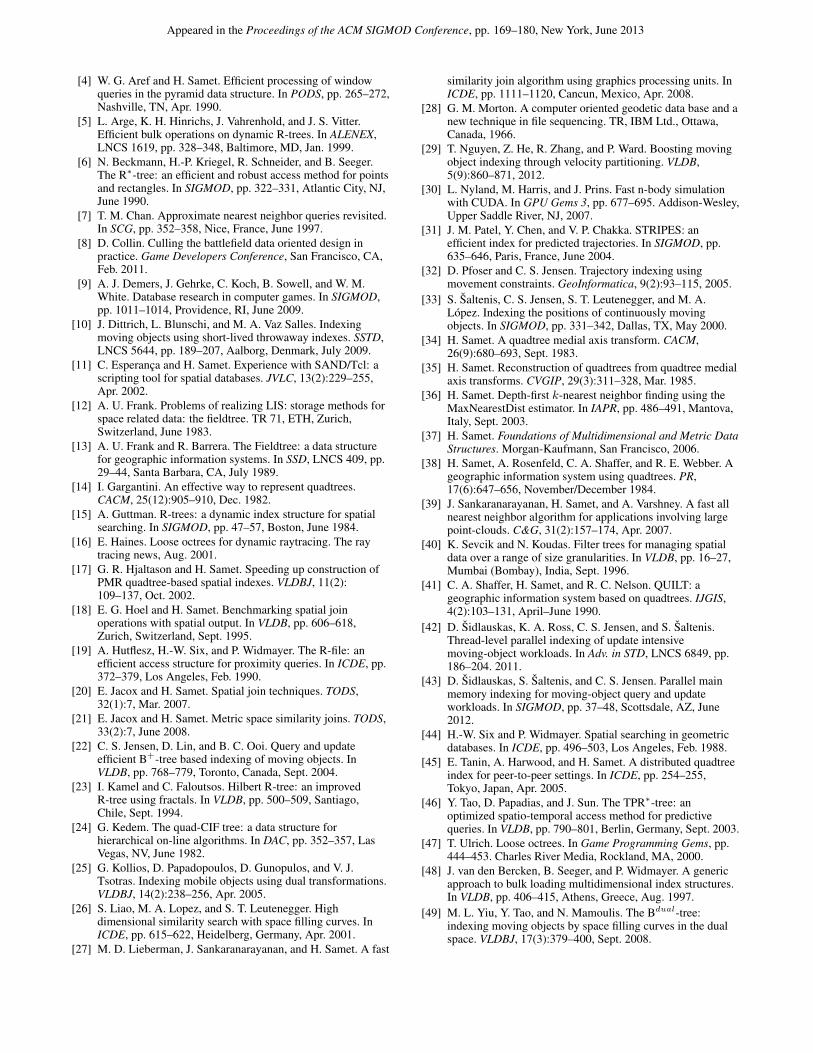
Notwithstanding the query performance of the loose quadtree, itis important to note that the act of updating objects constitutes themajority of the time of an N-body simulation, which is where theloose quadtree really excels. Figure 15 shows the update cost in-curred per frame due to the moving objects in the scene as well asthe time needed in milliseconds to render a frame using the loosequadtree with p = 0.999 and MX-CIF quadtree for varying sizesof the simulation. The performance of p = 1 is slightly worse thanp = 0.999 but better than the MX-CIF quadtree and is not shown inthe Figure. From the figure we see that the loose quadtree can ren-der frames 2–5 times faster than the MX-CIF quadtree. In partic-ular, even at 100,000 objects, the loose quadtree could still sustainabout 5 frames per second (210 milliseconds per frame) in contrastto the MX-CIF quadtree which at this size could not even render


43%

38%

31% 24%

39%

50

500

5000

RAY FRUS NN WIN-‐L WIN-‐S

Average Time in Nan

o Secs p = 1.0

p = 0.999 p = 0

(a)

1

10

100

1000

10000

RAY FRUS NN WIN-‐L WIN-‐S

Num

Blocks/Objects Examined

Blocks (p = 1.0) Blocks (p = 0.999) Blocks (p = 0) Objects (p = 1.0) Objects (p = 0.999) Objects (p = 0)

(b)

Figure 14: (a) Query times, using a log scale, for operations using the loose quadtree for values of p = 0 (theMX-CIF quadtree), p = 0.999, and p = 1 where p = 0.999 performs best as indicated with the percent improvementover the MX-CIF quadtree. (b) The average number of blocks and objects visited by the query

one frame per second (to be precise it took 1.4 seconds per frame).To put the size of the problem in a proper perspective, we note thatcurrent commercial games available in the market as of 2012 typi-cally do not involve more 15,000 thousand moving objects [8]. Inthis sense, we have shown that using loose quadtree makes it possi-ble to scale significantly these simulations vis-a-vis the state of theart. Furthermore, from Figure 15 we see that the time spent neededto update the underlying data structure using an MX-CIF quadtreeis at least 3 times more expensive when compared with the timeneeded when using a loose quadtree with p ≈ 1.

1

10

100

1000

10000

1

10

100

1000

10000

1 5 10 20 40 100

Upd

ate Time (M

illi-‐secon

ds)

Milli-‐S

econ

ds Per Frame (SPF)

Number of Objects in Simula>on in thousands

Time (p=0.999) Time (p=0) SPF (p=0.999) SPF (p=0)

Figure 15: Figure shows the milliseconds to render aframe and the time in milliseconds spent per frame toupdate the data structure for varying sizes of the simu-lations

7.3 R-treeWe have justified the use of the loose quadtree which permits

p to vary by comparing it with the MX-CIF quadtree which is aloose quadtree with p = 0. In order to provide an additional ref-erence point we also present a limited comparison with the R-treedata structure, described in Section 1, which is an object hierarchythat makes use of minimum bounding hypercube boxes somewhatin the same spirit as the MX-CIF quadtree except that the hierar-chies of different sets of objects are not in registration. We usedthe Hilbert R-tree [23] in our comparison as it is easy to construct.However, as expected, we found that updating the position of theobjects in the R-tree for each individual object was prohibitivelyexpensive, taking several orders of magnitude time more than theloose quadtree to perform the reinsertions upon execution of an up-date after a motion thereby making it practically unusable. There-fore, in order to improve the R-tree’s performance, we batched upall the objects that required reinsertion and then reinserted them asa single batch rather than one at a time. This approach was foundto be faster than rebuilding the structure from scratch. For the sim-

ulation with 14,000 objects, the update time for the R-tree structurewas 106.99 milliseconds per frame of the simulation. In compari-son, the update time for p = 0.999 was 22.11 milliseconds, whilefor the MX-CIF quadtree (i.e., p = 0), it was 82.26 milliseconds.So, our modified R-tree structure was still 25% worse than the MX-CIF quadtree but significantly worse (i.e., 5 times worse) than theloose quadtree with p = 0.999.

Next, we compared the query performance of the R-tree for thetwo window queries, WIN-L and WIN-S. Using the R-tree, the av-erage time to execute them was 167 nanoseconds for WIN-L and142 nanoseconds for WIN-S. In contrast, the query times of WIN-L and WIN-S were 128 and 113 nanoseconds, respectively, for theMX-CIF quadtree and 98 and 73 nanoseconds, respectively, forp = 0.999. These results show that the loose quadtree is supe-rior even when compared against an appropriately modified R-treevariant resulting in the loose quadtree being almost twice as fast.

8. CONCLUDING REMARKSWe have shown how to determine for a loose quadtree the

maximum possible width w of the minimum enclosing expandedquadtree cell c for an object o with MBHR(o,b,r) and cell expan-sion factor p. We have also shown that w is independent of the po-sition of o. This property enables determining the cell with whicho is associated and can be used, for example, in an algorithm tobuild a loose quadtree in an environment that deploys a pointer-less quadtree. In particular, this independence means that the algo-rithm requires little or no search and could be used, for example, topopulate a spatial database with the latest wave of multiprocessorssuch as those that make use of GPUs (e.g., [27]). It could also beused in point cloud applications (e.g., [39]). Our experiments (in-cluding the N-body simulation which did not rely on a pointerlessquadtree) have demonstrated that letting p take on a value infinites-imally smaller than 1 leads to the best results in minimizing theneed to update the index when objects are moving thereby increas-ing the size of the collection (i.e., database) of objects that can besupported. This is in contrast to the conventional use of p = 1 [47].

9. REFERENCES[1] D. J. Abel and J. L. Smith. A data structure and algorithm

based on a linear key for a rectangle retrieval problem.CVGIP, 24(1):1–13, Oct. 1983.

[2] D. J. Abel and J. L. Smith. A data structure and queryalgorithm for a database of areal entities. AustralianComputer Journal, 16(4):147–154, Nov. 1984.

[3] A. Aboulnaga and J. F. Naughton. Accurate estimation of thecost of spatial selections. In ICDE, pp. 123–134, San Diego,CA, Feb. 2000.


[4] W. G. Aref and H. Samet. Efficient processing of windowqueries in the pyramid data structure. In PODS, pp. 265–272,Nashville, TN, Apr. 1990.

[5] L. Arge, K. H. Hinrichs, J. Vahrenhold, and J. S. Vitter.Efficient bulk operations on dynamic R-trees. In ALENEX,LNCS 1619, pp. 328–348, Baltimore, MD, Jan. 1999.

[6] N. Beckmann, H.-P. Kriegel, R. Schneider, and B. Seeger.The R∗-tree: an efficient and robust access method for pointsand rectangles. In SIGMOD, pp. 322–331, Atlantic City, NJ,June 1990.

[7] T. M. Chan. Approximate nearest neighbor queries revisited.In SCG, pp. 352–358, Nice, France, June 1997.

[8] D. Collin. Culling the battlefield data oriented design inpractice. Game Developers Conference, San Francisco, CA,Feb. 2011.

[9] A. J. Demers, J. Gehrke, C. Koch, B. Sowell, and W. M.White. Database research in computer games. In SIGMOD,pp. 1011–1014, Providence, RI, June 2009.

[10] J. Dittrich, L. Blunschi, and M. A. Vaz Salles. Indexingmoving objects using short-lived throwaway indexes. SSTD,LNCS 5644, pp. 189–207, Aalborg, Denmark, July 2009.

[11] C. Esperança and H. Samet. Experience with SAND/Tcl: ascripting tool for spatial databases. JVLC, 13(2):229–255,Apr. 2002.

[12] A. U. Frank. Problems of realizing LIS: storage methods forspace related data: the fieldtree. TR 71, ETH, Zurich,Switzerland, June 1983.

[13] A. U. Frank and R. Barrera. The Fieldtree: a data structurefor geographic information systems. In SSD, LNCS 409, pp.29–44, Santa Barbara, CA, July 1989.

[14] I. Gargantini. An effective way to represent quadtrees.CACM, 25(12):905–910, Dec. 1982.

[15] A. Guttman. R-trees: a dynamic index structure for spatialsearching. In SIGMOD, pp. 47–57, Boston, June 1984.

[16] E. Haines. Loose octrees for dynamic raytracing. The raytracing news, Aug. 2001.

[17] G. R. Hjaltason and H. Samet. Speeding up construction ofPMR quadtree-based spatial indexes. VLDBJ, 11(2):109–137, Oct. 2002.

[18] E. G. Hoel and H. Samet. Benchmarking spatial joinoperations with spatial output. In VLDB, pp. 606–618,Zurich, Switzerland, Sept. 1995.

[19] A. Hutflesz, H.-W. Six, and P. Widmayer. The R-file: anefficient access structure for proximity queries. In ICDE, pp.372–379, Los Angeles, Feb. 1990.

[20] E. Jacox and H. Samet. Spatial join techniques. TODS,32(1):7, Mar. 2007.

[21] E. Jacox and H. Samet. Metric space similarity joins. TODS,33(2):7, June 2008.

[22] C. S. Jensen, D. Lin, and B. C. Ooi. Query and updateefficient B+-tree based indexing of moving objects. InVLDB, pp. 768–779, Toronto, Canada, Sept. 2004.

[23] I. Kamel and C. Faloutsos. Hilbert R-tree: an improvedR-tree using fractals. In VLDB, pp. 500–509, Santiago,Chile, Sept. 1994.

[24] G. Kedem. The quad-CIF tree: a data structure forhierarchical on-line algorithms. In DAC, pp. 352–357, LasVegas, NV, June 1982.

[25] G. Kollios, D. Papadopoulos, D. Gunopulos, and V. J.Tsotras. Indexing mobile objects using dual transformations.VLDBJ, 14(2):238–256, Apr. 2005.

[26] S. Liao, M. A. Lopez, and S. T. Leutenegger. Highdimensional similarity search with space filling curves. InICDE, pp. 615–622, Heidelberg, Germany, Apr. 2001.

[27] M. D. Lieberman, J. Sankaranarayanan, and H. Samet. A fast

similarity join algorithm using graphics processing units. InICDE, pp. 1111–1120, Cancun, Mexico, Apr. 2008.

[28] G. M. Morton. A computer oriented geodetic data base and anew technique in file sequencing. TR, IBM Ltd., Ottawa,Canada, 1966.

[29] T. Nguyen, Z. He, R. Zhang, and P. Ward. Boosting movingobject indexing through velocity partitioning. VLDB,5(9):860–871, 2012.

[30] L. Nyland, M. Harris, and J. Prins. Fast n-body simulationwith CUDA. In GPU Gems 3, pp. 677–695. Addison-Wesley,Upper Saddle River, NJ, 2007.

[31] J. M. Patel, Y. Chen, and V. P. Chakka. STRIPES: anefficient index for predicted trajectories. In SIGMOD, pp.635–646, Paris, France, June 2004.

[32] D. Pfoser and C. S. Jensen. Trajectory indexing usingmovement constraints. GeoInformatica, 9(2):93–115, 2005.

[33] S. Šaltenis, C. S. Jensen, S. T. Leutenegger, and M. A.López. Indexing the positions of continuously movingobjects. In SIGMOD, pp. 331–342, Dallas, TX, May 2000.

[34] H. Samet. A quadtree medial axis transform. CACM,26(9):680–693, Sept. 1983.

[35] H. Samet. Reconstruction of quadtrees from quadtree medialaxis transforms. CVGIP, 29(3):311–328, Mar. 1985.

[36] H. Samet. Depth-first k-nearest neighbor finding using theMaxNearestDist estimator. In IAPR, pp. 486–491, Mantova,Italy, Sept. 2003.

[37] H. Samet. Foundations of Multidimensional and Metric DataStructures. Morgan-Kaufmann, San Francisco, 2006.

[38] H. Samet, A. Rosenfeld, C. A. Shaffer, and R. E. Webber. Ageographic information system using quadtrees. PR,17(6):647–656, November/December 1984.

[39] J. Sankaranarayanan, H. Samet, and A. Varshney. A fast allnearest neighbor algorithm for applications involving largepoint-clouds. C&G, 31(2):157–174, Apr. 2007.

[40] K. Sevcik and N. Koudas. Filter trees for managing spatialdata over a range of size granularities. In VLDB, pp. 16–27,Mumbai (Bombay), India, Sept. 1996.

[41] C. A. Shaffer, H. Samet, and R. C. Nelson. QUILT: ageographic information system based on quadtrees. IJGIS,4(2):103–131, April–June 1990.

[42] D. Šidlauskas, K. A. Ross, C. S. Jensen, and S. Šaltenis.Thread-level parallel indexing of update intensivemoving-object workloads. In Adv. in STD, LNCS 6849, pp.186–204. 2011.

[43] D. Šidlauskas, S. Šaltenis, and C. S. Jensen. Parallel mainmemory indexing for moving-object query and updateworkloads. In SIGMOD, pp. 37–48, Scottsdale, AZ, June2012.

[44] H.-W. Six and P. Widmayer. Spatial searching in geometricdatabases. In ICDE, pp. 496–503, Los Angeles, Feb. 1988.

[45] E. Tanin, A. Harwood, and H. Samet. A distributed quadtreeindex for peer-to-peer settings. In ICDE, pp. 254–255,Tokyo, Japan, Apr. 2005.

[46] Y. Tao, D. Papadias, and J. Sun. The TPR∗-tree: anoptimized spatio-temporal access method for predictivequeries. In VLDB, pp. 790–801, Berlin, Germany, Sept. 2003.

[47] T. Ulrich. Loose octrees. In Game Programming Gems, pp.444–453. Charles River Media, Rockland, MA, 2000.

[48] J. van den Bercken, B. Seeger, and P. Widmayer. A genericapproach to bulk loading multidimensional index structures.In VLDB, pp. 406–415, Athens, Greece, Aug. 1997.

[49] M. L. Yiu, Y. Tao, and N. Mamoulis. The Bdual-tree:indexing moving objects by space filling curves in the dualspace. VLDBJ, 17(3):379–400, Sept. 2008.

indexing methods for moving object databases: games and other

Documents