increasing efficiency of line m123 through the …
TRANSCRIPT

i
INCREASING EFFICIENCY OF LINE M123
THROUGH THE APPLICATION OF TIME STUDY
AND LINE BALANCING METHOD
(CASE STUDY AT PT XY)
By
Muhammad Arif
ID No. 004201200023
A Thesis presented to the
Faculty of Engineering President University in partial
fulfillment of the requirements of Bachelor Degree in
Engineering Major in Industrial Engineering
2016
ii
THESIS ADVISOR
RECOMMENDATION LETTER
This thesis entitled “Increasing Efficiency of Line M123 Through the
Application of Time Study and Line Balancing Method (A case study in PT
XY)” prepared and submitted by Muhammad Arif in partial fulfillment of the
requirements for the degree of Bachelor Degree in the Faculty of Engineering has
been reviewed and found to have satisfied the requirements for a thesis fit to be
examined. I therefore recommend this thesis for Oral Defense.
Cikarang, Indonesia, January 28th
, 2016
Herwan Yusmira, Bsc. MET, MTech.

iii
DECLARATION OF ORIGINALITY
I declare that this thesis, entitled “Increasing Efficiency of Line M123 through
the Application of Time Study and Line Balancing Method (A case study in
PT XY)” is, to the best of my knowledge and belief, an original piece of work
that has not been submitted, either in whole or in part, to another university to
obtain a degree.
Cikarang, Indonesia, January 28th
, 2016
Muhammad Arif
iv
INCREASING EFFICIENCY OF LINE M123
THROUGH THE APPLICATION OF TIME STUDY
AND LINE BALANCING METHOD
(A case study in PT XY)
By
Muhammad Arif
ID No. 004201200023
Approved by
Herwan Yusmira, B.Sc. MET, MTech Ir. Andira, MT
Thesis Advisor 1 Thesis Advisor 2
Ir. Andira, MT
Program Head of Industrial Engineering

v
ABSTRACT
The focus of this research is to increase the line efficiency of line M123. The root
causes of having low efficiency itself are less accuracy and poor work
arrangement. Because of that, the output is not match the target and overtime must
be done. To overcome the problem, the root cause must be attacked by firstly
doing the time study prior the other method to be done. An accurate standard time
is expected to make the number of operator adequate and designing the work
arrangement smoothly without violating the takt time. To deal with a proper work
arrangement, line balancing method is used. The result shows that the efficiency
can be increased by 32.89% from previously 57.11% to 90%. The target output
can also be achieved together with the reduction number of operator. Thus, the
cost can be minimized.
Keywords: line efficiency, time study, standard time, line balancing, work
arrangement, cycle time, takt time

vi
ACKNOWLEDGEMENT
This thesis has never been done without my own effort and some supports from
people around me. Thus, I want to send my gratitude to Allah SWT for having
these guys around me.
1. Mom and Dad, thank you for all the things that you have given to me. I
would never run until this far without you in my life.
2. Kak Nova, kak Ira, and the Baby Sajid Ahnaf. You guys are one of my
reasons to keep me fighting for this thesis.
3. My lecturers, Mam Andira, Mam Anastasia, and Sir Herwan Yusmira.
Thank you for guiding me during my college life.
4. LSC department of PT XY, Cr, Mr K, Mr J, Ms B, Ms D, Ms DD, and Ms
A. Thanks for always surrounding myself with knowledge and cheers. You
guys contribute a lot in my life. Thanks for “Kaizen-ing” myself.
5. QA department of PT. MEAINA, thanks for accepting me in your
circumstances in my 1st Internship period.
6. Novando, Vero, Mr T and Mr R. Thanks for helping me finish this thesis.
7. Dudy, Fathur, Putera, Farhan, Aidil, Yoyo, and Rifi. I just feel you guys
are worth to be written here.
8. Generation of Eight (Genoit), there is none of my printed achievement
without the “Genoit” name in it.
9. Engineering 2012, thanks for the 3,5 years of togetherness and support.
vii
TABLE OF CONTENT
THESIS ADVISOR RECOMMENDATION LETTER ......................................... i
DECLARATION OF ORIGINALITY .................................................................. iii
LETTER OF APPROVAL ..................................................................................... iv
ABSTRACT ............................................................................................................ v
ACKNOWLEDGEMENT ..................................................................................... vi
TABLE OF CONTENT ........................................................................................ vii
LIST OF TABLE .................................................................................................... x
LIST OF FIGURES .............................................................................................. xii
LIST OF TERMINOLOGIES .............................................................................. xiii
CHAPTER I INTRODUCTION ............................ Error! Bookmark not defined.
1.1 Problem Background .................................... Error! Bookmark not defined.
1.2. Problem Statement ...................................... Error! Bookmark not defined.
1.3 Objectives ..................................................... Error! Bookmark not defined.
1.4 Scope ............................................................ Error! Bookmark not defined.
1.5 Assumption .................................................. Error! Bookmark not defined.
1.6 Research Outline .......................................... Error! Bookmark not defined.
CHAPTER II STUDY LITERATURE .................. Error! Bookmark not defined.
2.1. Time study ................................................... Error! Bookmark not defined.
2.1.1 Rating Performance ............................... Error! Bookmark not defined.
2.1.2 Normal Time ......................................... Error! Bookmark not defined.
2.1.3 Allowance ............................................. Error! Bookmark not defined.
2.1.4 Standard Time ....................................... Error! Bookmark not defined.
2.2 Data Validity Testing ................................... Error! Bookmark not defined.
2.2.1 Normality Test ...................................... Error! Bookmark not defined.
2.2.2 Uniformity Test ..................................... Error! Bookmark not defined.
2.2.3 Sufficiency Test .................................... Error! Bookmark not defined.
2.3 Operation Process Chart ............................... Error! Bookmark not defined.
2.4 Line Balancing ............................................. Error! Bookmark not defined.
2.4.1 Methods of Line Balancing ................... Error! Bookmark not defined.
2.4.2 Measurement of Line Balancing ........... Error! Bookmark not defined.
CHAPTER III RESEARCH METHODOLOGY .. Error! Bookmark not defined.

viii
3.1 Initial Observation ........................................ Error! Bookmark not defined.
3.2 Problem Identification .................................. Error! Bookmark not defined.
3.3 Literature Study ............................................ Error! Bookmark not defined.
3.4 Data Collection and Analysis ....................... Error! Bookmark not defined.
3.4.1 Data Collection...................................... Error! Bookmark not defined.
3.4.2 Data Analysis ........................................ Error! Bookmark not defined.
3.5 Application of Line Balancing Method ....... Error! Bookmark not defined.
3.6 Conclusion and Recommendation................ Error! Bookmark not defined.
3.7 Research Framework .................................... Error! Bookmark not defined.
CHAPTER IV DATA COLLECTION AND ANALYSISError! Bookmark not
defined.
4.1 Initial Line Efficiency .................................. Error! Bookmark not defined.
4.2 Analyzing Root Cause of Low Efficiency ... Error! Bookmark not defined.
4.2.1 Observing the Standard Determined by CompanyError! Bookmark
not defined.
4.2.3 Number of Operator .............................. Error! Bookmark not defined.
4.3 Standard Time at M123 ................................ Error! Bookmark not defined.
4.4 Standard Time before Time Study ............... Error! Bookmark not defined.
4.5 Actual Standard Time .................................. Error! Bookmark not defined.
4.5.1 Normality Test ...................................... Error! Bookmark not defined.
4.5.2 Uniformity Test ..................................... Error! Bookmark not defined.
4.5.3 Sufficiency Test .................................... Error! Bookmark not defined.
4.5.4 Performance Rating ............................... Error! Bookmark not defined.
4.5.5 Normal Time ......................................... Error! Bookmark not defined.
4.5.6 PFD (Personal, Fatigue, and Delay) ...... Error! Bookmark not defined.
4.5.7 Standard Time ....................................... Error! Bookmark not defined.
4.6 Line Balancing ............................................. Error! Bookmark not defined.
4.6.1 Largest Candidate Rule ......................... Error! Bookmark not defined.
4.6.2 Killbridge and Wester Method .............. Error! Bookmark not defined.
4.6.3 Rank Positional Weight ........................ Error! Bookmark not defined.
4.7 Comparison of Three Methods..................... Error! Bookmark not defined.
4.7.1 Balance Delay ....................................... Error! Bookmark not defined.
4.8 Additional Action ......................................... Error! Bookmark not defined.
4.9 Final Evaluation ........................................... Error! Bookmark not defined.

ix
4.9 Comparison of Current and Proposed Line .. Error! Bookmark not defined.
CHAPTER V CONCLUSION AND RECOMMENDATIONError! Bookmark
not defined.
5.1 Conclusion ............................................... Error! Bookmark not defined.
5.2 Recommendation ..................................... Error! Bookmark not defined.
REFERENCES ....................................................... Error! Bookmark not defined.
APPENDICES ....................................................... Error! Bookmark not defined.
Appendix 1 OPC Before ........................................ Error! Bookmark not defined.
Appendix 2 OPC After ........................................... Error! Bookmark not defined.
Appendix 3 Criteria of Skill and Effort ................. Error! Bookmark not defined.
Appendix 4 Performance Rating Calculation ........ Error! Bookmark not defined.
Appendix 5 Result of Time Study ......................... Error! Bookmark not defined.
Appendix 6 Sufficiency Test .................................. Error! Bookmark not defined.
Appendix 7 Comparison Table between the before and after observation .... Error!
Bookmark not defined.
Appendix 8 Rank Position Weight Matrix ............. Error! Bookmark not defined.
Appendix 9 Supporting Tools ................................ Error! Bookmark not defined.
x
LIST OF TABLE
Table 2. 1 Performance Rating .............................. Error! Bookmark not defined.
Table 2. 2 Effort Rating ......................................... Error! Bookmark not defined.
Table 2. 3 Condition Rating ................................... Error! Bookmark not defined.
Table 2. 4 Consistency Rating ............................... Error! Bookmark not defined.
Table 2. 5 Performance Rating Calculation ........... Error! Bookmark not defined.
Table 2. 6 Largest Candidate Rule Table Example Error! Bookmark not defined.
Table 2. 7 Table of Task Assigned Using LCR MethodError! Bookmark not
defined.
Table 2. 8 Killbridge and Wester's Method ExampleError! Bookmark not
defined.
Table 2. 9 Determined Work Station ..................... Error! Bookmark not defined.
Table 2. 10 Ranked Positon Weight Method ......... Error! Bookmark not defined.
Table 2. 11 Determined Work Station ................... Error! Bookmark not defined.
Table 4.1 Current Line Efficiency ......................... Error! Bookmark not defined.
Table 4. 2 Standard time before time study ........... Error! Bookmark not defined.
Table 4. 3 Performance of Operator 1 .................... Error! Bookmark not defined.
Table 4. 4 Actual Standard Time ........................... Error! Bookmark not defined.
Table 4. 5 Precedence Table .................................. Error! Bookmark not defined.
Table 4. 6 Precedence Table (continued) ............... Error! Bookmark not defined.
Table 4. 7 Proposed Work Station ......................... Error! Bookmark not defined.
Table 4. 8 Evaluation of LCR ................................ Error! Bookmark not defined.
Table 4. 9 Killbridge and Wester Method .............. Error! Bookmark not defined.
Table 4. 10 Evaluation of KWM ............................ Error! Bookmark not defined.
Table 4. 11 Work Station of RPW Application ..... Error! Bookmark not defined.
Table 4. 12 Smoothness Index of RPW ................. Error! Bookmark not defined.
Table 4. 13 Cycle time of attaching head ............... Error! Bookmark not defined.
Table 4. 14 New cycle time of work station 14 ..... Error! Bookmark not defined.
Table 4. 15 New cycle time for work station 17 .... Error! Bookmark not defined.
Table 4. 16 New cycle time for work station 16 .... Error! Bookmark not defined.
Table 4. 17 New cycle time for work station 22 .... Error! Bookmark not defined.

xi
Table 4. 18 New cycle time for work station 3 ...... Error! Bookmark not defined.
Table 4. 19 New cycle time for work station 4 ...... Error! Bookmark not defined.
Table 4. 20 New cycle time for work station 9 ...... Error! Bookmark not defined.
Table 4. 21 New cycle time for each work station . Error! Bookmark not defined.
Table 4. 22 Evaluation of Final Work ArrangementError! Bookmark not
defined.
Table 4. 23 The result of improvement .................. Error! Bookmark not defined.
Table 4. 24 Cost comparison between actual and after improvement condition
................................................................................ Error! Bookmark not defined.

xii
LIST OF FIGURES
Figure 2. 1 Example of Operation Process Chart ... Error! Bookmark not defined.
Figure 2. 2 Precedence Diagram ............................ Error! Bookmark not defined.
Figure 2. 3 Work Station Determined Using KWM MethodError! Bookmark not
defined.
Figure 2. 4 Precedence Diagram ............................ Error! Bookmark not defined.
Figure 2. 5 Determined Work Station .................... Error! Bookmark not defined.
Figure 3. 1 Research Flow ..................................... Error! Bookmark not defined.
Figure 3. 2 Research Framework ........................... Error! Bookmark not defined.
Figure 4. 1 Fishbone Diagram of Root Cause AnalysisError! Bookmark not
defined.
Figure 4. 2 Yamazumi of Labor Data Sheet .......... Error! Bookmark not defined.
Figure 4. 3 Actual time vs LDS time ..................... Error! Bookmark not defined.
Figure 4. 4 Precedence Diagram ............................ Error! Bookmark not defined.
Figure 4. 5 Yamazumi Chart of LCR Method ApplicationError! Bookmark not
defined.
Figure 4. 6 Proposed Layout of Largest Candidate RuleError! Bookmark not
defined.
Figure 4. 7 Killbridge and Wester Method ............ Error! Bookmark not defined.
Figure 4. 8 Yamazumi Chart of KWM .................. Error! Bookmark not defined.
Figure 4. 9 Yamazumi Chart of RPW method applicationError! Bookmark not
defined.
Figure 4. 10 Proposed Layout of Rank Position WeightError! Bookmark not
defined.
Figure 4. 11 Balance Delay Comparison ............... Error! Bookmark not defined.
Figure 4. 12 Efficiency Comparison ...................... Error! Bookmark not defined.
Figure 4. 13 Smoothness Index Comparison ......... Error! Bookmark not defined.
Figure 4. 14 Chosen Yamazumi Chart of RPW ApplicationError! Bookmark not
defined.
Figure 4. 15 Improved Yamazumi Chart ............... Error! Bookmark not defined.

xiii
Figure 4. 16 Comparison between current and proposed lineError! Bookmark
not defined.

xiv
LIST OF TERMINOLOGIES
Efficiency : the comparison of what is actually produced with
what can be achieved with the same consumption of
resources
Line balancing : the process of assigning tasks to workstations in such
a way that the workstation have approximately equal
time requirement
Balance delay : the amount of idle on production assembly lines
caused by the uneven division of work among
operators and stations
LDS : Labor Data Sheet; a data that gives information
about the target output, takt time, number of
operators, and work arrangement
Cycle time : the period required to complete one cycle of an
operation, or to complete a function, job, or task
from start to finish
Lead time : the amount of time between the placing of an order
and the receipt of the goods ordered
Normal time : the amount of time required for a repeated operation
by an experienced worker of average skill working at
a normal pace
OPC : Operation Process Chart ; a graphical representation
of the sequence of steps constituting a process, from
raw materials through to the finished product
Performance rating : a process to evaluate the performance of the
operators
Precedence diagram : a visual representation techniques that depicts the
activities involved in a project and the dependencies
among those activities

xv
Significance level : the probability that the test will reject null hypothesis
when the hypothesis is true
Smoothness index : a scale that shows the extent level of smoothness of
the production line
Standard time : the time for completing the work process with
allowance
Takt time : the amount of time necessary to build one unit to
satisfy customer demand
Time study : the examination and analysis of time and motion
required to complete an action
Yamazumi chart : a stacked bar chart that shows the balance of cycle
time workloads between a number of operators
typically in an assembly line or work cell

16

ABSTRACT
The focus of this research is to increase the line efficiency of line M123. The root
causes of having low efficiency itself are less accuracy and poor work
arrangement. Because of that, the output is not match the target and overtime must
be done. To overcome the problem, the root cause must be attacked by firstly
doing the time study prior the other method to be done. An accurate standard time
is expected to make the number of operator adequate and designing the work
arrangement smoothly without violating the takt time. To deal with a proper work
arrangement, line balancing method is used. The result shows that the efficiency
can be increased by 32.89% from previously 57.11% to 90%. The target output
can also be achieved together with the reduction number of operator. Thus, the
cost can be minimized.
Keywords: line efficiency, time study, standard time, line balancing, work
arrangement, cycle time, takt time
CHAPTER I
INTRODUCTION
1.1 Problem Background
Efficiency is something essential for a company especially for the company
running a mass production business and utilizes much kind of resources. Having a
good efficiency will be very beneficial. High efficiency means all the resources
such as human, material, space, and machines are well utilized. There is no excess
and the waste is minimized. By having such these things, the cost can
automatically be properly-allocated and minimized. These benefits can strength
the position of the company in the business competition. Producing maximal
output with a short lead time and fulfilling the demand of customers are
something that every company has dreamt of.
PT XY that will be called PT XY for the next is one of multinational company in
Indonesia. This company is one of the biggest toy manufacturing in the world.
The main focus of the company’s activities is producing dolls. The dolls
manufactured are mainly distributed to America and Europe continent. These two
continents give a very big impact to the sales rating especially when Halloween
and Christmas. These two occasions are the condition where people usually tend
to give present. This is the main consideration of head quarter in determining the
order number that must be fulfilled by PT XY.
A good efficiency is very important for PT XY as the subsidiary. PT XY must be
able to manage the resource well in order to fulfill the demand given by
headquarter. The demand will be very high at certain period. In this case, of
course the head quarter do not want to lose the opportunity and will ask PT XY to
deliver the product at the very right time. This will help PT XY in minimizing
cost for the excessive stuff such as inventory, labor, and machine utilization. That
is why efficiency is way very important for PT XY.

There are three major process in manufacturing the dolls; primary process, sewing
process, and secondary process. The primary process is the process where basic
part of dolls is made such as torso. Primary process also includes the rooting
process. Sewing process includes costume development and costume sewing
production. The last is secondary process which is also called final assembly
process where the dolls and its accessories are packed. Those are the three major
processes at PT XY.
As one of leading doll manufacturing company, PT XY has always targeted a high
standard for efficiency. Thus, every production line at PT XY is automatically
expected to have good efficiency. Last year, the efficiency target of PT XY was
81%. This year, the company levels the efficiency up to 90%. It means that every
production line at PT XY should have minimum efficiency of 90% to support the
company’s goal.
The fact, some of the production lines at PT XY still have line efficiency below
90% especially at line M123. At week ending 10/12/2015, the line efficiency
touches the number of 57%. It is way far from the target established by the
company and it cost for excess or shortages. Based on the efficiency target, this
production line does not fulfill the standard established by PT XY. Looking at this
problem, thus it is needed to increase the line efficiency since the demand can
sometimes be very high for several products. Through this thesis, it is expected
that line production can achieve the efficiency target set by PT XY.
1.2. Problem Statement
Based on the background explanation above, several problem statements can be
conducted:
What is the root cause of low efficiency at line M123?
How to increase the line efficiency at line M123?
1.3 Objectives
There is an objective to be achieved through this research

To improve efficiency of line M123
1.4 Scope
Due to the limitation of resources, the scope of this research will be limited:
Head Count Addition or Head Count Elimination can only be done by
secondary area management
The observation is done from October 12th
– October 15th
2015
1.5 Assumption
Assumptions must be made in this research to create an appropriate model.
The skill of operators are assumed to be the equally-likely
The target of output is equal during observation
Material are always available during production process
1.6 Research Outline
Chapter I Introduction
This chapter includes the problem background,
research questions, objectives, scope and limitation of
the research as well as the research outline.
Chapter II Study Literature
This chapter includes study time study, line balancing,
and other tools that can support this final project.
Chapter III Research Methodology
All systematic steps and detailed framework are
provided in this chapter to arrange this research to be
conducted methodically. The framework is made
regarding the literature study as well.
Chapter IV Data Analysis
The data that have been collected will be analyzed
through this chapter. The main result will be the new
arrangement of the work station that is expected to
increase efficiency.
Chapter V Conclusion and Recommendation
This chapter includes the summary of the research
together with the recommendation for the future
research.
Through this chapter, the problem and objectives of the research have been
clearly-stated together with the scope and assumptions. Thus, this research has
gotten its direction in the process of achieving the objectives. To meet the
objectives, it needs also to find a way to solve the problem. Therefore, some
literature about related subject will be delivered in the next chapter.

CHAPTER II
STUDY LITERATURE
2.1. Time study
It is important to tally the real time to complete procedures in the generation line.
This should be possible by utilizing an instrument, for example, stopwatch. Along
these lines it is called stopwatch time study. There are two systems in working
with this stopwatch, back to back timing technique and snapback strategy. While
persistent timing strategy permits the stopwatch to keep running for the whole
span of study, snapback system breaks the procedure into components. Sometime
study investigator use both routines, trusting that 9 studies dominatingly long
components are more versatile to snapback readings, while short cycle studies are
more qualified to the nonstop strategy (Niebel, 2003).
At the point when parts of time study contains a wide differing qualities of
systems to focus the measure of time needed, under an astounding estimation of
the state, for work related with the human, machine, or a mix of both. It is has
been presented by Frederick W. Taylor since the year 1881, yet is still generally
utilized as a technique for time study. For the most part, time study is utilized to
gauge work. The choice results than the time study is the period in which an
individual as per work or errand and completely prepared to use particular system,
will perform this errand if the specialist in the typical or master. This is known as
the time standard for operation. Adjust the master for a work may be made
through a few routines, where every Method is utilized just as per some particular
circumstances. Time study is incorporate utilizing stopwatch, 'Foreordained
Motion Time System or Synthetic Time System', and 'Work or Action Sampling".
On the other hand, in this study, just the time study utilizing Stopwatch Time
Study will be utilized as a part of the time estimation. The time study was
additionally permitted to deduct all visitors. Institutionalization is the target to be
accomplished. These insights may be demonstrated by the work inspecting
operation. On the off chance that standard set, execution enhanced to normal 85%.
This is a 42% increment in execution.
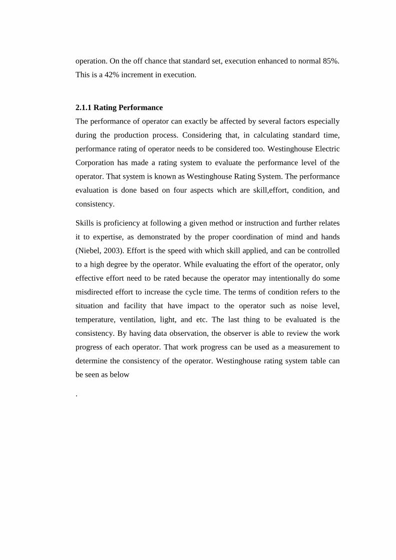
2.1.1 Rating Performance
The performance of operator can exactly be affected by several factors especially
during the production process. Considering that, in calculating standard time,
performance rating of operator needs to be considered too. Westinghouse Electric
Corporation has made a rating system to evaluate the performance level of the
operator. That system is known as Westinghouse Rating System. The performance
evaluation is done based on four aspects which are skill,effort, condition, and
consistency.
Skills is proficiency at following a given method or instruction and further relates
it to expertise, as demonstrated by the proper coordination of mind and hands
(Niebel, 2003). Effort is the speed with which skill applied, and can be controlled
to a high degree by the operator. While evaluating the effort of the operator, only
effective effort need to be rated because the operator may intentionally do some
misdirected effort to increase the cycle time. The terms of condition refers to the
situation and facility that have impact to the operator such as noise level,
temperature, ventilation, light, and etc. The last thing to be evaluated is the
consistency. By having data observation, the observer is able to review the work
progress of each operator. That work progress can be used as a measurement to
determine the consistency of the operator. Westinghouse rating system table can
be seen as below
.

Table 2. 1 Performance Rating
Table 2. 2 Effort Rating
+0.13 A1 Excessive
+0.12 A2 Excessive
+0.1 B1 Excellent
+0.08 B2 Excellent
+0.05 C1 Good
+0.02 C2 Good
0 D Average
-0.04 E1 Fair
-0.08 E2 Fair
-0.12 F1 Poor
-0.17 F2 Poor
Table 2. 3 Condition Rating
+0.06 A Ideal
+0.04 B Excellent
+0.02 C Good
0 D Average
-0.03 E Fair
-0.07 F Poor
+0.15 A1 Superskill
+0.13 A2 Superskill
+0.11 B1 Excellent
+0.08 B2 Excellent
+0.06 C1 Good
+0.03 C2 Good
0 D Average
-0.05 E1 Fair
-0.1 E2 Fair
-0.16 F1 Poor
-0.22 F2 Poor

Table 2. 4 Consistency Rating
+0.04 A Perfect
+0.03 B Excellent
+0.01 C Good
0 D Average
-0.02 E Fair
-0.04 F Poor
Karger (1977) provides the criteria of skill and effort. The criteria provided are
able to help the operators to rate the operators. For more detail, it can be seen on
appendices.
After finishing the performance evaluation, the ratings from those factors can be
summed up. For more detail, the table below provides the example of calculation
for the performance factor. The result of this calculation
Table 2. 5 Performance Rating Calculation
Skill C2 +0.03
Effort C1 +0.05
Condition D +0.00
Consistency E -0.02
Algebraic Sum +0.06
Performance Rating 1.06
Some companies have modified the application of Westinghouse system. Some
thought stated that in certain condition, the value can be rated as zero value. It
means there is no impact to the performance of operators. While consistency is
related to skills, thus the value of consistency is no longer counted. Therefore,
conditions and consistency are omitted as the factors in determining the
performance rating.
2.1.2 Normal Time
Normal time is the measure of time needed for a repeated operation by a trained
worker of normal expertise working at an ordinary pace. It is come about because

(2-1)
(2-2)
of the augmentation between watched time and execution rating of the operator
(Niebel, 2003).
2.1.3 Allowance
Fundamentally, allowance is divided into three classes which are constant
allowance, variable allowance, and special allowance. Constant allowance can be
defined as the time dealt by operator to take care of personal needs. This basic
allowance is an initial allowance for operator. Except the personal issues, the
operator may have another issue from external factors that will affect the
performance of operator. This tolerance is covered by variable fatigue allowance.
Special allowance is the tolerance time to deal with external factors that have no
impact to the operator but to the operation such as to the equipment and material.
Those are the categories of allowance.
2.1.4 Standard Time
After calculating the PFD (Personal, Fatigue, and Delay) allowance, the standard
time can be established. The term of standard time is the time needed for a
completely qualified, prepared operator, working at standard pace and applying
normal exertion, to perform the operation (Niebel, 2003).
2.2 Data Validity Testing
2.2.1 Normality Test
It is important to know whether the data is normally distribute or not, meaning
that the statistical inference must be determined. There are two options in creating
statistical inference; they are confidence interval or hypothesis testing. In
confidence interval, it means that the population is unknown (Hayter, 2000).

(2-4)
(2-3)
There are some equation can be utilized to focus the ordinariness of an
arrangement of information, one of them is by utilizing p-esteem. The speculation
comprises of two announcements, invalid theory (H0) and option theory (HA).
Invalid speculation is an announcement of a zero or invalid contrast that is
straightforwardly tried. This will relate to the first claim if that claim incorporates
the state of no change (=) or contrast, for example, ≥ or ≤. Invalid speculation is
tried straightforwardly since the last conclusion will be either dismissal of H0 or
inability to dismiss H0 (Walpole, 2002). On the off chance that H0 is rejected,
then HA must be valid.
With a specific end goal to check the typicality of the dissemination, the null
hypothesis (H0) and alternative hypothesis (HA) must be expressed as underneath
H0: The data is normally distributed
HA: The data is not normally distributed
2.2.2 Uniformity Test
Beside the normality, uniformity of data must also be checked. One collection of
data can pass the normality test but sometimes the variance is too big. Thus, the
data is significantly different between one and another. Then, the limit must be
created through this test to ensure the separation is still in the desired level. If it is
out of the control limit, then the out-of-limit data must be omitted. This is the step
to determine the uniformity of data:
a. Calculate average observed time (x) for each operation
b. Calculate the standard deviation (s) of each operation (Wignjosoebroto, 2000).

(2-5)
(2-6)
c. Focus the Upper Control Limit (UCL) and Lower Control Limit (LCL)
(Wignjosoebroto, 2000). This point of confinement will decide how uniform
the information each other. The littler the farthest point, the more the
information will be uniform. More than 99% of the region under any typical
dispersion is encased in the reach that known as six sigma limits (Taha, 1987).
The following is the recipe to focus UCL and LCL in six sigma limits.
2.2.3 Sufficiency Test
The purpose of sufficiency test is to find how much observation needed to reach
the confidence level. Thus, the more the variance of data, the more observation
needed. The following formula can calculate how much observation needed to
achieve 95% confidence level (Sutalaksana, 2006). N’ is the number observation
that must be done. The data is considered enough when n (number of data) is
bigger than N’.
2.3 Operation Process Chart
Operation process chart is a diagram depicting the steps of assembling material,
started from raw material until component or finished product. Operation process
chart contain information for further analysis.
Time wasted, material used, and the space or machine utilized for material
processing. So, in one complete Operation Process Chart, the recorded processes
are operation and inspection, storing will sometimes be put at the end of the
process.
For more complete comprehension of Operation Process Chart, the following
figure is the complete process of telephone manufacturing starting from the
assembling the component until the final inspection of finished product.

Source: Niebel's Methods, Standards, and Work Design 12th Edition
Figure 2. 1 Example of Operation Process Chart

2.4 Line Balancing
2.4.1 Methods of Line Balancing
Line balancing means balancing the production lines or assembly lines. The
principle goal of line balancing is to set the assignment uniformly over the work
station with the goal that sit without wasted time of man or machine can be
minimized. Line balancing goes for gathering the laborers in an effective example
with a specific end goal to get an ideal or most effective equalization of the
capacities and the flow of the process or assembly process.
Line balancing is also known as a term to process of determining the tasks in a
work stations in a production sequences. The tasks itself consist of the necessary
operations to convert the raw material to finished goods. Line balancing is a
classic operation of optimization technique having a very significant effect to
industries especially in applying the lean concept. The principle of mass
production is involving line balancing of assembling the similar components or
changing components in different production level of work station. As the
knowledge about line balancing is getting better, perfection and in line balancing
procedure is being continuously developed and it is a must for the sake of
industries. The proficient work allocation is purposed to achieve a good efficiency
and productivity.
There are several method used to balance the production lines. Three method of
line balancing will be explained through this literature study. The methods are
Largest Candidate Rule (LCR), Killbridge and Wester’s Method (KWM), and
Ranked Positional Weight Method (RPW).
2.4.1.1 Largest Candidate Rule (LCR) Method
It is known that the main purpose of line balancing is to distribute the total
workload evenly and smoothly although in fact, it is impossible to achieve the
perfect balancing among workers. This is the role of line balancing efficiency
related to differences in minimum rational work element time and the precedence
constraints between the elements. Largest Candidate Rule method arranges the
work element in a descending order (referred to the work station and work

element) for each work station and not exceeding the allowable precedence.
Below is the example of Largest Candidate Rule Application in balancing the line.
Table 2. 6 Largest Candidate Rule Table Example
Source: Line Balancing Using Largest Candidate Rule Algorithm in a Garment Industry
An assignment should be possible by machines of diverse sorts furthermore by
administrators of distinctive work sorts. The handling time of any errand is a
variable controlled by the expertise level also, productivity of the administrator.
The work is isolated in a manner that every administrator gets equivalent work
load. The applied system proposed and quickly abridged in the going before
segment fills the need of exhibiting how the proposed system would work. Table
above portrays the work components organized by. At that point figure above
demonstrates the Operator line adjusting graph after the line adjusting procedure
and the administrator process durations have been expanded by giving the laborers
additional operations and the unmoving times of the specialists was decreased and
to enhance the productivity. Thus the operation was handled by 16 workers is just
reduced by 50 % to 8 workers. Line balancing Efficiency (to be) = 85.5%

Table 2. 7 Table of Task Assigned Using LCR Method
Source: Line Balancing Using Largest Candidate Rule Algorithm in a Garment Industry
Above is the table of arrangement of the workstation after the balancing process
based on the Largest Candidate Rule (LCR) method.
2.4.1.2 Killbridge and Wester’s Method (KWM) Method
Kilbridge and Wester (segment) system is a heuristic method that chooses work
components for task to stations as indicated by their positions in the precedence
diagram. This techniques known for its unwavering quality in conquering the
troubles, for example, experienced in Largest Candidates Rule system where a
component could be chosen as for high Te Value however independent of its

position in the priority outline. However in the section technique the components
are arranged into columns.
Table 2. 8 Killbridge and Wester's Method Example
Source: Selection of Balancing Method for Manual Assembly Line of Two Stages Gearbox
Above is the example of Killbridge and Wester’s method example. It includes the
work element of the lines together with its cycle time for each work element.
There will also the determination of column for each work element. The
precedence of each work element must be put there on the table.
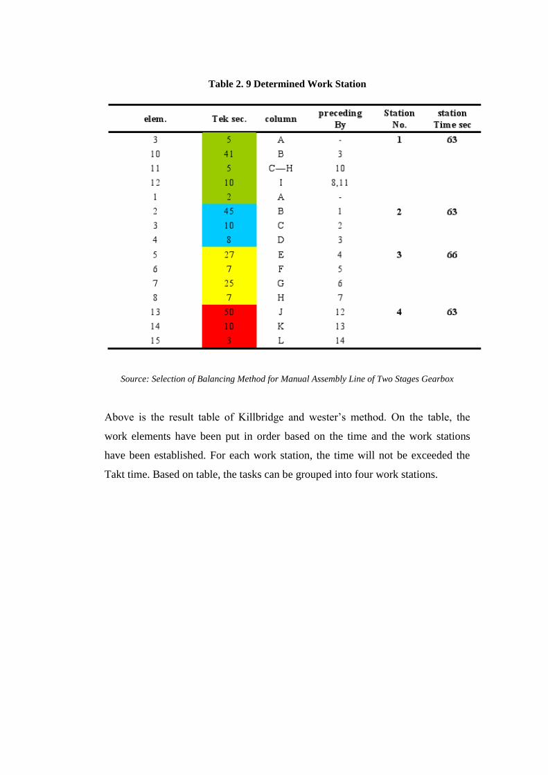
Table 2. 9 Determined Work Station
Source: Selection of Balancing Method for Manual Assembly Line of Two Stages Gearbox
Above is the result table of Killbridge and wester’s method. On the table, the
work elements have been put in order based on the time and the work stations
have been established. For each work station, the time will not be exceeded the
Takt time. Based on table, the tasks can be grouped into four work stations.

Figure 2. 2 Precedence Diagram
Source: Selection of Balancing Method for Manual Assembly Line of Two Stages Gearbox
Figure 2. 3 Work Station Determined Using KWM Method
Source: Selection of Balancing Method for Manual Assembly Line of Two Stages Gearbox
2.4.1.3 Ranked Positional Weight Method
Ranked Positional Weight method is used to calculate for each element. The
method accounted the Takt time value and the position at the precedence diagram.
RPW is computed by summing Takt time and other time for the element that
follow the takt time in the arrow of precedence diagram. Then, the time is

rearranged using the previous step. The work element can be seen at the table
below and the table can also be generated using RPW table. The idle time was set
to be 0 second for Station 2 with 1, 5 and 3 seconds for stations 1, 3 and 4 as it is
on the figure below. In this case, Station 2 is the bottleneck station.
Figure 2. 4 Precedence Diagram
Source: Selection of Balancing Method for Manual Assembly Line of Two Stages Gearbox
Above is the example of precedence diagram in one sequence of production for an
assembly line. Each of the work elements is preceded by some or one work
elements. Then, it should be made in sequence to make it order and easier to work
stationing process.
Figure 2. 5 Determined Work Station
Source: Selection of Balancing Method for Manual Assembly Line of Two Stages Gearbox

Above is the output after balancing the process using the Ranked Positional
Weight method. The result of the method state that the tasks can be grouped in to
four stations. Each station consists of some tasks that can be done by one operator.
Table 2. 10 Ranked Positon Weight Method

Table 2. 11 Determined Work Station
Source: Selection of Balancing Method for Manual Assembly Line of Two Stages Gearbox
The tables above are the sequence of the operation that is put on the tables. The
first table above shows the precedence task of another task together with the
weighted value for each work element. The takt time is also put there.
After determining the table of precedence and takt time, then the next step is
making the table consist of the established work station based on the Ranked
Positional Weight Method.
2.4.2 Measurement of Line Balancing
2.4.2.1 Takt Time
Takt time is characterized as the measure of time important to fabricate one unit to
fulfill client interest (Till, 2010). Each procedure must be finished in under takt
time unless the yield of creation won't meet the arranging calendar. Net accessible
time and every day request must be resolved before computing takt time. Net
accessible time is the measure of time accessible for work to be finished. This

(2-7)
(2-8)
(2-9)
rejects break times and any normal stoppage time, for example, planned support,
group briefings, and meal break. Takt time is characterized by this equation below
2.4.2.2 Yamazumi Chart
A Yamazumi outline is a stacked bar graph that demonstrates the parity of process
duration workloads between various administrators regularly in mechanical
production system or work cell (Minkjan, 2009). This graph will likewise
distinguish whether any procedure surpass takt time or not. In this way, the
quantity of yield every day could likewise be anticipated.
2.4.2.3 Number of Operator
In the wake of figuring the standard time, the measure of operator number must be
chosen (Elsayed, 1985).
Where:
Ti = time from process 1-k
Tt = takt time
2.4.2.4 Line Efficiency
PT XY characterizes the line efficiency as the correlation between end hours and
accessible/available hours. The standard time in the estimation is the standard
time in producing 1,000 yields.
(2-10)
(2-11)
(2-12)
(2-13)
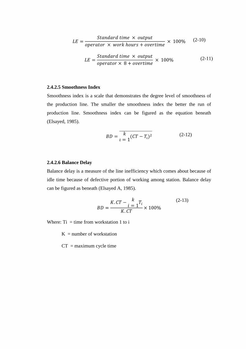
2.4.2.5 Smoothness Index
Smoothness index is a scale that demonstrates the degree level of smoothness of
the production line. The smaller the smoothness index the better the run of
production line. Smoothness index can be figured as the equation beneath
(Elsayed, 1985).
2.4.2.6 Balance Delay
Balance delay is a measure of the line inefficiency which comes about because of
idle time because of defective portion of working among station. Balance delay
can be figured as beneath (Elsayed A, 1985).
Where: Ti = time from workstation 1 to i
K = number of workstation
CT = maximum cycle time
CHAPTER III
RESEARCH METHODOLOGY
This Chapter informs the reader how the research was conducted by describing
the detail steps in conducting the research. The steps should be set systematically
to help the researcher solve the initial problems. By constructing the suitable
research methodology, the research and analysis can be done accurately. Hereby
the steps performed to solve the initial problems in this research are on figure 3.1
Initial
Observation
Problem
Identification
Literature Study
Initial Observation
To understand the current condition of efficiency
at PT. XY
To observe and understand the condition of line
M123
To observe the current balancing method
Problem Identification
To identify the effect of having low efficiency
while the efficiency target is high
To define the objective of research
To define the scope, limitations, and assumptions
used in the research
Literature Study
To explain the definition of time study, line
balancing and simulation
To determine the method problem solving
To describe how the method will be used
3.1 Initial Observation
The initial observation is meant as the first step to begin the research. This step is
purposed to deeply know the current condition at PT XY especially the line
efficiency condition and the existing task distribution at each line. It is also
purposed to see how the current method used to balance the line at PT XY. The
problem going to be discussed will be related to those things above as the focus of
this research is to increase the line efficiency of the line having low efficiency.
3.2 Problem Identification
This step is the continuation of initial observation step. In this part, the problem
will be focused to keep the research on the track. The first step of problem
identification is identifying the problem statement. This problem statement will
lead the research to find the answer of the problem. Then, the research objectives,
scope, and assumption must be conducted to keep the research on track and direct
the result to the expected result.
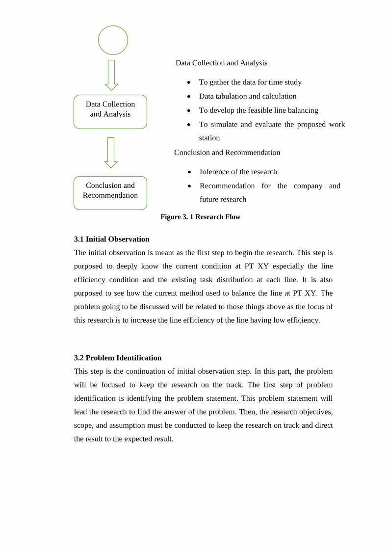
Data Collection
and Analysis
Conclusion and
Recommendation
Data Collection and Analysis
To gather the data for time study
Data tabulation and calculation
To develop the feasible line balancing
To simulate and evaluate the proposed work
station
Conclusion and Recommendation
Inference of the research
Recommendation for the company and
future research
Figure 3. 1 Research Flow

3.3 Literature Study
The literature study is conducted as the learning material in developing the
research. This step will be very important as the way method works and how is it
done are stated in this phase. This will also help to determine what kind of data
should be gathered. It is difficult to develop something without any knowledge as
the basis of research development. Literature study can also be the direction of the
research development.
There are some concern will be discussed through the literature study in this
research. The major concern will be about time study, line balancing, and its
simulation. The time study will include the normal time, allowance, together with
normality test, sufficiency test, and uniformity test. The line balancing will
include the line balancing method together with the measurement of line
balancing.
3.4 Data Collection and Analysis
This step can be divided into two phases. The first the collection of data and then
followed by the analysis of the data collected.
3.4.1 Data Collection
Data of existing method of line balancing problem solving related to Line
M123 Operation Process Chart of Toy DJ123 as the chart will inform how
the assembly process works
The operation method used by the operator at line M123 and it is detailed
with the standard time and the motion for each operation.
Work allowance based on establishment by PT XY
The efficiency target established by PT XY
There are some of collections of data that will be counted by again to support
the analysis of the research:
Time study for each operation using stop watch for some items.
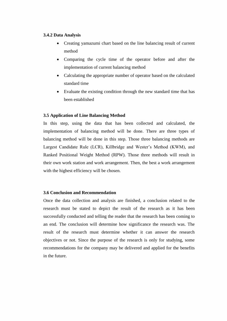
3.4.2 Data Analysis
Creating yamazumi chart based on the line balancing result of current
method
Comparing the cycle time of the operator before and after the
implementation of current balancing method
Calculating the appropriate number of operator based on the calculated
standard time
Evaluate the existing condition through the new standard time that has
been established
3.5 Application of Line Balancing Method
In this step, using the data that has been collected and calculated, the
implementation of balancing method will be done. There are three types of
balancing method will be done in this step. Those three balancing methods are
Largest Candidate Rule (LCR), Killbridge and Wester’s Method (KWM), and
Ranked Positional Weight Method (RPW). Those three methods will result in
their own work station and work arrangement. Then, the best a work arrangement
with the highest efficiency will be chosen.
3.6 Conclusion and Recommendation
Once the data collection and analysis are finished, a conclusion related to the
research must be stated to depict the result of the research as it has been
successfully conducted and telling the reader that the research has been coming to
an end. The conclusion will determine how significance the research was. The
result of the research must determine whether it can answer the research
objectives or not. Since the purpose of the research is only for studying, some
recommendations for the company may be delivered and applied for the benefits
in the future.

Start
Observation
Found a line with
low efficiency?
Literature Study
Root cause
analysis using fish
bone
Record cycle time
Normality Test
Normal Data ?
Uniformity Test
Uniform Data?
Sufficiency Test
Sufficient
Data?
Calculate Normal
Time and Std Time
Apply LCR, KWM,
and RPW method
Compare the
efficiency of those
LB methods
Choose the best
method
Additional action to
make the CT more
balance
Achieve 90%
efficiency?
Compare current
vs proposed work
arrangement
Conclusion and
Recommendation
End
3.7Research Framework
Figure 3. 2 Research Framework
CHAPTER IV
DATA COLLECTION AND ANALYSIS
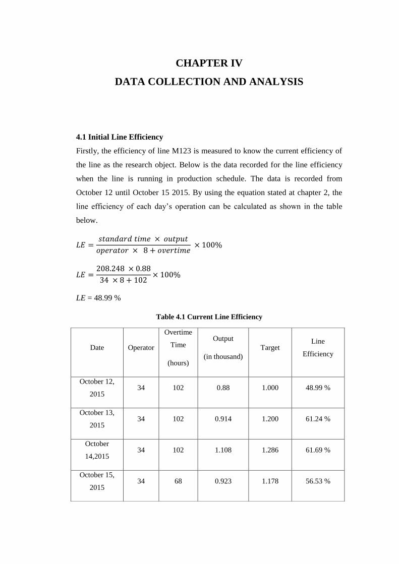
4.1 Initial Line Efficiency
Firstly, the efficiency of line M123 is measured to know the current efficiency of
the line as the research object. Below is the data recorded for the line efficiency
when the line is running in production schedule. The data is recorded from
October 12 until October 15 2015. By using the equation stated at chapter 2, the
line efficiency of each day’s operation can be calculated as shown in the table
below.
LE = 48.99 %
Table 4.1 Current Line Efficiency
Date Operator
Overtime
Time
(hours)
Output
(in thousand)
Target Line
Efficiency
October 12,
2015 34 102 0.88 1.000 48.99 %
October 13,
2015 34 102 0.914 1.200 61.24 %
October
14,2015 34 102 1.108 1.286 61.69 %
October 15,
2015 34 68 0.923 1.178 56.53 %

Looking at the data above, the average of line efficiency can be calculated.
The line efficiency above is still considered low. It can be seen that it is far from
the company’s target. Logically, using the standard time determined by the
company, to achieve 100% efficiency in producing 1000 units of product per
shift, using the same efficiency calculation, it is supposed to be:
The calculation above shows that it will only need 27 operators to produce 1000
units of product to do it smoothly. In fact, the actual condition shows that it
utilizes up to 34 operators with overtime up to 3 hours for each operator.
4.2 Analyzing Root Cause of Low Efficiency
Low Line
Effieciency
Man
Operator’s time
In each work station
Is not balance
Material
Head is not available
When operator is
About to assembly
MachineMethod
Production output
Is not achieved
Operator can’t
Follow the sequence of
Working like stated
In the guidance
Late head supply
Poor work
arrangement
Different condition
Between guidance
And actual
Inappropriate
Number of operatorHigh cycle time on
Some operators
Std time
Determined is
Not suitable
Figure 4. 1 Fishbone Diagram of Root Cause Analysis
Average 57.11%

1. Man
In terms of man, actually, the number of man assigned to do the final
assembly process of toy DJ123 is already high. But, the target of
production output cannot still be fulfilled. There must be something wrong
with the man assigned to do the final assembly process.
After doing the observation, the skill of people who work for this process
is not equally-likely between one operator and the other operators. Thus,
the standard time in finishing the product between one operator to another
operator may vary. Thus, to overcome this problem, the standard time
determined later should consider the performance rating of each operator
working on each element which is expected to find the most appropriate
number of operator. Finding the most appropriate number is one of the
focus of this research.
2. Machine
In terms of machine, there seems to be no problem since not all operators
utilize machine during the final assembly process. During the observation
time, there is no problem found related to machine operation. So, it can be
concluded that the machine has no problem for this case.
3. Material
In terms of material, some problem is found related to this point. At the
first day of observation, the head part is lately distributed to the production
line. The roto (head) supply from rotocast area is lately distributed to
production line. There was some problem related to supply material to
rotocast area.
4. Method
There are some problems can be described related to method. In doing the
final assembly process of toy DJ123, of course there are some methods
implemented for the process. This method has actually been established by
Industrial Engineering Department. In fact, what actually happen in the
Production line is different with what has been established. This happen

because the target output is different with what has been set. The labor
data sheet appears to show 750 per shift. But, the actual production
process appears to be 1000 units per shift. So, the operators applied some
unstandardized method improvement which is different with what has
been determined by the IE department. The method is also related to the
layout. In this case, the layout is not well arranged. Moreover, some of the
position of operators doing the process is separated. The layout
arrangement is not really good. There is also variance between the actual
time needed in each process and the time stated in the standard. Thus, the
focus will be on finding the most accurate standard time for the work
element.
4.2.1 Observing the Standard Determined by Company
As have been stated before, the real condition of what the production line has been
doing is not the same anymore with what has been plant for the toy DJ123.
Table 4.2 Labor Data Sheet
Code Operator Operations
O-1 1 Date code torso
O-2 Dressing
O-3 Attaching torso to belt
O-4 Assy cape
O-5 2 Cutting polybag
O-6 Grooming hair
O-7 Release rubberband
O-8 3 Hair arrangement
O-9 Hair cutting
O-10 4 Hair setting
O-11 Pegboard extension
O-12 5 Releasing tule
O-13 Trimming
O-14 6 Attach shoes to torso

O-15 Attach to hand
O-16 Tack head to support
Table 4.2 Labor Data Sheet
Code Operator Operations
O-17 7 Fold insert
O-18 Attach to Insert
O-19 8 Lock tab
O-20 Tie down hair
O-21 Lock separator
O-22 9 Dressing torso
O-23 Attach arm
O-24 10 Assembly torso belt
O-25 Attaching to hand
O-26 Join head
O-27 11 Lock toralei support
O-28 Elastic staples
O-29 12 Assembly C
O-30 Elastic staples
O-31 13 Spotweld tab
O-32 Attach to Insert
O-33 14 Touch up
O-34 Put Blister
O-35 15 Locking blister
O-36 Pack to MC
R factor = 34.5 (Takt time based on LDS)
Standard Demand at LDS = 750 units
Hours / shift = 8
Quantity per shift = 750

The table above shows the code name operation of each work element in toy
DJ123. The coding system using O-1, O-2, O-3, and etc is purposed to simplify
the name of each work element in the process of final assembling toy DJ123.
After the breakdown, in total there are 36 operations to complete toy DJ123
assembly process. The actual work arrangement is actually shown at the Labor
Data Sheet. Below is the work arrangement.
Table 4.3 Work Arrangement Based on Labor Data Sheet
Work
Station Operation
Cycle
Time
(s)
Number
of
Operator
CT per
Work
Station
1 O-1 + O-2 + O3 +O4 41.04 1 41.04
2 O-5 + O-6 + O-7 63.18 2 31.59
3 O-8 + O-9 77.94 2 38.97
4 O-10 + O-11 41.4 1 41.4
5 O-12 + O-13 30.84 1 30.84
6 O-14 + O-15 + O-16 40.32 1 40.32
7 O-17 + O-18 31.92 1 31.92
8 O-19 + O-20 + O-21 34.56 1 34.56
9 O-22 + O-23 40.5 1 40.5
10 O-24 + O-25 + O-26 39.36 1 39.36
11 O-27 + 28 37.98 1 37.98
12 O-29 + O-30 39.18 1 39.18
13 O-31 + O-32 38.52 1 38.52
14 O-33 + O-34 34.38 1 34.38
15 O-35 + O-36 39.84 1 39.84
Total Operator 17
Above is the work arrangement proposed by Labor Data Sheet. Based on the
Labor Data Sheet, the total operator needed is only 17. As have been stated
before, Labor Data Sheet is only designed for the 750 demand with 8 working
hours. It means that it can’t cover the actual operation which needs 1000 units to
be produced and in fact, the 8 working hours is not enough.

In any kind of operation, the standard must have been built to accomplish the
target. In running this toy, there is also a standard as the guidance for operator in
producing this toy, the standard itself is Labor Data Sheet (LDS).
The operators usually work based on Labor Data Sheet as it is a document
developed as the guidance of running the toy in Production Schedule. Below is the
data Labor Data Sheet of toy DJ123
Figure 4. 2 Yamazumi of Labor Data Sheet
Looking at the Labor Data Sheet developed for the guidance of operator, it can
clearly be seen that the work is not appropriately distributed. The R-Factor which
is also known as determined takt time is 34.5 s and the other data represent the
time that must be accomplished for each operation.
Looking at the data distribution, it turns out that there are many cycle times below
the determined takt time and there are also many cycle times above the takt time.
It is impossible for example in operation 1, 2,3,4,5 to do the task much longer
than required one. That is why the yamazumi chart itself for the Labor Data Sheet
is not yet balance.
Looking at the Labor Data Sheet again, the quantity per shift set for this toy is 750
toys and is not suitable with the reality when the production line running. This is
why the line leader does not have any guidance when the production running with
the bigger quantity of toy produced. That is why the line leader seems like lost
guidance during the production process.
0
10
20
30
40
50
1 2 3 4 5 6 7 8 9 10 11 12 13 14 15
Cyc
le T
ime
(S)
Work Station
CT per WorkStation
TT
The reason why work distribution is not balance because this Labor Data Sheet is
designed before the toy is mass produced and it is not repaired when the toy is
mass produced. It is why the further time study is needed to make the appropriate
Labor Data Sheet (LDS).
4.2.3 Number of Operator
Evaluation of the number of operator must also be evaluated to determine the
appropriate number of doing overall operation. The number of operator cannot be
over and cannot be less otherwise it can affect the efficiency of the operation. The
formula of determining number of operator has been explained in chapter 2.
N = 21.419 = 22
Based on the Labor Data Sheet, the appropriate number of operator must be 22
operators. It is impossible to have 21.419 operators so it has to be rounded up to
22 operators. 738.98 is the total cycle time needed to run the full operation of toy
DJ123 and 34.5 is the takt time determined by Labor Data Sheet. So, the number
of operator must have been a problem for this toy.
In fact, the LDS only provide 17 operators which are totally insufficient to have
such a standard determined. To gain a good efficiency, the number of operators
must be added 5 people.
4.3 Standard Time at M123
The standard time used must also be analyzed to find the correlation with the low
efficiency that happens at this line. The data designed at the Labor Data Sheet
must be analyzed whether it is math with the actual condition in the production
line. The data from the Labor Data Sheet itself is usually from the pre-determined
time for each operation. In this part, the comparison between the time from Labor
Data Sheet and actual at 555 kaizen will be tried to be analyzed.
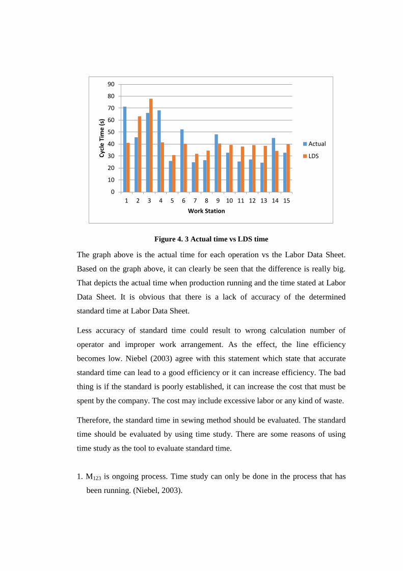
Figure 4. 3 Actual time vs LDS time
The graph above is the actual time for each operation vs the Labor Data Sheet.
Based on the graph above, it can clearly be seen that the difference is really big.
That depicts the actual time when production running and the time stated at Labor
Data Sheet. It is obvious that there is a lack of accuracy of the determined
standard time at Labor Data Sheet.
Less accuracy of standard time could result to wrong calculation number of
operator and improper work arrangement. As the effect, the line efficiency
becomes low. Niebel (2003) agree with this statement which state that accurate
standard time can lead to a good efficiency or it can increase efficiency. The bad
thing is if the standard is poorly established, it can increase the cost that must be
spent by the company. The cost may include excessive labor or any kind of waste.
Therefore, the standard time in sewing method should be evaluated. The standard
time should be evaluated by using time study. There are some reasons of using
time study as the tool to evaluate standard time.
1. M123 is ongoing process. Time study can only be done in the process that has
been running. (Niebel, 2003).
0
10
20
30
40
50
60
70
80
90
1 2 3 4 5 6 7 8 9 10 11 12 13 14 15
Cyc
le T
ime
(s)
Work Station
Actual
LDS
2. Time study is simpler to be done and accurate (Niebel, 2003).
From this analysis, it is found that the poor work arrangement and less accuracy of
standard time have become the root cause of having low line efficiency. Since the
work arrangement is depend on the standard time, increasing the accuracy of
standard time has to be done prior to redesigning the work arrangement. By
having more accurate standard time, it is expected to have adequate number of
operators and proper work arrangement. Thus, time study is discussed first.
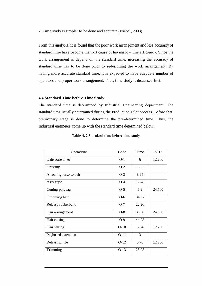
4.4 Standard Time before Time Study
The standard time is determined by Industrial Engineering department. The
standard time usually determined during the Production Pilot process. Before that,
preliminary stage is done to determine the pre-determined time. Thus, the
Industrial engineers come up with the standard time determined below.
Table 4. 2 Standard time before time study
Operations Code Time STD
Date code torso O-1 6 12.250
Dressing O-2 13.62
Attaching torso to belt O-3 8.94
Assy cape O-4 12.48
Cutting polybag O-5 6.9 24.500
Grooming hair O-6 34.02
Release rubberband O-7 22.26
Hair arrangement O-8 33.66 24.500
Hair cutting O-9 44.28
Hair setting O-10 38.4 12.250
Pegboard extension O-11 3
Releasing tule O-12 5.76 12.250
Trimming O-13 25.08

The table above is the standard time obtained from the Operation Process Chart
(OPC). By having Operation Process Chart, the process is expected to be seen
clearly. The Operation Process Chart (OPC) is shown at appendix 1.
Attach shoes to torso O-14 8.16 12.250
Attach to hand O-15 24.78
Tack head to support O-16 7.38
Fold insert O-17 15.12 12.250
Attach to Insert O-18 16.8
Lock tab O-19 5.28
12.250 Tie down hair O-20 24
Lock separator O-21 5.28
Table 4.2 Standard time before time study (continued)
Dressing torso O-22 20.88 12.250
Attach arm O-23 19.62
Assembly torso belt O-24 15.24
12.250 Attaching to hand O-25 18.42
Join head O-26 5.7
Lock toralei support O-27 10.86 12.250
Elastic staples O-28 27.12
Assembly C O-29 10.68 12.250
Elastic staples O-30 28.5
Spotweld tab O-31 12.06 12.250
Attach to Insert O-32 26.46
Touch up O-33 23.88 12.250
Put Blister O-34 10.5
Locking blister O-35 29.04 12.250
Pack to MC O-36 10.8
Total Standard Hours 630.9 208.248

4.5 Actual Standard Time
4.5.1 Normality Test
The normality test is done using minitab 17. In normality time, the thing that is
concerned most is the P-Value. The time study result is inputted to the minitab
application and the minitab 17 will automatically do the analysis. The result will
directly be shown. For this final project, the level of significance for the data is
0.05. So, if it is found that the P-Value of time study for each work element bigger
than 0.05, “fail to reject H0” is the conclusion. However, if the P-Value is lower
than 0.05, the conclusion must be “reject H0 or “accept HA”.
For example looking at the operation 1 (O-1), the P-Value is shown to be 0.836. It
means the P-Value is greater than 0.05, then the conclusion is “fail to reject H0”.
So the data can said normally distributed. Some of the data may not pass the
normal distribution test at the beginning, so the data must be collected again until
the P-Value result shown by minitab 17 becomes greater than 0.05. For example,
the data at Operation 3 (O-3) firstly showed 0.013 as the P-Value. Thus, the
conclusion must be “reject H0” which mean the data collected for O-3 is not
normally distributed. So, stop watch time study must be conducted again for O-3
until the P-Value become greater than 0.05. The attached Normality data test is
already been completed and all the data shown in the appendix is already normally
distributed for all operation.
4.5.2 Uniformity Test
A set of data may be considered normally distributed, but it is not going to be
good with wide variance. Thus, after dealing with normality test, the next step
should be uniformity test. In uniformity test, upper and lower limit must be
determined to figure out whether the data uniform or not. The formula has been
stated at chapter 2. To determine the upper and lower limit, the standard deviation
must firstly be found. Then, to achieve 99% area normal distribution, six sigma
theorems is used by using three times of standard deviation for upper and lower
limit from the mean of the data. That is the way to determine the upper and lower
limit of the data.
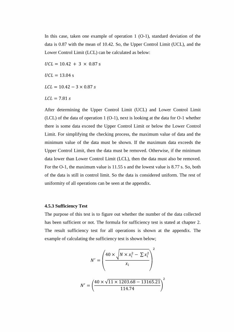
In this case, taken one example of operation 1 (O-1), standard deviation of the
data is 0.87 with the mean of 10.42. So, the Upper Control Limit (UCL), and the
Lower Control Limit (LCL) can be calculated as below:
s
After determining the Upper Control Limit (UCL) and Lower Control Limit
(LCL) of the data of operation 1 (O-1), next is looking at the data for O-1 whether
there is some data exceed the Upper Control Limit or below the Lower Control
Limit. For simplifying the checking process, the maximum value of data and the
minimum value of the data must be shown. If the maximum data exceeds the
Upper Control Limit, then the data must be removed. Otherwise, if the minimum
data lower than Lower Control Limit (LCL), then the data must also be removed.
For the O-1, the maximum value is 11.55 s and the lowest value is 8.77 s. So, both
of the data is still in control limit. So the data is considered uniform. The rest of
uniformity of all operations can be seen at the appendix.
4.5.3 Sufficiency Test
The purpose of this test is to figure out whether the number of the data collected
has been sufficient or not. The formula for sufficiency test is stated at chapter 2.
The result sufficiency test for all operations is shown at the appendix. The
example of calculating the sufficiency test is shown below;
(
√
∑
)
( √
)

Based on the result of sufficiency test, the number of observation that must be
done for operation 1 (O-1) is 10. In fact, the data taken for operation 1 (O-1) is 11.
So, it is considered that the data is enough and pass the sufficiency test.
4.5.4 Performance Rating
It is known that the performance rating is one of the factors to get the normal time.
Performance rating can vary from one operator to other operators. The evaluation
of performance rating can be very useful to determine normal time. Niebel (2003)
mentioned four factors in evaluating the performance of the operator; skill, effort,
condition, and consistency. It assumed that all the operators who become the
object of time study are considered to have the same average condition and valued
as D with 0.00 point. So, only skills, effort, and consistency are evaluated. Those
are evaluated the line leader. The table below is the example of performance
rating calculation for the operator who is responsible for O-1
Table 4. 3 Performance of Operator 1
Skill C2 0.03
Effort C2 0.02
Condition D 0
Consistency C 0.01
Algebraic Sum 0.06
Performance Factor
1.06
Toy DJ123 is one of the toys with the most complicated process. It is found that
no operator has the performance rating below 1 which mean the operator observed
for time study do the process within or below the normal time. For more detail, it
can be seen at the appendix 4.

4.5.5 Normal Time
After dealing with all the evaluations above starting from normality test,
uniformity test, sufficiency test, until the performance rating, the next step is
determining the normal time for each operations. All the evaluations above will be
used to determine the normal time. Normal time itself is obtained by multiplying
mean time with performance rating of the operators as defined in equation. The
data shows that more skillful and consistent the operator, the bigger the effort, the
bigger the normal time will be. Calculation of normal time is done like below;
Above is the example of calculating standard time. The average of operation 1 (O-
1) is 10.43 and the performance rating of operator observed assessed by the line
leader is 1.06. Thus, the normal time is the multiplication of average and
performance rating with the result of 11.06 s.
4.5.6 PFD (Personal, Fatigue, and Delay)
For the personal matter, fatigue and delay, PT XY has already had its own study
to determine this allowance. The allowance is determined for each area including
the final assembly area. The allowance is 11.2 %. This allowance covers personal,
fatigue, and delay allowance.
4.5.7 Standard Time
Standard time is obtained after finding the allowance because in the real life, no
operators can do the task 8 hours full without any delay or getting distracted. The
way to calculate the standard time has been stated on chapter 2. Using the
equation, the standard time can be calculated as below;

Table 4. 4 Actual Standard Time
Code Process Second per
unit
O-1 Date code torso 12.30
O-2 Dressing 29.04
O-3 Attaching torso to belt 17.99
O-4 Assy cape 25.39
O-5 Cutting polybag 5.41
O-6 Grooming hair 29.28
O-7 Release rubberband 18.81
O-8 Hair arrangement 33.80
O-9 Hair cutting 44.46
O-10 Hair setting 76.56
O-11 Pegboard extension 6.00
O-12 Releasing tule 5.73
O-13 Trimming 25.28
O-14 Attach shoes to torso 12.48
O-15 Attach to hand 37.45
O-16 Tack head to support 11.51
O-17 Fold insert 13.89
O-18 Attach to Insert 16.04
O-19 Lock tab 5.00
O-20 Tie down hair 21.42
Table 4.4 Actual Standard Time (continued)
Code Process Second per
unit
O-21 Lock separator 4.88
O-22 Dressing torso 29.78
O-23 Attach arm 27.24
O-24 Assembly torso belt 15.25
O-25 Attaching to hand 18.41
O-26 Join head 5.56
O-27 Lock toralei support 8.45
O-28 Elastic staples 21.08
O-29 Assembly C 8.61
O-30 Elastic staples 23.44
O-31 Spotweld tab 9.04
O-32 Attach to Insert 20.19
O-33 Touch up 36.35
O-34 Put Blister 15.25
O-35 Locking blister 28.71
O-36 Pack to MC 10.44
Total time 730.50

Based on the table above, the new standard time has been obtained for every work
element. It can be seen that the standard time per unit has been increased from
630.9 s to 730.50 s. It means that the difference between the actual time and
standard time obtained by time study is different.
4.6 Line Balancing
The next step must be one of the most important parts of this research. The next
step is about line balancing method application. To ensure the result and
providing several solutions, the line balancing analysis will be done through 3
different method application; they are Largest Candidate Rule (LCR), Killbridge
and Wester Method (KWM), and Ranked Positional Weigh (RPW).
Since there is no certain standard for how many available times allowed in a day,
thus the takt time for the line balancing process is considered as below:
It is considered the assumed that the allowed over time is 2 hours because among
the 4 days operation, the lowest overtime is 2 hours. The toy is designed to run for
750 toys per shift but in fact, the number of toy that must be produced is 1000
units. Looking at that fact, the takt time used is considered to be the same as the
actual operation.
4.6.1 Largest Candidate Rule
Largest candidate rule is started by using the precedence table consists of
predecessor and successor. The precedence diagram contains information about
the sequence of process in final assembly process of toy DJ1123. The precedence
diagram will also be used in the other method as the basic information of the final

assembly process. For more detail, the information of precedence diagram is
shown below

5
6
22
1
8
9
31
7 17 18 19 20 21
23 24 25 26
2 3 4 14 15 16 27
10 11 12 13 28 29 30 33 34 35
32
36
Figure 4. 4 Precedence Diagram
46

Table 4. 5 Precedence Table
No Operation Te Immediate Predecessor
1 O-5 5.41 -
2 O-6 29.28 -
3 O-22 29.78 -
4 O-1 12.30 -
5 O-8 33.80 -
6 O-9 44.46 -
7 O-31 9.04 -
8 O-7 18.81 O-5 O-,6
9 O-23 27.24 O-22
10 O-2 29.04 O-1
11 O-10 76.56 O-8, O-9
12 O-32 20.19 O-31
13 O-17 13.89 O-5, O-6, O-7
14 O-3 17.99 O-1, O-2
15 O-11 6.00 O-8, O-9, O-10
16 O-18 16.04 O-5, O-6, O-7, O-17
17 O-4 25.39 O-1, O-2, O-3
18 O-12 5.73 O-8, O-9, O-10, O-11
19 O-19 5.00 O-5, O-6, O-7, O-17, O-18
20 O- 13 25.28 O-8, O-9, O-10, O-11, O-12
21 O-20 21.42 O-5, O-6, O-7, O-17, O-18, O-19
22 O-14 12.48 O-1, O-2, O-3, O-4, O-8, O-9, O-10, O-11, O-12, O-13
23 O-21 4.88 O-5, O-6, O-7, O-17, O-18, O-19, O-20
24 O-15 37.45 O-1, O-2, O-3, O-4, O- 8, O-9, O-10, O-11, O-12, O-13, O-14
25 O-24 15.25 O-5, O-6, O-7, O-17, O-18, O-19, O-20, O-21, O-22, O-23
26 O-16 11.51 O-1, O-2, O-3, O-4, O-8, O-9, O-10, O-11, O-12, O-13, O-14,
O-15
27 O-25 18.41 O-5, O-6, O-7, O-17, O-18, O-19, O-20, O-21, O-22, O-23,
O-24
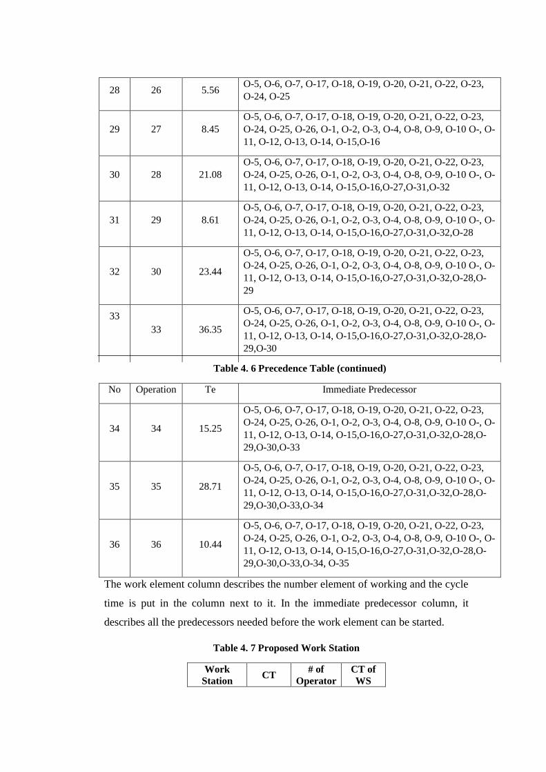
28 26 5.56 O-5, O-6, O-7, O-17, O-18, O-19, O-20, O-21, O-22, O-23,
O-24, O-25
29 27 8.45
O-5, O-6, O-7, O-17, O-18, O-19, O-20, O-21, O-22, O-23,
O-24, O-25, O-26, O-1, O-2, O-3, O-4, O-8, O-9, O-10 O-, O-
11, O-12, O-13, O-14, O-15,O-16
30 28 21.08
O-5, O-6, O-7, O-17, O-18, O-19, O-20, O-21, O-22, O-23,
O-24, O-25, O-26, O-1, O-2, O-3, O-4, O-8, O-9, O-10 O-, O-
11, O-12, O-13, O-14, O-15,O-16,O-27,O-31,O-32
31 29 8.61
O-5, O-6, O-7, O-17, O-18, O-19, O-20, O-21, O-22, O-23,
O-24, O-25, O-26, O-1, O-2, O-3, O-4, O-8, O-9, O-10 O-, O-
11, O-12, O-13, O-14, O-15,O-16,O-27,O-31,O-32,O-28
32 30 23.44
O-5, O-6, O-7, O-17, O-18, O-19, O-20, O-21, O-22, O-23,
O-24, O-25, O-26, O-1, O-2, O-3, O-4, O-8, O-9, O-10 O-, O-
11, O-12, O-13, O-14, O-15,O-16,O-27,O-31,O-32,O-28,O-
29
33
33 36.35
O-5, O-6, O-7, O-17, O-18, O-19, O-20, O-21, O-22, O-23,
O-24, O-25, O-26, O-1, O-2, O-3, O-4, O-8, O-9, O-10 O-, O-
11, O-12, O-13, O-14, O-15,O-16,O-27,O-31,O-32,O-28,O-
29,O-30
Table 4. 6 Precedence Table (continued)
No Operation Te Immediate Predecessor
34 34 15.25
O-5, O-6, O-7, O-17, O-18, O-19, O-20, O-21, O-22, O-23,
O-24, O-25, O-26, O-1, O-2, O-3, O-4, O-8, O-9, O-10 O-, O-
11, O-12, O-13, O-14, O-15,O-16,O-27,O-31,O-32,O-28,O-
29,O-30,O-33
35 35 28.71
O-5, O-6, O-7, O-17, O-18, O-19, O-20, O-21, O-22, O-23,
O-24, O-25, O-26, O-1, O-2, O-3, O-4, O-8, O-9, O-10 O-, O-
11, O-12, O-13, O-14, O-15,O-16,O-27,O-31,O-32,O-28,O-
29,O-30,O-33,O-34
36 36 10.44
O-5, O-6, O-7, O-17, O-18, O-19, O-20, O-21, O-22, O-23,
O-24, O-25, O-26, O-1, O-2, O-3, O-4, O-8, O-9, O-10 O-, O-
11, O-12, O-13, O-14, O-15,O-16,O-27,O-31,O-32,O-28,O-
29,O-30,O-33,O-34, O-35
The work element column describes the number element of working and the cycle
time is put in the column next to it. In the immediate predecessor column, it
describes all the predecessors needed before the work element can be started.
Table 4. 7 Proposed Work Station
Work
Station CT
# of
Operator
CT of
WS
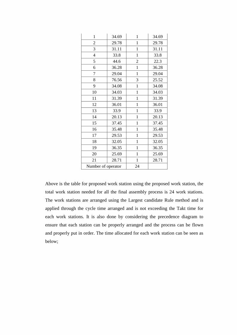
1 34.69 1 34.69
2 29.78 1 29.78
3 31.11 1 31.11
4 33.8 1 33.8
5 44.6 2 22.3
6 36.28 1 36.28
7 29.04 1 29.04
8 76.56 3 25.52
9 34.08 1 34.08
10 34.03 1 34.03
11 31.39 1 31.39
12 36.01 1 36.01
13 33.9 1 33.9
14 20.13 1 20.13
15 37.45 1 37.45
16 35.48 1 35.48
17 29.53 1 29.53
18 32.05 1 32.05
19 36.35 1 36.35
20 25.69 1 25.69
21 28.71 1 28.71
Number of operator 24
Above is the table for proposed work station using the proposed work station, the
total work station needed for all the final assembly process is 24 work stations.
The work stations are arranged using the Largest candidate Rule method and is
applied through the cycle time arranged and is not exceeding the Takt time for
each work stations. It is also done by considering the precedence diagram to
ensure that each station can be properly arranged and the process can be flown
and properly put in order. The time allocated for each work station can be seen as
below;

Figure 4. 5 Yamazumi Chart of LCR Method Application
It can be seen from the chart that the cycle time of each operation has almost all
lay down below the takt time. But there is one problem when two of the operation
still exceeds the takt time as the process is known to have a long cycle time. The
other solution to balance the and reduce the cycle time is by separating the process
or moving some process with high cycle time to the work station with the lowest
cycle time. It is actually kind of practical since the theory only by using
precedence diagram will not be enough to determine which process can be moved
or reduced. The more consultation and trial with the field executor must be done.
But, before doing so, let’s first compare the line balancing result between three
methods.
0
5
10
15
20
25
30
35
40
1 2 3 4 5 6 7 8 9 101112131415161718192021
Cyc
le T
ime
(s)
Work Station
CT of WS
TT
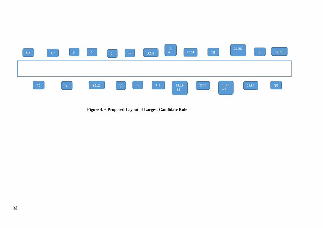
5,6
22
1,7
8
9
31,23
2 9
10
32,17
3,18
11,4 10
10 12,19,13
20,14
21,24
15
16,25,26
27,28
29,30
33 34,36
35
Figure 4. 6 Proposed Layout of Largest Candidate Rule
50

4.6.1.1 Evaluation of Largest Candidate Rule
To ensure the performance of the line arrangement proposed, the result of
arrangement must also be evaluated by calculating the smoothness index and the
balance delay of the line arrangement proposed.
Table 4. 8 Evaluation of LCR
Operator CT (CTi-CT max)2
1 34.69 7.6176
2 29.78 58.8289
3 31.11 40.1956
4 33.8 13.3225
5 22.3 229.5225
6 22.3 229.5225
7 36.28 1.3689
8 29.04 70.7281
9 25.52 142.3249
10 25.52 142.3249
11 25.52 142.3249
12 34.08 11.3569
13 34.03 11.6964
14 31.39 36.7236
15 36.01 2.0736
16 33.9 12.6025
17 20.13 299.9824
18 37.45 0
19 35.48 3.8809
20 29.53 62.7264
21 32.05 29.16
22 36.35 1.21
23 25.69 138.2976
24 28.71 76.3876
Total 730.66 1764.18
√
Based on the smoothness calculation, it is obtained that the result of smoothness
index is 42.002. Theoretically, the lower the smoothness index the better it is. To

obtain the smoothness index, each cycle time in each work station must be
subtracted by the highest cycle time in all operations then square the result.
Station 1
Balance Delay
After dealing with the smoothness index, the next is calculating the balance delay.
Using the Largest Candidate Rule method, the balance delay found is to be
18.71% which result only 81.29% of line efficiency. The balance delay is
calculated using the formula above.

4.6.2 Killbridge and Wester Method
Figure 4. 7 Killbridge and Wester Method
53

Table 4. 9 Killbridge and Wester Method
Work
Station Operation CT
CT per work
station
Number of
Operator
1 O-5 5.41
34.70 1 O-6 29.28
2 O-7 18.81
32.70 1 O-17 13.89
3 O-22 29.78 29.78 1
4 O-23 27.24 27.24 1
5 O-1 12.30 12.30 1
6 O-2 29.04
35.03 1 O-11 6.00
7 O-8 33.80 33.80 1
8 O-9 44.46 22.23 2
9 O-10 76.56 25.5 3
10 O-31 9.04
29.24 1 O-32 20.19
11 O-3 17.99
34.03 1 O-18 16.04
12 O-4 25.39
31.12 1 O-12 5.73
13 O-13 25.28
30.27 1 O-19 5.00
14 O-14 12.48
33.90 1 O-20 21.42
15 O-21 4.88
20.13 1 O-24 15.25
16 O-15 37.45 37.45 1
17
O-16 11.51
35.48 1 O-25 18.41
O-26 5.56
18 O-27 8.45
29.53 1 O-28 21.08
19 O-29 8.61
32.05 1 O-30 23.44
20 O-33 36.35 36.35 1
21 O-34 15.25 15.25 1
22 O-35 28.71 28.71 1
23 O-36 10.44 10.44 1
Total Operators needed 26
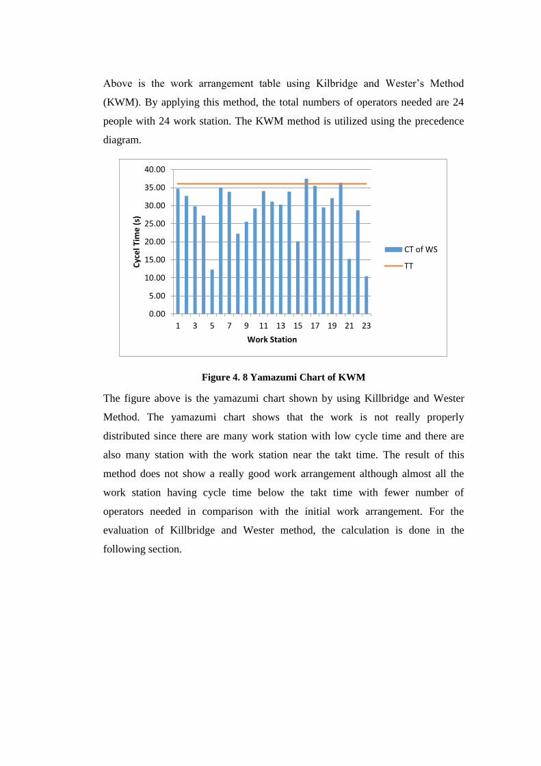
Above is the work arrangement table using Kilbridge and Wester’s Method
(KWM). By applying this method, the total numbers of operators needed are 24
people with 24 work station. The KWM method is utilized using the precedence
diagram.
Figure 4. 8 Yamazumi Chart of KWM
The figure above is the yamazumi chart shown by using Killbridge and Wester
Method. The yamazumi chart shows that the work is not really properly
distributed since there are many work station with low cycle time and there are
also many station with the work station near the takt time. The result of this
method does not show a really good work arrangement although almost all the
work station having cycle time below the takt time with fewer number of
operators needed in comparison with the initial work arrangement. For the
evaluation of Killbridge and Wester method, the calculation is done in the
following section.
0.00
5.00
10.00
15.00
20.00
25.00
30.00
35.00
40.00
1 3 5 7 9 11 13 15 17 19 21 23
Cyc
el T
ime
(s)
Work Station
CT of WS
TT
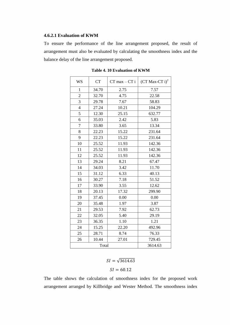
4.6.2.1 Evaluation of KWM
To ensure the performance of the line arrangement proposed, the result of
arrangement must also be evaluated by calculating the smoothness index and the
balance delay of the line arrangement proposed.
Table 4. 10 Evaluation of KWM
WS CT CT max – CT i (CT Max-CT i)2
1 34.70 2.75 7.57
2 32.70 4.75 22.58
3 29.78 7.67 58.83
4 27.24 10.21 104.29
5 12.30 25.15 632.77
6 35.03 2.42 5.83
7 33.80 3.65 13.34
8 22.23 15.22 231.64
9 22.23 15.22 231.64
10 25.52 11.93 142.36
11 25.52 11.93 142.36
12 25.52 11.93 142.36
13 29.24 8.21 67.47
14 34.03 3.42 11.70
15 31.12 6.33 40.13
16 30.27 7.18 51.52
17 33.90 3.55 12.62
18 20.13 17.32 299.90
19 37.45 0.00 0.00
20 35.48 1.97 3.87
21 29.53 7.92 62.73
22 32.05 5.40 29.19
23 36.35 1.10 1.21
24 15.25 22.20 492.96
25 28.71 8.74 76.33
26 10.44 27.01 729.45
Total 3614.63
√
The table shows the calculation of smoothness index for the proposed work
arrangement arranged by Killbridge and Wester Method. The smoothness index

obtained is not significantly good since the number obtained is 60.12. For the
smoothness index calculation, the lower the smoothness index, the better it will
be.
Balance Delay
The calculation of balance delay is done to get the clear picture of the delay of the
process can be. Through the application of Killbridge and Wester Method, the
balance delay is obtained to be 25% which is not very good and cannot fulfill the
efficiency target determined by the company. The balance delay calculation can
be obtained through the application of formula stated on chapter 2.
By obtaining the balance delay, the efficiency of the line can roughly be obtained
by looking of the percentage remaining. Looking at the calculation above, the line
efficiency can be said to be 75% since the balance delay obtained through
Killbridge and Westers Method is 25%.
4.6.3 Rank Positional Weight
To calculate the Rank Position weight, calculating the weight is a must to be done.
Below is the example of how to calculate the positional weight:
O-1 + O-2 + O-3 + O-4 + O-14 + O-15 + O-16 + O-27 + O-28 + O-29 + O-30
+ O-33 + O-34 + O-35 + O-36
12.30 + 29.04 + 17.99 + 25.39 + 12.48 + 37.45 + 11.51 + 8.45 + 21.08 + 8.61 +
23.44 + 36.35 + 15.25 + 28.71 + 10.44 = 298.74
Based on the calculation, it can be seen that the weight for operation 1 (O-1) is
298.74. The detail RPW matrix is given on appendix 9.

Table 4. 11 Work Station of RPW Application
No Operation Cycle Time Number of
Operator
Cycle time per
workstation
1 O-9 44.46 2 22.23
2 O-8 33.8 1 33.8
3 O-10 76.56 3 25.52
4 O-6 29.28 1 29.28
5 O-1 12.3
1
31.11 O-7 18.81
6 O-2 29.04
1
34.45 O-5 5.41
7 O-3 17.99
1
31.888 O-17 13.898
8 O-11 6
1
35.78 O-22 29.78
9 O-12 5.73
1
31.12 O-4 25.39
10 O-13 25.28
1
30.28 O-19 5
11 O-18 16.04
1
28.52 O-14 12.48
12 O-23 27.24
1
32.12 O-21 4.88
13 O-20 21.42
1
36.67 O-24 15.25
14 O-15 37.45 1 37.45
15
O-25 18.41
1
33.01
O-31 9.04
O-26 5.56
16 O-32 20.19
1
31.7 O-16 11.51
17 O-27 8.45
1
29.53 O-28 21.08
18 O-29 8.61
1
32.05 O-30 23.44
19 O-33 36.35 1 36.35
20 O-34 15.25
1
25.69 O-36 10.44
21 O-35 28.71 1 28.71
Total number of operator 24

Based on the calculation table of implementation of Rank Positional Weight, the
total work station that can be applied is 21 work stations with 23 operators
utilized. The work arrangement of Rank Positional Weight implementation is
done by calculating the weight of each operation as attached in the attachement.
Figure 4. 9 Yamazumi Chart of RPW method application
Above is the result of Ranked Positional Weight line balancing method. Looking
at the yamazumi chart, there are two processes actually exceeds the takt time since
the process needs long time to be done. The work distribution between one
operators and other operator is not yet evenly distributed. Thus, the direct
practical application can be done to improve the work station arranged by RPW
application. Using the RPW work arrangement as the foundation, the work
element can be moved or separated to most balance process.
To know the performance of the line after being arranged through the application
of Rank Positional Weight method, the evaluation of this method can be done as
being done in the following calculation.
0
5
10
15
20
25
30
35
40
1 2 3 4 5 6 7 8 9 10 11 12 13 14 15 16 17 18 19 20 21
Cyc
le T
ime
(s)
Work Station
CT
TT
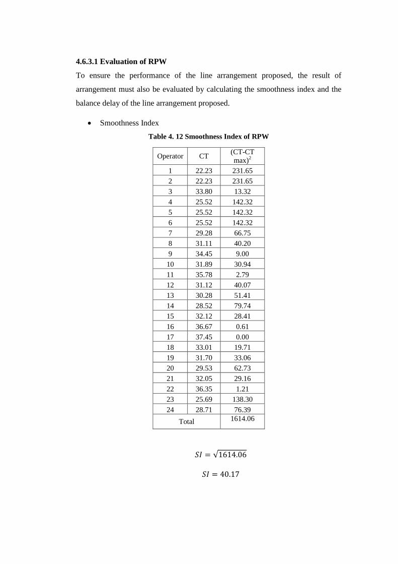
4.6.3.1 Evaluation of RPW
To ensure the performance of the line arrangement proposed, the result of
arrangement must also be evaluated by calculating the smoothness index and the
balance delay of the line arrangement proposed.
Smoothness Index
Table 4. 12 Smoothness Index of RPW
Operator CT (CT-CT
max)2
1 22.23 231.65
2 22.23 231.65
3 33.80 13.32
4 25.52 142.32
5 25.52 142.32
6 25.52 142.32
7 29.28 66.75
8 31.11 40.20
9 34.45 9.00
10 31.89 30.94
11 35.78 2.79
12 31.12 40.07
13 30.28 51.41
14 28.52 79.74
15 32.12 28.41
16 36.67 0.61
17 37.45 0.00
18 33.01 19.71
19 31.70 33.06
20 29.53 62.73
21 32.05 29.16
22 36.35 1.21
23 25.69 138.30
24 28.71 76.39
Total 1614.06
√
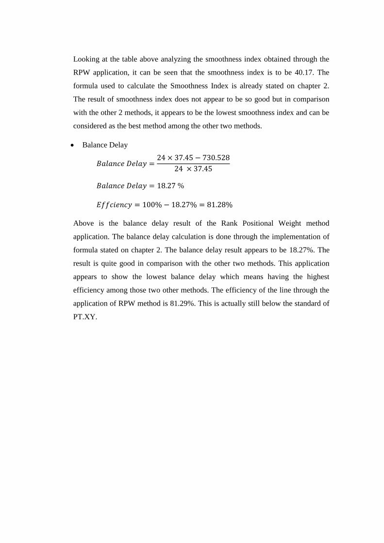
Looking at the table above analyzing the smoothness index obtained through the
RPW application, it can be seen that the smoothness index is to be 40.17. The
formula used to calculate the Smoothness Index is already stated on chapter 2.
The result of smoothness index does not appear to be so good but in comparison
with the other 2 methods, it appears to be the lowest smoothness index and can be
considered as the best method among the other two methods.
Balance Delay
%
Above is the balance delay result of the Rank Positional Weight method
application. The balance delay calculation is done through the implementation of
formula stated on chapter 2. The balance delay result appears to be 18.27%. The
result is quite good in comparison with the other two methods. This application
appears to show the lowest balance delay which means having the highest
efficiency among those two other methods. The efficiency of the line through the
application of RPW method is 81.29%. This is actually still below the standard of
PT.XY.

9
9
8
10 10
10 6
1,7
2,5
3,17
11,22
12,4
13,19
18,14
23,21
24,20
15
25,31,26
32,16
27,28
29,30
33
34,36
35
Conveyor
Figure 4. 10 Proposed Layout of Rank Position Weight
62

4.7 Comparison of Three Methods
After dealing with three methods to analyze the best result of line balancing, the
next thing is to compare all the result in terms of balance delay, efficiency, and
smoothness index
4.7.1 Balance Delay
Figure 4. 11 Balance Delay Comparison
Based on the table above, it is clear that the KWM method appears to be the
method with highest delay, thus the KWM is the worst in terms of Balance Delay.
Meanwhile, LCR and RPW method appears to show the best method in terms of
the delay. The LCR is still the lowest with a really slight different between these
two methods in terms of balance delay.
Figure 4. 12 Efficiency Comparison
0.00%
5.00%
10.00%
15.00%
20.00%
25.00%
30.00%
LCR KWM RPW
Pe
rce
nta
ge
Method
Balance Delay
Balance Delay
70.00%
72.00%
74.00%
76.00%
78.00%
80.00%
82.00%
LCR KWM RPW
Pe
rce
nta
ge
Method
Effieciency
Effieciency

Utilizing three different methods, the efficiency of those three methods have been
obtained. Looking at the efficiency result, the KWM again shows the lowest
efficiency. It all makes sense since the highest delay is at the KWM method. The
LCR and RPW method shows the same level of efficiency since this method have
low balance delay.
Figure 4. 13 Smoothness Index Comparison
The figure above shows the smoothness index comparison for Largest Candidate
Rule, Killbridge and Wester, and Rank Positional Weight Method. KWM again
shows the highest smoothness index while in this case, the lower smoothness
index, the better it is. LCR and RPW method again shows a slight different for
smoothness index. Using RPW method, the smoothness index appears to be the
best among those three methods as it shows the lowest value of smoothness index.
Looking at those three methods that have been applied; Largest Candidate Rule,
Killbridge and Wester Method, and Rank Position Weight, it is clear that the best
method to be applied is Rank Position Weight since it has the lowest balance
delay (can be considered the same with LCR) and also the lowest smoothness
index.
0
20
40
60
80
LCR KWM RPW
Smo
oth
ne
ss In
de
x P
oin
t
Method
Smoothness Index
Smoothness Index

4.8 Additional Action
The result of line balancing methods application do not really show a very good
yamazumi chart since some of the cycle time are still high. Thus, the additional
action is needed to reduce the cycle time in operation with high cycle time.
Figure 4. 14 Chosen Yamazumi Chart of RPW Application
Although it is found that the best method to be applied is Rank Positional Weight,
the room for improvement is still available there. It can be seen that some of the
cycle time is exceeding the takt time determined although it does not exceed
much. Let’s take a look at one example at operation 15 at workstation 17. The takt
cycle time at that work station is 37.45s meanwhile the takt time is 36. Not only
at work station 17, cycle time exceeding the takt time also happen at work station
16 and 22. Both do the operation 24 and 34,36. The next is focusing on reducing
cycle time at those both work stations.
1. Reducing Cycle time at operation 15 (Work Station 17)
Labor Data Sheet state that operation 15 is about attaching part to doll
together with the join head process. Here, looking at the precedence diagram
and the actual process, the join head process does not have to be done at work
station 17. It can be moved to next process at work station 20 with the cycle
time.
0
5
10
15
20
25
30
35
40
1 2 3 4 5 6 7 8 9 101112131415161718192021222324
Series1
Series2

There is an operation of attaching head to torso. Consulting with the IE
department, it can be moved to operation 14 at work station 14. At that work
station, the cycle time is still 28.52.
The time study is done to reduce the cycle time at work station 17. Below is
the CT of attaching head only.
Table 4. 13 Cycle time of attaching head
No CT
1 4.45
2 3.92
3 4.01
4 4.05
5 4.2
6 3.97
7 4.05
avg 4.09
Std dev 0.18
P Value 0.103
Min 3.92
Max 4.45
UCL 4.99
LCL 3.38
N’ 6.80
Based on the table, it can be concluded that the cycle time for head only 4.09.
Next is moving this operation to work station 14. After moving this operation,
the new time for this operation for work station 14 must be determined. Thus,
the time study must again be applied to determine the new time for this work
station. Below is the new time study result for work station 14.
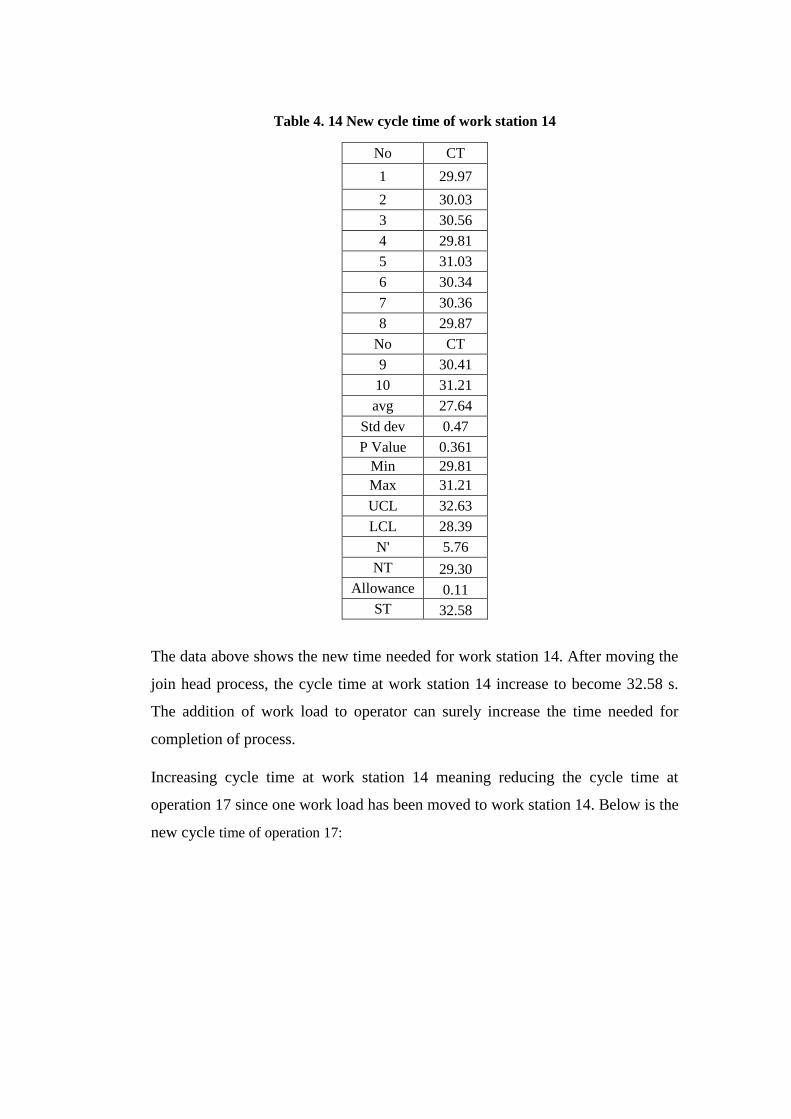
Table 4. 14 New cycle time of work station 14
No CT
1 29.97
2 30.03
3 30.56
4 29.81
5 31.03
6 30.34
7 30.36
8 29.87
No CT
9 30.41
10 31.21
avg 27.64
Std dev 0.47
P Value 0.361
Min 29.81
Max 31.21
UCL 32.63
LCL 28.39
N' 5.76
NT 29.30
Allowance 0.11
ST 32.58
The data above shows the new time needed for work station 14. After moving the
join head process, the cycle time at work station 14 increase to become 32.58 s.
The addition of work load to operator can surely increase the time needed for
completion of process.
Increasing cycle time at work station 14 meaning reducing the cycle time at
operation 17 since one work load has been moved to work station 14. Below is the
new cycle time of operation 17:

Table 4. 15 New cycle time for work station 17
No CT
1 26.46
2 27.04
3 27.04
4 28.31
5 27.61
6 27.31
7 27.43
8 28.09
9 27.21
10 27.41
avg 27.39
Std dev 0.53
P Value 0.281
Min 26.46
Max 28.31
UCL 29.90
LCL 24.87
N' 9.51
NT 29.58
Allowance 0.11
ST 32.90
Above is the cycle time of operation 17. It is clear that the cycle time has
successfully been reduced. The standard time is now become 32.90 seconds.
2. Adding Supporting Jig at Work Station 16
It can be seen that the current cycle time after the RPW method
implementation at work station 16 is still high. The processes itself are
assembly torso and tie down process. To reduce the cycle time at this work
station, additional jig is installed to ease the torso assembly process. Below is
the cycle time at works station 16 after installing the jig itself.

Table 4. 16 New cycle time for work station 16
No CT
1 27.075
2 28.12
3 27.15
4 27.15
5 28.09
6 27.32
7 27.41
8 28.21
9 26.97
10 27.03
avg 27.45
Std dev 0.49
P Value 0.872
Min 26.97
Max 28.21
UCL 29.69
LCL 25.49
N’ 9.26
NT 29.65
Allowance 0.11
ST 32.97
The cycle time at work station 16 has been reduced to become 32.97 since the jig
installment has made the operator easier during the assembly process since the
operator does not need to hold the torso by their hand anymore.
3. Replacing the Comb at Work Station 22 and 3
The operation at work station 22 is 33 which include trimming hair process. The
trimming process uses comb intently to do the doll hair treatment. Currently, the
comb used by the operator is rough and is not smooth when trimming process
using hair. Then, the new comb is given which is more smooth and leaner to make
the trimming process faster.

Table 4. 17 New cycle time for work station 22
No CT
1 26.125
2 27.02
3 25.05
4 26.12
5 25.98
6 26.54
7 25.63
8 26.42
9 26.01
10 25.42
avg 26.03
Std dev 0.57
P Value 0.890
Min 25.05
Max 27.02
UCL 28.72
LCL 23.35
N' 9.26
NT 28.11
Allowance 0.11
ST 31.26
Table above is the data of trimming process after changing with the new comb
with leaner design. It is way faster than before and it can be seen that the new
cycle time has been reduced to become 31.26 s.
Similar with work station 22, work station 3 also use comb as the tool. Although
the initial cycle time does not exceed the takt time, reducing the cycle time in this
work station can make the work distribution between each operator more balance.
Below is the new cycle time at work station 3.
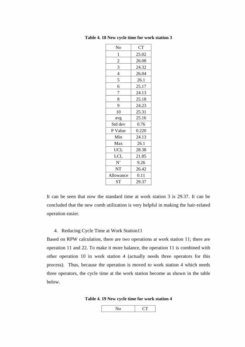
Table 4. 18 New cycle time for work station 3
No CT
1 25.02
2 26.08
3 24.32
4 26.04
5 26.1
6 25.17
7 24.13
8 25.18
9 24.23
10 25.31
avg 25.16
Std dev 0.76
P Value 0.220
Min 24.13
Max 26.1
UCL 28.38
LCL 21.85
N’ 9.26
NT 26.42
Allowance 0.11
ST 29.37
It can be seen that now the standard time at work station 3 is 29.37. It can be
concluded that the new comb utilization is very helpful in making the hair-related
operation easier.
4. Reducing Cycle Time at Work Station11
Based on RPW calculation, there are two operations at work station 11; there are
operation 11 and 22. To make it more balance, the operation 11 is combined with
other operation 10 in work station 4 (actually needs three operators for this
process). Thus, because the operation is moved to work station 4 which needs
three operators, the cycle time at the work station become as shown in the table
below.
Table 4. 19 New cycle time for work station 4
No CT

1 68.72
2 68.7
3 68.98
4 69.04
5 68.14
6 69.89
7 67.11
8 69.12
9 68.51
10 69.56
avg 68.78
Std dev 0.77
P Value 0.310
Min 67.11
Max 69.89
UCL 72.20
LCL 64.80
N' 9.26
NT 74.28
Allowance 0.11
ST 82.60
CT per Ops 27.53
Above is the new cycle time for work station 4.It has been increased since the
cycle time at work station 11 is reduced. The cycle time at Work station 11 only
left O-22 alone which is 29.78 s.
5. Reducing Cycle Time at Work station 9
Work station 9 consists of operation of cutting finish and dressing polybag. In this
operation, dressing method is introduced. Usually, the dressing is done after the
shoes are attached so the dress often sticks to the shoes. Now, the dressing process
first then the attaching shoes will be done later.
Table 4. 20 New cycle time for work station 9
No CT
1 24.55
2 25.21

3 24.03
4 24.21
5 25.43
6 23.98
7 24.55
8 25.24
9 23.94
10 24.45
avg 24.56
Std dev 0.56
P Value 0.175
Min 23.94
Max 25.43
UCL 27.10
LCL 22.27
N' 9.26
NT 26.52
Allowance 0.11
ST 29.49
Above is the cycle time at work station 9 after applying the new dressing method
and it is clear that the cycle time at work station can be reduced.
The cycle time in some work station have been improved and expected to lead to
the better result of efficiency. In conclusion, the new arrangement and the time
can be shown in the following table.
Table 4. 21 New cycle time for each work station
No Operation CT
Number of
Operator
CT of
Work
Station

0
5
10
15
20
25
30
35
40
1 2 3 4 5 6 7 8 9 101112131415161718192021
Cyc
le T
ime
(s)
Work Station
CT of Work Station
TT
1 O-9 44.46 2 22.23
2 O-8 29.37 1 29.37
3 O-10,O-11 82.59 3 27.53
4 O-6 29.28 1 29.28
5 O-1, O-7 31.11 1 31.11
6 O-2, O-5 29.49 1 29.49
7 O-3, O-17 31.888 1 31.888
8 O-22 29.78 1 29.78
9 O-12, O-4 31.12 1 31.12
10 O-13, O-19 30.28 1 30.28
11 O-18, O-14 32.58 1 32.58
12 O-23, O-21 32.12 1 32.12
13 O-24, O-20 32.97 1 32.97
14 O-15 32.9 1 32.9
15 O-25, O-31, O-26 33.01 1 33.01
16 O-32, O-16 31.7 1 31.7
17 O-27, O-28 29.53 1 29.53
18 O-29, O-30 32.05 1 32.05
19 O-33 31.26 1 31.26
20 O-34, O-36 25.69 1 25.69
21 O-35 28.71 1 28.71
Figure 4. 15 Improved Yamazumi Chart

4.9 Final Evaluation
As the additional action has been done to make the production process smoother,
then the final evaluation must be done to see the result obtained on terms of
Efficiency, balance delay, and smoothness index
Table 4. 22 Evaluation of Final Work Arrangement
No CT CT
Max-i
(CT
Max-i)2
1 22.23 10.8 116.21
2 22.23 10.8 116.21
3 29.37 3.6 13.25
4 27.51 5.5 30.25
5 27.51 5.5 30.25
6 27.51 5.5 30.25
7 29.28 3.7 13.91
8 31.11 1.9 3.61
9 29.49 3.5 12.39
10 31.888 1.1 1.26
11 29.78 3.2 10.43
12 31.12 1.9 3.57
13 30.28 2.7 7.45
14 32.58 0.4 0.18
15 32.12 0.9 0.79
16 32.97 0.0 0.00
17 32.9 0.1 0.01
18 33.01 0.0 0.00
19 31.7 1.3 1.72
20 29.53 3.5 12.11
21 32.05 1.0 0.92
22 31.26 1.8 3.06
23 25.69 7.3 53.58
24 28.71 4.3 18.49
Total 711.828 479.92
√
The calculation above shows that the smoothness has been improved to become
21.91. The next step is calculating the balance delay and efficiency as follows:
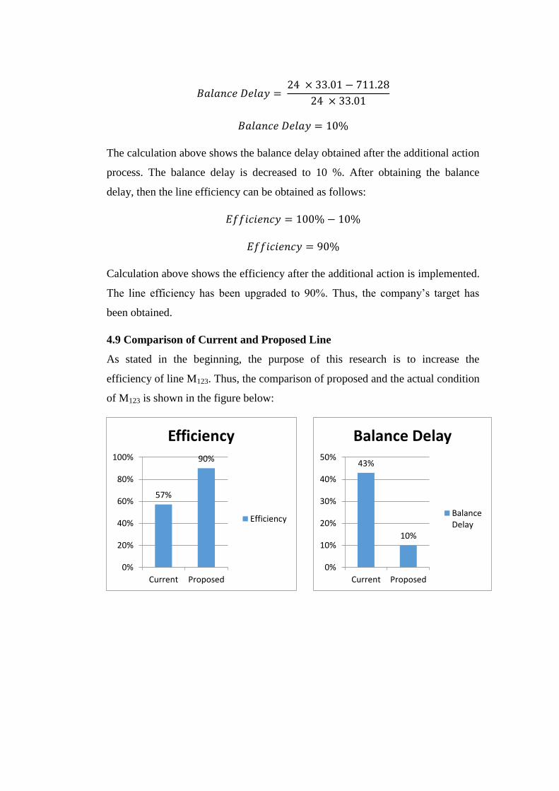
The calculation above shows the balance delay obtained after the additional action
process. The balance delay is decreased to 10 %. After obtaining the balance
delay, then the line efficiency can be obtained as follows:
Calculation above shows the efficiency after the additional action is implemented.
The line efficiency has been upgraded to 90%. Thus, the company’s target has
been obtained.
4.9 Comparison of Current and Proposed Line
As stated in the beginning, the purpose of this research is to increase the
efficiency of line M123. Thus, the comparison of proposed and the actual condition
of M123 is shown in the figure below:
57%
90%
0%
20%
40%
60%
80%
100%
Current Proposed
Efficiency
Efficiency
43%
10%
0%
10%
20%
30%
40%
50%
Current Proposed
Balance Delay
BalanceDelay

Figure 4. 16 Comparison between current and proposed line
Based on the graph shown in the figure above, it is clear that the proposed line is
much better than the previous one in terms of efficiency, balance delay, and
smoothness index. The efficiency increases from 57% to 90% and it has been
considered to fulfill the goal targeted by the company. The balance delay is
reduced up to 33% and smoothness index can be reduced.
Table 4. 23 The result of improvement
The improvement is not only by increasing efficiency, reducing balance delay,
and reducing smoothness index, it also includes the decrement number of
operator. Thus, the cost saving by applying this method can be calculated in the
table below.
Current Proposed Improvement
Efficiency 57% 93% 36%
Balance Delay 43% 7% 36%
Smoothness Index 65.86 21.91 43.95
65.86
21.91
0
10
20
30
40
50
60
70
Current Proposed
Smoothness Index
SmoothnessIndex

Table 4. 24 Cost comparison between actual and after improvement condition
Condition
# of
Opera
tor
Overtime
Monthly
operator
payment
Overtime Jig + Comb
investment Total
Current 34 68 110,840,000.00 1,360,000.00 - 112,200,000.00
Proposed 24 48 78,240,000.00 960,000.00 130,000.00 79,330,000.00
Total estimated saving per month
32,870,000.00
Note:
Minimun regional salary : IDR 3,260,000
Overtime wage : IDR 20,000 / hour
Jig price : IDR 100,000 / unit
Comb Price : IDR 15,000 / unit
It is obvious that the proposed line is much more profitable than the actual one.
The improvement condition still has to do the overtime since the cycle time
needed for the process is quiet high than the takt time must be adjusted too by
adding the number of working hour. In fact, it is still much profitable since the
number of operator can be decreased. Based on the cost saving analysis, the
company can save up to IDR 33,000,000 per month.
After calculating and analyzing all the data collected for this research, a new work
arrangement has been developed. The next chapter will provide the conclusion
and recommendation for future research.
CHAPTER V
CONCLUSION AND RECOMMENDATION
1.1 Conclusion
Based on the research that has been conducted, the conclusions are:
The root cause of having low efficiency is because the standard as the
guidance cannot accommodate the needs of actual condition and poor
work arrangement.
To increase the line efficiency, increasing the accuracy of each operation
is needed and continued by redesigning the work arrangement through the
line balancing method.
Based on the result, the research has achieved its objective as stated in the
beginning.
The line efficiency of M123 has increased to 32.89% from 57.11% to
90%
Number of operator in Line M123 can also be reduced by now only
utilizing 24 operators as the result of better efficiency.
1.2 Recommendation
Some of the production line at PT XY with the total number of operation exceed
35 usually experience low efficiency. The condition is worse when the toy
running in the production line may sometimes be changed based on the demand so
that re-arrangement is needed. Thus, the further research to increase the line
efficiency for the “complicated” toy is very beneficial.
REFERENCES
Elsayed, Elsayed A., and Boucher, T.O., Analysis and Control of Production
System, New York, Prentice Hall, 1985.
Hayter, A. Probability and Statistics for Engineers and Scientists 3rd Edition.,
Thomson.
Karger, D.W. & Bahya, F.H., Engineering Work Measurement 3rd Edition, New
York, The Industrial Press, 1977.
Niebel, B.W. & Freivalds, A., Niebel's Methods, Standards, and Work Design
12th Edition, New York, McGraw-Hill, 2003.
Pachghare, Vrittika V., Assembly Line Balancing Methods, Government College
of Engineering, 2012.
Sutalaksana, Iftikar Z., Anggawisastra, R. and Tjakraatmaja, J.H., Teknik
Perancangan Sistem Kerja, Bandung, ITB, 2006.
Taha, H., Operation Research: An Introduction 7th Edition, New Jersey, Prentice-
Hall, 2003.
Walpole, R.E., Myers, R.H., Myers, S.L. & Ye, K., Probability and Statistic for
Engineers and Scientists 7th Edition, New Jersey, Prentice-Hall, 2002.
Wignjosoebroto, S., Ergonomi, Studi Gerak dan Waktu. Surabaya, Guna Widya,
2000.

Minkjan, OBIEE Creating a Yamazumi Graph, 2010. Retrieved January 02, 2016,
from http://knowledge.ciber.nl/weblog/?p=183
Till, W., Tact Time, 2010. Retrieved November 12, 2015, from Kaizen Today:
http://kaizentoday.com/page/Pages/Tact-Time.aspx