Wright State University Wright State University

CORE Scholar CORE Scholar

Browse all Theses and Dissertations Theses and Dissertations

2017

Incorporating Passive Compliance for Reduced Motor Loading Incorporating Passive Compliance for Reduced Motor Loading

During Legged Walking During Legged Walking

Akhil Sai Pabbu Wright State University

Follow this and additional works at: https://corescholar.libraries.wright.edu/etd_all

Part of the Electrical and Computer Engineering Commons

Repository Citation Repository Citation Pabbu, Akhil Sai, "Incorporating Passive Compliance for Reduced Motor Loading During Legged Walking" (2017). Browse all Theses and Dissertations. 1790. https://corescholar.libraries.wright.edu/etd_all/1790

This Thesis is brought to you for free and open access by the Theses and Dissertations at CORE Scholar. It has been accepted for inclusion in Browse all Theses and Dissertations by an authorized administrator of CORE Scholar. For more information, please contact library-corescholar@wright.edu.

INCORPORATING PASSIVE COMPLIANCE FOR REDUCE

MOTOR LOADING DURING LEGGED WALKING

A thesis submitted in partial fulfillment of the

requirements for the degree of

Master of Science in Electrical Engineering

By

AKHIL SAI PABBU B.Tech, Jawaharlal Nehru Technological University, India, 2015

2017

Wright State University

WRIGHT STATE UNIVERSITY

GRADUATE SCHOOL

July 19, 2017

I HEREBY RECOMMEND THAT THE THESIS PREPARED UNDER MY SUPERVISION BY Akhil

Sai Pabbu ENTITLED ‘Incorporating Passive Compliance for Reduce Motor Loading

During Legged Walking’ BE ACCEPTED IN PARTIAL FULFILLMENT OF THE

REQUIREMENTS FOR THE DEGREE OF Master of Science in Electrical Engineering.

AAAAAAAAAAAAAAAAAAAA Luther R. Palmer III, Ph.D.

Thesis Director

AAAAAAAAAAAAAAAAAAAA

Brian Rigling, Ph.D.

Chair, Electrical Engineering

Committee on Final Examination

AAAAAAAAAAAAAAAAAA A Luther R. Palmer III, Ph.D.

AAAAAAAAAAAAAAAAAAA A Zach Fuchs, Ph.D.

AAAAAAAAAAAAAA AAAAAA Xiaodong (Frank) Zhang, Ph.D.

AAAAAAAAAA AAAAAAAAA Robert E. W. Fyffe, Ph.D.

Vice President for Research and

Dean of the Graduate School

ABSTRACT

Pabbu, Akhil Sai. M.S.E.E. DEPARTMENT OF ELECTRICAL ENGINEERING,

Wright State University 2017. ‘Incorporating Passive Compliance for Reduced Motor

Loading During Legged Walking’

For purposes of travelling on all-terrains surfaces that are both uneven and discontinuous, legged

robots have upper-hand over wheeled and tracked vehicles. The robot used in this thesis is

a simulated hexapod with 3 degrees of freedom per leg. The main aim is to reduce the

energy consumption of the system during walking by attaching a passive linear spring to each leg

which will aid the motors and reduce the torque required while walking. Firstly, the ideal

stiffness and location or the coordinates for mounting the spring is found out using gradient

based algorithm called ‘Simultaneous Perturbation and Stochastic Approximation

Algorithm’ (SPSA) on a flat terrain using data from a single walking step. Motor load is

approximated by computing the torque impulse, which is the summation of the absolute value of

the torque output for each joint during walking. Once the ideal spring and mount is found, the

motor loading of the robot with the spring attached is observed and compared on three different

terrains with the original loading without the spring. The analysis is made on a single middle

leg of the robot, which is known to support the highest load when the alternating tripod gait is

used. The obtained spring and mounting locations are applied to other legs to compute the overall

energy savings of the system. Through this work, the torque impulse was decreased by 14 % on

uneven terrain.

iii

Keywords: Legged robots, Energy optimization in legged robots, Optimization using SPSA,

Gradient based optimization, Spring placement on a hexapod, Energy cost, Torque

distribution.

vi

Table of Contents:

1. Introduction

1.1. Legged Walking 1

1.2. Hexapod Gaits 2

1.2.1. Tripod gaits 3

1.2.2. Wave gait 4

1.2.3. Ripple gait 41.3. Hexapod Stride 5

1.3.1. Stance Phase 6

1.3.2. Swing Phase 6

1.3.3. Stride Period 7

1.4. Other Hexapod Systems 7

1.4.1. RHex 8

1.4.2. Lauron V 8

1.5. Contribution 10

2. Approach

2.1. Spring Attachment 11

2.2. Simultaneous Perturbation and Stochastic Approximation Algorithm (SPSA) 17

2.3. RoboDynamichs 223. Results

3.1. SPSA Results 253.2. Step Results 29

4. Future Work 355. References 37

v

List of Figures

1.1. Figure explaining different parts of the robot leg 1

1.2. Picture of Hexapod Robot discussed in this thesis 2

1.3. Figure explaining the leg numbering of the robot 3

1.4. Figure shows different gait patterns 5

1.5. Figure shows the stance phase of the leg during a stride 6

1.6. Figure shows the swing phase of the leg during a stride 7

1.7. RHex robot 8

1.8. DynaRoach Robot 8

1.9. Lauron V 9

1.10. Hexapod Robot discussed in this thesis 9

2.1. [1a] Torque exerted by the motor to support body weight of the robot 11

2.2. [1b] Torque required to lift the leg up in the air during Swing phase 11

2.3. [2a] Desired torque to support the body of the robot 12

2.4. [2b] Desired torque to lift the leg during Swing phase 12

2.5. [3a] Mounting position of the Torsional Spring 12

2.6. [3b] Torque applied by the torsional spring during Stance phase 12

2.7. [4a] Total torque applied by spring and motor during Stance phase 13

2.8. [4b] Total torque applied by the motor to lift the leg during Swing phase 13

2.9. [5a] Placement of the linear spring 13

2.10. [5b] Total Torque applied by spring and motor 13

2.11. [6a] Torque applied by the motor at Zero-torque angle 14

2.12. [6b] Torque required by the motor to lift the leg and support the opposing spring

torque 14

2.13. [7a] Figure showing the Co-ordinate system of the search space used for SPSA

algorithm 15

2.14. [7b] Spring and leg angles with respect to search space 15

vi

2.15. Plot of the cost with respect to number of iterations used in this thesis 19

2.16. Plot of cost with respect to iterations after adjusting the parameters 21

2.17. Figure which shows the user interface of the RoboDynamics tool 22

2.18. figure which shows the random terrain 23

2.19. figure that shows step terrain 24

3.1. 3-D response surface BX = 0, and cost versus AX, AY on X and Y axis

respectively and BY on Z axis 26

3.2. 3-D response surface at BX = 1cm, Cost vs BX, AX, AY 27

3.3. 3-D response surface at BX = -1cm, Cost vs BX, AX, AY 27

3.4. 3-D response surface at BX = 2cm, Cost vs BX, AX, AY 28

3.5.Step analysis of the results obtained from SPSA 29

3.6. Zero torque angle = -41.29⁰ 30

3.7. Extension of the Spring with respect to time 30

3.8. Plots of various torques with respect to time 30

3.9. Magnitude plot of various torques along with the contact vector 31

3.10. Integral of all the torques 31

3.11. Analysis of different factors, while robot walks 4 steps 32

3.12. Subplot of Magnitude of various torques along with the contact vector during all 4

steps 32

3.13. Plot of Magnitude of various torque along with contact vector during single step.

32

3.14. Analysis of different factors on step up terrain for 4 steps 33

3.15. Analysis of the various factor on random terrain for 4 steps Initial Torque:

2555.88 N.m, New Torque: 2266.85 N.m, Efficiency: 11% 34

vii

Chapter 1: Introduction

1.1 Legged Walking:

There are many forms of locomotion available for robotic system, one of which is

legged walking, others being on wheels, hovering etc. This thesis report consists of a study

of how legged walking can be improved on a hexapod system by reducing of energy

consumed while walking.

A legged hexapod has a general construction of six legs of three segments each:

coxa, femur, and tibia. For a hexapod to walk with stability, the angle and position of all

the legs and their parts need to be controlled according to a coordinated gait pattern.

;

Figure 1.1: Figure explaining different parts of the robot leg

Legged walking has a significant advantage when the robot needs to navigate on a

rough terrain. The lift-and-place method used by the legs of the robot can make it robust to

1

unwanted disturbance as they do not need continuous contact with the ground. This

has attracted considerable attention in the past decade. There are several other benefits of

legged walking: efficient in maintaining stability with three of more legs, usage of gaits for

locomotion so the speed of locomotion can be varied easily, legs do less damage to the

terrain than tracks and wheels. Also, the height of the robot can be changed according to

the constraints if the leg joints are built to have sufficient degrees of freedom.

Primary disadvantages of legged robots are the complexity of the systems and energy

usage. This thesis seeks to address the latter concern by incorporating passive compliance

in each leg.

Figure 1.2: Picture of Hexapod Robot discussed in this thesis

1.2 Hexapod gaits:

During the walking of a legged robot, there is a crucial problem of generation and

control of the sequence of placing and lifting the legs such that at any instant, the body

2

should be stable and capable of moving from one position to another. The generation and

sequence of such leg motion is called Gait. Gaits are repeated periodically on a robot for

successful locomotion from one point to another.

The hexapod robot has six legs for locomotion, at least three of which need to be

on the ground at any point of time to ensure stable locomotion. There are three main gaits

used by a hexapod robot: wave gait, ripple gait and tripod gait; each ensuring system

stability always.

Figure 1.3: Figure explaining the leg numbering of the robot

1.2.1 Tripod gait:

The walking stride of the tripod gait in a hexapod robot consists of two individual

steps. At any instance, at least three legs of the robot stand on the ground providing support

and force to push the body forward while the other three legs swing forward to take

the stance position. Considering the legs of the robot are numbered as shown in Figure

1.3, legs 1, 3, and 5 begin in a stance (on the ground) position and legs 2, 4 and 6 swing

forward in flight. As the legs 2, 4, and 6 touch the ground, they change to stance position

while legs 1, 3, and 5 swing forward in flight. Thus the hexapod moves forward in a

cycle of two simple steps in tripod gait. The foot fall pattern of Tripod gait is shown

in Figure 1.4

3

1.2.2 Wave gait:

The walking mechanism of the wave gait in a hexapod robot consists of six steps.

At any instance, at least five legs of the robot stand on the ground providing support and

force to push the body forward while the other leg swings forward to take the stance

position. Considering the legs of the robot are numbers as shown in Figure 1.3, legs 1, 2,

4, 5 and 6 begin in a stance position and leg 3 swings forward. Then, leg 2 swings

forward while the others are in the stance phase. Then, leg 1 swings forward, followed by

legs 6, 5 and 4 while the other legs are in stance phase for each step. Thus, to complete

one cycle of a Wave gait, six legs take six individual steps each. The foot fall pattern of

Wave gait is shown in Figure 1.4

1.2.3 Ripple gait:

The walking mechanism of the ripple gait in a hexapod robot consists of six steps.

At any instance, at least four legs of the robot stand on the ground providing support and

force to push the body forward while the other two legs swing forward to take the stance

position. Considering the legs of the robot are numbers as shown in Figure 1.3, legs 1, 2, 5

and 6 begin in a stance position and legs 3 and 4 swings forward. While leg 4 is still in

swing position leg 2 begin to swing. Leg 6 start swinging as soon as leg 4 touches down.

This pattern is followed by the legs to complete the gait. Thus, to complete one cycle of a

Ripple gait, it takes 3 steps. The foot fall pattern of Ripple gait is shown in Figure 1.4

4

Figure 1.4: Figure shows different gait patterns

1.3 Hexapod Stride

While walking, each leg of the hexapod repetitively goes through two phases:

stance and swing. These two phases together complete one cycle of the hexapod stride. The

time periods for which the legs stay in stance phase and swing phase are called stance

period and swing period, respectively. These are controlled by an aspect called duty factor,

which is the ratio of the stance period of the leg to its total stride period. For example, if

the legs move in stance and swing phases for equal amount of times, that is, if the stance

period is equal to the swing period, the duty factor of the gait is computed to be 0.5. If the

leg is in stance for 75% of the entire stride, the duty factor is 0.75. The duty factor

ranges

5

between 0 and 1, and it is the same value for all the legs of the hexapod while the system

moves in a gait.

1.3.1 Stance period:

This is the time period for which the leg of the hexapod is in contact with

the ground. During locomotion, the legs that are in the stance phase help to provide

stability to the system while pushing the body forward. Together, they form a support

polygon that is used to calculate the stability margin of the body in its current position.

Figure 1.5: Figure shows the stance phase of the leg during a stride

1.3.2 Swing period:

This is the time-period for which the leg of the hexapod is swinging forward.

During locomotion, the swing period of the legs is used to bring the legs forward by lifting

them off the ground and moving them ahead of the leg-body joint so as to take the stance

phase at the beginning of the next cycle.

6

Figure 1.6: Figure shows the swing phase of the leg during a stride

1.3.3 Stride Period:

This is the total time period that constitutes a swing phase and stance phase. That

is, the leg completes a full 360-degree rotation at the leg-body joint in one stride period.

The stride period of the body is decided based on the velocity with which the system is

moving forward. The duty factor is then used to compute the swing and stance periods.

All the legs on the system operate using the same values for each of the above time periods.

Thus, the gait of the hexapod is changes either by varying the body velocity, or the duty

factor. This report mainly details the work based on a tripod gait using a 75% duty factor.

1.4 Other Hexapod Robots:

The more legs that a system has, the less challenging it is to maintain stability.

Specifically, hexapods possess greater static stability both while standing and while

walking over 4-legged robots. Most of these hexapod robots are inspired from biological

7

species, but are not intended to explicitly mimic these systems. A few of these hexapod

robots are described below.

1.4.1 RHex:

This is a design inspired from biological species. It does not have a multi-joint leg

and also was the inspiration for the miniature robot called The DynaRoACH robot which

is only 10 cm in length and weighs 24 grams. This system can travel 14 body lengths per

second [3].

Figure 1.7: RHex robot Figure 1.8: DynaRoach Robot

This design is described as under actuated, as there are passive joints that are not explicitly

controlled. As there is not much joint movements or complex controlling. Due to its small

size, the DynaRoach robot’s legs are made out of polyelastic materials which makes it

easier to tune the stiffness of its legs. By adjusting the stiffness, the stability of the robot

can be maintained [4].

1.4.2 Lauron V:

Lauron is a biologically-inspired robot which mimics the walking behavior of the

stick insect Carausius Morosus. The research on Lauron started in early 1990s and led to

the development of Lauron I which is in contrast with the present Lauron V. Lauron V has

the artificial neural network. The name of the robot LAURON which actually stands for

LAUf Roboter Neuronal Gesteuert meaning neural controlled walking robot [5].

8

This robot was actually developed to study and realize the statically stable walking in rough

terrain. Due to its flexible behavior walking control, this robot can adopt itself to different

terrains. And, its robust design and multiple joint legs which gives more degrees of freedom

helps it to maintain stable locomotion under various circumstances [6].

Figure 1.9: Lauron V

The robot used in this thesis is custom built and is rectangular as shown in figure

below. By using the spring, the motor load of the dominant joint during walking is

optimized to 28%. These results are obtained by using the leg #2 on a flat terrain but by

extrapolating these results to other legs, the efficiency can be increased. The same robot is

then tested on different terrains and the results are compared among these terrains.

Figure 1.10: Hexapod Robot discussed in this thesis

9

1.5 Contribution:

There have been various methods to optimize the energy of a hexapod robot. Some

of them have adopted for an efficient body shape and design, few have adopted for a

different leg design and few other choose a design which gives them a better and efficient

zero torque angle.

In same way, this thesis consists of a different approach of using springs to assist

the motors and reduce the total torque required by them for walking. As the data used in

all the simulations to get the lowest cost is based on a robot which is already build, this is

not the most efficient way of placing the spring as the priority here has been given to an

easy design than getting to a spring placement that gives lowest cost. By making few

changes to the SPSA algorithm used in this thesis this concept can be adopted to optimize

the energy consumption of any state of the art hexapod robot that are present.

The big picture will be adopting this concept on robots which are not just hexapods,

but also bipeds, quadrupeds and other leg arrangements.

10

Chapter 2: Approach

2.1 Spring Attachment:

This section is the most important part of this thesis due to following factors

1. It helps to understand how various torques act on the leg of the robot.

2. It shows how the spring is mounted on the robot

3. It explains the search space around the robot used for SPSA algorithm

4. It shows the working of different types of springs

Points to be noted:

color indicates the torque applied by the motor

color indicates the torque applied by the spring or the spring force

Assume that the duty cycle for this stride period is 75%

Figure 2.1: [1a] Torque exerted by the

motor to support body weight of the

robot

Figure 2.2: [1b] Torque required to lift

the leg up in the air during Swing

phase

11

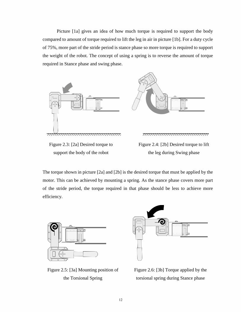
Picture [1a] gives an idea of how much torque is required to support the body

compared to amount of torque required to lift the leg in air in picture [1b]. For a duty cycle

of 75%, more part of the stride period is stance phase so more torque is required to support

the weight of the robot. The concept of using a spring is to reverse the amount of torque

required in Stance phase and swing phase.

Figure 2.3: [2a] Desired torque to

support the body of the robot

Figure 2.4: [2b] Desired torque to lift

the leg during Swing phase

The torque shown in picture [2a] and [2b] is the desired torque that must be applied by the

motor. This can be achieved by mounting a spring. As the stance phase covers more part

of the stride period, the torque required in that phase should be less to achieve more

efficiency.

Figure 2.5: [3a] Mounting position of

the Torsional Spring

Figure 2.6: [3b] Torque applied by the

torsional spring during Stance phase

12

One way of achieving this efficiency is by mounting the spring as shown in picture [3a].

So that it applies a torque as shown in picture [3b] there by reducing the torque required

during stance phase.

Figure 2.7: [4a] Total torque applied by

spring and motor during Stance phase

Figure 2.8: [4b] Total torque applied by

the motor to lift the leg during Swing

phase

Total torque applied by the spring and motor to support the weight of the robot is shown in

picture [4a] which is similar to the desired one. But when it comes to picture [4b], the

torque required to lift the leg and oppose the spring torque is very high, more than the

desired. This type of spring will hurt the system than helping it.

Figure 2.9: [5a] Placement of the linear

spring

Figure 2.10: [5b] Total Torque applied

by spring and motor

13

Due to the failure of torsional spring, a linear spring is mounted as shown in picture [5a].

This spring is expected to overcome the drawback of the torsional spring. Similar to the

torsional spring, the linear spring also supports the weight of the robot as shown in picture

[5b].

Figure 2.11: [6a] Torque applied by the

motor at Zero-torque angle

Figure 2.12: [6b] Torque required by

the motor to lift the leg and support the

opposing spring torque

But one point which cannot be possible in torsional spring is the zero-torque angle. A

position in which the two anchors of the spring, the axis on which the leg rotates all stay in

a line. At this point, the spring force is cancelled out by the axis. Therefore, only force

acting on the leg is the torque applied by the motor. This position is explained through

picture [6a]. Even at an angle which is greater than the zero-torque angle, the force applied

by the spring will be less as it the rectangular component of the actual force. Due to which

the total force applied by the motor to support the weight of the leg and counter the torque

applied by the spring is very low. This case is shown in picture [6b].

14

Figure 2.13: [7a] Figure showing the

Co-ordinate system of the search space

used for SPSA algorithm

Figure 2.14: [7b] Spring and leg angles

with respect to search space

Picture [7a] shows the direction of X-axis and Y-axis for the search space used in SPSA

algorithm. ‘A’ and ‘B’ are the two ends of the spring or the anchor points of the spring.

Point ‘A’ is the proximal anchor and point ‘B’ is the distal anchor. All the notations in the

MATLAB code and SPSA are based on ‘A’ and ‘B’ points. Picture [7b] is used as the

reference for the terminology for the equations used to calculate all the parameters in the

user built function getSpringtorque().

Equations:

The initial spring length, d0, is computed at the mounting location of the spring as

𝑑0 = √(𝑎𝑥 − 𝑏𝑥,𝑖𝑛𝑖𝑡)2

+ (𝑎𝑦 − 𝑏𝑦,𝑖𝑛𝑖𝑡)2

The distal anchor position, b, moves as the leg moves, and is computed as a rotation

about the leg angle, θleg by

𝑏 = [cos (𝜃𝑙𝑒𝑔) sin (𝜃𝑙𝑒𝑔)

−sin (𝜃𝑙𝑒𝑔) cos (𝜃𝑙𝑒𝑔)] [

𝑏𝑥,𝑖𝑛𝑖𝑡

𝑏𝑦,𝑖𝑛𝑖𝑡]

15

Note that the proximal anchor position does not change. The current spring length, d, is

computed by

𝑑 = √(𝑎𝑥 − 𝑏𝑥)2 + (𝑎𝑦 − 𝑏𝑦)2

The scalar spring force is computed using the spring constant, k, as

𝑓𝑠𝑝𝑟𝑖𝑛𝑔 = 𝑘(𝑑 − 𝑑0)

The direction of the spring force is

𝜃𝑠𝑝𝑟𝑖𝑛𝑔 = 𝑎𝑡𝑎𝑛2(𝑏𝑦 − 𝑎𝑦, 𝑏𝑥 − 𝑎𝑥)

and the spring force vector is computed by

𝑓𝑠𝑝𝑟𝑖𝑛𝑔𝑥 = 𝑓𝑠𝑝𝑟𝑖𝑛𝑔cos (𝜃𝑠𝑝𝑟𝑖𝑛𝑔), and

𝑓𝑠𝑝𝑟𝑖𝑛𝑔𝑦

= 𝑓𝑠𝑝𝑟𝑖𝑛𝑔sin (𝜃𝑠𝑝𝑟𝑖𝑛𝑔)

Finally, the spring-generated torque is the cross product of the b vector and the spring

force vector:

16

𝜏𝑠𝑝𝑟𝑖𝑛𝑔 = 𝑏 𝑥 𝑓𝑠𝑝𝑟𝑖𝑛𝑔 = 𝑏𝑥𝑓𝑦 + 𝑏𝑦𝑓𝑥

After mounting the spring, the equation for total torque can be given by

𝐼𝜏 = ∑|𝜏𝑚𝑜𝑡𝑜𝑟 + 𝜏𝑠𝑝𝑟𝑖𝑛𝑔|

where 𝜏𝑚𝑜𝑡𝑜𝑟 is the torque provided by the motor and 𝜏𝑠𝑝𝑟𝑖𝑛𝑔 is the torque provided by the

spring.

2.2 SPSA:

The Simultaneous Perturbation Stochastic Approximation Algorithm (SPSA) is an

efficient gradient based algorithm used to find the minimum local cost for optimization

over a set of cost functions (response surfaces). The details of the algorithm are as given

below.

For instance, assume that there is a 2-D search space which need to be optimized.

Therefor p = 2, where ‘p’ is the dimension of the search space. The cost ‘J’ is a function of

‘θ’ where size of ‘θ’ depends on value of ‘p’. In this case,

𝜃 = [𝜃1 𝜃2]

where size of ‘θ’ and ‘c’ is [1 x p]. The accuracy of the system depends on number of

iterations ‘j’, value of ‘𝜆’ which is the ‘step size’ and the value of ‘c’ which is the ‘viewing

distance’. Guidelines for choosing the values for ‘𝜆’ and ‘c’ are given in the next section.

Once we chose values for ‘𝜆’, ‘c’ and initial ‘θ’ i.e. θj=1, the SPSA calculates the

gradient for those values by

𝑔𝑖(𝜃(𝑗), 𝑗) = 𝐽𝑛(𝜃(𝑗)) + 𝑐𝑗𝛥(𝑗)) − 𝐽𝑛(𝜃(𝑗) − 𝑐𝑗𝛥(𝑗))

2𝑐𝑗𝛥𝑖(𝑗)

where cj > 0 for all j and

𝛥(𝑗) = [

𝛥1(𝑗)⋮

𝛥𝑝(𝑗)]

17

is a random perturbation vector. The components of the vector Δ(j) should be

independently generated from a zero-mean probability distribution and one theoretically

valid choice is to use a Bernoulli ±1 distribution for each ±1 outcome. In this way, the

𝜃(𝑗) ± 𝑐𝑗𝛥(𝑗) lie in a known bounded region. Note that if p =2 , then the Δ(j) are the corners

of a unit square so for each j

𝛥(𝑗) ∈ {[11

] , [1

−1] , [

−11

] , [−1−1

]}

In general, there are 2p possible 𝛥(𝑗)values.

After the gradient is calculated, the ‘θ’ value is updated as follows

𝜃(𝑗 + 1) = 𝜃(𝑗) − 𝜆𝑗𝑔(𝜃(𝑗), 𝑗)

Where 𝑔(𝜃(𝑗), 𝑗) 𝜖 𝔑𝑝 is an estimate of ∇J(θ(j)) at θ(j).

In this thesis, SPSA is used to optimize the total torque required by the motor for

walking. This is done with the help of a spring placed between the body and the Coxa of

the leg. The total torque changes with the position of the spring. In a two-dimensional

coordinate system, the position of the spring can be described using four values: (x, y) of

the distal joint, (x, y) of the proximal joint. Thus, the response function used in this thesis

is a 4-D search space.

18

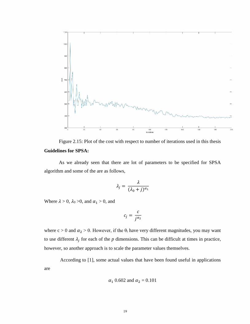
Figure 2.15: Plot of the cost with respect to number of iterations used in this thesis

Guidelines for SPSA:

As we already seen that there are lot of parameters to be specified for SPSA

algorithm and some of the are as follows,

𝜆𝑗 = 𝜆

(𝜆0 + 𝑗)𝛼1

Where 𝜆 > 0, 𝜆0 >0, and 𝛼1 > 0, and

𝑐𝑗 = 𝑐

𝑗𝛼2

where c > 0 and 𝛼2 > 0. However, if the θi have very different magnitudes, you may want

to use different 𝜆𝑗 for each of the p dimensions. This can be difficult at times in practice,

however, so another approach is to scale the parameter values themselves.

According to [1], some actual values that have been found useful in applications

are

𝛼1 0.602 and 𝛼2 = 0.101

19

Which are effectively the lowest allowable ones that satisfy theoretical conditions.

Step by Step working of SPSA:

1. All the values for 𝜆, c, 𝛼1, 𝛼2 and number of steps are chosen.

2. A random initial value for 𝜃 is chosen, the thetaplus and thetaminus values for this

particular 𝜃 are calculated at a distance of ‘c’ along with the respective costs.

3. Once the costs are known, the algorithm tries to move towards the lower cost with

a step size of 𝜆.

4. Then the values of 𝜆 𝑎𝑛𝑑 𝑐 are reduced. In other words, new values of 𝜆 𝑎𝑛𝑑 𝑐 are

calculated based on the values of 𝛼1, 𝛼2

5. All these steps repeat until the values of 𝜆 𝑎𝑛𝑑 𝑐 become so small that the algorithm

will not be able to move any further down the gradient.

Changes made to the normal SPSA algorithm:

All the steps explained above are for normal SPSA algorithm. But in this case the

algorithm is a 4-D search space with lot of limitations. In this thesis, the priority was given

for easy design of the robot than perfect energy optimization. This helps to mount the spring

on the robot without additional work done on it or any other hassle.

The changes that were made to the search algorithm are as follows:

The equation for the final cost is given by

𝑐𝑜𝑠𝑡𝑓𝑖𝑛𝑎𝑙 = 𝐼𝜏 + 𝛼1 ∗ max(−𝑝𝑟𝑒𝑙𝑜𝑎𝑑, 0) + 𝛼2 ∗ max((𝑚𝑎𝑥𝑙 − 𝑙𝑚𝑎𝑥), 0) + 𝛼3

∗ 𝑎𝑏𝑠(𝑎𝑦) + 𝛼4 ∗ 𝑎𝑏𝑠(𝑏𝑥)

where ′𝑚𝑎𝑥𝑙′ is the maximum allowable spring length; ′𝑙𝑚𝑎𝑥′ is the maximum length the

spring extends during the stride. ′𝑝𝑟𝑒𝑙𝑜𝑎𝑑′ is the extension on the spring on its mounting

position and 𝐼𝜏 is given in section 2.1

1. Three extra parameters are added to the cost obtained from the impulsefunction().

They are ‘preload’, ‘maximum allowable spring length’ and ‘distance of AX and

BX from origin’

20

2. It is adjusted in such a way that, if preload is a negative the cost increases. To put

it in better words, if the initial spring length is more than the preload we cannot

install the spring.

3. Same goes with ‘maximum allowable spring length’. If the spring extends more

than actual physical extendable limit of the spring in the simulation, the system

breaks the spring, which is not feasible. If this value is negative the cost increases.

4. The parameter is used in order to make sure that one end of the spring stays on the

leg rather going sideways from the leg. And the other end stays on the body of the

robot rather going downwards from the body of the robot. More the distance from

the origin, more is the cost.

5. The magnitude in which these three parameters increase in the cost is controlled by

three different gains called ‘gsin1, gain2 and gain3’.

Figure 2.16: Plot of cost with respect to iterations after adjusting the parameters

21

2.3 RoboDynamics:

RoboDynamics is tool which helps us to simulate the physical effects on any kind

of machine. This tool has flexibility to program which ever terrain needed. In this case,

Random terrain, Flat terrain and Step terrain. This system samples the data every

millisecond (every thousandth of a sec). This tool also offers various options to export the

data that is required according to use. Few of the examples in this case are contact, torque

and angle of the leg during a complete step.

Figure 2.18: Figure which shows the user interface of the RoboDynamics tool

: This button is used to start the simulation

: This button is used to pause the simulation in middle

: This button is used to stop the simulation. Once you hit this button all the data is

exported

22

: This button is used to turn on the simulation. Without this button we cannot start

the simulation.

: This slider is used to seek forward or reverse with respect to time of the

simulation.

There are also various other options like Loaded objects and configuration which

is used to define the robot’s body and properties. If there are any other objects to be placed

on the environment their properties are defined in this option itself.

To define the properties of the environment, say type of terrain, color of the terrain,

height and depth of the terrain etc. can be defined using the environment option. The

playback tab provides us with various options like location for the storage of the data,

different types of parameters to be exported in the form of data etc.

The figures demonstrate what all terrain are used and how they look

Figure 2.19: figure which shows the random terrain

23

Figure 2.20: figure that shows step terrain

24

Chapter 3: Results

After using SPSA with 10 random initial points, and each point tested for 5 times,

the obtained results for mounting position which is optimized both for energy and design

is

AX = -0.0091m AY = -0.0079m

BX = -0.0066m BY = -0.0600m

Spring Stiffness = 1402.7659N/m Initial Length = 0.0508m

This spring can be found at www.mccmaster.com with a part number 9654K365

3.1 SPSA Results

When SPSA algorithm was performed on 2-D and 3-D search space, the results

were accurate. There were no complications. But when the dimensions of the search space

started increasing the results were not satisfactory. In order to figure out what makes the

SPSA fail to work, the response surface of the impulsefunction() is plotted. But as our

imagination is limited to three dimensions, one of the dimension is made constant and the

response surface or the cost of the impulse function is plotted with respect to AX, AY, BY

keeping BX constant. In this way, it is possible to look at the 3-D space of the response

surface. The cost is defined according to color.

25

Figure 3.1: 3-D response surface BX = 0, and cost versus AX,AY on X and Y axis

respectively and BY on Z axis

In the above figure, the range of the cost is given by a color bar on the right, where

blue defines the lowest cost and yellow defines the highest cost. As it is clearly seen that

there is a shelf kind of area in the plot. This shelf has the lowest gradient. Due to which the

SPSA takes forever to reach the lowest point.

Let’s say that the number iterations are 400, and It takes all 400 steps for the

algorithm to reach some random point on the shelf (as SPSA is a random algorithm) then

to reach to lowest point from that position it might even need more than a million steps. It

is clearly seen in the system that there is minimum point, which could be the solution for

this search (point with the lowest cost) which could be reached by more computations but

at what cost? Even if we reach to the lowest point it might not be efficient, computational

wise. So we resorted to the anchor points on the shelf which provide a cost that is in a range

of 10% or 5% of the lowest point. If this is the case with three dimensions, then this

ambiguity will continue to four dimensions too. Hence, we cannot get the same point or

points that are close to the minimum all the time. This is where SPSA fails to get the exact

solution (which is a primary requirement for the algorithm to be considered successful).

The response surfaces of the cost with different BX values are also shown below.

26

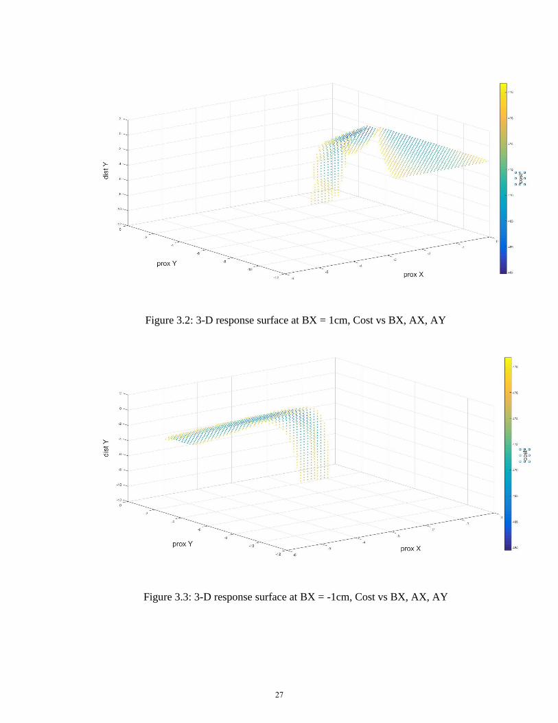
Figure 3.2: 3-D response surface at BX = 1cm, Cost vs BX, AX, AY

Figure 3.3: 3-D response surface at BX = -1cm, Cost vs BX, AX, AY

27

Figure 3.4: 3-D response surface at BX = 2cm, Cost vs BX, AX, AY

As seen in above figures, there is a similar shelf like pattern in all of them. This

shelf is the reason why SPSA is unable to reach to the minimum point which we can be

seen in all the cases. Due to this reason, instead of considering the lowest cost as the actual

solution for the search, any point on that shelf is considered as the solution. This might not

be completely efficient but relatively its better than being not able to find the spring that

satisfies the solution. Moreover, the main priority in here is always given to the design than

obtaining most efficiency for the dominant joint.

This small step back in the algorithm have made it possible to achieve much better

design of the robot making the proximal and distal anchor of the spring stay on the body

of the robot and on the leg of the robot respectively. All these adjustments are explained in

the SPSA section (chapter 2.2) of this document. This about the 4-D search space of this

algorithm. But there are also other two parameters that played a major role in obtaining the

best possible result. One of them is Spring Stiffness. As we have already seen in case of

4-D search that the SPSA algorithm did not perform effectively and using the spring

stiffness or the spring constant as the 5th search parameter will make things even complex.

To avoid this complexity instead of performing a gradient search on the spring stiffness,

28

all the specifications of the springs available in the market that would be helpful for the

robot are logged in and the best suitable for the job are chosen. This gave a total number

of 274 springs. From which only 76 where having the initial length that is required. Then

these 76 combinations are processed through SPSA and the final result is obtained. Based

on these factors the final solution i.e. the anchor points, the spring stiffness and the initial

length of the spring are chosen. These results are shown in next section.

3.2 Walking Results:

After obtaining the results from SPSA algorithm, the particular coordinates for both

the anchor points of the spring are given to the impulsefunction() along with other spring

specifications like the Spring stiffness or spring constant. Depending on all these values

the function gives an analysis of the torques and other factors during one complete stride

period. The whole stride takes 2000 counts.

The various factors analyzed are shown in the figure below

Figure 3.5: Step analysis of the results obtained from SPSA

29

Initial Torque: 526.81, New torque: 379.59, Efficiency: 28%, Initial Length: 0.051m,

Max length: 0.073m, Zero Torque angle: -41.29⁰

To clearly understand each subplot, the individual plots are also shown below

Figure 3.6: Zero torque angle = -41.29⁰

In the above figure is the plot of zero torque angle and the present angle of the motor or

leg. Zero Torque Angle is a point at which the motor doesn’t work against the spring force

rather the spring force is nullified by the placement of the angle of leg itself. This is one

point where we are saving some energy.

Figure 3.7: Extension of the Spring with respect to time

In this figure, the initial spring length is shown in black color and the present spring length

is shown in blue color. This figure gives a clear understanding of the stress applied on the

spring during different phases of the stride.

Figure 3.8: Plots of various torques with respect to time

This figure shows the torque applied by the motor, force applied by the spring and the total

torques ie the summation of the motor torque and the spring force. The blue line is the

original torque applied by the motor, the red line is the force applied by the spring and the

yellow line is the total torque. The direction of these torques also play a major role in this

figure. The torques in the same direction and the new torque less than the original torque

means the spring is helping the system and the if the directions are opposite with same

30

values then the spring is hurting the system. If opposite direction and the blue line is less

than the yellow line, then the spring is helping the system. To make things easy, the

magnitude plot of the above figure is also shown in next figure.

Figure 3.9: Magnitude plot of various torques along with the contact vector

This figure contains the magnitude plots of all the torques. The blue line is the original

torque, the yellow line is the new torque and the black rectangular box kind of line is the

contact of the leg with the ground. If the value is 1, then robot is in Stance phase. If its ‘0’

then the robot’s leg is in Swing phase.

Finally, there is this plot of summation of the overall torque through the whole

stride period and this is shown in the next figure.

Figure 3.10: Integral of all the torques

Blue line is the original torque and the yellow line is the new torque. If the blue line is

greater than the yellow line, that indicates that the spring is helping the system during the

overall stride period.

Flat Terrain:

During all testing and walking the robot only followed one gait which is tripod gait.

The tripod gait follows a constant pattern during all the steps.

31

Figure 3.11: Analysis of different factors, while robot walks 4 steps

Initial torque: 2107.15 N.m, New torque: 1517.86 N.m, initial length of spring: 0.051m,

maximum extended length of spring: 0.073, Zero torque angle: -41.29⁰, efficiency: 28%

Figure 3.12: Subplot of Magnitude of various torques along with the contact vector

during all 4 steps

Figure 3.13: Plot of Magnitude of various torque along with contact vector during single

step.

Here we can see that at 370milliseconds the leg contacts the ground i.e. the robot goes into

stance phase, at this point all the weight of the robot is on the leg. Now, the spring force

comes into play and supports the body weight making the motor exert less torque. This is

32

where most of the energy is saved. If say, the duty cycle of the stride is 75% i.e. the robot

stays in stance phase for 75% of the stride period then all the energy required to generate

torque that can support the body weight during this time is saved. The other time i.e. before

370milliseconds and after 1600 milliseconds the leg stays in the air. During this time, all

the weight of the leg must be supported by the motor and also the spring force acts against

the motor torque. All this together makes the total torque higher than the original torque.

Also, there is one point where spring force doesn’t work against the motor torque even

though the leg is in swing phase. That point is called the Zero torque angle.

Upward Stairs:

Analysis of the results on step up terrain

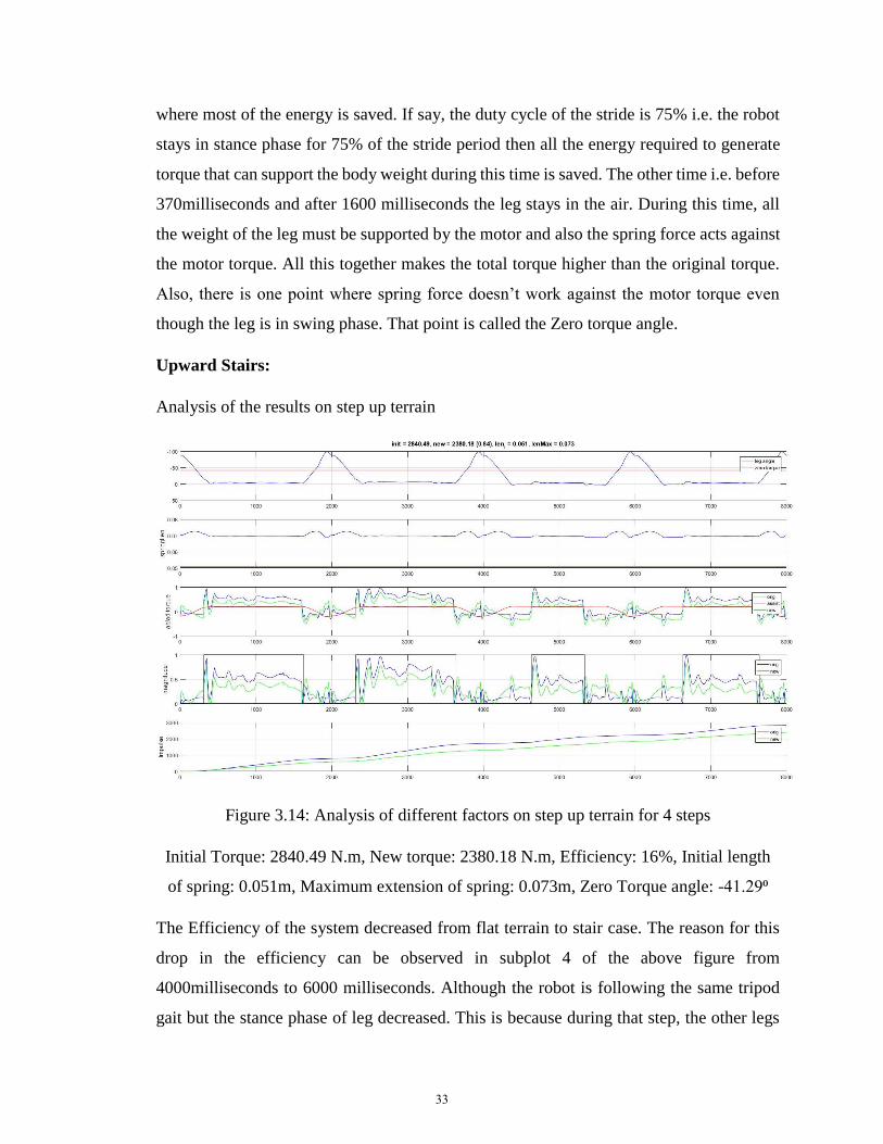
Figure 3.14: Analysis of different factors on step up terrain for 4 steps

Initial Torque: 2840.49 N.m, New torque: 2380.18 N.m, Efficiency: 16%, Initial length

of spring: 0.051m, Maximum extension of spring: 0.073m, Zero Torque angle: -41.29⁰

The Efficiency of the system decreased from flat terrain to stair case. The reason for this

drop in the efficiency can be observed in subplot 4 of the above figure from

4000milliseconds to 6000 milliseconds. Although the robot is following the same tripod

gait but the stance phase of leg decreased. This is because during that step, the other legs

33

of the robot could take over the weight as the found the ground faster due to the stair case

terrain. This made the motor to take all the load of the leg and the spring force. To do so,

the motor must require more torque due to which new torque was 1.05% more than the

original torque.

Random Terrain:

Figure 3.15: Analysis of the various factor on random terrain for 4 steps

Initial Torque: 2555.88 N.m, New Torque: 2266.85 N.m, Efficiency: 11%

As same spring is being used, the initial length of the spring, maximum extension of the

spring and the zero-torque angle will all be same as before. But the difference in efficiency

is due to the randomness of the uneven terrain. During the step from 0 milliseconds to 2000

milliseconds, the stance phase completed way before the normal time, and then

immediately the leg contacted the ground at 1500milliseconds for a small amount of time.

This randomness of the terrain caused the leg to stay in air even though it is in stance phase.

This uncertainty in the time period of the stance phase and the leg contacting the ground

made the motor to take all the load of both leg and spring force.

34

Chapter 4: Future Work:

Number of legs used:

All the data gathered and tested is based on single leg, Leg number #2. The results

obtained from the single leg are used on all the legs which might be better unless the gait

pattern doesn’t change. But if the gait changes, then using same results for all the legs

might not be feasible. Future work could be gathering data for individual leg and finding a

solution for each leg and then testing those solutions.

Different gaits used:

Throughout the work, the only gait used is the Tripod Gait. No other gait is tested.

The results obtained might work even better for other gaits like wave gait. Or the results

obtained by using the data obtained from other gaits might prove to be more efficient.

Future work will be adopting these results on all the legs with multiple gaits.

Multiple Terrain:

In this thesis, the testing is done on single terrain at a time. The data used for

searching the solution was obtained from flat terrain tripod gait walking. The same solution

obtained can be used on multiple terrain like changing from flat terrain to random terrain

with starting the simulation again.

Hardware:

Due to few reasons, the testing was done only on software. In the future, the

obtained spring specifications and the mounting points can be used on a the real hexapod

shown before and the power consumption of the robot can be analyzed.

35

The Big Picture:

Once this system is tested on the hardware with multiple gait patterns, multiple

terrains and based on the results it can be adopted to almost all kind of walking robots. This

system can be made universal. This thesis didn’t talk about the effect on the stability of the

robot. One can also analyze the stability of the robot when this system is used.

36

Chapter 5: References

[1] Firas A. Raheem, Hind Z. Khaleel, ”Static Stability Analysis of Hexagoanl Hexapod

Robot for periodic gaits”, IJCCCE ,Vol. 14, No. 3, 2014

[2] Types of Robot Gait. (n.d.). Retrieved July 27, 2017, from

http://hexapodrobots.weebly.com/types-of-robot-gait.html

[3] Saranli, U.; Buehler, M.; Koditschek, D.E. (2001). "RHex: A Simple and Highly

Mobile Hexapod Robot". The International Journal of Robotics Research. 20 (7): 616.

[4] Aaron M. Hoover, Samuel Burden, Xiao-Yu Fu, S. Shankar Sastry, and R. S. Fearing

(2010).” Bio-inspired design and dynamic maneuverability of a minimally actuated six-

legged robot” International Conference on Biomedical Robotics and Biomechatronics.

[5] LAURON V: A Versatile Six-Legged Walking Robot with Advanced Maneuverability.

IEEE/ASME International Conference on Advanced Intelligent Mechatronics (AIM 2014),

At Besançon, France.

[6] Roennau, Arne; Heppner, Georg; Pfotzer, Lars; Dillmann, Ruediger (July 2013).

"LAURON V: Optimized Leg Configuration for the Design of a Bio-Inspired Walking

Robot".

[7] Passino, K. (2005). Biomimicry for optimization, control, and automation. London:

Springer.

[8] D. E. Goldberg: Genetic Algorithm in Search Optimization, and Machine Learning,

Addiso Wesley, 1989.

[9] Sigeyasu Kawaji and Kazufumi Sawasa: DYTION ROBOT WITH

CHARACTERUSTIC RHYTHM, JAPAN/USA Symposium on Flexible Automation-

Volume 1 ASME 1992

37

[10] Ahmed, M., M.M. Billah, M.R. Khan and S. Farhana, 2009. Walking hexapod robot

in disaster recovery: Developing algorithm for terrain negotiation and navigation. J. World

Acad. Sci. Eng. Technol., 42: 328-333. http://www.waset.com

[11] IEEE and Fraunhofer, 2008. IPA database on service robotics-reconstruction. (n.d.).

Retrieved July 27, 2017, from http://www.ipa.fhg.de/srdatabase/rosy.html

[12] Jun Nishii, Legged insects select the optimal locomotor pattern based on the energetic

cost, Biological Cybernetics, October 2000, Volume 83, Issue 5, pp 435–442

[13] Nishii, J. Biol Cybern (2000) 83: 435. https://doi.org/10.1007/s004220000175,

Springer-Verlag, 0340-1200

[14] Yasuhiro Fukuoka, Kota Fukino, Yasushi Habu and Yoshikazu Mori, Journal:

Bioinspiration & Biomimetics, 2015, Volume 10, Number 4, Page 046017

[15] Taniai, Y., & Nishii, J. (2006). Optimality of the minimum endpoint variance model

based on energy consumption. International Congress Series, 1291, 101-104.

doi:10.1016/j.ics.2006.01.049

[16] Scarfogliero, U., Stefanini, C., & Dario, P. (2009). The use of compliant joints and

elastic energy storage in bio-inspired legged robots. Mechanism and Machine Theory,

44(3), 580-590. doi:10.1016/j.mechmachtheory.2008.08.010

[17] Jiang, W. Y., Liu, A. M., & Howard, D. (2004). Optimization of legged robot

locomotion by control of foot-force distribution. Transactions of the Institute of

Measurement and Control, 26(4), 311-323. doi:10.1191/0142331204tm124oa

[18] Gardner, J. F., Srinivasan, K. and Waldron, K. J. 1990: A solution for the force

distribution problem in redundantly actuated closed kinematic chains. Journal of Dynamic

System, Measurement and Control, Transactions of the ASME 112, 523-526.

[19] Kar, D. C., Issac, K. and Jayarajan, K. 2001: Minimum energy force distribution for a

walking robot. Journal of Robotic Systems 18, 47-54

[20] Kumar, V. R. and Pugh, D. R. 1988: Force distribution in closed kinematics chains.

IEEE Journal of Robotics and Automation 4, 657-663

38

[21] Orin, D. E., & Oh, S. Y. (1981). Control of Force Distribution in Robotic Mechanisms

Containing Closed Kinematic Chains. Journal of Dynamic Systems, Measurement, and

Control, 103(2), 134. doi:10.1115/1.3139653

[22] Santos, P. G., Garcia, E., Ponticelli, R., & Armada, M. (2009). Minimizing Energy

Consumption in Hexapod Robots. Advanced Robotics, 23(6), 681-704.

doi:10.1163/156855309x431677

[23] Huang, Q., Hase, T. and Ono, K. 2007. Optimal trajectory planning method using

inequality state constraint for biped walking robot with upper body mass, Special Issue on

New Trends of Motion and Vibration Control. J. Syst. Des. Dyn. (JSME Dyn. Meas.

Control Div.), 1: 168–179

[24] Nahon, M. A. and Angeles, J. 1992. Minimization of power losses in cooperating

manipulators. J. Dyn. Syst. Meas. Control, 114: 213–219.

[25] Bares, J. E. and Wettergreen, D. S. 1999. Dante II: technical description, results and

lesson learned. Int. J. Robotics Res., 18: 621–649.

[26] Hector Montes, Lisbeth Mena, Roemi Fernández, Manuel Armada. (2017) Energy-

efficiency hexapod walking robot for humanitarian demining. Industrial Robot: An

International Journal 44:4, pages 457-466.

[27] Silva, M. F., & Machado, J. T. (2011). A literature review on the optimization of

legged robots. Journal of Vibration and Control, 18(12), 1753-1767.

doi:10.1177/1077546311403180

[28] Ahmadi M and Buehler M (1999) The ARL monopod II running robot: control and

energetics, in Proceedings of the 1999 IEEE International Conference on Robotics and

Automation, Detroit, MI, May 10–15, pp. 1689–1694

[29] Juárez-Guerrero J, Muñoz-Gutiérrez S and Cuevas WWM (1998) Design of a walking

machine structure using evolutionary strategies. In Proceedings of the 1998 IEEE

International Conference on Systems, Man and Cybernetics, 11-14 October 1998, San

Diego, CA, pp. 1427–1432

39

[30] Lapshin VV (1995) Energy consumption of a walking machine. model estimations

and optimization, in Proceedings of ICAR’95 – Seventh International Conference on

Advanced Robotics, September 1995, Sant Feliu de Guixols, Catalonia, Spain, pp. 420–

425

[31] Neuhaus P and Kazerooni H (2000) Design and control of human assisted walking

robot, in Proceedings of the 2000 IEEE International Conference on Robotics and

Automation, 24-28 April 2000, San Francisco, CA, pp. 563–569

40