1

Income, Value and Returns in Socially Responsible Office Properties

Authors

Gary Pivo1 and Jeffrey D. Fisher2

Forthcoming: Journal of Real Estate Research

May, 2010

Keywords: Corporate Social Responsibility, Sustainability, Energy, Transit, Redevelopment

1 Professor of Urban Planning, University of Arizona, gpivo@u.arizona.edu. 2 Director, Benecki Center for Real Estate Studies and Charles H. and Barbara F. Dunn Professor of Real Estate, Indiana University

2

Abstract Responsible property investing seeks to address social and environmental issues while

achieving acceptable financial returns. It includes strategies such as investing in

properties that are Energy Star labeled, close to transit, and located in redevelopment

areas. We studied the financial performance of these types of properties. With few

exceptions, over the past 10 years they had net operating incomes, market values,

price appreciation and total returns that were higher or the same as conventional

properties, with lower cap rates. We conclude that RPI can be practiced without

diluting returns and can potentially yield higher profits for developers and investors.

1. Background and Objectives

Investors are increasingly interested in socially responsible investing (SRI) (Hill, Ainscough, Shank and Manullang,

2007; Schueth, 2003), or “directing investment funds in ways that combine investors’ financial objectives with their

commitment to social concerns such as social justice, economic development, peace, or a healthy environment”

(Haigh and Hazelton, 2004). A decade ago, Mansley (2000) predicted that property would join the debate on socially

responsible investing because it lies at the frontline of many social and environmental concerns. For example, over

half the world’s greenhouse gas emissions come from operating buildings and the road transport between them

(Metz, Davidson, Bosch, Dave, and Meyer, 2007).

SRI has grown into a global movement (Louche and Lydenberg, 2006). More than 600 institutions have signed the

Principles for Responsible Investment (Principles for Responsible Investment, 2008) and in 2007 SRI investment in

the US encompassed nearly 11 percent of the total investment marketplace (Social Investment Forum, 2008). If just a

tenth of the US SRI investments had been committed to real estate, they would have equaled 87 percent of the total

market capitalization of the US REIT industry (NAREIT, 2009).

In addition to following their personal values, socially responsible investors seek to influence corporate behavior

(Schueth, 2003). According to Rivoli (2003), this can be achieved thru shareholder activism, which can influence

corporate decisions, and thru investment screening, which can alter equity prices, particularly if certain “unrealistic

assumptions” about equity markets having perfect price elasticity are relaxed. Michelson, Wailes, van der Laan and

3

Frost (2004), however, reviewed the literature and found inconclusive evidence that SRI has affected corporate

behavior. But Heinkel, Kraus and Zechner (2001) have demonstrated theoretically that SRI won’t induce reform until

20% of investors participate, and SRI has yet to reach that market share. Haigh and Hazelton (2004) argue that it only

lacks the power so far to create significant corporate change.

When corporations focus on improving their social or environmental performance, they are practicing Corporate

Social Responsibility (CSR). According to Salzmann, Ionescu-Somers and Steger (2005), theorists have argued the

links between corporate financial and social or environmental performance are positive, neutral or negative, while

empirical studies on the subject have been largely inconclusive. A recent review of 167 studies found that CSR

neither harms nor improves returns, concluding that “companies can do good and do well, even if they don’t do well

by doing good” (Margolis and Elfenbein, 2008).

The application of SRI to the property sector is referred to as Responsible Property Investing (RPI) (Mansley, 2000;

McNamara, 2000; Newell and Acheampong, 2002; Boyd, 2005; Lutzkendorf and Lorenz, 2005; Pivo, 2005; Pivo and

McNamara, 2005; Pivo, 2007; Rapson, Shiers, and Keeping, 2007; UNEP FI, 2007; Newell, 2008). The Journal of

Property Investment and Finance recently published a special issue on the topic in which the editor argues that

property has a role to play in every category of corporate responsibility including environment, workplace, diversity,

community, and corporate governance (Roberts, 2009).

RPI is broadly concerned with investment and development decisions that are responsive to the social, environmental

and economic concerns of all affected stakeholders. Previously, professional real estate ethics has focused mostly on

decision-making in the best interest of clients, unimpaired by personal self-interest (Levy and Terflinger, 1988). RPI,

however, expands the range of parties whose interests’ decision makers should consider and seeks out investment

and development strategies that improve the well-being of both immediate professional clients as well as other

groups, such as neighbors, construction workers, maintenance personnel, building users, other species and future

generations.

Unfortunately, what little we know about the ethical standards among real estate professionals paints a less than

flattering picture. Izzo (2000), using standardized measures of cognitive moral development, found that only 25

percent of Realtors were “principled”, or of the view that one should act according to universal ideas of justice and

4

promote the general welfare. The rest exhibited either “conventional” moral reasoning, meaning they follow the law

and do what’s expected of them, or “preconventional” reasoning, meaning they follow rules only when it’s in their

immediate self-interest. Meanwhile, Velthouse and Kandogan (2006) found that the “aggregate ethics” rating for

managers in the finance, insurance and real estate (FIRE) sector was the lowest of the nine sectors studied.

However, contrary to these findings, more than 85 percent of US property investment executives would increase their

allocation to RPI if it met their risk and return criteria (Pivo, 2008a). They are concerned, however, about its potential

financial performance. How ethically screened investments perform in comparison to conventional ones is a

contentious issue (Michelson, Wailes, van der Laan and Frost, 2004; Bauer, Koedijk and Otten, 2005) and findings

are mixed on whether investors will sacrifice financial returns for social responsibility (Rosen, Sandler and Shani,

2005; Nilsson 2007; Vyvyan, Ng and Brimble, 2007; Williams, 2007). But if RPI does harm values or returns, it will

undoubtedly face resistance. In this study, therefore, we examined the relationship between RPI, market value, and

investment returns by comparing the financial performance of RPI and non-RPI office properties throughout the US

from 1999-2008.

To complete the study we had to define and identify RPI properties. Fortunately, we could rely on a recent

international survey of stakeholders that ranked RPI criteria. It concluded that the most important goals should be “the

creation of less automobile-dependent and more energy-efficient cities where worker well-being and urban

revitalization are priorities” (Pivo, 2008b). Consequently, we focused on 3 specific types of office properties: those

close to transit stations, those with the Energy Star label, and those in urban revitalization areas.

2. Research Hypotheses

RPI features that affect occupancy, rent or operating expenses should affect net operating income (NOI). If transit

improves accessibility (Geurs and van Wee, 2004), then properties near it should have higher rents and occupancy.3

If energy efficiency lowers power bills (Kats and Perlman, 2006), then Energy Star properties should have lower

3 Some cities grant tax abatements to developers who build near transit. Most of the properties near transit in this study, however, were not built as part of formal transit-oriented development projects and ineligible for incentives.

5

expenses.4 And if business in redevelopment areas receives government incentives

5 (Lynch and Zax, 2008), then

properties there could have higher rents and occupancy. So, our first hypothesis was that properties near transit,

energy efficient properties and properties in areas targeted for redevelopment have had a higher average NOI.

Since property values are a function of income flows and capitalization rates, RPI features that affect them should

affect values. If we expect RPI properties to have higher NOI, we should also expect higher valuations. And if they are

viewed as safer investments, their values should be even higher, assuming capitalization rates are inversely related to

risk. Uncertainties about energy costs and regulations may have caused investors to view energy efficient properties

and properties near transit as safer investments. But weak demand in regeneration areas may have caused them to

be seen as riskier. Alternatively, investors could have accepted lower cap rates for properties in revitalization areas if

they saw greater potential for income growth by filling vacant spaces (Sivitanides, 1998). So, our second hypothesis

was that properties near transit and energy efficient properties have had lower cap rates and higher values while the

results in redevelopment areas have been more ambiguous.

Total investment return is composed of appreciation and income returns. Superior appreciation can occur if incomes

grow faster than previously anticipated, or if faster income growth or slower depreciation is expected in the future.

Income return is the ratio of income to the property value at a given point in time. It is analogous to the capitalization

rate. If an RPI property is expected to produce higher future incomes, it could produce higher appreciation and

therefore be purchased at lower income returns in order to achieve the same total returns. That is, properties with

more expected growth in income and value will tend to have lower cap rates.

For Energy Star properties and properties near transit, we thought that trends over the past several years may have

produced positive effects on appreciation and downward pressure on income returns, resulting in a neutral effect on

total returns. Trends in gas and electricity prices (see Exhibit 1) illustrates why this may have been so. It shows the

increase in gasoline and electricity prices for the three most recent 5 year periods. In the last two, prices grew much

faster than before. If we assume investors had been projecting future costs based on past trends, they would have

4 Energy efficient properties may also benefit from incentives offered by government and utilities including tax deductions, utility rebates, low interest loans, and expedited permitting. Utility rebates can directly affect net operating expenses by lowering utility expenditures. 5 Government incentives can include property tax abatements, sale tax exemptions, income tax deductions, employment credits, no tax on capital gains, increased deductions on equipment, accelerated real property depreciation, and more.

6

projected slower increases than actually occurred. A discontinuity in prices could have produced an unexpected shift

in demand toward energy efficient and transit-oriented properties, causing their incomes to grow faster than

anticipated and producing superior appreciation. Meanwhile, growing concern about the risks of owning energy

inefficient and auto dependent properties may have produced downward pressure on cap rates for Energy Star and

transit-oriented properties, lowering their income returns. The net result on total returns, however, may well have been

neutral. So, our third hypothesis was that energy efficient and transit-oriented properties have generated a higher

appreciation return and a lower income return (cap rate) than otherwise similar properties.

Exhibit 1 | Trends in Gas and Electricity Prices (mean annual percent change)

1993-1998 1998-2003 2003-2008

Gasoline, regular grade, nominal price -.08 9.5 14.6

Electricity, end use commercial sector, nominal price -1.3 1.6 4.4

Note: Data from the US Department of Energy, Energy Information Administration.

3. Literature Review

The only studies to directly examine the empirical effects of redevelopment programs on non-residential property

come from the UK. Erickson and Syms (1986) found that properties in enterprise zones commanded higher rents.

Twenty years later McGreal, Webb, Adair and Berry (2006) found that returns in urban renewal districts matched

returns for conventional properties. Both studies support our hypotheses that properties in redevelopment areas have

had higher incomes and similar returns compared to properties outside redevelopment areas. Malizia (2003),

however, using qualitative methods, found that participants in redevelopment projects viewed them as riskier

investments and that appraisers apply higher cap rates to reflect that risk.

Four studies have found rent and price premiums in energy efficient office buildings (Eichholtz, Kok, and Quigley,

2009; Fuerst and McAllister, 2008; Miller, Spivey and Florance, 2008; Wiley, Benefield and Johnson, 2008). Miller,

7

Spivey and Florance (2008) also found lower cap rates. Studies on housing produced similar results: efficiency was

capitalized into value (Corgel, Goebel and Wade, 1982; Longstreth, 1986; Laquatra, 1986; Dinan and Miranowski,

1989). These studies support our expectation that energy efficiency benefits incomes and values. We found no prior

work on energy efficiency and investment returns.

Cervero, Ferrell and Murphy (2002) summarized the prior research on transit. They concluded that “numerous studies

have demonstrated that being near rail stops raises property values.” Benjamin and Sirmans (1996), working on

Washington D.C. apartment rents, also found a positive effect for proximity to transit. Some studies, however, have

reached contrary conclusions (Bollinger, Ihlanfeldt and Bowes, 1998; Gatzlaff and Smith, 1993; Nelson, 1992). Since

Cervero, Ferrell and Murphy (2002), three more papers have been published. Ryan (2005) found that access to light

rail transit in San Diego was insignificant for office and industrial rents while Duncan (2008) found it was positive for

single family home and condominium values. Meanwhile, Hess and Almeida (2007) found that light rail stations in

Buffalo increased single family home values while Portnov, Genkin and Barzila (2009) found that urban rail lines had

a negative effect on multi-story apartment sale prices within 100 meters of the tracks and then a positive effect

beyond. Most of this literature focuses on rents and valuations. Only one study examined appreciation. Clower and

Weinstein (2002) found that office property values near Dallas light rail stations increased at more than twice the rate

of other properties from 1997 to 2001.

Overall, where prior quantitative studies have addressed our concerns, they have mostly supported our hypotheses.

They show that properties in redevelopment areas commanded higher rents but did not outperform on returns, that

energy efficient properties had higher rents and values, and that in several instances properties near transit were

more valuable and appreciated faster than in other locations. Our paper tests the validity of these findings and thereby

strengthens our general understanding. But we also break new ground. We report the first findings on office incomes,

values and returns in US areas receiving economic development incentives. We also offer the first look at investment

returns for energy efficient offices, and while ours is not the first study to look at office returns near transit, it is just the

second to do so and the first to do it on a national scale. Indeed, a strength of this project was its use of national data.

Only the papers cited on energy efficient offices used national data. Most studies looked at one or a few metropolitan

areas, restricting their ability to make national generalizations which are useful to developers and investors operating

on a national scale.

8

4. Methods and Data

We used this model to test our hypotheses

Pij = f (Rj, Ni, Eij, Ri, Ai, Qi, Gij, ui) (1)

Where, Pij = a vector of variables describing the performance of the ith property in year j, Rj = a vector of variables

describing the RPI features of the ith property, Nj = the national office market conditions in year j, Eij = a vector of

variables describing the economy of the region of the ith property in year j, Ri = the regional location of the ith

property, Ai = a vector of variables describing the accessibility conditions for the ith property, Qi = a vector of variables

describing the quality of the ith property, Gi = a vector of variables describing the cost of government services for the

ith property in year j, and ui = a stochastic term. We considered whether we should expect apriori any interaction

between the RPI variables (i.e. whether their affect on performance should depend on whether a property had any of

the other RPI features studied) and concluded there would not be. We also tried different interactions and did not find

that they added to the explanatory power of the model. Consequently, to avoid reducing parsimony and increasing the

difficulty of interpretation we did not use interaction variables in the model.

Quarterly data for 1999-2008 were compiled for office properties from data maintained by the National Council of Real

Estate Investment Fiduciaries (NCREIF). NCREIF is a source of real estate performance information based on

property-level data submitted by its data contributing members, which include institutional investors and investment

managers. Properties are added to or removed from the database as members acquire or sell holdings. Our sample

consisted of all the office properties in the NCREIF database that had complete addresses and could be geocoded.

That came to 1,199 properties with a total market value of about $98 billion. The addresses were needed in order to

obtain information from other data sources (discussed further below). Since properties were added to and deleted

from the dataset as they are bought and sold, the number of properties in the sample varied somewhat over time. The

number of observations in any particular regression ranged from approximately 6,000 to 7,500 observations,

depending on the specific variables used because of missing data for some properties.

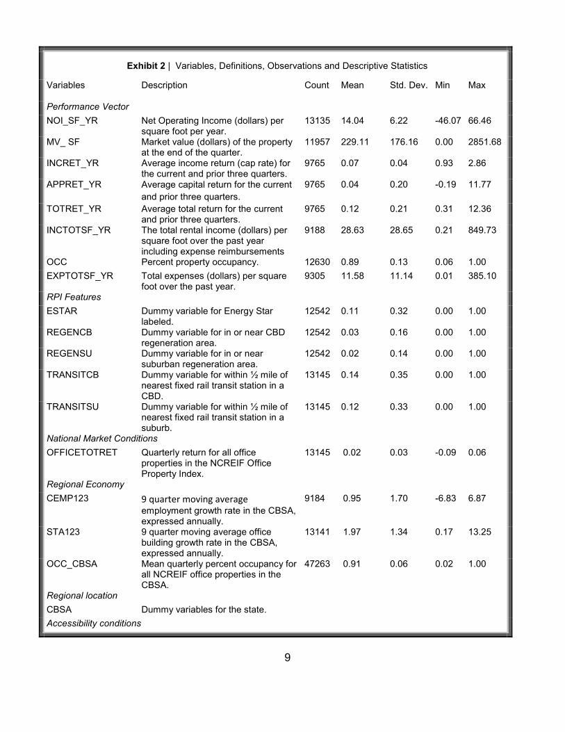
Exhibit 2 summarizes the variables used in the study and gives their descriptive statistics.

9

Exhibit 2 | Variables, Definitions, Observations and Descriptive Statistics

Variables Description Count Mean Std. Dev. Min Max

Performance Vector

NOI_SF_YR Net Operating Income (dollars) per square foot per year.

13135 14.04 6.22 -46.07 66.46

MV_ SF Market value (dollars) of the property at the end of the quarter.

11957 229.11 176.16 0.00 2851.68

INCRET_YR Average income return (cap rate) for the current and prior three quarters.

9765 0.07 0.04 0.93 2.86

APPRET_YR Average capital return for the current

and prior three quarters.

9765 0.04 0.20 -0.19 11.77

TOTRET_YR Average total return for the current and prior three quarters.

9765 0.12 0.21 0.31 12.36

INCTOTSF_YR The total rental income (dollars) per square foot over the past year including expense reimbursements

9188 28.63 28.65 0.21 849.73

OCC Percent property occupancy. 12630 0.89 0.13 0.06 1.00

EXPTOTSF_YR Total expenses (dollars) per square foot over the past year.

9305 11.58 11.14 0.01 385.10

RPI Features

ESTAR Dummy variable for Energy Star labeled.

12542 0.11 0.32 0.00 1.00

REGENCB Dummy variable for in or near CBD regeneration area.

12542 0.03 0.16 0.00 1.00

REGENSU Dummy variable for in or near suburban regeneration area.

12542 0.02 0.14 0.00 1.00

TRANSITCB Dummy variable for within ½ mile of nearest fixed rail transit station in a CBD.

13145 0.14 0.35 0.00 1.00

TRANSITSU Dummy variable for within ½ mile of nearest fixed rail transit station in a suburb.

13145 0.12 0.33 0.00 1.00

National Market Conditions

OFFICETOTRET Quarterly return for all office properties in the NCREIF Office Property Index.

13145 0.02 0.03 -0.09 0.06

Regional Economy

CEMP123 9 quarter moving average employment growth rate in the CBSA, expressed annually.

9184 0.95 1.70 -6.83 6.87

STA123 9 quarter moving average office building growth rate in the CBSA, expressed annually.

13141 1.97 1.34 0.17 13.25

OCC_CBSA Mean quarterly percent occupancy for all NCREIF office properties in the CBSA.

47263 0.91 0.06 0.02 1.00

Regional location

CBSA Dummy variables for the state.

Accessibility conditions

10

TRAVHOMEWORK Mean travel time in minutes from home to work by all modes for all workers in the census tract.

12936 24.20 5.50 4.00 46.00

BLK_GP_POPDEN 2007 census block group population density.

13145 6518.62 12023.82 0.00 110566.7

STYPE Dummy variable for in CBD. 13145 0.19 0.40 0.00 1.00

MSADENS Population density of the CBSA in

persons per acre.

9184 6.82 0.83 4.61 8.81

Property quality

SQFT Square feet of the building. 13145 271168.5 364378.4 8022 2.26E+07

FLOORS Number of floors. 13145 7.52 9.94 0.00 76.00

FLOORS2 Number of floors squared.

AGE Age of the property in years. 11899 19.91 17.30 0.00 123.00

Cost of government Services

EFFPROPTAX Effective property tax rate in the quarter for the CBSA.

12586 0.02 0.01 0.00 0.23

4.1 Financial Performance Variables

To examine the impact of RPI on values, NCREIF provided appraised values for the properties that had not sold and

transaction prices for properties that had sold -- the same appraisals and transaction prices used to calculate the

quarterly NCREIF Property Index. Many of the other models we examined such as NOI, expenses, occupancy, etc.

were based on actual accounting data gathered by NCRIEF from the building owners. Those data did not come from

appraisers and were not survey data.

Many studies have shown that appraised values tend to lag transaction prices by a few quarters in appraisal-based

indices (Geltner and Ling, 2006). One reason for this is the nature of the appraisal process which relies on historical

data such as comparable sales. Another reason is that not all properties are actually revalued every quarter. Some

may only be revalued two or three times a year. However, virtually all of the properties in the NCREIF set are

revalued at least once a year. Since the purpose of this study was to examine cross-sectional differences in property

values as a result of different RPI characteristics, a delay of a quarter or two in updating the appraised value of a

particular property would not significantly impact the relative cross-sectional differences in properties. Said differently,

since properties with and without a particular RPI characteristic have the same appraisal lag, the cross-sectional

comparisons are on an apples-to-apples basis.

11

It should be noted that bias associated with appraisal smoothing at the individual property level is different from that at

the index level. There are "unsmoothing techniques" that can be applied at the index level to account for the fact that

not all properties are revalued every quarter (Fisher and Geltner, 2000). But this is not appropriate for individual

properties. The problem caused by individual properties not being revalued every quarter is that in those quarters the

property is not revalued, there will be no change in value and the return is biased toward zero. Furthermore, when

there is a revaluation, the return will reflect all the change in value since the last appraisal. Since properties in the

index are revalued at least once a year, we used a four quarter moving average of returns as our dependent variable.

This allowed us to better capture the trend in returns than using single quarter returns. Each observation reflected

how values had changed on average over the past four quarters rather than having some quarters with no change in

value and others with too high (or too negative) a change in value that reflected more than one quarter. Because

quarterly returns tended to be correlated over time, we used a panel regression with clustering at both the property

and year level as a robustness test to be sure the independent variables of interest were still significant and we found

they were.

4.2 RPI Variables

Energy Star labeling was used to define whether or not a property was energy efficient. Labeling information was

collected from the US EPA Energy Star Program. To be labeled, a building must be in the top quartile of energy

efficiency when compared to peers (i.e. office buildings with similar operational characteristics including size, weather

conditions, number of occupants, number of computers, and hours of operation per week).

Data on the latitude and longitude of all US fixed rail transit stations were obtained from the U.S. Bureau of

Transportation Statistics (BTS), National Transportation Atlas Database. This included stations for commuter trains,

heavy rail, light rail, and monorail. Supplemental data from Google Earth were used for the New York area. The

straight line distance from each property to the nearest rail transit station was measured using GIS software.

Properties that were ½ mile or less from a transit station were categorized as transit-oriented properties.6

6 We also used a quarter mile to define properties near transit but found the half mile distance to be a better predictor in the

models.

12

Data used to define urban regeneration properties came from the US Department of Housing and Urban Development

(HUD). They were defined as those located in or near an Empowerment Zone, Renewal Community, or Enterprise

Community as defined by HUD’s online RC/EZ/EC Address Locator.

4.3 Controls Variables

As indicated by Equation (1), we used several controls in order to isolate the effects of the RPI features on property

performance. National market conditions each year were controlled with the NCREIF office market index. Regional

economic conditions were controlled with the yearly growth rate of office buildings in the region as a measure of local

supply, the yearly regional employment growth rate as a measure of local demand and office occupancy rates as a

measure of supply/demand balance. Since the NCREIF office market index for each year controlled for changes in

the national market over time, the regional supply, demand and occupancy variables only captured differences

between CBSAs. CBSA dummy variables controlled for static regional conditions not otherwise controlled.

We used four variables to control for intraregional location and accessibility conditions. Regional accessibility at each

property location was controlled using the mean travel time to work from homes in the census tract and the population

density in the census block group. We might have used traditional gravity-based and distance to CBD measures

(Song 1996, Geurs and Wee, 2004) but that was infeasible given the large number of properties and regions in our

study. Levinson (1998) demonstrates that journey to work time is a good proxy for gravity-based accessibility

measures and Heikkila and Peiser (1992) show that accessibility co-varies with urban density at the block group level.

A dummy for whether or not properties were in a CBD provided additional control on access to the CBD. Metropolitan

level population density was used as a proxy for regional congestion and mobility. We found that population density at

the metro scale is correlated with direct congestion measures published by the Texas Transportation Institute (r = .45

- .55) but their measures were unavailable for all regions in our study. Note that this density measure is for the entire

metropolitan area and does not measure density in the vicinity of each property. It should not be confused with our

measures for accessibility at the property scale, including block group population density.

Size and age were used to control for quality. Building class, another measure of building quality, has been found to

be related to rent and values (Glascock, Jahanian and Sirmans, 1990; Eichholtz, Kok, and Quigley, 2009) but it was

unavailable for this study. However, “classifications of offices are far from precise” and typically rely on vintage and

location to make class distinctions (Archer and Smith 2003), which we control for using age and the location variables.

13

We also control for stories (FLOORS and FLOORS2), which is most likely related to the “market presence” dimension

of building class. We do not directly control for finishes and building systems, which are additional elements of class,

but they probably co-vary with the variables we do control. Evidence that age and stories can substitute for class can

be found in Eichholtz, Kok, and Quigley (2009) which presents models estimating office rent and values. In their

models, the coefficients for Class A and B dummies are reduced by about half when variables for age and stories are

introduced. Nevertheless, Dermisi and McDonald (2010) have found that for Chicago office buildings, Class A

increased selling price per square foot compared to Class B, holding numerous other building features constant. It

would seem, then, that we could improve our findings by introducing building class as a control variable.

Effective tax rate paid by each property was computed from NCREIF tax expenditure and property value data. The

mean rate at the CBSA level was used to control for the cost of local government services. We did not control for any

government or utility incentives provided to RPI properties. As discussed in footnotes 1-3, some RPI properties,

depending on their location, can benefit from economic incentives that may increase their income and value. If these

were controlled in the analysis, any positive effects of RPI features would likely be diminished. And in the case of the

redevelopment properties studied, which by definition are eligible for federal incentives, controls for financial

incentives would probably eliminate all significant effects. Consequently, changes to pertinent incentive programs

would likely alter the relationships found in this study.

For two of the RPI characteristics (near transit and in or near urban regeneration zones), we used separate dummy

variables to indicate whether a property had these characteristics and was in a CBD or suburb. For example,

TRANSITCB was 1 if the property was near transit in the CBD and 0 otherwise (meaning that it was not near transit in

either a CBD or a suburb or near transit in a suburb). Similarly TRANSITSU was 1 if it was near transit in a suburb

and 0 otherwise. There is also a dummy variable, STYPE, indicating whether a property was in a CBD or suburb,

regardless of whether it had an RPI characteristic or not. If STYPE was 1, the property was in a CBD and if it was 0, it

was in a suburb. With this structure of dummy variables, what the STYPE variable captured was the difference that

being in a CBD versus a suburb had on Energy Star and non-RPI properties because the relative impact of the transit

and urban regeneration RPI variables caused by being in a CBD or suburb was already captured in the dummy

variables already included for these characteristics. For example, if the only RPI variables in a regression were

TRANSITCB and TRANSITSU, with the market value as the dependent variable, then STYPE captured the difference

14

in market value for the non-transit property in a CBD compared to the non-transit property in the suburb. Meanwhile,

the TRANSITCB variable captured the marginal impact on market value of being near transit in a CBD relative to not

being near transit in a CBD. Likewise, the TRANSITSU variable captured the marginal impact on market value of

being near transit in a suburb versus not being near transit in a suburb. This setup for the dummy variables allowed

us to capture the impact of each RPI variable in the CBD relative to those properties that did not have this RPI

characteristic in a CBD and similarly in a suburb. As we will see, the impact of some of the RPI characteristics is

different in a CBD than in a suburb. Although STYPE could be omitted and a dummy variable added to indicate

whether a property did not have one of the RPI characteristics in, say, a CBD (with not having the RPI characteristic

in the suburb being the omitted dummy variable), this would cause dependency problems among the independent

variables when there is more than one RPI characteristic because the dummies for each set of RPI variables define

whether the property is in a CBD or not.

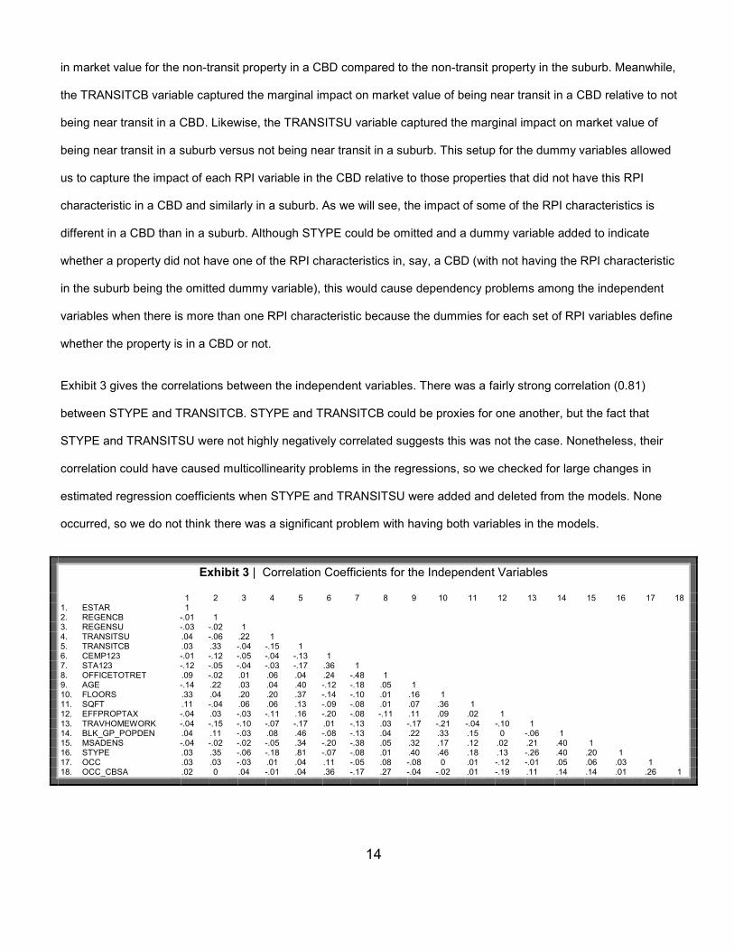
Exhibit 3 gives the correlations between the independent variables. There was a fairly strong correlation (0.81)

between STYPE and TRANSITCB. STYPE and TRANSITCB could be proxies for one another, but the fact that

STYPE and TRANSITSU were not highly negatively correlated suggests this was not the case. Nonetheless, their

correlation could have caused multicollinearity problems in the regressions, so we checked for large changes in

estimated regression coefficients when STYPE and TRANSITSU were added and deleted from the models. None

occurred, so we do not think there was a significant problem with having both variables in the models.

Exhibit 3 | Correlation Coefficients for the Independent Variables

1 2 3 4 5 6 7 8 9 10 11 12 13 14 15 16 17 18 1. ESTAR 1 2. REGENCB -.01 1 3. REGENSU -.03 -.02 1 4. TRANSITSU .04 -.06 .22 1 5. TRANSITCB .03 .33 -.04 -.15 1 6. CEMP123 -.01 -.12 -.05 -.04 -.13 1 7. STA123 -.12 -.05 -.04 -.03 -.17 .36 1 8. OFFICETOTRET .09 -.02 .01 .06 .04 .24 -.48 1 9. AGE -.14 .22 .03 .04 .40 -.12 -.18 .05 1 10. FLOORS .33 .04 .20 .20 .37 -.14 -.10 .01 .16 1 11. SQFT .11 -.04 .06 .06 .13 -.09 -.08 .01 .07 .36 1 12. EFFPROPTAX -.04 .03 -.03 -.11 .16 -.20 -.08 -.11 .11 .09 .02 1 13. TRAVHOMEWORK -.04 -.15 -.10 -.07 -.17 .01 -.13 .03 -.17 -.21 -.04 -.10 1 14. BLK_GP_POPDEN .04 .11 -.03 .08 .46 -.08 -.13 .04 .22 .33 .15 0 -.06 1 15. MSADENS -.04 -.02 -.02 -.05 .34 -.20 -.38 .05 .32 .17 .12 .02 .21 .40 1 16. STYPE .03 .35 -.06 -.18 .81 -.07 -.08 .01 .40 .46 .18 .13 -.26 .40 .20 1 17. OCC .03 .03 -.03 .01 .04 .11 -.05 .08 -.08 0 .01 -.12 -.01 .05 .06 .03 1 18. OCC_CBSA .02 0 .04 -.01 .04 .36 -.17 .27 -.04 -.02 .01 -.19 .11 .14 .14 .01 .26 1

15

5. Results and Discussion

We now turn to the regression analyses. In most cases the controls were significant and had the expected signs. R-

squares varied depending on the regression. Our focus, however, was on the significance of the RPI variables and

not the predictive power of the models.

5.1 Income and Market Value

In the following two models we used log transformed dependent variables to reduce skewness and facilitate

interpretability of the coefficients. The models show that over the past 10 years, RPI properties had NOIs and market

values per square foot that were equal to or higher than conventional office investments. In no case did the RPI

features harm incomes or values.

5.1.1 Net Operating Income (NOI) per Square Foot

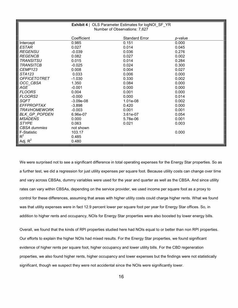
As indicated by the coefficients in Exhibit 4, the NOI per square foot for Energy Star properties was 2.7 percent higher

than for non Energy Star properties and 8.2 percent higher for CBD regeneration properties compared to other CBD

offices. Suburban regeneration and transit properties had NOIs that were similar to non-RPI properties.

As already discussed, higher NOI can be from higher rents, higher occupancy or lower expenses. To determine which

of these might be driving the higher NOIs, we examined whether ESTAR and REGENCB could explain rents,

occupancy and expenses by using them as dependent variables in separate regression models. We found that

Energy Star properties had 5.2 percent higher rents than other properties and CBD regeneration properties had 4.8%

higher rents than other CBD offices, although the later was statistically insignificant. This Energy Star rent premium is

less than the 7.3 to 11.6 percent premium found by others (Wiley, Benefield and Johnson, 2008; Fuerst and

McAllister 2008; Eichholtz, Kok, and Quigley, 2008). We found that occupancy was 1.3 percent higher for Energy Star

properties and 0.2 percent higher for the CBD regeneration properties, but the later was again insignificant. Both

properties had lower total operating expenses but neither result was statistically significant.

16

Exhibit 4 | OLS Parameter Estimates for logNOI_SF_YR Number of Observations: 7,627

Coefficient Standard Error p-value Intercept 0.985 0.151 0.000 ESTAR 0.027 0.014 0.045 REGENSU -0.039 0.036 0.276 REGENCB 0.082 0.027 0.002 TRANSITSU 0.015 0.014 0.284 TRANSITCB -0.025 0.024 0.300 CEMP123 0.008 0.004 0.027 STA123 0.033 0.006 0.000 OFFICETOTRET -1.030 0.330 0.002 OCC_CBSA 1.350 0.084 0.000 AGE -0.001 0.000 0.000 FLOORS 0.004 0.001 0.000 FLOORS2 -0.000 0.000 0.014 SQFT -3.09e-08 1.01e-08 0.002 EFFPROPTAX -3.898 0.420 0.000 TRAVHOMEWORK -0.003 0.001 0.001 BLK_GP_POPDEN 6.96e-07 3.61e-07 0.054 MSADENS 0.000 5.78e-06 0.001 STYPE 0.063 0.021 0.003 CBSA dummies not shown F-Statistic 103.17 0.000 R2 0.485

Adj. R2 0.480

We were surprised not to see a significant difference in total operating expenses for the Energy Star properties. So as

a further test, we did a regression for just utility expenses per square foot. Because utility costs can change over time

and vary across CBSAs, dummy variables were used for the year and quarter as well as the CBSA. And since utility

rates can vary within CBSAs, depending on the service provider, we used income per square foot as a proxy to

control for these differences, assuming that areas with higher utility costs could charge higher rents. What we found

was that utility expenses were in fact 12.9 percent lower per square foot per year for Energy Star offices. So, in

addition to higher rents and occupancy, NOIs for Energy Star properties were also boosted by lower energy bills.

Overall, we found that the kinds of RPI properties studied here had NOIs equal to or better than non RPI properties.

Our efforts to explain the higher NOIs had mixed results. For the Energy Star properties, we found significant

evidence of higher rents per square foot, higher occupancy and lower utility bills. For the CBD regeneration

properties, we also found higher rents, higher occupancy and lower expenses but the findings were not statistically

significant, though we suspect they were not accidental since the NOIs were significantly lower.

17

5.1.2 Market Value per Square Foot

Higher NOIs should produce higher property values, assuming the same level of risk, and that is in fact what we

found. This suggests that the effects of RPI features on NOI were being capitalized into market values. We also found

cases of higher values without higher NOI, where higher values were probably being driven by lower capitalization

rates.

As indicated by the coefficients in Exhibit 5, Energy Star properties were worth 8.5 percent more per square foot than

other properties.7 This compares to value premiums of 5.8% to 19.1% reported in other recent studies (Miller, Spivey

and Florance, 2008; Fuerst and McAllister, 2008; Wiley, Benefield and Johnson, 2008; Eichholtz, Kok, and Quigley,

2008). Our results fall into the lower range of these other findings, but the other studies model exchange prices rather

than appraised values and appraised values can lag behind exchange values, as already noted. And if the value of

Energy Star properties grew most quickly in the later part of the study period, then a lag of a few quarters could be

significant. Other possible explanations for our lower premium could be that the other studies used different samples

and fewer controls. Nonetheless, our results are consistent with the conclusion of every study to date: there has been

a significant value premium associated with Energy Star properties.

Market values for regeneration properties were no different from other properties in the suburbs and 6.7 percent

higher in the CBDs. Properties near transit were 10.6 percent more valuable per square foot in the suburbs and 9.1

percent more valuable in the CBDs. These are also notable results indicating again that the RPI features in this study

appear to range from neutral to quite positive for property values.

The RPI properties that had higher NOIs (Energy Star and CBD Regeneration) also had higher market values, as

expected; however for Energy Star properties the value premium was more than triple the NOI premium. In addition,

both types of transit properties had higher values without higher NOIs. But value is a function of both NOI and

capitalization rate, and as we show in the next section, the value premiums that cannot be explained by higher NOIs

can be explained by lower cap rates.

7 We also separated Energy Star properties into CBD and suburban subgroups, with similar results.

18

Exhibit 5 | OLS Parameter Estimates for logMV_SF Number of Observations: 7,647

Coefficient Standard Error p-value Intercept 3.952 0.153 0.000 ESTAR 0.085 0.014 0.000 REGENSU -0.033 0.037 0.375 REGENCB 0.067 0.027 0.014 TRANSITSU 0.106 0.014 0.000 TRANSITCB 0.091 0.024 0.000 CEMP123 0.024 0.004 0.000 STA123 0.002 0.006 0.773 OFFICETOTRET 6.608 0.334 0.000 OCC_CBSA 0.760 0.086 0.000 AGE -0.006 0.000 0.000 FLOORS 0.011 0.001 0.000 FLOORS2 -0.000 0.000 0.010 SQFT -1.76e-07 1.03e-08 0.000 EFFPROPTAX -8.636 0.427 0.000 TRAVHOMEWORK -0.018 0.001 0.000 BLK_GP_POPDEN 1.32e-06 3.66e-07 0.000 MSADENS 0.000 5.86e-06 0.000 STYPE 0.077 0.022 0.000 CBSA dummies not shown F-Statistic 162.84 0.000 R2 0.597

Adj. R2 0.594

5.2 Investment Returns

The next three models examine the impact of RPI features on investment returns. The log of 1 + return was used as

the dependent variable because returns could be negative. Many of the controls were dropped because they were not

significantly related to returns. Overall, we found that RPI features did not affect total returns. However, when

disaggregated into income and appreciation returns, we found lower income returns for most of the RPI property

types, suggesting that they were favored in the capital asset market and that owners were willing to buy these

properties at a lower capitalization rate.

5.2.1 Income Returns

As indicated in Exhibit 6, Energy Star lowered income returns by 0.5 percent (rounded from 52 basis points). There

are three possible explanations for these results. First, owners might have been anticipating higher income growth,

faster appreciation or slower depreciation. Second, owners might have been anticipating slower growth in operating

expenses. And third, owners might have viewed these properties as less exposed to risks from energy shocks and

19

regulations. It is remarkable that Miller, Spivey and Florance (2004), working with a different sample, found that taken

together, LEED certified and Energy Star labeled buildings had cap rates that were 55 basis points lower than other

properties, which is nearly identical to our results.

Exhibit 6 | OLS Parameter Estimates for logINCRET_YR Number of Observations: 6,039

Coefficient Standard Error p-value Intercept 0.972 0.162 0.000 ESTAR -0.005 0.001 0.000 REGENSU -0.003 0.003 0.390 REGENCB 0.005 0.003 0.091 TRANSITSU -0.004 0.001 0.001 TRANSITCB -0.015 0.002 0.000 CEMP123 -0.003 0.000 0.000 STA123 0.002 0.001 0.028 OFFICETOTRET -0.281 0.045 0.000 OCCUPANCY 0.099 0.003 0.000 OCC_CBSA -0.017 0.010 0.101 MSADENS -0.000 0.000 0.000 STYPE 0.004 0.002 0.082 CBSA dummies not shown F-Statistic 33.72 0.000 R2 0.301

Adj. R2 0.292

We also found that proximity to transit reduced income returns by 0.4 percent in the suburbs and 1.5 percent in the

CBDs. In this case concerns about gas prices, carbon taxes, traffic congestion, and accessibility issues, along with

forecasted growth in demand toward transit properties (Center for Transit Oriented Development, 2004), may have

been shaping what investors were willing to pay for less auto-dependent properties.

The lower capitalization rates for certain types of RPI properties help explain the higher market values which could not

be fully explained by higher NOIs. In particular, while a 8.5 percent higher market value per square foot in Energy Star

properties could not be explained by just 2.7 percent higher NOI, it could be explained by a combination of higher NOI

and lower cap rates.8 We also found that transit properties had higher market values without higher NOIs. Here again,

8 Using the mean NOI per square foot and mean cap rate (i.e. income return) from Exhibit 2, we computed a mean market value

per square foot of about $201. When we then adjusted NOI upward by 2.7% and the cap rate downward by 0.05%, we

computed a mean market value of $222 per square foot, which equals a market value premium of about 10%.

20

the gap could be explained by lower cap rates. The reverse was also true: when we found that the 6.7 percent higher

market value in CBD regeneration properties was less than the 8.2 percent increase in NOI, we found a higher cap

rate to explain the difference. So, in general it appears that certain types of RPI properties have been associated with

lower income returns and cap rates and that these, in combination with other significant effects on NOI, have driven

higher market values for RPI properties.

5.2.2 Capital Appreciation Returns

Exhibit 7 gives the regression results for appreciation return. In most cases appreciation for RPI properties was similar

to other properties. In two cases, however, RPI features did seem to affect appreciation. For suburban transit stations,

the impact was positive; they appreciated 1.2 percent more quickly per year than other suburban properties. This

could indicate that owners and buyers were increasing the value of these properties faster than for other properties in

response to faster than expected income growth. They may also have been adjusting cap rates downward in

expectation of better future income growth, slower depreciation, or lower risk. Given our previous findings that

suburban transit properties did not have higher incomes but did have lower cap rates, the second explanation seems

more plausible. For suburban regeneration properties, appreciation returns were slightly negative, though the results

were only significant at the .10 level. Owners may have expected these properties to generate better incomes than

they actually did, so their values could have been adjusting downward in response to the disappointing incomes. They

did have lower NOI (see Exhibit 4), but the results were not statistically significant. There could also have been

growing concerns about future performance.

21

Exhibit 7 | OLS Parameter Estimates for logAPPRET_YR Number of Observations: 6,038

Coefficient Standard Error p-value Intercept -0.360 0.200 0.000 ESTAR 0.000 0.006 0.979 REGENSU -0.024 0.014 0.073 REGENCB -0.009 0.012 0.459 TRANSITSU 0.012 0.006 0.030 TRANSITCB 0.011 0.011 0.295 CEMP123 0.016 0.002 0.000 STA123 -0.041 0.003 0.000 OFFICETOTRET 1.164 0.200 0.000 OCCUPANCY 0.142 0.012 0.000 OCC_CBSA 0.168 0.045 0.000 MSADENS 0.000 0.000 0.000 STYPE 0.013 0.009 0.164 CBSA dummies not shown F-Statistic 30.92 0.000 R2 0.283

Adj. R2 0.274

5.2.3 Total Returns

Exhibit 8 gives the regression results for the log of annual total returns. Total returns includes appreciation (or

depreciation), realized capital gain (or loss) and income. It captures the net result of RPI features on appreciation and

income returns. Generally, we found that RPI features did not significantly change total returns.

The coefficient for Energy Star was negative, for example, but not significantly so. Lower income returns seem to

have been offset just enough by higher appreciation returns to produce an insignificant net outcome for total returns.

This does not mean, however, that developers of new Energy Star properties or energy efficiency retrofit projects did

not earn a greater than market return. Since Energy Star properties have a higher market value, properties that are

built or refurbished to achieve the Energy Star label could well produce superior returns for their developers and

investors. Developers could have made normal or above normal profits so long as the added value exceeded any

additional cost of making the project Energy Star qualified. If the market value for Energy Star properties had not been

above the norm, we could not say this. Unfortunately, we know little about the cost of such projects. However,

according to Goldman, Hopper and Osborne (2005), the typical energy efficiency retrofit project in the private sector

(which may or may not be sufficient to achieve Energy Star status) costs about $1.39 per square foot, or just 0.6% of

the mean market value of the properties in our study. They also find a median simple payback, based on energy bill

savings alone, of 2.1 to 3.9 years. These payback rates were computed without considering any benefits to market

22

values. Meanwhile, a recent review of several studies found that new green buildings, which often qualify for the

Energy Star label, can be built with a 1 to 2 percent cost premium and often with no premium at all (Morris 2007). All

these costs are well below the 8.5% value premium we found with Energy Star properties suggesting that developers

may indeed be able to capture most of the energy efficiency premium by developing or refurbishing properties to

achieve the Energy Star label.

Exhibit 8 | OLS Parameter Estimates for logTOTRET_YR Number of Observations: 6,039

Coefficient Standard Error p-value Intercept -2.054 0.712 0.004 ESTAR -0.005 0.006 0.380 REGENSU -0.025 0.013 0.060 REGENCB -0.005 0.012 0.713 TRANSITSU 0.007 0.006 0.236 TRANSITCB -0.004 0.012 0.713 CEMP123 0.013 0.002 0.000 STA123 -0.034 0.003 0.000 OFFICETOTRET 0.879 0.198 0.000 OCCUPANCY 0.237 0.012 0.000 OCC_CBSA 0.147 0.044 0.001 MSADENS 0.000 0.000 0.078 STYPE 0.016 0.009 0.156 CBSA dummies not shown F-Statistic 28.46 0.000 R2 0.267

Adj. R2 0.25 7

The same can be said for the suburban and CBD transit properties and for the CBD regeneration properties. In those

cases, newly developed properties could earn market or above market returns because they are valued at 8 to 10

percent higher per square foot, so long as any added development cost do not exhaust these premiums. There could

be higher land, site preparation and permitting expenses near transit stations, but government programs could also be

in place to offset these added expenses. Generally, developers report positive views about developing near transit

(Cervero, Murphy, Ferrell, Goguts, Yu-Hsin, Arrington, Smith-Heimer, Golem, Peninger, Nakajima, Chui, Dunphy,

Myers, McKay and Witenstein, 2004). However, investors who purchase any of these properties from the developers

who create them, and who pay the higher prices reported here, should not expect to see above market total returns,

based on the record of the past 10 years. Nor should they expect a penalty. RPI can be employed as an investment

strategy without harming returns, but if there’s an advantage to be gained, it appears that it’s most likely to be gained

23

by developers if they can produce these properties without extra costs that exhaust the premiums. More research into

the costs of developing RPI properties would appear to be a fruitful area for future investigations.

The one exception to our finding that RPI features were neutral or positive for total returns was the suburban

regeneration properties. They produced slightly lower total returns, although the findings are only significant at the

0.06 level. This result was probably due to the lower appreciation, which was also barely significant. It is possible,

however, that once prices have been fully adjusted to reflect realistic risk and income expectations, future investors

will be able to develop and acquire these properties without a loss in future returns. Nonetheless, this demonstrates

that RPI is not a risk free strategy. Investors should be careful not to pay more than is justified by expected risks and

returns, unless of course they view any dilution of returns as being worth the positive social and environmental

externalities that RPI properties can produce.

6. Summary and Discussion of Hypotheses

Exhibit 9 summarizes our findings in terms of the percent change in financial outcomes associated with each type of

RPI property. In no case did RPI status diminish income or value to a statistically significant level. In fact, for four of

the five property types, RPI status was associated with higher incomes and/or higher values. Of course these

premiums do not necessarily increase returns for investors because higher incomes lead to higher values which

generally offset benefits to returns. They do, on the other hand, suggest that the market is capitalizing at least some

of the social and environmental benefits of these types of responsible property investments. They also suggest that

there is an opportunity for developers to achieve profits equal to or better than those produced by non-RPI properties,

as long as any additional costs do not exhaust the value added by developing RPI properties.

With respect to investment returns, our findings show that for the same four property types that exhibited higher

incomes and/or values, the total returns for investors were not significantly different than those for other types of

property. This suggests that investors could have held a portfolio of RPI properties over the past 10 years without

diluting their returns. For suburban regeneration properties, however, we did find lower total returns, probably

because they appreciated more slowly than other suburban properties in response to disappointing incomes.

Expectations about these projects may have exceeded real outcomes and additional incentives may be needed to

help them compete on equal footing with other suburban locations. They may not be needed however, if in the future

the prices paid for these properties are more in line with the incomes being produced.

24

Exhibit 9 | Percent Effect of RPI Status on Financial Performance Measures

Property Type NOI per Square Ft

Market Value per Square Foot

Income Return per Year (Cap Rate)

Appreciation Return per Year

Total Return per Year

Energy Star 2.7** 8.5**** -0.5**** 0.0 -0.5 Suburban Regeneration -3.9 -3.3 -0.3 -0.2* -2.5* CBD Regeneration 8.2*** 6.7** 0.5* -0.0 -0.5 Suburban Transit 1.5 10.6**** -0.4**** 0.1** 0.7 CBD Transit -2.5 9.1**** -1.5**** 0.0 -0.4 * = sig. at .10 level, ** = sig. at .05 level, *** = sig. at .01 level, **** = sig. at .001 level

We now reconsider our hypotheses in light of the findings.

Our first hypothesis, that all the RPI properties have had higher NOIs, was confirmed for Energy Star and CBD

regeneration properties. But we found no significant difference for the rest of the property types. Incomes produced by

the other types were not diluted by their RPI status, but neither did they appear to have benefited from significant

comparative advantages. For suburban regeneration properties, any subsidies, planned facilities, potential

agglomeration economies and other advantages may not have been sufficient to offset pre-existing disadvantages.

For suburban transit properties, the relative ease of still commuting by car from suburban home sites and the

relatively undeveloped suburban transit networks may have prevented them from gaining any real accessibility

advantages, so far. And for CBD transit properties, access to good regional bus service (which we did not measure),

downtown housing and other amenities may have offset any significant advantages for the CBD transit properties in

comparison to other CBD offices.

Our second hypothesis, that properties near transit and energy efficient properties have had higher values was

confirmed. In all these cases, it appears that lower cap rates played a significant role in producing the higher values,

so the insignificantly higher incomes were not a limit on their ability to achieve higher market values. Our expectation

that the results would be ambiguous for the regeneration properties was also confirmed by our finding that

regeneration properties in the CBDs had higher values but not in the suburbs. This may indicate that overall

regeneration policies and projects are having more success in the CBDs.

25

Finally, our third hypothesis, that we’d see higher appreciation and lower income returns for energy efficient and

transit properties, was partly confirmed. We did see lower incomes returns but only suburban transit had higher

appreciation returns. This suggests that the benefits of energy efficiency and CBD transit were already priced into

markets before the study period. Only in the case of suburban transit did additional benefits seem to be “discovered”

during the study period, producing a faster than normal rate of appreciation. Our expectation that regeneration areas

would perform as other properties was borne out for CBD properties but in the suburbs there was underperformance,

as already indicated. Again, it seems likely that optimism may have been too high and that suburban regeneration

may require more patience and/or incentives to fully achieve its potential.

7. Conclusion

Our objective was to learn how RPI properties have done over the past 10 years in comparison to otherwise similar

peers in terms of income, value and returns. Our view was that if RPI does harm values or returns, it will face

resistance in the marketplace. What we found was that in nearly every case we studied, investors have not had to

accept lower returns in order to engage in RPI. The one exception was suburban regeneration, however, now that

prices have adjusted downward, these investments may perform adequately in the future and even outperform if the

redevelopment projects they’re a part of achieve a critical mass and begin generating significant agglomeration

economies. In all other cases, we see no reason for investors to avoid the types of RPI properties studied here. Even

suburban regeneration properties could be good investments as long as the prices paid reflect more cautious

optimism about the future of these areas. In general, RPI has been a sound investment strategy.

For developers, the opportunities may be even more positive. If RPI properties are 7 to 11 percent more valuable,

then it may be possible to achieve higher development profits as long as costs do not exhaust value premiums.

This question about development costs, however, is one important issue that needs further study. Other topics that

seem ripe for future research include the financial performance of other types of RPI properties, such as apartments

and retail near transit, and the financial effects of other RPI features, such as walkability (Pivo and Fisher,

forthcoming) or the conservation of natural features.

26

As noted in the introduction, a recent review of studies on social responsibility and business outcomes found that

social responsibility neither harms nor improves returns (Margolis and Elfenbein 2008). The authors conclude that

“companies can do good and do well, even if they don’t do well by doing good.” Our findings that in most cases RPI

neither harms nor improves total returns, suggest the same conclusion. For developers, however, the opportunities

may be better than that, but a more definitive answer to that question must await further investigation.

References

Archer, W.R. and M.T. Smith, Explaining Location Patterns in Suburban Offices, Real Estate Economics, 2003, 31:2,

139-164.

Bauer, R., K. Koedijk and R. Otten, International Evidence on Ethical Mutual Fund Performance And Investment

Style, Journal of Banking and Finance, 2005, 29:7, 1751-1767.

Benjamin, J.D. and G.S. Sirmans, Mass Transportation, Apartment Rent and Property Values,The Journal of Real

Estate Research, 1996, 12:1, 1-8.

Bollinger, C., K. Ihlanfeldt and D. Bowes, Spatial Variation in Office Rents within the Atlanta Region, Urban Studies,

1998, 35:7, 1097-1118.

Boyd T., Assessing the Triple Bottom Line Impact of Commercial Buildings, In A. C. Sidwell, (ed.), The Queensland

University of Technology Research Week International Conference Proceedings, Brisbane: Queensland University of

Technology, 2005.

Center for Transit Oriented Development, Hidden in Plain Sight: Capturing the Demand for Housing Near Transit,

Oakland: Center for Transit Oriented Development, 2004.

Cervero R., C. Ferrell and S. Murphy, Transit-Oriented Development and Joint Development in the United States: A

Literature Review, Transit Cooperative Research Program, Research Results Digest, 52, 2002.

Cervero R., S. Murphy, C. Ferrell, N. Goguts, T. Yu-Hsin, G.B. Arrington, J. Smith-Heimer, R. Golem, P. Peninger, E.

Nakajima, E. Chui, R. Dunphy, M. Myers, S. McKay and N. Witenstein, Transit Oriented Development in the United

States: Experiences, Challenges and Prospects, TCRP Report 102, Washington, D.C.: Transit Cooperative Research

Program, 2004.

27

Clower, T. L. and B.L. Weinstein, The impact of Dallas (Texas) Area Rapid Transit light rail stations on Taxable

Property Valuations, Australasian Journal of Regional Studies, 2002, 8:3, 389-400.

Corgel, J.B., P.R. Goebel and C.E. Wade, Measuring Energy Efficiency for Selection and Adjustment of Comparable

Sales, The Appraisal Journal, 1982, 50:1, 71-79.

Dermisi, S.V. and J.F. McDonald, Selling Prices/Sq. Ft. of Office Buildings in Downtown Chicago – How Much Is It

Worth to Be an Old But Class A Building? The Journal of Real Estate Research, 2010, 32:1, 1-21.

Dinan, T.M. and J.A. Miranowski, Estimating the Implicit Price of Energy Efficiency Improvements in a Residential

Housing Market: A Hedonic Approach, Journal of Urban Economics, 1989, 25: 52-67.

Duncan, M., Comparing Rail Transit Capitalization Benefits for Single-Family and Condominium Units in San Diego,

California, Transportation Research Record 2067, 2008: 1, 120-130.

Eichholtz, P., N. Kok, and J.M. Quigley, Doing Well by Doing Good? An Analysis of the Financial Performance of

Green Office Buildings in the USA, London, Royal Institute of Chartered Surveyors, March, 2009.

Erickson, R.A. and P.M. Syms, The Effects of Enterprise Zones on Local Property Markets, Regional

Studies, 1986, 20:1, 1-14.

Fisher J. and G. Geltner, De-Lagging the NCREIF Index: Transaction Prices and Reverse-Engineering, Real Estate

Finance, 2000, 17:1, 7-22.

Fuerst, F. and P. McAllister, Pricing Sustainability: An Empirical Investigation of the Value Impacts of Green Building

Certification, Paper presented at the American Real Estate Society Conference, April, 2008.

Gatzlaff, D. and M. Smith, The Impact of the Miami Metrorail on the Value of Residences Near Station Locations.

Land Economics, 1993, 69: 1, 54-66.

Geltner, D. and D.C. Ling, Considerations in the Design and Construction of Investment Real Estate Research

Indices, The Journal of Real Estate Research, 2006, 28:4, 411-43.

Geurs, K.T. and B. van Wee, Accessibility Evaluation of Land Use and Transport Strategies: Review and Research

Directions, Journal of Transport Geography, 2004, 12:2, 127-140.

28

Glascock, J.L., S. Jahanian and C.F. Sirmans CF, An Analysis of Office Market Rents: Some Empirical Evidence.

AREUEA Journal, 1990,18:1,105-119.

Goldman, C.A., N.C. Hopper and J.G. Osborne, JG, Review of US ESCO Industry Market Trends: An Empirical

Analysis of Project Data, Energy Policy, 2005, 33: 387-405.

Haigh, M. and J. Hazelton, Financial Markets: A Tool for Social Responsibility? Journal of Business Ethics, 2004,52:1,

59-71.

Heinkel, R., A. Kraus and J. Zechner, The Effect of Green Investment on Corporate Behavior, Journal of Financial

Quantitative Analysis, 2001, 36:4,431-449.

Hess, D.B. and T.M. Almeida, Impact of Proximity to Light Rail Rapid Transit on Station-area Property Values in

Buffalo, New York, Urban Studies, 2007,44:5-6,1041-1068.

Hill, R.P., T. Ainscough, T. Shank, and D. Manullang, Corporate Social Responsibility and Socially Responsible

Investing: A Global Perspective, Journal of Business Ethics, 2007,70:2, 165-174.

Izzo, G., Cognitive Moral Development and Real Estate Practitioners, The Journal of Real Estate Research, 2000,

20:1/2, 119-41.

Laquatra, J., Housing Market Capitalization of Thermal Integrity, Energy Economics, 1986, 8:3,134-138.

Levy, D.K. and C.D. Terflinger, A Legal-Economic Analysis of Changing Liability Rules Affecting Real Estate Brokers

and Appraisers, The Journal of Real Estate Research, 1988, 3:2, 133-49.

Louche, C. and S. Lydenberg, Socially Responsible Investment: Differences between Europe and the United States,

Vlerick Leuven Gent Working Paper Series 2006/22, Leuven, Belgium: Vlerick Leuven Gent Management School,

2006.

Longstreth, M., Impact of Consumers’ Personal Characteristics on Hedonic Prices of Energy-Conserving Durables.

Energy, 1986, 11:9, 893-905.

Lutzkendorf, T. and D. Lorenz, Sustainable Property Investment: Valuing Sustainable Buildings through Property

Performance Assessment, Building Research and Information, 2005, 33: 212–234.

29

Lynch, D. and J.S. Zax, Incidence and Substitution in Enterprise Zone Programs: The Case of Colorado, unpublished

manuscript, 2008.

Malizia, E.E., Structuring Urban Redevelopment Projects: Moving Participants Up the Learning Curve, The Journal of

Real Estate Research, 2003, 25:4, 463-78.

Mansley, M., Into the Ethics of Things, Estates Gazette, November 25, 2000, 47:170–171.

Metz, B., O.R. Davidson, P.R. Bosch, R. Dave, and L.A. Meyer, editors, Climate Change 2007: Mitigation, Cambridge:

Cambridge University Press, 2007.

McNamara, P., The Ethical Management of Indirect Control – An Internal Perspective of SRI, Estates Gazette,

November 25, 2000, 47: 170–171.

McNamara, P., Personal communication. 2008.

Margolis, J.D. and H.A. Elfenbein, Do Well by Doing Good? Don’t Count on It. Harvard Business Review, January

2008.

McGreal, S., J.R. Webb, A. Adair and J. Berry, Risk and Diversification for Regeneration/Urban Renewal Properties:

Evidence from the UK, The Journal of Real Estate Portfolio Management, 2006, 12:1, 1-12.

Michelson, G., N. Wailes, S. van der Laan and G. Frost, Ethical Investment Processes and Outcomes, Journal of

Business Ethics, 2004,52: 1-10.

Miller, N., J. Spivey and A. Florance, Does Green Pay Off? Journal of Real Estate Portfolio Management, 2008, 14:4,

385-400.

Morris, P. What does green really cost? PREA Quarterly, 2007, summer, 55-60.

NAREIT, Historical REIT Industry Market Capitalization: 1972-2008.

http://www.reit.com/IndustryDataPerformance/MarketCapitalizationofUSREITIndustry/tabid/85/Default.aspx

Nelson, A., Effects of Elevated Heavy Rail Transit Stations on House Prices with Respect to Neighborhood Income,

Transportation Research Record 1359, Washington, D.C.: Transportation Research Board of the National Academies,

1992, 127-132.

30

Newell, G. and P. Acheampong, The Role of Property in Ethically Managed Funds, In Proceedings from the Pacific

Rim Real Estate Society, Eighth Annual Conference, January 21-23, 2002.

Newell, G., The Strategic Significance of Environmental Sustainability by Australian-Listed Property Trusts, Journal of

Property Investment and Finance, 2008, 26:6, 522-540.

Nilsson, J. Investment with a Conscience: Examining the Impact of Pro-Social Attitudes and Perceived Financial

Performance on Socially Responsible Investment Behavior, Journal of Business Ethics, Published Online, November

24, 2007.

Pivo, G. Is There a Future for Socially Responsible Property Investments? Real Estate Issues, 2005, Fall,16–26.

Pivo, G. and P. McNamara, Responsible Property Investing, International Real Estate Review, 2005, 8:1,128–143.

Pivo, G. Exploring Responsible Property Investing: a Survey of American Executives, Corporate Social Responsibility

and Environmental Management, 2008a,15: 4, 235-248.

Pivo, G., Responsible Property Investment Criteria Developed Using the Delphi Method, Building Research &

Information, 2008b, 36:1, 20-36.

Pivo, G. and J. Fisher, The Walkability Premium in Commercial Property Investments, Real Estate Economics.

Forthcoming.

Pivo, G. and the UN Environment Programme Finance Initiative Property Working Group, Responsible Property

Investing: What the Leaders are Doing, Journal of Property Investment and Finance, 2008, 26:6,562-276.

Portnov, B.A., B. Genkin and B. Barzilay, Investigating the Effect of Train Proximity on Apartment Prices: Haifa, Israel

as a Case Study, The Journal of Real Estate Research, 2009, 31:4, 374-95.

Principles for Responsible Investment, Frequently Asked Questions, Accessed 5/06/2008,

<http://www.unpri.org/faqs/>

Rapson, D., D. Shiers, R. Roberts and M. Keeping, Socially Responsible Property Investment: An Analysis of the

Relationship between Equities SRI and UK Property Investment Activities, Journal of Property Investment & Finance.

2007, 25:4, 342-358.

31

Rivoli, P., Making a Difference or Making a Statement? Finance Research and Socially Responsible Investment.

Business Ethics Quarterly 2003, 13:3, 271-287.

Roberts, C., Sustainable and Socially Responsible Investment, Journal of Property Investment and Finance, 2009,

27:5, 445-46.

Roper, T.O. and J.L. Beard, Justifying Sustainable Buildings: Championing Green Operations, Journal of Corporate

Real Estate, 2006, 8:2, 91-103.

Rosen, B.N., D.M. Sandler and D. Shani, Social Issues and Socially Responsible Investment Behavior: A Preliminary

Empirical Investigation, Journal of Consumer Affairs, 2005, 25:2, 221-234.

Ryan, S, The Value of Access to Highways and Light Rail Transit: Evidence for Office and Industrial Firms, Urban

Studies, 2005, 42 4, 751-764.

Salzmann, O., A. Ionescu-Somers and U. Steger, The Business Case for Corporate Sustainability: Literature Review

and Research Options, European Management Journal, 2005, 23:1, 27-36.

Schueth, S., Socially Responsible Investing in the United States, Journal of Business Ethics. 2003, 43:3, 189-194.

Social Investment Forum, 2007 Report on Socially Responsible Investment Trends in the United States, Washington,

D.C., Social Investment Forum, 2008.

United Nations Environment Program Finance Initiative (UNEP FI), Responsible Property Investing: What the Leaders

are Doing, Geneva, UNEP FI, 2007.

Velthouse B. and Y. Kandogan, Ethics in Practice: What Are Managers Really Doing? Journal of Business Ethics,

2007, 70:151-163.

Vyvyan, V., C. Ng and M. Brimble, Socially Responsible Investing: The Green Attitudes and Grey Choices of

Australian Investors, Corporate Governance, 2007, 15:2, 370-381.

Wiley, J.A., J.D. Benefield and K.H. Johnson, Green Design and the Market for Commercial Office Space, Journal of

Real Estate Finance and Economics, Published online, July 30, 2008, 10.1007/s11146-008-9142-2.

Williams, G., Some Determinants of the Socially Responsible Investment Decision: A Cross Country Study, Journal of

Behavioral Finance, 2007, 8:2, 43-57.

32

Acknowledgements

The authors wish to thank Doug Poutasse (National Council of Real Estate Investment Fiduciaries) for his suggestions and the National Council of Real Estate Investment Fiduciaries for providing the data.