Income Risk and Household Debt withEndogenous Collateral Constraints�

Thomas Hintermaiera and Winfried Koenigerb

February 15, 2006, Preliminary

Abstract

We present a heterogeneous-agent model with incomplete markets, inwhich household debt needs to be collateralized by durable holdings andthe lowest attainable labor income �ow. Labor income is risky and house-holds decide how much non-durables to consume, on their position ofsecured debt and the durable stock. Consumers value durables not onlyas collateral for their debt but also derive utility from their durable stock.We show that an interest spread between the borrowing and lending rateimplies local convexities in the policy functions for non-durable consump-tion and especially durable holdings which are important quantitatively.Moreover, an increase in income risk decreases average household debtbecause of the bu¤er-stock saving motive.

Keywords: household debt, durables, collateral constraint, income risk, incompletemarkets, heterogeneous agents.

JEL: E21, D91.

�a: Institute for Advanced Studies, IHS, Vienna, hinterma@ihs.ac.at; b: IZA, University ofBonn, koeniger@iza.org. We thank Giuseppe Bertola for helpful discussions and the researchgroup at the Finance and Consumption in the EU Chair, sponsored by Findomestic Bancaand CETELEM at the European University Institute.

1 Introduction

Household debt has increased substantially in developed countries during thelast decades. This has been most dramatic in the US where household debtas a proportion of disposable income has been 46 percentage points higher in2003 than in 1981; and consumer debt amounted to 67% of households�dispos-able income in 1981 (see, for example, Iacoviello, 2005). Household debt hasincreased also in many European countries although starting from lower levels(see ECRI, 2000). Thus, it is important to understand debt accumulation ofhouseholds and its determinants.About 75% of household debt are mortgages and other credit that is secured

by collateral and cannot be defaulted upon. This motivates why we frame ouranalysis in a model in which all credit needs to be collateralized. Since thecollateral consists of durables like housing or cars which generate utility, we set-up a model in which consumers derive utility from non-durable consumptionand durable holdings.The increase in household debt has been attributed to the contemporaneous

increase in uninsurable income risk in the recent macro-literature (see, for ex-ample, Iacoviello, 2005). Hence, we assume that markets are incomplete and alldebt needs to be secured so that uninsurable labor income risk in�uences thebehavior of consumers in non-trivial ways.1

An important di¤erence of our model compared with the previous literatureis that we add an interest spread between the lending and borrowing rate in�nancial markets. This generates the empirically realistic �nding that a massof consumers holds no �nancial assets at all.2 Such a spread has been analyzedby Carroll (2001, section 3) in a model without durables. As Carroll (2001) we�nd that there is only a small e¤ect of the spread on non-durable consumptionbut the e¤ect on the propensity to purchase durables is sizeable. This is be-cause durables are an alternative vehicle to transfer resources intertemporally,especially if depreciation rates are low.We calibrate our model to the US and show how the solution depends on

the model�s parameters in an intuitive way. In particular, we �nd that an in-crease in income risk reduces average household debt, also if we condition onthose consumers who hold some debt. Thus, our model with bu¤er-stock sav-ings in incomplete markets has di¤erent predictions than models which analyzeapproximations around the non-stochastic steady state (see, for example, Ia-coviello, 2005). We argue that an increase in idiosyncratic income risk alonecannot explain the increase in household debt in the US and other developedcountries.The rest of this paper is structured as follows. In Section 2 we present, solve

and calibrate the model. In Section 3 we discuss the model�s implications forthe relationship between income risk and household debt before we conclude in

1See Deaton (1991), Carroll (1997) and the general equilibrium analysis of Aiyagari (1994)for models of non-durable consumption; and Diaz and Luengo-Prado (2005) or Gruber andMartin (2003) for models with durables.

2We take these rates as given so that our analysis is partial equilibrium.

2

Section 4.

2 The model

Agents are risk-averse and have an in�nite horizon. They derive utility from adurable good d and a non-durable good c. The instantaneous utility is givenby U(c; d) = u(c) + �w(d) where u(:) and w(:) are both strictly concave, and� is the weight assigned to utility derived from the durable. We assume thatlimd!1 w

0(d) = 0 and that marginal utility w0(d) is well de�ned at d = 0 sothat our model is able to generate agents with no durable stock in at least somestates of the world, as is realistic. A possible functional form is w(d) = (d+d)� ,with � � 1 and d> 0. The asymmetry in the utility function with respect to non-durable and durable consumption is justi�ed in the sense that durables are lessessential than non-durable consumption such as food. Note that we implicitlyassume that durables can be transformed into non-durable consumption with alinear technology so that the relative price is unity.In specifying utility as above we have made a number of simplifying assump-

tions. We assume d to be a homogenous, divisible good. Moreover, utility isseparable over time and at each point in time it is separable between durablesand non-durables. Both assumptions are made for tractability given that it ismore realistic to assume that durables are a bundle of characteristics and thatutility derived from durables depends on non-durable consumption in non-trivialways. Instead, as in much of the literature, we assume that the service �ow de-rived from durables is proportional to the stock where we have normalized thefactor of proportionality to 1 (see Waldman, 2003, for a critical review of thesecommon assumptions).We assume that markets are incomplete so that agents cannot fully diversify

their risk. It is well known that in such an environment, it is necessary to assumethat agents are impatient, � < 1=(1 + ra), where ra is the lending rate which istaken as given in our partial equilibrium model. It follows from the results byDeaton and Laroque (1992) that agents hold a �nite amount of �nancial assetsa. Because of positive depreciation � and limd!1 w

0(d) = 0, also the durablestock d is bounded from above. The collateral constraint and d � 0 then implya compact state space so that standard dynamic programming techniques canbe applied (see Araujo et al., 2002, for existence proofs in a general equilibriumcontext).We assume that there are transaction costs in the �nancial market so that the

lending rate ra is smaller than the borrowing rate rb: ra < rb. This assumptionimplies that some agents will hold no �nancial assets, a = 0. As we will seebelow this has interesting implications for the consumption propensities and theshape of the policy functions.

Timing. We specify our model in discrete time so that we have to makeassumptions about the timing within a period. Figure 1 illustrates the timeline. We assume that agents derive utility from the durable good dt before the

3

t t+1

Financial wealth at

Durable stock dt Depreciation

Utility w(dt)

Durable expenditure it

è durable stock dt+1

Consumption ct

è debt/assets at+1

Income draw yt

èRealized cash-on-hand xt

Figure 1: Timing in the model

durable depreciates at rate �. Then the uncertain income yt is drawn and thecash-on-hand available to the agent is

xt � (1 + rj)at + yt + (1� �)dt, j = a; b,

where rb is interest rate on debt and ra is the interest rate on �nancial assetsat, with rb > ra .

The program. Rearranging the budget constraint,

ct = (1 + rj)at � at+1 + yt � (dt+1 � (1� �)dt) ,

we can write the value function as

V (xt; dt) = maxat+1;dt+1

264u(xt � at+1 � dt+1| {z }ct

) + �w(dt) + �EtV (xt+1; dt+1)

375We can further simplify the problem by noting that dt is predetermined in

period t and that the additive separable term �w(dt) does not a¤ect the optimalchoices of the consumer. De�ning

eV (xt) � V (xt; dt)� �w (dt)4

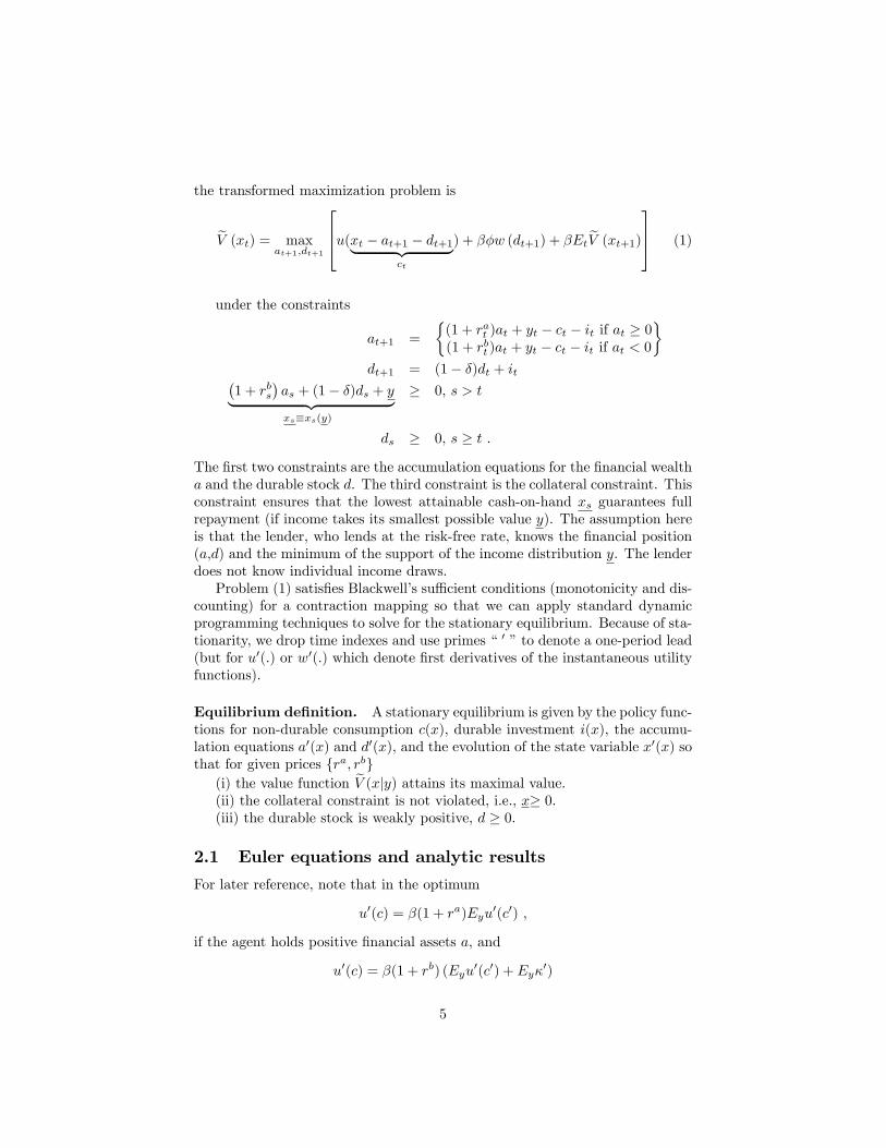
the transformed maximization problem is

eV (xt) = maxat+1;dt+1

264u(xt � at+1 � dt+1| {z }ct

) + ��w (dt+1) + �Et eV (xt+1)375 (1)

under the constraints

at+1 =

�(1 + rat )at + yt � ct � it if at � 0(1 + rbt )at + yt � ct � it if at < 0

�dt+1 = (1� �)dt + it�

1 + rbs�as + (1� �)ds + y| {z }xs�xs(y)

� 0, s > t

ds � 0, s � t .

The �rst two constraints are the accumulation equations for the �nancial wealtha and the durable stock d. The third constraint is the collateral constraint. Thisconstraint ensures that the lowest attainable cash-on-hand xs guarantees fullrepayment (if income takes its smallest possible value y). The assumption hereis that the lender, who lends at the risk-free rate, knows the �nancial position(a,d) and the minimum of the support of the income distribution y. The lenderdoes not know individual income draws.Problem (1) satis�es Blackwell�s su¢ cient conditions (monotonicity and dis-

counting) for a contraction mapping so that we can apply standard dynamicprogramming techniques to solve for the stationary equilibrium. Because of sta-tionarity, we drop time indexes and use primes � 0 �to denote a one-period lead(but for u0(:) or w0(:) which denote �rst derivatives of the instantaneous utilityfunctions).

Equilibrium de�nition. A stationary equilibrium is given by the policy func-tions for non-durable consumption c(x), durable investment i(x), the accumu-lation equations a0(x) and d0(x), and the evolution of the state variable x0(x) sothat for given prices {ra; rb}(i) the value function eV (xjy) attains its maximal value.(ii) the collateral constraint is not violated, i.e., x� 0.(iii) the durable stock is weakly positive, d � 0.

2.1 Euler equations and analytic results

For later reference, note that in the optimum

u0(c) = �(1 + ra)Eyu0(c0) ,

if the agent holds positive �nancial assets a, and

u0(c) = �(1 + rb) (Eyu0(c0) + Ey�

0)

5

if the agent holds debt and the collateral constraint is expected to bind so thatEy�

0 > 0. Because of the interest spread rb > ra, both Euler equations canbe slack. In this case the intertemporal rate of substitution of non-durableconsumption is in-between the lending and borrowing rate:

1 + ra <u0(c)

Eyu0(c0)< 1 + rb .

Then, agents hold zero �nancial assets, a = 0.In the optimum, durable investment is chosen so that it satis�es the condition

u0(c) = �Ey (u0(c0)(1� �) + �w0(d0) + (1� �)�0 + 0) ,

where 0 � 0 is the multiplier associated with the constraint d0 � 0 . As is intu-itive, the agent aligns the marginal utility of foregone non-durable consumptiontoday (resulting from durable investment) with the discounted marginal utilityderived from the durable tomorrow and the additional marginal utility of non-durable consumption that is a¤orded by re-selling the durable good (taking intoaccount its depreciation at rate �).Note that if the collateral constraint is expected to bind, Ey�0 > 0, present

consumption is valued less and more resources are transferred to the futureperiod. We can show the following

Remark 1: If utility is separable in the durable d and non-durable consumptionc, the instantaneous utility functions u(:) and w(:) are strictly concave, ofthe HARA family, and satisfy prudence so that u000(:) � 0 and w000(:) � 0,we can show:

(i) If the constraints are not binding, c(x), d(x) are concave, a(x) is convexand @c(x)=@x > 0, @d(x)=@x > 0. Moreover, @a(x)=@x � 0 if � = 1, andunder additional restrictions on concavity also for 0 � � < 1.

(ii) If the collateral constraint binds, @a(x)=@x falls and can become negative.

(iii) If the Euler equations for non-durable consumption are slack, c(x), d(x)can be locally strictly convex and a(x) can be locally strictly concave.

Proof: see the Appendix.

Remark 1(i) is an application of Theorem 1 in Carroll and Kimball (1996)to our model with durable and non-durable consumption. The concavity ofthe non-durable and durable consumption functions in models of incompletemarkets is very intuitive. Precautionary motives imply that the consumptionpropensity falls as agents have more cash-on-hand.The intuition for Remark 1(ii) is that the possibility of a binding collateral

constraint increases the amount of �nancial wealth a for small values of x sothat the slope is �atter. The optimality condition of borrowing agents

u0(c) = �(1 + rbt ) (Eyu0(c0) + Ey�

0)

6

illustrates that as Ey�0 falls with more cash-on-hand x (the collateral constraintis expected to be less binding), u0(c) decreases, ceteris paribus. The same holdsfor durable investment. The slope @a(x)=@x can be negative if the propensityof non-durable and durable consumption is larger than 1 and the collateralconstraint is relaxed as the durable stock increases.The intuition for Remark 1(iii) is that the propensity to consume out of cash-

on-hand has to increase if the Euler equations for non-durable consumption areslack since a0 = 0 and @a0=@x falls so that @a0=@x = 0. Hence, the consumptionpropensities increase since @c=@x + @d=@x = 1 if a0 = 0. The consumptionfunctions are no longer globally concave.Moreover, the durable stock increases relative to non-durable consumption

since the optimality conditions above (without multipliers for the constraints)imply

1 + ra < �(1� �) + ��Eyw0(d0)

Eyu0(c0)< 1 + rb .

The expected intra-temporal rate of substitution between durable and non-durable consumption tomorrow equals [1 + ra � �(1� �)] =(��) if the agentlends and

�1 + rb � �(1� �)

�=(��) if the agent borrows. Thus, as agents accu-

mulate cash-on-hand in the region where a0 = 0, Eyw0(d0)=Eyu0(c0) falls untilthe intra-temporal rate of substitution equals 1 + ra .The larger propensity for durable investment, for values of cash-on-hand x

where a0 = 0, is intuitive. As long as the depreciation rate is not too high,durables are an imperfect way to transfer resources intertemporally since therate of transformation is optimally in-between the exogenous interest factors1 + rb and 1 + ra.That �nancial market imperfections increase the propensity of durable and

non-durable consumption is supported by empirical evidence (see, for example,Alessie et al., 1997, for estimates using the period of �nancial deregulation inthe UK in the 1980s).3

2.2 Calibration and numerical results

Numerical algorithm. It is well known that problems like ours do not havea closed-form solution for optimal policies. Therefore, we pursue a numericalapproach which relies on value function iteration. While this allows us to con-veniently rely on the contraction properties of the Bellman operator, one of themain challenges for this technique is to �nd a way to get around the curse ofdimensionality. This is where the formulation of the problem that reduces thenumber of state variables to the minimum pays o¤ - by subsuming the portfoliopositions and the income realization in the single variable cash-on-hand. Hence,the state variables are cash-on-hand and the state of uncertainty, which is mod-eled as a 2-state Markov chain. The range of cash-on-hand, x, is restricted to

3Bertola et al. (2005) provide alternative microfoundations to explain the higher propensityfor durable purchases if there is an interest spread rb > ra and agents can be liquidityconstrained (a = 0). In this case, a monopolist dealer has an incentive to lower the creditprice of a durable good to attract liquidity constrained customers.

7

an interval [0; xmax]. We perform value function iteration on a grid over that in-terval. Our choice of xmax guarantees that, for every x and for every realizationof uncertainty, the equilibrium policy will imply a value for x tomorrow thatremains within that interval.4 We use linear interpolation of the value functionbetween these grid points.A feature of our algorithm that greatly enhances the accuracy of our solutions

is the fact that the maximizing choices for the policy (at each state and eachiteration) are not selected from a discretized set of choices, but rather by solvingthese maximization problems continuously over portfolio choices. We rely on anumerical optimization routine5 , which can also handle the collateral constraintand sign restrictions, to perform this task and to obtain the implicit multiplierson the constraints. The policy functions over the range [0; xmax] are obtainedfrom the optimal policy choices on the grid by interpolation, using cubic splines.As has become standard in the literature (see, e.g., Judd, 1992, and Aruoba

et al., 2006), we evaluate the accuracy of our solutions by the normalized Eulerequation errors implied by the policy functions. These are smaller than 4�10�4over the entire range where the Euler equations apply with equality, and infact much smaller for most values that the state variables of our problem canassume.

Calibration. We normalize average labor income y to 1, and parametrize theutility functions

u(c) =c1�� � 11� � and w(d) =

(d+ d)1�� � 1

1� � ,

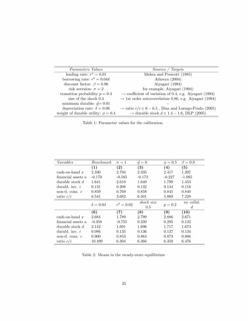
where, as mentioned above, d > 0 allows the consumer to hold no durable stock.We set risk aversion for the non-durable and durable good � = 2 which is wellwithin the range of commonly used values, and assume d= 0:01. It turns outthat this parameter is rather unimportant and can be set to negligibly smallvalues without changing the quantitative results much. This is because theregion of d close to zero is not important in our simulations. We calibrate thesize of the shocks and transition probabilities of our 2-state Markov chain as0:4. This implies a coe¢ cient of variation of 0:4 and a �rst-order autocorrelationof 0:86 which is within the range of reasonable values considered by Aiyagari(1994).We calibrate our model to the US, following previous calibrations by Diaz

and Luengo-Prado (2005) and Athreya (2004). Table 1 summarizes the cali-bration parameters. We calibrate the relative taste for the durable � and thedepreciation rate � so that we match a ratio of the durable stock to disposableincome of 1.6 and a ratio of non-durable consumption over durable investment

4 In our algorithm, we choose the grid for cash-on-hand so that for an upper bound of cash-on-hand x , the optimal policies imply that the maximal attainable cash-on-hand, x0max (forthe highest realization of income ymax) is smaller than this upper bound: x0max = (1 + r) a

0+ymax + (1� �) d0 < x. Using x = 0 as a lower bound gives us a compact state space (thisbound is implied by the collateral constraint).

5We are using the Matlab routine fmincon().

8

0 2 4 6 8-10

-5

0

5

cash-on-hand

Valu

e fu

nctio

n

0 2 4 6 8-2

0

2

4

cash-on-hand

Fina

ncia

l pol

icy

0 2 4 6 80.5

1

1.5

2

2.5

cash-on-hand

Dur

able

pol

icy

0 2 4 6 80

0.5

1

1.5

cash-on-hand

Non

-dur

. Con

sum

ptio

n po

licy

Figure 2: Value and policy functions in the good and bad state

slightly above 6 (see Diaz and Luengo-Prado, 2005, for the discussion of empir-ical estimates). This results in � = 0:4 and � = 0:08. The other parameters arerather standard and their sources are listed in Table 1.The choice of the depreciation rate merits further discussion. We need a

rather high depreciation rate so that a durable stock of 1.6, which is realisticempirically, is consistent with a ratio of non-durable consumption over durableinvestment of 6. Although a depreciation rate � = 0:08 is less realistic for hous-ing, the rate is below commonly assumed values for other important durableslike cars or computers. Thus, we view it as a reasonable approximation for thedepreciation of a durable composite. We will also present results for a lowerdepreciation rate � = 0:04 which is closer to commonly used depreciation ratesas used in Campbell and Hercowitz (2005).

Value function and policy functions. Figure 2 displays the solution for thevalue function and the policy functions in the bad and good income state. Thevalue function is smooth and concave. Not surprisingly, the function shifts downin the bad state of the world. The policy functions have a slightly non-standardshape consistent with the results of Remark 1. Because of the interest spreadrb > ra, a = 0 for an interval of cash-on-hand values. This local concavityof the �nancial policy implies local convexities in the policy functions for non-durable consumption and the durable stock. The local convexity is much morepronounced for the durable policy. This depends on whether the depreciationrate is low enough so that durables are a reasonably attractive vehicle to transfer

9

0 100 200 3000

1

2

t

c t0 100 200 300

0

5

t

x t

0 100 200 300-2

0

2

t

a t

0 100 200 3000

2

4

t

d t

0 100 200 3000.5

1

1.5

t

y t

0 100 200 300-1

0

1

t

i t

Figure 3: Time-series simulation of the economy without default

resources intertemporally.Note that the constraint d � 0 is never binding whereas the collateral con-

straint is expected to bind for values of cash-on-hand close to zero. We nowsimulate our economy to �nd out more about the mean and distribution of thepolicy variables in the steady state.

Simulations. We simulate our economy for 10,000 periods. Figure 3 displaysthe results for an arbitrarily chosen subsample of 300 periods. If the exogenousincome process yt implies a long enough sequence of bad-state incomes, the agentaccumulates �nancial debt as he borrows against the durable stock. If the badshocks persist, the agent might not have the resources to keep the durable stockat his current level so that it depreciates. This tightens the collateral constraintand can sometimes imply that x = 0. The collateral constraint xt � 0, however,is also important for behavior if x > 0, as long as the constraint is expected tobind.Note that without income uncertainty, the impatient consumer would always

be at his borrowing limit. Income uncertainty implies that the agent does notborrow as much and, if income is persistently good, he even accumulates somebu¤er-stock of assets, at > 0. Finally, we observe that durable investment ismore volatile than consumption also because of the high propensity to invest if�nancial assets are zero. We return to this point below.Table 2 displays the averages in the steady-state equilibrium for the main

variables of interest. In column (1) we display the results for our benchmark

10

economy. All values are expressed in average-income equivalents. On average,the consumer holds 2:3 of average income as cash-on-hand and borrows a sixthof average income with �nancial assets. The size of the durable stock of is 1:64and the ratio of non-durable consumption over durable investment is 6:5 which isin line with empirical evidence for the US (see Diaz and Luengo-Prado, 2005).6

Given that the income shocks are purely idiosyncratic, the law of large num-bers applies upon aggregation (see Uhlig, 1996) and the time-series distribu-tion can be used as an approximation of the cross-sectional distribution in thesteady state. Figure 4 displays such distributions for non-durable consumptionc, durable holdings d, �nancial assets a, and cash-on-hand x. The density ofcash-on-hand is bell-shaped and is truncated at x = 0, where collateral con-straints bind. Thus, also the densities of c, d, and a have more mass at theirlower bound of the support. Moreover, �nancial assets have a mass point ata = 0 when the (non-durable) consumption Euler equation is slack for both ra

and rb. The frequency of agents with zero �nancial assets in Figure 4 is 11.7%.This is about the same order of magnitude as the 10% of US consumers be-tween age7 25 and 50 which hold net non-housing wealth in the range from zeroto two weeks�of their permanent income (see the discussion of these statisticsbased on the 1995 Survey of Consumer Finances in Carroll, 2001). The higherpropensity to consume in the range where a = 0 implies that both the distribu-tion for non-durable consumption and durable holdings are bimodal. Consistentwith the much stronger change in the propensity to purchase durables observedin Figure 2, the bimodality is more pronounced for the distribution of durableholdings.

Changes in parameters. We now investigate how changes of the model�s pa-rameters alter the steady-state equilibrium. In Table 2, column (2), we computethe average equilibrium for lower risk-aversion, � = 1. This reduces non-durableconsumption and induces accumulation of cash-on-hand in terms of durables.Thus, the collateral constraint is laxer and consumers borrow more when badincome shocks occur.In column (3) we investigate whether the parameter d is important in our

benchmark equilibrium. We set d = 0 and �nd no signi�cant changes. As ex-pected durable holdings increase slightly compared to non-durable consumptionbecause the marginal utility derived from the durable is higher (for a given d).Thus, the ratio c=i falls. The larger durable stock also relaxes the collateral con-straint. This allows agents to borrow more so that the average �nancial-assetposition is lower. The increase in debt is not enough, however, to completelyo¤set the increase in d so that cash-on-hand increases. The e¤ect of increasing� from 0:4 to 0:5 is qualitatively the same (see column (4)).If agents are more impatient (� = 0:9), the consumers borrow more (see

column (5)). At the same time the ratio c=i increases since non-durable con-

6Note that average disposable income y + rja is nearly equal to average income sincerja ' 0 .

7Bu¤er-stock saving behavior should matter for consumers in this age range.

11

0 0.5 1 1.50

500

1000

1500

Non-dur. consumption

Den

sity

0 1 2 30

500

1000

1500

2000

Durable holdings

Den

sity

-2 0 2 40

1000

2000

3000

Financial assets

Den

sity

0 5 100

500

1000

1500

Cash-on-hand

Den

sity

Figure 4: The steady-state distributions

sumption generates utility today whereas durable investment only generatesutility tomorrow. Thus, the durable stock falls which also tightens the collat-eral constraint. Since consumers borrow more, the collateral constraint bindsmuch more often.When calibrating the model, we have mentioned that a depreciation rate

� = 0:08 is rather high. In column (6) we lower the depreciation rate to � =0:04. This increases the durable stock and non-durable consumption and lowersdurable investment which is only a tenth of non-durable consumption. Thelarger cash-on-hand relaxes the collateral constraint and allows agents to borrowmore in bad times so that the average �nancial asset position is lower.If we lower the borrowing rate rb to 0:02, not surprisingly agents borrow

more (see column (7)). Cheaper borrowing also allows consumers to a¤ord alarger durable stock. Total cash-on-hand decreases, however, because of moreconsumer debt. The fall in the borrowing rate also reduces the spread in the�nancial market so that agents hold zero �nancial assets less frequently andthe kinks in the policy functions of durables and �nancial assets become lesspronounced. This implies that the frequency of consumers with �nancial assetsa = 0 is 2.3% which is similar to the empirically observed frequency of 2.5% forconsumers holding precisely zero net non-housing worth in the 1995 Survey ofConsumer Finances in the US (see Carroll, 2001). The lower frequency impliesin our model that the distribution of durable holdings becomes less bimodal(the �gures are not reported but are available upon request).

12

3 Income risk and household debt

We now apply our model to answer the question whether higher income risk isa good candidate for explaining the rise in household debt in the US in the lastdecades. We �nd that in our model the answer is no. The reason is that higherrisk (in terms of shock size or persistence) increases the bu¤er-stock motiveand thus decreases the debt holdings of agents. Instead, institutional �nancialmarket reforms that allow consumers to collateralize more of their debt are amore plausible explanation in our model.The results are in Table 2, columns (8)-(10). In column (8) we increase

the size of shocks from 0:4 to 0:5, which implies an increase of the standarddeviation of log-income by 12%. This is much more than the increase of thecross-sectional variance of earnings in the US (15 basis points in the periodbetween 1981 and 2003) to illustrate the point qualitatively. As can be seenin column (8), consumers hold more �nancial assets as bu¤er stock and also,conditional on holding debt, average debt increases from �0:35 to �0:22. Theaverage durable stock increases slightly. The results are qualitatively the same ifthe shocks are more persistent (see column (9) where the transition probabilityfalls from p = 0:4 to p = 0:2). Moreover, the equilibrium change is similar if weexogenously tighten the collateral constraint in column (10) where we no longerallow consumers to collateralize their durable stock. Thus, relaxing collateralconstraints, does increase consumer debt. The bottom-line is that an increasein income risk does not increase consumer debt if the bu¤er-stock saving motiveis strong. Instead, lower collateral requirements are a possible explanation forhigher consumer debt (see Campbell and Hercowitz, 2005, for a discussion onhow market innovations that followed the Monetary Control Act of 1980 andthe Garn-St.Germain Act of 1982 relaxed collateral constraints on householddebt in the US).However, we cannot fully dismiss the hypothesis that more idiosyncratic

income risk increased consumer debt for at least two reasons:(i) In our partial-equilibrium model interest rates are exogenous. A general

equilibrium e¤ect as in Aiyagari (1994) would imply that interest rates haveto fall until the asset market clears. This would reduce the bu¤er-stock savingmotive. However, the results in Aiyagari suggest that it is unlikely that thegeneral equilibrium e¤ect outweighs the direct partial-equilibrium e¤ect.(ii) The access to borrowing and idiosyncratic risk maybe endogenously

related. For example in Krueger and Perri (2005), limited enforcement ofcredit contracts implies that �nancial market development interacts with incomevolatility. If more volatile income makes the exclusion from credit markets incase of default more costly, this might foster �nancial market development. Inthis case, more volatile income will induce a higher bu¤er-stock but with respectto a laxer borrowing limit. Whether this implies more or less debt depends onwhich e¤ect dominates quantitatively and is a priori unclear.

13

4 Conclusion

We set up and solve a heterogenous-agent model with incomplete markets inwhich households derive utility from non-durable consumption and durable hold-ings. We show that an interest spread between the borrowing and lending rateimplies local convexities in the policy functions for non-durable consumptionand especially durable holdings which are important quantitatively.We apply our model to the question whether an increase in income risk can

explain the increase in household debt observed in many developed countries inthe past decades. Calibrating our model to the US economy, we �nd that anincrease in income risk reduces average household debt, also if we condition onthose consumers who hold some debt. Thus, our model with bu¤er-stock savingmotives has di¤erent predictions than models which analyze approximationsaround a non-stochastic steady state (see, for example, Iacoviello, 2005). Weargue that an increase in idiosyncratic income risk alone cannot explain theincrease in household debt in the US and other developed countries.In current research we extend our model to analyze interactions between ag-

gregate and idiosyncratic risk and whether the observed decrease of aggregaterisk in the US has facilitated the risk-sharing provided by �nancial intermedi-aries.

Appendix

Proof of Remark 1The proof is based on results of Carroll and Kimball (1996).Claim (i): If the constraints are not binding, c(x), d(x) are concave and

a(x) is convex and @c(x)=@x > 0, @d(x)=@x > 0, @a(x)=@x � 0 .Proof: We want to show that if u(:) and w(:) are HARA utility functions

and u0(:) > 0, u00(:) < 0, u000(:) � 0, and w0(:) > 0, w00(:) < 0, w000(:) � 0, thenc(x), d(x) are concave and a(x) is convex and @c(x)=@x > 0, @d(x)=@x > 0,@a(x)=@x � 0 .Our problem is

eVt (xt) = maxat+1;dt+1

264u(xt � at+1 � dt+1| {z }ct

) + ��w (dt+1) + �Et eVt+1 (xt+1)375

where xt � (1 + rj)at + yt + (1� �)dt so that the budget constraint

ct = xt � at+1 � dt+1 .

To start we also assume a �nite horizon so that we have the terminal condi-tion

cT = xT .

14

We then proceed analogously as in Carroll and Kimball and prove Lemmas1-3. For this we de�ne as �t((1+r

j)at+1(xt)+(1��)dt+1(xt)) � �Et eVt+1 (xt+1),where

xt+1 � (1 + rj)at+1 + yt+1 + (1� �)dt+1.

Note that �t(:) is written as a function of choice variables.The �rst lemma shows that the property of prudence is conserved when

aggregating across states of nature.

Lemma 1: If eV 000t+1 eV 0t+1= heV 00t+1i2 � k, then �000t �0t= ��00t �2 � k .Proof: see Carroll and Kimball, p. 985.The second lemma shows that the property of prudence is conserved when

aggregating intertemporally.

Lemma 2: If �000t �0t=��00t�2 � k and u000u0= [u00]2 � k, w000w0= [w00]2 = k, theneV 000t eV 0t = heV 00t i2 � k .

Proof: Following Carroll and Kimball, p. 985/986, we denote the marginalutility of non-durable consumption at the optimal consumption level with zt =u0(c�t (xt). Neglecting the collateral constraint and interest spread, we know thatin our problem the following equations hold in the optimum:

zt = u0(c�t (xt)) ,

u0(c�t (xt)) = eV 0t (xt) ,u0(c�t (xt)) = �(1 + rj)Et eV 0t+1 (xt+1) = (1 + rj)�0t ,u0(c�t (xt)) = ��w0(dt+1) + (1� �)�0t ,

where �t((1+rj)at+1(xt)+(1��)dt+1(xt)) . We then de�ne the functions ft(zt),

gt(zt), ht(zt), lt(zt) asft(zt) = u

0�1(zt) = ct ,

ht(zt) = eV 0�1t (zt) = xt ,

lt(zt) = w0�1�zt � (1� �)�0t(:)

��

�= dt+1 ,

gt(zt) = �0�1t

�zt

1 + rj

�� (1� �)lt(zt) = (1 + rj)at+1 .

Noting from the last equation that

(1 + rj)at+1 + (1� �)dt+1 = �0�1t

�zt

1 + rj

�,

15

we use this expression in as the argument of �0t(:) in the second equation whichthen simpli�es to

lt(zt) = w0�1�

rj + �

�� (1 + rj)zt

�= dt+1

Dropping time indexes for functions f , g, l, h, we have

f 0(z) =1

u00(c(z)),

f 00 = � u000(c)

[u00(c)]2 f 0|{z}@c=@z

= � u000

[u00]3 ,

so that

�zf00

f 0=u000u0

[u00]2 � k .

Similarly,

�zh00

h0=eV 000t eV 0theV 00t i2 .

Furthermore,

l0 =rj + �

�� (1 + rj)w00,

l00 = ��rj + �

�w000

�� (1 + rj) [w00]2 l0 ,

so that

�zl00

l0=w000w0

[w00]2 � k ,

where we use thatrj + �

�� (1 + rj)zt = w

0(dt+1) .

Finally,

g0 =1

(1 + rj)�00��0�1t

�zt

1+rj

�� � (1� �) rj + �

�� (1 + rj)w00,

g00 = � �000

(1 + rj)2��00�3 + (1� �)

�rj + �

�w000

�� (1 + rj) [w00]2 l0 .

Thus,

�zg00

g0=

�000�0

(1+rj)[�00]3� (1� �)w000w0

[w00]2l0

1(1+rj)�00 � (1� �)l0

.

16

For � = 1, this simpli�es to

�zg00

g0=�000�0��00�2 � k ,

For 0 < � < 1,

�zg00

g0=

g0

g0 � (1� �)l0�000�0��00�2 � (1� �)l0

g0 � (1� �)l0w000w0

[w00]2 .

If we assume HARA utility so that w000w0= [w00]2 = k, then �000t �0t=��00t�2 � k

implies that

�zg00

g0� g0

g0 � (1� �)l0 k �(1� �)l0

g0 � (1� �)l0 k = k .

Now note that sincect = xt � at+1 � dt+1

andat+1 =

g

(1 + rj)� (1� �)l ,

we have

h = f +g

(1 + rj)� (1� �)l + l

= f +g

(1 + rj)+ �l .

That is, h is an additive function of f , g and l, so that

h0 = f 0 +g0

(1 + rj)+ �l0

and

h00 = f 00 +g00

(1 + rj)+ �l00 .

This implies that

�zh00

h0= �z

f 00 + g00

(1+rj) + �l00

f 0 + g0

(1+rj) + �l0

=f 0

f 0 + g0

(1+rj) + �l0| {z }

>0

��zf

00

f 0

�| {z }

�k

+

g0

(1+rj)

f 0 + g0

(1+rj) + �l0| {z }

>0

��zg

00

g0

�| {z }

�k

+�l0

f 0 + g0

(1+rj) + �l0| {z }

>0

��zl

00

l0

�| {z }

�k

� k ,

17

since this is a weighted average of expressions that are larger or equal than k.

As in Carroll and Kimball we move on to show Lemma 3, where we exploitagain that HARA utility implies w000w0= [w00]2 = k and u000u0= [u00]2 = k withequality.

Lemma 3: If eV 000t eV 0t = heV 00t i2 � k, w000w0= [w00]2 = k and u000u0= [u00]2 = k, thenthe optimal consumption policy rules c(x) and d(x) are concave and liquidassets a(x) are convex.

Proof: Note thatct(x) = ft(h

�1t (x)) .

Thus,@c

@x=f 0(h�1)

h0(h�1)=eV 00u00

> 0

if u00 < 0, eV 00 < 0 and@2c

@x2=

�f 00(h�1)=h0(h�1)

� �h0(h�1)

���f 0(h�1)

� �h00(h�1)=h0(h�1)

�[h0(h�1)]

2

=f 0(h�1)

[h0(h�1)]2

�f 00(h�1)

f 0(h�1)� h

00(h�1)

h0(h�1)

�.

Applying Lemma 2 we �nd

@2c

@x2=

f 0(h�1)

[h0(h�1)]2

1

z

26664�zh00(h�1)h0(h�1)| {z }�k

� �zf00(h�1)

f 0(h�1)| {z }=k

37775 .

The sign of this derivative is smaller or equal than zero if sgn(f 0(h�1)) < 0.Recalling that f 0(h�1) = f 0(z) = 1=u00 < 0, this is the case for a strictlyconcave utility function. Analogous manipulations for dt(x) = lt(h

�1t (x)) prove

@d(x)=@x > 0 and @2d(x)= (@x)2 � 0.Since at+1(x) = xt � ct(x)� dt+1(x),

@a

@x= 1� @c(x)

@x� @d(x)

@x

and@2a

@x2= �@

2c(x)

@x2� @

2d(x)

@x2� 0.

Thus, �nancial wealth increases or decreases with x, depending on whetherthe marginal propensity to consume @c(x)=@x + @d(x)=@x R 1. The secondderivative is certainly positive so that a(x) is convex.

18

We now investigate the properties of the consumption propensities further.In particular, do we know whether @c(x)=@x+ @d(x)=@x > 1?Noting that

h0 = f 0 +g0

(1 + rj)+ �l0

we can write@c

@x=

f 0(h�1)

f 0(h�1) + g0(h�1)(1+rj) + �l

0(h�1)

and@d

@x=

l0(h�1)

f 0(h�1) + g0(h�1)(1+rj) + �l

0(h�1).

Thus,@c

@x+@d

@x=

f 0(h�1) + l0(h�1)

f 0(h�1) + g0(h�1)(1+rj) + �l

0(h�1)< 1 ,

if � = 1 and g0(h�1) > 0 .

We now compute the derivative of a(x) = g(h�1(x))=�1 + rj

�:

@a

@x=

1

1 + rjg0(h�1(x))=h0(h�1(x))

=eV 00t

1 + rj

�1

(1 + rj)�00� (1� �) rj + �

�� (1 + rj)w00

�,

which is certainly positive if � = 1 since eV 00t < 0; �00 < 0. For � < 1, we need toimpose an additional condition on the curvature

1

(1 + rj)�00� (1� �) rj + �

�� (1 + rj)w00< 0 or

�00

��w00<

rj + �

1� � .

In general the sign of @a=@x depends on the relative curvature of the value func-tion expected tomorrow, �00t , and instantaneous utility derived from the durable,w00. Intuitively, a larger � makes durables less useful to transfer utility and thusincrease the marginal propensity of �nancial assets to transfer resources.

The lemmas derived above imply Theorem 1 as in Carroll and Kimball(1996). Note that the second-order derivatives for the policy functions holdwith strict equality if k > 0 and there is some labor income uncertainty.Carroll and Kimball show results for a �nite horizon. In a �nite horizon, we

have that in the last period VT = u(c) + �w(d) so that prudence of u(:) andw(:) trivially also apply to VT . Then one iterates forward using using Lemma

19

1 and 2. To extend these results to the in�nite horizon one needs to applythe contraction property of V , for T !1. Since cash on hand is �nite, agentsdiscount and V satis�es monotonicity, limT!1 Vt(x) = V (x) for all x (see Lucasand Stokey, 1989, ch. 3). Pointwise convergence implies that the properties ofVt are conserved as Vt converges towards V . �

Claim (ii): If the collateral constraint binds, @a(x)=@x falls and can becomenegative.Proof: Intuitively, the value function will be more concave if the collateral

constraint holds. The expression for the propensities derived above, then implythat @c(x)=@x+@d(x)=@x increases if eV 00 falls (i.e., increases in absolute value).This can imply @a(x)=@x < 0, which we now want to derive more formally.Adding the multiplier � for the collateral constraint and for the constraintd > 0, the four equations used in Lemma 2 change to

zt = u0(c�t (xt) ,

u0(c�t (xt) = eV 0t (xt) ,u0(c�t (xt) = (1 + rj)

��0t + Et�

�,

u0(c�t (xt) = ��w0(dt+1) + (1� �)��0t + Et�

�+ Et ,

so thatft(zt) = u

0�1(zt) = ct ,

ht(zt) = eV 0�1t (zt) = xt ,

lt(zt) = w0�1

zt � (1� �)

��0t(:) + Et�

�� Et

��

!= dt+1 ,

gt(zt) = �0�1t

�zt

1 + rj� Et�

�� (1� �)lt(zt) = (1 + rj)at+1 .

Observing that

(1 + rj)at+1 + dt+1 = �0�1t

�zt

1 + rj� Et�

�,

the third equation can be rewritten as

lt(zt) = w0�1

rj+�1+rj zt � Et

��

!= dt+1 .

Thus, a expectedly binding collateral constraint does not directly a¤ect dt+1 .Instead if the constraint d = 0 is expected to bind this lowers w0(dt+1) and thusinduces a larger dt+1, ceteris paribus.More interestingly, let us investigate how the marginal propensity of a(x)

changes if the collateral constraint is binding (we neglect the constraint d � 0for simplicity). Recall that a(x) = g(h�1(x))=

�1 + rj

�:

20

@a

@x=

1

1 + rjg0(h�1(x))=h0(h�1(x))

=eV 00t

1 + rj

1

1+rj � Et@�@z

�00� (1� �) rj + �

�� (1 + rj)w00

!.

Since a larger z = u0(c�(x)) means a smaller c and x, Et@�=@z > 0, i.e. thecollateral constraint is expected to become more binding for smaller x and thuslarger z. Then, this derivative shows that the propensity @a=@x falls if thecollateral constraint is expected to bind. In particular, the propensity need nolonger be positive. The intuition is that the possibility of a binding collateralconstraint increases the amount of �nancial wealth for small values of x so thatthe slope is �atter. �

Claim (iii): If the Euler equations for non-durable consumption are slack,c(x), d(x) can be locally strictly convex and a(x) can be locally strictly concave.Proof: We show that c(x), d(x) are locally strictly convex and a(x) is lo-

cally strictly concave in the range where a = 0. In particular, @c(x)=@xja=0 >@c(x)=@x and @d(x)=@xja=0 > @d(x)=@x for given x, and Eyw0(d0)=Ey�0 falls.

If at+1(x) = 0,ct = xt � dt+1

and thush = f + l .

Hence,

�zh00

h0=

f 0

f 0 + l0| {z }>0

��zf

00

f 0

�| {z }

�k

+l0

f 0 + l0| {z }>0

��zl

00

l0

�| {z }

�k

so that the curvature of w(:) becomes much more important for the curvatureof the value function. Also

@c

@x+@d

@x=f 0(h�1) + l0(h�1)

f 0(h�1) + l0(h�1)= 1 ,

so that the propensities increase since @a(x)=@x > 0 to the left of the rangewhere a(x) = 0. The local increase of the propensities implies local convexityof the consumption functions. Moreover, @a(x)=@x > 0 is locally concave.

More formally, if @a(x)=@x = 0, the collateral constraint is certainly notbinding and

21

zt = u0(c�t (xt) ,

u0(c�t (xt) = eV 0t (xt) ,(1 + ra)�0t < u0(c�t (xt) < (1 + r

b)�0t

u0(c�t (xt) = ��w0(dt+1) + (1� �)�0t ,

so thatft(zt) = u

0�1(zt) = ct ,

ht(zt) = eV 0�1t (zt) = xt ,

lt(zt) = w0�1�zt � (1� �)�0t(:))

��

�= dt+1 ,

gt(zt) = �0�1t (zt + �

b)� (1� �)lt(zt) = (1 + rb)at+1or

gt(zt) = �0�1t (zt � �a)� (1� �)lt(zt) = (1 + ra)at+1

with �a > 0 and �b > 0.This implies

@a

@x=

1

1 + rbg0(h�1(x))=h0(h�1(x))

=eV 00t

1 + rb

1 + @�b

@z

(1 + rb)�00� (1� �) rb + �

�� (1 + rb)w00

!.

For the range at+1(x) = 0 , @�b=@z < 0 so that @a=@x = 0 (Note that @�b=@x >

0.). Similarly, for the lending Euler-equation,

@a

@x=

eV 00t1 + rb

1� @�a

@z

(1 + rb)�00� (1� �) rb + �

�� (1 + rb)w00

!,

with @�a=@z > 0 (Note that @�a=@x < 0.). �

References

[1] Aiyagari, S. Rao (1994): �Uninsured Idiosyncratic Risk and AggregateSavings�, Quarterly Journal of Economics, vol. 109, 659-84.

[2] Alessie, Rob, Michael P. Devereux, and Guglielmo Weber (1997) �Intertem-poral Consumption, Durables and Liquidity Constraints: A cohort analy-sis,�European Economic Review, 41:1, 37-59.

22

[3] Araujo, Aloiso, Mario R. Pascoa and Juan P. Torres-Martinez (2002): �Col-lateral Avoids Ponzi Schemes in Incomplete Markets�, Econometrica, vol.70, 1613-38.

[4] Aruoba, Boragan, Jesús Fernández-Villaverde and Juan Rubio-Ramírez(2006): �Comparing Solution Methods for Dynamic EquilibriumEconomies�, Journal of Economic Dynamics and Control, forthcoming.

[5] Athreya, Kartik (2005): �Fresh Start or Head Start? Uniform BankruptcyExemptions and Welfare�, Journal of Economic Dynamics and Control,forthcoming.

[6] Bertola, Giuseppe, Stefan Hochgürtel and Winfried Koeniger (2005):�Dealer Pricing of Consumer Credit�, International Economic Review, vol.46, 1103-42.

[7] Campbell, Je¤rey R. and Zvi Hercowitz (2005): �The Role of CollateralizedHousehold Debt in Macroeconomic Stabilization�, NBER Working PaperNo. 11330.

[8] Carroll, Christopher D. (1997): �Bu¤er-Stock Saving and Life Cy-cle/Permanent Income Hypothesis�, Quarterly Journal of Economics, vol.112, 1-55.

[9] Carroll, Christopher D. (2001): �A Theory of the Consumption Func-tion, With andWithout Liquidity Constraints (Expanded Version)�, NBERWorking Paper No. 8387.

[10] Carroll, Christopher D. and Miles Kimball (1996): �On the Concavity ofthe Consumption Function�, Econometrica, vol. 64, 981-92.

[11] Deaton, Angus (1991): �Saving and Liquidity Constraints�, Econometrica,vol. 59, 1221-48.

[12] Deaton, Angus and Guy Laroque (1992): �On the Behavior of CommodityPrices�, Review of Economic Studies, vol. 59, 1-23.

[13] Diaz, Antonia and Maria J. Luengo-Prado (2005): �Precautionary Savingsand Wealth Distribution with Durable Goods�, Northeastern University,mimeo.

[14] ECRI (2000): �Consumer Credit in the European Union,�ECRI ResearchReport No. 1, Brussels.

[15] Gruber, Joseph W. and Robert F. Martin (2003): �Precautionary Savingsand the Wealth Distribution with Illiquid Durables�, Board of Governors ofthe Federal Reserve System, International Finance Discussion Papers No.773.

[16] Iacoviello, Matteo (2005): �Household Debt and Income Inequality, 1963-2003�, Boston College, mimeo.

23

[17] Judd, Kenneth (1992): �Projection Methods for Solving Aggregate GrowthModels�, Journal of Economic Theory, 58, 410-452.

[18] Krueger, Dirk and Fabrizio Perri (2005): �Does Income Inequality Leadto Consumption Inequality? Evidence and Theory�, Review of EconomicStudies, forthcoming.

[19] Mehra, Rajnish and Edward C. Prescott (1985): �The Equity Premium: apuzzle�, Journal of Monetary Economics, vol. 15 , 145-61.

[20] Uhlig, Harald (1996): �A Law of Large Numbers for Large Economies�,Economic Theory, vol. 8, 41-50.

[21] Waldman, Michael (2003): �Durable Goods Theory for Real World Mar-kets�, Journal of Economic Perspectives, vol. 17, 131-54.

24

Parameters Values Sources / Targetslending rate: ra = 0:01 Mehra and Prescott (1985)

borrowing rate: rb = 0:044 Athreya (2004)discount factor: � = 0:96 Aiyagari (1994)risk aversion: � = 2 for example, Aiyagari (1994)

transition probability p = 0:4 ! coe¢ cient of variation of 0:4, e.g. Aiyagari (1994)size of the shock 0:4 ! 1st order autocorrelation 0:86, e.g. Aiyagari (1994)

minimum durable: d= 0:01 -depreciation rate: � = 0:08 ! ratio c=i 2 6� 6:5 , Diaz and Luengo-Prado (2005)

weight of durable utility: � = 0:4 ! durable stock d 2 1:4� 1:6, DLP (2005)

Table 1: Parameter values for the calibration.

Variables Benchmark � = 1 d = 0 � = 0:5 � = 0:9(1) (2) (3) (4) (5)

cash-on-hand x 2.330 2.794 2.335 2.417 1.207�nancial assets a -0.170 -0.585 -0.172 -0.227 -1.085durable stock d 1.641 2.610 1.649 1.799 1.453durabl. inv. i 0.131 0.208 0.132 0.144 0.116non-d. cons. c 0.859 0.769 0.858 0.845 0.840ratio c=i 6.541 3.682 6.501 5.869 7.228

� = 0:04 rb = 0:02shock size

0:5p = 0:2

no collat.d

(6) (7) (8) (9) (10)cash-on-hand x 2.684 1.789 2.799 2.886 2.671�nancial assets a -0.358 -0.755 0.239 0.295 0.132durable stock d 2.142 1.691 1.696 1.717 1.673durabl. inv. i 0.086 0.135 0.136 0.137 0.134non-d. cons. c 0.900 0.853 0.864 0.873 0.866ratio c=i 10.499 6.304 6.366 6.359 6.476

Table 2: Means in the steady-state equilibrium

25