income poor or calorie poor? who should get the subsidy?
TRANSCRIPT
1 | P a g e
Income Poor or Calorie Poor? Who should get the Subsidy?
Chandana Maitra1, Sriram Shankar2 and D.S. Prasada Rao3
Abstract: Poverty-nutrition linkage remains somewhat puzzling for India because trends in
calorie poverty and income poverty have been moving in opposite directions in the Indian
economy for the past few decades. Given the above, this paper explores the question whether
income poverty increases the risk of calorie poverty in cross section context, using data from
a random survey of 500 slum households of Kolkata in 2010-11. Calorie poverty is estimated
using household specific calorie norm accounting for age, gender and activity status of
household members. To address the issue of causality in cross section data, appropriate
empirical models such as simultaneous probit and Bayesan propensity score matching are
used. Results indicate, an income poor household is at greater risk of being calorie poor.
However, there is lack of one-to-one correspondence between the two groups of households.
Additionally, transitional households just above the poverty line exhibit very different calorie
behaviour. Findings imply, subsidies offered to income poor households should ameliorate
calorie poverty. Moreover, subsidies should be directed to income poor rather than calorie
poor households. Additionally, nutrition policy should have different prescription for
transitional households immediately above the poverty line. (188 words)
Key words: Nutrition policy, calorie poverty, income poverty, activity status, cross section,
endogeneity, simultaneous probit, Bayesian.
1 School of Economics, The University of Queensland, St Lucia, Brisbane, Australia. 2 Research School of Economics & ANU, Centre for Social Research and Methods, The Australian National
University, Canberra, Australia. 3 School of Economics, The University of Queensland, St Lucia, Brisbane. Australia.

2 | P a g e
1 Introduction
The poverty-nutrition linkage apparently seemed quite straightforward at one point of time.
Quoting Osmani (1992, page 1), “The study of poverty is….very much a study of the
people’s state of nutrition.” However, the puzzles in the relationship started surfacing when
two of the world’s largest transitioning economies today — India and China — began
experiencing a peculiar phenomenon whereby rising real income is accompanied by declining
calorie consumption. The peculiar trend has been observed in India since the late eighties
(Mehta and Venkatraman 2000; Chandrashekhar and Ghosh 2003; Rao 2000; Sen 2005;
Deaton and Dreze 2009; Li and Eli 2012; Gaiha et al.2010; Basu and Bansole 2012) and in
China between 1985 and 1992 (see Du et al. 2004), given the fact that most other developing
economies have experienced rising calorie intake in similar level of technological and
economic transformations. Following Patnaik (2010; cited in Smith 2013, page 7), stagnant
or declining calorie consumption during periods of economic growth are a rare phenomenon
and is unusual not just in the context of international trends but also in relation to India’s
own earlier experience. With economic growth, Indian households have moved up the Engel
curve, but the Engel Curve has fallen: on balance the consumption of calories and all other
nutrients has fallen in India over the last few decades (Banerjee and Dufflo 2011a). The
above phenomenon has been mirrored in prevalence of undernourishment moving in a
direction opposite to that suggested by income poverty signifying that calorie poverty may
not be a problem of income poor households alone (Palmer Jones and Sen, 2001;
Radhakrishna, 2005; Meenakhshi and Viswanathan, 2003; Ray and Lancaster, 2005;
Suryanarayan and Silva, 2007; Deaton and Dreze, 2009). This leads us rethink whether study
of poverty is a study of nutrition indeed.
3 | P a g e
One way of investigating the issue is to look at the question of whether income poverty leads
to calorie poverty at the household level in a cross section context. There’s sufficient
evidence in the literature at the cross section level that increase in income leads to improved
calorie intake (Strauss and Thomas, 1990; Bouis an Haddad, 1992; Gibson and Rozelle,
2002; Roy, 2001). A major fraction of this literature, including several studies on India
(Subranmanian and Deaton, 1996; Viswanathan and Meenakshshi, 2006, Deaton and Dreze,
2009), report positive calorie-expenditure elasticity.4 But there has been less rigorous
investigation, and hence less conclusive evidence on the question of whether income poverty
leads to calorie poverty as well in cross section data. The Indian experience will tell us that
the two phenomena may not be equivalent. Therefore the nexus between income poverty and
calorie poverty deserves separate inquiry and this is precisely the issue we attempt to address
in the present paper.
Given the above backdrop, we pose the question, ‘Does the probability of being income-poor
influence the probability of being calorie-poor?’ The hypothesis we test is: income poor and
calorie poor households may not be the same. The answer to this question is important in the
context of formulating nutrition-related policies. First, if the income poor and calorie poor are
different groups of households who should be the target of food subsidies? Moreover,
following Suryanaryan and Silva (2007), in targeting the poor public policy might lose sight
of the calorie poor households who are part of the above-poverty line group of households
and who will remain out of the domain of government subsidies if only the poor are targeted.
Secondly, if calorie shortfall is not a poverty driven phenomenon then would income-based
subsidy be a relevant policy at all in addressing nutritional deprivation. The question also
4 However, some studies do not find any evidence of income influencing demand for calorie (Behrman and
Deolalikar, 1987).

4 | P a g e
becomes pertinent in view of observations such as the extremely poor do not seem to be as
hungry for additional calories as one might expect (Banerjee and Duflo, 2007, page 5).
We attempt to answer the above question on the basis of the information collected from a
random sample of 500 households in slums of Kolkata. The reason we choose an urban
sample is urbanisation is emerging as an increasing threat to food security, in India as in
many other developing nations (FAO, 2008), yet urban food security is still relatively less
researched (Maxwell, 1999). The urban dynamics of food security are distinctly different
from those in rural areas and manifest themselves as lack of access to food primarily at the
household level (Ruel et al., 1998), resulting in the relative invisibility of chronic urban food
insecurity, to researchers and policy makers alike.
In addition to addressing the gaps in the literature with respect to the above concerns, our
paper has two significant methodological contributions. First, we identify a household as
calorie poor with respect to a household specific norm, following Viswanathan and
Meenakhshi (2006), by taking account of age, gender and activity status of each member of
the household. Following Viswanathan and Meenakhshi (2006) we believe this to be a
superior means of measuring calorie poverty as opposed to measuring it using a single per
capita norm which most other studies have done, when food intake data are available at the
household- (but not individual-) level.
Second, we recognize the possibility of endogeneity in our variables of interest – income
poverty and calorie poverty. The same unobservable factors that influence income poverty
are likely to influence calorie shortfall too. Another possible source of endogeneity is
measurement error — calorie and expenditure data being calculated from the same source
(see Srinivasan, 1981; Subramanian and Deaton, 1996).

5 | P a g e
In conducting the above exercises, we exploit the flexibility of models like simultaneous
probit (Maddala 1983; Greene, 2012) with further application of techniques like Bayesian
Propensity Score Matching (BPSM) for robustness (An 2010). In the absence of availability
of panel data with regard to our variables of interest, we restrict our analysis to the cross
section sample mentioned above. Since it is difficult to address causality in cross section data
when data is not generated out of a randomized control trial (RCT), we hope sound
techniques such as BPSM can mitigate this concern to a considerable extent. Use of Bayesian
is also justified because of its superiority over conventional PSM (Abadie and Imbens, 2008;
Alvarez and Levin, 2014).
The results indicate that income poverty increases the risk of being calorie poor. However,
there is a lack of one to one correspondence between the two variables since we note the
presence of a large fraction of calorie poor households among the set of non-poor households.
Additionally, separate policy prescription is warranted for transitional households just above
poverty line who exhibit very different calorie behaviour compared to the rest.
The rest of the paper is organized as follows. Section 2 describes the theoretical framework,
Section 3 and 4 outlines method including data and statistical analysis, Section 4 reports
results, Section 5 discusses the results and Section 6 concludes with policy implications and
suggested direction of future research.
2 Theoretical Framework
Calorie demand is estimated within the framework of consumer demand theory by
incorporating the demand for characteristics (Lancaster 1966) with a household production
theory (Becker 1965). Drawing from (Rose et al. 1998), one can consider a utility function
6 | P a g e
that has vectors of taste components, S, and nutrients, N, found in meals, as well as goods,
𝑋0 and leisure, represented by L:
𝑈 = 𝑈(𝑆, 𝑁, 𝑋0, 𝐿) (1)
Households are assumed to maximize utility subject to a home production function and
constraints on their income and time. The amount of nutrients consumed is a function of
home production, as represented by,
N=n (𝑋𝐹 , 𝐿𝐹 K, D) (2)
where, 𝑋𝐹 is a vector of market-purchased foods, 𝐿𝐹 is the labor time spent in food shopping
and meal preparation, K is a vector of capital goods, including human capital, and D is a
vector of demographic characteristics such as household size. The budget constraint for this
problem is given by,
𝑃𝐹 𝑋𝐹+ 𝑃0 𝑋0= 𝑁𝑤 + w (t-𝐿𝐹 -L) (3)
where 𝑃𝐹 is a vector of food prices, 𝑃0 is a vector of prices for other goods, w is the wage rate
and 𝑁𝑤 represents non-wage income. The total time constraint has been incorporated into this
budget constraint; time spent in the labor market is equal to t-𝐿𝐹-L where t is total time
available to the household members. Reduced-form nutrient demand equations for this
optimization problem are of the form:
𝑁 = 𝑛 (𝑃𝐹 , 𝑃0, 𝑁𝑤, 𝑤, 𝐾, 𝐷) (4)
For the purposes of the present paper, we focus on the case of one nutrient — food energy or
calorie availability. Let 𝐶𝑎 represent the household’s absolute level of calorie availability
which is a function of prices, wages, non-labour income, capital and socio-economic and

7 | P a g e
demographic characteristics of the household. Calorie poverty of household would imply a
condition when the household’s calorie (energy) availability falls below some minimum
threshold level, set at some pre-determined level, 𝐶𝑚𝑖𝑛, referred to as the minimum energy
requirement. Hence, Incidence of calorie poverty can be then be represented by an indicator
(𝐹ℎ), where
𝐹ℎ = 1 𝑖𝑓 𝐶𝑎 < 𝐶𝑚𝑖𝑛 (5)
= 0 𝑜𝑡ℎ𝑒𝑟𝑤𝑖𝑠𝑒
Both non-labor income (𝑁𝑤) and wages (w) are included in a household’s total income
represented by Y. In the final analysis, we estimate a model where income is considered as a
binary variable Yh representing short fall from a minimum threshold level Ymin, a condition
defined as income-poverty.
Thus,
Yh = 1 if Ya < Ymin (6)
= 0 𝑜𝑡ℎ𝑒𝑟𝑤𝑖𝑠𝑒
In the present study income is replaced by expenditure since expenditures might be less
subject to short run variations as households typically try to smooth consumption over time in
the face of fluctuations in income (Subramanian and Deaton 1996; Garret and Ruel 1999).
Finally, as the present analysis relies on cross section data, the price vectors 𝑃𝑓 , 𝑃0 are
omitted as not much variation is expected in prices that the Kolkata slum households will be
facing at a given point of time.
8 | P a g e
3 Method
3.1 Data
The primary source of data for the present study is a survey on slum households of Kolkata.
The survey follows the sampling frame outlined in Urban Frame Survey (UFS) (NSSO, 2008)
conducted by the Field Operations Division (FOD) of NSSO. The survey design is
‘multistage sampling’ where the selection has been done in three stages. In the first stage, 15
Investigator Units (IV)5 were selected randomly, by the method of systematic random
sampling6, out of the 330 IV Units listed under KMC in UFS 2002-07. In stage two, 15
5 By convention, an Investigator Unit (IV) is a geographically compact and distinct area with a
population of about 20,000 with exception in certain cases. A group of about 20-25 adjacent
UFS blocks forms an IV. All urban areas in the country are divided into small areal units called
blocks. As per the earlier guidelines of 2002-07 UFS, a norm of about 600-800 population
(120-160 households) used to be adopted for formation of a UFS block (NSSO, 2008).
6 Systematic sampling involves a random start and then proceeds with the selection of every
kth element from then onwards. In this case, k= (population size/sample size). It is important
that the starting point is not automatically the first in the list, but is instead randomly chosen
from within the first to the kth element in the list. The sample size is thus, 15/330 or 1/22 of
the population. Therefore, the interval chosen was 22. From the table of random numbers
(Million Random Digits with 100,000 Normal Deviates by Rand), a random number between
1 and 22 was selected as the starting point. Starting with IV unit 12 every 22nd IV was
selected thereafter.

9 | P a g e
blocks with ‘slum areas’7 were selected randomly from the IV Units selected above. In the IV
Units having more than one block with a slum area, systematic random sampling was applied
again to select a block with slum area in it.
Once the slum areas were selected, random samples of households were drawn from each
selected slum. While drawing the final sample of households from each slum, two
considerations were taken into account. First, the sample was stratified by male headed and
female headed households. Second, a higher percentage of households were selected from the
bigger slums using a special case of optimal allocation - Neyman allocation (Lohr, 1999). We
used this technique to calculate the sample size and allocate observations to each slum block.
Based on above, a sample size of 500 was drawn out of the 15 slum blocks, with 426 male
headed and 74 female headed households.
Fifty-one percent of survey respondents were female and the data were collected during the
period April 2010 to January 2011, with a break in the month of October which is the festive
season in Kolkata.
The survey questionnaire has two main sections – and the present work is based on part A of
the questionnaire which collected information on socio-economic, demographic and
7 Following NSSO (2008), a “slum area” is being defined as an agglomeration of densely
inhabited, poorly built and/or dilapidated structures predominantly made of kutcha
(temporary) or semi-kutcha building materials, often irregularly or asymmetrically
constructed in unhygienic surroundings on a patch of land having an area not less than 0.15
acres with poor accessibility and with no or grossly inadequate basic amenities like
ventilation, natural light, sanitation, drainage, water and power supply.
10 | P a g e
environmental characteristics of the slum households and also on details of the consumption
expenditure pattern of the surveyed households, the latter being essential for estimating the
households’ food and non-food expenditure and intakes of calorie, protein and fat. Further
details of the survey methodology are available in Maitra (2013).
3.2 Variables
Calorie poverty. First, calorie ‘availability’ is computed by collecting data on the quantity
and value of food items consumed by the households during a period of last 30 days
preceding the date of inquiry. Calorie availability data is converted to calorie ‘intake’ by
adjusting for meals taken by members outside home and meals taken by non-members at
home using an adjustment factor proposed by Minhas (1991).8 Further details on data
construction are available in Maitra and Rao (2015).
8 The average estimate of calorie intake, derived in the above manner, may not necessarily
represent the ‘true’ level of intake of a household for two reasons. Firstly, there may be
members of the household who might have consumed free meals from their employers or
while as guests in other households, or children in the household may have received free mid-
day meals from schools. These free meals are eaten outside home and hence their nutrient
content would be omitted from the expenditure of the recipient households. Secondly,
persons other than the household members might have been entertained as guests, during
ceremonies or on any other occasions, with food which though not consumed by household
members, gets included in the consumer expenditure of the meal-serving household. While
the former is likely to understate the reported per capita level of calorie intake of the
household, the latter will have a tendency to overstate it (NSSO 2007).In the presence of

11 | P a g e
Next, we specify calorie poverty as a binary variable representing shortfall from a standard
norm as described in Equation 5, Section 2. Accordingly, we define the variable fincal as:
𝑓𝑖𝑛𝑐𝑎𝑙 = {
1 𝑖𝑓 𝑖𝑓 𝐶𝑎 < 𝐶𝑚𝑖𝑛
0 𝑜𝑡ℎ𝑒𝑟𝑤𝑖𝑠𝑒
where a household is categorised as calorie poor if average daily calorie intake in the
household is less than the calorie norm of 2100 kcal prescribed by the Indian Council of
Medical Research (ICMR) for urban India (1988).
Following Viswanathan and Meenakhshi (2006) our second approach uses a household-
specific calorie norm, which takes into account the age, gender composition and activity
status of members of the household. In this alternative formulation, we first compute
household-specific norm and compare household intakes (rather than per capita intakes) with
this norm.
The age-gender-activity norms used in this computation are taken from Gopalan et al. (2014)
and are as follows:
1 2 3 4 1 2 3
1 2 3
*713 *1240 *1690 *1950 *2190 *2450 *2640
*1970 *2060 *2060 *2425 2875 *1875 2225
h h h h h h h h
h h h mh fh
Z n n n n b b b
g g g a a
(7)
information on ‘number of meals taken away from home’ and ‘number of meals served to
guests’, calorie availability can be adjusted using appropriate adjustment factor (for example,
the one suggested by Minhas (1991)) to obtain calorie intake, which is much closer to true
intake.
12 | P a g e
Where the variables represent the number of members in different gender and age groups for
a given household h:
1n = number of children below 1 year;
2n = number of children between 1 and 3 years;
3n = number of children between 4 and 6 years;
4n = number of children between 7 and 9 years;
1b ( 1g ) = number of boys (girls) between 10 and 12 years;
2b ( 2g ) = number of boys (girls) between 13 and 15 years;
3b ( 3g ) = number of boys (girls) between 16 and 18 years, and
ma ( fa ) = number of men (women) above 18 years.
Numbers in the parenthesis, in Equation 7, represent calorie requirement for adult men and
women for moderate activity level. In out sample we did not have any household with
members engaged in heavy activity (going by activity status specified in Gopalan et al. 2014).
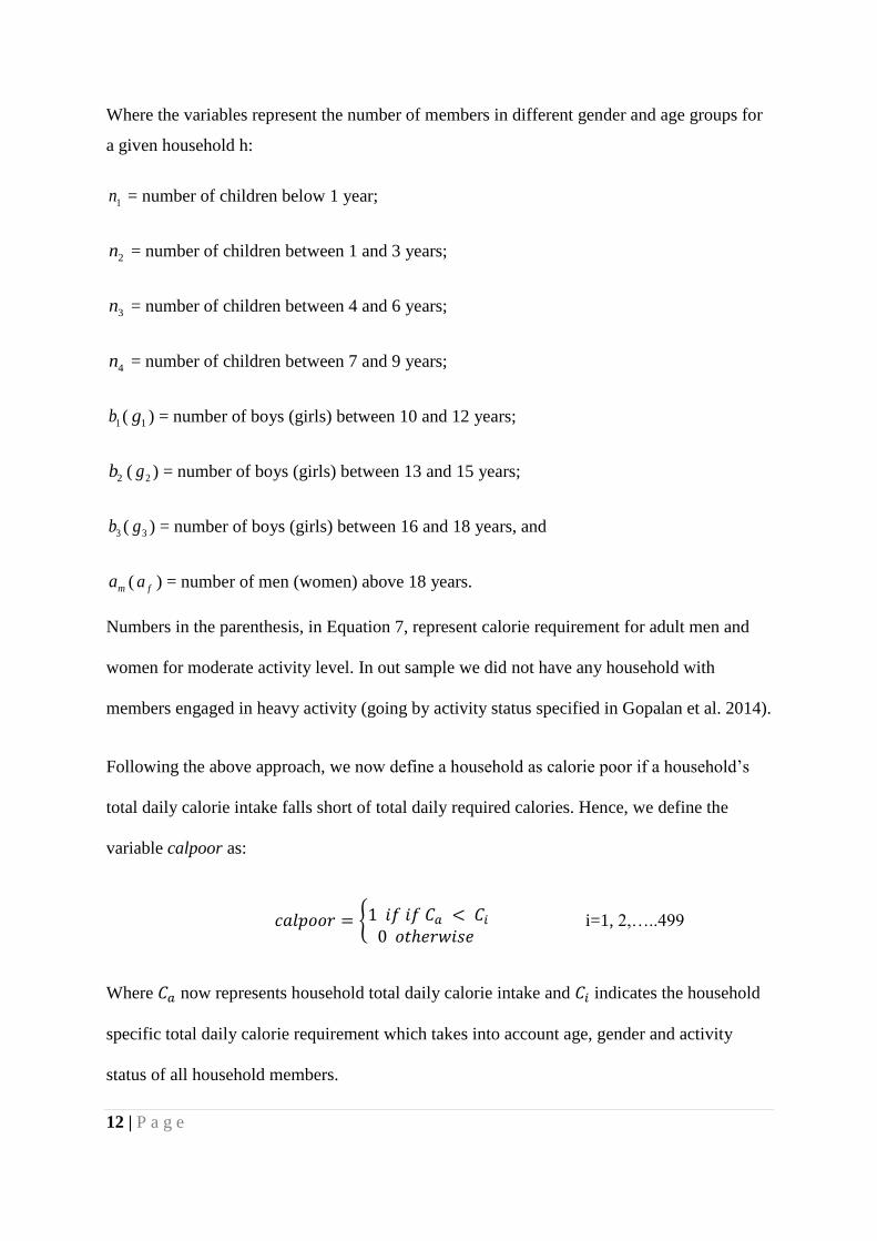
Following the above approach, we now define a household as calorie poor if a household’s
total daily calorie intake falls short of total daily required calories. Hence, we define the
variable calpoor as:
𝑐𝑎𝑙𝑝𝑜𝑜𝑟 = {
1 𝑖𝑓 𝑖𝑓 𝐶𝑎 < 𝐶𝑖
0 𝑜𝑡ℎ𝑒𝑟𝑤𝑖𝑠𝑒 i=1, 2,…..499
Where 𝐶𝑎 now represents household total daily calorie intake and 𝐶𝑖 indicates the household
specific total daily calorie requirement which takes into account age, gender and activity
status of all household members.

13 | P a g e
Income poverty. For the purpose of the present study, poverty line has been determined by
updating the poverty line for urban West Bengal, 2004, based on revised set of official
poverty lines specified by Tendulkar Committee (GOI 2011) which gives a poverty line
expenditure for 2010-11 of Rs.856.28 (see Maitra and Rao 2015 for further details).
Hence, variable poor is defined as:
𝑝𝑜𝑜𝑟 = { 1 Ya < Ymin
0 𝑜𝑡ℎ𝑒𝑟𝑤𝑖𝑠𝑒
Control Variables.
Apart from poverty, the other explanatory variables in the equation for calorie poverty
include household size (in logarithmic form); age, gender, education, homeownership status
and religion of household head; and household composition represented by the proportion of
children, working age adults and seniors in the household. The above variables are consistent
with the list of socio-economic indicators of food and nutrition security provided in Haddad,
et al. (1994) and Frankenberger (1992).
Additionally, we have three other variables in the income-poverty equation which are not
included in the equation for calorie poverty. These variables are: asset (= 1if no asset other
than fan, 0 otherwise) which describes household asset ownership status; hhtype (=1 if casual
labor household, 0 otherwise) which describes household employment status and lnfexp
which describes non-food expenditure in logarithmic form. The justification for inclusion of
these variables is explained in Section 3.3.1.

14 | P a g e
Table I reports summary statistics of the variables. About 61.72% of households in the
sample are calorie poor according to ICMR norm and 64.13% are calorie poor when we use
household specific calorie norm accounting for activity status, while 13% are income-poor.
About 19% of households in the sample have female headship and a large proportion (33%)
of households are headed by illiterate (or below primary) persons. Finally, 22% of
households in the studied sample are casual labor households, a sizable proportion, implying
concentration of employment in the informal sector. What we find most striking in this table
is that when disaggregated by calorie class and income class, the two groups of households
exhibit very different characteristics. Income poor households have larger family size, higher
share of female headed households and casual labor households, higher prevalence of
illiteracy and higher prevalence of asset poverty, among other characteristics.
[Table I here]
3.3 Statistical Analysis
First we examine whether the two groups of households exhibit any difference in terms of
pattern of consumption expenditure and food/nutrient consumption, through simple
descriptive statistics. For the purpose of the analysis in this section, we define the calorie
classes, with respect to the ICMR-prescribed calorie norm for urban India (fincal) — 2100
kcal per capita per day (ICMR 1988). These households will be termed as calorie poor for the
rest of the analysis in this section. The definition of income-poor stands as before.
Next, we present a cross tabulation of the calorie poor and income poor households to get a
preliminary idea on the relationship between the two variables – calpoor and poor, where

15 | P a g e
calorie poverty takes account of difference in activity status.9 Finally, we explore the
association between the two variables statistically through appropriate modelling techniques
– simultaneous probit estimation and BPSM for robustness. We also conduct sensitivity
analysis specifying different levels of poverty line expenditure for the cross tabulation and
empirical modelling mentioned above.
3.3.1 Empirical Model: Recursive Bivariate Probit Model
We attempt to model the calorie poverty and income poverty by the application of recursive
bivariate probit model. The theoretical exposition follows from Becker's household
production theory as discussed in Section 2.10 The model includes binary calorie poverty
status and poverty status as the joint dependent variables, with the latter appearing as an
ordinary pre-determined variable in the calorie poverty equation, along with households’
socio-economic and demographic characteristics. The fact that the binary endogenous
variable poverty status appears on the right hand side (RHS) only as observed, makes the
system recursive (Greene, 2012). That is, we want to identify the impact of actually being
9 We also checked cross tabulation with respect to fincal. Since the results are broadly similar
we report results for calpoor alone.
10 The bivariate probit model with an endogenous dummy belongs to the general class of
simultaneous equation models with continuous and discrete endogenous variables introduced
by Heckman (1978). In his systematic review of multivariate qualitative models Maddala
(1983) lists this model among the recursive models for dichotomous choice (Model 5).

16 | P a g e
poor on calorie poverty status of a household rather than the propensity of being poor
(Blundell and Smith, 1993).
The observed variables for a household’s calorie poverty status (𝑐𝑎𝑙𝑝𝑜𝑜𝑟𝑖) and income-
poverty status (𝑝𝑜𝑜𝑟𝑖) are related to the corresponding latent variables as 𝑐𝑎𝑙𝑝𝑜𝑜𝑟𝑖∗ and as,
𝑝𝑜𝑜𝑟𝑖∗
𝑐𝑎𝑙𝑝𝑜𝑜𝑟𝑖= {
0 1
𝑖𝑓 𝑐𝑎𝑙𝑝𝑜𝑜𝑟𝑖∗ ≥ 0
𝑖𝑓 𝑐𝑎𝑙𝑝𝑜𝑜𝑟𝑖∗ < 0
(8)
Where 0 indicates calorie sufficient and 1 indicate calorie-poor. And,
𝑝𝑜𝑜𝑟𝑖= {
0 1
𝑖𝑓 𝑝𝑜𝑜𝑟𝑖∗ ≥ 0
𝑖𝑓 𝑝𝑜𝑜𝑟𝑖∗ < 0
(9)
Where 0 indicates non-poor and 1 represents poor.
The underlying model consists of two separate equations relating the latent calorie poverty
status 𝑐𝑎𝑙𝑝𝑜𝑜𝑟𝑖∗ and income poverty status 𝑝𝑜𝑜𝑟𝑖
∗ to background characteristics of the
households, represented by vectors 𝑥1 and 𝑥2 respectively which include capital (human and
physical) and other exogenous variables, e.g. household socio-demographic characteristics.
𝑐𝑎𝑙𝑝𝑜𝑜𝑟𝑖∗ = �́�𝑝𝑜𝑜𝑟𝑖 + 𝑥1𝑖𝛽1𝑖 + 휀1𝑖
(10)
𝑝𝑜𝑜𝑟𝑖∗ = 𝑥2𝑖𝛽2𝑖 + 휀2𝑖
(11)
where 𝛽1 and 𝛽2 are column vectors of unknown parameters, �́� is the unknown scalar as
mentioned before, 휀1𝑖 and 휀2𝑖 are the error terms assumed to be distributed standard normal.
Our coefficient of interest in Equation 10 is γ ́. Full efficiency in estimation and an estimate

17 | P a g e
of γ ́ are achieved by full information maximum likelihood estimation, treating the above as a
bivariate probit model ignoring the simultaneity (Green 2012).11
But if calorie poverty and income poverty are jointly determined, estimating the probit
equation (Equation 10), as above, in isolation, will give a biased estimate of �́� (Greene,
2012). If the same set of unobserved characteristics influence both income poverty and the
likelihood of calorie poverty. This potential for unobserved heterogeneity will result in the
error term 휀1𝑖 in the above model being correlated with the explanatory variable(s) capturing
income poverty and if this is so, poor will not be exogenous.
The possible joint determination of 𝑦1𝑖 and 𝑦2𝑖 are accounted for by allowing the errors 휀1𝑖
and 휀2𝑖 to be distributed according to a standard bivariate normal distribution with correlation
as shown below:
𝐸(휀1𝑖) = 𝐸(휀2𝑖) = 0
𝑉𝑎𝑟(휀1𝑖) = 𝑉𝑎𝑟(휀2𝑖) = 1
𝐶𝑜𝑣(휀1𝑖,휀2𝑖) = 𝜌
The model allows us to conduct an endogeneity test to check the potential endogeneity of
𝑐𝑎𝑙𝑝𝑜𝑜𝑟 and 𝑝𝑜𝑜𝑟, by testing the significance of 𝜌. The single equation probit model
outlined in Equation 10 is a special case of the bivariate probit with 𝜌 = 0. Starting with the
latter model, the restriction 𝜌 = 0 is then tested. If 𝜌 is not significantly different from zero,
one concludes that the system is recursive and single equation probit estimation maybe
11 We can ignore the simultaneity in the model but not in the linear regression model because,
here, the log-likelihood is being maximised, whereas in the linear regression case certain
sample moments are being manipulated that do not converge to the population parameters in
the presence of simultaneity (Greene 2012).

18 | P a g e
suitable for the present purpose. In more general terms, the latter specification implies that
income-poverty is only exogenously influencing calorie poverty status of a household.
The bivariate probit’s coefficient estimates by themselves are of limited use when
interpreting the model results. Therefore, it is customary to report the marginal effects of the
explanatory variables on the probability of observing a certain outcome (see Appendix for
technical details).
Identification
The model was estimated by imposing an exclusion restriction even though it is not strictly
necessary as “identification by functional form” (normal distribution) is possible which only
requires variations in the set of exogenous regressors” (Wilde, 2000). However, we impose
exclusion restrictions to render estimation results more robust to distributional
misspecification (Monfardini and Radice 2006). The identifying variables in our model are
asset, hhtype and lnfexp - included only in vector x2 in the equation for poor (Equation 11)
and excluded from x1 in calpoor equation (Equation 10). Asset ownership reduces risk and
vulnerability in the long run enabling consumption smoothing, consistent with the idea of
sustainable livelihood approach in poverty reduction (Barett 2002; Bennett 2003). Hence
this variable is included in income-poverty equation, however, it is excluded from calorie-
poverty equation because ownership of assets is not likely to affect household calorie intake
in the short run. Regarding the variable hhtype, ‘casualization’ of labor is considered to be a
serious threat to poverty in the literature (Barrett 2002; Beneria and Floro 2006) and hence
included in the income-poverty equation. However, it is excluded from the calorie equation
because its effect on household calorie consumption will come through household poverty
status and as for the remaining effect which can permeate through activity status we’ve
19 | P a g e
already controlled for the latter in constructing the variable calpoor. Finally, we include the
variable lnfexp as an additional exclusion restriction because it has been used in the literature
as an instrument in estimating calorie-expenditure elasticity (Subramanian and Deaton, 1996;
Gibson and Rozelle 2002).
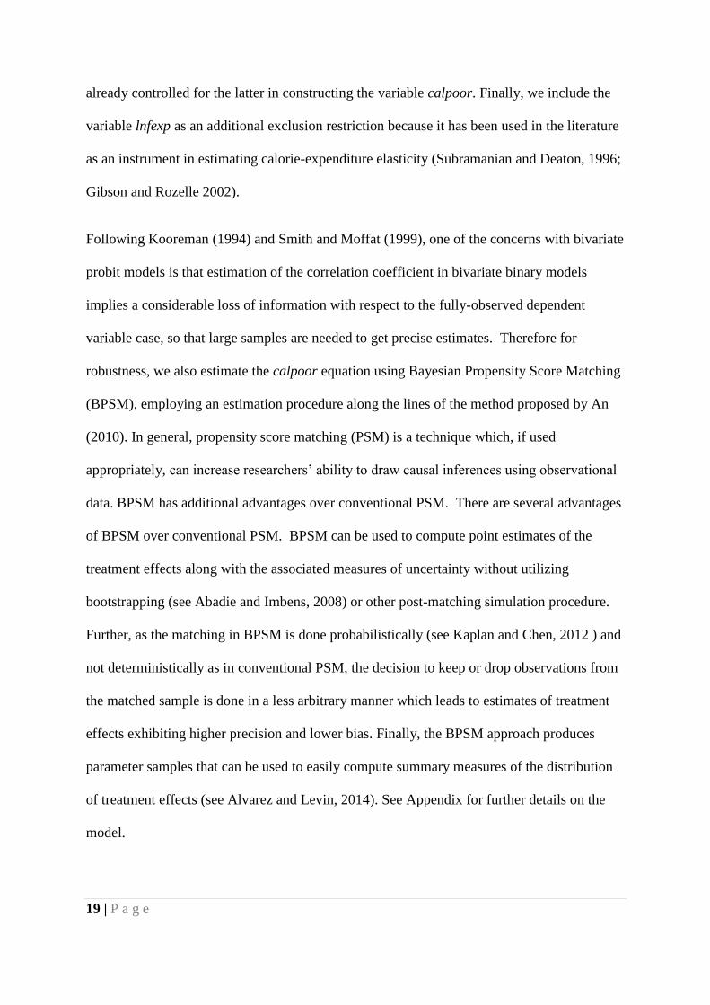
Following Kooreman (1994) and Smith and Moffat (1999), one of the concerns with bivariate
probit models is that estimation of the correlation coefficient in bivariate binary models
implies a considerable loss of information with respect to the fully-observed dependent
variable case, so that large samples are needed to get precise estimates. Therefore for
robustness, we also estimate the calpoor equation using Bayesian Propensity Score Matching
(BPSM), employing an estimation procedure along the lines of the method proposed by An
(2010). In general, propensity score matching (PSM) is a technique which, if used
appropriately, can increase researchers’ ability to draw causal inferences using observational
data. BPSM has additional advantages over conventional PSM. There are several advantages
of BPSM over conventional PSM. BPSM can be used to compute point estimates of the
treatment effects along with the associated measures of uncertainty without utilizing
bootstrapping (see Abadie and Imbens, 2008) or other post-matching simulation procedure.
Further, as the matching in BPSM is done probabilistically (see Kaplan and Chen, 2012 ) and
not deterministically as in conventional PSM, the decision to keep or drop observations from
the matched sample is done in a less arbitrary manner which leads to estimates of treatment
effects exhibiting higher precision and lower bias. Finally, the BPSM approach produces
parameter samples that can be used to easily compute summary measures of the distribution
of treatment effects (see Alvarez and Levin, 2014). See Appendix for further details on the
model.
20 | P a g e
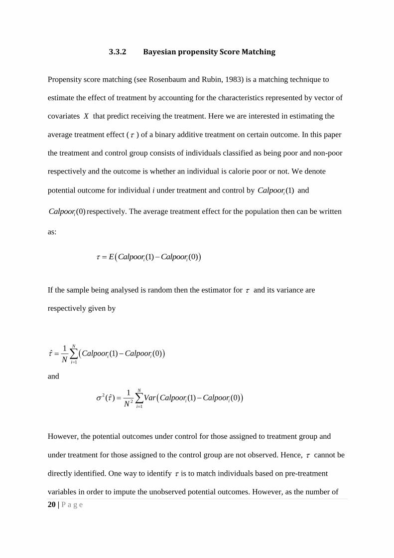
3.3.2 Bayesian propensity Score Matching
Propensity score matching (see Rosenbaum and Rubin, 1983) is a matching technique to
estimate the effect of treatment by accounting for the characteristics represented by vector of
covariates X that predict receiving the treatment. Here we are interested in estimating the
average treatment effect ( ) of a binary additive treatment on certain outcome. In this paper
the treatment and control group consists of individuals classified as being poor and non-poor
respectively and the outcome is whether an individual is calorie poor or not. We denote
potential outcome for individual i under treatment and control by (1)iCalpoor and
(0)iCalpoor respectively. The average treatment effect for the population then can be written
as:
(1) (0)i iE Calpoor Calpoor
If the sample being analysed is random then the estimator for and its variance are
respectively given by
1
1ˆ (1) (0)
N
i i
i
Calpoor CalpoorN
and
2
21
1ˆ( ) (1) (0)
N
i i
i
Var Calpoor CalpoorN
However, the potential outcomes under control for those assigned to treatment group and
under treatment for those assigned to the control group are not observed. Hence, cannot be
directly identified. One way to identify is to match individuals based on pre-treatment
variables in order to impute the unobserved potential outcomes. However, as the number of

21 | P a g e
pre-treatment variables increases, it becomes harder to match individuals. Rosenbaum and
Rubin (1983) proposed propensity score matching approach to overcome this issue. They
argued that matching individuals based on similar propensity scores is equivalent to matching
them based on the values of pre-treatment variables. Ignoring ties in propensity scores and
matching with replacement the PSM estimate of ATE can be written as
1
1ˆ (1) (0)
N
m i i
i
Calpoor CalpoorN
where (1)iCalpoor and (0)iCalpoor are calculated as follows:
{ }
1(0) (1 ) (0)
j ii i i i j rank p p L
j C
Calpoor D Calpoor D Calpoor IL
[12]
{ }
1(1) (1) (1 )
j ii i i i j rank p p L
j T
Calpoor D Calpoor D Calpoor IL
[13]]
In equations (12) and (13) above, L indicates the number of matches, C and T are sets
containing individuals in the control and treatment group respectively, iD is the treatment
dummy of ith individual and I is an indicator function which takes the value 1 if its argument
is true, otherwise it takes the value 0. In equations (12) and (13), jp are the predicted
propensity scores.
All models have been estimated in Stata (version 13).

22 | P a g e
4 Results
4.1 Consumption Expenditure and Dietary Pattern in Kolkata Slum Households: Disaggregated Analysis across calorie-poor and income-poor households, Kolkata, 2010-11
Table 2 presents percentage break-up of monthly total consumption expenditure in Kolkata
slum households over nine broad food groups and selected non-food items of consumption.
[Table 2 here]
Income-poor and calorie poor households spend more on cereals compared to any other food
group, however, the former group spends more on cereals compared to the latter who have
larger expenditure share on milk and milk products, fruits and meat-egg-fish. This pattern of
food expenditure roughly confirms the claim made by the literature that growing calorie
deficiency in India could be partly explained by dietary diversification away from calorie-rich
cereals to more expensive sources of calorie such as milk, fruits or meat (Pingali and Khwaja
2004). Miscellaneous food products seem to be having an important role in the consumption
expenditure of sampled households, with calorie poor households deriving relatively higher
share of calories from cakes, biscuits etc. and income poor households reporting large share
of calories from cooked meals.12 (Table 3) Interestingly, income poor households have higher
expenditure share of intoxicants13. Calorie-poor households have higher share of non-food
expenditure compared to income-poor households. They seem to be spending more on
medical, education and consumer durables compared to income-poor group.
13 Intoxicants include Country liquor, Beer etc.
23 | P a g e
[Table 3 here]
Looking at the nutrient-wise break-up of the food items consumed (Table 4), we find while
the average consumption of all three nutrients is inadequate for both groups of households,
average nutrient consumption is relatively more inadequate for income poor households.
With the exception of vegetables, similar pattern is observed for consumption of all food
items such as cereals, meat, fish and milk.
[Table 4 here]
We now look into a more detailed picture of consumption pattern of the households in terms
of nutrient share of each food item (Table 5).
[Table 5 here]
We note the following: while both groups of households are deriving maximum share of all
there nutrients from cereals, income poor households are obtaining a larger share of calories
from cereals followed by vegetables and miscellaneous food products compared to calorie
poor households. However, the latter are getting larger share of calories from pulses and
soyabean, milk and milk products, fruits and meat-egg-fish and edible oil compared to the
former. Similar pattern is noted for proteins and fat.
4.2 Cross-tabulation of Income Poor and Calorie Poor Households
Table 6 shows the joint distribution of poor and calpoor. Among the income-poor
households, 97% are also calorie poor. Interestingly, we note the presence of a large
proportion of the calorie poor households among the non-poor (60%).
[Table 6 here]
24 | P a g e
For further investigation, we conduct sensitivity analysis by defining alternative
specifications of the poverty line expenditure which include the following: a poverty line
which is less than 50% of the current cut-off of Rs. 856.28, one which is less than 25% of the
current cut-off, one which is 25% above the current poverty line and finally the one which is
50% above the current poverty line (Tables 7 and 8).
[Tables 7 and 8 here]
We find that the proportion of calorie poor households among the poor increases, as poverty
line expenditure is revised downward (from Rs. 856.28 to Rs. 642.28 to Rs. 428.14) (Table
7), and alternatively, the proportion decreases among the non-poor group of households as
poverty line is gradually revised upward from Rs. 428.14 to Rs. 1284.42) (Table 8).
Additionally, tetrachoric14 correlation between poor and calpoor is 0.68 which is also
statistically significant (Table 6). On the whole, the above analysis indicates that there exists
a strong direct association between poor and calpoor.
However, the most interesting aspect of these results is the presence of a large proportion of
calorie poor among the non-poor households no matter which poverty line we specify. Even
though the proportion decreases from 64% to 46% as we move across the lowest to the
highest poverty line expenditure, it remains fairly large across all non-poor samples,
14 If two ordinal variables are obtained by categorizing a normally distributed underlying
variable, and those two unobserved variables follow a bivariate normal distribution then the
(maximum likelihood) estimate of that correlation is the polychoric correlation. If each of the
ordinal variables has only two categories, then the correlation between the two variables is
referred to as tetrachoric (Greene and Hensher 2009).
25 | P a g e
declining to less than 50% only when we reach the upper limit of poverty line expenditure
(50% above original poverty line expenditure). It is this group of calorie poor households
among the non-poor that are of concern to the policy makers. Of equally great concern is the
fact that a higher concentration of calorie poor households (96%) is noted among the
transitioning non-poor households just above the poverty line (Rs.856.28 ≥ MPCE ≤ Rs.
1070.28).
To examine further what’s going on in the transitional households we undertake three further
investigations. First we examine the distribution of per capita daily calorie intake and MPCE
for the entire sample (in logarithmic form) (Figure 1) and find that calorie distribution is left-
skewed while expenditure distribution is slightly right skewed, generally giving the
impression that households with low level of expenditure may not also be consuming lower
calories at the same time. Calorie distribution also looks bimodal hinting at the presence of
two different distributions for different expenditure groups. Looking at calorie distribution
across poor, all non-poor and non-poor transitional households (Figure 2), we note that
bimodality originates from calorie distribution of non-poor households. We also note
considerable overlap in calorie distribution of all three groups with the largest overlap
occurring for poor and transitional households.
[Figure 1 and Figure 2 here]
Next we conduct a preliminary investigation into the shape of the calorie-expenditure
function through non-parametric regression which estimates the function m (x = E (y|x), by
computing an estimate of the location of 𝑦 within a specific band of 𝑥, where in our case 𝑦=
logarithm of per capita daily calorie intake and 𝑥=logarithm of MPCE. We estimate 𝑚(𝑥)
using Locally Weighted Regression Smoothing (Lowess). The Lowess plot (Panel A, Figure

26 | P a g e
3) exhibits non-linearity in calorie-expenditure relationship for the entire sample. The slope
of the calorie-expenditure plot rises till a certain level of expenditure after which it becomes
flat – signifying increased response of calorie demand to rise in the level of expenditure till a
certain expenditure level after which it declines. However, for the transitional households
(panel C, Figure 3) we note a decline in calorie response to increased expenditure at first, a
slight rise in slope (roughly at log 6.84) afterwards and then quite a sharp decline somewhere
between MPCE Rs. 998.25 and Rs. 1096 (log 6.907 and log 7) before it rises again.
Comparing the above with calorie response of poor households in Panel B of Figure 3, we
find the slope rises steeply at first but declines after reaching an expenditure level of log 6.75
roughly.
[Figure 3 here]
Motivated by the above results, we now estimate calorie expenditure elasticity across all
expenditure classes by regressing per capita adjusted household calorie intake on MPCE
controlling for household socio-demographic characteristics (see Appendix for details). Two
major observations follow: First, calorie expenditure elasticity is positive and significant but
non-linear, declining progressively as poverty line expenditure is upwardly revised. Second,
for the transitional households calorie expenditure elasticity is positive but not significant.
Interestingly, it is also insignificant for households just below poverty line.
It is this lack of one-to-one correspondence between income-poor and calorie-poor
households which now motivate us to turn to the results of the empirical models where we
control for other predictors of calorie poverty while taking account of endogeneity of income
poverty and calorie poverty.

27 | P a g e
4.3 Recursive Bivariate Probit Model
We present results for both specifications of calorie intake and all specifications of poverty
line expenditure (Tables 9). However, for poverty line expenditure set at 25% below poverty
line we could not estimate recursive bivariate probit model, even though results are available
for BPSM. The results from recursive bivariate probit model indicate that marginal effect of
income poverty is positive and significant at 5% level of significance (Table 9) - the
(conditional) probability of being calorie poor being 0.59 higher for income poor households
relative to non-poor households. However, parameter ρ which represents the correlation
between the error terms in the two equations is not significantly different from zero,
suggesting that the system is recursive and standard probit may be suitable for the present
purpose. Results from both sets of models are broadly similar.15 It is only when poverty line
expenditure is set at 50% above poverty line expenditure that ρ is significant at 10% level of
significance.
[Table 9 here]
Interestingly, when poverty line expenditure is set at 25% above current poverty line the
marginal effect of income poverty on calorie poverty is positive but insignificant. However, it
is positive and significant again for all other specifications of poverty line expenditures
(Table 9).
Results of BPSM indicate similar pattern (Table 10). For calpoor and poor, results indicate
poor households have 0.38 higher probability of experiencing calorie poverty compared to
non-poor households. Sensitivity analysis with various other poverty line expenditures
15 Probit results are not reported here but are available upon request.

28 | P a g e
indicate similar pattern except when poverty line is set at 25% above poverty line, for which
the effect of income poverty on calorie poverty is significant unlike in the bivariate probit
model.
[Table 10]
5 Discussion
Results indicate that the probability of a household being income poor increases the chances
that it will be calorie poor as well, controlling for other predictors of calorie poverty. Our
finding supports the notion that being poor would imply being deprived of full nutritional
capabilities (Osmani 1992). One reason why a poor household is likely to be more calorie
deprived is relatively straightforward and refers to affordability. Especially so because urban
poor are net buyers of food (FAO 2008). Furthermore, eating healthy could be expensive
(Wiggins et al. 2015), more so with recent rise in in food prices in India and elsewhere
(Anand et al. 2016). Over the past decade, India has seen a prolonged period of persistently-
high food inflation and one of the major contributors to food inflation has been cereals
closely following milk and egg-meat-fish (Bhattacharya and Sengupta 2015). This finding is
also somewhat driven by certain observations from Table 1 such as: income poor households
have higher proportion of female headed households and casual labour households and they
report higher prevalence of illiteracy. The nutrition literature has adequate evidence that such
households will be at greater risk of calorie deprivation (Floro and Swain 2013; Benson
2007).
However, the only case when the finding is not robust is when poverty line expenditure is set
at 25% above the poverty line. For this specification, the marginal effect of income on calorie
poverty becomes insignificant for the simultaneous probit model. Detailed investigation of
29 | P a g e
calorie behaviours of households show that the majority of transitional households (856.28
≤MPCE≤ 1070.35) just above the poverty line expenditure are calorie poor and for them
calorie-expenditure elasticity is not significant. The lowess plot shows somewhat erratic
movement with elasticity dropping sharply at per capita expenditure level of roughly Rs.992.
The above findings indicate that the interaction between income poverty and calorie poverty
is not very straightforward. The findings almost echo Lipton (1983) who argues at very low
levels of expenditure, calorie intake rises slowly with increase in income and may even fall
because households wary of the monotony of their diet spend the extra outlay on more
expensive calories which they had wanted to consume but could not afford to because of
income constraint. Behrman et al. (1988) also contend in similar lines that some desire for
food variety is suppressed in order to subsist at very low level of income but once that level is
crossed taste may get preference. Banerjee and Duflo (2007) also contend that when income
increases for the poor household they may demonstrate greater preference for taste as
opposed to more nutritious food.
Another interesting result is ρ being positive and significant at 10% level when poverty line
expenditure is set at a higher level (50% above poverty line) implying that at higher level of
expenditure, same set of unobserved factors which influence the probability of a household
becoming income poor (such as a policy change in the economy resulting in changing health
care plan and increased out-of-pocket expenditure) might also raise the probability of being
calorie poor. However, for lower level of poverty line expenditure the unobserved
heterogeneity influencing the probability of being calorie poor is not significantly associated
with the unobserved influences on the likelihood of being income poor.
Notwithstanding the fact that we find positive association between risk of income poverty
and calorie poverty, we note a lack of one-to-one correspondence between calorie poverty

30 | P a g e
and income poverty. A large proportion of calorie poor households is found to be nested
within non-poor households. In fact, non-poor households have higher share of calorie poor
as opposed to calorie sufficient households. This result is striking and it indicates that calorie
shortfall is not a result of income deprivation alone. It is possible that part of the incidence of
calorie poverty is the outcome of deliberate choice (Banerjee and Dufflo 2011b), or is driven
by less backbreaking work, or occurring due to dietary diversification (Pingali and Khwaja
2004) which indicates a possibility that calorie might become an inferior good at some point
in time. What forces are driving these shifts in dietary pattern is beyond the scope of the
present paper. However, what is relevant for the present study is the fact that the findings are
based on urban low income households which are characterized by higher participation of
women in labor force and of working parents whereby work–family spillover is likely to
affect food choice often leading to lower quality food (Devine et al. 2006). Another driver of
low calorie consumption in the context of the urban sample could be greater scope for
demonstration effect to be in action driven by a more diversified food basket, and could
explain some of the reasons for an increase in the cost of calories consumed by the urban
poor (Vepa 2004).
Placing the findings in broader context, India is not the only country where we observe such
peculiar result. Another case in point is China, a transitional economy where the total energy
intake was decreasing among all income groups (Du et al. 2004) between 1985 and 1997. The
structure of the Chinese diet was changing with improved income, particularly in the low-
and middle income groups, where people in the low-income group have the highest decrease
in cereal food intakes. A possible explanation for both cases – India and China- could be the
much discussed non-linearity of calorie-expenditure elasticity (Strauss and Thomas 1990;
Roy 2001; Gibson and Rozelle 2002) that exists in our sample too — responsiveness of

31 | P a g e
calorie demand to expenditure decreases due to rise in the level of expenditure due to
households switching away from calorie-rich cheap cereals to more expensive sources of
calorie, thus demonstrating a preference for quality. May be at this level of expenditure, non-
food items like education and health care also start competing with food items, for a larger
share of the extra outlay, leading to an actual fall in calorie intake. This could explain why
cross tabulation of both groups of households shows, even if proportion of calorie poor is
declining as poverty line expenditure moves up, the fraction of calorie poor households
among the non-poor remains fairly large — more than 50% in most cases.
Our analysis of expenditure and dietary pattern of the urban slum households corroborate the
above. Overall findings from this analysis indicate that expenditure pattern of calorie-poor
group might be dominated by the spending behaviour of non-poor households. The
expenditure and dietary pattern of poor and calorie poor households are similar in many
respects. However, the calorie poor households do exhibit consumption patterns expected to
be noted with respect to non-poor households on certain occasions, clearly bringing out the
fact that there are several non-poor households among the calorie poor.
Comparing our results with those from the previous literature, the evidence that exist in India
is mostly based on bivariate specifications of calorie shortfall and income poverty. For
example, Meenakhshi and Viswanathan (2003) note apparent lack of correlation between
income and calorie deprivation. Suryanarayan and D'silva (2007) found positive and
significant association between incidence of poverty and different measures of per capita
calorie deprivation at the regional level for both rural and urban India. As for studies outside
India, Rose et al. (1999) estimated the relationship between income poverty and food
insufficiency defined in terms of calorie deficiency in the context of US economy using panel
data by estimating a multivariate logit model and found that those in poverty were over 3.5
32 | P a g e
times more likely to be food insufficient. Interestingly, they too report that a one-to-one
correspondence between poverty-level incomes and food insufficiency does not exist — half
of those experiencing food insufficiency had incomes above the poverty level. Since our
results echo similar findings in an entirely different context – low income urban households
from an emerging economy – it indicates it is high time we revisit the nutrition-poverty
linkage and explore what’s actually going on using panel data and larger samples.
At this stage it may be useful to identify some limitations of the present research. First, as
mentioned above, we have used cross section data while a panel data would have provided
better insight on our hypothesis. Given the fact that our study sample is low income urban
slum households in Kolkata, to what extent the results can be generalized in the context of the
broader setting of urban India also remains a question. Given the scope of the present
analysis, we identify these issues for future research. Future research should also consider
exploring the issue in the context of a rural sample.
6 Conclusion
In the light of the apparent contradiction between trends in calorie poverty and income
poverty, noted in the Indian households over the past few decades, this paper seeks to
examine whether there’s any direct association between calorie poverty and income poverty
in cross section data, based on a random sample of 500 households in slums of Kolkata in
2010-11. The hypothesis tested is: income poor and calorie poor households may not be the
same. Calorie deprivation is estimated using household specific calorie norm which takes
account of age, gender and activity status of each household member in deciding on the
household level cut-off. The association between income poverty and calorie poverty is

33 | P a g e
tested using modelling techniques which account for endogeneity in the relationship between
the two variables. Additionally, BPSM is used to ensure robustness.
Results indicate that an income poor household is more likely to be calorie poor. However,
there is no one-to-one correspondence between calorie poverty and income poverty to the
extent we find a large number of calorie poor households among the non-poor. The policy
implications of the above findings are manyfold. First, targeting income poor households for
subsidy – in cash or in kind - should address calorie poverty as well. In general, anti-poverty
policies should be successful in addressing calorie deprivation. Public policy can also
formulate provisions for minimum cost of healthy diet for the poor households. Second,
income poor rather than calorie poor households should be targeted for cash/food subsidies
since household calorie behavior might be influenced by factors not related to resource
constraint. Many countries use food price subsidies to encourage greater nutrition. However,
subsidizing food such as cereals would not have any effect on calorie consumption if
households consume less cereal and more shrimps, where shrimps are not very nutritious per
dollar spent (Banerjee and Dufflo 2011a). Finally, separate nutrition policy is desirable for
transitional households just above the poverty line. Providing income subsidy to poor
households to push them just above poverty line is not going to be much beneficial in terms
of calorie gain because these households have very different calorie behaviour where taste
may get preference over calories when income increases. So what might be necessary in this
case, to achieve meaningful nutrition related gain, may be a ‘big push’ which might place the
household substantially above poverty line. One policy recommendation pertinent to both
groups of households is nutrition education. For the poor households it would imply learning
to balance low wages and healthy eating and for the non-poor households it would imply
learning the values of good nutrition.

34 | P a g e
Apart from nutrition related policies there are also health implications of the results. As (Du
et al. 2004) argues, increased income might have affected diets and body composition in a
detrimental manner to health, with those in low-income groups having the largest increase in
detrimental effects due to increased income. On one hand, as long as declining calorie is
compensated by other nutrients, more specifically, increased consumption of micronutrients;
it may be less of a concern. On the other hand, even if other nutrients are consumed in
increased quantity sufficient calorie intake might be necessary to ensure proper absorption of
those other nutrients by the body (Vepa 2004). It is also possible that current nutrient intake
may not have significant impact on health indicators (Behrman et al.1988) because “within
limits, human metabolism adjusts in response to nutrient intakes, with little impact on health
indicators” (Sukhatme 1982 and Payne 1987; cited in Behrman et al. 1988, page 302).
Additionally, large intrapersonal variation in nutrient intakes over time make current nutrition
intakes very poor proxies for the medium- or longer-run nutrient intakes of relevance for the
health indicators used (Sukhatme 1982; Srinivasan 1981; cited in Behrman et al. 1988). In
which direction Indian households are going is not very clear at this stage and requires a
detailed analysis of changes in nutrient consumption undergoing in these households. Such
exercises would be worth considering for future research.
In understanding the poverty-nutrition linkage we must not also forget that it is not just the
story of reduced poverty promoting better nutrition, but at the same time it is also possible
that better nutrition promotes better productivity and longer and healthy life (Dasgupta 1993).
“Better-nourished individuals constitute the bedrock of a nation that respects human rights
and strives for high labor productivity. Well-nourished mothers are more likely to give birth
to well-nourished children who will attend school earlier, learn more, postpone dropping out ,
marry and have children later, give birth to fewer and healthier babies, earn more in their
35 | P a g e
jobs, manage risk better, and be less likely to fall prey to diet-related chronic diseases in
midlife” (Haddad 2002, page 3). Therefore for policy makers, establishing the correct link
between nutrition and poverty is a necessity in tackling the triple curses of poverty-hunger-ill
health.
36 | P a g e
7 References
1. Abadie, Alberto and Guido W. Imbens, “On the Failure of the Bootstrap for Matching
Estimators”, Econometrica 76:6(2008), 1537-57.
2. An, Weihua, “Bayesian Propensity Score Estimators: Incorporating Uncertainties in
Propensity Scores into Causal Inference”, Sociological Methodology 40: 1(2010),
151-189.
3. Anand, R., Kumar, N. and Volodymyr, Tulin, “Understanding India’s Food
Inflation: The Role of Demand and Supply Factors,” IMF Working Paper No.
WP/16/2 (2016).
4. Alvarez, R. M. and Levin, I, “Uncertain neighbors: Bayesian propensity score
matching for causal inference,” Working Paper (2014). Available at:
https://polisci.wustl.edu/files/polisci/imce/slammlevin.pdf.
5. Banerjee, Abhijit and Duflo, Esther, “More than 1 Billion People are Hungry in the
World. But what if the Experts are Wrong? ” Foreign Policy, May/June (2011b).
6. Banerjee, Abhijit and Duflo, Esther, “Lecture 5: Is there a Nutrition Based Poverty
Trap? 14.73 Challenges of World Poverty (2011a). Available at:
http://ocw.mit.edu/courses/economics/14-73-the-challenge-of-world-poverty-spring-
2011/lecture-notes/MIT14_73S11_Lec5_slides.pdf.
7. Banerjee, Abhijit and Duflo, Esther, “The Economic Lives of the Poor”, Journal of
Economic Perspectives,” 21:1(2007), pp.141-167.
8. Barrett, Christopher B., 2002. "Food Security and Food Assistance Programs," in: B.
L. Gardner & G. C. Rausser (Eds.), Handbook of Agricultural Economics, edition 1,
volume 2, chapter 40, pages 2103-2190 (Elsevier 2002).

37 | P a g e
9. Basu, D. and A. Basole, “The Calorie Consumption Puzzle in India: An Empirical
Investigation,” PERI Working Paper Series No.285 (2012), Political Economy
Research Institute, University of Masachsetts Amherst.
10. Becker, G, "A Theory of the Allocation of Time," Economic Journal, 75: 299 (1965):
493-517.
11. Behrman, J. R. and A. Deolalikar, "Will Developing Country Nutrition Improve with
Income? A Case Study of Rural South India," Journal of Political Economy, 95(31)
(1987): 492-507.
12. Behrman, J., Deolalikar, A. and Wolfe, B, “Nutrients: Impacts and Determinants,”
The World Bank Economic Review 2:3 (1988), 299-320.
13. Beneria, Lourdes and Maria Floro, “Labor Market Informalization, Gender and
Social Protection: Reflections on Poor Urban Households in Bolivia and Ecuador,” in
S. Razavi and S. Hassim (Eds), Gender and Social Policy in a Global Context,
Palgrave Macmillan (2006), pp. 193-217.
14. Bennett, Lynn, “Using Empowerment and Social Inclusion for Pro-Poor Growth: A
Theory of Social Change,” Working Draft of Background Paper for Social
Development Strategy Paper (2002), Washington, DC: World Bank.
15. Benson, T. “Study of Household Food Security in Urban Slum Areas of Bangladesh”,
Final Report for World Food Programme (2007), International Food Policy Research
Institute, Food Consumption and Nutrition Division, IFPRI, Washington.
16. Bhattacharya, R. & Sen Gupta, A, “Food Inflation in India: Causes and
Consequences” Working Paper No. 2015-151(2015), National Institute of Public
Finance and Policy. New Delhi. Available at: www.nipfp.org.in.

38 | P a g e
17. Bouis, H. E. and L. Haddad, "Are Estimates of Calorie-income Elasticity too High? A
Recalibration of the Plausible Range," Journal of Development Economics,
39:2(1992): 333-364.
18. Chandrasekhar, C.P. and J. Ghosh, “The Calorie Consumption Puzzle”, Hindu
Business Line (11 February 2003).
19. Dasgupta, P, “An Inquiry into well-being and Destitution,” (Oxford: Oxford
University Press 1993).
20. Deaton, A. and Drèze, J.P., “Food and Nutrition in India: Facts and Interpretations,”
Eonomic and Political Weekly, 14 February, XLIV.7 (2009). Available at:
http://www.princeton.edu/~deaton/downloads/Food_and_Nutrition_in_India_Facts_a
nd_Interpretations.pdf.
21. Devine, C. M., Jastran, M., Jabs, J. A., Wethington, E., Farrell, T. J. and Bisogni, C.
A., “A lot of sacrifices: Work-family spillover and the food choice coping strategies
of low wage employed parents,” Social Science & Medicine 63:10 (2006), 2591–
2603. http://doi.org/10.1016/j.socscimed.2006.06.029.
22. Du, Shufa, Mroz, Tom A, Zhai, Fengying, Popkin and Barry M., “Rapid income
growth adversely affects diet quality in China—particularly for the poor!” Social
Science & Medicine, Vol.59:7) (2004), pp.1505-1515.
23. Floro, M. S. and R. Bali Swain, “Food Security, Gender, and Occupational Choice
among Urban Low-Income Households, “ World Development, 42:0(2013): 89-99.
doi:10.1016/j.worlddev.2012.08.005.
24. Food and Agricultural Organization (FAO), “State of Food Insecurity in the World,”
Rome, Italy. Food and Agricultural Organization of the United Nations (2008).
25. Frankenberger, T, “Indicators and Data Collection Methods for Assessing Household
Food Security,” in S. Maxwell and T. Frankenberger (Eds.), Household Food

39 | P a g e
Security: Concepts, Indicators, Measurements: A Technical Review, New York and
Rome, UNICEF and IFAD.
26. Gaiha, R., R. Jha and V. S. Kulkarni, “Prices, Expenditure and Nutrition in India”,
Working Paper No.2010/15 (2010), Australia South Asia Research Centre, Australian
National University.
27. Garrett, J. L. and M. T. Ruel, "Are Determinants of Rural and Urban Food Security
and Nutritional Status Different? Some Insights from Mozambique,” World
Development, 27:11(1999), 1955-1975.
28. Gibson, J. and S. Rozelle, "How Elastic is Calorie Demand? Parametric,
Nonparametric, and Semiparametric Results for Urban Papua New Guinea, " Journal
of Development Studies, 38:6 (2002): 23-46.
29. Gopalan, C., Sastri, B. V. R and S. C. Balasubramanian, “Nutritive Values of Indian
Foods”, Hyderabad, Indian Council of Medical Research (1991), National Institute of
Nutrition.
30. Government of India (GOI), “ Press Notes on Poverty Estimates”, New Delhi,
Planning Commission (2011).
31. Greene, W. (2003). Econometric Analysis. Prentice Hall.
32. Greene, W., Econometric Analysis, New Jersey, USA, (Prentice Hall PTR, 2012).
33. Greene, W. H. and D. A. Hensher, Modelling Ordered Choices, Mimeo, New York,
Stern School of Business (2009).
34. Haddad, L., Kennedy, E. and Sullivan, J., "Choice of Indicators for Food Security and
Nutrition Monitoring," Food Policy 19:3(1994): 329-343.
35. Haddad, L., “Nutrition and Poverty,” in Nutrition: A Foundation for Development,
Geneva: ACC/SCN (2002). Available at:
http://www.fao.org/docrep/011/i0291e/i0291e00.htm.

40 | P a g e
36. Indian Council of Medical Research (ICMR), “Recommended Daily Allowances of
Nutrients and Balanced Diets,” Nutritional Expert Group, Hyderabad: National
Institute of Nutrition (1988).
37. Lancaster, K. J, "A New Approach to Consumer Theory," Journal of Political
Economy, 74 (1966), 132-157.
38. Li, N. and S. Eli, “In Search of India’s Missing Calories: Energy Requirements and
Calorie Consumption,” Available for download at:
http://emlab.berkeley.edu/webfac/emiguel/e271 f10/Li.pdf (2010).
39. Lipton, M, “Poverty, Undernutrition, and Hunger”, Washigton, D.C, World Bank
Staff Working Papers No. 597 (1983), The World Bank.
40. Lohr, L. S, “Sampling: Design and Analysis,” Duxbury Press: An Imprint of
Brooks/Coles Publishing Company (1999), A Division of An International Thomson
Publishing Company.
41. Maddala, G. S, “Limited-Dependent and Qualitative Variables in Econometrics”,
Cambridge, Cambridge University Press (1983).
42. Maitra , C, “Measurement and Analysis of Food Security: A case of Urban India”,
The University of Queensland, Brisbane, Australia, (Unpublished doctoral thesis)
(2013).
43. Maitra, C. & Rao, D.S.P, "Poverty–Food Security Nexus: Evidence from a Survey of
Urban Slum Dwellers in Kolkata, " World Development, vol. 72 (2015), pp. 308-325.
doi:10.1016/j.worlddev.2015.03.006.
44. Maxwell, D, 1999, “The political economy of urban food security in sub-Saharan
Africa”, World Development, 27:11(1999), 1939-1953. doi:10.1016/S0305-
750X(99)00101-1.

41 | P a g e
45. Mehta , J. and S. Venkatraman , "Poverty Statistics: Bermicide’s Feast, " Economic
and Political Weekly, 35(27) (2000): 2377-2382.
46. Meenakshi, J. V. and B. Vishwanathan, “Calorie Deprivation in Rural India, 1983-
1999/2000," Economic and Political Weekly, 38:4 (2003): 369-375.
47. Monfardini, C. and R. Radice, “Testing Exogeneity in the Bivariate Probit Model: A
Monte Carlo study,” Italy, Department of Economics, University of Bologna (2006).
48. M.S. Swaminathan Research Foundation (MSSRF), “Food Insecurity Atlas of Urban
India,” Chennai, M.S. Swaminathan Research Foundation and the World Food
Programme (2002).
49. National Sample Survey Organisation (NSSO), Urban Frame Survey. Kolkata,
National Sample Survey Organisation (2008).
50. National Sample Survey Organisation (NSSO), Nutritional Intake in India (Report
No. 513, 61ST Round, July 2004 - June 2005). New Delhi: National Sample Survey
Organisation (2007), Ministry of Statistics & Programme Implementation,
Government of India.
51. Osmani, S. R, “Introduction,” in S. R. Osmani (ed.), Nutrition and Poverty. New
York: Oxford University Press for UNU-WIDER (1992).
52. Richard Palmer-Jones, and Sen Kunal. "On India's Poverty Puzzles and Statistics of
Poverty." Economic and Political Weekly 36.3 (2001): 211-17.
53. Patnaik, Utsa, “On Some Fatal Fallacies, ” Economic and Political Weekly, 20 Nov,
XLV.47 (2010).
54. Payne, Philip, "Public Health and Functional Consequences of Seasonal Hunger and
Malnutrition," in David E. Sahn (ed.), Causes and Implications of Seasonal
Variability in Household Food Security, Washington, D.C.: International Food Policy
Research Institute (1987).

42 | P a g e
55. Pingali, Prabhu and Khwaja, Yasmeen, “Globalization of Indian Diets and the
Transformation of Food Supply Systems, “ESA Working Paper 04–05 (2004), Rome:
Agricultural and Development Economics Division. Food and Agricultural
Organization of the United Nations.
56. Radhakrishna, R, "Food and Nutrition Security of the Poor: Emerging Perspectives
and Policy Issues,” Economic and Political Weekly, 40: 18 (2005): 1817-1823.
57. Rao, C. H. Hanumanthu, “Declining Demand for Food grains in Rural India: Causes
and Implications, ” Economic and Political Weekly 35.4 (2000): 201–6.
58. Ray, R. and G. Lancaster, “On Setting the Poverty Line Based on Estimated Nutrient
Prices: Condition of Socially Disadvantaged Groups during the Reform Period,"
Economic and Political Weekly, 40:1 (2005): 46-56.
59. Rose, D., Victor Oliveira and C. Gundersen, “Socio-Economic Determinants of Food
Insecurity in the United States: Evidence from the SIPP and CSFII Datasets, ” Food
and Rural Economics Division, Economic Research Service, U.S. Department of
Agriculture, Technical Bulletin No. 1869 (1998).
60. Rose, D, “Economic Determinants and Dietary Consequences of Food Insecurity in
the United States,” The Journal of Nutrition, 129: 2 (1999), 517.
61. Roy, N. (2001). "A Semiparametric Analysis of Calorie Response to Income Change
across Income Groups and Gender." Journal of International Trade and Economic
Development, 10:1 (2001): 93-109.
62. Ruel, M., Garrett, J., Morris, S., Maxwell, D., Oshaug, A., Engle, P., Menon, P.,
Slack, A. and Haddad, L, “Urban challenges to food and nutrition security: A review
of food security, health, and caregiving in the cities,” Food Consumption and
Nutrition Division Discussion Paper No. 51(1998), Washington, DC, International
Food Policy Research Institute.

43 | P a g e
63. Sen, A. K, “Social Exclusion: A Critical Assessment of the Concept and its
Relevance,” Paper Presented at the Asian Development Bank (1998).
64. Sen, P, "Of Calories and Things: Reflection on Nutritional Norms, Poverty Lines and
Consumption Behaviour in India,” Economic and Political Weekly, 40: 43 (2005):
4611-4618.
65. Smith, Lisa C, “The Great Indian Calorie Debate: Explaining Rising
Undernourishment during India's Rapid Economic Growth,” IDS Working Papers,
Vol.2013: 430(2013), pp.1-35.
66. Srinivasan, T. N, "Malnutrition: Some Measurement and Policy Issues, "Journal of
Development Economics, 8 (1981), 3-19.
67. Strauss, J. and D. Thomas, “The Shape of the Calorie Expenditure Curve,” Economic
Growth Centre Discussion Paper No. 595 (1990), Yale University.
68. Subramanian, S. and A. Deaton, "The Demand for Food and Calories," Journal of
Political Economy, 104(1) (1996), 133-162.
69. Sukhatme, P. V., ed. 1982. Newer Concepts in Nutrition and Their Implications for
Policy. Pune, India: Maharashtra Association for the Cultivation of Science Research
Institute.
70. Suryanarayan, M. H. and D Silva, "Is targeting the Poor a Penalty on the Food
Insecure? Poverty and food Insecurity in India," Journal of Human Development, 8:1
(2007): 89-107.
71. United Nations (UN), “The Millennium Development Goals Report: 2006”, United
Nations Development Programme (2006),
www.undp.org/publications/MDGReport2006.pdf.

44 | P a g e
72. Vepa, S. S, “Impact of globalisation on food consumption of urban India. in: FAO
Technical Workshop on Globalization of Food Systems: Impacts on Food Security
and Nutrition. 8–10 October 2003, Rome, Italy (2004).
73. Viswanathan, B. and J.V. Meenakhshi, “Changing Pattern of Undernutrition in India:
A Comparative Analysis Across Regions, “ Research Paper No.2006/118 (2006),
UNU-WIDER.
74. Wiggins, S., Keats, S., Han, E., Shimokawa, S., Alberto, J., Hernández, V. & Claro,
R.M, The rising cost of a healthy diet: changing relative prices of foods in high-
income and emerging economies,” London, Overseas Development Institute 2015).
Available at: https://www.odi.org/rising-cost-healthy-diet.
75. Wilde, J, “Identification of multiple equation probit models with endogenous dummy
regressors, ” Economic Letters, 69 (2000), 309-12.

45 | P a g e
76.
Table 1: Summary Statistics of Variables, IV-Oprobit Model, Kolkata, 2010-11.
Variables Definition Mean
All calorie poor income poor
calpoora household is calorie poor 64.13 - -
fincalb household is calorie poor 61.72 - -
poorc household is poor 0.13 - -
lnhhsize Logarithm of household size 1.37 (0.54) 1.53 (0.43) 1.68 (0.44)
hage Age of household head (years) 47.86 (13.77) 47.19 (14.24) 44.92 (14.07)
genderh =1 if female, else 0 0.19 0.19 0.27
dwelling =1 if owns home else 0 (hired or encroached) 0.33 0.36 0.39
relig0 Omitted base group household belongs to Hinduism 0.52 0.51 0.50
relig1 Equals 1 if household belongs to Islam, else 0 0.44 0.45 0.48
relig2 Equals 1 if household belongs to ’Christianity or Others’ else 0 0.04 0.04 0.02
headlit0 Omitted base group household head lliterate/ below primary
level education
0.33 0.36 0.64
headlit1 =1 if household head has primary to middle level education, 0
otherwise
0.58 0.57 0.35
headlit2 =1 if household head is graduate and above, 0 otherwise 0.09 0.07 0.02
kids Omitted base group share of kids (1-14 years) in the HH 0.18 (0.20) 0.24 (0.21) 0.31 (0.21)
workadult Share of working age adults (15-64 years) in the households 0.75 (0.23) 0.70 (0.22) 0.64 (.19)
senior Share of seniors aged 65 years and above 0.07(0.16) 0.06 (0.15) 0.05 (0.11)
assetd =1 if no durable asset or only fan, 0 otherwise .13 0.14 0.29
hhtypee =1 if casual labor household, else 0 0.22 0.25 0.42
lnnfexp Logarithm of non-food expenditure 7.73 (0.65) 7.71 (0.54) 7.29 (0.50)
Notes: Total number of households: 499.Standard Errors in parenthesis reported for continuous variables only. aHousehold is calorie poor
if total daily calorie intake is less than household specific total daily calorie requirement adjusted for age, gender and activity status of
each family member. b If per capita daily calorie intake < 2100 kcal per capita per day (ICMR 1988). cPoverty line expenditure for
Kolkata, 2010-11, was determined by updating the poverty line expenditure for urban West Bengal, 2004-05, using the Consumer Price
index for urban Industrial Workers (base 2001). dDurable assets other than fan include TV black and white, TV colour, mobile phone,
refrigerator, motorbike, bicycle and car.e Reference group includes self-employed, regular salaried and ‘others’ following NSSO (2006).
*calorie poor with respect to ICMR norm of 2100 kcal per capita per day.

46 | P a g e
Table 2: Percentage Distribution of MPCE over Selected Groups of Items of Consumption, Kolkata 2010-11.
Note: Figures in all cells represent percentages. aIncome-poor households are those with MPCE < Rs. 856.28, poverty line
expenditure for Kolkata, 2010-11. bCalorie poor households are those with per capita daily calorie intake below Indian
Council of Medical Research (ICMR) prescribed norm of 2100 kcal for an average urban person (ICMR 1988).
Item group Expenditure ( as % of total )
ALL Income-poora Calorie-poorb
cereals 12.53 16.69 13.23
i) rice 8.57 11.65 9.19
ii) wheat 2.66 3.73 2.82
pulses and soybean 2. 98 3.55 3.08
milk & milk products 3.58 2.27 3.57
vegetables 8.2 9.79 8.91
fruits 1.89 0.48 1.48
sugar 1.08 1.19 1.16
meat-egg-fish 10.43 6.7 9.68
edible oil 3.14 3.44 3.33
miscellaneous 14.69 14.56 12.96
i) salt 0.27 0.37 0.3
ii) spices 2.96 3.46 3.08
iii) beverages tea & coffee 4.48 6.47 5.17
iv) canned drink, fruit juice etc. 0.04 0 0.01
v) cooked meals 2.78 1 0.6
vi) cake, biscuit etc. 1.51 1.05 1.38
vii) salted refreshments 0.93 0.34 0.75
viii) jam, jelly etc. 0.07 0.06 0
ix) pan & tobacco 0.88 0.64 0.81
x) intoxicants 0.78 1.16 0.86
Food expenditure 58.45 58.67 57.39
fuel & light 11.52 13.31 12.48
rent 2.58 1.71 2.35
transport 3.37 3.29 3.49
consumer taxes and cess 0.09 0 0.04
entertainment 0.84 1.35 0.94
toilet articles 2.1 2.73 2.2
sundry 1.68 2.26 1.62
medical 5.94 5.07 6.09
clothing & footwear 3.1 3.19 3.08
education 6.61 5.28 7
durables 2.16 1.61 1.88
others 1.57 1.54 1.44
Non-food expenditure 41.56 41.34 42.61
Total expenditure 100 100 100

47 | P a g e
Table 3: Calorie and Expenditure Share of Items in the “Miscellaneous” Food Group for various Classes,
2010-11, Kolkata Slums.
All Income-poora Calorie-poorb
Calorie Expenditure Calorie Expenditure Calorie Expenditure
Misc. food product 10.05 14.69 6.08 14.56 5.9 12.96
i) salt NA 0.27 NA 0.37 NA 0.3
ii) spices 0.56 2.96 0.43 3.46 0.47 3.08
iii) beverages tea &
coffee
1.62 4.48 2.14 6.47 1.96 5.17
iv) canned drink, fruit
juice etc.
0.04 0.04 0 0 0.02 0.01
v) cooked meals 4.75 2.78 2.12 1 0.8 0.6
vi) cake, biscuit etc. 1.83 1.51 0.98 1.05 1.64 1.38
vii) salted refreshments 1.19 0.93 0.35 0.34 0.96 0.75
viii) jam, jelly etc. NA 0.07 NA 0.06 NA 0
ix) pan & tobacco 0.01 0.88 0.01 0.64 0.01 0.81
x) intoxicantsc 0.04 0.78 0.05 1.16 0.04 0.86
Note: Figures in all cells represent percentages. aIncome-poor households are those with MPCE < Rs. 856.28,
poverty line expenditure for Kolkata, 2010-11. bCalorie poor households are those with per capita daily calorie
intake below Indian Council of Medical Research (ICMR) prescribed norm of 2100 kcal for an average urban
person (ICMR 1988). Intoxicants include country liquor, beer etc.

48 | P a g e
Table 4 Adequacy and Average Consumption of Nutrients and Selected Food Items for various
Expenditure Classes and Calorie Groups, 2010-11, Kolkata Slums.
All
(col.1)
Adequacya
(col.2)
(col.1/col7)
Poor
(col.3)
Adequacy
(col.4)
(col.3/col7)
Calorie Poor
(col.5)
Adequacy
(col.6)
(col.
5/col7)
ICMR
Normb
(col.7)
calorie (kcal per person per day) 1876.23 0.89 1157.82 0.56 1504.28 0.72 2100
protein (gm per person per day ) 52.24 1.02 29.41 0.58 41.04 0.80 51.1
fat (gm per person per day ) 43.09 0.84 16.96 0.33 30.14 0.59 51.3
cereals (gm per person per day) 279.33 0.66 206.63 0.49 243.84 0.84 420
pulses (gm per person per day) 21 0.52 12.31 0.30 17.87 0.80 40
vegetables (gm per person per
day)
264.42 2.11 175.82 1.40 240.53 0.87 125
meat (gm per person per day) 24.88 0.99 9.63 0.38 19.88 0.73 25
fish (gm per person per day) 29.57 1.18 11.5 0.45 22.75 0.70 25
oil (gm per person per day) 22.55 1.02 11.77 0.53 19.26 0.80 22
milk (gm per person per day) 79.96 0.53 20.65 0.13 58.14 0.65 150
Note: aAdequacy indicates shortfall from Indian Council of Medical Research (ICMR) prescribed norm for all
nutrients and food items. bICMR norms reported from MSSRF (2001).
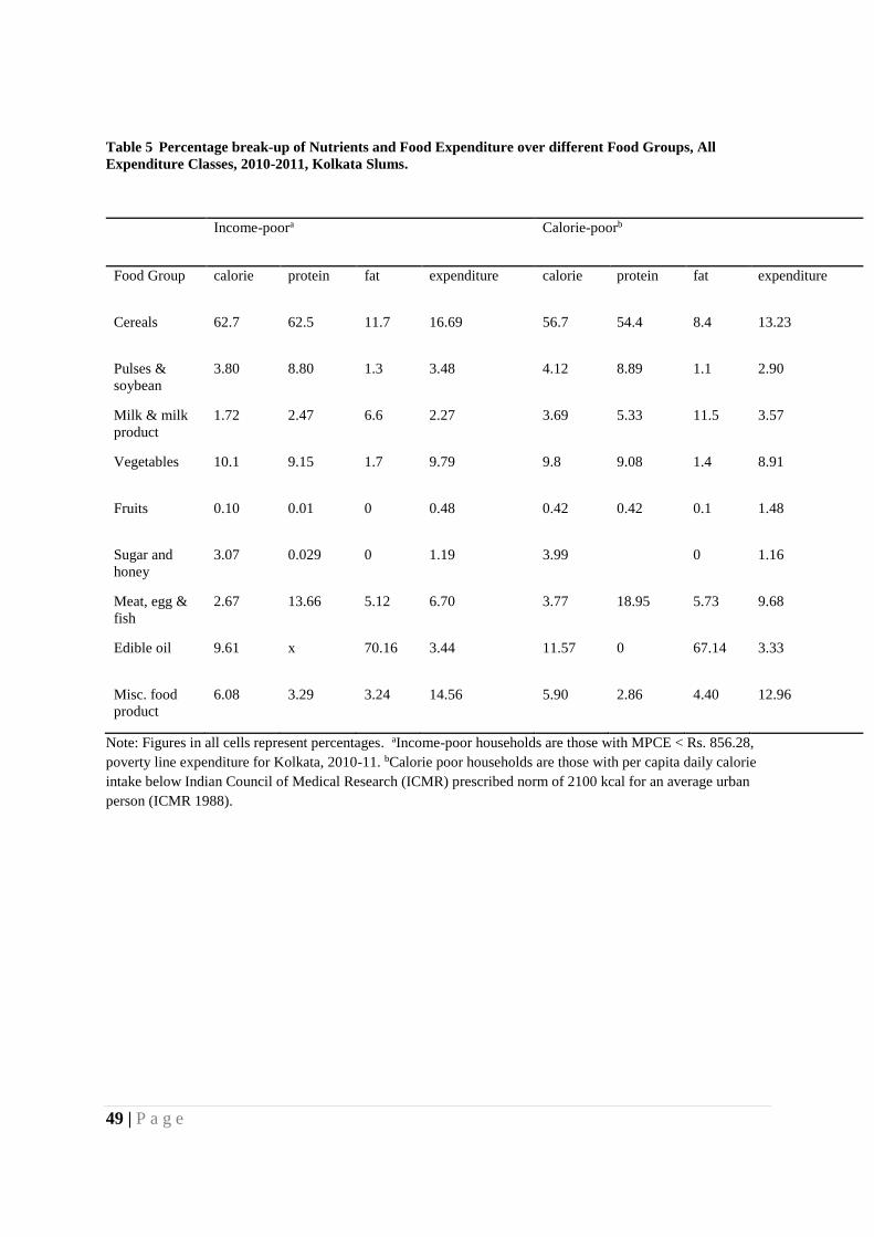
49 | P a g e
Table 5 Percentage break-up of Nutrients and Food Expenditure over different Food Groups, All
Expenditure Classes, 2010-2011, Kolkata Slums.
Income-poora
Calorie-poorb
Food Group calorie protein fat expenditure calorie protein fat expenditure
Cereals 62.7 62.5 11.7 16.69 56.7 54.4 8.4 13.23
Pulses &
soybean
3.80 8.80 1.3 3.48 4.12 8.89 1.1 2.90
Milk & milk
product
1.72 2.47 6.6 2.27 3.69 5.33 11.5 3.57
Vegetables 10.1 9.15 1.7 9.79 9.8 9.08 1.4 8.91
Fruits 0.10 0.01 0 0.48 0.42 0.42 0.1 1.48
Sugar and
honey
3.07 0.029 0 1.19 3.99 0 1.16
Meat, egg &
fish
2.67 13.66 5.12 6.70 3.77 18.95 5.73 9.68
Edible oil 9.61 x 70.16 3.44 11.57 0 67.14 3.33
Misc. food
product
6.08 3.29 3.24 14.56 5.90 2.86 4.40 12.96
Note: Figures in all cells represent percentages. aIncome-poor households are those with MPCE < Rs. 856.28,
poverty line expenditure for Kolkata, 2010-11. bCalorie poor households are those with per capita daily calorie
intake below Indian Council of Medical Research (ICMR) prescribed norm of 2100 kcal for an average urban
person (ICMR 1988).
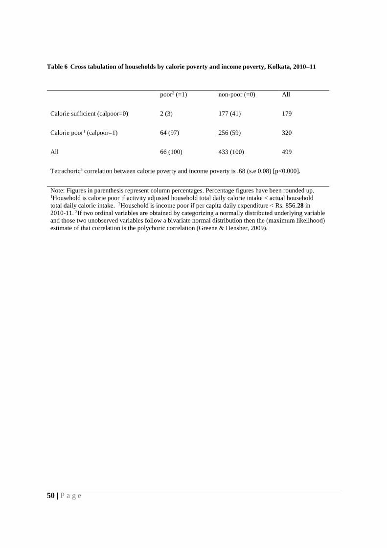
50 | P a g e
Table 6 Cross tabulation of households by calorie poverty and income poverty, Kolkata, 2010–11
poor2 (=1) non-poor (=0) All
Calorie sufficient (calpoor=0) 2 (3) 177 (41) 179
Calorie poor1 (calpoor=1) 64 (97) 256 (59) 320
All 66 (100) 433 (100) 499
Tetrachoric3 correlation between calorie poverty and income poverty is .68 (s.e 0.08) [p<0.000].
Note: Figures in parenthesis represent column percentages. Percentage figures have been rounded up. 1Household is calorie poor if activity adjusted household total daily calorie intake < actual household
total daily calorie intake. 2Household is income poor if per capita daily expenditure < Rs. 856.28 in
2010-11. 3If two ordinal variables are obtained by categorizing a normally distributed underlying variable
and those two unobserved variables follow a bivariate normal distribution then the (maximum likelihood)
estimate of that correlation is the polychoric correlation (Greene & Hensher, 2009).
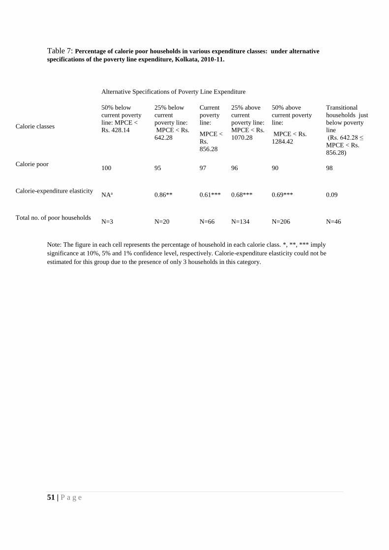
51 | P a g e
Table 7: Percentage of calorie poor households in various expenditure classes: under alternative
specifications of the poverty line expenditure, Kolkata, 2010-11.
Note: The figure in each cell represents the percentage of household in each calorie class. *, **, *** imply
significance at 10%, 5% and 1% confidence level, respectively. Calorie-expenditure elasticity could not be
estimated for this group due to the presence of only 3 households in this category.
Alternative Specifications of Poverty Line Expenditure
Calorie classes
50% below
current poverty
line: MPCE <
Rs. 428.14
25% below
current
poverty line:
MPCE < Rs.
642.28
Current
poverty
line:
MPCE <
Rs.
856.28
25% above
current
poverty line:
MPCE < Rs.
1070.28
50% above
current poverty
line:
MPCE < Rs.
1284.42
Transitional
households just
below poverty
line
(Rs. 642.28 ≤
MPCE < Rs.
856.28)
Calorie poor
100 95 97 96 90 98
Calorie-expenditure elasticity NAa 0.86** 0.61*** 0.68*** 0.69*** 0.09
Total no. of poor households N=3 N=20 N=66 N=134 N=206 N=46

52 | P a g e
Table 8: Percentage of calorie poor households in various expenditure classes: under alternative
specifications of the poverty line expenditure, Kolkata, 2010-11.
.
Note: The figure in each cell represents the percentage of household in each calorie class. *, **, *** imply
significance at 10%, 5% and 1% confidence level, respectively.
Alternative Specifications of Poverty Line Expenditure
Calorie classes
50% below
current
poverty line:
MPCE ≥ Rs.
428.14
25% below
current
poverty line:
MPCE ≥ Rs.
642.28
Current
poverty line:
MPCE ≥ Rs.
856.28
25% above
current poverty
line:
MPCE ≥ Rs.
1070.28
50%
above
current
poverty
line:
MPCE ≥
Rs.
1284.42
Transitional
households
just above
poverty line
(Rs. 856.28≤
MPCE <
Rs. 1070.28)
calorie poor
64 63 60 52 46 96
Calorie-expenditure
elasticity 0.46*** 0.42*** 0.37** 0.33** 0.28** 0.33
Total no. of non-poor
households
N=496 N=479 N=433 N=365 N=293 N=68

53 | P a g e
Table 9 Marginal Effect of Income Poverty on Calorie poverty in Recursive Bivariate Probit Model, Kolkata, 2010-11
Recursive
Bivariate
Probit 1
poverty line expenditure
= 642.28 (25% below
official poverty line)2
poor (official poverty
line= Rs.856.28) poverty line expenditure
= 1070.35 (25% above
official poverty line)
poverty line expenditure
= 1284.35 (50% above
official poverty line) 3
calpoor NA 0.59***(0.18) 0.33 (0.18) 0.22**(0.10)3
fincal NA 0.60** (0.24) 0.21 (0.21) 0.28***(0.10)4
*, **, *** imply significance at 10%, 5% and 1% confidence level, respectively. N=499. Robust standard errors
in parenthesis. 1Control variables are: household size, age, gender, religion, education and homeownership
status of households and household composition. Additionally, poverty equation includes household asset
ownership status, household employment status and logarithm of non-food expenditure as identifying variables. 2 Bivariate probit model could not be estimated due to small number of observations in poor. 3 Rho is significant
at 10% level of significance for this level of poverty line expenditure. Detailed result reported in Appendix.
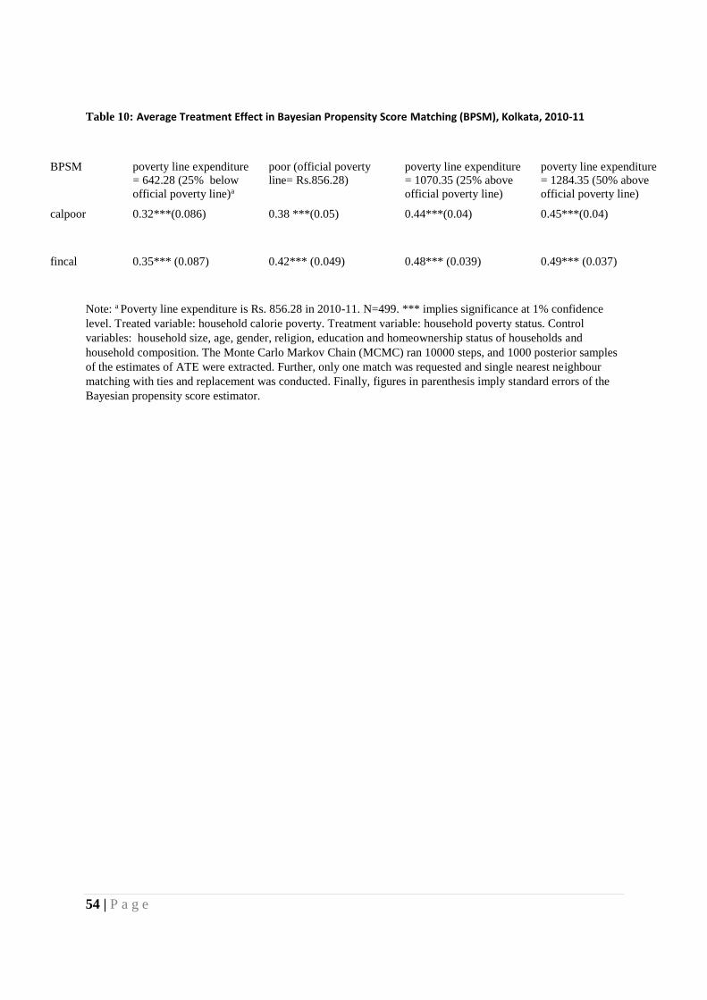
54 | P a g e
Table 10: Average Treatment Effect in Bayesian Propensity Score Matching (BPSM), Kolkata, 2010-11
BPSM poverty line expenditure
= 642.28 (25% below
official poverty line)a
poor (official poverty
line= Rs.856.28) poverty line expenditure
= 1070.35 (25% above
official poverty line)
poverty line expenditure
= 1284.35 (50% above
official poverty line)
calpoor 0.32***(0.086) 0.38 ***(0.05) 0.44***(0.04) 0.45***(0.04)
fincal 0.35*** (0.087) 0.42*** (0.049) 0.48*** (0.039) 0.49*** (0.037)
Note: a Poverty line expenditure is Rs. 856.28 in 2010-11. N=499. *** implies significance at 1% confidence
level. Treated variable: household calorie poverty. Treatment variable: household poverty status. Control
variables: household size, age, gender, religion, education and homeownership status of households and
household composition. The Monte Carlo Markov Chain (MCMC) ran 10000 steps, and 1000 posterior samples
of the estimates of ATE were extracted. Further, only one match was requested and single nearest neighbour
matching with ties and replacement was conducted. Finally, figures in parenthesis imply standard errors of the
Bayesian propensity score estimator.

55 | P a g e
Figure 1: Kernel Distribution of Average Daily Calorie Intake and MPCE, All Households (N=499), Kolkata,
2010-11.
0.5
11.5
De
nsity
5 6 7 8 9Logarithm of MPCE and Per Capita Daily Calorie Intake
Log MPCE
Log Per Capita Daily Calories
kernel = epanechnikov, bandwidth = 0.1255
Distribution of Average Daily Calorie Intake and MPCE: ALL Households
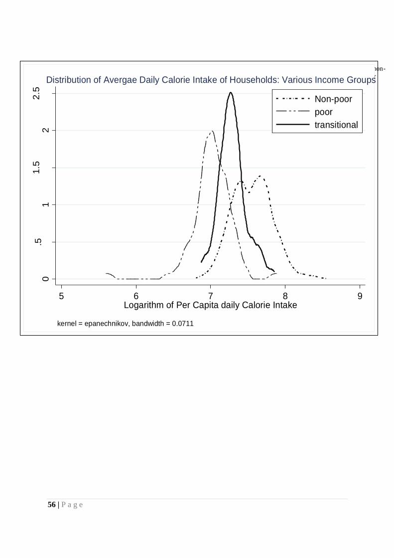
56 | P a g e
Figure 2: Distribution of Average Daily Calorie Intake of Households by Income Groups: poor with MPCE< Rs. 856.28 (N=66), non-
poor with MPCE> Rs. 856.28 and Transitional Households (Rs. 856.28<=MPCE< Rs. 1070) (N=68), Kolkata 2010-11. Note: Poor
households are those with MPCE<Rs.856.28.
0.5
11.5
22.5
De
nsity
5 6 7 8 9Logarithm of Per Capita daily Calorie Intake
Non-poor
poor
transitional
kernel = epanechnikov, bandwidth = 0.0711
Distribution of Avergae Daily Calorie Intake of Households: Various Income Groups

57 | P a g e
A. Lowess Plot of Calorie-Expenditure, All Households (N=499), Kolkata 2010-11.
B. Lowess Plot of Calorie-Expenditure for the
poor households MPCE<Rs.856.28 (N=66).
C. Lowess Plot of Calorie-Expenditure for the
Transitional households above poverty line (856.28≤
MPCE≤1070.35) (N=68).
5.5
66.5
77.5
8
Lo
ga
rith
m o
f P
er
Cap
ita
Daily C
alo
rie
Inta
ke
5.5 6 6.5 7Logarithm of MPCE
bandwidth = .8
Calorie-Expenditure Plot: Poor Households
6.8
77.2
7.4
7.6
7.8
Lo
ga
rith
m o
f P
er
Cap
ita
Daily
Ca
lorie
Inta
ke
6.8 7 7.2 7.4Logarithm of MPCE
bandwidth = .7
Calorie-Expenditure Plot: Transitional Households
56
78
9
Loga
rithm
of P
er C
apita
Dai
ly C
alor
ie In
take
5 6 7 8 9Logarithm of MPCE
bandwidth = .8
Calorie-Expenditure Plot: All Households
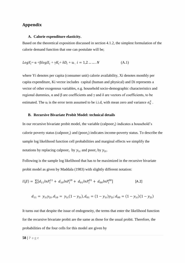
58 | P a g e
Appendix
A. Calorie expenditure elasticity.
Based on the theoretical exposition discussed in section 4.1.2, the simplest formulation of the
calorie demand function that one can postulate will be;
𝐿𝑜𝑔𝑌𝑖= α +β𝑙𝑜𝑔𝑋𝑖 + γ𝐾𝑖+ δ𝐷𝑖 + ui , 𝑖 = 1,2 … … . 𝑁 (A.1)
where Yi denotes per capita (consumer unit) calorie availability, Xi denotes monthly per
capita expenditure, Ki vector includes capital (human and physical) and Di represents a
vector of other exogenous variables, e.g. household socio-demographic characteristics and
regional dummies, α and β are coefficients and γ and δ are vectors of coefficients, to be
estimated. The ui is the error term assumed to be i.i.d, with mean zero and variance 𝜎𝑢2 .
B. Recursive Bivariate Probit Model: technical details
In our recursive bivariate probit model, the variable (calpoori) indicates a household’s
calorie poverty status (calpoori) and (poori) indicates income-poverty status. To describe the
sample log likelihood function cell probabilities and marginal effects we simplify the
notations by replacing calpoori by 𝑦1𝑖 and poori by 𝑦2𝑖.
Following is the sample log likelihood that has to be maximized in the recursive bivariate
probit model as given by Maddala (1983) with slightly different notation:
𝑙(𝛽) = ∑[𝑑11𝑙𝑛𝑃𝑖11 + 𝑑10𝑙𝑛𝑃𝑖
10 + 𝑑01𝑙𝑛𝑃𝑖01 + 𝑑00𝑙𝑛𝑃𝑖
00] [A.2]
𝑑11 = 𝑦1𝑖𝑦2𝑖, 𝑑10 = 𝑦1𝑖(1 − 𝑦2𝑖), 𝑑01 = (1 − 𝑦1𝑖)𝑦2𝑖; 𝑑00 = (1 − 𝑦1𝑖)(1 − 𝑦2𝑖)
It turns out that despite the issue of endogeneity, the terms that enter the likelihood function
for the recursive bivariate probit are the same as those for the usual probit. Therefore, the
probabilities of the four cells for this model are given by
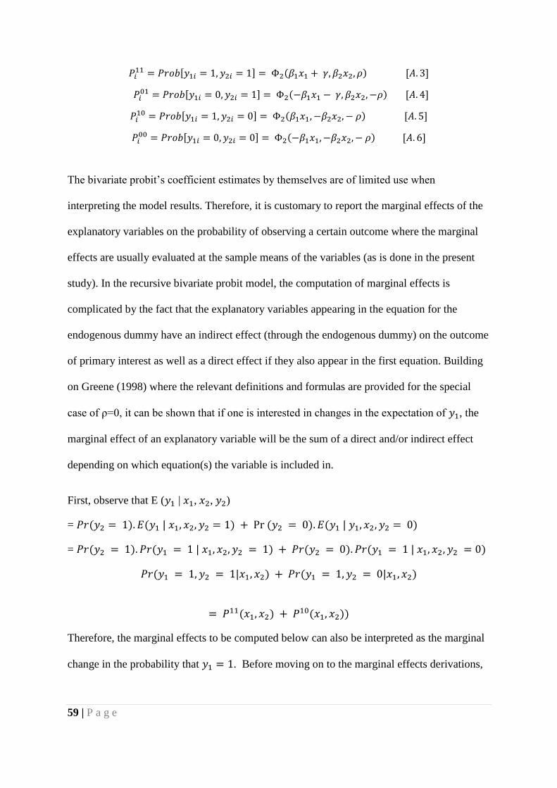
59 | P a g e
𝑃𝑖11 = 𝑃𝑟𝑜𝑏[𝑦1𝑖 = 1, 𝑦2𝑖 = 1] = Φ2(𝛽1𝑥1 + 𝛾, 𝛽2𝑥2, 𝜌) [𝐴. 3]
𝑃𝑖01 = 𝑃𝑟𝑜𝑏[𝑦1𝑖 = 0, 𝑦2𝑖 = 1] = Φ2(−𝛽1𝑥1 − 𝛾, 𝛽2𝑥2, −𝜌) [𝐴. 4]
𝑃𝑖10 = 𝑃𝑟𝑜𝑏[𝑦1𝑖 = 1, 𝑦2𝑖 = 0] = Φ2(𝛽1𝑥1, −𝛽2𝑥2, − 𝜌) [𝐴. 5]
𝑃𝑖00 = 𝑃𝑟𝑜𝑏[𝑦1𝑖 = 0, 𝑦2𝑖 = 0] = Φ2(−𝛽1𝑥1, −𝛽2𝑥2, − 𝜌) [𝐴. 6]
The bivariate probit’s coefficient estimates by themselves are of limited use when
interpreting the model results. Therefore, it is customary to report the marginal effects of the
explanatory variables on the probability of observing a certain outcome where the marginal
effects are usually evaluated at the sample means of the variables (as is done in the present
study). In the recursive bivariate probit model, the computation of marginal effects is
complicated by the fact that the explanatory variables appearing in the equation for the
endogenous dummy have an indirect effect (through the endogenous dummy) on the outcome
of primary interest as well as a direct effect if they also appear in the first equation. Building
on Greene (1998) where the relevant definitions and formulas are provided for the special
case of ρ=0, it can be shown that if one is interested in changes in the expectation of 𝑦1, the
marginal effect of an explanatory variable will be the sum of a direct and/or indirect effect
depending on which equation(s) the variable is included in.
First, observe that E (𝑦1 | 𝑥1, 𝑥2, 𝑦2)
= 𝑃𝑟(𝑦2 = 1). 𝐸(𝑦1 | 𝑥1, 𝑥2, 𝑦2 = 1) + Pr (𝑦2 = 0). 𝐸(𝑦1 | 𝑦1, 𝑥2, 𝑦2 = 0)
= 𝑃𝑟(𝑦2 = 1). 𝑃𝑟(𝑦1 = 1 | 𝑥1, 𝑥2, 𝑦2 = 1) + 𝑃𝑟(𝑦2 = 0). 𝑃𝑟(𝑦1 = 1 | 𝑥1, 𝑥2, 𝑦2 = 0)
𝑃𝑟(𝑦1 = 1, 𝑦2 = 1|𝑥1, 𝑥2) + 𝑃𝑟(𝑦1 = 1, 𝑦2 = 0|𝑥1, 𝑥2)
= 𝑃11(𝑥1, 𝑥2) + 𝑃10(𝑥1, 𝑥2))
Therefore, the marginal effects to be computed below can also be interpreted as the marginal
change in the probability that 𝑦1 = 1. Before moving on to the marginal effects derivations,
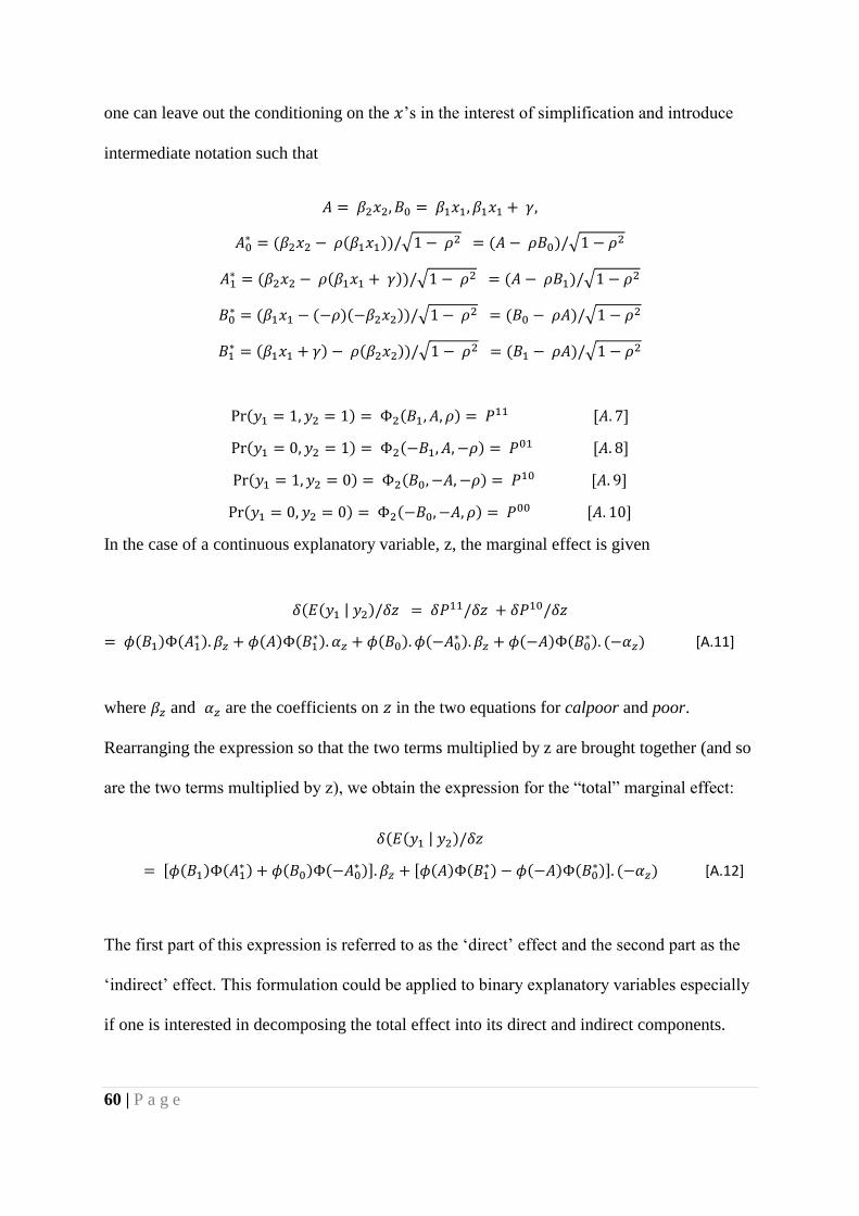
60 | P a g e
one can leave out the conditioning on the 𝑥’s in the interest of simplification and introduce
intermediate notation such that
𝐴 = 𝛽2𝑥2, 𝐵0 = 𝛽1𝑥1, 𝛽1𝑥1 + 𝛾,
𝐴0∗ = (𝛽2𝑥2 − 𝜌(𝛽1𝑥1))/√1 − 𝜌2 = (𝐴 − 𝜌𝐵0)/√1 − 𝜌2
𝐴1∗ = (𝛽2𝑥2 − 𝜌(𝛽1𝑥1 + 𝛾))/√1 − 𝜌2 = (𝐴 − 𝜌𝐵1)/√1 − 𝜌2
𝐵0∗ = (𝛽1𝑥1 − (−𝜌)(−𝛽2𝑥2))/√1 − 𝜌2 = (𝐵0 − 𝜌𝐴)/√1 − 𝜌2
𝐵1∗ = (𝛽1𝑥1 + 𝛾) − 𝜌(𝛽2𝑥2))/√1 − 𝜌2 = (𝐵1 − 𝜌𝐴)/√1 − 𝜌2
Pr(𝑦1 = 1, 𝑦2 = 1) = Φ2(𝐵1, 𝐴, 𝜌) = 𝑃11 [𝐴. 7]
Pr(𝑦1 = 0, 𝑦2 = 1) = Φ2(−𝐵1, 𝐴, −𝜌) = 𝑃01 [𝐴. 8]
Pr(𝑦1 = 1, 𝑦2 = 0) = Φ2(𝐵0, −𝐴, −𝜌) = 𝑃10 [𝐴. 9]
Pr(𝑦1 = 0, 𝑦2 = 0) = Φ2(−𝐵0, −𝐴, 𝜌) = 𝑃00 [𝐴. 10]
In the case of a continuous explanatory variable, z, the marginal effect is given
𝛿(𝐸(𝑦1 | 𝑦2)/𝛿𝑧 = 𝛿𝑃11/𝛿𝑧 + 𝛿𝑃10/𝛿𝑧
= 𝜙(𝐵1)Φ(𝐴1∗ ). 𝛽𝑧 + 𝜙(𝐴)Φ(𝐵1
∗). 𝛼𝑧 + 𝜙(𝐵0). 𝜙(−𝐴0∗ ). 𝛽𝑧 + 𝜙(−𝐴)Φ(𝐵0
∗). (−𝛼𝑧) [A.11]
where 𝛽𝑧 and 𝛼𝑧 are the coefficients on 𝑧 in the two equations for calpoor and poor.
Rearranging the expression so that the two terms multiplied by z are brought together (and so
are the two terms multiplied by z), we obtain the expression for the “total” marginal effect:
𝛿(𝐸(𝑦1 | 𝑦2)/𝛿𝑧
= [𝜙(𝐵1)Φ(𝐴1∗ ) + 𝜙(𝐵0)Φ(−𝐴0
∗ )]. 𝛽𝑧 + [𝜙(𝐴)Φ(𝐵1∗) − 𝜙(−𝐴)Φ(𝐵0
∗)]. (−𝛼𝑧) [A.12]
The first part of this expression is referred to as the ‘direct’ effect and the second part as the
‘indirect’ effect. This formulation could be applied to binary explanatory variables especially
if one is interested in decomposing the total effect into its direct and indirect components.

61 | P a g e
However, a more accurate definition for the total marginal effect of a binary variable q,
which belongs in in 𝑥1 and/or 𝑥2, is
𝐸(𝑦1|𝑦2, 𝑞 = 1) − 𝐸(𝑦1|𝑦2, 𝑞 = 0) = [𝑃11(𝑞 = 1) + 𝑃10(𝑞 = 1)] − [𝑃11(𝑞 = 0) + 𝑃10(𝑞 = 0)]
[A.13]
where 𝑃𝑖𝑗 (𝑞 = 𝑘) denotes 𝑃𝑖𝑗 calculated at 𝑞 = 𝑘.
Finally, the marginal effect of the endogenous binary variable 𝑦2, is defined in terms of
univariate normal probabilities since,
𝐸(𝑦1|𝑦2 = 1) − 𝐸(𝑦1|𝑦2 = 0) = Φ(𝐵1) − Φ(𝐵0) [𝐴. 14]
Since the expectation of 𝑦2 is conditioned only on 𝑥2, i.e. 𝐸[𝑦2|𝑥2] = 𝑃𝑟 [𝑦2 = Φ(𝐴)],
marginal effects for this equation are also defined in terms of univariate normal probabilities
as in the univariate probit model. Calculation of the marginal effects is useful since it may
turn out that, in all instances, the coefficients on the same variable have the opposite signs in
the two equations, meaning that the total (or net) effect of the variable needs to be computed
to determine the sign as well as the size of the impact of an explanatory variable.
C. Further on Bayesian Propensity Score Matching
The posterior joint distribution of the ATE ( ) and the parameters , of the BPSM16 can
be written as
2 2, , , , (1) , (0) , , , ,i i i if X D Calpoor f Calpoor f Calpoor f D X
(C)
where
16 The main difference between BPSM and PSM is that the former performs stochastic matching while in the
latter the matching is done in a deterministic manner.

62 | P a g e
2(1) , 0 ,i i i i
i T
f Calpoor N Calpoor Calpoor
[A.15]
2(0) , 1 ,i i i i
i C
f Calpoor N Calpoor Calpoor
[A.16]
1
1
, 1ii
NDD
i i
i
f D X G X G X
[A.17]
where 2, ,i i is the prior and i iG X p is the predicted propensity score based on
logit function. It is important to note equation (A.15) implies that the observed outcome for
the treated unit follows a normal distribution with mean 0i iCalpoor and variance 2
i and
equation (A.16) implies that the observed outcome for the control unit follows a normal
distribution with mean 1i iCalpoor and variance 2
i . In (A.15) and (A.16) 0iCalpoor
and 1iCalpoor respectively are the imputed outcomes defined in Eq.12 and Eq. 13. In order
to obtain the estimate of ATE its marginal posterior distribution can be approximated by
employing the posterior samples generated by the Markov chain Monte Carlo (MCMC)
method.