income inequality in italy: facts and measurementold.sis-statistica.org/files/pdf/atti/atti...
TRANSCRIPT

Income Inequality in Italy: Facts and Measurement(*) La disuguaglianza dei redditi in Italia: fatti e misure
Andrea Brandolini
Bank of Italy, Department for Structural Economic Analysis e-mail: [email protected]
Riassunto: Il lavoro esamina la distribuzione del reddito in Italia, la sua evoluzione nel tempo e la sua struttura nel confronto internazionale. Passate brevemente in rassegna le fonti principali, sono discussi alcuni problemi statistici che emergono dal loro raffronto. Si mostra che nei primi anni ottanta è terminata una fase di significativa compressione della distribuzione. Nei due decenni seguenti la disuguaglianza è aumentata, sebbene in misura minore di quanto avvenuto in altre economie avanzate. Il confronto internazionale evidenzia che l’Italia rimane tuttavia uno dei paesi ricchi con la distribuzione più sperequata. Tre fattori sembrano incidere più di altri su questo risultato: la bassa partecipazione al mercato del lavoro, una politica redistributiva pubblica poco efficace nel ridurre le disuguaglianze originarie, gli amplissimi squilibri territoriali.
Keywords: income distribution, inequality, poverty, Italy, North-South divide
1. Introduction
The study of the personal distribution of income has a long, yet erratic, tradition in Italian economics and statistics. The intense international debate ignited at the end of the 19th century by Pareto’s analysis of the revenue curve saw the participation of many Italian scholars: Amoroso, Benini, Bresciani-Turroni, D’Addario, Gini, Mortara, Pietra, Ricci, Savorgnan, Vinci, to name just a few. Significantly, it was to a leading Italian economist like Bresciani-Turroni that the editors of Econometrica turned to write the survey that put a virtual end to the debate (1939). It was in the course of that debate that Gini (1912) came to elaborate the index named after him that was to become the most popular statistics world-wide to measure inequality.
There was some interest for the subject in the late 1940s, when Luzzato Fegiz (1950) carried out the Doxa survey under the impulse of Einaudi and Del Vecchio, but it then followed a long period of oblivion. The last two decades have gradually seen a renewed attention for the way incomes are distributed among Italians, in part for the possibility to access household-level data in various sources, in part for the growing concern that inequalities are on the rise. Household impoverishment and disappearing middle class are nowadays at the centre of the Italian public debate.
In this paper, I investigate the personal distribution of income in Italy. After a brief description of available sources in Section 2, I document the temporal evolution of income inequality during the last thirty years in Section 3 and discuss some statistical problems in Section 4. I sketch an international comparison showing the position of Italy among advanced countries in Section 5, and I then move to a detailed comparison (*) The views expressed herein are mine and do not necessarily reflect those of the Bank of Italy.
– 55 –

of the distributions of income in Italy, Germany, and the United States in Section 6, in order to identify the factors that could account for the high level of inequality in Italy. I draw some conclusions in the last Section.
2. Sources on the distribution of household incomes
The Bank of Italy’s Survey of Household Income and Wealth (SHIW) has been the main source on the distribution of personal incomes in Italy since the late 1960s (Brandolini, 1999; Banca d’Italia, 2008). The SHIW has been widely used to study the economic behavior of Italian households, but it must be borne in mind that temporal comparisons are hampered by modifications in the design and the definition of income; in part, these discontinuities can be kept under control by using the individual data stored in the survey Historical Archive (SHIW-HA), which covers the waves from 1977 onwards (microdata of previous waves are no longer available). The SHIW data are included in the Luxembourg Income Study (LIS), an international database containing harmonized social and economic data from household surveys collected in thirty countries (http://www.lisproject.org; Smeeding, 2004).
Only recently Istat has started to collect detailed income information at the household level. From 1994 to 2001, Istat carried out the European Community Household Panel (ECHP), the Italian section of a longitudinal household survey coordinated by Eurostat to gather information on personal income and living standards in the European Union. The eight waves of the ECHP contain household incomes in the period 1993-2000. Since 2004, Istat conducts a yearly household survey which provides the data for the European Statistics on Income and Living Conditions (EU-SILC) project. The aim of this project is to become the EU reference source for comparative statistics on income distribution and social exclusion at the European level, particularly in the context of the EU social inclusion process and monitoring of the progress towards greater social cohesion (Clemenceau and Museux, 2007). The EU-SILC sample size is about three times that of the other two surveys, around 24,000 households against 8,000 and 7,000 households for the SHIW and the ECHP, respectively. In order to improve the quality of the results, Istat has implemented a new procedure based on the linkage of survey data to administrative records (Di Marco, 2007).
3. The time pattern of income inequality in the last thirty years
Estimates of the Gini index for disposable income are collected in Table 1. The first four columns contain the statistics from the SHIW, computed on grouped data before 1977 and on microdata from the SHIW-HA thereafter. The three reported definitions of income include all revenues from employment, self-employment, pension and social assistance, net of taxes and social security contributions, but differ for the coverage of imputed rents for owner-occupied dwellings, and interest and dividends. To account for the economies of scale from cohabitation, incomes are equivalized by means of the “square root” equivalence scale, which takes the number of equivalent adults to be equal to the square root of the household size (Atkinson, Rainwater and Smeeding,
– 56 –
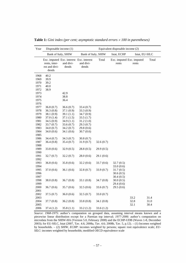
Table 1: Gini index (per cent; asymptotic standard errors × 100 in parentheses)
Year Disposable income (1) Equivalent disposable income (2)
Bank of Italy, SHIW Bank of Italy, SHIW Istat, ECHP Istat, EU-SILC
Exc. imputed rents, inter-est and divi-
dends
Exc. interest and divi-
dends
Exc. interest and divi-
dends
Total Exc. imputed rents
Exc. imputed rents
Total
1968 40.2 1969 39.9 1970 39.2 1971 40.0 1972 38.9 1973 42.9 1974 38.8 1975 36.4 1976 1977 36.8 (0.7) 36.6 (0.7) 33.4 (0.7) 1978 36.3 (0.8) 37.1 (0.9) 33.3 (0.9) 1979 38.1 (0.9) 39.1 (1.1) 34.7 (0.9) 1980 37.0 (1.4) 37.1 (1.5) 33.5 (1.7) 1981 34.5 (0.9) 34.9 (1.1) 31.2 (1.0) 1982 33.7 (0.7) 33.6 (0.7) 29.3 (0.7) 1983 34.0 (0.7) 34.2 (0.7) 29.8 (0.6) 1984 34.0 (0.6) 34.1 (0.6) 30.7 (0.6) 1985 1986 34.4 (0.7) 34.3 (0.7) 30.8 (0.7) 1987 36.4 (0.8) 35.4 (0.7) 31.9 (0.7) 32.6 (0.7) 1988 1989 33.8 (0.6) 32.9 (0.5) 28.8 (0.5) 29.9 (0.5) 1990 1991 32.7 (0.7) 32.2 (0.7) 28.0 (0.6) 29.1 (0.6) 1992 1993 36.8 (0.6) 35.8 (0.6) 32.2 (0.6) 33.7 (0.6) 32.7 (0.5) 1994 33.0 (0.6) 1995 37.0 (0.6) 36.1 (0.6) 32.8 (0.7) 33.9 (0.7) 31.7 (0.5) 1996 30.6 (0.5) 1997 30.4 (0.5) 1998 38.0 (0.8) 36.7 (0.8) 33.1 (0.8) 34.7 (0.8) 30.0 (0.5) 1999 29.4 (0.6) 2000 36.7 (0.6) 35.7 (0.6) 32.5 (0.6) 33.6 (0.7) 29.5 (0.6) 2001 2002 37.5 (0.7) 36.0 (0.6) 32.5 (0.7) 33.0 (0.7) 2003 33.2 31.4 2004 37.7 (0.8) 36.2 (0.8) 33.8 (0.8) 34.1 (0.8) 32.8 31.0 2005 32.1 30.4 2006 37.4 (1.2) 35.8 (1.1) 33.2 (1.2) 33.6 (1.2)
Source: 1968-1975: author’s computation on grouped data, assuming interval means known and a piecewise linear distribution except for a Paretian top interval; 1977-2006: author’s computation on microdata from the SHIW-HA (Version 5.0, February 2008) and the ECHP-UDB (Waves 1-8, December 2003); for EU-SILC, Istat (2007, Tav. 4.6; 2008a, Tav. 4.6; 2008b, Tav. 5, p.12). – (1) Incomes weighted by households. – (2) SHIW, ECHP: incomes weighted by persons; square root equivalence scale; EU-SILC: incomes weighted by households; modified OECD equivalence scale
– 57 –

1995). Each household’s income is counted once to derive unequivalized figures (household weights) and as many times as the number of household’s members to obtain equivalized figures (person weights). The latter distribution is currently the one most common in national and international statistics: it amounts to take the individual as the reference welfare unit, under the assumption that resources are shared and equally divided within the household; the equivalent income can be seen as the per capita income augmented to embody the gains from the economies of scale. The fifth column of the Table contains statistics for all eight waves of the ECHP computed from the User Data Base (UDB). All estimates refer to the distribution of equivalent disposable incomes among persons, where total household income is the sum of the monetary incomes of all adult members net of income taxes and social security contributions, excluding imputed rents for owner-occupied dwellings, and fringe benefits and other non-cash compensation.To facilitate comparison with the SHIW statistics, the ECHP estimates are calculated using the square root equivalence scale instead of the modified OECD scale recommended by Eurostat. In all cases, standard errors are calculated under the simplifying assumption of simple random sampling. The last two columns of Table 1 report published figures from the EU-SILC. The EU-SILC definition coincides with that of the ECHP, except for the inclusion of the imputed value for company cars; the two reported series differ for the coverage of the imputed rent for owner-occupied dwellings (net of ordinary maintenance expenses and interest payments on the mortgage where they exist). The EU-SILC statistics are based on the modified OECD equivalence scale and are weighted by households.
According to the SHIW evidence, from the early 1970s to 1982, with the exception of 1978-1979, the inequality of household disposable incomes fell considerably (Figure 1). It remained rather stable in the mid-1980s, it grew in 1987, and it declined further in 1989-1991. A sharp increase between 1991 and 1993 brought the Gini index back to the value of 1980. Since then, the Gini index has exhibited some fluctuations, but no steady tendency to increase or decrease: for instance, the rise in 1998 was reversed within the next two years. These phases correspond to statistically significant changes: considering the figures reported in the first four columns of Table 1, 13 out of the 14 pair comparisons 1977-1982, 1982-1987, 1987-1991 and 1991-1993 are significant at the 1 percent level. Between 1993 and 2006, on the other hand, none of the pairwise comparisons is statistically significant.
Like all summary measures of inequality, the Gini index may conceal divergent movements at different points of the distribution. Hence, Figure 2 plots the income shares of each fifth of the population ranked by increasing income, calculated for the same concepts of income used in Table 1. The dynamics of the income shares of the top population fifth were very close to those of the Gini index. Focusing on disposable incomes excluding interest and dividends, between 1973 and 2006 the share of the top fifth fell by almost 6 percentage points to the benefit of all other fifths. During the 1970s, the largest gains accrued to the bottom and, to a lesser extent, second fifths; except for a drop in 1987, from 1980 to 1991 these shares remained fairly stable at around 7 and 12 per cent, respectively; in 1993 they fell to the values of 1980. The income share of the bottom fifth partly recovered from 1998 to 2006, while that of the second fifth remained fairly stable throughout the period. The shares of the third and fourth fifths exhibited somewhat smaller changes, and tended to increase up to the early 1990s and to decrease afterwards. Similar patterns characterize the other income concepts.
– 58 –

The story told by the ECHP data for the 1990s is different. The Gini index fell steadily, from around 33 percent in 1993 and 1994 to about 29.5 in 1999 and 2000 (Figure 1). The drop is statistically significant, and would not change by using instead the modified OECD equivalence scale. The leveling of the distribution was caused by the growth in the income shares of the bottom 60 percent of the population at the expense of the remaining 40 percent (Figure 2). The poorest fifth gained 1.0 percentage points, whereas the richest fifth lost over 2.2 percentage points.
Figure 1: Gini index (per cent)
28
30
32
34
36
38
40
42
44
1965 1970 1975 1980 1985 1990 1995 2000 2005 2010
SHIW, disposable income, exc. imputed rents, interest and dividends, householdsSHIW, disposable income, exc. interest and dividends, householdsSHIW, equivalent disposable income (square root scale), personsECHP, equivalent disposable income (square root scale), personsEU-SILC, equivalent disposable income (modified OECD scale), households
Source: see Table 1
Lastly, Figure 3 plots the proportion of low-income persons, defined as those people with equivalent income below some predetermined fraction of the median equivalent income. Three different cut-offs are indicated in the Figure: 50, 60 and 70 percent of the median. The movements of the share of low-income persons basically mimic those of the Gini index. According to the SHIW data, with a threshold at 50 or 60 percent of median income, the smallest proportion of low-income persons since 1977 is found in 1981; it follows an upward trend until 1987, a new low in 1989, and an abrupt rise from 1991 to 1993; the share of persons with low income has remained virtually unchanged afterwards. Raising the cut-off at 70 percent of the median yields a somewhat different pattern over time. There is not much change from 1977 to 1991, save for the large drop between 1980 and 1981 and its quick reversal by 1984. The upsurge in 1993 brings the proportion of low-income persons at a much higher level than in previous years, but it is succeeded by a falling, rather than stationary, tendency in the next period. As for the
– 59 –
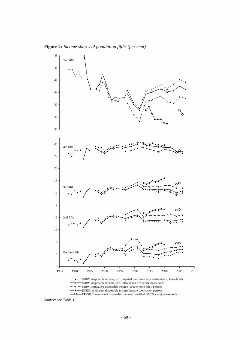
Figure 2: Income shares of population fifths (per cent)
36
38
40
42
44
46
48Top fifth
4
6
8
10
12
14
16
18
20
22
24
1965 1970 1975 1980 1985 1990 1995 2000 2005 2010
Bottom fifth
2nd fifth
4th fifth
3rd fifth
SHIW, disposable income, exc. imputed rents, interest and dividends, householdsSHIW, disposable income, exc. interest and dividends, householdsSHIW, equivalent disposable income (square root scale), personsECHP, equivalent disposable income (square root scale), personsEU-SILC, equivalent disposable income (modified OECD scale), households
Source: see Table 1.
– 60 –

Gini index, the ECHP portrays a somewhat different picture from the SHIW. Whereas the SHIW suggests stability, the ECHP indicates a decline by about two percentage points from 1993 to 1998 which is almost entirely reversed in 1999 and 2000. The overall change is, however, similar in the two sources, as the estimated shares of low-income persons are fairly close at the beginning and the end of the period.
Figure 3: Share of low-income persons (per cent)
8
10
12
14
16
18
20
22
24
26
28
30
1975 1980 1985 1990 1995 2000 2005 2010
Below 70% of median
Below 50% of median
Below 60% of median
SHIW, equivalent disposable income, exc. interest and dividends (square root scale), personsSHIW, equivalent disposable income (square root scale), personsECHP, equivalent disposable income (square root scale), persons
Source: see Table 1 All in all, this evidence highlights various episodes in the evolution of income distribution. The “egalitarian” phase which had began in 1969 with the Autunno caldo (“Hot Autumn”) came to a halt in the early 1980s. This phase coincides with the post-war period in which industrial conflict was at its highest. Bargaining power shifted sharply in favor of workers and their strongly egalitarian demands, such as equal (lump-sum) pay raises for all employees regardless of grade. These demands translated into the 1975 reform of the wage indexation mechanism, which granted a flat-sum wage increase for each percentage point rise in the cost-of-living index. In the presence of double-digit inflation rates, the operation of this mechanism led to a strong narrowing of
– 61 –

the earnings structure throughout the early 1980s (Erickson and Ichino, 1995; Brandolini et al., 2002; Manacorda, 2004). This tendency propagated to the distribution of household incomes – at least in the data at our disposal which do not include interest and dividends. The following years saw some widening of the income distribution, but it was only at the time of the worst economic crisis of the post-war periods, between 1991 and 1993, that inequality and poverty rose sharply. No clear trends can be detected thereafter, in spite of considerable changes in the labor market, the system of social protection, and more generally the Italian society.
These observations suggest two considerations. First, there is no evidence yet of the rise in inequality, the household impoverishment, or the disappearance of the middle class which is often denounced in the public debate. This issue is analyzed in greater detail by Boeri and Brandolini (2004) and Brandolini (2005), but it is worth recollecting here that the apparent stability of the overall distribution documented above is the net result of divergent dynamics across social groups defined on the basis of the labor market status of the household head, with incomes growing more rapidly for self-employed and managers than for white- and blue-collars. Massari et al. (2008) provide further evidence of distributive changes within groups between 2000 and 2004 by using non parametric techniques. Second, the absence of a prolonged episode of rising income inequality is in contrast to the experience of many developed countries, such as the United States and the United Kingdom in the 1980s and Sweden and Finland in the 1990s (Brandolini and Smeeding, 2008a). It must be borne in mind, however, that the levels of inequality and poverty are among the highest measured in rich countries. Before turning to international comparisons, it is useful to outline some statistical problems and provide a tentative reconciliation of the conflicting evidence between the SHIW and the ECHP.
4. Explaining the conflicting evidence of the SHIW and the ECHP
The evolution of income distribution in the 1990s looks different depending on which source we utilize. Can this conflicting evidence be explained? The SHIW and the ECHP share some features, like size and stratification of the sample, but differ in two important respects: the formulation of the income questions, and the cross-sectional vs. longitudinal design.
A detailed comparison of the specification and phrasing of income questions in the two surveys is beyond the scope of this paper. Suffice it to say that the ECHP is more thorough than the SHIW in registering cash transfers received by the household, but it is much less detailed in recording earnings from self-employment, property income and capital income1. This diversity in the questionnaire leads to a rather different structure of average income, even after considering only items recorded in both surveys (Table 2). The ECHP mean falls short of the SHIW mean by over a fifth in all four years for
1 These incomes are recorded through single questions (at the household or individual level) in the ECHP and by means of several separate questions in the SHIW. For instance, in the last wave of the SHIW yields on financial wealth are derived by applying the average market return to the holdings of as many as 25 different categories of assets, while separate modules of the questionnaire, each containing about a dozen questions, are devoted to three categories of self-employed (members of arts or professions and persons working on own account; family businesses; active shareholders or partners).
– 62 –

Tab
le 2
: Com
pari
son
betw
een
the
ECH
P an
d th
e SH
IW in
com
e (th
ousa
nds o
f lir
e an
d pe
r cen
t)
Inco
me
com
pone
nt (a
)
1993
19
95
1998
20
00
EC
HP
SHIW
EC
HP
SHIW
EC
HP
SHIW
EC
HP
SHIW
EC
HP
SHIW
EC
HP
SHIW
EC
HP
SHIW
EC
HP
SHIW
Wag
es a
nd sa
larie
s 16
,305
16
,140
10
1 16
,555
16
,472
10
1 19
,114
17
,171
11
1 20
,724
18
,558
11
2 In
com
e fr
om se
lf-em
ploy
men
t 4,
462
7,04
4 63
5,
057
7,13
7 71
5,
787
9,10
1 64
6,
645
9,75
8 68
Pe
nsio
ns
7,33
3 8,
492
86
8,67
9 9,
996
87
10,6
24
11,2
14
95
11,3
75
11,8
36
96
O
ld-a
ge, s
urvi
vors
’ ben
efits
6,
640
8,05
6
9,
913
10,6
31
Si
ckne
ss, i
nval
idity
ben
efits
69
3
62
3
71
1
74
4
O
ther
tran
sfer
s 58
2 25
2 23
1 36
6 43
1 85
54
5 35
5 15
4 65
6 36
0 18
2
Une
mpl
oym
ent b
enef
its
275
191
310
388
Fa
mily
-rel
ated
allo
wan
ces
141
80
166
172
Ed
ucat
ion-
rela
ted
allo
wan
ces
55
36
22
44
A
ny o
ther
(per
sona
l) be
nefit
s 49
24
5
14
So
cial
ass
ista
nce
52
24
31
23
H
ousi
ng a
llow
ance
10
12
10
14
C
apita
l inc
ome
774
2,22
6 35
1,
296
2,05
7 63
77
8 2,
996
26
699
2,12
6 33
R
enta
l inc
ome
259
468
55
421
551
76
474
534
89
442
768
58
Tota
l dis
posa
ble
inco
me
(com
para
ble
defin
ition
) 29
,716
34
,622
86
32
,375
36
,644
88
37
,322
41
,371
90
40
,541
43
,407
93
Pr
ivat
e tra
nsfe
rs re
ceiv
ed
396
263
616
300
Adj
ustm
ent f
or n
on-r
espo
nse
(b)
96
105
179
228
Frin
ge b
enef
its o
f em
ploy
ees
10
0
15
7
15
2
18
5
Dep
reci
atio
n of
cap
ital g
oods
of t
he se
lf-em
ploy
ed (-
)
697
958
956
902
Pe
nsio
n ar
rear
s
126
67
156
84
In
tere
st p
ayab
le (-
)
539
630
318
350
Im
pute
d re
nts o
n ow
ner-
occu
pied
dw
ellin
gs
6,
275
7,75
8
8,
279
9,08
9
Tota
l dis
posa
ble
inco
me
(sur
vey
defin
ition
) 30
,208
39
,887
76
32
,743
43
,037
76
38
,117
48
,684
78
41
,068
51
,513
80
Inte
rvie
wed
hou
seho
lds
7,11
5 8,
089
7,
132
8,13
5
6,37
0 7,
147
5,
606
8,00
1
Dro
pped
que
stio
nnai
res (
c)
200
36
10
6 34
97
70
81
87
Sour
ce: a
utho
r’s
com
puta
tion
on m
icro
data
from
the
ECH
P-U
DB
(Wav
es 1
-8, D
ecem
ber 2
003)
and
the
SHIW
-HA
(Ver
sion
3.0
, Jan
uary
200
4). –
(a) T
he s
ymbo
l (-)
in
dica
tes
that
the
com
pone
nt m
ust b
e su
btra
cted
. – (
b) T
his
adju
stm
ent m
akes
up
for
unit
non-
resp
onse
if n
o qu
estio
nnai
re w
as a
nsw
ered
by
som
e pe
rson
s in
the
hous
ehol
d. T
he m
issi
ng in
com
e is
est
imat
ed o
n th
e ba
sis
of th
e pe
rson
al in
com
e fr
om th
e pr
evio
us y
ear
or o
f th
e to
tal h
ouse
hold
inco
me
from
the
curr
ent o
r th
e pr
evio
us y
ear.
– (c
) N
umbe
r of
que
stio
nnai
res
drop
ped
beca
use
of m
issi
ng i
ncom
e in
the
EC
HP
and
non
posi
tive
inco
me
(com
para
ble
defin
ition
) in
the
SH
IW
– 63 –

which the comparison is possible, although the discrepancy narrows to between 7 and 14 percent by taking a broadly comparable definition of income. As expected, the ECHP under-performs the SHIW in capturing incomes from self-employment and capital, but it does a better job in measuring social transfers.
The second fundamental diversity relates to the survey structure: longitudinal for the ECHP, cross-sectional for the SHIW (though with a large panel component). As put by
European Commission (1996, p. 8), the ECHP was designed “… to provide representative cross-sectional pictures over time by constant renewal of the sample through appropriate follow-up rules”, but its full representativeness was impeded by the “losses due to sample attrition” and the “non-inclusion of households formed purely of new immigrants”.
The depletion of the ECHP sample due to explicit refusal to respond, failure to follow up the unit, or break up of the household was significant in most countries participating in the ECHP (Lehmann and Wirtz, 2003, pp. 2-3; see Peracchi, 2002, on non-response and attrition in the first three waves). In the Italian section, the number of interviewed households remained stable at around 7,125 in the first three waves, then it dropped steadily: by wave 8 it was down to 5,606, or 21 percent less. In wave 7 income was missing for 22 percent of the members of households which had positive income in wave 2 (Table 3). Part of these missing values reflects exit from the sample due to move or death, but by far the large majority is attributable to attrition. The problem is that attrition is not equally spread across the income distribution. As shown in Table 3, after ranking persons on the basis of their household’s equivalent income in wave 2, the proportion of missing incomes is found to go from 19 percent at the bottom of the distribution to 28 percent at the top. As the richer persons exhibit a higher propensity to leave the sample than the poorer, attrition is likely to bias measured inequality downwards.
Table 3: Attrition in the ECHP (number of persons and per cent)
Persons in the ECHP sample (a) Bottom fifth
Second fifth
Third fifth
Fourth fifth
Top fifth
All
[1] Total in households in wave 2 with positive household income
4,303
4,305
4,303
4,306
4,305
21,522
[2] Still in wave 7 (in same or split-off household)
3,386
3,483
3,420
3,508
2,949
16,746
[3] Missing data or not applicable in wave 7
808
826
954
1,045
1,143
4,776
[4] Attrition rate ([3]:[1]) 19.3 19.2 21.8 23.0 27.9 22.2
Source: author’s computation on microdata from the ECHP-UDB (Waves 1-8, December 2003). – (a) Persons are ranked in increasing order by their household’s equivalent income in wave 2 (income for 1994) and then are divided in five groups of (approximately) equal size; income adjusted by the square root equivalence scale The ECHP representativeness is also weakened by the exclusion of immigrants. The share of foreign population has rapidly grown in Italy since the mid 1990s. The growing importance of (legal) immigrants shows up in the SHIW, where the proportion of foreign-born respondents rose from 1 percent in 1989 to 5 percent in 2006 (Banca d’Italia, 2008, Figure 3, p. 10). To the extent that foreigners are clustered in the bottom
– 64 –
of the income distribution, their exclusion from the ECHP sample may also reduce measured inequality.
Both differential attrition and non-inclusion of immigrants might have increasingly undermined the representativeness of the ECHP as its sample aged, causing inequality measures to be biased towards greater equality. However, the size of these distortions is possibly too small to justify the divergent time patterns of the ECHP and the SHIW2. Conversely, the differences in the questionnaire are likely to matter. As shown in Table 2, between 1995 and 2000 the shortfall of the ECHP mean with respect to the SHIW value rose for earnings from self-employment and, above all, capital income. As both these components tend to be more concentrated than other income sources, the probable effect is to widen the gap between the inequality measured in the ECHP and that measured in the SHIW. If this is the case, it could be conjectured that part of the fall in the ECHP Gini index between 1995 and 2000 is the result of an increased underestimation of incomes from capital and self-employment.
It must be observed that the panel section of the SHIW is itself subject to attrition. As shown by Giraldo et al. (2007), households staying longer in the survey appear to be less likely to experience poverty throughout the whole considered time window, leading to a probable downward bias in the headcount poverty ratios. More generally, like all sample surveys, the SHIW is subject to measurement errors that impinge on measured levels of inequality and poverty (Brandolini, 1999). For instance, Cannari et al. (1990) and D’Aurizio et al. (2006) detect a substantial under-reporting of financial assets in the SHIW and propose methods to adjust survey figures on the basis of external information drawn from sample surveys carried out by private banks among their customers. These adjustments would also affect household income, as interest and dividends in the SHIW are estimated by applying an average rate of return to the stock of each asset held by the household. Using these adjusted figures for capital income, Boeri and Brandolini (2004) find that, in the period 1993-2002, the fluctuations of the Gini index for equivalent income are wider but still statistically insignificant, while the proportion of low-income persons appears to have been falling rather than staying constant. Boeri and Brandolini (2004) also correct for the under-reporting of earnings from self-employment and find that measured levels of poverty and inequality may change considerably, but trends are hardly affected.
To sum up, the features of statistical sources need to be closely scrutinized before drawing firm conclusions on the evolution of income distribution. We use imperfect data, and we cannot avoid performing robustness checks and comparing alternative sources when available. On the other hand, the additional evidence presented here does not modify the previous conclusion that inequality and poverty have not been rising over the last decade. 2 Two results suggest this remark. With regard to attrition, if we drop from the ECHP sample of wave 2 (containing incomes earned in 1994) all persons with missing household’s income in wave 7, the impact on measured inequality is minimal. For instance, the Gini index goes from 33.1 percent in the full sample to 33.2 in the restricted sample. The effect is somewhat more noticeable for the proportion of low incomes, because of the lowering of the median caused by attrition: the share of low-income persons falls from 13.1 to 12.5 percent using the 50 percent line, and from 20.8 to 20.5 percent using the 60 percent line. As to the non-inclusion of immigrants, excluding all households with a foreign-born head from the SHIW sample has also negligible effects. For instance, in 2002 the Gini index falls from 33.3 to 33.2 percent. The share of persons with income below 50 percent of the median is unchanged at 13.1 percent, as a result of two offsetting effects: first, the share goes down because relatively fewer Italians have incomes below the original threshold; second, it goes up because of the rise of the threshold.
– 65 –

Figure 4: The distribution of equivalent disposable income in 32 countries
P10 P90 P90/P10 Gini(Low income) (High income) (Decile ratio) index
High-income economiesDenmark 2000 57 155 2.8 0.225Netherlands 1999 59 163 2.8 0.231Norway 2000 57 159 2.8 0.251Finland 2000 57 164 2.9 0.246Sweden 2000 57 168 3.0 0.252Austria 2000 55 172 3.2 0.257Slovenia 1999 53 167 3.2 0.249Luxembourg 2000 57 185 3.3 0.260Belgium 2000 53 174 3.3 0.279Switzerland 2000 55 182 3.3 0.280Germany 2000 54 180 3.4 0.275France 2000 55 188 3.4 0.278Taiwan 2000 52 196 3.8 0.296Japan 1992 46 192 4.2 0.315Canada 2000 46 193 4.2 0.315Australia 2001 47 199 4.2 0.317Italy 2000 45 199 4.5 0.334Ireland 2000 42 188 4.5 0.313United Kingdom 1999 47 215 4.6 0.343Spain 2000 44 208 4.7 0.336Greece 2000 43 205 4.7 0.334Israel 2001 43 216 5.0 0.346Portugal 2000 45 226 5.0 0.363United States 2000 39 210 5.5 0.368Middle-income economiesSlovak Republic 1996 56 162 2.9 0.241Czech Republic 1996 59 179 3.0 0.259Romania 1997 53 180 3.4 0.277Hungary 1999 56 191 3.4 0.293Poland 1999 44 189 4.3 0.313Estonia 2000 46 234 5.1 0.361Russia 2000 33 276 8.4 0.435Mexico 2000 32 331 10.4 0.491
Length of bars represents the gapbetween high and low income individuals
0 50 100 150 200 250 300 350
Source: Brandolini and Smeeding (2008b), Fig. 3. All statistics are calculated from the LIS database, except for Portugal, estimated from the ECHP-UDB database, and Japan, drawn from Gottschalk and Smeeding (1997). P10 and P90 are the ratios to the median of the 10th and 90th percentiles, respectively. Observations are bottom-coded at 1 percent of the mean of equivalent disposable income and top-coded at 10 times the median of unadjusted disposable income. Incomes are adjusted for household size by the square-root equivalence scale. Economies are grouped according to the World Bank’s classification based on 2004 per capita gross national income
5. Where does Italy stand in the international inequality ranking?
The absence of a persistent tendency of income inequality to rise in last decades has to be confronted with the fact that Italy exhibits a very unequal distribution by international standards. In Figure 4 the Italian distribution of equivalent disposable income across persons is compared with that of other 31 nations by using the harmonized LIS data and comparable statistics for Portugal and Japan. Household incomes are equivalized by the square root equivalence scale as before, but they now include only monetary revenues and exclude the imputed rents for owner-occupied dwellings. They are also calculated on bottom- and top-coded data to keep outliers under control. Notwithstanding these differences, the Gini index for Italy reported in Figure 4 is close to the values of Table 1.
– 66 –
There is a wide range of income inequality among the nations of Figure 4. The United States is an outlier among rich nations, and only Russia and Mexico, two middle-income economies, have higher levels of inequality. A low-income American at the 10th percentile has an income that is only 39 percent of the median income (P10). In most countries of central, northern and eastern Europe the income of the poor exceeds 50 percent of the income of middle-income person. In Italy it is 45 per cent, while in the other English-speaking and southern European countries, plus Israel, the value ranges between 42 and 47 percent. Only in Russia and Mexico do the poor fare relatively worse than in the United States. In Italy and Australia the rich persons, those at the 90th percentile, earn twice the national median incomes (P90); the distance of the rich from the median is even greater in Greece, Portugal, Spain, Israel, the United States, and the United Kingdom, and especially in poorer countries like Mexico, Russia, and Estonia.
Some distinctive clusters emerge in Figure 4. Inequality, as measured by the decile ratio (the ratio between P90 and P10), is least in Nordic countries, the Netherlands and the Czech and Slovak Republics with values of 3 or less. The other Benelux countries (Belgium and Luxembourg), those from central Europe (France, Switzerland, Germany, Austria, Slovenia) and two from eastern Europe (Hungary, Romania) come next at 3.2-3.4. These precede the four English-speaking nations (Canada, Australia, Ireland and the United Kingdom), which have decile ratios comprised between 4.2 and 4.6, and the southern European countries (Italy, Spain, Greece and Portugal) and Israel, whose ratios fall between 4.5 and 5. Only the United States, Estonia, Mexico and Russia have values in excess of 5. With decile ratios around 4, the two Asian countries, Taiwan and Japan, are in an intermediate position. Inequality differs much more across middle-income than high-income economies.
In Figure 4 countries are arranged, within the two categories of high-income and middle-income, by the decile ratio, from lowest to highest. This country rank order does not coincide with that based on the other statistics reported in the same figure: P10, P90 and the Gini index. While these differences may be small and are likely to be within the bounds of sampling error, one should still be aware that the exact ranking of countries in international comparisons may well depend on which part of the distribution is analyzed: different summary measures may lead to different orderings, as they weight differently the top and the bottom of the distribution. A more robust, if partial, ranking is provided by comparing the entire income distributions through the analysis of Lorenz dominance as developed by Atkinson (1970). By summarizing by means of a Hasse diagram the complex pattern of bilateral comparisons which arise for the same 32 countries considered here, Brandolini and Smeeding (2008a) show that many of such comparisons are indeed ambiguous, unless a specific inequality index is chosen. At the same time, they confirm the basic pattern sketched above using the decile ratio: Mexico and Russia are at the top of the inequality ranking, followed by the English-speaking countries intertwined with the southern European countries, then by the other continental European nations, with the Nordic countries at the bottom of the scale; eastern European countries are spread along the entire tree.
It should be noticed that the analysis is conducted in relative terms: each citizen’s income is compared to the incomes of his or her national compatriots. However, average real incomes differ across countries, and a full evaluation of people’s economic welfare should take it into account. Thus, persons at the 10th percentile in the United States have an income that is lower than that of their Italian counterparts when assessed
– 67 –

with respect to the national medians, but is higher when assessed in absolute terms by comparing values at purchasing power parities (Brandolini and Smeeding, 2008a, b).
6. Why is income inequality in Italy closer to the U.S. level than to the German level?
It is common in the economic literature to contrast Europe and the United States, or the Anglo-Saxon countries, as representing two polar models of capitalist economies. In the former labor and product markets are supposedly more rigid and regulated than in the latter, and welfare states are much broader in size and scope. This distinction is often put forward to explain, for instance, the different response of labor markets to globalization and skill-biased technological process: a rise of low-skilled unemployment in the rigid Europe vis-à-vis a widening wage dispersion in the flexible Anglo-Saxon countries (see Atkinson and Brandolini, 2004, for a critical discussion). If we take the distribution of economic welfare (equivalent income) among citizens as a summary indicator of the outcome of country institutional differences, Figure 4 tells us that this story, however conceptually appealing, is too simple: there is much more variation within Europe than there would be between some European average and the United States. The Italian income distribution, in particular, seems no closer to the German distribution than it is to the U.S. distribution. Understanding why this is the case may provide useful insights on the structure of Italian inequality. This is the object of the remaining of this Section. All figures discussed below are calculated from the LIS database and are based on the same conventions used in the previous section.
6.1. Differences in the demographic and social composition
Differences in demographic structure, social composition, and employment conditions can account for the diversity of the distribution of income between the three countries. Table 4 reports population shares and mean incomes, as a ratio to the national means, for various partitions of the population.
Italy stands out for the low population weight of young households: only 26 percent of individuals live in households where the head is aged 40 years or less, against 34 percent in Germany and 42 percent in the United States. This reflects the well-known propensity of Italian young adults to postpone the departure from their parental house, which is also the factor behind the low fraction of single-member households. In all three countries, lone persons and large households obtain lower mean incomes than the national average, while two-member households earn the highest incomes. Combining various demographic characteristics (age and sex of the household head, number of persons), the best-off household types are generally non-elderly couples without children, or couples with one child; diminishing income levels are seen in couples with two or three children. The least privileged are old women living alone and single parents with a child under 18 or more than one child. The situation of single-parent households appears to be far more critical in Germany and the United States than in
– 68 –

Table 4: Distribution of equivalent disposable income among persons in Italy, Germany and the United States in 2000 by household characteristics (percent)
Household characteristic Population share Relative mean incomes
Italy Germany U.S. Italy Germany U.S.
Number of persons 1 7.7 19.6 10.2 95.7 89.6 92.3 2 21.0 30.7 26.1 110.6 111.2 117.1 3 25.1 19.1 19.1 110.6 102.6 105.7 4 31.0 20.4 22.8 95.2 99.5 100.2 5 or more 15.2 10.2 21.8 79.8 82.3 78.0
Age of household head up to 30 4.3 9.5 16.2 102.3 75.8 80.0 from 31 to 40 21.4 24.4 25.9 95.5 97.0 97.0 from 41 to 50 24.2 23.2 25.8 98.0 105.0 109.3 from 51 to 65 29.6 24.9 19.3 107.8 113.1 118.1 over 65 20.5 18.0 12.8 95.4 92.4 85.4
Household type single male up to 65 1.5 6.9 3.4 129.4 100.6 111.1 single female up to 65 1.4 5.5 3.3 109.9 86.5 97.2 single male over 65 1.1 1.2 0.9 110.9 88.3 87.0 single female over 65 3.7 6.0 2.6 71.6 79.9 64.1 couple with household head up to 65 7.6 17.4 13.2 131.1 125.0 141.2 couple with household head over 65 8.0 9.2 5.5 91.5 100.3 96.5 couple with 1 child 20.5 16.2 12.2 111.1 108.1 118.6 couple with 2 children 28.0 19.3 17.6 96.6 100.6 107.4 couple with 3 or more children 11.0 8.8 13.4 77.2 82.4 84.1 single parent with child up to 17 0.6 2.0 2.1 99.5 63.6 72.9 single parent up to 65 with child over 17 1.5 1.2 1.1 105.0 88.2 90.3 single parent over 65 with child over 17 1.5 0.4 0.8 120.1 105.4 82.0 single parent with 2 or more children 2.5 2.8 5.4 82.1 59.6 58.1 other household 11.1 3.1 18.5 99.3 91.4 84.6
Tenure of principal residence Owned house 69.6 45.7 70.5 106.5 115.3 111.8 Rented house 30.4 54.3 29.5 85.0 87.1 71.8
Education level of household head Lower secondary or less 61.5 45.9 8.8 81.8 85.7 53.6 Upper secondary 30.1 32.4 56.9 118.4 99.2 84.1 Tertiary 8.5 21.6 34.3 167.1 131.5 138.3
Number of labor income earners 0 21.9 22.6 11.9 76.6 80.1 62.1 1 38.1 31.6 29.3 85.8 95.6 91.9 2 32.5 35.7 42.5 125.3 114.6 113.8 3 or more 7.5 10.1 16.3 130.3 106.6 106.3
Main income source Wages and salaries 49.1 60.6 76.2 98.9 102.0 106.2 Income from self-employment 19.8 7.5 4.9 118.8 153.5 117.3 Public pensions and transfers 27.9 28.6 13.9 82.1 75.8 54.3 Capital income and other incomes 3.2 3.3 5.0 157.7 152.1 115.9
Geographical area of residence (a) Developed areas 64.2 81.1 64.8 115.3 103.5 102.0 Less developed areas 35.8 18.9 35.2 72.5 84.9 96.3
All 100.0 100.0 100.0 100.0 100.0 100.0
Source: author’s computation from the LIS database, as of 4th November 2007. – (a) Less developed areas are southern regions in Italy (Abruzzo, Molise, Campania, Puglia, Basilicata, Calabria, Sicilia, Sardegna), eastern länder in Germany (Berlin Ost, Brandenburg, Mecklenburg-Vorpommern, Sachsen, Sachsen-Anhalt, Thüringen), and southern states in the United States (Alabama, Arkansas, Delaware, Florida, Georgia, Kentucky, Louisiana, Maryland, Mississippi, North Carolina, Oklahoma, South Carolina, Tennessee, Texas, Virginia, West Virginia, District of Columbia); developed areas are the remaining
– 69 –

Italy, where they are relatively uncommon. The age profile of income has the typical inverted-U shape in Germany and the United States, with a peak in the age class 51-65, but looks much flatter in Italy.
Homeowners account for 70 percent of the population in Italy and the United States, but for only 46 percent in Germany. They are significantly better-off than people living in a rented house, in spite of the fact that their income does not include the imputed rents for the owned residence. The proportion of people living in households where the head has at most completed lower secondary schools is as high as 62 percent in Italy, but it falls to 46 percent in Germany and 9 percent in the United States. Household income is highly correlated with the educational achievement of the head in all three countries, but differences are noticeable: the income ratio between a household head with a university degree and a household head with a middle school degree or less goes from 1.5 in Germany to 2 in Italy and 2.6 in the United States.
Over a fifth of Germans and Italians lives in households without labor income earners. This fraction is twice as large as that in the United States owing to a lower labor market participation and a higher share of the elderly. Individuals in households with two or more earners are better-off than the rest of the population, and account for 40 per cent of the total in Italy, 46 percent in Germany e 59 percent in the United States. In the two European countries almost 30 percent of people live in households where public transfers are the main income source as compared to 14 percent in the United States. Italy exhibits a particularly large share of households where earnings from self-employment is the main income source. In all three countries, these households are better-off than those which rely primarily on wages and salaries.
Lastly, regional disparities are much more pronounced in Italy than in Germany, and are almost negligible in the United States. In Germany, the mean income in the backward eastern länder is 82 percent of the mean in western länder. In Italy, the corresponding ratio between South and North is only 63 percent, although part of this differential might be offset by differences in the cost of living. (The exact quantification is made impossible by the lack of territorial price indices.)
An effective way to assess the impact of these socio-demographic differences on the overall level of income inequality is to rely on a perfectly decomposable index like the mean logarithmic deviation (e.g., Mookherjee and Shorrocks, 1982). The aim of the decomposition is to exactly distinguish the inequality between the groups from the inequality within the groups. The former represents the level of inequality that would be observed if all persons within the same population group had the same income as the group mean. The latter is the average inequality across groups, weighted by their population share, that is the inequality that would obtain if all groups had the same mean income. The results of the decomposition, reported in Table 5, show that the inequality within the population subgroups account for large part of the overall inequality. For instance, if all households of different size had the same mean equivalent income, total inequality would fall by 3-4 percent. The importance of between-group differences rises for a finer classification: removing mean income differences across household types would reduce overall inequality by about 10 percent in Germany and the United States and 5 percent in Italy.
Two conclusions can be drawn from Table 5. First, Germany and the United States show a close resemblance in most dimensions, while Italy differs from both. This casts some doubts on those exercises that fit Italy and Germany into a common European model as opposed to the U.S. model. Second, three factors seems to primarily affect the
– 70 –

level of income inequality in Italy: the educational level of the household head, the number of labor income earners, and the geographical area of residence. By eliminating these inter-group income differences, the overall inequality would drop by between 11 and 15 percent. While schooling matters also in Germany and, especially, the United States, the importance of the number of earners and the region of residence is greater in Italy. Counterfactuals exercises which impose either the German or U.S. population structure, or their income differentials to the Italian distribution, keeping within-groups inequality unchanged, confirm the importance of labor market and geographical variables and indicate a minor role for demographic variables (see also Brandolini and D’Alessio, 2003).
Table 5: Decomposition of the mean logarithmic deviation of equivalent disposable income among persons in Italy, Germany and the United States in 2000 by household characteristics
Inequality component Italy Germany U.S.
Absolute value
Share (%)
Absolute value
Share (%)
Absolute value
Share (%)
Number of persons Within-groups 0.197 97.0 0.125 96.2 0.243 96.0 Between-groups 0.006 3.0 0.005 3.8 0.010 4.0
Age of household head Within-groups 0.202 99.5 0.124 95.4 0.244 96.4 Between-groups 0.001 0.5 0.006 4.6 0.009 3.6
Household type Within-groups 0.192 94.6 0.116 89.2 0.227 89.7 Between-groups 0.011 5.4 0.014 10.8 0.026 10.3
Tenure of principal residence Within-groups 0.198 97.5 0.120 92.3 0.234 92.5 Between-groups 0.005 2.5 0.010 7.7 0.019 7.5
Education level of household head Within-groups 0.174 85.3 0.116 89.2 0.211 83.4 Between-groups 0.030 14.7 0.014 10.8 0.042 16.6
Number of earners Within-groups 0.180 88.7 0.121 93.1 0.237 93.3 Between-groups 0.023 11.3 0.009 6.9 0.017 6.7
Main income source Within-groups 0.191 94.1 0.109 83.8 0.229 90.5 Between-groups 0.012 5.9 0.021 16.2 0.024 9.5
Geographical area of residence Within-groups 0.180 88.7 0.127 97.7 0.253 100.0 Between-groups 0.023 11.3 0.003 2.3 0.000 0.0
All 0.203 100.0 0.130 100.0 0.253 100.0
Source: see Table 4
– 71 –
6.2. Differences in the income structure
A second way to identify the factors behind the different income distributions is through the analysis of the income structure. As shown in column [1] of Table 6, the composition of household income is considerably different in the three countries3. Incomes from employment account for almost two thirds of total income in Italy and Germany, and about 80 percent in the United States; earnings from self-employment are far more important in Italy. In all three nations, interest, dividends, and other capital incomes represent less than a tenth of the total. (This share may be understated because of the typically high underreporting of financial returns in sample surveys.) Private pensions amount to over two percentage points of household income in the United States and about a point in Germany, but are almost inexistent in Italy. Public pensions account for a fourth or more of total revenue in the two European countries and for less than a tenth in the United States, while social assistance benefits, primarily means-tested, are more important in the United States.
To understand how the distributions of these income components combine to produce the overall degree of inequality, it is useful to decompose the Gini index as proposed by Pyatt at al. (1980). The index G can be factorized as ∑ μμ= j jjj RGG )/( , where μ is the mean income, μj and Gj are the mean and the Gini index of income component j, with ∑ μ=μ j j , and )](,cov[)](,cov[ jjjj yryyryR = is the “rank correlation ratio”, with r(x) being the rank of households according to variable x. The rank correlation ratio is equal to unity only if )()( jyryr = , that is if households have the same ranking with respect to y and yj. The results of the Gini decomposition are reported in Table 6.
The rank correlation ratio is higher for labor and property incomes, as their distribution is similar to that of total income (column [2]). The same is instead much lower for pensions and even negative for social assistance benefits, which are means-tested and targeted to poor households. The high value of the ratio for pensions and public transfers is an indication of the poor targeting of social expenditure in Italy.
Italy exhibits the most unequal distribution of wages and salaries, followed by Germany and then the United States (column [3]). This result may sound surprising in the light of the ample literature on the widening U.S. wage dispersion, but it is explained by the fact that the Gini index is computed for the whole population, including those who have no income from salaried employment. Hence, the index reflects both the unequal distribution of the annual earnings among the employees (column [5]), and the unequal distribution of salaried jobs across households, as measured by the share of individuals in households with one or more employees (column [4]). More formally, if qs denotes the latter share and Gs
+ the Gini index calculated for this population subgroup, it is ++−= ssss GqqG )1( . (A similar formula applies for any income component j other than s.) Italy leads the inequality ranking
3 Incomes are recorded net of taxes and social contributions in Italy, and gross in Germany and the United States. For the latter countries, net values are obtained by assigning each income component a proportional share of total paid taxes, except for public transfers, which are supposed to be taxed only by half, and social assistance, which is supposed to be totally exempt. All incomes are equivalized.
– 72 –

owing to the much lower share of households with one or more wage-earners: 63 percent, against 73 percent in Germany and 85 percent in the United States. When the Gini index is computed for the households with one or more employees, the ranking is the usual one with the United States at the top. Considering all labor incomes together, without distinguishing salaried employment from self-employment, both the Gini index computed among earners and the share of earners are fairly close in Italy and Germany.
Table 6: Decomposition of the Gini index of equivalent disposable income among persons in Italy, Germany and the United States in 2000 by income component
Income component Share in total
income (%)
Rank correlation
ratio
Gini index Share with positive income
(%)
Gini index, if income positive
Absolute contribu-
tion
Relative contribu-tion (%)
[1] [2] [3] [4] [5] [6] [7]
Italy Income from employment 67.4 0.745 0.488 78.1 0.344 0.245 73.9
Wages and salaries 46.0 0.535 0.580 62.7 0.330 0.143 43.1 Income from self-employment 21.4 0.573 0.834 29.1 0.430 0.102 30.8
Capital and other incomes (a) 7.8 0.756 0.851 83.5 0.822 0.050 15.1 Pensions and public transfers 23.8 0.232 0.704 44.6 0.337 0.039 11.7 Social assistance 1.0 -0.217 0.967 5.1 0.351 -0.002 -0.7 Total 100.0 1.000 0.332 100.0 0.332 0.332 100.0 Germany Income from employment 64.7 0.710 0.497 77.0 0.347 0.228 83.9
Wages and salaries 54.8 0.556 0.534 73.3 0.365 0.163 59.9 Income from self-employment 9.9 0.708 0.937 11.3 0.441 0.065 24.0
Capital and other incomes (a) 8.7 0.648 0.844 85.1 0.817 0.048 17.5 Pensions and public transfers 24.9 0.034 0.642 79.6 0.550 0.005 2.0 Social assistance 1.7 -0.592 0.941 12.0 0.509 -0.009 -3.4 Total 100.0 1.000 0.272 100.0 0.272 0.272 100.0 Unites States Income from employment 80.9 0.875 0.465 87.9 0.391 0.327 88.7
Wages and salaries 75.2 0.819 0.489 85.0 0.399 0.299 81.1 Income from self-employment 5.7 0.499 0.985 12.0 0.874 0.028 7.6
Capital and other incomes (a) 8.8 0.569 0.859 66.3 0.788 0.043 11.7 Pensions and public transfers 8.3 0.066 0.845 28.7 0.460 0.005 1.3 Social assistance 2.0 -0.366 0.874 28.6 0.560 -0.006 -1.7 Total 100.0 1.000 0.369 100.0 0.369 0.369 100.0
Source: author’s computation from the LIS database, as of 4th November 2007. – (a) Includes private pensions On the whole, labor incomes account for 74 to 89 percent of overall inequality, which is more than their share in total income. Capital income represents 8-9 percent of household income, but it accounts for a much larger fraction of inequality (15 percent in Italy), as a consequence of its very unequal allocation. Italy stands out for the large positive contribution of public transfers, about 12 per cent of overall inequality, which compares to the very small contribution found for Germany and the United States by virtue of the low rank correlation ratio.
The last result illustrates the modest redistributive capacity of social expenditure in Italy. It is a feature of the whole Italian tax-and-benefit system, among the least effective in Europe in reducing the original income inequality generated in the markets.
– 73 –

For instance, according to the estimates by Immervoll et al. (2006) based on micro-simulation models, adding public transfers and subtracting taxes and social contributions cause the Gini index in 1998 to fall by 29 percent in Italy, as compared to 45 percent in Germany and an average 37 percent in the fifteen countries which comprised the EU in 1998. The situation has not changed following the reforms implemented between 1996 and 2006, whose impact on the distribution of personal incomes is estimated to be minor (Baldini et al., 2007).
7. Conclusions
The available information shows that Italy has gone through some increase of income inequality in the last two decades, mostly concentrated during the severe economic recession of the early 1990s, but not through the prolonged and persistent episodes of rising inequality experienced by many rich countries, like the United States and the United Kingdom as well as Sweden and Finland. The recent recurrent outbursts of public concern for household impoverishment and growing inequalities may well be justified, but not by a widening of the overall distribution of income. I have discussed elsewhere the redistributive flows among social groups that lie beneath the apparent immobility of the overall distribution (Boeri and Brandolini, 2004; Brandolini, 2005).
What I want to emphasize here is a different point: the fact that Italy shows levels of inequality and poverty that are among the highest measured in rich countries. It is a deep-rooted characteristic that makes Italy more similar to Anglo-Saxon countries than to the nations of continental and northern Europe. To reduce inequalities, it is crucial to identify the determinants of such a state of affairs. The decomposition of inequality indices points at three factors: labor market participation, as measured by the number of labor income earners in the household, the modest redistributive capacity of social expenditure, the geographical area of residence. Decomposition exercises are mechanical applications and results must be taken as indicative, not as causal explanations; they fail to recognize the interconnections among the variables, such as the fact that labor market participation and regional divide are intertwined factors. Yet, they tell us that a better design of the tax-and-benefit system and a higher employment participation may benefit not only economic growth but also a less unequal distribution of economic resources.
My last remark concerns the North-South divide. As seen above, the income gap between developed and less developed regions is far more important in Italy than in Germany and the United States. But the overall inequality also depends on the income dispersion within each area. Income is much more unequally distributed in the backward southern regions than in the developed central and northern regions. Interestingly, this is the opposite of what happens in Germany, where inequality is lower in the less developed eastern länder, possibly a legacy of the planned economy of the past. As a result, the level of income inequality of the Italian Centre-North is basically in line with that of the German West. The North-South divide has then a pervasive impact on overall inequality in Italy. Not only for the wide income gap between the two areas, even accounting for the predictable differences in the cost of living, but also for the very unequal distribution within the South. It will be difficult to lower inequality in Italy without a radical change in the socio-economic structure of the southern regions.
– 74 –

References
Atkinson A.B. (1970) On the measurement of inequality, Journal of Economic Theory, 2, 244-263.
Atkinson A.B., Brandolini A. (2006) From earnings dispersion to income inequality, in: Inequality and Economic Integration, Farina F. & Savaglio E. (Eds.), Routledge, London, 35-62.
Atkinson A.B., Rainwater L., Smeeding T.M. (1995) Income distribution in OECD countries. Evidence from the Luxembourg income study, Organisation for Economic Co-operation and Development, Paris.
Baldini M., Marciano M., Toso S. (2007) Chi ha beneficiato delle riforme del nostro sistema di tax-benefit? Le ultime due legislature a confronto, in: Povertà e Benessere. Una Geografia delle Disuguaglianze in Italia, Brandolini A. & Saraceno C. (Eds.), Il Mulino, Bologna, 379-400.
Banca d’Italia (2008) Italian household budgets in 2006, prepared by Faiella I., Gambacorta R., Iezzi S., Neri A., Supplements to the Statistical Bulletin, 18, 7, 28 January.
Boeri T., Brandolini A. (2004) The age of discontent: Italian households at the beginning of the decade, Giornale degli Economisti e Annali di Economia, 63, 155-193.
Brandolini A. (1999) The distribution of personal income in post-war Italy: source description, data quality, and the time pattern of income inequality, Giornale degli Economisti e Annali di Economia, 58, 183-239.
Brandolini A. (2005) La diseguaglianza di reddito in Italia nell’ultimo decennio, Stato e Mercato, 74, 207-229.
Brandolini A., D’Alessio G. (2003) Household structure and income inequality in Italy. A comparative European perspective, in: Women’s Work, the Family and Social Policy. Focus on Italy in a European Perspective, Del Boca D. & Repetto-Alaia M. (Eds.), Peter Lang, New York, 148-191.
Brandolini A., Smeeding T.M. (2008a) Inequality patterns in western-type democracies: cross-country differences and time changes, in: Democracy, Inequality and Representation, Beramendi P. & Anderson C. (Eds.), Russell Sage Foundation, New York, to appear.
Brandolini A., Smeeding T.M. (2008b) Income inequality in Richer and OECD countries, forthcoming in: Oxford Handbook on Economic Inequality, Salverda W., Nolan B. & Smeeding T.M. (Eds.), Oxford University Press, Oxford.
Brandolini A., Cipollone P., Sestito P. (2002) Earnings dispersion, low pay and household poverty in Italy, 1977-1998, in: The Economics of Rising Inequalities, Cohen D., Piketty T. & Saint-Paul G. (Eds.), Oxford University Press, Oxford, 225-264.
Bresciani-Turroni C. (1939) Annual survey of statistical data: Pareto’s law and the index of inequality of incomes, Econometrica, 7, 107-33.
Cannari L., D’Alessio G., Raimondi G., Rinaldi A.I. (1990) Le attività finanziarie delle famiglie italiane, Temi di Discussione, n. 135, Banca d’Italia, July.
Clemenceau A., Museux J.-M. (2007) EU-SILC (community statistics on income and living conditions: general presentation of the instrument), in: Comparative EU Statistics on Income and Living Conditions: Issues and Challenges – Proceedings of
– 75 –
the EU-SILC Conference, Helsinki, 6-8 November 2006, Office for Official Publications of the European Communities, Luxembourg, 13-36.
D’Aurizio L., Faiella I., Iezzi S., Neri A. (2006) L’under-reporting della ricchezza finanziaria nell’indagine sui bilanci delle famiglie, Temi di Discussione, n. 610, Banca d’Italia, December.
Di Marco M. (2007) Self-employment incomes in the Italian EU SILC: measurement and international comparability, in: Comparative EU statistics on Income and Living Conditions: Issues and Challenges – Proceedings of the EU-SILC Conference, Helsinki, 6-8 November 2006, Office for Official Publications of the European Communities, Luxembourg, 145-156.
Erickson C.L., Ichino A. (1995) Wage differentials in Italy: market forces, institutions, and inflation, in: Differences and Changes in Wage Structures, Freeman R.B. & Katz L.F. (Eds.), University of Chicago Press, Chicago, 265-305.
European Commission (1996) European Community Household Panel (EHCP): Volume 1 – Survey Methodology and Implementation, Office for Official Publications of the European Communities, Luxembourg.
Gini, C. (1912) Variabilità e mutabilità, in: Studi Economico-Giuridici Pubblicati per Cura della Facoltà di Giurisprudenza della R. Università di Cagliari, 3, 2nd part.
Giraldo A., Rettore E., Trivellato U. (2007) Gli episodi di povertà causano ulteriori episodi di povertà? Evidenze dal panel sui bilanci delle famiglie della Banca d’Italia, in: Povertà e Benessere. Una geografia delle Disuguaglianze in Italia, Brandolini A. & Saraceno C. (Eds.), Il Mulino, Bologna, 237-257.
Gottschalk P., Smeeding T.M. (1997) Cross-national comparisons of earnings and income inequality, Journal of Economic Literature, 35, 633-687.
Immervoll H., Levy H., Lietz C., Mantovani D., O’Donoghue C., Sutherland H., Verbist G. (2006) Household incomes and redistribution in the European Union: quantifying the equalizing properties of taxes and benefits, in: The Distributional Effects of Government Spending and Taxation, Papadimitriou D.B. (Ed.), Palgrave Macmillan, Basingstoke, 135-165.
Istat (2007) Reddito e condizioni di vita nel 2005, 19 July, available at http://www.istat.it/dati/dataset/20070719_01/
Istat (2008a) Reddito e condizioni di vita. Periodo di riferimento: anno 2003, 10 January, available at http://www.istat.it/dati/dataset/20080110_01/
Istat (2008b) Distribuzione del reddito e condizioni di vita in Italia (2005-2006), Statistiche in breve, 17 January.
Lehmann P., Wirtz C. (2003) The EC household panel ‘Newsletter’ (01/02), in: Methods and Nomenclatures. Theme 3: Population and Social Conditions, Office for Official Publications of the European Communities, Luxembourg.
Luzzatto Fegiz P. (1950) La distribuzione del reddito nazionale, Giornale degli Economisti e Annali di Economia, 9, 341-354.
Manacorda M. (2004) Can the scala mobile explain the fall and rise of earnings inequality in Italy? A semiparametric analysis, 1977–1993, Journal of Labor Economics, 22, 585-613.
Massari R., Pittau M.G., Zelli R. (2008) A dwindling middle class? Italian evidence in the 2000s, Journal of Economic Inequality, forthcoming.
Mookherjee D., Shorrocks A.F. (1982) A decomposition analysis of the trend in UK income inequality, Economic Journal, 92, 886-902.
– 76 –

Peracchi F. (2002) The European community household panel: a review, Empirical Economics, 27, 63-90.
Pyatt G., Chen C.-N., Fei J. (1980) The distribution of income by factor components, Quarterly Journal of Economics, 95, 451-473.
Smeeding T.M. (2004) Twenty years of research on income inequality, poverty, and redistribution in the developed world: introduction and overview, Socio-Economic Review, 2, 149-163.
– 77 –