Income Elasticities of Electric Power Consumption: Evidence from African

Countries

December 2006

Vishal C. Jaunky Department of Economics and Statistics University of Mauritius Réduit Telephone: 696-2031 (Home), 753-9815 (Mobile) Mauritius Email: vishaljaunky@intnet.mu Abstract The paper examines the income elasticity of electric power consumption power (YEEPC) in Africa. This study constitutes the first attempt to explore the relationship between electricity consumption per capita and real GDP per capita for 16 African countries in a panel dimension over the period 1971 – 2002. Bi-directional causality exists and all tests support a long run relationship between the two variables. As such, the long run elasticities are computed by employing FMOLS and DOLS and are found to be below unity. Furthermore, the YEEPC is found to be pro-cyclical. Keywords: Electric power consumption, panel cointegation, Africa JEL: C23, Q41

1

1. Introduction

Energy consumption in Africa remains a dominant concern despite its huge potential in

fossil and renewable energy sources. A large proportion of the African community still

relies very much on traditional energy sources such as biomass1 while only about one-

third has accessed to electricity (Kauffman, 2005). Within the spirit of the New

Partnership for Africa’s Development2 (NEPAD), electricity embodies the root of the

productive advancements of the new digital economy and represents one of the building

blocks of any modern nation.

The income elasticity of energy consumption has been vastly investigated in the

literature. Fiebig et al (1987) use cross-section data of aggregate energy for thirty nations

and find income elasticity of between 1.24 and 1.64. Using time-series data for the

OECD countries, Kouris (1983) find for primary energy demand a short-run income

elasticity of 1.08 for the period 1961-1981, while Prosser (1985) yields an income

elasticity of 1.02 for the period 1960-1982. Bentzen and Engsted (1993) estimate the

income elasticities for aggregate energy consumption in Denmark to be 0.67 and 1.21 in

the short and long run respectively. Hunt and Manning (1989) find for the UK, an income

elasticity of 0.80 and 0.38 in the short and long run respectively. Kouris (1976) uses

pooled data for eight nations and find the income elasticity for primary energy

consumption to be 0.84. Using panel data for seven nations on aggregate energy

1 It constitutes about 58% of total energy consumption (Kauffman, 2005). 2 The NEPAD was officially formed in July 2001 with the main objectives of fighting poverty, consolidating democracy and good governance, fostering trade, investment, economic growth and sustainability. For instance, one of the NEPAD’s priorities is the creation of a fiber-optic network which will connect all African countries to each other in a view to reduce transaction costs.

2

consumption, Nordhaus (1977) estimates the short-run income elasticities to be between

1.26 and 1.42, and the long run income elasticities between 0.26 and 1.42.

Along the same line, a few studies have focused on the income elasticity of electricity

consumption. Branch (1993) uses a generalized least squares estimator (GLS) for the

panel data based on the Consumer Expenditure Interview Survey (CE) of the Bureau of

Labor Statistic in the US and find an income elasticity of demand for residential

electricity of 0.23. Holtedahl and Joutz (2004) examine the residential demand for

Taiwan and find a short run and long run income elasticity of 0.23 and 1.04 respectively.

Liu (2004) estimates the income elasticities of several energy goods in OECD countries

over 1978 to 1999 by applying the one-step generalized methods-of-moments (GMM)

estimation method to the panel data set. His results show that the income elasticity of

electricity is between 0.06 and 0.30 in the short run and between 0.30 and 1.04 in the

long run.

The use of state-of-the-art panel data techniques for the period 1971-2002 on 16 African

countries3 allows us to add empirical evidence to the already vast literature. The

remaining of the paper is organized as follows: Section 2 presents the econometric model

and specification tests, section 3 provides the empirical analysis, and section 4

summarizes our empirical findings and concludes.

3 The data were gathered from the World Development Indicators (2005). The selection of countries is done purely on the availability of data.

3

2. The Testing Framework

To determine the income elasticity of electric power consumption (YEEPC) the

following reduced-form equation is formulated:

ELECit = β0 + β1LGDPit + εit ----- (1)

From equation (1), ELEC is natural logarithm of per capita electric power consumption,

measured in kWh. LGDP is the natural logarithm of real GDP per capita in US dollars. β1

captures the YEEPC. If β1 < 0, 0 < β1 < 1 and β1 > 1, electricity consumption is deemed to

be an inferior, necessity and luxury good respectively. Since electricity is a normal good

(service), higher disposable income is expected to increase the consumption through

greater activity and purchases of electricity-using appliances in both the short and long

run (Holtedahl and Joutz, 2004). εit is the error term.

Before estimating the YEEPC, a causality test is conducted mainly to check the direction

of the any causal relationship. As such, a reverse relationship will yield inconsistent

ordinary least squares (OLS) estimators (Gramlich, 1994). The presence of bi-directional

causality may be synonymous endogenous regressors which can produce both

inconsistent and biased parameters. To date, causality tests have been mainly applied to

time series data. Guttormsen (2004) provides a good survey of the literature for the

energy-GDP nexus. For instance, Ghosh (2002) also finds unidirectional causality from

economic growth to electricity consumption in India while Shiu and Lam (2004) discover

that the reverse holds true for the Chinese economy.

4

Practically all these studies have been done using time series data. The problem while

modeling time-series regression is that it is difficult to control for omitted variable bias

and measurement errors. To tackle these problems the system GMM panel data technique

will be employed to estimate equation (2). Such method helps to reduce the estimation

bias inherent in the panel data set when lagged dependent variables are utilized as

regressors. Arellano and Bond (1991) derive a one-step GMM estimator for the

coefficients of equation (1) using as instruments lagged levels of the dependent variable

and the predetermined variables, and differences of the strictly exogenous variables. Such

methodology assumes no second-order autocorrelation in the first-differenced

idiosyncratic errors. Arellano and Bond (1991) offer a test of this assumption.

Moreoever, the Sargan test can be computed to look at the validity of the instruments if

one can maintain the assumption of homoskedasticity. The null hypothesis that the

overindentifying restrictions are not binding is tested.

The procedure revolves around the concept of Granger causality as in time series

analysis. As such, causality is inferred when lagged values of a variable (e.g. LGDP)

have explanatory power in a regression model of another variable (e.g. ELEC) on lagged

values of both variables (ELEC and LGDP). The model is specified as:

0 - -1 1

ELEC ELEC LGDPm n

it e it k k it k i ite k

uα α β η= =

= + + + +∑ ∑ ----- (2)

,where i = 1, ...., N; t = m+2, …., T; α0, αe, and βk are parameters to be estimated. The lag

lengths m and n are sufficient to ensure that uit is a stochastic error. Although it is not

necessary that m equals n, the typical practice of assuming they are identical is adopted.

5

The test of whether LGDP causes ELEC is simply a Wald test of the joint hypothesis

where β1 = β2 = … = βn are all equal to zero. If this null hypothesis is accepted, then it

means that LGDP does not cause ELEC. To account for the individual effects, the

intercept is often allowed to vary with each unit in a panel analysis, which is represented

as ηi.

There are however a few caveats to be accounted while estimating equation (2). First, the

Granger causality test is conditioned on the set of variables introduced (or omitted), and

the number of lags of the dependent and exogenous variables (Holtz-Eakin et al., 1988).

Thus, the test cannot be considered as ‘final’, rather as contingent on the choice of

variables and lags exercised. Moreover, Deaton (1997) cautions that dynamic panel

estimation relies on asymptotics both in terms of units and time and that in small samples,

the estimation may be complex. Second, our estimation is affected by the fact that the

sample becomes unbalanced. If the number of lags is increased, not only must more

parameters be estimated in the regression, but observations will be dropped from the

estimation. Finally, by removing the fixed effect, we also remove from the estimation any

variable of potential interest that is fixed through time (e.g., price of kWh per minute).

The first difference transformation will remove such variables from the estimation.

A variety of unit root tests has been employed in the literature. We henceforth employ

three panel unit tests. First, the Levin-Lin-Chu (2002, LLC) assumes that each individual

unit in the panel shares the same AR(1) coefficient, but allows for individual effects, time

effects and possibly a time trend. Lags of the dependent variable may be introduced to

6

allow for serial correlation in the errors. The test may be viewed as a pooled Dickey-

Fuller test, or an Augmented Dickey-Fuller (ADF) test when lags are included, with the

null hypothesis that of non-stationarity (I(1) behavior). After transformation by factors

provided by LLC, the t-star statistic is distributed standard normal under the null

hypothesis of non-stationarity. The LLC test assumes an identical regression parameter ρ

for all units. The following hypothesis is tested:

0 1 2 ... ... 0i NH ρ ρ ρ ρ ρ= = = = = = = = ----- (3a)

The alternative is

1 1 2 ... ... 0i NH ρ ρ ρ ρ ρ= = = = = = = < ----- (3b)

To allow for heterogeneity, the ADF test:

11

ij

it i it ij it j i i itj

y y y a c tρ θ ε− −=

Δ = + Δ + + +∑ ----- (3c)

is split into two steps:

1

ij

it ij it j i i itj

y y a c tθ −=

Δ = Δ + + +∑ e ----- (3d)

11

ij

it ij it j i i itj

y y a c t Vθ− −=

= Δ + + +∑ ----- (3c)

Using the residuals the unit individual parameters are estimated:

1it it ite Vρ ε−= + ----- (3d)

7

Short term variance:

( )2

2 21

2 2

11 1i

i i

T T

e it i itt J t Ji i

e e VT J T J

1itρ ε−

= + = +

= − =− − − −∑ ∑ ----- (3e)

and long term variance for the unit i:

2 2

2 1 2

1 121 1i

T K T

y it k it it kt k t k

y w y yT T

σ −= = = +

⎛ ⎞= Δ + Δ Δ⎜ ⎟− −⎝ ⎠∑ ∑ ∑ ----- (3f)

are used to calculate the following ratio of variances:

1

1 i

i

Ny

NTi e

SN

σσ=

= ∑ ----- (3g)

The parameter ρ is assumed to be identical for all units and estimated using the now

homoscedastic residuals:

1it it ite Vρ ε−= + ----- (3h)

with

i

itit

e

eeσ

= ----- (3i)

and

11

i

itit

e

VVσ

−− = ----- (3j)

8

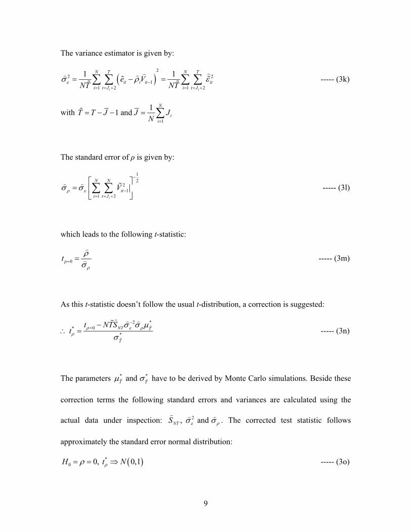
The variance estimator is given by:

( )2

2 21

1 2 1 2

1 1

i i

N T N T

it i it iti t J i t J

e VNT NTεσ ρ ε−

= = + = = +

= − =∑ ∑ ∑ ∑ ----- (3k)

with 1

11 and N

ii

T T J J JN =

= − − = ∑

The standard error of ρ is given by:

12

21

1 2i

N N

iti t J

Vρ εσ σ−

−= = +

⎡ ⎤= ⎢ ⎥

⎣ ⎦∑ ∑ ----- (3l)

which leads to the following t-statistic:

0ptρ

ρσ= = ----- (3m)

As this t-statistic doesn’t follow the usual t-distribution, a correction is suggested:

∴2 *

0**

NT T

T

t NTSt ρ ερ

ρσ σ μσ

−= −

= ----- (3n)

The parameters * and T T*μ σ have to be derived by Monte Carlo simulations. Beside these

correction terms the following standard errors and variances are calculated using the

actual data under inspection: 2, and NTS ε ρσ σ . The corrected test statistic follows

approximately the standard error normal distribution:

( )*0 0, 0,1H t Nρρ= = ⇒ ----- (3o)

9

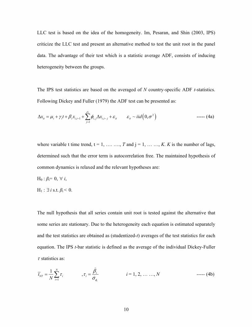
LLC test is based on the idea of the homogeneity. Im, Pesaran, and Shin (2003, IPS)

criticize the LLC test and present an alternative method to test the unit root in the panel

data. The advantage of their test which is a statistic average ADF, consists of inducing

heterogeneity between the groups.

The IPS test statistics are based on the averaged of N country-specific ADF t-statistics.

Following Dickey and Fuller (1979) the ADF test can be presented as:

, 1 , ,1

i

it i i i i t i j i t j itj

x t x xρ

μ γ β φ ε− −=

Δ = + + + Δ +∑ ( )2~ 0,it iidε σ ----- (4a)

where variable t time trend, t = 1, …. …., T and j = 1, … …, K. K is the number of lags,

determined such that the error term is autocorrelation free. The maintained hypothesis of

common dynamics is relaxed and the relevant hypotheses are:

H0 : βi= 0, ∀ i,

H1 : ∃ i s.t. βi < 0.

The null hypothesis that all series contain unit root is tested against the alternative that

some series are stationary. Due to the heterogeneity each equation is estimated separately

and the test statistics are obtained as (studentized-t) averages of the test statistics for each

equation. The IPS t-bar statistic is defined as the average of the individual Dickey-Fuller

τ statistics as:

1

1 N

NT ii

tN

τ=

= ∑ ,i

ii

φ

βτσ

= i = 1, 2, … …, N ----- (4b)

10

where iτ is the ADF test statistic for the ith country.

Assuming that the cross-sections are independent, Im, Pesaran and Shin (1997) propose

to use the following standardized t-bar statistic:

[ ]

( )

1

1

1 ( ,0)

1 ,0

N

NT iT ii

t N

it ii

N t E tN

Var tN

ρψ

ρ

=

=

⎧ ⎫−⎨ ⎬

⎩ ⎭=

⎡ ⎤⎣ ⎦

∑

∑ ----- (4c)

IPS suggest a fixed T, fixed N panel unit root test based on the ADF test statistics:

1

1 N

NT ii

tN

τ=

= ∑ ,i

ii

φ

βτσ

= i = 1, 2, … …, N ----- (4d)

where N is the number of panels, NTt is the average of the ADF test for each series across

the panel and values for E[tiT(pi,0)] and Var[tit(pi,0)] are obtained from the results of the

monte carlo simulation. The latter conjecture that the standardized t-bar statistic

Ψ t converge weakly to a standard normal distribution as N and T → ∞. Hence the panel

unit root inference can be conducted by comparing the obtained Ψt statistic to critical

values from the lower tail of the N(0,1) distribution. There are yet a number of

questionable aspects of this test.

First, despite the increase in power gained from the use of a panel, the test is still based

on the null that the series in question are unit root processes. Second, the null hypothesis

is that all of the series in the panel contain a unit root against the alternative that none do.

11

This assumption can be criticized by arguing that it is thus possible that outliers (in the

sense of a relatively high or low ADF for a particular series) have the potential to bias the

results and that the all-or-nothing approach is unattractive.

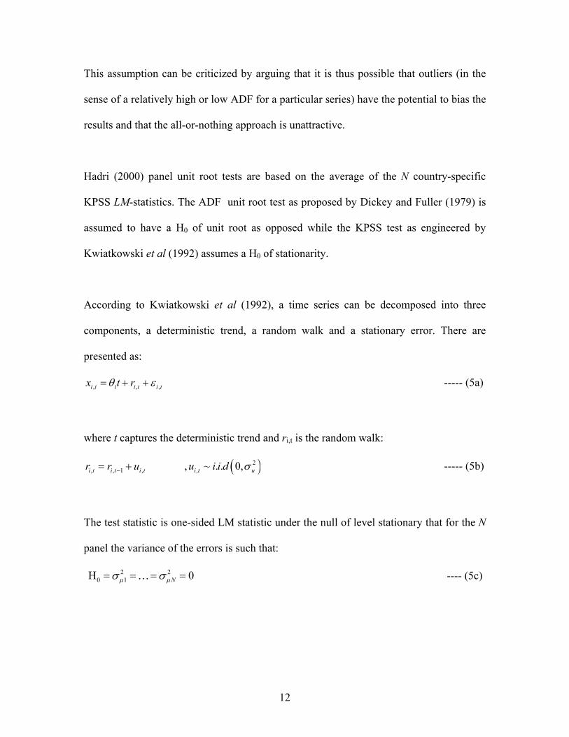
Hadri (2000) panel unit root tests are based on the average of the N country-specific

KPSS LM-statistics. The ADF unit root test as proposed by Dickey and Fuller (1979) is

assumed to have a H0 of unit root as opposed while the KPSS test as engineered by

Kwiatkowski et al (1992) assumes a H0 of stationarity.

According to Kwiatkowski et al (1992), a time series can be decomposed into three

components, a deterministic trend, a random walk and a stationary error. There are

presented as:

, ,i t i i t i tx t r ,θ ε= + + ----- (5a)

where t captures the deterministic trend and ri,t is the random walk:

, , 1i t i t i tr r u−= + , , ( )2, ~ . . 0,i t uu i i d σ ----- (5b)

The test statistic is one-sided LM statistic under the null of level stationary that for the N

panel the variance of the errors is such that:

---- (5c) 2 20 1H 0Nμ μσ σ= = = =…

12

against the alternative hypothesis that some This alternative allows for

heterogeneous

2 0.iμσ >

2iμσ across the cross-sections and includes the homogeneous alternative

( 2i

2μ μσ σ> for all i) as a special case. The LM test statistics is defined as:

( )2 2, ,2

1

1 T

i it

S lT ε εη

=

= ∑ iσ ----- (5d)

where T is the sample size, ( )2i lσ is estimated of the error variance, l, is the lag

truncation parameter and Si,t is the partial sums of the residuals, ,1

i

i t i jj

S ,ε=

=∑ . The lag

truncation is set to integer [4(T/100)1/4] to correct the estimate of the error variance. The

KPSS test makes a non-parametric correction of the estimate of the error variance such

that:

( )1

2 2, ,

1 1 1

1 2 1 21

T T

i i t it s t s

lT T l ,t i t sσ ε ε ε −

= = = +

−⎛ ⎞= + ⎜ ⎟+⎝ ⎠∑ ∑ ∑ ----- (5e)

The extension of the KPSS test for panel data has been performed by Hadri (2000). The

panel LM test statistic is defined as the mean of the individual test statistic under the null

of level stationary:

1

1 N

ii

LMNμ η

=

= ∑ ----- (5f)

13

The null hypothesis of level or trend stationary is tested against the alternative of unit

root in panel. Under the assumption that , ,E Ei t i tu ε⎡ ⎤ ⎡ ⎤ 0,= =⎣ ⎦ ⎣ ⎦ ui,t and εi,t are iid across i

and over t, the test statistic has the following limiting distribution:

( ) ( )0,1N LM

Z Nμ μμ

μ

ξ

ζ

−= ⇒ ----- (5g)

where represents weak convergence in distribution, ξ⇒ μ, ζμ are mean and variance of

the standard Brownian bridge The computed numerical values of ξ( )1

2

0

.V r dr∫ μ, ζμ are

1/6 and 1/45 for the level case and 1/15 and 11/6300 for the trend case respectively.

Karlsson and Löthgen (2000) suggest a caveat in using the IPS unit test which tends to

have high power in panels with large T and low power in panels with small T. As such,

researchers may draw wrong conclusions in claiming a whole panel is stationary even

though most individual series are non-stationary in case T is large. The reverse is true for

small T. On the contrary, the Hadri test performs well for panel data with short time

dimension (Barhoumi, 2005). A direct way of overcoming such shortcoming is to

reconcile the results of panel unit root tests.

In case the series are non-stationary and have the same integration order, two panel

cointegration tests will be considered. First, Nyblom and Harvey (2000, NH) postulates a

test of common trends where H0 is the stationarity of the series around a deterministic

trend, i.e. there exists k < n common trends (i.e. rank (Ση) = k), against the alternative of a

14

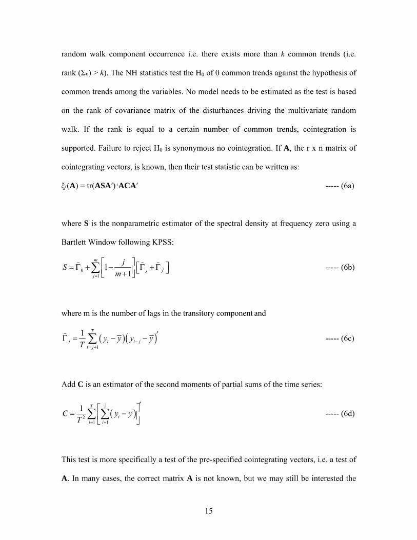
random walk component occurrence i.e. there exists more than k common trends (i.e.

rank (Ση) > k). The NH statistics test the H0 of 0 common trends against the hypothesis of

common trends among the variables. No model needs to be estimated as the test is based

on the rank of covariance matrix of the disturbances driving the multivariate random

walk. If the rank is equal to a certain number of common trends, cointegration is

supported. Failure to reject H0 is synonymous no cointegration. If A, the r x n matrix of

cointegrating vectors, is known, then their test statistic can be written as:

ξr(A) = tr(ASA′)-1ACA′ ----- (6a)

where S is the nonparametric estimator of the spectral density at frequency zero using a

Bartlett Window following KPSS:

01

11

m

j jj

jSm ′

=

⎡ ⎤ ⎡ ⎤= Γ + − Γ +Γ⎣ ⎦⎢ ⎥+⎣ ⎦∑ ----- (6b)

where m is the number of lags in the transitory component and

( )( )1

1 T

j t t jt j

y y y yT −

= +

′Γ = − −∑ ----- (6c)

Add C is an estimator of the second moments of partial sums of the time series:

( )21 1

1 T i

ti i

C yT = =

′⎡ ⎤= −⎢ ⎥⎣ ⎦∑ ∑ y ----- (6d)

This test is more specifically a test of the pre-specified cointegrating vectors, i.e. a test of

A. In many cases, the correct matrix A is not known, but we may still be interested the

15

testing for common trends. When A is not known, NH propose the following

modification to the above equation (6a):

( ) 1,

AASA ACAmink n trζ −⎡ ⎤′ ′= ⎣ ⎦ ----- (6e)

This allows A to be estimated for common trends. The univariate version of this test was

shown by Nyblom and Mäkeläinen (1983) to be the locally best invariant test of the null

hypothesis that , i.e. that the series is stationary. Note that this test can also be

interpreted as a one-sided Lagrange multiplier (LM) test. The test statistic in this case is:

2 0ησ =

ζ1 = C/S ----- (6f)

, since C and S will both be scalars when n = 1

NH also suggest a multivariate joint test for unit roots, a test for unit roots, a test for

. The test statistic in this final case is: 0η=∑

1n tr S Cζ −⎡ ⎤= ⎣ ⎦ ----- (6g)

The alternative is qη ε=∑ ∑ . The test maximizes the power against homogeneous

alternatives, but it is consistent against all non-null 'η∑ s. An advantage of the

parametric test is that is allows the inclusion of variables which may be correlated with

the variables of interest, thus they provide additional information, but they may not be

cointegrated with the variables of interest. But this is not possible in the NH world as the

vector A is required in order to work with a spectral density at frequency zero. From the

16

state-space representation of the correlated unobserved components model, Morley and

Sinclair (2005) derive the following variance-covariance matrix is obtained:

[ ]tt t

t

E η ηε

εη ε

ηη ε

ε⎡ ⎤⎛ ⎞⎡ ⎤

=⎜ ⎟ ⎢ ⎥⎢ ⎥⎣ ⎦⎝ ⎠ ⎣ ⎦

∑ ∑∑ ∑

----- (6h)

where ηit represents the innovation to the permanent component of series i in the model.

Hence, the submatrix of interest from the variance-covariance matrix is Ση. If this matrix

is of full rank then the series are all integrated but there does not exist any cointegration

vector. If it is of less than full rank, then either one or more of the series is stationary or

there exists at least one common trend.

The general correlated unobserved components model nests in this case the restricted

unobserved components model with at least one of the innovations to the permanent

component of one series is equal to a scale constant λ times the innovation to the

permanent component of another series. The distribution of the likelihood ratio test

statistic is once again nonstandard, but a Monte Carlo simulation can again be used to

establish appropriate confidence bands. The data for the Monte Carlo simulation can be

generated under the assumption that the restricted unobserved components model is the

true model. Consider the two-series example under the null of cointegration:

2 2

2 2 2η η

ηη η

σ λσλσ λ σ⎡ ⎤

= ⎢ ⎥⎢ ⎥⎣ ⎦

∑ ----- (6i)

17

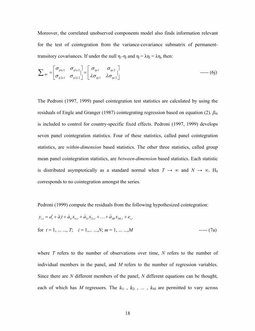
Moreover, the correlated unobserved components model also finds information relevant

for the test of cointegration from the variance-covariance submatrix of permanent-

transitory covariances. If under the null η1=η2 and η2 = λη1 = λη, then:

1 1 1 2 1 2

2 1 2 2 1 2

η ε η ε ηε ηεηε

η ε η ε ηε ηε

σ σ σ σσ σ λσ λσ⎡ ⎤ ⎡

= =⎢ ⎥ ⎢⎣ ⎦ ⎣

∑⎤⎥⎦

, ,

----- (6j)

The Pedroni (1997, 1999) panel cointegration test statistics are calculated by using the

residuals of Engle and Granger (1987) cointegrating regression based on equation (2). β0i

is included to control for country-specific fixed effects. Pedroni (1997, 1999) develops

seven panel cointegration statistics. Four of these statistics, called panel cointegration

statistics, are within-dimension based statistics. The other three statistics, called group

mean panel cointegration statistics, are between-dimension based statistics. Each statistic

is distributed asymptotically as a standard normal when T → ∞ and N → ∞. H0

corresponds to no cointegration amongst the series.

Pedroni (1999) compute the residuals from the following hypothesized cointegration:

, 1 1 , 2 2 ,i t t t t i t t i t Mt Mi t i ty a a t a x a x a x e′= + + + + + +…

for t = 1, ... ..., T; i = 1,... ...,N; m = 1, ... ...,M ----- (7a)

where T refers to the number of observations over time, N refers to the number of

individual members in the panel, and M refers to the number of regression variables.

Since there are N different members of the panel, N different equations can be thought,

each of which has M regressors. The â1i , â2i , ... , âMi are permitted to vary across

18

individual members of the panel. The parameter á is the member specific intercept, or

fixed effects parameter which of course is also allowed to vary across individual

members. In addition, deterministic time trends are included. These are specific to

individual members of the panel and are captured by the term äit, although it will also

often be the case that these äit terms are omitted.

Based on the residuals ei,t, Pedroni(1997, 1999) develops seven panel cointegration

statistics. Four of these statistics, called panel cointegration statistics, are within-

dimension based statistics which are constructed by summing both the numerator and the

denominator terms over the N dimension separately. The other three statistics, called

group mean panel cointegration statistics, are between-dimension based statistics and are

constructed by first dividing the numerator by the denominator prior to summing over the

N dimension. For the within-dimension statistics the test for the null of no cointegration

is implemented as a residual based test of the null hypothesis 0H : 1ia = for all i, versus

the alternative hypothesis 1H : 1ia a= < for all I, so that it presumes a common value

for . By contrast, for the between-dimension statistics the null of no cointegration is

implemented as a residual based test of the null hypothesis

ia a=

0H : 1ia = for all i, versus the

alternative hypothesis for all i, so that it does not presume a common value for

under the alternative hypothesis. Thus, the between-dimension based statistics

allow one to model an additional source of potential heterogeneity across individual

members of the panel. The asymptotic distributions of these panel cointegration statistics

are derived in Pedroni (1997). The panel cointegration statistics are shown in Box 1.

1H : 1ia <

ia a=

19

Box 1: Pedroni Panel Cointegration Statistics

1. Panel v-Statistics: ,

12 3 2 2 3 2 2 2

11 , 11 1

N T

N T

i i tVi t

T N Z T N L e−

−−

= =

⎛ ⎞≡ ⎜ ⎟⎝ ⎠∑∑

2. Panel ρ-Statistics: ( )1,

12 2 2 2

11 , 1 11 , 1 11 ,1 1 1 1

AN T

N T N T

i i t i i t i i t ii t i i

T N Z T N L e L e L e eρ −

−− − −

− −= = = =

⎛ ⎞≡ −⎜ ⎟⎝ ⎠∑∑ ∑∑

3. Panel pp-Statistics: ( ),

1 22 2 2 2 2

, 11 , 1 11 , 1 11 ,1 1 1 1

o AN T

N T N T

pp N T i i t i i t i i t ii t i i

Z L e L e L e e−

− − −− −

= = = =

⎛ ⎞≡ −⎜ ⎟⎝ ⎠

∑∑ ∑∑

4. Panel adf-Statistics: ,

1 2*2 2 2 2 2 * *

, 11 , 1 11 11 , ,1 1 1 1

s AN T

N T N T

adf N T i i t i i i t i ti t i i

Z L e L L e e−

− − −−

= = = =

⎛ ⎞≡ −⎜ ⎟⎝ ⎠

∑∑ ∑∑

5. Group ρ-Statistics: ( )1,

11 2 1 2 2

, 1 , 1 ,1 1 1

AN T

N T T

n i t i ti t t

TN Z TN e e e e−

−− −

− −= = =

⎛ ⎞i t i≡ −⎜ ⎟

⎝ ⎠∑ ∑ ∑

6. Group pp-Statistics: ( ),

1 21 2 1 2 2 2

, 1 , 1 ,1 1 1

o AN T

N T T

pp i i t i t i t ii t t

N Z N e e e e−

− −− −

= = =

⎛ ⎞≡ −⎜ ⎟⎝ ⎠

∑ ∑ ∑

7. Group adf-Statistics: ,

1 21 2 1 2 * *2 * *

, 1 , 1 ,1 1 1

AN T

N T T

adf i i t i t i ti t t

N Z N s e e e−

− −− −

= = =

⎛ ⎞≡ ⎜ ⎟⎝ ⎠

∑ ∑ ∑

i.e., , ,1 1

1 1 ,1

iK T

i i t i t ss t si

seT k

μ μ −= = +

⎛ ⎞= −⎜ ⎟−⎝ ⎠

∑ ∑ 2 2,

1

1 ,T

i it

sT tμ

=

≡ ∑ 2 2i is e= + o 2 ,i 2 2 2

, 11 i1

1 ,N

N T ii

LN

−

=

≡ ∑o o

*2 *2,

1

1 ,T

i i tiT

s μ=

≡ ∑ *2 *2,

1

1 ,N

N T ii

s sN =

≡ 2 211 , , ,

1 1 1

1 2 1 ,1

iKT T

i i t i t it s t si

sL ç ç çT T K t s−

= = = +

⎛ ⎞= + −⎜ ⎟+⎝ ⎠

∑ ∑ ∑∑

and where the residuals ,i tμ , *,i tμ and ,i tç are obtained from the following regressions:

, , 1 , ,i t i i t i te a e u−= + *, , 1 , ,

1A ,

iK

i t i i t i k i t k i tk

e a e u− −=

= + +∑ e a , , 1 , ,1

A AM

i t m mi t i tm

y b x ç=

= +∑

Source: Adopted from Pedroni (1999)

20

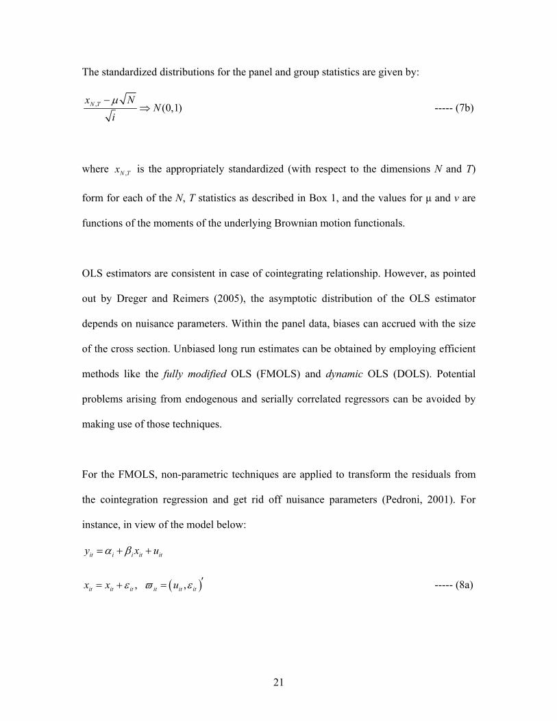
The standardized distributions for the panel and group statistics are given by:

, (0,1)N Tx NN

iμ−

⇒ ----- (7b)

where ,N Tx is the appropriately standardized (with respect to the dimensions N and T)

form for each of the N, T statistics as described in Box 1, and the values for μ and v are

functions of the moments of the underlying Brownian motion functionals.

OLS estimators are consistent in case of cointegrating relationship. However, as pointed

out by Dreger and Reimers (2005), the asymptotic distribution of the OLS estimator

depends on nuisance parameters. Within the panel data, biases can accrued with the size

of the cross section. Unbiased long run estimates can be obtained by employing efficient

methods like the fully modified OLS (FMOLS) and dynamic OLS (DOLS). Potential

problems arising from endogenous and serially correlated regressors can be avoided by

making use of those techniques.

For the FMOLS, non-parametric techniques are applied to transform the residuals from

the cointegration regression and get rid off nuisance parameters (Pedroni, 2001). For

instance, in view of the model below:

it i i it ity x uα β= + +

( ), ,it it it it it itx x uε ϖ ε ′= + = ----- (8a)

21

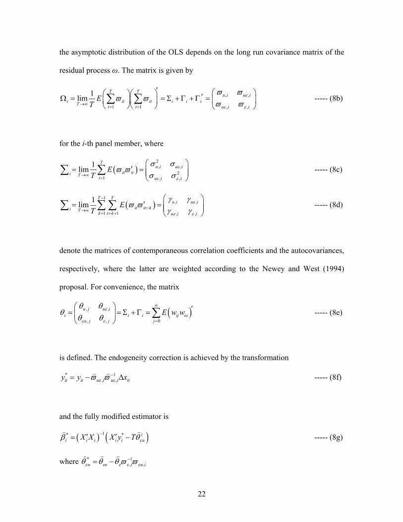
the asymptotic distribution of the OLS depends on the long run covariance matrix of the

residual process ω. The matrix is given by

, ,

1 1 , ,

1limT T

u i u ii it it i i iT t t u i i

ET

ε

ε ε

ϖ ϖϖ ϖ

ϖ ϖ→∞= =

′ ⎛ ⎞⎛ ⎞⎛ ⎞ ′Ω = = Σ +Γ +Γ = ⎜ ⎟⎜ ⎟⎜ ⎟⎝ ⎠⎝ ⎠ ⎝ ⎠∑ ∑ ----- (8b)

for the i-th panel member, where

( )2, ,

21 , ,

1limT

u i u iit iti T t u i i

ET

ε

ε ε

σ σϖ ϖ

σ σ→∞=

⎛ ⎞′= = ⎜ ⎟⎜ ⎟

⎝ ⎠∑ ∑ ----- (8c)

( )1

, ,

1 1 , ,

1limT T

u i u iit it ki T k t k u i i

ET

ε

ε ε

γ γϖ ϖ

γ γ

−

−→∞= = +

⎛ ⎞′= = ⎜ ⎟⎜ ⎟

⎝ ⎠∑ ∑ ∑ ----- (8d)

denote the matrices of contemporaneous correlation coefficients and the autocovariances,

respectively, where the latter are weighted according to the Newey and West (1994)

proposal. For convenience, the matrix

( ), ,

0, ,

u j u ii i i

ju j j

E w wε

ε ε

θ θθ

θ θ

∞

=

⎛ ⎞ij io

′= = Σ +Γ =⎜ ⎟⎝ ⎠

∑ ----- (8e)

is defined. The endogeneity correction is achieved by the transformation

* 1, ,it it u i u i ity y xε εϖ ϖ −= − Δ ----- (8f)

and the fully modified estimator is

( ) ( )1* * ii i i i iX X X y T εuβ θ−′ ′= − ----- (8g)

where * 1,u eu e i uε ε ,iεθ θ θ ϖ ϖ−= −

22

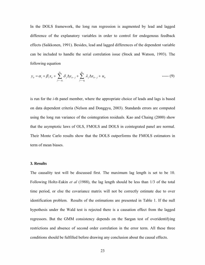
In the DOLS framework, the long run regression is augmented by lead and lagged

difference of the explanatory variables in order to control for endogenous feedback

effects (Saikkonen, 1991). Besides, lead and lagged differences of the dependent variable

can be included to handle the serial correlation issue (Stock and Watson, 1993). The

following equation

2 2

1 1

p q

it i i it j it j j it j itj p j q

y x y xα β δ λ− −=− =−

= + + Δ + Δ +∑ ∑ u ----- (9)

is run for the i-th panel member, where the appropriate choice of leads and lags is based

on data dependent criteria (Nelson and Donggyu, 2003). Standards errors are computed

using the long run variance of the cointegration residuals. Kao and Chaing (2000) show

that the asymptotic laws of OLS, FMOLS and DOLS in cointegrated panel are normal.

Their Monte Carlo results show that the DOLS outperforms the FMOLS estimators in

term of mean biases.

3. Results

The causality test will be discussed first. The maximum lag length is set to be 10.

Following Holtz-Eakin et al (1988), the lag length should be less than 1/3 of the total

time period, or else the covariance matrix will not be correctly estimate due to over

identification problem. Results of the estimations are presented in Table 1. If the null

hypothesis under the Wald test is rejected there is a causation effect from the lagged

regressors. But the GMM consistency depends on the Sargan test of overidentifying

restrictions and absence of second order correlation in the error term. All these three

conditions should be fulfilled before drawing any conclusion about the causal effects.

23

The Wald test for the null hypothesis that LGDP does not cause ELEC is rejected

throughout. Moreover, when the lag length is equal to two the pre-requite conditions for

the GMM consistency are fulfilled. As such there may to be an immediate impact of

LGDP on ELEC. However, it seems the impact of ELEC on LGDP might not be

instantaneously exerted. Causality conditions are achieved when the lag length is equal to

nine. This result suggests a possible long-run induced effect of electricity consumption on

income. This might be because African countries are lagging behind in terms of

technology to assist national production. As such better infrastructural conditions and

higher investment in R & D is required to boost economic growth. The relatively short

lag length of LGDP on ELEC indicates higher income has more immediate impact on

electricity consumption, which will in turn lead to higher demand in electricity in the

long run. However, because of multicollinearity problems among the lagged variables,

the causality test cannot distinguish whether LGDP has a positive or negative effect on

long run electric power consumption. Further analyses are required to answer this

question. As such we move on to unit and cointegration tests.

Results as shown in Table 2(a) and Table 2(b) regarding the order of integration of time

series for the ADF seem to match those of the KPSS. However mixed results are obtained

for the panel unit root tests as tabulated below. ELEC is I(0) as per LLC but I(1)

following IPS and Hadri. This most probably demonstrates the lack of power of the LLC

statistics as compared to more powerful test specifications. However, for order of

integration for LGDP seems to converge for all three tests. LLC and IPS clearly shows

that LGDP is I(1). For the Hadri test we can accept the null hypothesis for the first-

24

differenced data at 5% level of significance when controlling for serial correlation. Thus,

based on these tests, our series are apparently I(1).

As such we move on to apply the cointegration tests. In table 4(a), the NH test statistics

are reported under both the independent and identically distributed (iid) random walk

errors (NH-t) and the serially correlated residuals (NH adj-t) assumptions. The test is

calculated under two different specifications i.e. with fixed effects only while the second

with fixed effects plus time trends. Under the both specifications, H0 is rejected thus

revealing the existence of cointegrating vectors. The results for Pedroni’s (1997, 1999)

tests are presented in Table 4(b). Pedroni (1997) examined the small sample size and

properties of all these tests. In terms of power when T is small, the group-adf statistic

usually performs best, followed by the panel-adf statistic, whereas panel variance and the

group-ρ statistics do poorly. Our results tend to confirm Pedroni’s (1997) presumptions.

H0 is systematically rejected when referring to the group-adf and panel-adf statistics. As

maintained by both tests, cointegration between ELEC and LGDP is established. This

means that there is causality relationship between the two (Engle and Granger, 1987).

With this knowledge in mind, we move on to studying the income elasticities of electric

power consumption across various model specifications. As illustrated in Table 6, in

general, the Hausman’s (1978) specification test tends to favour the random-effects

models against the fixed-effects models. The coefficients in the random effects model are

assumed to constant across individuals and the variance unit-specific error term is zero.

However, the Breusch and Pagan’s (1980) Lagrangian multiplier test strongly rejects the

25

null hypothesis of Var(ν) = 0. In addition, in both fixed-effects and random-effects,

groupwise heteroskedasticity is detected by Greene’s (1993) methodology. Next, by

computing Wooldridge’s (2002) serial correlation test, the null of no first-order

autocorrelations in the residuals is not rejected. In case disturbances are not independent

and identically distributed Prais and Winsten (1954, PW) recommend a panel-corrected

standard error, which can correct for both correlated and heteroskedastic residuals.

However, given the lack of evidence of serial correlation we can estimate the PW model

assuming there is no first-order autocorrelation. We also conduct an error correction

mechanism (ECM) as popularized by Engle and Granger (1987) by using pooled data.

As shown in Table 5, the YEEPC seems to vary across models. In the PW models, the

YEEPC is less than one meaning a rather income inelastic demand for electric power

prevails in Africa. The above results seem to match those of the error correction

mechanism4 (ECM). The significance of the error term reinforces our knowledge about

the cointegrated relationship among the variables. Following Westerlund (2005), if the

null hypothesis of no error correction is rejected, then the null hypothesis of no

cointegration is also rejected. The small value signifies a moderate convergence speed

towards long run equilibrium prior to an exogenous shock. The short run elasticity of the

ECM is 0.39 as tabulated below.

The two-way causality as shown in Table 1 may create endogeneity and heterogeneity

problems which yield inconsistent estimates when using OLS to estimate the YEEPC. As

discussed above, to overcome such problems, efficient methods such as the FMOLS and 4 See Appendix 1 for derivation.

26

DOLS are required. These methods will allow us to compute long run asymptotic

unbiased estimates of the YEEPC. Table 6 reports Pedroni’s FMOLS and DOLS

estimates of the long run relationship between ELEC and LGDP. These estimates exclude

common time dummies given the lack of evidence that residuals are correlated across

countries. The FMOLS and DOLS group estimates are quite close to each other and

confirm a long run relationship between ELEC and GDP given the high significance of β.

These also confirm our a-priori expectation about the sign of the coefficient which is

positive and below unity. Electric power consumption is inelastic and considered as a

necessity in the long run. As shown in Table 6, a considerable degree of heterogeneity

appears to prevail in Africa even in the long run. For instance, when considering the least

biased estimator i.e. the DOLS estimates, the YEEPC ranges from -1.90 (Egypt) to 3.70

(Benin). In addition, with a few exceptions (Gabon, Nigeria, Senegal, South Africa,

Zimbabwe), the YEEPC is significantly less than zero, indicating evidence against the

ordinary electric power consumption-income relationship.

Finally, the YEEPC is modelled in relation to business cycles at an international level.

The measure of business cycle indicator is obtained as a cyclical component of the

Hodrick-Precott decomposition5 of natural logarithm of GDP of the individual countries.

A YEEPC series is constructed by running cross-sectional regressions over the period

1971-2002. Expect for the year 1972, all income elasticities were found to statistically

significant at conventional levels with their p-values which average around 0.02.

5 The smoothing parameter λ = 100 as per the frequency power rule of Ravn and Uhlig (2002) i.e. the number of periods per year divided by, raised to a power (which equals 2 following Hodrick and Prescott, 1997) and multiplied by 1600.

27

To evaluate the effects of our cluster-level dependent income elasticity variable, the use

of the population-averaged generalized estimating equations (GEE) approach as

pioneered by Liang and Zeger (1986), is arguably most appropriate. The GEE makes

efficient and appropriate use of the available data and neither sacrifices power by

collapsing observations over clusters nor overstates the amount of observations over the

amount of information contained in the data by ignoring dependencies among the

observations. It yields inferences for both individual- and cluster-level covariates that are

adjusted for intra-cluster as well as intra-individual correlation, in a manner that is

consistent with the way the study was designed. Put more plainly, the GEE allows the

number of repeat observations to vary among individual countries without affecting the

interpretation of the coefficients.

The estimates of the GEE are presented in Table 7. We make use of an unstructured intra-

individual correlation matrix R, which imposes no restrictions on the pairwise

correlations. This is recommended by Liang and Zeger (1986) when the number of

repeated observations per individual is not large, which is the case in our study. A

positive relationship between YEEPC and the cyclical component is found. This implies

a pro-cyclical pattern of electric power consumption where low levels of YEEPC are

associated with recession periods (i.e. electricity consumption is a necessity in periods of

recession) while high levels of income elasticities are associated with expansion periods

(i.e. electricity consumption becomes a luxury good in boom periods).

28

4. Conclusion

In this paper we have examined the non-stationarity and cointegration issues related to

electric power consumption and income for 16 African countries. Bi-directional causality

exists between ELEC and LGDP. Moreover both variables are found to be I(1) and

cointegrated. Panel FMOLS and DOLS long run estimates are positive and below unity.

Moreover, income elasticity of electric power consumption is found to be pro-cyclical.

Electricity consumption is a necessity in recession periods and luxury in boom periods.

Electricity demand studies have practical applications. The estimation of consistent and

stable income elasticity estimates can be of vital information for the African government

planners and private investors in regards to any privatization program for electric utility

sector. Greater access to electricity is bound to reduce the reliance on biomass which will

in turn lead to a decline in environmental degradation and sustain economic growth.

5. Reference

Al Mamun, K. A. and Nath, K. H., 2005, Export-led growth in Bangladesh: A time series

analysis, Applied Economics Letters, 12, pp. 361–364.

Arellano, M. and Bond, S., 1991, Some tests of specification for panel data: Monte

Carlo evidence and an application to employment equations, The Review of

Economic Studies, 58, pp. 277-297.

29

Barhoumi, K., 2005, Long run exchange rate pass-through into import prices in

developing countries: An homogeneous or heterogeneous phenomenon? Economics

Bulletin, 6, 14, pp. 1−12.

Bentzen, J. and Engsted, T., 1993, Short- and long-run elasticities in energy demand: a

cointegration approach, Energy Economics, 15, pp. 9-16.

Branch, R. E., 1993, Short run income elasticity of demand for residential electricity

using consumer expenditure survey data, Energy Journal, 14, 4, pp. 111-121.

Breusch, T. S. and Pagan, A. R., 1980, The Lagrange Multiplier test and its application to

model specification in econometrics, Review of Economic Studies, 47, pp. 239-254.

Cheng, S. B. and Lai, T. W. 1997, An investigation of co-integration and causality

between energy consumption and economic activity in Taiwan Province of China, Energy

Economics, 19, pp. 435-444.

Cheung, Y-W. and Lai, K. S. 1995, Lag order and critical values of the augmented

Dickey-Fuller test, Journal of Business and Economic Statistics, 13, 3, pp. 277-280.

Dickey, D.A, and Fuller, W. A., 1979, Distribution of the estimators for auto-regressive

time-series with a unit root. Journal of the American Statistical Association, 74, pp. 427-

431.

30

Deaton, A., 1997, The analysis of household surveys: A microeconomic approach to

development policy, Johns Hopkins University Press, Baltimore.

Dreger, C. and Reimers, H-E., 2005, Health care expenditures in OECD countries: A

panel unit root and cointegration analysis, IZA Discussion Paper Series No. 1469.

Engle, R. and Granger, C. W. J., 1987, Cointegration and error correction:

Representation, estimation, and testing, Econometrica, 55, pp. 251-276.

Fiebig, D. G., Seale J. J. and Theil, H., 1987, The demand for energy: evidence from a

cross-country demand system, Energy Economics, 9, pp. 149-153.

Ghosh, S. 2002, Electricity consumption and economic growth in India, Energy Policy

30, 2, pp. 125-129.

Gramlich, E. M., 1994, Infrastructure investment: A review essay. Journal of Economic

Literature 32, pp. 1176-1196.

Greene, W. H., 1993, Econometric analysis, Second Edition. New York: Macmillan.

Guttormsen, G. A., 2004, Causality between energy consumption and economic growth.

Discussion paper #D-24/2004.

31

Hausman, J., 1978, Specification tests in econometrics, Econometrica, 46, pp. 1251-

1271.

Hodrick, R. and Prescott, E., 1997, Post-war U.S. business cycles: An empirical

investigation, Journal of Money, Credit and Banking, 29, 1, pp. 1-16.

Holtedahl, P. and Joutz, F. L., 2004, Residential electricity demand in Taiwan, Energy

Economics, 26, pp. 201-224.

Holtz-Eakin, D., Newey W. and Rosen H., 1988, Estimating vector autoregressions with

panel data, Econometrica, 56, 6, pp. 1371-95.

Hunt, L. C. and Manning N., 1989, Energy price and income-elasticities of demand:

some estimates from the UK using the cointegration procedure, Scottish Journal of

Political Economy, 36, pp. 183-193.

Im, S. K., Pesaran, M. H. and Shin, Y., 2003, Testing for unit roots in heterogeneous

panels, Journal of Econometrics, 115, pp. 53-74.

Kao, C. and Chiang, M-H., 2000, On the estimation and the inference of a cointegrated

regression in panel data. In B. H. Baltagi, editor, Advances in Econometrics, 15, Elsevier

Press.

32

Kauffman, C., 2005, Energy and poverty in Africa, Policy Insights, 8, OECD.

Karlsson, S. and Löthgren, M., 2000, On the power and interpretation of panel unit root

tests, Economics Letters, 66, pp. 249-255.

Kraft, J. and Kraft A., 1978, On the relationship between energy and GNP”, Journal of

Energy and Development, 3, pp. 401-403.

Kouris, G., 1976, The determinants of energy demand in the EEC area, Energy Policy, 4,

pp. 343-355.

Kouris, G. 1983, Energy consumption and economic activity in industrialized economies

- a note, Energy Economics, 5, pp. 207-212.

Kwiatkowski, D., Phillips, P., Schmidt, P. and Shin, Y. (1992) Testing the null

hypothesis of stationarity against the alternative of unit root, Journal of Econometrics,

54, pp. 159-178.

Levin, A., Lin, C-F. and Chu, C-S. J., 2002, Unit root tests in panel data: Asymptotic and

finite sample properties, Journal of Econometrics, pp. 108, 1-24.

Liang K. Y. and Zeger S. L., 1986, Longitudinal data analysis using generalized linear

models, Biometrika, 73, pp.13–22.

33

Lise, W. and Van Montfort, K., 2005, Energy consumption and GDP in Turkey: Is there a

co-integration relationship? Working paper.

Liu, G., 2004, Estimating energy demand elasticities for OECD countries: A dynamic

panel data approach, Discussion paper, No. 373, Statistics Norway, Research

Department.

Morley, J. and Sinclaire, T. M., 2005, Testing for stationarity and cointegration in an

unobserved-components framework. Working paper.

Nelson, C. M. and Donggyu, S., 2003, Cointegration vector estimation by panel DOLS

and long-run money demand, Oxford Bulletin of Economics, 65, 5, pp. 665-680.

Newey, W. K., West, K. D., 1994, Automatic lag selection in covariance matrix

estimation, Review of Economic Studies, 61, pp. 631-653.

Nordhaus, W. D., 1977, The demand for energy: an international perspective. In

Nordhaus, W.D. (ed.) International Studies of the Demand for Energy, Amsterdam:

North-Holland.

Nyblom, J. and Harvey, A., 2000, Test of common stochastic trends, Econometric

Theory, 16, pp. 176-199.

34

Pedroni, P., 1997, Panel cointegration: Asymptotic and finite sample properties of pooled

time series tests with an application to the PPP hypothesis: New results, unpublished

manuscript, Indiana University.

Pedroni, P., 1999, Critical values for cointegration tests in heterogeneous panels with

multiple regressors, Oxford Bulletin of Economics and Statistics, 61, 4, pp. 653-670.

Pedroni, P., 2001, Purchasing power parity tests in cointegrated panels, Review of

Economics and Statistics, 83, pp. 727-731.

Prais, S. J. and Winsten, C. B., 1954, Trend estimators and serial correlation, Cowles

Commission, Discussion Paper No. 383.

Prosser, R. D. 1985, Demand elasticities in OECD countries: dynamic aspects, Energy

Economics, 7, pp. 9-1

Ravn, M. O. and Uhlig, H., 2002, On adjusting the Hodrick-Prescott filter for the

frequency of observations, Review of Economics and Statistics, 84, 371-375.

Saikkonen, P., 1991, Asymptotically efficient estimation of cointegration regression,

Econometric Theory, 7, pp. 1-21.

35

36

Shiu, A and Lam, P-L., 2004, Electricity consumption and economic growth in China,

Energy policy, 32, pp. 47-54.

Stock, J. H., Watson, M. W., 1993, A simple estimator of cointegration vectors in higher

order integrated systems; Econometrica, 61, pp. 783-820.

Yu, E. and Choi, J. 1985, The causal relationship between energy and GNP, an

international comparison, Journal of Energy and Development, 10, pp. 249–272.

Westerlund, J., 2005, Testing for error correction in panel data. Working Paper.

Wooldridge, J. M. (2002) Econometric analysis of cross section and panel data,

Cambridge, MA: MIT Press.

World Development Indicators, 2005, CD-ROM, The World Bank Group.

Table 1: Panel Causality Tests on ELEC and LGDP ELEC LGDP ELEC(-1) ELEC(-2) ELEC(-3) ELEC(-4) ELEC(-5) ELEC(-6) ELEC(-7) ELEC(-8) ELEC(-9) ELEC(-10)

0.761 (0.027)*

0.498 (0.040)* 0.266

(0.037)*

0.542 (0.048)*

0.187 (0.046)*

0.065 (0.040)

0.548 (0.049)*

0.160 (0.055)*

0.035 (0.048) 0.031

(0.041)

0.525 (0.049)*

0.186 (0.055)*-0.069 (0.055)-0.019 (0.049)0.125

(0.042)*

0.542 (0.052)*

0.174 (0.057)*

-0.079 (0.058) 0.017

(0.058) 0.104

(0.052)**-0.009 (0.044)

0.539 (0.052)*

0.176 (0.059)*-0.080 (0.059) 0.017

(0.060) 0.100

(0.060)‡

-0.009 (0.053) 0.001

(0.045)

0.542 (0.051)*

0.173 (0.058)*-0.092 (0.058) 0.025

(0.059) 0.092

(0.060) -0.048 (0.059) 0.029

(0.052) 0.007

(0.044)

0.586 (0.055)*0.142

(0.061)**-0.097 (0.061) 0.028

(0.063) 0.083 (0.063) -0.040 (0.063) 0.023 (0.060) 0.008 (0.054) -0.003 (0.046)

0.568 (0.056)*

0.166 (0.064)*-0.113

(0.062)‡

0.011 (0.064)0.088

(0.064)-0.048 (0.063)0.018

(0.063)0.008

(0.062)-0.05

(0.054)0.058

(0.046)

0.965 (0.017)*

1.215 (0.044)*

-0.277 (0.044)*

1.254 (0.048)* -0.318

(0.070)* 0.005

(0.046)

1.264 (0.047)*-0.366

(0.072)*0.023

(0.069)0.005

(0.045)

1.254 (0.049)*-0.357

(0.074)*(0.045) (0.073)-0.046 (0.069)0.038

(0.044)

1.223 (0.047)*-0.400

(0.072)*0.133

(0.070)‡

-0.114 (0.068)‡

0.116 (0.063)‡

-0.060 (0.041)

1.276 (0.051)*-0.429

(0.077)* 0.158

(0.077)**-0.172

(0.073)**0.143

(0.070)**-0.010 (0.066) -0.056 (0.042)

1.217 (0.050)*

-0.283 (0.078)*

0.088 (0.075) -0.155

(0.072)**0.102

(0.069) -0.017 (0.066) 0.037

(0.062) -0.074

(0.040)‡

1.240 (0.054)* -0.304

(0.082)* 0.050

(0.081) -0.130

(0.077)‡

0.078 (0.074) 0.008

(0.071) -0.003 (0.067) -0.003 (0.063) -0.050 (0.041)

1.218 (0.054)* -0.258

(0.084)* 0.064

(0.082) -0.218

(0.080)* 0.146

(0.075)‡

-0.045 (0.073) 0.025

(0.069) -0.023 (0.066) 0.013

(0.062) -0.060 (0.041)

LGDP(-1) LGDP(-2) LGDP(-3) LGDP(-4) LGDP(-5) LGDP(-6) LGDP(-7) LGDP(-8) LGDP(-9) LGDP(-10)

0.293

(0.060)*

0.285

(0.050)* 0.005

(0.124)

0.260

(0.054)* 0.105

(0.172) -0.118 (0.132)

0.298

(0.057)* -0.145 (0.219) 0.303

(0.284) -0.234

(0.134)‡

0.344 (0.062)* 0.013 (0.263)* 0.111 (0.472) -0.003 (0.401) -0.058 (0.132)

0.349

(0.069)*-0.311

(0.324) 1.053

(0.723) -1.376

(0.878) 0.892

(0.540)‡

-0.247 (0.136) ‡

0.344

(0.076)*-0.260 (0.382) 1.114

(1.028) -1.592 (1.593) 1.169

(1.419) -0.417 (0.679) 0.040

(0.137)

0.378

(0.082)*-0.270 (0.433) 1.107

(1.372) -2.164 (2.579) 2.121

(2.971) -1.197 (2.070) 0.376

(0.805) -0.064 (0.136)

0.337

(0.094)*-0.043 (0.527) 0.262

(1.900) -0.312 (4.186) -0.627 (5.879) 1.353

(5.329) -1.092 (3.033) 0.418

(0.990) -0.070 (0.143)

0.363

(0.106)*-0.138 (0.613)1.029

(2.468)-2.874 (6.219)4.044

(10.272)-4.213

(11.413)3.376

(8.500)-1.906 (4.084)0.639

(1.149)-0.096 (0.145)

-0.017

(0.007)**

0.0004 (0.009) .0165

(0.014)

-0.004 (0.010) -0.026 (0.025) 0.027

(0.015)‡

0.012

(0.010) 0.031

(0.033) -0.102

(0.038)*0.048

(0.014)*

0.012

(0.011)-0.0001 (0.040)-0.019 (0.068)-0.031 (0.051)0.027

(0.015)‡

0.036

(0.011)*-0.046 (0.043)0.051

(0.100)-0.082 (0.110)0.052

(0.061)-0.009

(0.014)

0.027

(0.012)**-0.036 (0.051) 0.063

(0.143) -0.122 (0.216) 0.094

(0.180) -0.023 (0.078) 0.001

(0.014)

0.019

(0.013) -0.007 (0.054) 0.060

(0.181) -0.179 (0.339) 0.168

(0.373) -0.059 (0.243) 0.002

(0.087) 0.003

(0.013)

0.035

(0.014)**-0.050 (0.062) 0.045

(0.235) 0.009

(0.528) -0.176 (0.723) 0.265

(0.624) -0.170 (0.334) 0.050

(0.101) -0.005 (0.013)

0.047

(0.015)* -0.136

(0.068)** 0.372

(0.286) -0.752 (0.745) 0.987

(1.220) -0.931 (1.313) 0.653

(0.933) -0.317 (0.424) 0.091

(0.112) -0.011 (0.013)

No. Observations Sargan Test AR(1) AR(2)

Wald Tests: χ2 -test, LGDP lags

χ2 -test, ELEC lags

480 1.000

0.000* 0.039**

23.76 [0.000]*

464 0.756 0.000* 0.483

36.40 [0.000]*

448 0.967

0.000* 0.018**

32.23 [0.000]*

432 0.989

0.000* 0.010*

35.18 [0.000]*

416 0.992 0.000*0.988

44.12 [0.000]*

400 0.999 0.000*0.388

33.60 [0.000]*

384 0.997

0.000* 0.794

29.76 [0.000]*

368 0.990 0.000* 0.488

33.39 [0.000]*

352 1.000 0.000*

0.035**

30.69 [0.000]*

336 0.999 0.000* 0.310

31.70 [0.000]*

480 0.219 0.000*

0.027**

5.47 [0.019]**

464 1.000 0.000* 0.502

1.50 [0.473]

448 1.000

0.000* 0.141

4.06 [0.222]

432 1.000 0.000 0.001*

14.95 [0.005]*

416 1.000 0.000*

0.031**

24.43 [0.000]*

400 0.998

0.000* 0.019**

19.48 [0.000]*

384 1.000 0.000* 0.006*

12.22 [0.094]‡

368 0.997

0.000* 0.345

9.99 [0.2658]

352 1.000 0.000* 0.126

14.88 [0.094]‡

336 1.000 0.000* 0.211

19.70 [0.032]**

Source: Computed. The p-value for the Sargan test, AR(1) and AR(2) serial correlation tests are shown. *, ** and ‡ denote 1%, 5% and 10% significance level respectively. The standard errors are given in parentheses while the p-values are in square brackets.

37

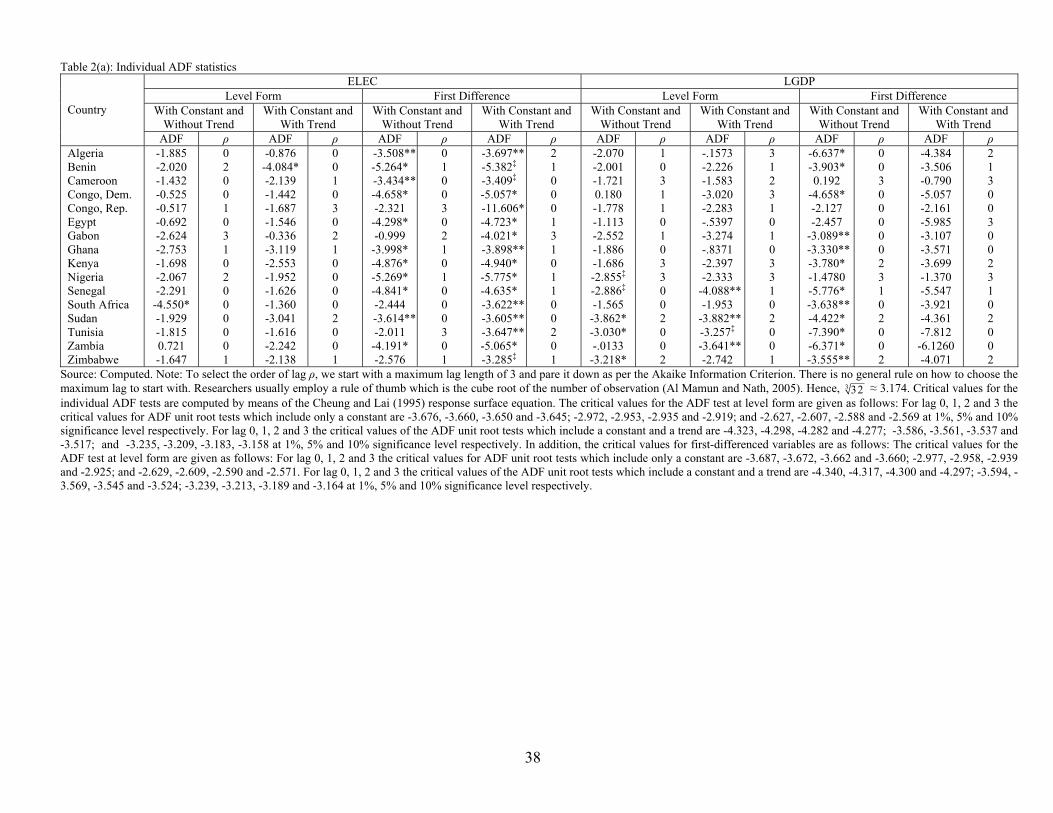
Table 2(a): Individual ADF statistics ELEC LGDP

Level Form First Difference Level Form First Difference With Constant and

Without Trend With Constant and

With Trend With Constant and

Without Trend With Constant and

With Trend With Constant and

Without Trend With Constant and

With Trend With Constant and

Without Trend With Constant and

With Trend Country

ADF ρ ADF ρ ADF ρ ADF ρ ADF ρ ADF ρ ADF ρ ADF ρ Algeria Benin Cameroon Congo, Dem. Congo, Rep. Egypt Gabon Ghana Kenya Nigeria Senegal South Africa Sudan Tunisia Zambia Zimbabwe

-1.885 -2.020 -1.432 -0.525 -0.517 -0.692 -2.624 -2.753 -1.698 -2.067 -2.291

-4.550* -1.929 -1.815 0.721 -1.647

0 2 0 0 1 0 3 1 0 2 0 0 0 0 0 1

-0.876 -4.084* -2.139 -1.442 -1.687 -1.546 -0.336 -3.119 -2.553 -1.952 -1.626 -1.360 -3.041 -1.616 -2.242 -2.138

0 0 1 0 3 0 2 1 0 0 0 0 2 0 0 1

-3.508**-5.264* -3.434**-4.658* -2.321

-4.298* -0.999

-3.998* -4.876* -5.269* -4.841* -2.444 -3.614**-2.011

-4.191* -2.576

0 1 0 0 3 0 2 1 0 1 0 0 0 3 0 1

-3.697**-5.382‡

-3.409‡

-5.057* -11.606*-4.723* -4.021* -3.898**-4.940* -5.775* -4.635* -3.622**-3.605**-3.647**-5.065* -3.285‡

2 1 0 0 0 1 3 1 0 1 1 0 0 2 0 1

-2.070 -2.001 -1.721 0.180 -1.778 -1.113 -2.552 -1.886 -1.686 -2.855‡

-2.886‡

-1.565 -3.862* -3.030* -.0133

-3.218*

1 0 3 1 1 0 1 0 3 3 0 0 2 0 0 2

-.1573 -2.226 -1.583 -3.020 -2.283 -.5397 -3.274 -.8371 -2.397 -2.333

-4.088**-1.953

-3.882**-3.257‡

-3.641**-2.742

3 1 2 3 1 0 1 0 3 3 1 0 2 0 0 1

-6.637* -3.903* 0.192

-4.658* -2.127 -2.457

-3.089**-3.330**-3.780* -1.4780 -5.776* -3.638**-4.422* -7.390* -6.371* -3.555**

0 0 3 0 0 0 0 0 2 3 1 0 2 0 0 2

-4.384 -3.506 -0.790 -5.057 -2.161 -5.985 -3.107 -3.571 -3.699 -1.370 -5.547 -3.921 -4.361 -7.812

-6.1260 -4.071

2 1 3 0 0 3 0 0 2 3 1 0 2 0 0 2

Source: Computed. Note: To select the order of lag ρ, we start with a maximum lag length of 3 and pare it down as per the Akaike Information Criterion. There is no general rule on how to choose the maximum lag to start with. Researchers usually employ a rule of thumb which is the cube root of the number of observation (Al Mamun and Nath, 2005). Hence, 3 32 ≈ 3.174. Critical values for the individual ADF tests are computed by means of the Cheung and Lai (1995) response surface equation. The critical values for the ADF test at level form are given as follows: For lag 0, 1, 2 and 3 the critical values for ADF unit root tests which include only a constant are -3.676, -3.660, -3.650 and -3.645; -2.972, -2.953, -2.935 and -2.919; and -2.627, -2.607, -2.588 and -2.569 at 1%, 5% and 10% significance level respectively. For lag 0, 1, 2 and 3 the critical values of the ADF unit root tests which include a constant and a trend are -4.323, -4.298, -4.282 and -4.277; -3.586, -3.561, -3.537 and -3.517; and -3.235, -3.209, -3.183, -3.158 at 1%, 5% and 10% significance level respectively. In addition, the critical values for first-differenced variables are as follows: The critical values for the ADF test at level form are given as follows: For lag 0, 1, 2 and 3 the critical values for ADF unit root tests which include only a constant are -3.687, -3.672, -3.662 and -3.660; -2.977, -2.958, -2.939 and -2.925; and -2.629, -2.609, -2.590 and -2.571. For lag 0, 1, 2 and 3 the critical values of the ADF unit root tests which include a constant and a trend are -4.340, -4.317, -4.300 and -4.297; -3.594, -3.569, -3.545 and -3.524; -3.239, -3.213, -3.189 and -3.164 at 1%, 5% and 10% significance level respectively.

38

39

Table 2(b): Individual KPSS η-statistics ELEC LGDP

Level Form First Difference Level Form First Difference Country ηm ρ ηt ρ ηm ρ ηt ρ ηm ρ ηt ρ ηm ρ ηt ρ

Algeria Benin Cameroon Congo, Dem. Congo, Rep. Egypt Gabon Ghana Kenya Nigeria Senegal South Africa Sudan Tunisia Zambia Zimbabwe

1.220* 1.660* 0.331

1.140* 0.481** 1.240* 0.750* 0.173

1.180* 0.852* 1.140* 1.090* 1.080* 1.260* 1.210* 0.308

2 2 2 2 2 2 2 2 2 2 2 2 2 2 2 2

0.310* 0.133‡

0.249* 0.176** 0.250* 0.296* 0.281* 0.104

0.240* 0.296* 0.158‡

0.294* 0.061

0.275* 0.233* 0.129‡

2 2 2 2 2 2 2 2 2 2 2 2 2 2 2 2

0.647* 0.142 0.213 0.080 0.213 0.263 0.283 0.040 0.387‡

0.510‡

0.158 0.680** 0.075 0.392‡

0.262 0.300

2 2 2 2 2 2 2 2 2 2 2 2 1 2 1 3

0.080 0.111 0.050 0.069 0.105 0.090 0.086 0.039 0.041 0.047 0.154‡

0.124‡

0.074 0.090 0.112 0.142‡

2 2 2 2 2 2 2 2 2 2 2 2 1 4 2 2

0.322 0.675** 0.268

1.200* 0.342

1.220* 0.356‡

0.353‡

0.743* 0.604** 0.255

0.860* 0.760* 1.240* 1.240* 0.115

2 2 2 2 2 2 2 2 2 2 2 2 1 4 2 2

0.257* 0.136** 0.264* 0.257* 0.262* 0.266* 0.080

0.305* 0.224* 0.198** 0.178** 0.134‡

0.179** 0.156‡

0.144‡

0.073

2 2 2 2 2 2 2 2 2 2 2 2 1 4 2 2

0.539** 0.158 0.330 0.267 0.262 0.222 0.145

0.548** 0.354 0.092 0.150 0.080 0.119 0.259 0.155 0.103

2 2 2 2 2 2 2 2 2 5 2 2 2 2 2 2

0.226* 0.082 0.151‡

0.086 0.068 0.074 0.086 0.049 0.049 0.076 0.049 0.075 0.054

0.195** 0.119‡

0.074

2 2 2 2 2 2 2 2 2 5 2 2 2 2 2 2

Source: Computed. Note: ηm and ηt are the level and trend stationarity cases respectively. The 1%, 5% and 10% critical values are 0.739, 0.463 and 0.347 for level stationarity and 0.216, 0.176 and 0.119 for tend stationarity correspondingly. Theses critical values are given by Kwiatkowski et al (1992). The order of lag ρ is determined by the automatic bandwidth selection procedure as proposed by Newey and West (1994). The test’s denominator is computed by employing the Quadratic Spectral kernel function.

Table 3(a): LLC Panel Unit Root Test statistics Level Form First Difference

Variable Deterministics t-value t* t-value t* Constant -4.174 -2.020 [0.022]** -21.303 -13.789 [0.000]* ELEC Constant + Trend -10.614 -4.355 [0.000]* -25.086 -14.147 [0.000]* Constant -4.216 -1.163 [0.122] -18.194 -12.321 [0.000]* LGDP Constant + Trend -8.908 -1.862 [0.031]** -18.822 -9.077 [0.000]*

Source: Computed. Note: The LLC test can be viewed as a pooled Dickey-Fuller test, or an Augmented Dickey-Fuller (ADF) test when lags are included, with the null hypothesis that of non-stationarity (I(1) behavior). The lag lengths for the panel test are based on those employed in the univariate ADF test. These statistics are distributed as standard normal as both N and T grow large. Assuming no cross-country correlation and T is the same for all country, the normalized t* test statistic is computed by using the t-value statistics. After transformation by factors provided by LLC, the t* tests is distributed standard normal under the null hypothesis of non-stationarity. Hence, it is compared the 1%, 5% and 10% significance levels with critical values of -2.326, -1.645 and -1.282 correspondingly. The p-values are in square brackets. Table 3(b): IPS Panel Unit Root Test statistics

Level Form First Difference Variable Data Deterministics t-bar Ψt t-bar Ψt

Constant -2.173* -2.972 [0.001]* -4.628* -13.991 [0.000]* Raw Constant + Trend -2.546** -1.866 [0.031]** -5.323* -15.344 [0.000]* Constant -1.586 -0.328 [0.371] -5.355* -17.257 [0.000]* ELEC

Demeaned Constant + Trend -2.704* -2.636 [0.001]* -5.999* -18.629 [0.000]* Constant -1.915** -1.825 [0.034]** -4.449* -13.203 [0.000]* Raw Constant + Trend -2.231 -0.370 [0.356] -4.186* -9.835 [0.000]* Constant -1.728 -0.987 [0.164] -4.445* -13.182 [0.000]* LGDP

Demeaned Constant + Trend -2.253 -0.476 [0.317] -4.563* -11.657 [0.000]* Source: Computed. Note: The IPS test statistics are computed as the average ADF statistics across the sample. The lag lengths for the panel test are based on those employed in the univariate ADF test. These statistics are distributed as standard normal as both N and T grow large. t-bar is the panel test based on the ADF statistics. Critical values for the t-bar statistics without trend at 1%, 5% and 10% significance levels are -1.980, -1.850 and -1.780 while with inclusion of a time trend, the critical values are-2.590, -2.480 and -2.410 respectively. Assuming no cross-country correlation and T is the same for all country, the normalized Ψt test statistic is computed by using the t-bar statistics. The Ψt- tests for H0 of joint non-stationarity and is compared to the 1%, 5% and 10% significance levels with critical values of -2.326, -1.645 and -1.282 correspondingly. Table 3(c): Hadri Panel Unit Root Test Statistics

Level Form First Difference Homoskedastic Disturbances

Heteroskedastic Disturbances

Controlling for Serial Dependence in Errors

Homoskedastic Disturbances

Heteroskedastic Disturbances

Controlling for Serial Dependence in Errors Variables

Zμ Zt Zμ Zt Zμ Zt Zμ Zt Zμ Zt Zμ Zt

ELEC 57.007 [0.000]*

35.528 [0.000]*

50.847 [0.000]*

34.889 [0.000]*

20.371 [0.000]*

14.194 [0.000]*

-1.856 [0.968]

-3.129 [0.991]

3.268 [0.001]*

-0.390 [0.6519]

0.029 [0.488]

-0.008 [0.503]

LGDP 56.655 [0.000]*

39.226 [0.000]*

35.682 [0.000]*

31.982 [0.000]*

19.159 [0.000]*

13.339 [0.000]*

3.487 [0.000]*

4.225 [0.000]*

3.894 [0.000]*

3.807 [0.000]*

1.544 [0.061]‡

2.478 [0.007]*

Source: Computed. Note: Zμ and Zt denote the statistics without and with a deterministic trend respectively.

40

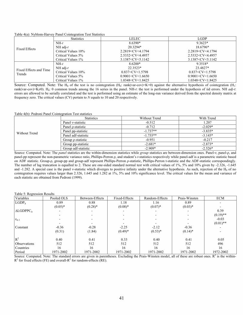
Table 4(a): Nyblom-Harvey Panel Cointegration Test Statistics Statistics LELEC LGDP

Fixed Effects

NH-t NH adj-t Critical Values 10% Critical Values 5% Critical Values 1%

8.6390* 20.3294*

2.2819<CV<4.1794 2.5332<CV<4.4957 3.1387<CV<5.1142

9.3623* 18.6796*

2.2819<CV<4.1794 2.5332<CV<4.4957 3.1387<CV<5.1142

Fixed Effects and Time Trends

NH-t NH adj-t Critical Values 10% Critical Values 5% Critical Values 1%

8.6200* 22.3523*

0.837<CV<1.5798 0.9001<CV<1.6650 1.0348<CV<1.8425

9.3518* 23.4827*

0.837<CV<1.5798 0.9001<CV<1.6650 1.0348<CV<1.8425

Source: Computed. Note: The H0 of the test is no cointegration (H0: rank(var-cov)=K=0) against the alternative hypothesis of cointegration (H1: rank(var-cov)=K≠0). H0: 0 common trends among the 16 series in the panel. NH-t: the test is performed under the hypothesis of iid errors. NH adj-t: errors are allowed to be serially correlated and the test is performed using an estimate of the long-run variance derived from the spectral density matrix at frequency zero. The critical values (CV) pertain to N equals to 10 and 20 respectively.

Table 4(b): Pedroni Panel Cointegration Test statistics Statistics Without Trend With Trend

Panel ν-statistic -0.512 1.207 Panel ρ-statistic -0.712 -2.029* Panel pp-statistic -1.737** -3.835* Panel adf-statistic -1.755** -3.145* Group ρ-statistic -0.951 -0.217 Group pp-statistic -2.681* -2.873*

Without Trend

Group adf-statistic -2.909* -2.526* Source: Computed. Note: The panel statistics are the within-dimension statistics while group statistics are between-dimension ones. Panel-ν, panel-ρ, and panel-pp represent the non-parametric variance ratio, Phillips-Perron ρ, and student’s t-statistics respectively while panel-adf is a parametric statistic based on ADF statistic. Group-ρ, group-pp and group-adf represent Phillips-Perron ρ-statistic, Phillips-Perron t-statistic and the ADF-statistic correspondingly. The number of lag truncation is equalled to 2. These are one-sided standard normal test with critical values of 1%, 5% and 10% given by -2.326, -1.645 and -1.282. A special case is the panel ν-statistic which diverges to positive infinity under the alternative hypothesis. As such, rejection of the H0 of no cointegration requires values larger than 2.326, 1.645 and 1.282 at 1%, 5% and 10% significance level. The critical values for the mean and variance of each statistic are obtained from Pedroni (1999). Table 5: Regression Results Variables Pooled OLS Between-Effects Fixed-Effects Random-Effects Prais-Winsten ECM LGDPit

∆LGDPPCit

εit-1

Constant

R2

Observations Countries Period

0.89 (0.05)*

- - - -

-0.36 (0.31)

0.40 512 16

1971-2002

0.88 (0.28)*

- - - -

-0.28 (1.84)

0.41 512 16

1971-2002

1.18 (0.08)*

- - - -

-2.25 (0.49)*

0.33 512 16

1971-2002

1.16 (0.07)*

- - - -

-2.12 (0.53)*

0.40 512 16

1971-2002

0.89 (0.03)*

- - - -

-0.36 (0.14)*

0.41 512 16

1971-2002

- -

0.39 (0.19)**

-0.03 (0.01)**

- -

0.05 496 16

1972-2002 Source: Computed. Note: The standard errors are given in parentheses. Excluding the Prais-Winsten model, all of these are robust ones. R2 is the within-R2 for fixed effects (FE) and overall-R2 for random-effects (RE).

41

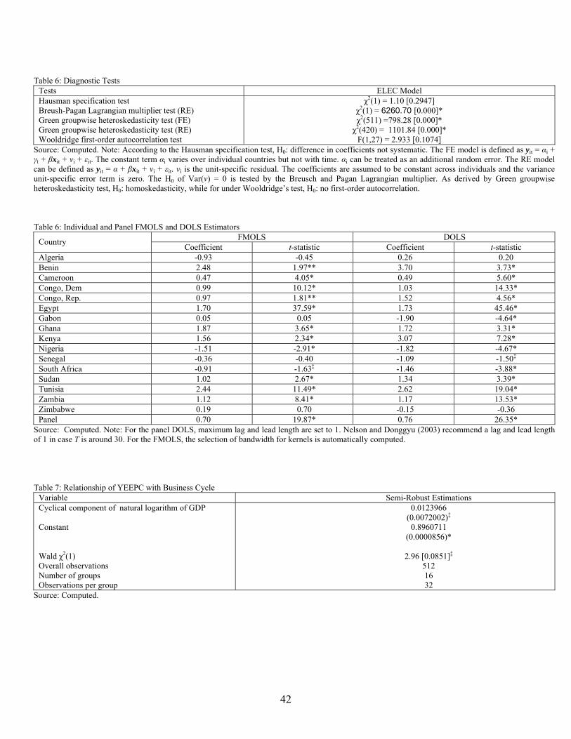
Table 6: Diagnostic Tests Tests ELEC Model Hausman specification test Breush-Pagan Lagrangian multiplier test (RE) Green groupwise heteroskedasticity test (FE) Green groupwise heteroskedasticity test (RE) Wooldridge first-order autocorrelation test

χ2(1) = 1.10 [0.2947] χ2(1) = 6260.70 [0.000]* χ2(511) =798.28 [0.000]* χ2(420) = 1101.84 [0.000]*

F(1,27) = 2.933 [0.1074] Source: Computed. Note: According to the Hausman specification test, H0: difference in coefficients not systematic. The FE model is defined as yit = αi + γt + βxit + νi + εit. The constant term αi varies over individual countries but not with time. αi can be treated as an additional random error. The RE model can be defined as yit = α + βxit + νi + εit. νi is the unit-specific residual. The coefficients are assumed to be constant across individuals and the variance unit-specific error term is zero. The H0 of Var(ν) = 0 is tested by the Breusch and Pagan Lagrangian multiplier. As derived by Green groupwise heteroskedasticity test, H0: homoskedasticity, while for under Wooldridge’s test, H0: no first-order autocorrelation. Table 6: Individual and Panel FMOLS and DOLS Estimators

FMOLS DOLS Country Coefficient t-statistic Coefficient t-statistic Algeria -0.93 -0.45 0.26 0.20 Benin 2.48 1.97** 3.70 3.73* Cameroon 0.47 4.05* 0.49 5.60* Congo, Dem 0.99 10.12* 1.03 14.33* Congo, Rep. 0.97 1.81** 1.52 4.56* Egypt 1.70 37.59* 1.73 45.46* Gabon 0.05 0.05 -1.90 -4.64* Ghana 1.87 3.65* 1.72 3.31* Kenya 1.56 2.34* 3.07 7.28* Nigeria -1.51 -2.91* -1.82 -4.67* Senegal -0.36 -0.40 -1.09 -1.50‡

South Africa -0.91 -1.63‡ -1.46 -3.88* Sudan 1.02 2.67* 1.34 3.39* Tunisia 2.44 11.49* 2.62 19.04* Zambia 1.12 8.41* 1.17 13.53* Zimbabwe 0.19 0.70 -0.15 -0.36 Panel 0.70 19.87* 0.76 26.35*

Source: Computed. Note: For the panel DOLS, maximum lag and lead length are set to 1. Nelson and Donggyu (2003) recommend a lag and lead length of 1 in case T is around 30. For the FMOLS, the selection of bandwidth for kernels is automatically computed. Table 7: Relationship of YEEPC with Business Cycle

Variable Semi-Robust Estimations Cyclical component of natural logarithm of GDP Constant Wald χ2(1) Overall observations Number of groups Observations per group

0.0123966 (0.0072002)‡

0.8960711 (0.0000856)*

2.96 [0.0851]‡

512 16 32

Source: Computed.

42

Appendix 1: Derivation of the First-Order Panel ECM model

Consider the equation below:

ELECit = β0 + β1LGDPit + εit ----- (1)

To derive the long run equilibrium dynamics we re-write equation (1) as follows, while assuming ELECit and LGDPit are non-

stationary, integrated of the same order and εit is white-noise:

ELECit = β0 + β1LGDPit + β2LGDPit-1 + β3ELECit-1 + εit

Subtracting ELECit-1 on both sides:

ELECit – ELECit-1= β0 + β1LGDPit + β2LGDPit-1+ β3ELECit-1 - ELECit-1 + εit

ΔELECit = β0 + β1LGDPit + β2LGDPit-1+ (β3 - 1)ELECit-1 + εit

Repametrizing the above equation:

ΔELECit = β0 + β1LGDPit - β1LGDPit-1 + β1LGDPit-1+ β2LGDPit-1 + (β3 - 1)ELECit-1 + εit

ΔELECit = β0 + β1ΔLGDPit + (β1 + β2)LGDPit-1 + (β3 - 1)ELECit-1 + εit

ΔELECit = β1ΔLGDPt + (β1 + β2)LGDPit-1 + β0 + (β3 - 1)ELECit-1 + εit

ΔELECit = β1ΔLGDPit - (1 – β3)0 1 2

it-1 it-13 3

β β +βELEC - - LGDP

1 - β 1 - β

⎡ ⎤⎢ ⎥⎣ ⎦

+ εit

ΔELECit = β1ΔLGDPit – λ[ ] it-1 0 1 it-1ELEC - λ - λ LGDP + εit

∴ ΔELECit = β1ΔLGDPit - λεit,-1 + εit,

The disequilibrium error εit,-1 = and is assumed to be I(0). λ measures the speed of adjustment towards the

long run equilibrium.

it-1 0 1 it-1ELEC - λ - λ LGDP

43