incentives in the public sector: some preliminary evidence ... · incentives in the public sector:...
TRANSCRIPT

CMPO Working Paper Series No. 03/080
CMPO is funded by the Leverhulme Trust.
Incentives in the Public Sector: Some Preliminary Evidence from a
UK Government Agency
Simon Burgess University of Bristol, CMPO and CEPR
Carol Propper
University of Bristol, CMPO and CEPR
Marisa Ratto CMPO
Emma Tominey
CMPO
July 2003
Abstract This paper evaluates the impact of a team-based incentive scheme piloted in the public sector agency, Jobcentre Plus. The way the scheme has been designed raises many questions for which theory makes predictions. We test these predictions against our data. We find that team size affects the impact of the incentive scheme upon performance. Moreover, while the measure of quantity increased in incentivised areas, no improvement was found for the two quality measures. This may reflect concerns related to multi-tasking issues, or may reflect the small sample size available for the quality analysis. Finally, the data suggests that employees participating in the incentive scheme aim to exert a level of effort to ensure the target is achieved, but as additional effort is not rewarded they aim not to exceed this limit. Keywords: Incentives, Public Sector, Teams, Performance. JEL Classification: H11, H40, J33 Acknowledgements: This work was funded by the Department for Work and Pensions (DWP), the Public Sector Productivity Panel, the Evidence-based Policy Fund and the Leverhulme Trust through CMPO. The views in the paper do not necessarily reflect those of these organisations. Thanks to individuals in the DWP for helping to secure the data for us, particularly Storm Janeway and Phil Parramore. Thanks for comments to seminar participants at Bristol and the Public Economics Working Group Conference at Warwick. Address for Correspondence Department of Economics University of Bristol 12 Priory Road Bristol BS8 1TN


1
1 Introduction
In recent years an objective of many governments has been to improve public service
efficiency. In particular, the current UK government has been driving the
modernisation of the public sector. One method of achieving improved efficiency is
through the introduction of financial incentives into the public sector, and this is now
being implemented in the UK. However this policy initiative may be thought a little
premature as it precedes much evidence of success or failure. A consensus from the
theory1 on incentives in organisations suggests that high-powered incentives may be a
bad idea in the public sector context. However, a number of recent surveys have noted
that the advance of theory has far outstripped the available evidence: see for example
Prendergast (1999), Burgess and Ratto (2003) and Dixit (2002). This paper begins to
fill the gap. We evaluate the pilot programme of financial incentives in a large UK
public agency.
The agency, Jobcentre Plus, is one of the main government agencies facing the public;
its role is to place the unemployed into jobs and administer benefits. In April 2002, a
team-based financial incentive scheme was piloted in Britain2, and we present some
preliminary findings from an evaluation. We investigate whether the incentive
scheme induced any change in the behaviour of workers in Jobcentre Plus and if so
the mechanisms by which this was achieved. Did the team-based nature of the
scheme improve morale or encourage free riding? The design of the incentive scheme
incorporated a threshold, hence creating the potential for gaming. We also examine
how workers respond to an explicitly multi-tasking environment – did effort focus
upon the achievement of one target at the expense of another? Finally the relative
task measurement and precision has implications for behaviour, as workers may
choose to exert effort on the tasks for which their actions are more easily verifiable.
The complex nature of the incentive scheme raises many issues for which theory
makes predictions. We test these predictions against the data. The paper will
progress as follows. Section 2 sketches the structure of Jobcentre Plus. Section 3
describes the incentive scheme operating within Jobcentre Plus, highlighting features
particular to the scheme which are related to economic theory in section 4. The data
1 Dixit (2002).

2
is discussed in section 5, the model in section 6, and the results in 7. Section 8
contains our plans to extend this prelimianry research and section 9 some initial
conclusions.
2 Structure of Jobcentre Plus
In recent years there has been substantial change in the organisational structure of
Jobcentre Plus. Jobcentre Plus has now replaced the functions of two agencies: the
Benefits Agency and the Employment Service. In June 2001 these two agencies
became part of the Department for Work and Pensions in order to bring together their
work. Further reorganisation followed which led to the redefinition of 90 Jobcentre
districts (there were previously 126 districts). Conventional methods of delivering
services changed and in October 2001 Jobcentre Plus was launched. Initially the
change meant that 17 of the 90 districts became Pathfinder Districts, within which
new Pathfinder Offices were created. In all 56 Pathfinder Offices were formed to
offer an integrated service; combining the work of the original social security offices
and jobcentres. Simultaneously, in April 2002 there was full replacement of the
Benefits Agency and the Employment Service with Jobcentre Plus, the introduction of
new PSA targets and the initiation of the pilot Makinson scheme within the 17
Pathfinder Districts. The pilot scheme ran for one year, during which time new
Jobcentre Plus Offices were gradually introduced into the Pathfinder Districts. By
2006, new Jobcentre Plus Offices will operate in all 90 districts. Further structural
change in September 2002 replaced the existing triangular hierarchical structure with
a more decentralised organisation, whereby the Head and Regional offices make
decisions and the districts are more operative.
The role of Jobcentre Plus is to help place people into jobs, to advise on training and
to administer benefits. Britain is divided into 11 Jobcentre Plus Regions, within
which are the 90 Districts; 17 are the Pathfinder Districts in which there is at least one
Pathfinder office and 73 districts where we have Jobcentre offices (ex-ES) and Social
Security offices (ex-BA). In total, there are approximately 1300 offices and 60,000
members of staff in Jobcentre Plus.
2 This followed the recommendations of a report commissioned by the Public Sector Productivity Panel, Makinson (2000).

3
3 The Incentive Scheme in Jobcentre Plus
3.1 The Makinson Approach
The team-based incentive scheme designed for Jobcentre Plus is part of a programme
to improve efficiency and productivity in the public sector. The idea of piloting such
a scheme in public sector agencies dates back to the Makinson report (2000). The
report emphasised the appropriateness of team-based rewards for public servants.
Rewarding individuals based upon team performance fulfils the public sector criteria
of stressing collective rather than individual achievement, encouraging competition
not within offices but between offices. Furthermore, there are concerns that
individual performance measures may reflect biases against women, ethnic minorities
and part-time workers: concerns that are alleviated through implementing a team-
based reward structure.
According to the Makinson report, the incentive payments should be funded largely
from improved productivity and should represent at least 5% of base salary for all
staff. To ensure that the incentives reinforce the strategic objectives of the
organisation, the incentives should relate to targets already embodied in the Public
Service Agreements (PSA) of the respective agencies. The Makinson report
recommends that five targets should be the maximum for junior grades and eight
targets the limit for more senior staff. With this in mind the incentive scheme for
Jobcentre Plus was drawn up.
3.2 Jobcentre Plus Team-Based Incentive Scheme
The Jobcentre Plus team-based incentive scheme is rather complex and raises many
questions for which theory makes predictions. This section explains the features of
the scheme and then the following section links current theory on public sector
incentive schemes to Jobcentre Plus.
3.2.1 Team-Based
17 out of 90 districts are the Pathfinder Districts, representing the teams. Operating
within each of these are between 1 and 12 Pathfinder Offices and other Jobcentre Plus
offices carrying out ex-ES and ex-BA duties. The number of offices within the team
varies between 17 and 30 and the total number of people within a team varies between

4
500 and 2000. If a team successfully meets its target, every member of staff, in all
offices within the team, receives the bonus. It is the district manager’s responsibility
to hit the Makinson targets.
3.2.2 Multiple Targets
The targets set to the Pathfinder Districts are the same as the annual Jobcentre Plus
targets which apply to all 90 districts. However for Pathfinder Districts there is an
additional ‘stretch’ to achieve. There are five Makinson targets: Job Entry, Customer
Service, Employer Outcome, Business Delivery and Monetary Value of Fraud and
Error; they are briefly described below.
Job Entry
This is based on a points system, which varies with the priority of the client. The
higher the priority of the client, the more points are earned. Altogether there are five
different points categories covering the range of Jobcentre Plus clients. For example,
the placement of a jobless lone parent attracts 12 points, compared to 2 points for an
unemployed non-claimant. Details are given in Appendix 1.
There are additional scores for
• Job entries in disadvantaged areas, defined on the basis of a high proportion of
ethnic minorities or the poorest labour market status and low income (2
additional points), and
• Every Jobseekers Allowance client who remains off benefit 4 weeks after
starting a job (1 additional point)
Pathfinder districts were grouped into two bands (A and B), based on the percentage
of Pathfinder offices in the district. Band A contains up to 20% of Pathfinder offices
and were allocated a stretch factor of 5%. Band B have more than 21% of Pathfinder
offices and were allocated an extra 7.5% of the target.
As the job entry target measures the amount of work done by Jobcentre Plus
employees, it is our proxy for quantity produced.

5
Customer Service
This target measures performance in meeting the standards and commitments in the
Jobcentre Plus Customers’ Charter and the Employers’ Charter. Customer service is
measured under four headings:
• Speed - How quickly staff answer the telephone, greet a customer, deal with
customers on the telephone and face to face
• Accuracy - The accuracy of information staff give on the telephone and face to
face
• Proactivity - How well staff understand customers’ requests, anticipate their needs
and how successfully the services are tailored to meet their individual needs
• Environment - The quality of the premises, facilities, and their accessibility and
physical condition.
The target is divided in two key areas: service to clients and service to employers.
Service to clients is measured against all four elements of Speed, Accuracy,
Proactivity and Environment as all are included in the Customer Charter. For service
to employers, the Environment element is not measured because relatively few
employers visit the offices.
The table below shows the proportion of the total Customer Service target allocated
for each of the four service elements for both clients and employers.
Service Element Clients Employers Speed 25% 33.3% Accuracy 25% 33.3% Proactivity 25% 33.3% Environment 25% Not applied to employers
Information on performance against this target is collected by independent research
companies.
For the client service component, performance is measured via a mystery shopping
approach. This consists of a quarterly programme, where the assessors use a variety
of techniques to measure all the single elements of the target. In particular, they go
into Jobcentres Plus Offices, acting out the role of a customer (a Scenario Visit).
Assessors also go into Jobcentre, Social Security Offices and Jobcentre Plus Offices,

6
to assess the environment in which services are delivered (Environmental
Assessment). Mystery shoppers telephone Jobcentres, Socia l Security Offices, and
Jobcentre Plus Offices, to see how quickly they answer the telephone and how well
they answer a given scenario (Telephone Timing, Telephone Scenario).
For the employer measure, another independent contractor is responsible for
measuring the single elements. This is done through a survey, in the form of an
employer telephone questionnaire.
The service to clients’ elements count for 75% of the customer service target and the
service to employers counts for the remaining 25%.
Performance against the Customer Service target is used to proxy the quality with
which Jobcentre Plus employees perform.
Employer Outcome
This is monitored as part of customer service. It measures:
• Resolution: if the vacancy was filled
• Response: if the vacancy was filled in a time scale that met the employers’
needs
The former element constitutes 75% of the target and the latter element constitutes
25% of the target.
Information on performance is collected by an independent research company who
telephones a random sample of employers notifying vacancies to Jobcentre Plus.

7
Business Delivery
This measures performance in 5 key Jobcentre Plus processes.
Key Process What is Measured How it is Measured Income Support (IS) Accuracy
Processing of IS claims is compliant with accuracy requirements and standards
Full claims check of a sample of cases by specialist teams.
Jobseeker’s Allowance (JSA) Accuracy
Processing of JSA claims is compliant with accuracy requirements and standards (including Jobseeker’s Agreements)
Full claims check of a sample of cases by specialist teams.
Labour Market Interventions Booking of advisory interviews, including the mandatory New Deals. Action to follow up failure to attend Jobcentre Plus mandatory interviews or employer interviews complies with timeliness requirements
Sample of cases reviewed regionally by Jobcentre Plus checkers. Performance measured using a graduated system of points scores.
Incapacity Benefit medical Testing
Decisions made following a medical testing intervention to comply with evidence and timeless requirements
Cases assessed for timeliness requirements through IT system, which produces monthly data. Accuracy of medical test decisions measured by a sample of claim checks by specialist teams.
Basic Skills Screening (identify people in certain client groups who have literacy, language and numeracy skill needs)
Long-term JSA claimants and participants in the voluntary New Deals are screened for literacy, language and numeracy skill needs in accordance with specified requirements
Cases checked through the Labour Market System
Performance in each of the 5 Business Delivery target categories is measured against
a single national target, expressed as a percentage. Performance is measured by
taking an average of the results for all the 5 categories, each contributing 20% to the
overall score.

8
Monetary Value of Fraud and Error.
This is to reduce the money lost in Income Support and Jobseeker’s Allowance
payments caused by
• mistakes made by customers
• mistakes made by staff
• customer fraud
The Benefits Agency has had this target since 1998. The long-term aim is to reduce
overall losses by 25% by 2004 and by 50% by 2006.
Two specialist teams measure MVFE. They visit each district 3 times a year. The 6
largest districts are treated as 2 districts for this purpose and are visited 6 times a year.
During each visit the teams examine a specified number of randomly selected
sampled IS and JSA cases. For this target all 17 Pathfinder districts are grouped
together.
3.2.3 Threshold Nature
Each of the five targets carries a 1% bonus for each team member, calculated on their
basic salary. The District must hit at least two targets to get any bonus and if all five
are reached there is an extra reward equal to 2.5% of basic salary.
3.2.4 Measured at different levels of the hierarchy
Although reward for achievement of the Makinson targets is at the District level, the
targets are measured at different hierarchical levels and in different periods. The job
entry targets are recorded for each office on a monthly basis. The Customer Service
and Employer Outcome targets are both measured at the district level and are recorded
quarterly. Outcomes for the five elements of the Business Delivery target are also
measured at district level. The timing for which the outcomes are recorded varies for
the different elements. Interim figures for two out of the five elements are measured
monthly and the other three elements are recorded every four months. For the purpose
of the Monetary Value of Fraud and Error target, a ‘virtual region’ defines all 17
Pathfinder Districts and performance against the target is measured annually.

9
4 Theoretical Issues relating to the design of the incentive scheme
The design of an optimal incentive scheme is a complex matter. The nature of the
organisation, the size of the team, the measurability of output, the multidimensionality
and the nature of tasks are all elements to be considered in the design of team-based
incentives and in any evaluation of a scheme. In what follows we consider the
implications, as suggested by the economic theory, of the way the scheme has been
designed at Jobcentre Plus.
Teams very broadly defined
The definition of a Makinson team is very broad, including all offices within a given
district, and being formed by up to 2000 people. The team is simply created by the
reward system, whereby individual rewards depend upon the performance of the
whole district. There is no production function identifying the team: whilst staff
interact within offices, there is little need for interactions between team members
located in different offices and carrying out their tasks independently. Such a broad
definition of teams makes it hard for team members to identify with their teams.
There are likely to be consequences, in the form of a significant free rider problem.
Holmstrom (1982) provides one of the seminal contributions to the theory of
incentives in teams and shows that a negative externality can be created in an
environment in which output is fully shared among team members. The intuition is
that in such a setting, when an agent decreases her contribution, the value of total
output will decrease and the sum of all agents’ shares will decrease. Hence the agent
who cheats will not pay in full for the consequences of her act. The cost of one
person’s shirking (in terms of the share of lower joint output) will be passed onto
others. The private marginal cost of shirking will be less than the social marginal cost
(borne by all members of the team) and the level of effort chosen by the individual
will be lower than the Pareto efficient level. This free-rider problem becomes more
difficult to tackle the greater the uncertainty in output measurement and the greater
the size of the team.

10
In the case of a team as defined for Jobcentre Plus the free-rider problem might be
quite substantial given the difficulty for each team member to easily identify their
personal contribution to the output of the team. Moreover, we expect to observe a
weaker impact from the Makinson scheme as the team size increases.
Multi-tasking
Jobcentre Plus is a complex organisation and staff are required to deliver a range of
outcomes. Economic theory suggests that this has an important impact on the
incentive scheme. In particular, if the different performance measures are substitutes,
the use of high powered incentive schemes may have undesirable effects upon overall
performance. Exerting more effort on one task increases the marginal cost of any task
that is a substitute and agents may focus their efforts upon one or a few tasks to the
neglect of others. In this case each outcome cannot be rewarded in isolation and the
principal should use lower incentives (Holmström and Milgrom, 1990, 1991).
An interesting case related to this situation is when activities are substitutes from the
perspective of the agents (more time spent on one activity means less time on others),
but they are complements from the perspective of the principal (the principal wants
high performance in all of them). Hence the agent is willing to devote more time to
the less difficult activities, whereas the principal prefers him to devote time to all
activities. This situation is analysed by Marx and MacDonald (2001). They show that,
if the principal is unsure about the agent’s preferences over tasks, setting rewards on
success on individual tasks may be suboptimal in that it may induce workers to focus
and specialise in the less costly tasks.
The targets set for JCP concern tasks which are related to each other. Good
performance in the Customer Service target may have spillover effects on the
Employer Outcome and the Job Entry targets; as understanding well the customers’
requests, meeting their individual needs and giving them accurate information (the
proactivity and accuracy elements of the Customer Service target) may speed up the
process of filling vacancies (the response element of the Employer Outcome target),
and facilitate the creation of job entries. So for these targets, more effort on one task
means greater performance also in another task. In contrast, more time spent on
income support or jobseekers’ claims leaves less time to be devoted to the creation of

11
job entries: hence there is a possibility of negative interdependencies between the
Business Delivery target and the Monetary Value of Fraud and Error target and the
remaining three targets: Job Entry, Employer Outcomes and Customer Service targets.
Another important aspect to be considered in a multi-tasking situation is how the
different dimensions of output can be measured. The prediction of the standard
models on moral hazard when output is measured with error is that low powered
incentive schemes should be used when the different outcomes are measured with
different errors. If each outcome could be rewarded in isolation, then the optimal
incentive scheme would set higher incentives on the more easily measurable outcomes
- as they provide a more accurate indicator of the effort exerted by the agent.
However, in a context where there are multiple dimensions of output, this would make
the agent concentrate on the tasks which are more accurately measured. Therefore the
principal has to weaken the incentives on the more accurately measured tasks.
As mentioned above, the Makinson scheme measures performance against five
targets; which combine different elements of observation. Some of the targets relate
to outputs that are very difficult to measure. For example outcomes of the Customer
Service and Employer Outcome targets rely upon surveys and a mystery shopping
approach and the Business Delivery target is measured by random samples.
Performance against these is measured at district level, so that the contribution of a
single office towards these targets may not be easily distinguished and the precision of
measurement may be quite poor. The measurement of the Monetary Value of Fraud
and Error target is even more difficult as there is only one measure for all teams
participating in the Makinson scheme. Consequently we might expect to see a
possible allocation of effort in unintended directions, more focussed on those
activities which are most easily measured and for which the individual contribution to
aggregate output is clearer. In particular we expect to see a focus of effort upon the
target with the largest sample size: the Job Entry target.
Non-linear reward scheme
Each of the five targets carries a 1% bonus. So equal weight is attached to all five
targets for bonus payment purposes. At least two targets must be reached to get any
bonus, and if all 5 are reached there is an extra 2.5% of basic salary. Given the

12
difficulty of relating one’s effort to measured performance, and given that team
bonuses are paid whenever two targets are hit, we can expect to observe gaming.
Offices may focus their attention on a few targets in particular rather than aiming for
full success of hitting all five targets. Additional performance beyond the target will
not be compensated, therefore workers will rationally aim to just hit the target, not
achieving any more of less than the target level of output.
Measures of performance at one level and rewards at another
Effort on job entries is undertaken and measured at office level. But the bonus relates
to the targets set at district level. If targets are hit at district level, all offices in that
district will get the bonus. If some offices do not hit their targets but at district level
they are met, they still get the bonus. This may lead to free riding behaviour.
In summary, applying economic theory to the incentives scheme designed for
Jobcentre Plus, we expect to find an effect of team size on effort and output (free
riding), an effect of differential measurement precision on effort and output and
‘bunching’ of outputs around the threshold.
5 Data
Before describing the data available to address the above issues, we clarify some
definitions. The offices within the districts which are participating in the pilot
incentive scheme will be referred to as Makinson offices and offices within the
remaining non-participating districts non-Makinson offices. The Makinson offices,
for which the services of ex-ES and ex-BA duties have been integrated are classified
as Pathfinder offices. The remaining Makinson offices are non-Pathfinder offices.
The teams identified in the incentive scheme, the Pathfinder Districts, will be referred
to as Makinson districts.
For the evaluation we interpret administrative data from Jobcentre Plus. Management
information data records performance against the five targets and personnel data
provides detailed information on staff. We were provided with the postcodes for
every Jobcentre office in Britain, enabling us to merge information on external labour

13
market status from NOMIS3 and information on public and private sector wages in
Britain from the Labour Force Survey. Using this data we derive the production
function for Jobcentre Plus as follows. Outputs are measured by the quantity
produced by workers and the quality of production. Job entry points achieved for
each office on a monthly basis are the measure of quantity and the Customer Service
and Business Delivery targets proxy quality. The quality outcomes are reported for
each district on a quarterly basis. There are two inputs in the production function.
This is a predominant ly human capital intensive organisation, hence data on the
number of staff for each grade within the offices is one input, recorded monthly. We
use two classifications of staff: the total number of staff and a ‘narrow’ definition of
staff, which simply adds staff from two grades, Administrative Officer (AO) and
Executive Officer (EO). The number of staff in these two grades are highly correlated
with each other (there are roughly one EO to two AOs) and it would therefore induce
a high degree of multicollinearity to include the numbers of staff in each grade. Also
the Makinson scheme incentivises actions which are carried out on the front line, and
so it makes sense to focus on lower grade staff performing these duties. The second
input in the production function is the Pathfinder status of offices. On the one hand
Pathfinder offices have the potential to improve productivity of the workers, as they
underwent refurbishment and new technology was installed. Hence we could expect
an increase in output for offices with Pathfinder status. However, the Pathfinder
offices were also subject to restructuring in which the managers had to oversee the
convergence of ex-ES and ex-BA offices. It is estimated that Pathfinder offices took
at least five months to adjus t to the roll out during which time the performance
decreased. The Pathfinder offices were created by October 2001, therefore by the
start of the incentive scheme in April 2002 the process of readjustment should have
been completed. Nonetheless we should expect stronger effects from the incentive
scheme to appear later on. Indeed, it is worth noting that although Jobcentre Plus
employees were informed about incentive scheme in April 2002, they did not know
the targets until June 2002.
One complicating feature in the present context is that the main output of Jobcentre
Plus – job entries – is dependent to quite a strong degree on outside factors. The
strength of the local labour market has been shown to matter a great deal in
influencing flows out of unemployment, and so it seems likely that it will affect job
3 National Online Manpower Information Service, http://www.nomisweb.co.uk/ .

14
entries. We measure this in the following way. Using the postcode of the Jobcentre
Plus office, we locate it in a Travel To Work Area (TTWA98). We then extract
claimant inflow and vacancy inflow data from NOMIS for each TTWA and for each
month. We use the inflow data rather than the stock data, as the stock data will be
endogenous for the efficiency of the office. The inflow partly represents the task
facing the office, and partly is a good proxy for the stock. It could be argued that the
inflow itself will be endogenous – an efficient office encourages more vacancies to be
advertised in it – but we believe this is likely to be second order. In any case, we
repeat our analysis with just the claimant inflow. The labour market status
information was available at a monthly level and related to travel to work areas
(TTWA98), which we matched to the individual offices using office postcodes.
This evaluation is preliminary as to date we have received full administrative data for
the period covering April 2002 -December 2002. Data for the final quarter of the
pilot incentive scheme and indeed for the following year, April 2003 - March 2004
will become available and we will extend the analysis. So although we do not have
access to historical data for Jobcentre Plus to be able to implement a standard
difference- in-difference approach to evaluation , we will be able to adopt a
“backwards” difference-in-difference approach.
6 Model
Jobcentre Plus has a multi- level set up which we will exploit in future analysis. For
now, our approach is based on economic models of production where staff can apply
more of less effort to raise output. The incentive scheme is meant to raise effort and
so output. Economists have modelled precisely the sort of threshold schemes used in
Jobcentre Plus. So output will depend on the number of people working, on the
equipment, and their effort. The latter is unobservable to us, but is assumed to depend
on the presence of the incentive scheme. This is the hypothesis we test here: after
controlling for as many other factors as we can observe, any remaining difference
between the scheme and non-scheme districts is due to the effects of the incentive
scheme itself. We undertake this analysis in two stages. First we run the following
regression over the whole period to isolate an office average effect.

15
( ) ottototdodoodt ZßXMPFSy υδαγπµ ++++++∆+= (1)
where y is total job entry points (tjep), X is a staff variable, and Z is a labour market
variable. We allow for an office effect µ, a district effect ∆, and effects from PFS –
Pathfinder office status – and M – Makinson district status. Finally, δ is set of a time
dummy, and ν is random noise. The key parameter of interest is γ – the effect on
output of the Makinson incentive scheme.
Note that given the current data setup, a fixed effects regression on (1) above will
identify α, β, δ , and φo where:
dodoo MPFS γπµφ ++∆+≡ (2)
That is, we cannot separately identify the parameter γ.. This is because as yet we do
not have any time series variation in Makinson status; that is, we do not have a
difference- in-difference set up. Note that office mean size and office mean labour
market conditions will also be captured in φo. So we run (1) as a fixed effect
regression on all offices with some job entry points. This yields a distribution of
estimated φo values, one for each office.
For the second stage, we use the calculated average for each office and compare the
distribution of φo across offices included and excluded from the Makinson incentive
scheme. The office averages capture information necessary to understand the
mechanisms which may drive the incentive scheme to succeed or to fail. They depend
upon the average size of the office (staff), the average labour market conditions,
Pathfinder office status, Makinson district status and other unobservable
characteristics of the office. It is therefore necessary to adjust for the first three of
these before we an attempt to isolate the Makinson effect. However it must be noted
that without either a clear random assignment of districts to Makinson status, or a
proper difference-in-difference set up, any effects might be attributable to correlation
of the unobservable characteristics of the office and Makinson status: characteristics
driving efficient outcomes may also be correlated with Makinson status.
Alternatively if districts with more challenging labour markets were more likely to be
included in the pilot scheme, then we will underestimate any effect of the scheme.

16
There are other techniques that we can bring to bear on this problem given more time,
propensity matching for example, as well as utilising a difference- in-difference
approach as the next year of data becomes available.
7 Results
The reduced form model evaluates the impact, if any of the scheme on outputs,
bearing in mind issues relating to teams and multi- tasking. We look first at quantity
outcomes (job entries) and then quality.
7.1 Quantity
The number of Job Entry points achieved by each office is our measure of output.
We evaluate whether the Makinson team-based incentive scheme induced a change in
behaviour which resulted in an increase in output. Tables 1 to 4 report the first stage
regression results. In table 1 and 3 OLS regression analysis identifies the variation of
job entry points over offices and over time. The Fixed Effect regression analysis
results show the variation in job entry points over time and are reported in table 2 and
4. The second stage analysis then isolates the office level impact upon job entry
outcomes. The dynamics of the office level effects are explored in tables 5 to 10 and
the true Makinson effect is calculated.
7.1.1 First stage
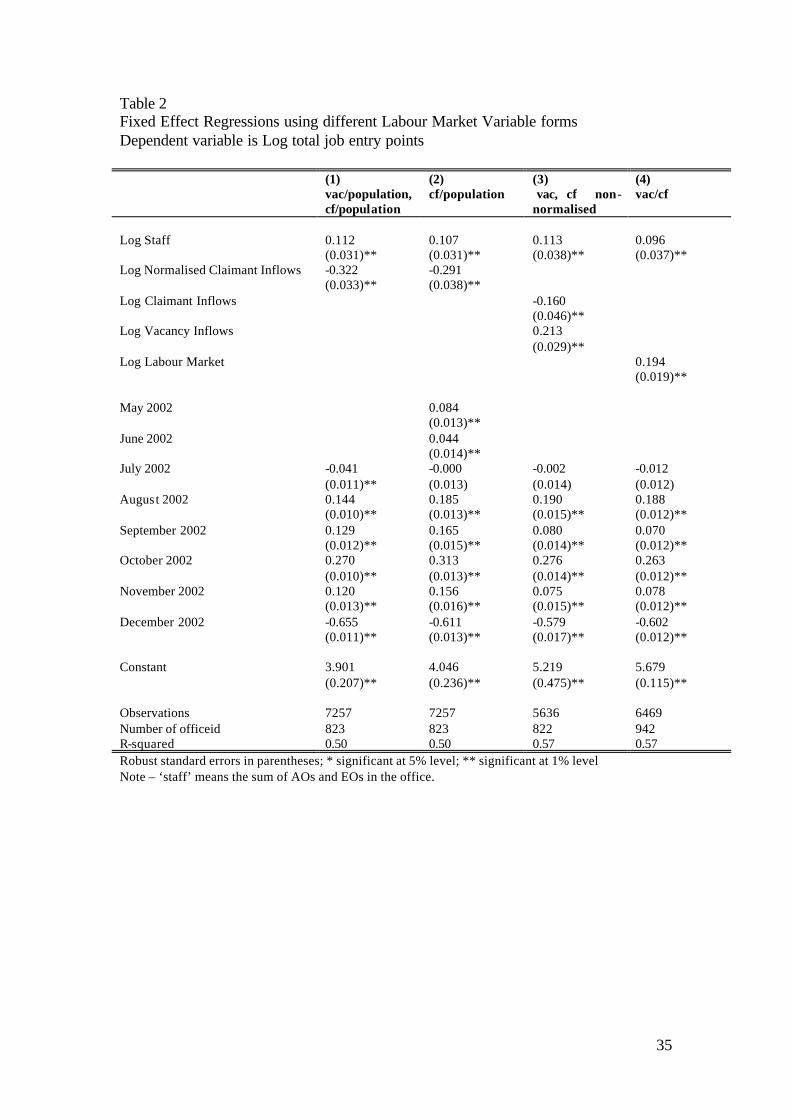
The dependent variable for tables 1-4 is the log total job entry points. As economic
theory suggests no obvious way of modelling the labour market conditions and the
relationship between job entry points and staff, we allow the data to influence our
results. Firstly table 1 and 2 look at various ways of modelling labour market
conditions. Our two labour market variables are claimant inflows and vacancy
inflows. The claimant inflow data is available for the whole evaluation period and
measures both the “raw material” of Jobcentres (so might be expected to positively
influence job entries) but are also a proxy for the state of the local labour market (and
hence would have a negative impact). The vacancy inflow data is available only
from June 2002, hence two months of evaluation period is lost from the start of the
scheme, however as noted above these months were before the workers were fully
announced to the staff. Vacancy inflows represent a partial measure of jobs available

17
to secure a job entry and will therefore have a positive effect. If we want to
normalise the flows to principally capture time series variation, we can use local
(TTWA) population, but this data is only available for England and Wales. So the
columns are not directly comparable as they are estimated on slightly different
datasets.
We find significant effects of the local labour market on job entries. In all cases,
vacancy inflows take the expected positive sign. The sign on claimant inflows varies
between specifications, but in the fixed effect regressions is always negative –
reflecting a worsening labour market. We show below that the office average effect
of claimant inflows is positive, which is intuitive as the long run average is a measure
of the amount of inflow JCP staff have to work with. The OLS regressions combine
both effects and so are positive in some columns in table 1. In column 4 we adopt a
specification that takes the log ratio of vacancy inflows to claimant inflows. This
normalises the variables without restricting the sample to England and Wales, has
support from the literature on matching functions, is accepted by our data and is the
specification adopted for the analysis. Our results show that a worsening labour
market makes it harder to secure job entries. This in turn makes it harder for staff to
achieve their targets and earn bonuses. The size and significance of the effect shows
the risk factor that staff bear is non-trivial.
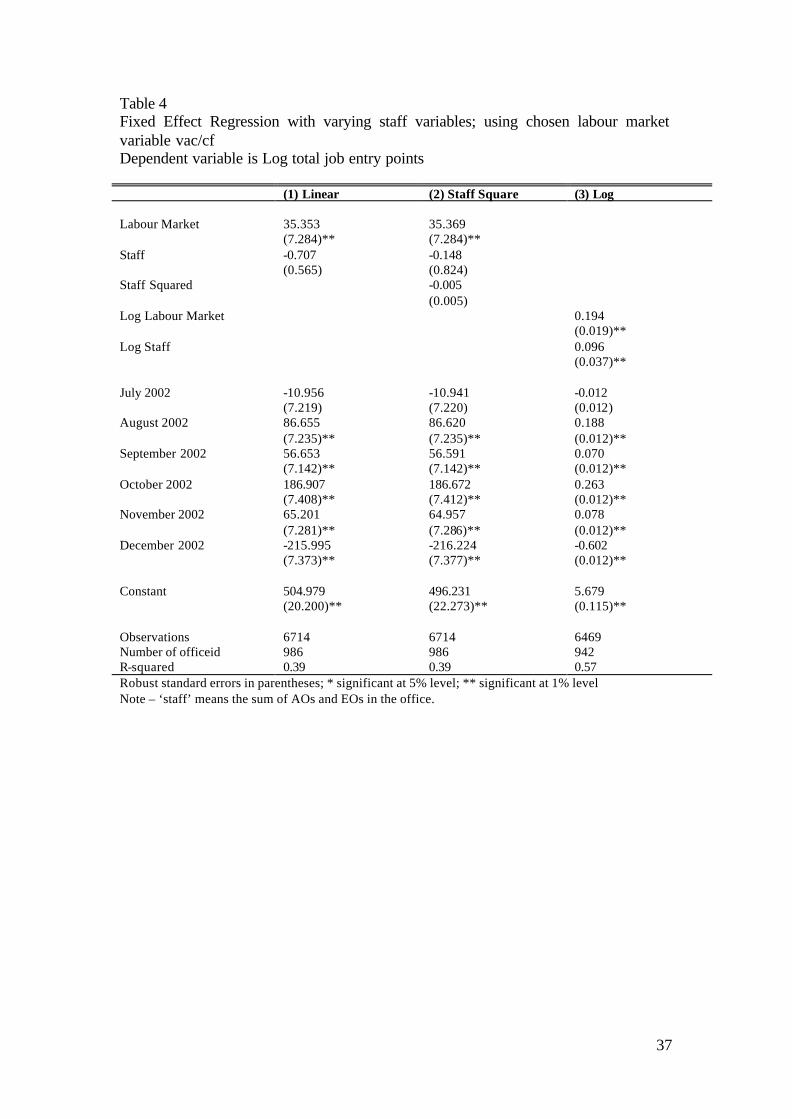
Turning to the staff data in table 3 and 4, as noted above, we take as our staff measure
the sum of the number of EOs and AOs in the office, staff- in-post and casuals. This is
highly correlated with any other sensible measure of staff, so we are confident that it
captures the true labour power available to office managers. For functional form, we
tried a simple linear model, a quadratic model and a log linear model.
Almost all of the variation in staff is across offices and very little over time within an
office. Therefore we expect the coefficients to be very different between the OLS and
the fixed effect estimation, and the tables bear this out. We find a very strong effect
of staff in the OLS, but very little in the panel analysis because it is simply absorbed
by the fixed effect. The specification in column 3 of table 4 (or column 4 in table 2)
is adopted for our eva luation, hence the regressions explain around half of the overall
variation in job entries. It is worth noting that there are strong seasonal effects for
job entry outcomes.

18
We extract the estimated office effects, and subject these to analysis. Note that these
necessarily have mean zero, but we adjust them by adding back the grand mean to
ensure they have the same mean as the equivalent raw data.
7.1.2 Second stage
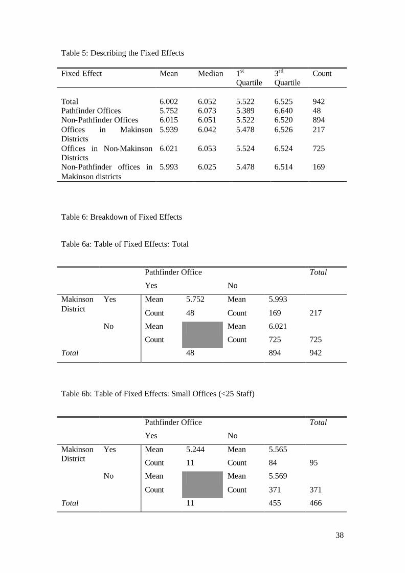
The office effects are average office job entry points after allowing for differences
across offices in staff, local labour market conditions and seasonal effects. Table 5
shows the mean and dispersion of these effects and figure 1 gives the full distribution.
The figure shows some large outliers at the left tail of the distribution, but otherwise
the pattern is reasonably normal. The table also shows some preliminary
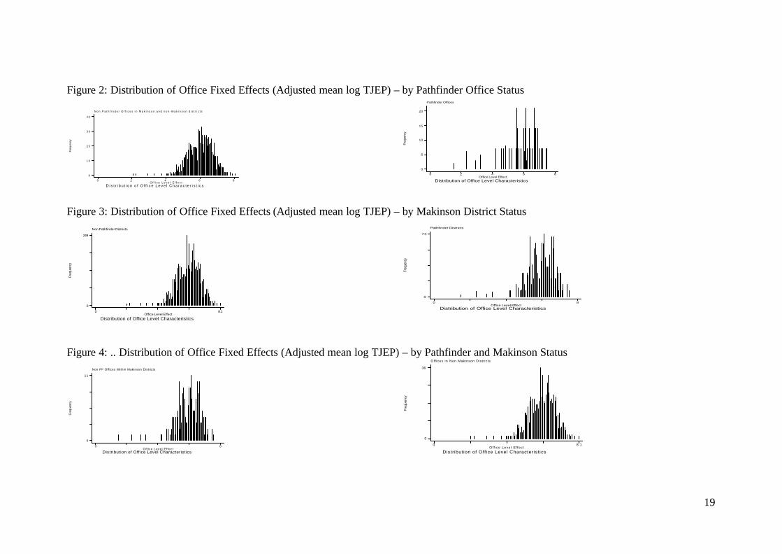
unconditional comparisons across different office and district types. Figures 2 to 4
present the whole distributions for these comparisons. Comparing offices in non-
Makinson districts with non-Pathfinder offices in Makinson districts is close to a like-
with- like comparison, and we see that the offices effects are fairly similar in the two
types of district, with the former being slightly higher. Pathfinder offices are clearly
associated with lower mean job entry figures. However the median and 3rd quartile of
Pathfinder offices achieve the highest job entries, evidence that although on average
the Pathfinder offices underachieve, those that perform well, outperform all other
offices.
Figure 1: Distribution of Office Fixed Effects (Adjusted mean log TJEP)
Fre
quen
cy
Distribution of Office level CharacteristicsOffice Level Effect
0 2 4 6 8
0
100
200
300
400
19
Figure 2: Distribution of Office Fixed Effects (Adjusted mean log TJEP) – by Pathfinder Office Status
N o n P a t h f i n d e r O f f i c e s i n M a k i n s o n a n d n o n - M a k i n s o n d i s t r i c t s
Freq
uenc
y
D i s t r i b u t i o n o f O f f i c e L e v e l C h a r a c t e r i s t i c sO f f i c e L e v e l E f f e c t
0 2 4 6 8
0
1 0
2 0
3 0
4 0
Figure 3: Distribution of Office Fixed Effects (Adjusted mean log TJEP) – by Makinson District Status Figure 4: .. Distribution of Office Fixed Effects (Adjusted mean log TJEP) – by Pathfinder and Makinson Status
Non PF Offices Within Makinson Districts
Freq
uenc
y
Distribution of Office Level CharacteristicsOffice Level Effect
0 8
0
11
Offices in Non Makinson Districts
Freq
uenc
y
Distribution of Office Level Characterist icsOff ice Level Ef fect
0 8.1
0
36
Pathfinder Offices
Freq
uenc
y
Distribution of Office Level CharacteristicsOffice Level Effect
0 2 4 6 8
0
5
10
15
20
Non Pathfinder Districts
Freq
uenc
y
Distribution of Office Level CharacteristicsOffice Level Effect
0 8.1
0
249
Pathfinder Districts
Freq
uenc
y
Distribution of Office Level CharacteristicsOffice Level Effect
0 8
0
73

20
Table 6 takes things a little further. Splitting the sample by office size and labour
market conditions we present data means again for a comparison of Pathfinder Office
and Makinson district status. We see that for small offices non-Pathfinder Makinson
offices perform similarly to non-Makinson offices while for larger offices, the non-
Makinson offices do better. There appears to be little difference by labour market
conditions. However, these comparisons do not allow for other factors so we turn to
regression analysis of these office averages to unravel the effect of different factors.
Before that, note the differences between the characteristics of offices in Makinson
and non-Makinson districts. Table 7 shows that offices in Makinson districts are
slightly bigger, less likely to be a District (“HQ”) office, have marginally worse
labour market conditions and are slightly more numerous per district.
Our main regression results are presented in tables 8 and 9. We start with basic
explanatory factors in column 1 of table 8. Big offices (defined in terms of staff)
produce more job entries; offices in labour markets with a lot of claimant inflows on
average produce more job entries (note that the labour market variable is vacancy
inflows/claimant inflows so a negative sign on the variable means a positive
relationship with job entries). These are both as expected. Offices having the status
of a District Office yield more job entries holding all else constant. A Pathfinder
office produces significantly fewer job entries than an otherwise equivalent office4.
The key variables we are interested in are the Makinson variables. Column 2 shows
that being in an incentivised district has an insignificant effect on job entries.
However, after allowing for heterogeneity of response by including an interaction of
Makinson status and office size (column 3), we find a significant Makinson effect.
Makinson has a positive effect that declines with office size. This effect fits our
predictions from the economic analysis presented above. Our interpretation is that
bigger offices face a greater free-rider problem and so the incentive payment is less
effective in eliciting higher effort. In column 4 we add a variable that measures the
number of offices in the district5, and allow its effect to differ in Makinson and non-
Makinson districts. It has no effect in the latter and a negative effect in the former.
This also has an interesting interpretation. It suggests that there is little interaction
4 This is presumably because staff in these offices are performing benefits-related activities as well as job entry tasks; it may also reflect the transitional disruption to the new status. 5 These are offices with positive job entries – not all JCP offices.

21
between offices in non-incentivised districts, but that it is attempted in incentivised
districts. The interaction is however far less effective in districts with many offices.
We examine whether the number of high grade staff in the office has any independent
effect but it appears not to. Finally using regional data from LFS, column 6 indicates
an adverse job entry effect from a private-public wage premium. The intuition is that
private sector wages in affluent areas are higher than in less affluent areas. For public
sector wages, the same is true but the difference will be smaller. Therefore it is likely
that in the affluent areas, high ability workers will be seduced by higher wages into
the private sector and a high private-public wage premium represents lower skilled
staff in public sector jobs. Deleting insignificant variables, we end up with the
preferred specification in column 7. This regression explains about half of the
variation between offices, and shows significant and heterogeneous effects from the
incentive scheme.
Inclusion of vacancy inflow as our choice of labour market variable could lead the
labour market variable to be endogenous. To ensure this is not the case we conduct
the above regressions on the fixed effect using just claimant inflow. The results,
detailed in Appendix 2 show no major change, either in the magnitude or significance
of the variables upon the office fixed effect.
7.1.3 Size of Office
The different effects of the scheme by size are interesting and important to the design
of the scheme. We therefore pursue them in a little more detail. Column 1 of table 9
breaks the effect up into different office size bands. We find that the effect of the
scheme does not decline monotonically with size, but the impact is roughly constant
until about 60 members of staff (this is AOs + EOs). In columns 3 to 4 we aim to
identify the cut-off point at which the costs from free riding exceed benefits from a
team-based incentive scheme. We tried cut-off points of 40 and 50 members of staff,
but the data prefer a cut-off of 60 staff. We present our final preferred specification in
column 6. This implies that the incentive scheme has an effect in offices up to size
60, and no effect thereafter. The Makinson effect declines with the number of offices
in a district. These results are reinforced by figure 5, which plots the Makinson effect
for various numbers of staff per office against the number of offices per district. It is
clear not only that the Makinson effect is decreasing in the number of offices per

22
district, but that this negative effect has far greater magnitude for large offices. To
get some feel for the importance of this, note that of the offices in the final regression,
847 out of the 942 are below 60, and 70% of staff (as measured by AO+EO measure)
are in such offices; 183 out of 217 Makinson offices (59% of staff) are below this cut-
off.
Figure 5
Sta
ff
Makinson Effect for Various Number of Staff per OfficeNumber of Offices per District
12 Staff 25 Staff 40 Staff 60 Staff
5 10 15 20 25
-.4
-.2
0
.2
.4
7.1.4 Size of Team
Across teams, or districts, the number of offices and staff varies substantively and it is
therefore interesting to evaluate the Makinson effect for various team sizes. The
number of offices within Makinson districts varies between 6 to 25, so we include an
interaction of Makinson status and the number of offices, divided into groups
accordingly. Column 1 of table 10 reports that relative to small districts (6-10
offices) large offices have lower job entries, although the results are not statistically
significant. The cut-off point is approximately 21 offices. Figure 6 shows that
although the Makinson effect is positive for districts with 11 or 18 offices per district,
it is always negative for districts with 21 offices. Similarly, the number of staff per
team affects the performance against the Job Entry target. The results in column 2
shows that, relative to small districts (defines as less than 364 staff members) large
districts have negative job entry points and in column 3 we see that any district

23
smaller than 771 staff will have greater output, relative to the larger offices.
Therefore for small teams, the incentive mechanism encouraging an increase in output
has stronger effects than the free rider problem. However as the team increases in
size this is no longer the case and the incentive scheme will not succeed in raising
output.
Figure 6
Offi
ces
Makinson Effect for Various Number of Offices per DistrictStaff
11 Offices 18 Offices 21 Offices
0 50 100
-.1
0
.1
.2
We can use these estimates to calculate the expected gain from the incentive scheme.
We compute the percentage gain for each district (for offices with less than 60) as:
100*((exp(0.308 – 0.014*#)-1)), where # represents the number of offices in that
district, and the coefficients 0.308 and 0.014 (this is 0.019 for Makinson districts
minus 0.005 for non-Makinson districts) are taken from column 3 of table 9. This
produces a conservative estimate and will if anything understate the effect, compared
to column 6. The results of this are in table 11. Districts with few offices show a
substantial gain. We expect that the districts with 15 or fewer offices per district to
achieve their stretch targets; the others may struggle to do so, because of having more
large offices, and many offices per district.

24
It needs to be re-emphasised that these estimates are only unbiased if the original
assignment of Makinson status to districts was random. To the extent that that is not
true, we may simply be picking up the effect of another characteristic that raises job
entry performance and is correlated with the assignment process.
7.1.5 Performance relative to the targets
We can analyse how the targets set during the year relate to job entry patterns, but
only for the Yorkshire and Humberside region where we have data on targets at
monthly level. Calderdale and Kirklees is the only Makinson district within
Yorkshire and Humberside and we analyse how performance in this district compares
to performance of the other nine districts in the region. In particular we analyse the
difference between actual performance and the target set.
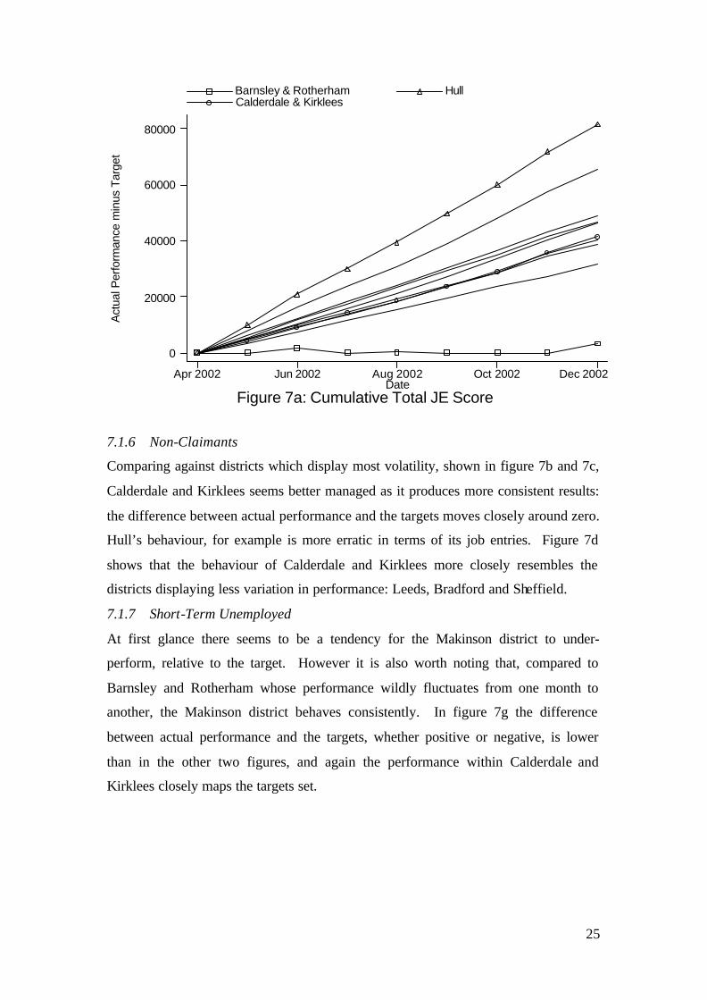
Figure 7a cumulates the difference between actual performance and targets over time,
from April 2002 to December 2002. Whilst Hull consistently performs at the highest
level and Barnsley and Rotherham the lowest relative to the targets, the performance
of the Makinson district is average.
We then focus on the Calderdale and Kirklees district, selecting the three job entry
client groups which this district was concentrating on and compare the change in
behaviour over time with the other districts. The purpose of this analysis is to gauge
whether there is any difference in the behaviour of the Makinson district over time,
with regard to its ability to hit the Job Entry target compared to the non- Makinson
districts. The highest number of job entries were achieved for the Non Claimant,
Short Term Unemployed and Employed categories. For clarity, the districts are
divided into groups which perform similarly and then compared to the Makinson
district.
25
Act
ual P
erfo
rman
ce m
inus
Tar
get
Figure 7a: Cumulative Total JE ScoreDate
Barnsley & Rotherham Hull Calderdale & Kirklees
Apr 2002 Jun 2002 Aug 2002 Oct 2002 Dec 2002
0
20000
40000
60000
80000
7.1.6 Non-Claimants
Comparing against districts which display most volatility, shown in figure 7b and 7c,
Calderdale and Kirklees seems better managed as it produces more consistent results:
the difference between actual performance and the targets moves closely around zero.
Hull’s behaviour, for example is more erratic in terms of its job entries. Figure 7d
shows that the behaviour of Calderdale and Kirklees more closely resembles the
districts displaying less variation in performance: Leeds, Bradford and Sheffield.
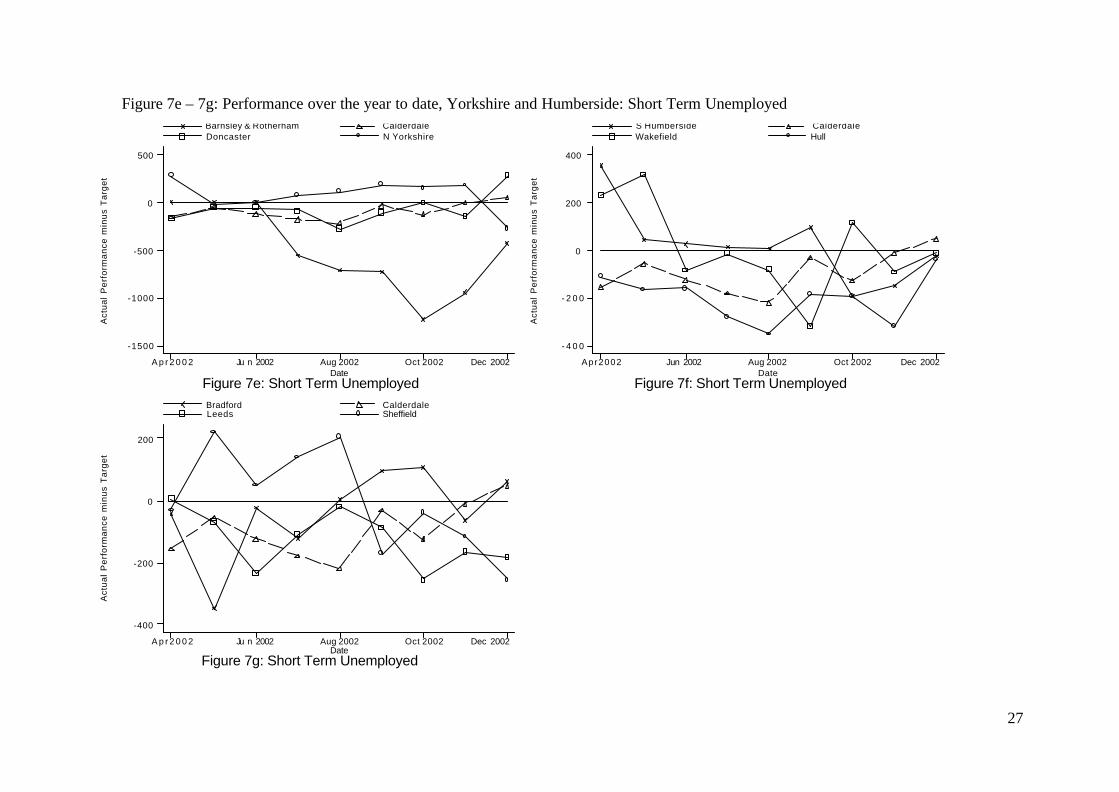
7.1.7 Short-Term Unemployed
At first glance there seems to be a tendency for the Makinson district to under-
perform, relative to the target. However it is also worth noting that, compared to
Barnsley and Rotherham whose performance wildly fluctuates from one month to
another, the Makinson district behaves consistently. In figure 7g the difference
between actual performance and the targets, whether positive or negative, is lower
than in the other two figures, and again the performance within Calderdale and
Kirklees closely maps the targets set.

26
Act
ua
l P
erf
orm
an
ce m
inu
s T
arg
et
Figure 7b: Non ClaimantsDate
S Humberside Calderdale Wakefield Hull
A p r 2 0 0 2 Jun 2002 Aug 2002 Oct 2002 Dec 2002
-200
0
200
400
600
Act
ua
l P
erf
orm
an
ce m
inu
s T
arg
et
Figure 7c: Non ClaimantsDate
Barnsley & Rotherham Calderdale Doncaster N Yorkshire
A p r 2 0 0 2 Jun 2002 Aug 2002 Oct 2002 Dec 2002
- 5 0 0
0
500
Act
ual
Per
form
ance
min
us T
arge
t
Figure 7d: Non ClaimantsDate
Bradford Calderdale Leeds Sheffield
A p r 2 0 0 2 Jun 2002 Aug 2002 Oct 2002 Dec 2002
-100
0
100
200
Figure 7b – 7d: Performance over the year to date, Yorkshire and Humberside: Non Claimants
27
Act
ua
l P
erf
orm
an
ce m
inu
s T
arg
et
Figure 7e: Short Term UnemployedDate
Barnsley & Rotherham Calderdale Doncaster N Yorkshire
A p r 2 0 0 2 Ju n 2002 Aug 2002 Oct 2002 Dec 2002
-1500
-1000
-500
0
500
Act
ua
l P
erf
orm
an
ce m
inu
s T
arg
et
Figure 7f: Short Term UnemployedDate
S Humberside Calderdale Wakefield Hull
Apr 2002 Jun 2002 Aug 2002 Oct 2002 Dec 2002
- 4 0 0
- 2 0 0
0
200
400
Act
ua
l P
erf
orm
an
ce m
inu
s T
arg
et
Figure 7g: Short Term UnemployedDate
Bradford Calderdale Leeds Sheffield
A p r 2 0 0 2 Ju n 2002 Aug 2002 Oct 2002 Dec 2002
-400
-200
0
200
Figure 7e – 7g: Performance over the year to date, Yorkshire and Humberside: Short Term Unemployed
28
Act
ua
l Pe
rfo
rma
nce
min
us
Ta
rge
t
Figure 7h: EmployedDate
S Humbers ide Ca lderda le Wakef ield Hull
A p r 2 0 0 2 Ju n 2002 Aug 2002 Oc t 2002 Dec 2002
0
200
400
Act
ua
l Pe
rfo
rma
nce
min
us
Ta
rge
t
Figure 7i: EmployedDate
Barns ley & Rotherham C a l d e r d a l e D o n c a s t e r N Yorkshire
A p r 2 0 0 2 Jun 2002 Aug 2002 Oct 2002 Dec 2002
- 1 0 0
0
100
200
Act
ua
l Pe
rfo
rma
nce
min
us
Ta
rge
t
Figure 7j: EmployedDate
Bradford Ca lderda le L e e d s Sheffield
A p r 2 0 0 2 Ju n 2002 Aug 2002 Oc t 2002 Dec 2002
- 5 0
0
5 0
100
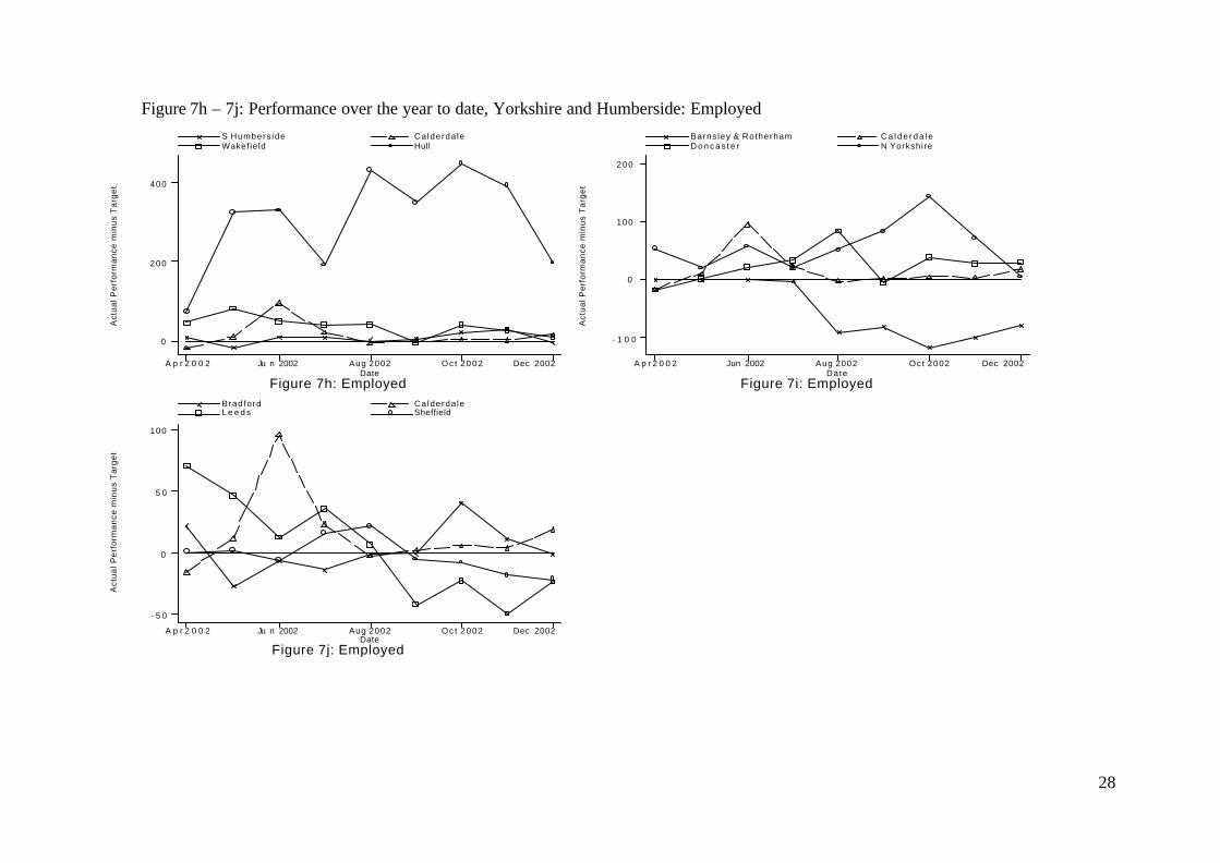
Figure 7h – 7j: Performance over the year to date, Yorkshire and Humberside: Employed

29
Figure 7b – 7j: Performance over the year to date, Yorkshire and Humberside 7.1.8 Employed
The achievement of Employed job entries relative to the target is close to zero for all
months in the Makinson district; more so than in other districts.
Comparing actual performance against targets, the district participating in the
incentive scheme exhibits less volatile performance: actual performance remains close
to the targets. This is not surprising giving the threshold nature of the scheme, as
performance above the level of the target is not rewarded.
7.2 Quality
The Customer Service target measures how well Jobcentres respond to the needs of
clients and employers using the Jobcentre services and is the first proxy for quality.
The second measure of quality is the Business Delivery target, which judges
performance against five Jobcentre Plus processes, incorporating aspects such as
accuracy and skill screening. We examine whether workers of the Jobcentres focus
upon achieving the job entries – quantity - at a cost to quality.
7.2.1 Customer Service
7.2.1.1 First Stage
We assume the functional form for the model which most represented the data in the
job entry analysis; a log linear model. Columns 1 and 3 of table 12 report the
coefficients from the OLS regression and columns 2 and 4 the Fixed Effect results.
We analyse the effect of both district log staff and district log job entries per member
of staff upon the quality measure. District staff have a negative effect upon the
Customer Service outcome, but columns 2 and 4 show that this is absorbed by the
district effect. There is evidence that as staff accumulate job entry points, there is a
decline in the Customer Service outcome, although the results are not significant. A
strong labour market (claimant inflows / vacancy inflows) tends to improve the
Customer Service outcome and again there are noted seasonal effects.

30
7.2.1.2 Second Stage
In table 13 we examine the relationship between variables which are likely to drive
working behaviour and the district Customer Service fixed effect. Paradoxically, staff
negatively impacts upon the Customer Service outcome. One reason for this could be
a lack of clarity of responsibility within the districts. The proportion of Pathfinder
offices within Makinson districts, Makinson status and Makinson status interacted
with staff do not statistically impact upon the Customer Service outcome. We know
from above that there is the size of the office is important in determining the effort
exerted towards achieving the job entry target. Unfortunately the Customer Service
target is measured at a district level, thus it is impossible to see whether the outcome
differs with office characteristics. However we can control for the number of offices
within the district, to examine whether small districts outperform larger districts. It
appears not to be the case as the variable is statistically insignificant, even when
interacted with the Makinson status.
7.2.2 Business Delivery
7.2.2.1 First Stage
The first stage regressions on log Business Delivery outcome, reported in table 14
also show a negative effect from staff which disappears once the district fixed effects
are controlled for. Across time and districts, job entry points per staff member
improve the outcome, but looking only across time there is an adverse (insignificant)
effect. The log labour market variable does not statistically influence the Business
Delivery outcome.
7.2.2.2 Second Stage
Table 15 reports the regression results on the district Business Delivery outcome.
Identified is a negative impact from staff upon the district Business Delivery score,
but similarly to the Customer Service outcome no other district level variables are
significant. All districts, whether participating in the incentive scheme or not do not
influence the outcome of the Business Delivery target.
The quality analysis generated results to suggest that the team defined by the district
does not entice workers to exert effort towards achieving the Customer Service or the
Business Delivery outcome. There are several interpretations for why such results

31
were generated. Firstly, the sample size is restricted to the 90 districts, with so few
degrees of freedom it is difficult to appropriately define the production function.
Secondly there may be free rider behaviour within the teams. The quality outcomes
are measured at an aggregated level and, as noted above the impact of individual
effort (whether the individual is the employee or the office) is hard to verify. In
contrast there was strong evidence of differential effort contribution towards the job
entry target, measured at office level. In particular, as already mentioned, in small
offices and districts, performance on job entries tends to be relatively high. Therefore,
the fact that the two quality outcomes do not vary with the number of offices per
district may suggest that workers do not try to improve performance on these targets
and their motivation is not so strong as for the job entry target – shirking is not easily
verifiable. Thirdly, multi-tasking issues traditionally emerge when measuring quantity
and quality, as quality elements are intrinsically measured with greater noise. This is
certainly true for the Jobcentre Plus quality measures. The Customer Service outcome
is measured by a mystery shopper approach and the five elements of the Business
Delivery target are recorded at different time periods, making it difficult for the
workers to understand how to improve their behaviour in such a way that would raise
the score achieved by the district. Given that all targets carry the same bonus, their
rational response would be to focus on tasks for which their effort is easily
transferable into outcomes: i.e. the quantity target.
In summary, we have analysed the effect of the Makinson scheme both on quantity
and on quality. We found strong results for the quantity analysis: the Makinson
scheme has had a significantly positive effect on job entries. This effect is smaller in
larger offices, and is smaller in districts with many offices. There was some evidence
of districts responding to the threshold nature of the scheme: exerting enough effort to
ensure that the target was hit, but not higher effort. The quality analysis was less
conclusive. However this is not entirely surprising, as the measures for quality are
collected at an aggregated level and may not be accurate in measuring the actions of
employees.
8 Future analysis
As noted above, this analysis of the team-based incentive scheme is preliminary and
we intend to advance the evaluation in a number of ways.

32
1. The time period of observation will be extended to incorporate information for full
four quarters in which the pilot scheme was run. Beyond that, we will collect and
use data from subsequent years to undertake a difference-in-difference analysis.
2. We will exploit the point system used to measure the job entry target, asking
whether the employees of Jobcentre Plus give precedence to clients deemed high
priority over other clients, in order to achieve more points towards the target.
There is a difficulty, as the workers will only behave in such a manner if the
reward for placing a high priority client (the points achieved) exceeds the cost of
doing so (the difficulty of placing the client into employment). The method by
which we do tackle the issue is to estimate the difficulty of placing lone parents
into employment6, using data on the number of lone parents actively seeking
employment at every Jobcentre office. If the Jobcentre staff do allocate jobs in
accordance with the design of the incentive scheme, we would expect to have
higher placements of lone parents, relative to other clients in areas with many lone
parents actively seeking employment.
3. We will use the estimated labour market impact to calibrate the labour market risk
facing JCP agents. Theory says that this should impact on the design of scheme.
Put differently, since we know it has not, there ought to be differential reaction to
the scheme in different labour market conditions. We will investigate this as a test
of the theory.
4. We will use the data to evaluate models of team incentives, the multi-tasking
aspects, and the potential role of public sector motivation.
5. It will be possible to calculate the number of job entries created through the
incentive scheme. Thus we can measure the output gained from the pilot scheme.
Then, once we know the end of year bonus payments we will conduct welfare
analysis, comparing the cost incurred from the incentive scheme to the cost
savings, in terms of reduced welfare payments.
9 Conclusion
Although there exists a wealth of economic theory on the implementation of financial
incentives in public services, our evaluation of the Jobcentre Plus incentive scheme is
to date the first empirical study in the UK. The complex nature of the scheme in

33
Jobcentre Plus has allowed us to explore the impact across many dimensions. Our
findings are that incentive schemes are more successful in small teams. We interpret
this as evidence that the free rider problem is mitigated in small teams by positive
attributes of team work, such as team morale and peer monitoring, however these
mechanisms weaken as teams grow in size. We observed strong, positive effects from
the incentive scheme upon quantity produced, but no real impact upon quality. This
may confirm theoretical predictions of multi- tasking – whereby workers focus their
effort upon targets measured with greater accuracy (i.e. quantity) and for which the
outcome of their actions is more easily verifiable. On the other hand, the finding may
reflect the small sample size available for quality analysis. Jobcentre Plus employees
seem to have responded to the threshold nature of the incentive scheme, exhibiting
gaming behaviour by aiming to exert effort enough to hit the target set, but not to
exceed the target. There are many more issues relating to the Jobcentre Plus incentive
scheme that we wish to investigate. However from the current analysis, evidence
suggests that the public sector employees did respond to the incentive scheme and
therefore with the appropriate design there is potential for improving the efficiency of
the public sector through the use of financial incentives.
6 Placement of Lone Parents into employment is rewarded with the maximum of 12 points

34
Table 1
OLS Regressions using different Labour Market Variable forms Dependent variable is Log total job entry points (1)
vac/population, cf/population
(2) cf/population
(3) vac, cf non-normalised
(4) vac/cf
Log Staff 0.660 0.647 0.680 0.698 (0.010)** (0.009)** (0.011)** (0.029)** Log Normalised Claimant Inflows 0.188 0.247 (0.029)** (0.026)** Log Normalised Vacancy Inflows 0.355 (0.029)** Log Claimant Inflows -0.093 (0.023)** Log Vacancy Inflows 0.104 (0.025)** Log Labour Market 0.082 (0.037)* May 2002 0.109 (0.029)** June 2002 -0.025 (0.029) July 2002 0.041 -0.040 -0.015 -0.025 (0.029) (0.029) (0.030) (0.015) August 2002 0.235 0.147 0.169 0.171 (0.029)** (0.029)** (0.030)** (0.012)** September 2002 0.048 0.064 0.108 0.095 (0.029) (0.030)* (0.030)** (0.015)** October 2002 0.297 0.289 0.274 0.270 (0.029)** (0.029)** (0.030)** (0.017)** November 2002 -0.000 0.005 0.057 0.060 (0.029) (0.030) (0.030) (0.016)** December 2002 -0.498 -0.608 -0.607 -0.621 (0.030)** (0.029)** (0.030)** (0.018)** Constant 6.832 5.365 3.785 3.839 (0.207)** (0.155)** (0.049)** (0.092)** Observations 5636 7257 5636 6469 R-squared 0.55 0.52 0.53 0.55 Robust standard errors in parentheses; * significant at 5% level; ** significant at 1% level Note – ‘staff’ means the sum of AOs and EOs in the office.
35
Table 2 Fixed Effect Regressions using different Labour Market Variable forms Dependent variable is Log total job entry points (1)
vac/population, cf/population
(2) cf/population
(3) vac, cf non-normalised
(4) vac/cf
Log Staff 0.112 0.107 0.113 0.096 (0.031)** (0.031)** (0.038)** (0.037)** Log Normalised Claimant Inflows -0.322 -0.291 (0.033)** (0.038)** Log Claimant Inflows -0.160 (0.046)** Log Vacancy Inflows 0.213 (0.029)** Log Labour Market 0.194 (0.019)** May 2002 0.084 (0.013)** June 2002 0.044 (0.014)** July 2002 -0.041 -0.000 -0.002 -0.012 (0.011)** (0.013) (0.014) (0.012) August 2002 0.144 0.185 0.190 0.188 (0.010)** (0.013)** (0.015)** (0.012)** September 2002 0.129 0.165 0.080 0.070 (0.012)** (0.015)** (0.014)** (0.012)** October 2002 0.270 0.313 0.276 0.263 (0.010)** (0.013)** (0.014)** (0.012)** November 2002 0.120 0.156 0.075 0.078 (0.013)** (0.016)** (0.015)** (0.012)** December 2002 -0.655 -0.611 -0.579 -0.602 (0.011)** (0.013)** (0.017)** (0.012)** Constant 3.901 4.046 5.219 5.679 (0.207)** (0.236)** (0.475)** (0.115)** Observations 7257 7257 5636 6469 Number of officeid 823 823 822 942 R-squared 0.50 0.50 0.57 0.57 Robust standard errors in parentheses; * significant at 5% level; ** significant at 1% level Note – ‘staff’ means the sum of AOs and EOs in the office.

36
Table 3 OLS Regression with varying staff variables; using chosen labour market variable as vac/cf Dependent variable is Log total job entry points (1) Linear (2) Quadratic (3) Log Labour Market -6.228 13.696 (8.376) (7.951) Staff 9.090 14.957 (0.166)** (0.260)** Staff Squared -0.036 (0.001)** Log Labour Market 0.082 (0.020)** Log Staff 0.698 (0.009)** July 2002 -17.874 -14.785 -0.025 (16.828) (15.911) (0.027) August 2002 79.913 83.000 0.171 (16.837)** (15.920)** (0.027)** Septemb er 2002 62.106 61.288 0.095 (16.782)** (15.868)** (0.027)** October 2002 192.378 182.450 0.270 (17.139)** (16.209)** (0.027)** November 2002 59.198 52.946 0.060 (17.058)** (16.131)** (0.027)* December 2002 -225.720 -228.969 -0.621 (17.109)** (16.178)** (0.027)** Constant 270.588 131.987 3.839 (17.515)** (17.275)** (0.034)** Observations 6714 6714 6469 R-squared 0.36 0.43 0.55 Robust standard errors in parentheses; * significant at 5% level; ** significant at 1% level Note – ‘staff’ means the sum of AOs and EOs in the office.
37
Table 4 Fixed Effect Regression with varying staff variables; using chosen labour market variable vac/cf Dependent variable is Log total job entry points (1) Linear (2) Staff Square (3) Log Labour Market 35.353 35.369 (7.284)** (7.284)** Staff -0.707 -0.148 (0.565) (0.824) Staff Squared -0.005 (0.005) Log Labour Market 0.194 (0.019)** Log Staff 0.096 (0.037)** July 2002 -10.956 -10.941 -0.012 (7.219) (7.220) (0.012) August 2002 86.655 86.620 0.188 (7.235)** (7.235)** (0.012)** September 2002 56.653 56.591 0.070 (7.142)** (7.142)** (0.012)** October 2002 186.907 186.672 0.263 (7.408)** (7.412)** (0.012)** November 2002 65.201 64.957 0.078 (7.281)** (7.286)** (0.012)** December 2002 -215.995 -216.224 -0.602 (7.373)** (7.377)** (0.012)** Constant 504.979 496.231 5.679 (20.200)** (22.273)** (0.115)** Observations 6714 6714 6469 Number of officeid 986 986 942 R-squared 0.39 0.39 0.57 Robust standard errors in parentheses; * significant at 5% level; ** significant at 1% level Note – ‘staff’ means the sum of AOs and EOs in the office.
38
Table 5: Describing the Fixed Effects Fixed Effect Mean Median 1st
Quartile 3rd Quartile
Count
Total 6.002 6.052 5.522 6.525 942 Pathfinder Offices 5.752 6.073 5.389 6.640 48 Non-Pathfinder Offices 6.015 6.051 5.522 6.520 894 Offices in Makinson Districts
5.939 6.042 5.478 6.526 217
Offices in Non-Makinson Districts
6.021 6.053 5.524 6.524 725
Non-Pathfinder offices in Makinson districts
5.993 6.025 5.478 6.514 169
Table 6: Breakdown of Fixed Effects
Table 6a: Table of Fixed Effects: Total
Pathfinder Office Total
Yes No
Makinson District
Yes Mean
Count
5.752
48
Mean
Count
5.993
169
217
No Mean
Count
Mean
Count
6.021
725
725
Total 48 894 942
Table 6b: Table of Fixed Effects: Small Offices (<25 Staff)
Pathfinder Office Total
Yes No
Makinson District
Yes Mean
Count
5.244
11
Mean
Count
5.565
84
95
No Mean
Count
Mean
Count
5.569
371
371
Total 11 455 466

39
Table 6c: Table of Fixed Effects: Large Offices (>=25 Staff)
Pathfinder Office Total
Yes No
Makinson District
Yes Mean
Count
5.903
37
Mean
Count
6.415
85
122
No Mean
Count
Mean
Count
6.493
354
354
Total 37 439 476
Table 6d: Table of Fixed Effects: Good (above average) Labour Market Conditions
Pathfinder Office Total
Yes No
Makinson District
Yes Mean
Count
5.167
15
Mean
Count
5.763
71
86
No Mean
Count
Mean
Count
5.793
276
276
Total 15 347 362
Table 6e: Table of Fixed Effects: Poor (below average) Labour Market Conditions
Pathfinder Office Total
Yes No
Makinson District
Yes Mean
Count
6.018
33
Mean
Count
6.159
98
131
No Mean
Count
Mean
Count
6.161
449
449
Total 33 547 580
Note – ‘staff’ means the sum of AOs and EOs in the office.

40
Table 7: Office characteristics summary by Makinson District Status Pathfinder Office
(%) Staff (AO + EO)
Number of offices in District
District (HQ) Office (%)
Mean labour market conditions
Offices in Non- Mean 29.47 11.354 0.105 0.189 Makinson Districts Median 24 11 0 0.144 Sd 26.76 4.061 0.307 0.335 Q10 7 6 0 -0.142 Q90
57 17 1 0.612 Offices in Mean 0.221 36.111 14.475 0.065 0.182 Makinson Districts Median 0 27 16 0 0.176 Sd 0.416 32.727 5.156 0.246 0.26 Q10 0 8 7 0 -0.129 Q90 1 78 22 0 0.545 All offices Mean 0.051 31 12.073 0.096 0.187 Median 0 25 12 0 0.175 Sd 0.22 28.366 4.53 0.294 0.319 Q10 0 8 7 0 -0.129 Q90 0 61 17 0 0.57 Note – ‘staff’ means the sum of AOs and EOs in the office.

41
Table 8: Regressions on the Fixed Effects Dependent variable is Office Fixed Effect 1 2 3 4 5 6 7 Pathfinder Office -0.697 -0.682 -0.537 -0.582 -0.581 -0.576 -0.576 (0.085)** (0.093)** (0.105)** (0.106)** (0.106)** (0.106)** (0.105)** District Office 0.251 0.249 0.238 0.234 0.233 0.238 0.239 (0.064)** (0.065)** (0.064)** (0.064)** (0.064)** (0.064)** (0.064)** log Staff 0.557 0.557 0.586 0.583 0.583 0.589 0.593 (0.023)** (0.023)** (0.025)** (0.026)** (0.026)** (0.026)** (0.025)** Mean labour market conditions -0.135 -0.136 -0.131 -0.125 -0.125 -0.139 -0.139 (0.039)** (0.039)** (0.039)** (0.038)** (0.038)** (0.039)** (0.039)** Makinson District Status -0.019 0.099 0.432 0.429 0.408 0.467 (0.048) (0.063) (0.146)** (0.147)** (0.147)** (0.133)** Makinson Status*Staff -0.004 -0.005 -0.005 -0.005 -0.005 (0.001)** (0.001)** (0.001)** (0.001)** (0.001)** Number of Offices in District -0.004 -0.004 -0.004 (0.005) (0.005) (0.005) Makinson Status*Number of offices -0.02 -0.02 -0.019 -0.024 (0.009)* (0.009)* (0.009)** (0.008)** % High grade staff in office -0.239 -0.254 (0.559) (0.557) Private Public Wage Gap -0.018 -0.018 (0.008)* (0.008)* Constant 4.459 4.463 4.369 4.421 4.429 4.431 4.356 (0.097)** (0.098)** (0.103)** (0.126)** (0.127)** (0.127)** (0.102)** Observations 942 942 942 942 942 942 942 R-squared 0.46 0.45 0.46 0.47 0.47 0.47 0.47 Note – ‘staff’ means the sum of AOs and EOs in the office. Standard errors in parentheses; * significant at 5% level; ** significant at 1% level

42
Table 9: Regressions on the Fixed Effects – Alternative Size Variables Dependent variable is Office Fixed Effect 1 2 3 4 5 6 Makinson Office, staff <= 12 0.262 0.333 (0.160) (0.146)* Makinson Office, 12 < staff <= 25 0.285 0.351 (0.159) (0.147)* Makinson Office, 25 < staff <= 40 0.351 0.413 (0.150)* (0.138)** Makinson Office, 40 < staff <= 60 0.293 0.353 (0.161) (0.152)* Makinson Office, staff > 60 0.016 0.073 -0.285 -0.292 (0.168) (0.159) (0.120)* (0.120)* Makinson District Status 0.308 0.282 0.299 0.371 (0.137)* (0.137)* (0.140)* (0.124)** Makinson Office, staff > 50 -0.181 (0.115) Makinson Office, staff > 40 -0.124 (0.094) Number of Offices in District -0.006 -0.005 -0.006 -0.006 (0.005) (0.005) (0.005) (0.005) Makinson Status*Number of offices -0.018 -0.024 -0.019 -0.017 -0.018 -0.024 (0.009) (0.008)** (0.009)* (0.009) (0.009) (0.008)** Observations 942 942 942 942 942 942 R-squared 0.46 0.46 0.46 0.46 0.46 0.46 Note – also included in the regressions are intercept, Pathfinder Office status, District Office status, log staff, and mean labour market conditions; the coefficients not shown but available from the authors. Note – ‘staff’ means the sum of AOs and EOs in the office. Standard errors in parentheses; * significant at 5% level; ** significant at 1% level

43
Table 10: Alternative Team Sizes Dependent variable is Office Fixed Effect 1 2 3 Makinson District, 10 < offices <= 17 0.032 (0.144) Makinson District, 18 < offices <= 20 -0.249 (0.161) Makinson District, offices <= 21 -0.243 (0.147) Makinson District, 364 < staff 0.210 (0.079)** Makinson District, 365 < staff <= 550 -0.102 0.108 (0.081) (0.107) Makinson District, 551 < staff <= 770 -0.071 0.139 (0.081) (0.106) Makinson District, staff <= 771 -0.210 (0.079)** Observations 942 942 R-squared 0.46 0.46 Note – also included in the regressions are intercept, Pathfinder Office status, District Office status, log staff, and mean labour market
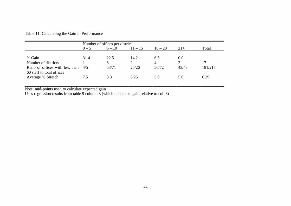
44
Table 11: Calculating the Gain in Performance Number of offices per district 0 – 5 6 – 10 11 – 15 16 – 20 21+ Total % Gain 31.4 22.5 14.2 6.5 0.0 Number of districts 1 8 2 4 2 17 Ratio of offices with less than 60 staff to total offices
4/5 53/71 25/26 56/72 43/43 181/217
Average % Stretch 7.5 8.3 6.25 5.0 5.0 6.29
Note: mid-points used to calculate expected gain Uses regression results from table 9 column 3 (which understate gain relative to col. 6)

45
Table 12: OLS and Fixed Effect Regressions Dependent Variable is Log Customer Service Outcome 1 2 3 4 District Log Staff -0.012 0.086 (0.005)* (0.057) District Log (Job Entries/Staff) -0.001 -0.001 (0.003) (0.003) District Log Labour Market 0.016 0.011 0.021 0.006 (0.009) (0.019) (0.009)* (0.020) September 2002 -0.022 -0.020 -0.022 -0.023 (0.005)** (0.003)** (0.005)** (0.003)** December 2002 0.000 0.000 0.000 0.000 (0.000) 0.000 (0.000) (0.000) Constant -0.180 -0.060 -0.165 -0.161 (0.007)** (0.069) (0.004)** (0.005)** Observations 180 180 174 174 Number of districtid 90 90 R-squared 0.17 0.37 0.14 0.39

46
Table 13: Regressions on the Fixed Effect Dependent Variable is District CST Fixed Effect 1 3 4 5 6 7 District log Staff -0.097 -0.096 -0.101 -0.102 -0.111 -0.112 (0.007)** (0.007)** (0.007)** (0.008)** (0.010)** (0.010)** District Mean labour market conditions 0.007 0.009 0.008 0.008 0.002 0.002 (0.008) (0.008) (0.008) (0.008) (0.008) (0.008) Makinson District Status 0.015 0.013 0.013 0.019 (0.008) (0.018) (0.018) (0.021) Makinson Status*Staff 0.005 0.001 0.013 (0.038) (0.038) (0.045) Number of Offices in District 0.002 0.002 (0.001) (0.001) Makinson Status*Number of offices -0.001 (0.002) % PF offices within the district -0.006 -0.008 -0.008 -0.008 -0.009 (0.005) (0.005) (0.005) (0.005) (0.005) Constant -0.291 -0.217 -0.209 -0.208 -0.220 -0.222 (0.011)** (0.058)** (0.058)** (0.058)** (0.058)** (0.058)** Observations 90 90 90 90 90 90 R-squared 0.74 0.74 0.75 0.75 0.76 0.76

47
Table 14: OLS and Fixed Effect Regressions Dependent Variable is Log Business Delivery Outcome 1 2 3 4 District Log Staff -0.013 0.020 (0.006)* (0.037) District Log (Job Entries/Staff) 0.008 -0.002 (0.003) (0.002) District Log Labour Market -0.008 -0.004 0.000 -0003 (0.012) (0.016 (0.011) (0.016) September 2002 0.010 0.006 0.006 0.007 (0.010) (0.005) (0.010) (0.005) October 2002 0.002 0.006 -0.003 0.007 (0.010) (0.005) (0.010) (0.006) November 2002 0.012 0.016 0.009 0.017 (0.010) (0.005)** (0.010) (0.005)** December 2002 0.000 0.000 0.000 0.000 (0.000) 0.000 (0.000) (0.000) Constant 4.488 4.525 4.500 4.500 (0.011)** (0.046)** (0.009)** (0.006)** Observations 287 287 285 285 Number of districtid 89 89 R-squared 0.03 0.09 0.04 0.09

48
Table 15: Regressions on the Fixed Effect Dependent Variable is District BDT Fixed Effect 1 2 3 4 5 6 District log Staff -0.034 -0.033 -0.040 -0.038 -0.044 -0.050 (0.012)** (0.012)** (0.013)** (0.015)* (0.017)* (0.017)** District Mean labour market conditions -0.016 -0.015 -0.018 -0.018 -0.022 -0.020 (0.015) (0.016) (0.016) (0.016) (0.016) (0.016) Makinson District Status 0.019 0.029 0.029 0.064 (0.014) (0.032) (0.032) (0.038) Makinson Status*Staff -0.023 -0.026 0.041 (0.069) (0.069) (0.080) Number of Offices in District 0.001 0.002 (0.001) (0.002) Makinson Status*Number of offices -0.005 (0.003) % PF offices within the district -0.004 -0.005 -0.005 -0.005 -0.006 (0.008) (0.009) (0.009) (0.009) (0.009) Constant 4.479 4.522 4.531 4.528 4.520 4.512 (0.021)** (0.104)** (0.103)** (0.105)** (0.105)** (0.104)** Observations 89 89 89 89 89 89 R-squared 0.08 0.08 0.10 0.10 0.11 0.14

49
References
S. Burgess, M.L. Ratto “The role of incentives in the public sector: issues and
evidence”, Oxford Review of Economic Policy, 2003, (forthcoming).
A. Dixit “Incentives and organisations in the public sector: an interpretative review”
Journal of Human Resources, vol 37(4), Fall 2002, 696-727.
B. Holmström “Moral hazard in teams”, Bell Journal of Economics, 13, 1982, 324-340.
B. Holmström, P. Milgrom. “Regulating trade among agents”, Journal of Institutional
and Theoretical Economics, vol. 146(1), 1990, 85-105. B. Holmström, P. Milgrom “Multi-task principal-agent analyses: Linear contracts, asset ownership and job design”, Journal of Law, Economics and Organisation, vol 7, 1991, 24-52. H. Itoh “Incentives to help in multi-agent situations”, Econometrica, vol 59, (3),1991,
611-636.
J. Makinson “Incentives for change. Rewarding performance in national government networks”, Public Service Productivity Panel, 2000.
G. MacDonald, L. M. Max “Adverse Specialization”, Journal of Political Economy, vol 109 (4), 2001, 864-899.
C. Prendergast “The provision of incentives in firms”, Journal of Economic
Literature, vol 37, 1999, 7-63.

50
Appendices
Appendix 1: Job Entry Priority Group Categories Priority Client Group 1 Job entry points score 12 Jobless Lone Parents including people on the New Deal for Lone Parents Those on the New Deal for Disabled People People with Disabilities in receipt of a specified primary benefit Other people in receipt of a specified primary benefit Priority Client Group 2 Job entry points score 8 People on the New Deal 50 plus People on the New Deal 25 plus Those on the New Deal for Young People Employment Zones Other People with Disabilities not included in Priority Client Group 1 Jobseeker’s Allowance (JSA) long term claimants Priority Client Group 3 Job entry points score 4 JSA short term claimants Priority Client Group 4 Job entry points score 2 Unemployed non claimants Priority Client Group 5 Job entry points score 1 Employed People

51
Appendix 2: Regressions on the Fixed Effects using Claimant Inflow as the Labour Market Variable Dependent variable is Office Fixed Effect 1 2 3 4 5 6 7 Pathfinder Office -0.719 -0.728 -0.589 -0.650 -0.649 -0.621 -0.618
(0.100)** (0.110)** (0.125)** (0.125)** (0.125)** (0.124)** (0.124)**
District Office 0.186 0.187 0.174 0.172 0.170 0.188 0.191
(0.076)* (0.077)* (0.077)* (0.076)* (0.076)* (0.076)* (0.076)*
log Staff 0.723 0.723 0.752 0.739 0.739 0.727 0.740
(0.028)** (0.028)** (0.030)** (0.031)** (0.031)** (0.030)** (0.030)**
Mean Claimant Inflow 0.034 0.034 0.034 0.034 0.034 0.048 0.048
(0.002)** (0.002)** (0.002)** (0.002)** (0.002)** (0.004)** (0.004)**
Makinson District Status 0.010 0.126 0.386 0.380 0.316 0.514
(0.057) (0.076) (0.179)* (0.179)* (0.178) (0.161)**
Makinson Status*Staff -0.004 -0.004 -0.004 -0.004 -0.004
(0.002)* (0.002)* (0.002)* (0.002)* (0.002)*
Number of Offices in District -0.014 -0.014 -0.015
(0.006)* (0.006)* (0.006)*
Makinson Status*Number of offices -0.012 -0.011 -0.008 -0.023
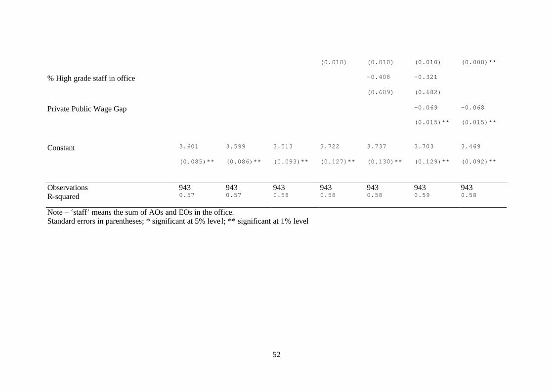
52
(0.010) (0.010) (0.010) (0.008)**
% High grade staff in office -0.408 -0.321
(0.689) (0.682)
Private Public Wage Gap -0.069 -0.068
(0.015)** (0.015)**
Constant 3.601 3.599 3.513 3.722 3.737 3.703 3.469
(0.085)** (0.086)** (0.093)** (0.127)** (0.130)** (0.129)** (0.092)**
Observations 943 943 943 943 943 943 943 R-squared 0.57 0.57 0.58 0.58 0.58 0.59 0.58
Note – ‘staff’ means the sum of AOs and EOs in the office. Standard errors in parentheses; * significant at 5% leve l; ** significant at 1% level